Embed Size (px)
Citation preview

Published as a conference paper at ICLR 2018
CAUSALGAN: LEARNING CAUSAL IMPLICIT GENER-ATIVE MODELS WITH ADVERSARIAL TRAINING
Murat Kocaoglu∗, Christopher Snyder∗, Alexandros G. Dimakis,Sriram Vishwanath
Department of Electrical and Computer EngineeringThe University of Texas at Austin
Austin, TX, [email protected],[email protected],
[email protected],[email protected]
ABSTRACT
We introduce causal implicit generative models (CiGMs): models that allow sam-pling from not only the true observational but also the true interventional distri-butions. We show that adversarial training can be used to learn a CiGM, if thegenerator architecture is structured based on a given causal graph. We consider theapplication of conditional and interventional sampling of face images with binaryfeature labels, such as mustache, young. We preserve the dependency structurebetween the labels with a given causal graph. We devise a two-stage procedurefor learning a CiGM over the labels and the image. First we train a CiGM overthe binary labels using a Wasserstein GAN where the generator neural networkis consistent with the causal graph between the labels. Later, we combine thiswith a conditional GAN to generate images conditioned on the binary labels. Wepropose two new conditional GAN architectures: CausalGAN and CausalBEGAN.We show that the optimal generator of the CausalGAN, given the labels, samplesfrom the image distributions conditioned on these labels. The conditional GANcombined with a trained CiGM for the labels is then a CiGM over the labels and thegenerated image. We show that the proposed architectures can be used to samplefrom observational and interventional image distributions, even for interventionswhich do not naturally occur in the dataset.
1 INTRODUCTION
An implicit generative model (Mohamed & Lakshminarayanan (2016)) is a mechanism that can sam-ple from a probability distribution without an explicit parameterization of the likelihood. Generativeadversarial networks (GANs) arguably provide one of the most successful ways to train implicitgenerative models. GANs are neural generative models that can be trained using backpropagationto sample from very high dimensional nonparametric distributions (Goodfellow et al. (2014)). Agenerator network models the sampling process through feedforward computation given a noisevector. The generator output is constrained and refined through feedback by a competitive adversarynetwork, called the discriminator, that attempts to distinguish between the generated and real samples.The objective of the generator is to maximize the loss of the discriminator (convince the discriminatorthat it outputs samples from the real data distribution). GANs have shown tremendous success ingenerating samples from distributions such as image and video (Vondrick et al. (2016)).
An extension of GANs is to enable sampling from the class conditional data distributions by feedingclass labels to the generator alongside the noise vectors. Various neural network architectures havebeen proposed for solving this problem (Mirza & Osindero (2014); Odena et al. (2016); Antipov et al.
∗Equal contribution
1

Published as a conference paper at ICLR 2018
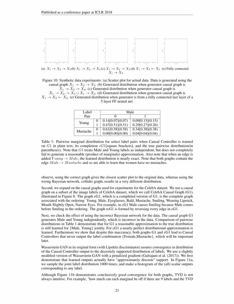
(a) Top: Intervened on Bald=1. Bottom: Condi-tioned on Bald = 1. Male→ Bald.
(b) Top: Intervened on Mustache=1. Bottom: Con-ditioned on Mustache = 1. Male→Mustache.
Figure 1: Observational and interventional samples from CausalBEGAN. Our architecture canbe used to sample not only from the joint distribution (conditioned on a label) but also from theinterventional distribution, e.g., under the intervention do(Mustache = 1). The two distributionsare clearly different since P(Male = 1|Mustache = 1) = 1 and P(Bald = 1|Male = 0) = 0 inthe data distribution P.
(2017)). However, these architectures do not capture the dependence between the labels. Therefore,they do not have a mechanism to sample images given a subset of the labels, since they cannot samplethe remaining labels. In this paper, we are interested in extending the previous work on conditionalimage generation by i) capturing the dependence between labels and ii) capturing the causal effectbetween labels. We can think of conditional image generation as a causal process: Labels determinethe image distribution. The generator is a non-deterministic mapping from labels to images. This isconsistent with the causal graph "Labels cause the Image", denoted by L→ I , where L is the randomvector for labels and I is the image random variable. Using a finer model, we can also include thecausal graph between the labels, if available.
As an example, consider the causal graph between Gender (G) and Mustache (M ) labels. The causalrelation is clearly Gender causes Mustache, denoted by the graph G→M . Conditioning on Gender= male, we expect to see males with or without mustaches, based on the fraction of males withmustaches in the population. When we condition on Mustache = 1, we expect to sample from malesonly since the population does not contain females with mustaches. In addition to sampling fromconditional distributions, causal models allow us to sample from various different distributions calledinterventional distributions. An intervention is an experiment that fixes the value of a variable ina causal graph. This affects the distributions of the descendants of the intervened variable in thegraph. But unlike conditioning, it does not affect the distribution of its ancestors. For the same causalgraph, intervening on Mustache = 1 would not change the distribution of Gender. Accordingly, thelabel combination (Gender = female, Mustache = 1) would appear as often as Gender = female afterthe intervention. Please see Figure 1 for some of our conditional and interventional samples, whichillustrate this concept on the Bald and Mustache variables.
In this work we propose causal implicit generative models (CiGM): mechanisms that can samplenot only from the correct joint probability distributions but also from the correct conditional andinterventional probability distributions. Our objective is not to learn the causal graph: we assumethat the true causal graph is given to us. We show that when the generator structure inherits its neuralconnections from the causal graph, GANs can be used to train causal implicit generative models. Weuse Wasserstein GAN (WGAN) (Arjovsky et al. (2017)) to train a CiGM for binary image labels, asthe first step of a two-step procedure for training a CiGM for the images and image labels. For thesecond step, we propose two novel conditional GANs called CausalGAN and CausalBEGAN. Weshow that the optimal generator of CausalGAN can sample from the true conditional distributions(see Theorem 1).
We show that combining CausalGAN with a CiGM on the labels yields a CiGM on the labels and theimage, which is formalized in Corollary 1 in Section 5. Our contributions are as follows:
• We observe that adversarial training can be used after structuring the generator architecturebased on the causal graph to train a CiGM. We empirically show that WGAN can be used tolearn a CiGM that outputs essentially discrete1 labels, creating a CiGM for binary labels.• We consider the problem of conditional and interventional sampling of images given a
causal graph over binary labels. We propose a two-stage procedure to train a CiGM over thebinary labels and the image. As part of this procedure, we propose a novel conditional GAN
1Each of the generated labels is sharply concentrated around 0 or 1 (Please see Figure 11a in the Appendix).
2

Published as a conference paper at ICLR 2018
architecture and loss function. We show that the global optimal generator provably samplesfrom the class conditional distributions.• We propose a natural but nontrivial extension of BEGAN to accept labels: using the same
motivations for margins as in BEGAN (Berthelot et al. (2017)), we arrive at a "marginof margins" term. We show empirically that this model, which we call CausalBEGAN,produces high quality images that capture the image labels.• We evaluate our CiGM training framework on the labeled CelebA data (Liu et al. (2015)).
We empirically show that CausalGAN and CausalBEGAN can produce label-consistentimages even for label combinations realized under interventions that never occur duringtraining, e.g., "woman with mustache"2.
2 RELATED WORK
Using a GAN conditioned on the image labels has been proposed before: In Mirza & Osindero(2014), authors propose conditional GAN (CGAN): They extend generative adversarial networksto the setting where there is extra information, such as labels. Image labels are given to both thegenerator and the discriminator. In Odena et al. (2016), authors propose ACGAN: Instead of receivingthe labels as input, the discriminator is now tasked with estimating the label. In Sricharan et al.(2017), the authors compare the performance of CGAN and ACGAN and propose an extension to thesemi-supervised setting. In Chen et al. (2016), authors propose a new architecture called InfoGAN,which attempts to maximize a variational lower bound of mutual information between the inputsgiven to the generator and the image. To the best of our knowledge, the existing conditional GANsdo not allow sampling from label combinations that do not appear in the dataset (Sricharan (2017)).
BiGAN (Donahue et al. (2017b)) and ALI (Dumoulin et al. (2017)) extend the standard GANframework by also learning a mapping from the image space to a latent space. In CoGAN (Liu &Oncel (2016)) the authors learn a joint distribution over an image and its binary label by enforcingweight sharing between generators and discriminators. SD-GAN (Donahue et al. (2017a)) is a similararchitecture which splits the latent space into "Identity" and "Observation" portions. To generatefaces of the same person, one can then fix the identity portion of the latent code. If we consider the"Identity" and "Observation" codes to be the labels then SD-GAN can be seen as an extension ofBEGAN to labels. This is, to the best of our knowledge, the only extension of BEGAN to acceptlabels before CausalBEGAN. It is not trivial to extend CoGAN and SD-GAN to more than two labels.Authors in Antipov et al. (2017) use CGAN of Mirza & Osindero (2014) with a one-hot encodedvector that encodes the age interval. A generator conditioned on this one-hot vector can then beused for changing the age attribute of a face image. Another application of generative models is incompressed sensing: Authors in Bora et al. (2017) give compressed sensing guarantees for recoveringa vector, if the data lies close to the output of a trained generative model.
Using causal principles for deep learning and using deep learning techniques for causal inference hasbeen recently gaining attention. In Lopez-Paz & Oquab (2016), the authors observe the connectionbetween GAN layers, and structural equation models. Based on this observation, they use CGAN(Mirza & Osindero (2014)) to learn the causal direction between two variables from a dataset. InLopez-Paz et al. (2017), the authors propose using a neural network in order to discover the causalrelation between image class labels based on static images. In Bahadori et al. (2017), authors proposea new regularization for training a neural network, which they call causal regularization, in order toassure that the model is predictive in a causal sense. In a very recent work Besserve et al. (2017),authors point out the connection of GANs to causal generative models. However they see image as acause of the neural net weights, and do not use labels. In an independent parallel work, authors inGoudet et al. (2017) propose using neural networks for learning causal graphs. Similar to us, theyalso use neural connections to mimic structural equations, but for learning the causal graph.
3 CAUSALITY BACKGROUND
In this section, we give a brief introduction to causality. Specifically, we use Pearl’s framework (Pearl(2009)), i.e., structural causal models (SCMs), which uses structural equations and directed acyclicgraphs between random variables to represent a causal model.
2This observation is not supported by theory since the distribution over the labels is not strictly positive.
3

Published as a conference paper at ICLR 2018
Consider two random variables X,Y . Within the SCM framework and under the causal sufficiencyassumption3, X causes Y means that there exists a function f and some unobserved random variableE, independent from X , such that the value of Y is determined based on the values of X and Ethrough the function f , i.e., Y = f(X,E). Unobserved variables are also called exogenous. Thecausal graph that represents this relation is X → Y . In general, a causal graph is a directed acyclicgraph implied by the structural equations: The parents of a node Xi in the causal graph, shown byPai, represent the causes of that variable. The causal graph can be constructed from the structuralequations as follows: The parents of a variable are those that appear in the structural equation thatdetermines the value of that variable.
Formally, a structural causal model is a tupleM = (V, E ,F ,PE(.)) that contains a set of functionsF = {f1, f2, . . . , fn}, a set of random variables V = {X1, X2, . . . , Xn}, a set of exogenous randomvariables E = {E1, E2, . . . , En}, and a product probability distribution over the exogenous variablesPE . The set of observable variables V has a joint distribution implied by the distribution of E , and thefunctional relations F . The causal graph D is then the directed acyclic graph on the nodes V , suchthat a nodeXj is a parent of nodeXi if and only ifXj is in the domain of fi, i.e.,Xi = fi(Xj , S, Ei),for some S ⊂ V . See the Appendix for more details.
An intervention is an operation that changes the underlying causal mechanism, hence the corre-sponding causal graph. An intervention on Xi is denoted as do(Xi = xi). It is different fromconditioning on Xi in the following way: An intervention removes the connections of node Xi to itsparents, whereas conditioning does not change the causal graph from which data is sampled. Theinterpretation is that, for example, if we set the value of Xi to 1, then it is no longer determinedthrough the function fi(Pai, Ei). An intervention on a set of nodes is defined similarly. The jointdistribution over the variables after an intervention (post-interventional distribution) can be calculatedas follows: Since D is a Bayesian network for the joint distribution, the observational distributioncan be factorized as P(x1, x2, . . . xn) =
∏i∈[n] P(xi|Pai), where the nodes in Pai are assigned
to the corresponding values in {xi}i∈[n]. After an intervention on a set of nodes XS := {Xi}i∈S ,i.e., do(XS = s), the post-interventional distribution is given by
∏i∈[n]\S P(xi|PaSi ), where PaSi
represents the following assignment: Xj = xj for Xj ∈ Pai if j /∈ S and Xj = s(j) if j ∈ S4.
In general it is not possible to identify the true causal graph for a set of variables without performingexperiments or making additional assumptions. This is because there are multiple causal graphs thatallow the same joint probability distribution even for two variables (Spirtes et al. (2001)). This paperdoes not address the problem of learning the causal graph: We assume that the causal graph is givento us, and we learn a causal model, i.e., the functions comprising the structural equations for somechoice of exogenous variables5. There is significant prior work on learning causal graphs that couldbe used before our method (Spirtes et al. (2001); Heckerman (1995); Chickering (2002); Hoyer et al.(2008); Hyttinen et al. (2013); Hauser & Bühlmann (2014); Shanmugam et al. (2015); Lopez-Pazet al. (2015); Peters et al. (2016); Etesami & Kiyavash (2016); Quinn et al. (2015); Kocaoglu et al.(2017b;a)). When the true causal graph is unknown using a Bayesian network that respects theconditional independences in the data allows us to sample from the correct observational distributions.We explore the effect of the used Bayesian network in Section 8.10, 8.11.
4 CAUSAL IMPLICIT GENERATIVE MODELS
Implicit generative models can sample from the data distribution. However they do not provide thefunctionality to sample from interventional distributions. We propose causal implicit generativemodels, which provide a way to sample from both observational and interventional distributions.
We show that generative adversarial networks can also be used for training causal implicit generativemodels. Consider the simple causal graph X → Z ← Y . Under the causal sufficiency assumption,this model can be written asX = fX(EX), Y = fY (EY ), Z = fZ(X,Y,EZ), where fX , fY , fZ aresome functions and EX , EY , EZ are jointly independent variables. The following simple observation
3In a causally sufficient system, every unobserved variable affects not more than a single observed variable.4With slight abuse of notation, we use s(j) to represent the value assigned to variable Xj by the intervention
rather than the jth coordinate of s.5Even when the causal graph is given, there will be many different sets of functions and exogenous noise
distributions that explain the observed joint distribution for that causal graph. We are learning one such model.
4

Published as a conference paper at ICLR 2018
NoiseFeed Forward NN
Noise
ZX Y
XYZ
(a) Naive feedforward generator architectureand the causal graph it represents.
NX Feed Forward NN
X
NY Feed Forward NN
YNZ Feed Forward NN
Z
(b) Generator neural network ar-chitecture that represent the causalgraph X → Z ← Y .
Figure 2: (a) The causal graph implied by the naive feedforward generator architecture. (b) A neuralnetwork implementation of the causal graph X → Z ← Y : Each feed forward neural net capturesthe function f in the structural equation model V = f(PaV , E).
is useful: In the GAN training framework, generator neural network connections can be arranged toreflect the causal graph structure. Please see Figure 2b for this architecture. The feedforward neuralnetworks can be used to represent the functions fX , fY , fZ . The noise terms (NX , NY , NZ) can bechosen as independent, complying with the condition that (EX , EY , EZ) are jointly independent.Note that although we do not know the distributions of the exogenous variables, for a rich enoughfunction class, we can use Gaussian distributed variables (Mooij et al. (2010)) NX , NY , NZ . Hencethis feedforward neural network can be used to represents the causal models with graphX → Z ← Y .
The following proposition is well known in the causality literature. It shows that given the true causalgraph, two causal models that have the same observational distribution have the same interventionaldistributions for any intervention. PV and QV stands for the distributions induced on the set ofvariables in V by PN1
and QN2, respectively.
Proposition 1. LetM1 = (D1 = (V,E), N1,F1,PN1(.)),M2 = (D2 = (V,E), N2,F2,QN2
(.))be two causal models, where PN1
(.),QN2(.) are strictly positive densities. If PV (.) = QV (.), then
PV (.|do(S)) = QV (.|do(S))
We have the following definition, which ties a feedforward neural network with a causal graph:Definition 1. Let Z = {Z1, Z2, . . . , Zm} be a set of mutually independent random variables. Afeedforward neural networkG that outputs the vectorG(Z) = [G1(Z), G2(Z), . . . , Gn(Z)] is calledconsistent with a causal graph D = ([n], E), if ∀i ∈ [n], ∃ a set of feedforward layers fi such thatGi(Z) can be written as Gi(Z) = fi({Gj(Z)}j∈Pai , ZSi), where Pai are the set of parents of i inD, and ZSi
:= {Zj : j ∈ Si} are collections of subsets of Z such that {Si : i ∈ [n]} is a partitionof [m].
Based on the definition, we can define causal implicit generative models as follows:Definition 2 (CiGM). A feedforward neural network G with output
G(Z) = [G1(Z), G2(Z), . . . , Gn(Z)], (1)
is called a causal implicit generative model for the causal modelM = (D = ([n], E), N,F ,PN (.))if G is consistent with the causal graph D and P(G(Z) = x) = P[n](x) > 0,∀x.
We propose using adversarial training where the generator neural network is consistent with thecausal graph according to Definition 1, which is explained in the next section.
5 CAUSAL GENERATIVE ADVERSARIAL NETWORKS
CiGMs can be trained with samples from a joint distribution given the causal graph between thevariables. However, for the application of image generation with binary labels, we found it difficultto simultaneously learn the joint label and image distribution6. For this application, we focus on
6Please see the Section 8.16 in the Appendix for our primitive result using this naive attempt.
5

Published as a conference paper at ICLR 2018
Causal Controller
NLG
Z
Generator Discriminator
DatasetLabeler
ℙ(Real)
Label Estimate
G(Z,LG)
X
LR
Anti-Labeler Label Estimate
Figure 3: CausalGAN architecture: Causal controller is a pretrained causal implicit generative modelfor the image labels. Labeler is trained on the real data, Anti-Labeler is trained on generated data.Generator minimizes Labeler loss and maximizes Anti-Labeler loss.
dividing the task of learning a CiGM into two subtasks: First, we train a generative model over thelabels, then train a generative model for the images conditioned on the labels. For this training to beconsistent with the causal structure, we assume that the image node is always the sink node of thecausal graph for image generation problems (Please see Figure 8 in Appendix). As we show next,our new architecture and loss function (CausalGAN) assures that the optimum generator outputs thelabel conditioned image distributions, under the assumption that the joint probability distribution overthe labels is strictly positive7. Then for a strictly positive joint distribution between labels and theimage, combining CiGM for only the labels with a label-conditioned image generator gives a CiGMfor images and labels (see Corollary 1).
5.1 CAUSAL CONTROLLER
First we describe the adversarial training of a CiGM for binary labels. This generative model, whichwe call the Causal Controller, will be used for controlling which distribution the images will besampled from when intervened or conditioned on a set of labels. As in Section 4, we structurethe Causal Controller network to sequentially produce labels according to the causal graph. Sinceour theoretical results hold for binary labels, we prefer a generator which can sample from anessentially discrete label distribution8. However, the standard GAN training is not suited for learninga discrete distribution, since Jensen-Shannon divergence requires the support to be the same for givingmeaningful gradients, which is harder with discrete data distributions. To be able to sample from adiscrete distribution, we employ WGAN (Arjovsky et al. (2017)). We used the model of Gulrajaniet al. (2017), where the Lipschitz constraint on the gradient is replaced by a penalty term in the loss.
5.2 CAUSALGAN
5.2.1 ARCHITECTURE
As part of the two-step process proposed in Section 4 for learning a CiGM over the labels and theimage variables, we design a new conditional GAN architecture to generate the images based on thelabels of the Causal Controller. Unlike previous work, our new architecture and loss function assuresthat the optimum generator outputs the label conditioned image distributions. We use a pretrainedCausal Controller which is not further updated.
Labeler and Anti-Labeler: We have two separate labeler neural networks. The Labeler is trained toestimate the labels of images in the dataset. The Anti-Labeler is trained to estimate the labels of theimages sampled from the generator, where image labels are those produced by the Causal Controller.
Generator: The objective of the generator is 3-fold: producing realistic images by competing withthe discriminator, producing images consistent with the labels by minimizing the Labeler loss andavoiding unrealistic image distributions that are easy to label by maximizing the Anti-Labeler loss.
The most important distinction of CausalGAN with the existing conditional GAN architectures is thatit uses an Anti-Labeler network in addition to a Labeler network. Notice that the theoretical guarantee
7This assumption does not hold in the CelebA dataset: P(Male = 0,Mustache = 1) = 0. However, wewill see that the trained model is able to extrapolate to these interventional distributions.
8Ignoring the theoretical considerations, adding noise to transform the labels artificially into continuoustargets also works. However we observed better empirical convergence with this technique.
6

Published as a conference paper at ICLR 2018
we develop in Section 5.2.3 does not hold without the Anti-Labeler. Intuitively, the Anti-Labelerloss discourages the generator network to output only few typical faces for a fixed label combination.This is a phenomenon that we call label-conditioned mode collapse. Minibatch-features are oneof the most popular techniques used to avoid mode-collapse (Salimans et al. (2016)). However,the diversity within a batch of images due to different label combinations can make this approachineffective for combating label-conditioned mode collapse. This effect is most prominent for rarelabel combinations. In general, using Anti-Labeler helps with faster convergence. Please see Section9.4 in the Appendix for results.
5.2.2 LOSS FUNCTIONS
We present the results for a single binary label l. The results can be extended to more labels. Fora single binary label l and the image x, we use Pr(l, x) for the data distribution between the imageand the labels. Similarly Pg(l, x) denotes the joint distribution between the labels given to thegenerator and the generated images. In our analysis we assume a perfect Causal Controller9 and usethe shorthand Pg(l = 1) = Pr(l = 1) = ρ = 1 − ρ̄. Let G(.), D(.), DLR(.), and DLG(.) are themappings due to generator, discriminator, Labeler, and Anti-Labeler respectively.
The generator loss function of CausalGAN contains label loss terms, the GAN loss in Goodfellowet al. (2014), and an added loss term due to the discriminator. With the addition of this term to thegenerator loss, we are able to prove that the optimal generator outputs the class conditional imagedistribution. This result is also true for multiple binary labels, which is shown in the Appendix.
For a fixed generator, Anti-Labeler solves the following optimization problem:
maxDLG
ρEx∼Pg(x|l=1) [log(DLG(x))] + ρ̄Ex∼Pg(x|l=0) [log(1−DLG(x)] . (2)
The Labeler solves the following optimization problem:
maxDLR
ρEx∼Pr(x|l=1) [log(DLR(x))] + ρ̄Ex∼Pr(x|l=0) [log(1−DLR(x)] . (3)
For a fixed generator, the discriminator solves the following optimization problem:
maxD
E(l,x)∼Pr(l,x) [log(D(x))] + E(l,x)∼Pg(l,x) [log (1−D(x))] . (4)
For a fixed discriminator, Labeler and Anti-Labeler, the generator solves the following problem:
minG
E(l,x)∼Pg(l,x)
[log
(1−D(x)
D(x)
)]− ρEx∼Pg(x|l=1) [log(DLR(X))]
− ρ̄Ex∼Pg(x|l=0) [log(1−DLR(X))] + ρEx∼Pg(x|l=1) [log(DLG(X))]
+ ρ̄Ex∼Pg(x|l=0) [log(1−DLG(X))] . (5)
5.2.3 THEORETICAL GUARANTEES
We show that the best CausalGAN generator for the given loss function samples from the classconditional image distribution when Causal Controller samples from the true label distribution andthe discriminator and labeler networks always operate at their optimum. We show this result forthe case of a single binary label l ∈ {0, 1}. The proof can be extended to multiple binary variables,which is given in the Appendix. As far as we are aware of, this is the only conditional generativeadversarial network architecture with this guarantee after CGAN10.
First, we find the optimal discriminator for a fixed generator. Note that in (4), the terms that thediscriminator can optimize are the same as the GAN loss in Goodfellow et al. (2014). Hence theoptimal discriminator behaves the same. To characterize the optimum discriminator, labeler andanti-labeler, we have Proposition 2, Lemma 1 and Lemma 2 given in the appendix.
Let C(G) be the generator loss for when the discriminator, Labeler and Anti-Labeler are at theoptimum. Then the generator that minimizes C(G) samples from the class conditional distributions:
9Even for multiple labels, we observe convergence in total variation distance. Please see Figure 11b.10CGAN (Mirza & Osindero (2014)) can be shown to have the same guarantee. The difference of our
architecture is that we do not feed image labels to the discriminator.
7

Published as a conference paper at ICLR 2018
Theorem 1. Assume Pg(l) = Pr(l). Then the global minimum of the virtual training criterion C(G)is achieved if and only if Pg(l, x) = Pr(l, x), i.e., if and only if given a label l, generator outputG(z, l) has the same distribution as the class conditional image distribution Pr(x|l).
Now we can show that our two stage procedure can be used to train a causal implicit generative modelfor any causal graph where the Image variable is a sink node, captured by the following corollary.L, I,Z1,Z2 represent the space of labels, images, and noise variables, respectively.Corollary 1. Suppose C : Z1 → L is a causal implicit generative model for the causalgraph D = (V, E) where V is the set of image labels and the observational joint distribu-tion over these labels are strictly positive. Let G : L × Z2 → I be a generator that cansample from the image distribution conditioned on the given label combination L ∈ L. ThenG(C(Z1), Z2) is a causal implicit generative model for the causal graph D′ = (V ∪ {Image}, E ∪{(V1, Image), (V2, Image), . . . (Vn, Image)}).
In Theorem 1 we show that the optimum generator samples from the class conditional distributionsgiven a single binary label. Our objective is to extend this result to the case with d binary labels.First we show that if the Labeler and Anti-Labeler are trained to output 2d scalars, each interpretedas the posterior probability of a particular label combination given the image, then the minimizerof C(G) samples from the class conditional distributions given d labels. This result is shown inTheorem 2 in the appendix. However, when d is large, this architecture may be hard to implement.To resolve this, we propose an alternative architecture, which we implement for our experiments: Weextend the single binary label setup and use cross entropy loss terms for each label. This requiresLabeler and Anti-Labeler to have only d outputs. However, although we need the generator to capturethe joint label posterior given the image, this only assures that the generator captures each label’sposterior distribution, i.e., Pr(li|x) = Pg(li|x) (Proposition 3). This, in general, does not guaranteethat the class conditional distributions will be true to the data distribution. However, for many jointdistributions of practical interest, where the set of labels are completely determined by the image11,we show that this guarantee implies that the joint label posterior will be true to the data distribution,implying that the optimum generator samples from the class conditional distributions. Please seeSection 8.7 for the formal results and more details.
Remark: Note that the trained causal implicit generative models can also be used to sample fromthe counterfactual distributions if the exogenous noise terms are known. Counterfactual samplingrequire conditioning on an event and sampling from the push-forward of the posterior distributions ofthe exogenous noise terms under the interventional causal graph due to a possible intervention. Thiscan be done through rejection sampling to observe the evidence, holding the exogenous noise termsconsistent with the observed evidence and interventional sampling afterwards.
5.3 CAUSALBEGAN
In this section, we sketch a simple, but non-trivial extension of BEGAN where we feed image labelsto the generator, leaving the details to the Appendix (Section 8.8). To accommodate interventionalsampling, we again use the Causal Controller to produce labels.
In terms of architecture modifications, we use a Labeler network with a dual purpose: to label realimages well and generated images poorly. This network can be seen as both analogous to the originaltwo-roled BEGAN discriminator and analogous to the CausalGAN Labeler and Anti-Labeler.
In terms of margin modifications, we are motivated by the following observations: (1) Just as a bettertrained BEGAN discriminator creates more useful gradients for image quality, (2) a better trainedLabeler is a prerequisite for meaningful gradients for label quality. Finally, (3) label gradients aremost informative when the image quality is high. Each observation suggests a margin term; the finalobservation suggests a (necessary) margin of margins term comparing the first two margins.
6 RESULTS
In this section, we train CausalGAN and CausalBEGAN on the CelebA Causal Graph given in Figure8. For this, we first trained the Causal Controller (See Section 8.11 for Causal Controller results.) on
11The dataset we are using arguably satisfies this condition.
8

Published as a conference paper at ICLR 2018
the image labels of CelebA Causal Graph. Please see Section 9.2 for implementation details. Theresults are given in Figures 4, 5 for CausalGAN and Figures 6, 7 for CausalBEGAN. The differencebetween intervening and conditioning is clear through certain features. We implement conditioningthrough rejection sampling. See Naesseth et al. (2017); Graham & Storkey (2017) for other works onconditioning for implicit generative models.
Top: Intervene Mustache=1, Bottom: Condition Mustache=1
Figure 4: Intervening/Conditioning on Mustache label in CelebA Causal Graph with CausalGAN.Since Male→Mustache in CelebA Causal Graph, we do not expect do(Mustache = 1) to affectthe probability of Male = 1, i.e., P(Male = 1|do(Mustache = 1)) = P(Male = 1) = 0.42.Accordingly, the top row shows both males and females with mustaches, even though the generatornever sees the label combination {Male = 0,Mustache = 1} during training. The bottom row ofimages sampled from the conditional distribution P(.|Mustache = 1) shows only male images.
Top: Intervene Mouth Slightly Open=1, Bottom: Condition Mouth Slightly Open=1
Figure 5: Intervening/Conditioning on Mouth Slightly Open label in CelebA Causal Graph withCausalGAN. Since Smiling → MouthSlightlyOpen in CelebA Causal Graph, we do not ex-pect do(Mouth Slightly Open = 1) to affect the probability of Smiling = 1, i.e., P(Smiling =1|do(Mouth Slightly Open = 1)) = P(Smiling = 1) = 0.48. However on the bottom row, condi-tioning on Mouth Slightly Open = 1 increases the proportion of smiling images (From 0.48 to 0.76in the dataset), although 10 images may not be enough to show this difference statistically.
Top: Intervene Mustache=1, Bottom: Condition Mustache=1
Figure 6: Intervening/Conditioning on Mustache label in CelebA Causal Graph with CausalBEGAN.Since Male→Mustache in CelebA Causal Graph, we do not expect do(Mustache = 1) to affectthe probability of Male = 1, i.e., P(Male = 1|do(Mustache = 1)) = P(Male = 1) = 0.42.Accordingly, the top row shows both males and females with mustaches, even though the generatornever sees the label combination {Male = 0,Mustache = 1} during training. The bottom row ofimages sampled from the conditional distribution P(.|Mustache = 1) shows only male images.
7 CONCLUSION
We proposed a novel generative model with label inputs. In addition to being able to create samplesconditioned on labels, our generative model can also sample from the interventional distributions. Ourtheoretical analysis provides provable guarantees about correct sampling under such interventions.
9

Published as a conference paper at ICLR 2018
Top: Intervene Narrow Eyes=1, Bottom: Condition Narrow Eyes=1
Figure 7: Intervening/Conditioning on Narrow Eyes label in CelebA Causal Graph withCausalBEGAN. Since Smiling → Narrow Eyes in CelebA Causal Graph, we do not ex-pect do(Narrow Eyes = 1) to affect the probability of Smiling = 1, i.e., P(Smiling =1|do(Narrow Eyes = 1)) = P(Smiling = 1) = 0.48. However on the bottom row, condition-ing on Narrow Eyes = 1 increases the proportion of smiling images (From 0.48 to 0.59 in thedataset), although 10 images may not be enough to show this difference statistically. As a rareartifact, in the dark image in the third column the generator appears to rule out the possibility ofNarrow Eyes = 0 instead of demonstrating Narrow Eyes = 1.
Causality leads to generative models that are more creative since they can produce samples that aredifferent from their training samples in multiple ways. We have illustrated this point for two models(CausalGAN and CausalBEGAN).
ACKNOWLEDGMENTS
We thank Ajil Jalal for the helpful discussions. This research has been supported by NSF Grants CCF,1407278, 1422549, 1618689, 1564167, DMS 1723052, ARO YIP W911NF-14-1-0258, NVIDIACorporation and ONR N000141512009.
10
Published as a conference paper at ICLR 2018
REFERENCES
Grigory Antipov, Moez Baccouche, and Jean-Luc Dugelay. Face aging with conditional generative adversarialnetworks. In arXiv pre-print, 2017.
Martin Arjovsky, Soumith Chintala, and Léon Bottou. Wasserstein gan. In arXiv pre-print, 2017.
Mohammad Taha Bahadori, Krzysztof Chalupka, Edward Choi, Robert Chen, Walter F. Stewart, and JimengSun. Causal regularization. In arXiv pre-print, 2017.
David Berthelot, Thomas Schumm, and Luke Metz. Began: Boundary equilibrium generative adversarialnetworks. In arXiv pre-print, 2017.
Michel Besserve, Naji Shajarisales, Bernhard Schölkopf, and Dominik Janzing. Group invariance principles forcausal generative models. In arXiv pre-print, 2017.
Ashish Bora, Ajil Jalal, Eric Price, and Alexandros G. Dimakis. Compressed sensing using generative models.In ICML 2017, 2017.
Yan Chen, Xi Duan, Rein Houthooft, John Schulman, Ilya Sutskever, and Pieter Abbeel. Infogan: Interpretablerepresentation learning by information maximizing generative adversarial nets. In Proceedings of NIPS 2016,Barcelona, Spain, December 2016.
David Maxwell Chickering. Optimal structure identification with greedy search. Journal of Machine LearningResearch, 3:507–554, 2002.
Chris Donahue, Akshay Balsubramani, Julian McAuley, and Zachary C. Lipton. Semantically decomposing thelatent spaces of generative adversarial networks. In arXiv pre-print, 2017a.
Jeff Donahue, Philipp Krähenbühl, and Trevor Darrell. Adversarial feature learning. In ICLR, 2017b.
Vincent Dumoulin, Ishmael Belghazi, Ben Poole, Olivier Mastropietro, Alex Lamb, Martin Arjovsky, and AaronCourville. Adversarially learned inference. In ICLR, 2017.
Jalal Etesami and Negar Kiyavash. Discovering influence structure. In IEEE ISIT, 2016.
Ian J. Goodfellow, Jean Pouget-Abadie, Mehdi Mirza, Bing Xu, David Warde-Farley, Sherjil Ozair, AaronCourville, and Yoshua Bengio. Generative adversarial nets. In Proceedings of NIPS 2014, Montreal, CA,December 2014.
Olivier Goudet, Diviyan Kalainathan, Philippe Caillou, David Lopez-Paz, Isabelle Guyon, Michele Sebag, ArisTritas, and Paola Tubaro. Learning functional causal models with generative neural networks. In arXivpre-print, 2017.
Matthew Graham and Amos Storkey. Asymptotically exact inference in differentiable generative models. InAarti Singh and Jerry Zhu (eds.), Proceedings of the 20th International Conference on Artificial Intelligenceand Statistics, volume 54 of Proceedings of Machine Learning Research, pp. 499–508, Fort Lauderdale, FL,USA, 20–22 Apr 2017. PMLR.
Ishaan Gulrajani, Faruk Ahmed, Martin Arjovsky, Vincent Dumoulin, and Aaron Courville. Improved trainingof wasserstein gans. In arXiv pre-print, 2017.
Alain Hauser and Peter Bühlmann. Two optimal strategies for active learning of causal models from interventionaldata. International Journal of Approximate Reasoning, 55(4):926–939, 2014.
David Heckerman. A tutorial on learning with bayesian networks. Tech. Rep. MSR–TR–95–06, MicrosoftResearch, 1995.
Patrik O Hoyer, Dominik Janzing, Joris Mooij, Jonas Peters, and Bernhard Schölkopf. Nonlinear causal discoverywith additive noise models. In Proceedings of NIPS 2008, 2008.
Antti Hyttinen, Frederick Eberhardt, and Patrik Hoyer. Experiment selection for causal discovery. Journal ofMachine Learning Research, 14:3041–3071, 2013.
Murat Kocaoglu, Alexandros G. Dimakis, and Sriram Vishwanath. Cost-optimal learning of causal graphs. InICML’17, 2017a.
Murat Kocaoglu, Alexandros G. Dimakis, Sriram Vishwanath, and Babak Hassibi. Entropic causal inference. InAAAI’17, 2017b.
11

Published as a conference paper at ICLR 2018
Ming-Yu Liu and Tuzel Oncel. Coupled generative adversarial networks. In Proceedings of NIPS 2016,Barcelona,Spain, December 2016.
Ziwei Liu, Ping Luo, Xiaogang Wang, and Xiaoou Tang. Deep learning face attributes in the wild. In Proceedingsof International Conference on Computer Vision (ICCV), December 2015.
David Lopez-Paz and Maxime Oquab. Revisiting classifier two-sample tests. In arXiv pre-print, 2016.
David Lopez-Paz, Krikamol Muandet, Bernhard Schölkopf, and Ilya Tolstikhin. Towards a learning theory ofcause-effect inference. In Proceedings of ICML 2015, 2015.
David Lopez-Paz, Robert Nishihara, Soumith Chintala, Bernhard Schölkopf, and Léon Bottou. Discoveringcausal signals in images. In Proceedings of CVPR 2017, Honolulu, CA, July 2017.
Mehdi Mirza and Simon Osindero. Conditional generative adversarial nets. In arXiv pre-print, 2014.
Shakir Mohamed and Balaji Lakshminarayanan. Learning in implicit generative models. In arXiv pre-print,2016.
Joris M. Mooij, Oliver Stegle, Dominik Janzing, Kun Zhang, and Bernhard Schölkopf. Probabilistic latentvariable models for distinguishing between cause and effect. In Proceedings of NIPS 2010, 2010.
Christian Naesseth, Francisco Ruiz, Scott Linderman, and David Blei. Reparameterization Gradients throughAcceptance-Rejection Sampling Algorithms. In Aarti Singh and Jerry Zhu (eds.), Proceedings of the 20thInternational Conference on Artificial Intelligence and Statistics, volume 54 of Proceedings of MachineLearning Research, pp. 489–498, Fort Lauderdale, FL, USA, 20–22 Apr 2017. PMLR.
Augustus Odena, Christopher Olah, and Jonathon Shlens. Conditional image synthesis with auxiliary classifiergans. In arXiv pre-print, 2016.
Judea Pearl. Causality: Models, Reasoning and Inference. Cambridge University Press, 2009.
Jonas Peters, Peter Bühlmann, and Nicolai Meinshausen. Causal inference using invariant prediction: identifica-tion and confidence intervals. Statistical Methodology, Series B, 78:947 – 1012, 2016.
Christopher Quinn, Negar Kiyavash, and Todd Coleman. Directed information graphs. IEEE Trans. Inf. Theory,61:6887–6909, 2015.
Alec Radford, Luke Metz, and Soumith Chintala. Unsupervised representation learning with deep convolutionalgenerative adversarial networks. In arXiv pre-print, 2015.
Tim Salimans, Ian Goodfellow, Wojciech Zaremba, Vicki Cheung, Alec Radford, and Xi Chen. Improvedtechniques for training gans. In NIPS’16, 2016.
Karthikeyan Shanmugam, Murat Kocaoglu, Alex Dimakis, and Sriram Vishwanath. Learning causal graphs withsmall interventions. In NIPS 2015, 2015.
Peter Spirtes, Clark Glymour, and Richard Scheines. Causation, Prediction, and Search. A Bradford Book,2001.
Kumar Sricharan. Personal communication., 2017.
Kumar Sricharan, Raja Bala, Matthew Shreve, Hui Ding, Kumar Saketh, and Jin Sun. Semi-supervisedconditional gans. In arXiv pre-print, 2017.
Carl Vondrick, Hamed Pirsiavash, and Antonio Torralba. Generating videos with scene dynamics. In Proceedingsof NIPS 2016, Barcelona, Spain, December 2016.
12

Published as a conference paper at ICLR 2018
8 APPENDIX
8.1 CAUSALITY BACKGROUND
Formally, a structural causal model is a tupleM = (V, E ,F ,PE(.)) that contains a set of functionsF = {f1, f2, . . . , fn}, a set of random variables V = {X1, X2, . . . , Xn}, a set of exogenous randomvariables E = {E1, E2, . . . , En}, and a probability distribution over the exogenous variables PE 12.The set of observable variables V has a joint distribution implied by the distributions of E , and thefunctional relations F . This distribution is the projection of PE onto the set of variables V and isshown by PV . The causal graph D is then the directed acyclic graph on the nodes V , such that a nodeXj is a parent of node Xi if and only if Xj is in the domain of fi, i.e., Xi = fi(Xj , S, Ei), for someS ⊂ V . The set of parents of variable Xi is shown by Pai. D is then a Bayesian network for theinduced joint probability distribution over the observable variables V . We assume causal sufficiency:Every exogenous variable is a direct parent of at most one observable variable.
8.2 PROOF OF PROPOSITION 1
Note that D1 and D2 are the same causal Bayesian networks Pearl (2009). Under the causalsufficiency assumption, interventional distributions for causal Bayesian networks can be directlycalculated from the conditional probabilities and the causal graph. Thus,M1 andM2 have the sameinterventional distributions.
8.3 HELPER LEMMAS FOR CAUSALGAN
In this section we use Pr(l, x) for the joint data distribution over a single binary label l and the imagex. We use Pg(l, x) for the joint distribution over the binary label l fed to the generator and the imagex produced by the generator. Later in Theorem 2, l is generalized to be a vector.
The following restates Proposition 1 from Goodfellow et al. (2014) as it applies to our discriminator:Proposition 2 (Goodfellow et al. (2014)). For fixed G, the optimal discriminator D is given by
D∗G(x) =Pr(x)
Pr(x) + Pg(x). (6)
Second, we identify the optimal Labeler and Anti-Labeler. We have the following lemma:Lemma 1. The optimum Labeler has DLR(x) = Pr(l = 1|x).
Proof. The proof follows the same lines as in the proof for the optimal discriminator. Consider theobjective
ρEx∼Pr(x|l=1) [log(DLR(x))] + (1− ρ)Ex∼Pr(x|l=0) [log(1−DLR(x)]
=
∫ρPr(x|l = 1) log(DLR(x)) + (1− ρ)Pr(x|l = 0) log(1−DLR(x))dx (7)
Since 0 < DLR < 1, DLR that maximizes (3) is given by
D∗LR(x) =ρPr(x|l = 1)
Pr(x|l = 1)ρ+ Pr(x|l = 0)(1− ρ)=ρPr(x|l = 1)
Pr(x)= Pr(l = 1|x) (8)
Similarly, we have the corresponding lemma for Anti-Labeler:Lemma 2. For a fixed generator with x ∼ Pg(x), the optimum Anti-Labeler has DLG(x) = Pg(l =1|x).
Proof. Proof is the same as the proof of Lemma 1.12The definition provided here assumes causal sufficiency, i.e., there are no exogenous variables that affect
more than one observable variable. Under causal sufficiency, Pearl’s model assumes that the distribution overthe exogenous variables is a product distribution, i.e., exogenous variables are mutually independent.
13

Published as a conference paper at ICLR 2018
MaleYoung
BaldEye-glasses
NarrowEyes
SmilingMustache Wearing Lipstick
Mouth Slightly
Open
Image
Figure 8: The causal graph used for simulations for both CausalGAN and CausalBEGAN, calledCelebA Causal Graph (G1). We also add edges (see Appendix Section 8.10) to form the completegraph "cG1". We also make use of the graph rcG1, which is obtained by reversing the direction ofevery edge in cG1.
8.4 PROOF OF THEOREM 1
Theorem 1.Define C(G) as the generator loss for when discriminator, Labeler and Anti-Labeler are at theiroptimum. Assume Pg(l) = Pr(l), i.e., the Causal Controller samples from the true label distribution.Then the global minimum of the virtual training criterion C(G) is achieved if and only if Pg(l, x) =Pr(l, x), i.e., if and only if given a label l, generator output G(z, l) has the same distribution as theclass conditional image distribution Pr(x|l).
Proof. For a fixed generator, the optimum Labeler D∗LR, Anti-Labeler D∗LG, and discriminator D∗obey the following relations by Prop 2, Lemma 1, and Lemma 2:
(1−D∗(x))/D∗(x) = Pg(x)/Pr(x)
D∗LR(x) = Pr(l = 1|x)
D∗LG(x) = Pg(l = 1|x).
(9)
Then substitution into the generator objective in (5) yields
C(G) = Ex∼pg(x)
[log
(1−D∗(x)
D∗(x)
)]− ρEx∼p1
g(x)[log(D∗LR(X))]− ρ̄Ex∼p0
g(x)[log(1−D∗LR(X))]
+ ρEx∼p1g(x)
[log(D∗LG(X))] + ρ̄Ex∼p0g(x)
[log(1−D∗LG(X))]
= Ex∼pg(x)
[log
(Pg(x)
Pr(x)
)]− E(l,x)∼Pg(l,x) [log(Pr(l|x))] + E(l,x)∼Pg(l,x) [log(Pg(l|x))]
(10)
= E(l,x)∼Pg(l,x)
[log
(Pg(x)
Pr(x)
)+ log(Pg(l|x))− log(Pr(l|x))
]= E(l,x)∼Pg(l,x)
[log
(Pg(l, x)
Pd(l, x)
)]= KL(Pg ‖ Pd). (11)
where KL is the Kullback-Leibler divergence, which is minimized if and only if Pg = Pd jointly overlabels and images. (10) is due to the fact that Pr(l = 1) = Pg(l = 1) = ρ.
8.5 PROOF OF COROLLARY 1
Corollary 1. Suppose C : Z1 → L is a causal implicit generative model for the causalgraph D = (V, E) where V is the set of image labels and the observational joint distribu-
14
Published as a conference paper at ICLR 2018
tion over these labels are strictly positive. Let G : L × Z2 → I be a generator that cansample from the image distribution conditioned on the given label combination L ∈ L. ThenG(C(Z1), Z2) is a causal implicit generative model for the causal graph D′ = (V ∪ {Image}, E ∪{(V1, Image), (V2, Image), . . . (Vn, Image)}).
Proof. Since C is a causal implicit generative model for the causal graph D, by definitionit is consistent with the causal graph D. Since in a conditional GAN, generator G is giventhe noise terms and the labels, it is easy to see that the concatenated generator neural net-work G(C(Z1), Z2) is consistent with the causal graph D′, where D′ = (V ∪ {Image}, E ∪{(V1, Image), (V2, Image), . . . (Vn, Image)}). Assume that C and G are perfect, i.e., they sam-ple from the true label joint distribution and conditional image distribution. Then the joint dis-tribution over the generated labels and image is the true distribution since P(Image, Label) =P(Image|Label)P(Label). By Proposition 1, the concatenated model can sample from the trueobservational and interventional distributions. Hence, the concatenated model is a causal implicitgenerative model for graph D′.
8.6 CAUSALGAN ANALYSIS FOR MULTIPLE LABELS
In this section, we explain the modifications required to extend the proof to the case with multiplebinary labels. The central difficulty with generalizing to a vector of labels l = (lj)1≤j≤d is that eachlabeler can only hope to learn about the posterior P(lj |x) for each j. This is in general insufficient tocharacterize Pr(l|x) and therefore the generator can not hope to learn the correct joint distribution.We show two solutions to this problem. (1) From a theoretical (but perhaps impractical) perspectiveeach labeler can be made to estimate the probability of each of the 2d label combinations instead ofeach label. We do not adopt this in practice. (2) If in fact the label vector is a deterministic functionof the image (which seems likely for the present application), then using Labelers to estimate theprobabilities of each of the d labels is sufficient to assure Pg(l1, l2, . . . , ld, x) = Pr(l1, l2, . . . , ld, x)at the minimizer of C(G). In this section, we present the extension in (1) and present the results of(2) in Section 8.7.
Consider Figure 3 in the main text. The Labeler outputs the scalar DLR(x) given an image x.Previously in Section 8.3 we showed that the optimum Labeler satisfies D∗LR(x) = Pr(l = 1|X = x)for a single label. We first extend the Labeler objective as follows: Suppose we have d binary labels.Then we allow the Labeler to output a 2d dimensional vector DLR(x), where DLR(x)[j] is the jthcoordinate of this vector. The Labeler then solves the following optimization problem:
maxDLR
2d∑j=1
ρjEx∼Pr(x|l=j)log(DLR(x)[j]), (12)
where ρj = Pr(l = j). We have the following Lemma:
Lemma 3. Consider a Labeler DLR that outputs the 2d-dimensional vector DLR(x) such that∑2d
j=1DLR(x)[j] = 1, where x ∼ Pr(x, l). Then the optimum Labeler with respect to the loss in(12) has D∗LR(x)[j] = Pr(l = j|x).
Proof. Suppose Pr(l = j|x) = 0 for a set of (label, image) combinations. Then Pr(x, l = j) = 0,hence these label combinations do not contribute to the expectation. Thus, without loss of generality,we can consider only the combinations with strictly positive probability. We can also restrict ourattention to the functionsDLR that are strictly positive on these (label,image) combinations; otherwise,loss becomes infinite, and as we will show we can achieve a finite loss. Consider the vector DLR(x)with coordinates DLR(x)[j] where j ∈ [2d]. Introduce the discrete random variable Zx ∈ [2d], whereP(Zx = j) = DLR(x)[j]. The Labeler loss can be written as
min−E(x,l)∼Pr(x,l) log(P(Zx = j)) (13)
= minEx∼Pr(x)KL(Lx ‖ Zx)−H(Lx), (14)
where Lx is the discrete random variable such that P(Lx = j) = Pr(l = j|x). H(Lx) is theShannon entropy of Lx, and it only depends on the data. Since KL divergence is greater than zeroand p(x) is always non-negative, the loss is lower bounded by −H(Lx). Notice that this minimum
15

Published as a conference paper at ICLR 2018
can be achieved by satisfying P(Zx = j) = Pr(l = j|x). Since KL divergence is minimized ifand only if the two random variables have the same distribution, this is the unique optimum, i.e.,D∗LR(x)[j] = Pr(l = j|x).
The lemma above simply states that the optimum Labeler network will give the posterior probabilityof a particular label combination, given the observed image. In practice, the constraint that thecoordinates sum to 1 could be satisfied by using a softmax function in the implementation. Next, wehave the corresponding loss function and lemma for the Anti-Labeler network. The Anti-Labelersolves the following optimization problem
maxDLG
2d∑j=1
ρjEPg(x|l=j)log(DLG(x)[j]), (15)
where Pg(x|l = j) := P(G(z, l) = x|l = j) and ρj = P(l = j). We have the following Lemma:
Lemma 4. The optimum Anti-Labeler has D∗LG(x)[j] = Pg(l = j|x).
Proof. The proof is the same as the proof of Lemma 3, since Anti-Labeler does not have control overthe joint distribution between the generated image and the labels given to the generator, and cannotoptimize the conditional entropy of labels given the image under this distribution.
For a fixed discriminator, Labeler and Anti-Labeler, the generator solves the following optimizationproblem:
minG
Ex∼pg(x)
[log
(1−D(x)
D(x)
)]
−2d∑j=1
ρjEx∼Pg(x|l=j) [log(DLR(X)[j])]
+
2d∑j=1
ρjEx∼Pg(x|l=j) [log(DLG(X)[j])] . (16)
We then have the following theorem along the same lines as Theorem 1 showing that the optimalgenerator samples from the class conditional image distributions given a particular label combination:
Theorem 2 (Theorem 1 formal for multiple binary labels). Define C(G) as the generator loss as inEqn. 16 when discriminator, Labeler and Anti-Labeler are at their optimum. Assume Pg(l) = Pr(l),i.e., the Causal Controller samples from the true joint label distribution. The global minimum of thevirtual training criterion C(G) is achieved if and only if Pg(l, x) = Pr(l, x) for the vector of labelsl = {li}1≤i≤2d .
Proof. For a fixed generator, the optimum Labeler D∗LR, Anti-Labeler D∗LG, and discriminator D∗obey the following relations by Prop 2, Lemma 3, and Lemma 4:
(1−D∗(x))/D∗(x) = Pg(x)/Pr(x)
D∗LR(x)[j] = Pr(l = j|x) ∀jD∗LG(x)[j] = Pg(l = 1|x) ∀j.
(17)
Then substitution into the generator objective C(G) yields
16
Published as a conference paper at ICLR 2018
C(G) =
2d∑j=1
ρjEx∼Pg(x|l=j)
[log
(Pg(x)
Pr(x)
)+ log(Pg(l = j|x))− log(Pr(l = j|x))
]
=
2d∑j=1
ρjEx∼Pg(x|l=j)
[log
(Pg(l = j, x)
Pr(l = j, x)
)]
= E(l,x)∼Pg(l,x)
[log
(Pg(l, x)
Pd(l, x)
)]= KL(Pg ‖ Pd).
(18)
where KL is the Kullback-Leibler divergence, which is minimized if and only if Pg = Pd jointly overlabels and images.
8.7 CAUSALGAN EXTENSION TO d LABELS UNDER DETERMINISTIC LABELS
While the previous section showed how to ensure Pg(l, x) = Pr(l, x) by relabeling combinations ofa d binary labels as a 2d label, this may be difficult in practice for a large number of labels and we donot adopt this approach in practice.
Instead, in this section, we provide the theoretical guarantees for the implemented CausalGANarchitecture with d labels under the assumption that the relationship between the image and itslabels is deterministic in the dataset, i.e., there is a deterministic function that maps an image to thecorresponding label vector. Later we show that this assumption is sufficient to gaurantee that theglobal optimal generator samples from the class conditional distributions.
First, let us restate the loss functions more formally. Note that DLR(x), DLG(x) are d−dimensionalvectors. The Labeler solves the following optimization problem:
maxDLR
ρjEx∼Pr(x|lj=1) log(DLR(x)[j]) + (1− ρj)Ex∼Pr(x|lj=0) log(1−DLR(x)[j]). (19)
where Pr(x|lj = 0) := P(X = x|lj = 0), Pr(x|lj = 0) := P(X = x|lj = 0) and ρj = P(lj = 1).For a fixed generator, the Anti-Labeler solves the following optimization problem:
maxDLG
ρjEPg(x|lj=1) log(DLG(x)[j]) + (1− ρj)EPg(x|lj=0) log(1−DLG(x)[j]), (20)
where Pg(x|lj = 0) := Pg(x|lj = 0), Pg(x|lj = 0) := Pg(x|lj = 0). For a fixed discriminator,Labeler and Anti-Labeler, the generator solves the following optimization problem:
minG
Ex∼pdata(x) [log(D(x))] + Ex∼pg(x)
[log
(1−D(x)
D(x)
)]− 1
d
d∑j=1
ρjEx∼Pg(x|lj=1) [log(DLR(X)[j])]− (1− ρj)Ex∼Pg(x|lj=0) [log(1−DLR(X)[j])]
+1
d
d∑j=1
ρjEx∼Pg(x|lj=1) [log(DLG(X)[j])] + (1− ρj)Ex∼Pg(x|lj=0) [log(1−DLG(X)[j])] .
(21)
We have the following proposition, which characterizes the optimum generator for optimum Labeler,Anti-Labeler and Discriminator:
Proposition 3. Define C(G) as the generator loss for when discriminator, Labeler and Anti-Labelerare at their optimum obtained from (21). The global minimum of the virtual training criterion C(G)is achieved if and only if Pg(x|li) = Pr(x|li)∀i ∈ [d] and Pg(x) = Pr(x).
17

Published as a conference paper at ICLR 2018
Proof. Proof follows the same lines as in the proof of Theorem 1 and Theorem 2 and is omitted.
Thus we havePr(x, li) = Pg(x, li),∀i ∈ [d] and Pr(x) = Pg(x). (22)
However, this does not in general imply Pr(x, l1, l2, . . . , ld) = Pg(x, l1, l2, . . . , ld), which is equiva-lent to saying the generated distribution samples from the class conditional image distributions. Toguarantee the correct conditional sampling given all labels, we introduce the following assumption:We assume that the image x determines all the labels. This assumption is very relevant in practice.For example, in the CelebA dataset, which we use, the label vector, e.g., whether the person is a maleor female, with or without a mustache, can be thought of as a deterministic function of the image.When this is true, we can say that Pr(l1, l2, . . . , ln|x) = Pr(l1|x)Pr(l2|x) . . .Pr(ln|x).
We need the following lemma, where kronecker delta function refers to the functions that take thevalue of 1 only on a single point, and 0 everywhere else:Lemma 5. Any discrete joint probability distribution, where all the marginal probability distributionsare kronecker delta functions is the product of these marginals.
Proof. Let δ{x−u} be the kronecker delta function which is 1 if x = u and is 0 otherwise. Con-sider a joint distribution p(X1, X2, . . . , Xn), where p(Xi) = δ{Xi−ui},∀i ∈ [n], for some set ofelements {ui}i∈[n]. We will show by contradiction that the joint probability distribution is zeroeverywhere except at (u1, u2, . . . , un). Then, for the sake of contradiction, suppose for somev = (v1, v2, . . . , vn) 6= (u1, u2, . . . , un), p(v1, v2, . . . , vn) 6= 0. Then ∃j ∈ [n] such that vj 6= uj .Then we can marginalize the joint distribution as
p(vj) =∑
X1,...,Xj−1,Xj ,...,Xn
p(X1, . . . , Xj−1, vj , Xj+1, . . . , Xn) > 0, (23)
where the inequality is due to the fact that the particular configuration (v1, v2, . . . , vn) must havecontributed to the summation. However this contradicts with the fact that p(Xj) = 0,∀Xj 6= uj .Hence, p(.) is zero everywhere except at (u1, u2, . . . , un), where it should be 1.
We can now simply apply the above lemma on the conditional distribution Pg(l1, l2, . . . , ld|x).Proposition 3 shows that the image distributions and the marginals Pg(li|x) are true to the datadistribution due to Bayes’ rule. Since the vector (l1, . . . , ln) is a deterministic function of x byassumption, Pr(li|x) are kronecker delta functions, and so are Pg(li|x) by Proposition 3. Thus,since the joint Pg(x, l1, l2, . . . , ld) satisfies the condition that every marginal distribution p(li|x) is akronecker delta function, then it must be a product distribution by Lemma 5. Thus we can write
Pg(l1, l2, . . . , ld|x) = Pg(l1|x)Pg(l2|x) . . .Pg(ln|x).
Then we have the following chain of equalities.
Pr(x, l1, l2, . . . , ld) = Pr(l1, . . . , ln|x)Pr(x)
= Pr(l1|x)Pr(l2|x) . . .Pr(ln|x)Pr(x)
= Pg(l1|x)Pg(l2|x) . . .Pg(ln|x)Pg(x)
= Pg(l1, l2, . . . , ld|x)Pg(x)
= Pg(x, l1, l2, . . . , ld).
Thus, we also have Pr(x|l1, l2, . . . , ln) = Pg(x|l1, l2, . . . , ln) since Pr(l1, l2, . . . , ln) =Pg(l1, l2, . . . , ln), concluding the proof that the optimum generator samples from the class con-ditional image distributions.
8.8 CAUSALBEGAN ARCHITECTURE
In this section, we propose a simple, but non-trivial extension of BEGAN where we feed image labelsto the generator. One of the central contributions of BEGAN (Berthelot et al. (2017)) is a controltheory-inspired boundary equilibrium approach that encourages generator training only when thediscriminator is near optimum and its gradients are the most informative. The following observation
18

Published as a conference paper at ICLR 2018
helps us carry the same idea to the case with labels: Label gradients are most informative when theimage quality is high. Here, we introduce a new loss and a set of margins that reflect this intuition.
Formally, let L(x) be the average L1 pixel-wise autoencoder loss for an image x, as in BEGAN. LetLsq(u, v) be the squared loss term, i.e., ‖u− v‖22. Let (x, lx) be a sample from the data distribution,where x is the image and lx is its corresponding label. Similarly, G(z, lg) is an image sample fromthe generator, where lg is the label used to generate this image. Denoting the space of images by I,let G : Rn × {0, 1}m 7→ I be the generator. As a naive attempt to extend the original BEGAN lossformulation to include the labels, we can write the following loss functions:
LossD = L(x)− L(Labeler(G(z, l))) + Lsq(lx, Labeler(x))− Lsq(lg, Labeler(G(z, lg))),
LossG = L(G(z, lg)) + Lsq(lg, Labeler(G(z, lg))). (24)
However, this naive formulation does not address the use of margins, which is extremely critical in theBEGAN formulation. Just as a better trained BEGAN discriminator creates more useful gradients forimage generation, a better trained Labeler is a prerequisite for meaningful gradients. This motivatesan additional margin-coefficient tuple (b2, c2), as shown in (25,26).
The generator tries to jointly minimize the two loss terms in the formulation in (24). We empiricallyobserve that occasionally the image quality will suffer because the images that best exploit the Labelernetwork are often not obliged to be realistic, and can be noisy or misshapen. Based on this, labelloss seems unlikely to provide useful gradients unless the image quality remains good. Thereforewe encourage the generator to incorporate label loss only when the image quality margin b1 is largecompared to the label margin b2. To achieve this, we introduce a new margin of margins term, b3.As a result, the margin equations and update rules are summarized as follows, where λ1, λ2, λ3 arelearning rates for the coefficients.
b1 = γ1 ∗ L(x)− L(G(z, lg)).
b2 = γ2 ∗ Lsq(lx, Labeler(x))− Lsq(lg, Labeler(G(z, lg))). (25)b3 = γ3 ∗ relu(b1)− relu(b2).
c1 ← clip[0,1](c1 + λ1 ∗ b1).
c2 ← clip[0,1](c2 + λ2 ∗ b2). (26)
c3 ← clip[0,1](c3 + λ3 ∗ b3).
LossD = L(x)− c1 ∗ L(G(z, lg)) + Lsq(lx, Labeler(x))− c2 ∗ Lsq(lg, G(z, lg)). (27)LossG = L(G(z, lg)) + c3 ∗ Lsq(lg, Labeler(G(z, lg))).
One of the advantages of BEGAN is the existence of a monotonically decreasing scalar which cantrack the convergence of the gradient descent optimization. Our extension preserves this property aswe can define
Mcomplete = L(x) + |b1|+ |b2|+ |b3|, (28)
and show thatMcomplete decreases progressively during our optimizations. See Figure 19.
8.9 DEPENDENCE OF GAN BEHAVIOR ON CAUSAL GRAPH
In Section 4 we showed how a GAN could be used to train a causal implicit generative model byincorporating the causal graph into the generator structure. Here we investigate the behavior andconvergence of causal implicit generative models when the true data distribution arises from another(possibly distinct) causal graph.
We consider causal implicit generative model convergence on synthetic data whose three features{X,Y, Z} arise from one of three causal graphs: "line" X → Y → Z , "collider" X → Y ← Z, and"complete" X → Y → Z,X → Z. For each node a (randomly sampled once) cubic polynomial inn+ 1 variables computes the value of that node given its n parents and 1 uniform exogenous variable.We then repeat, creating a new synthetic dataset in this way for each causal model and report theaveraged results of 20 runs for each model.
For each of these data generating graphs, we compare the convergence of the joint distribution tothe true joint in terms of the total variation distance, when the generator is structured according to a
19

Published as a conference paper at ICLR 2018
0 10 20 30 40 50Iteration (in thousands)
100
3 × 10 1
4 × 10 1
6 × 10 1
Tota
l Var
iatio
n Di
stan
ce ColliderCompleteFC10FC3FC5Linear
(a) X → Y → Z
0 10 20 30 40 50Iteration (in thousands)
100
2 × 10 1
3 × 10 1
4 × 10 1
6 × 10 1
Tota
l Var
iatio
n Di
stan
ce ColliderCompleteFC10FC3FC5Linear
(b) X → Y ← Z
0 10 20 30 40 50Iteration (in thousands)
100
2 × 10 1
3 × 10 1
4 × 10 1
6 × 10 1
Tota
l Var
iatio
n Di
stan
ce
ColliderCompleteFC10FC3FC5Linear
(c) X → Y → Z, X → Z
Figure 9: Convergence in total variation distance of generated distribution to the true distribution forcausal implicit generative model, when the generator is structured based on different causal graphs.(a) Data generated from line graph X → Y → Z. The best convergence behavior is observed whenthe true causal graph is used in the generator architecture. (b) Data generated from collider graphX → Y ← Z. Fully connected layers may perform better than the true graph depending on thenumber of layers. Collider and complete graphs performs better than the line graph which implies thewrong Bayesian network. (c) Data generated from complete graph X → Y → Z, X → Z. Fullyconnected with 3 layers performs the best, followed by the complete and fully connected with 5and 10 layers. Line and collider graphs, which implies the wrong Bayesian network does not showconvergence behavior.
line, collider, or complete graph. For completeness, we also include generators with no knowledge ofcausal structure: {fc3, fc5, fc10} are fully connected neural networks that map uniform randomnoise to 3 output variables using either 3,5, or 10 layers respectively.
The results are given in Figure 9. Data is generated from line causal graph X → Y → Z (left panel),collider causal graph X → Y ← (middle panel), and complete causal graph X → Y → Z,X → Z(right panel). Each curve shows the convergence behavior of the generator distribution, whengenerator is structured based on each one of these causal graphs. We expect convergence when thecausal graph used to structure the generator is capable of generating the joint distribution due to thetrue causal graph: as long as we use the correct Bayesian network, we should be able to fit to the truejoint. For example, complete graph can encode all joint distributions. Hence, we expect completegraph to work well with all data generation models. Standard fully connected layers correspond to thecausal graph with a latent variable causing all the observable variables. Ideally, this model should beable to fit to any causal generative model. However, the convergence behavior of adversarial trainingacross these models is unclear, which is what we are exploring with Figure 9.
For the line graph data X → Y → Z, we see that the best convergence behavior is when line graph isused in the generator architecture. As expected, complete graph also converges well, with slight delay.Similarly, fully connected network with 3 layers show good performance, although surprisingly fullyconnected with 5 and 10 layers perform much worse. It seems that although fully connected canencode the joint distribution in theory, in practice with adversarial training, the number of layersshould be tuned to achieve the same performance as using the true causal graph. Using the wrongBayesian network, the collider, also yields worse performance.
For the collider graph, surprisingly using a fully connected generator with 3 and 5 layers showsthe best performance. However, consistent with the previous observation, the number of layers isimportant, and using 10 layers gives the worst convergence behavior. Using complete and collidergraphs achieves the same decent performance, whereas line graph, a wrong Bayesian network,performs worse than the two.
For the complete graph, fully connected 3 performs the best, followed by fully connected 5, 10 andthe complete graph. As we expect, line and collider graphs, which cannot encode all the distributionsdue to a complete graph, performs the worst and does not actually show any convergence behavior.
8.10 ADDITIONAL SIMULATIONS FOR CAUSAL CONTROLLER
First, we evaluate the effect of using the wrong causal graph on an artificially generated dataset.Figure 10 shows the scatter plot for the two coordinates of a three dimensional distribution. As we
20
Published as a conference paper at ICLR 2018
0.0 0.2 0.4 0.6 0.8 1.0X1
0.0
0.2
0.4
0.6
0.8
1.0
X3
(a) X1 → X2 → X3
0.0 0.2 0.4 0.6 0.8 1.0X1
0.0
0.2
0.4
0.6
0.8
1.0
X3
(b) X1 → X2 → X3
0.0 0.2 0.4 0.6 0.8 1.0X1
0.0
0.2
0.4
0.6
0.8
1.0
X3
(c) X1 → X2 → X3
X1 → X3
0.0 0.2 0.4 0.6 0.8 1.0X1
0.0
0.2
0.4
0.6
0.8
1.0
X3
(d) X1 → X2 ← X3
0.0 0.2 0.4 0.6 0.8 1.0X1
0.0
0.2
0.4
0.6
0.8
1.0
X3
(e) Fully connected
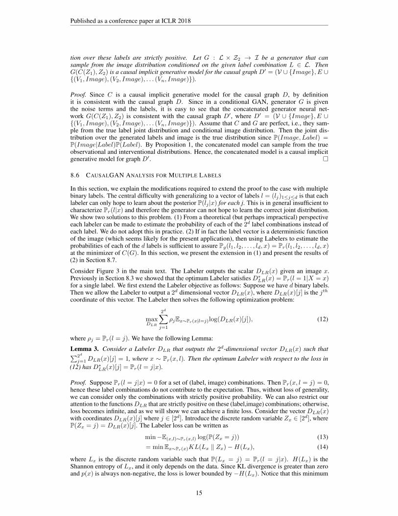
Figure 10: Synthetic data experiments: (a) Scatter plot for actual data. Data is generated using thecausal graph X1 → X2 → X3. (b) Generated distribution when generator causal graph is
X1 → X2 → X3. (c) Generated distribution when generator causal graph isX1 → X2 → X3 ∪X1 → X3. (d) Generated distribution when generator causal graph is
X1 → X2 ← X3. (e) Generated distribution when generator is from a fully connected last layer of a5 layer FF neural net.
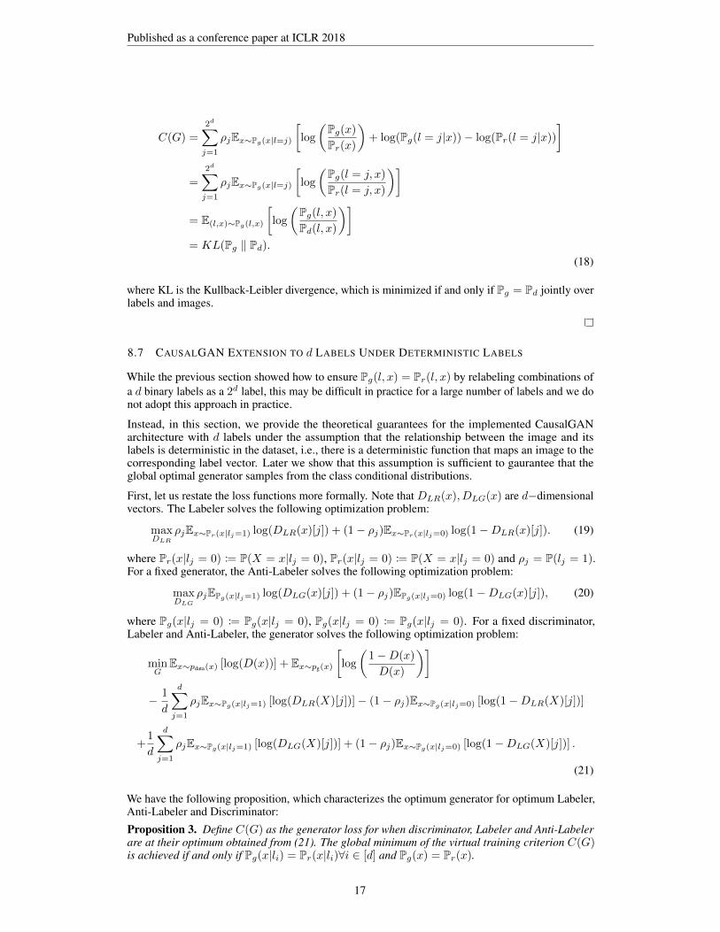
Label MalePair 0 1
Young 0 0.14[0.07](0.07) 0.09[0.15](0.15)1 0.47[0.51](0.51) 0.29[0.27](0.26)
Mustache 0 0.61[0.58](0.58) 0.34[0.38](0.38)1 0.00[0.00](0.00) 0.04[0.04](0.04)
Table 1: Pairwise marginal distribution for select label pairs when Causal Controller is trainedon G1 in plain text, its completion cG1[square brackets], and the true pairwise distribution(inparentheses). Note that G1 treats Male and Young labels as independent, but does not completelyfail to generate a reasonable (product of marginals) approximation. Also note that when an edge isadded Y oung →Male, the learned distribution is nearly exact. Note that both graphs contain theedge Male→Mustache and so are able to learn that women have no mustaches.
observe, using the correct graph gives the closest scatter plot to the original data, whereas using thewrong Bayesian network, collider graph, results in a very different distribution.
Second, we expand on the causal graphs used for experiments for the CelebA dataset. We use a causalgraph on a subset of the image labels of CelebA dataset, which we call CelebA Causal Graph (G1),illustrated in Figure 8. The graph cG1, which is a completed version of G1, is the complete graphassociated with the ordering: Young, Male, Eyeglasses, Bald, Mustache, Smiling, Wearing Lipstick,Mouth Slightly Open, Narrow Eyes. For example, in cG1 Male causes Smiling because Male comesbefore Smiling in the ordering. The graph rcG1 is formed by reversing every edge in cG1.
Next, we check the effect of using the incorrect Bayesian network for the data. The causal graph G1generates Male and Young independently, which is incorrect in the data. Comparison of pairwisedistributions in Table 1 demonstrate that for G1 a reasonable approximation to the true distributionis still learned for {Male, Young} jointly. For cG1 a nearly perfect distributional approximation islearned. Furthermore we show that despite this inaccuracy, both graphs G1 and cG1 lead to CausalControllers that never output the label combination {Female,Mustache}, which will be importantlater.
Wasserstein GAN in its original form (with Lipshitz discriminator) assures convergence in distributionof the Causal Controller output to the discretely supported distribution of labels. We use a slightlymodified version of Wasserstein GAN with a penalized gradient (Gulrajani et al. (2017)). We firstdemonstrate that learned outputs actually have "approximately discrete" support. In Figure 11a,we sample the joint label distribution 1000 times, and make a histogram of the (all) scalar outputscorresponding to any label.
Although Figure 11b demonstrates conclusively good convergence for both graphs, TVD is notalways intuitive. For example, "how much can each marginal be off if there are 9 labels and the TVD
21

Published as a conference paper at ICLR 2018
Label, L PG1(L = 1) PcG1(L = 1) PD(L = 1)
Bald 0.02244 0.02328 0.02244Eyeglasses 0.06180 0.05801 0.06406
Male 0.38446 0.41938 0.41675Mouth Slightly Open 0.49476 0.49413 0.48343
Mustache 0.04596 0.04231 0.04154Narrow Eyes 0.12329 0.11458 0.11515
Smiling 0.48766 0.48730 0.48208Wearing Lipstick 0.48111 0.46789 0.47243
Young 0.76737 0.77663 0.77362
Table 2: Marginal distribution of pretrained Causal Controller labels when Causal Controller istrained on CelebA Causal Graph (PG1) and its completion(PcG1), where cG1 is the (nonunique)largest DAG containing G1 (see appendix). The third column lists the actual marginal distributionsin the dataset
0.00.05
1.00.95
0.5
66%
0.25
0.75
30%2% 2%
(a) Essentially Discrete Range of Causal Controller
0 2000 4000 6000 8000 10000 12000 14000 16000 18000Training Step
0.0
0.2
0.4
0.6
0.8
1.0
Tota
l Var
iatio
n Di
stan
ce
TVD of Label Generationedge-reversed complete CelebA Causal Graphcomplete CelebA Causal GraphCelebA Causal Graph
(b) TVD vs. No. of Iters in CelebA Labels
Figure 11: (a) A number line of unit length binned into 4 unequal bins along with the percentof Causal Controller (G1) samples in each bin. Results are obtained by sampling the joint labeldistribution 1000 times and forming a histogram of the scalar outputs corresponding to any label.Note that our Causal Controller output labels are approximately discrete even though the input is acontinuum (uniform). The 4% between 0.05 and 0.95 is not at all uniform and almost zero near 0.5.(b) Progression of total variation distance between the Causal Controller output with respect to thenumber of iterations: CelebA Causal Graph is used in the training with Wasserstein loss.
is 0.14?". To expand upon Figure 2 where we showed that the causal controller learns the correctdistribution for a pairwise subset of nodes, here we also show that both CelebA Causal Graph (G1)and the completion we define (cG1) allow training of very reasonable marginal distributions for alllabels (Table 1) that are not off by more than 0.03 for the worst label. PD(L = 1) is the probabilitythat the label is 1 in the dataset, and PG(L = 1) is the probability that the generated label is (arounda small neighborhood of ) 1.
8.11 WASSERSTEIN CAUSAL CONTROLLER ON CELEBA LABELS
We test the performance of our Wasserstein Causal Controller on a subset of the binary labels ofCelebA datset. We use the causal graph given in Figure 8.
For causal graph training, first we verify that our Wasserstein training allows the generator to learna mapping from continuous uniform noise to a discrete distribution. Figure 11a shows where thesamples, averaged over all the labels in CelebA Causal Graph, from this generator appears on the realline. The result emphasizes that the proposed Causal Controller outputs an almost discrete distribution:96% of the samples appear in 0.05−neighborhood of 0 or 1. Outputs shown are unrounded generatoroutputs.
22

Published as a conference paper at ICLR 2018
A stronger measure of convergence is the total variational distance (TVD). For CelebA Causal Graph(G1), our defined completion (cG1), and cG1 with arrows reversed (rcG1), we show convergence ofTVD with training (Figure 11b). Both cG1 and rcG1 have TVD decreasing to 0, and TVD for G1assymptotes to around 0.14 which corresponds to the incorrect conditional independence assumptionsthat G1 makes. This suggests that any given complete causal graph will lead to a nearly perfectimplicit causal generator over labels and that bayesian partially incorrect causal graphs can still givereasonable convergence.
8.12 MORE CAUSALGAN RESULTS
In this section, we present additional CausalGAN results in Figure 12, 13.
Intervening vs Conditioning on Wearing Lipstick, Top: Intervene Wearing Lipstick=1,Bottom: Condition Wearing Lipstick=1
Figure 12: Intervening/Conditioning on Wearing Lipstick label in CelebA Causal Graph. SinceMale→WearingLipstick in CelebA Causal Graph, we do not expect do(Wearing Lipstick = 1)to affect the probability of Male = 1, i.e., P(Male = 1|do(Wearing Lipstick = 1)) = P(Male =1) = 0.42. Accordingly, the top row shows both males and females who are wearing lipstick.However, the bottom row of images sampled from the conditional distribution P(.|Wearing Lipstick =1) shows only female images because in the dataset P(Male = 0|Wearing Lipstick = 1) ≈ 1.
Intervening vs Conditioning on Narrow Eyes, Top: Intervene Narrow Eyes=1, Bottom:Condition Narrow Eyes=1
Figure 13: Intervening/Conditioning on Narrow Eyes label in CelebA Causal Graph. SinceSmiling → Narrow Eyes in CelebA Causal Graph, we do not expect do(Narrow Eyes = 1) to affectthe probability of Smiling = 1, i.e., P(Smiling = 1|do(Narrow Eyes = 1)) = P(Smiling =1) = 0.48. However on the bottom row, conditioning on Narrow Eyes = 1 increases the proportionof smiling images (From 0.48 to 0.59 in the dataset), although 10 images may not be enough to showthis difference statistically.
8.13 MORE CAUSALBEGAN RESULTS
In this section, we train CausalBEGAN on CelebA dataset using CelebA Causal Graph. The CausalController is pretrained with a Wasserstein loss and used for training the CausalBEGAN.
To first empirically justify the need for the margin of margins we introduced in (27) (c3 and b3), wetrain the same CausalBEGAN model setting c3 = 1, removing the effect of this margin. We showthat the image quality for rare labels deteriorates. Please see Figure 18 in the appendix. Then forthe labels Bald, and Mouth Slightly Open, we illustrate the difference between interventional andconditional sampling when the label is 1. (Figures 14, 15).
23
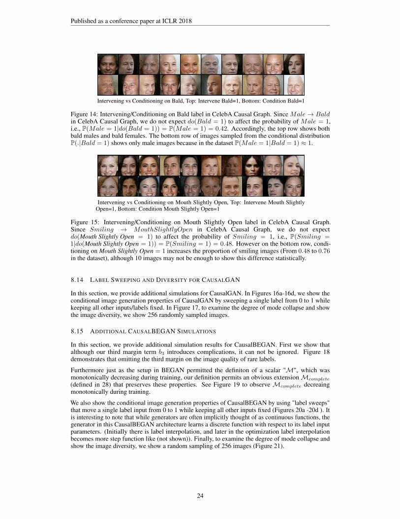
Published as a conference paper at ICLR 2018
Intervening vs Conditioning on Bald, Top: Intervene Bald=1, Bottom: Condition Bald=1
Figure 14: Intervening/Conditioning on Bald label in CelebA Causal Graph. Since Male→ Baldin CelebA Causal Graph, we do not expect do(Bald = 1) to affect the probability of Male = 1,i.e., P(Male = 1|do(Bald = 1)) = P(Male = 1) = 0.42. Accordingly, the top row shows bothbald males and bald females. The bottom row of images sampled from the conditional distributionP(.|Bald = 1) shows only male images because in the dataset P(Male = 1|Bald = 1) ≈ 1.
Intervening vs Conditioning on Mouth Slightly Open, Top: Intervene Mouth SlightlyOpen=1, Bottom: Condition Mouth Slightly Open=1
Figure 15: Intervening/Conditioning on Mouth Slightly Open label in CelebA Causal Graph.Since Smiling → MouthSlightlyOpen in CelebA Causal Graph, we do not expectdo(Mouth Slightly Open = 1) to affect the probability of Smiling = 1, i.e., P(Smiling =1|do(Mouth Slightly Open = 1)) = P(Smiling = 1) = 0.48. However on the bottom row, condi-tioning on Mouth Slightly Open = 1 increases the proportion of smiling images (From 0.48 to 0.76in the dataset), although 10 images may not be enough to show this difference statistically.
8.14 LABEL SWEEPING AND DIVERSITY FOR CAUSALGAN
In this section, we provide additional simulations for CausalGAN. In Figures 16a-16d, we show theconditional image generation properties of CausalGAN by sweeping a single label from 0 to 1 whilekeeping all other inputs/labels fixed. In Figure 17, to examine the degree of mode collapse and showthe image diversity, we show 256 randomly sampled images.
8.15 ADDITIONAL CAUSALBEGAN SIMULATIONS
In this section, we provide additional simulation results for CausalBEGAN. First we show thatalthough our third margin term b3 introduces complications, it can not be ignored. Figure 18demonstrates that omitting the third margin on the image quality of rare labels.
Furthermore just as the setup in BEGAN permitted the definiton of a scalar "M", which wasmonotonically decreasing during training, our definition permits an obvious extensionMcomplete
(defined in 28) that preserves these properties. See Figure 19 to observe Mcomplete decreaingmonotonically during training.
We also show the conditional image generation properties of CausalBEGAN by using "label sweeps"that move a single label input from 0 to 1 while keeping all other inputs fixed (Figures 20a -20d ). Itis interesting to note that while generators are often implicitly thought of as continuous functions, thegenerator in this CausalBEGAN architecture learns a discrete function with respect to its label inputparameters. (Initially there is label interpolation, and later in the optimization label interpolationbecomes more step function like (not shown)). Finally, to examine the degree of mode collapse andshow the image diversity, we show a random sampling of 256 images (Figure 21).
24

Published as a conference paper at ICLR 2018
(a) Interpolating Bald label (b) Interpolating Male label
(c) Interpolating Young label (d) Interpolating Eyeglasses label
Figure 16: The effect of interpolating a single label for CausalGAN, while keeping the noise termsand other labels fixed.
25

Published as a conference paper at ICLR 2018
Figure 17: Diversity of the proposed CausalGAN showcased with 256 samples.
26

Published as a conference paper at ICLR 2018
Figure 18: Omitting the nonobvious margin b3 = γ3 ∗ relu(b1)− relu(b2) results in poorer imagequality particularly for rare labels such as mustache. We compare samples from two interventional dis-tributions. Samples from P(.|do(Mustache = 1)) (top) have much poorer image quality comparedto those under P(.|do(Mustache = 0)) (bottom).
0 50000 100000 150000 200000Step
0.100
0.125
0.150
0.175
0.200
0.225
0.250
0.275
0.300
M c
ompl
ete
Mcomplete vs step
Figure 19: Convergence of CausalBEGAN captured through the parameterMcomplete.
27

Published as a conference paper at ICLR 2018
(a) Interpolating Bald label (b) Interpolating Male label
(c) Interpolating Young label (d) Interpolating Eyeglasses label
Figure 20: The effect of interpolating a single label for CausalBEGAN, while keeping the noise termsand other labels fixed. Although most labels are properly captured, we see that eyeglasses label is not.
28

Published as a conference paper at ICLR 2018
Figure 21: Diversity of Causal BEGAN showcased with 256 samples.
29

Published as a conference paper at ICLR 2018
Figure 22: Failed Image generation for simultaneous label and image generation after 20k steps.
8.16 DIRECTLY TRAINING CIGM FOR LABELS+IMAGE FAILS
In this section, we present the result of attempting to jointly train an implicit causal generative modelfor labels and the image. This approach treats the image as part of the causal graph. It is not clearhow exactly to feed both labels and image to discriminator, but one way is to simply encode the labelas a constant image in an additional channel. We tried this for CelebA Causal Graph and observedthat the image generation is not learned (Figure 22). One hypothesis is that the discriminator focuseson labels without providing useful gradients to the image generation.
9 IMPLEMENTATION
In this section, we explain the differences between implementation and theory, along with otherimplementation details for both CausalGAN and CausalBEGAN.
9.1 PRETRAINING CAUSAL CONTROLLER FOR FACE LABELS
In this section, we explain the implementation details of the Wasserstein Causal Controller forgenerating face labels. We used the total variation distance (TVD) between the distribution ofgenerator and data distribution as a metric to decide the success of the models.
The gradient term used as a penalty is estimated by evaluating the gradient at points interpolatedbetween the real and fake batches. Interestingly, this Wasserstein approach gives us the opportunityto train the Causal Controller to output (almost) discrete labels (See Figure 11a). In practice though,we still found benefit in rounding them before passing them to the generator.
The generator architecture is structured in accordance with Section 4 based on the causal graphin Figure 8, using uniform noise as exogenous variables and 6 layer neural networks as functionsmapping parents to children. For the training, we used 25 Wasserstein discriminator (critic) updatesper generator update, with a learning rate of 0.0008.
9.2 IMPLEMENTATION DETAILS FOR CAUSALGAN
In practice, we use stochastic gradient descent to train our model. We use DCGAN Radford et al.(2015), a convolutional neural net-based implementation of generative adversarial networks, andextend it into our Causal GAN framework. We have expanded it by adding our Labeler networks,training a Causal Controller network and modifying the loss functions appropriately. Compared toDCGAN an important distinction is that we make 6 generator updates for each discriminator updateon average. The discriminator and labeler networks are concurrently updated in a single iteration.
Notice that the loss terms defined in Section 5.2.1 contain a single binary label. In practice we feeda d-dimensional label vector and need a corresponding loss function. We extend the Labeler and
30
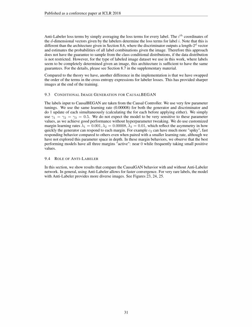
Published as a conference paper at ICLR 2018
Anti-Labeler loss terms by simply averaging the loss terms for every label. The ith coordinates ofthe d-dimensional vectors given by the labelers determine the loss terms for label i. Note that this isdifferent than the architecture given in Section 8.6, where the discriminator outputs a length-2d vectorand estimates the probabilities of all label combinations given the image. Therefore this approachdoes not have the guarantee to sample from the class conditional distributions, if the data distributionis not restricted. However, for the type of labeled image dataset we use in this work, where labelsseem to be completely determined given an image, this architecture is sufficient to have the sameguarantees. For the details, please see Section 8.7 in the supplementary material.
Compared to the theory we have, another difference in the implementation is that we have swappedthe order of the terms in the cross entropy expressions for labeler losses. This has provided sharperimages at the end of the training.
9.3 CONDITIONAL IMAGE GENERATION FOR CAUSALBEGAN
The labels input to CausalBEGAN are taken from the Causal Controller. We use very few parametertunings. We use the same learning rate (0.00008) for both the generator and discriminator anddo 1 update of each simultaneously (calculating the for each before applying either). We simplyuse γ1 = γ2 = γ3 = 0.5. We do not expect the model to be very sensitive to these parametervalues, as we achieve good performance without hyperparameter tweaking. We do use customizedmargin learning rates λ1 = 0.001, λ2 = 0.00008, λ3 = 0.01, which reflect the asymmetry in howquickly the generator can respond to each margin. For example c2 can have much more "spiky", fastresponding behavior compared to others even when paired with a smaller learning rate, although wehave not explored this parameter space in depth. In these margin behaviors, we observe that the bestperforming models have all three margins "active": near 0 while frequently taking small positivevalues.
9.4 ROLE OF ANTI-LABELER
In this section, we show results that compare the CausalGAN behavior with and without Anti-Labelernetwork. In general, using Anti-Labeler allows for faster convergence. For very rare labels, the modelwith Anti-Labeler provides more diverse images. See Figures 23, 24, 25.
31
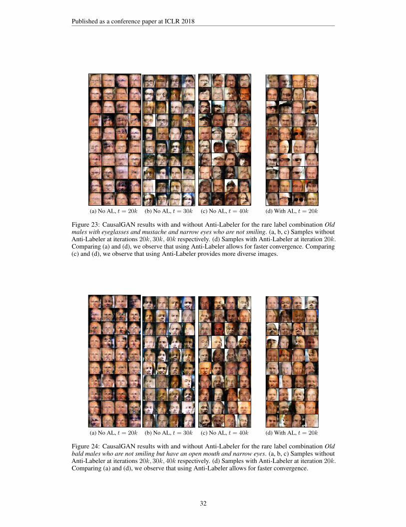
Published as a conference paper at ICLR 2018
(a) No AL, t = 20k (b) No AL, t = 30k (c) No AL, t = 40k (d) With AL, t = 20k
Figure 23: CausalGAN results with and without Anti-Labeler for the rare label combination Oldmales with eyeglasses and mustache and narrow eyes who are not smiling. (a, b, c) Samples withoutAnti-Labeler at iterations 20k, 30k, 40k respectively. (d) Samples with Anti-Labeler at iteration 20k.Comparing (a) and (d), we observe that using Anti-Labeler allows for faster convergence. Comparing(c) and (d), we observe that using Anti-Labeler provides more diverse images.
(a) No AL, t = 20k (b) No AL, t = 30k (c) No AL, t = 40k (d) With AL, t = 20k
Figure 24: CausalGAN results with and without Anti-Labeler for the rare label combination Oldbald males who are not smiling but have an open mouth and narrow eyes. (a, b, c) Samples withoutAnti-Labeler at iterations 20k, 30k, 40k respectively. (d) Samples with Anti-Labeler at iteration 20k.Comparing (a) and (d), we observe that using Anti-Labeler allows for faster convergence.
32
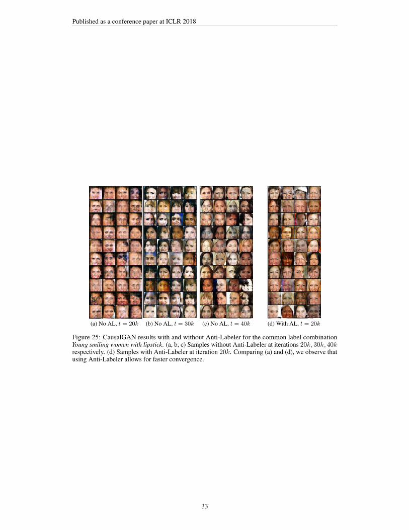
Published as a conference paper at ICLR 2018
(a) No AL, t = 20k (b) No AL, t = 30k (c) No AL, t = 40k (d) With AL, t = 20k
Figure 25: CausalGAN results with and without Anti-Labeler for the common label combinationYoung smiling women with lipstick. (a, b, c) Samples without Anti-Labeler at iterations 20k, 30k, 40krespectively. (d) Samples with Anti-Labeler at iteration 20k. Comparing (a) and (d), we observe thatusing Anti-Labeler allows for faster convergence.
33


![Journal of Big Data - RESEARCH OpenAccess ......e.g., improved classification modeling [9], better quality of generated samples by gener-ative probabilistic models [10], and the invariant](https://img.pdfslide.net/doc/110x75/6125d87877b3002268280c5a/journal-of-big-data-research-openaccess-eg-improved-classification.jpg)