~

I

NASA CR-165828 NASA-CR-165828 19820024761

ERROR NORMS FOR THE ADAPTIVE SOLUTION OF THE NA VIER-STOKES EQUATIONS

C. K. Forester

Boeing Military Airplane Company Seattle, Washington

Prepared for Langley Research Center under contract NAS 1-16408

NI\SI\ NatIOnal AeronautICS and Space AdrnrnstratJon

langley Research Center Hampton, Virginia 23665

May 1982

.- - Inn' .... : ! \, () ~ \lA,,", <

U 1'~':L=Y ~~)~[ \,":H ':LtJ fct( L,::-~~'( ;'1<','\

l-' ~ f. ~-'-JN, \11 <~II ':-\

111111111111111111111111111111111111111111111 NF01354 ~

1 R'pOtl No ·1 2 Government ~c.",on No 3 Re<:lplent. ClUI09 No

NASA CR 165828 4 T,U •• nd Subll'" 5 Report Dale

Error Norms for the Adaptive Solution of the July 1982 Navier-Stokes Equations 6 Performing Organization Code

7 Author',) 8 Perfarmor'9 OrQllnlZlllon Report No

C. K. Forester 10 Work Unit No

9 Performing O'QllnlutlOn Name and Address

Boeing Military Airplane Company P.O. Box 3707 11 Conlract or Grlnt No

Seattle, Washington 98124 NAS1-16408 13 Type of Report and Period Covered

12 SponsDtlng Ag«tcy Name and Addreu Contractor Report National Aeronautics and Space Administration Washlngton, D.C. 20546 14 SponlOflng Agencv Code

15 Supplernenury Nom

Final Report

16 AbmIct

The adaptive solution of the Navier-Stokes equations depends upon the successful interaction of three key elements; 1) the ability to flexibly select grid length scales in composite grids, 2) the ability to efficiently control residual error in composite grids, and 3) the ability to define reliable, convenient error norms to guide the grid adjustment and optimize the residual levels relative to the local truncation errors. An initial investigation was conducted to explore how to approach developing these

I key ele'T'ents. Conventional error assessment methods were defined and defect- and deferred-correction methods were surveyed. The one-dimensional potenti~l equation was used as a multi-grid test-bed to investigate how to achieve successful interaction of these three key elements. Recommendations are made for further work on error norms and enhanced residual error control for the potential and Navier-Stokes equations in a series of computer codes of i~creasing complexity. Culmination of this effort is for nested multi-grid modeling of flows with singularities or steep gradients.

17 Key Word' (Suggened by Author(s)) 18 DiStribution Slale'TII"t Partial Di fferent i a 1 Equations Navier-Stokes Equations Numerical Solution Methods Numerical Error Assessment Multi-arid and Defect Corrections I

19 SeeUflty Cassl! (o! thiS report) 120 Security Ousil (01 thl' pagel 121 No 01 Pagfl 122 Pnce'

I Uncl assified Unclassified

• For sale by the National Technical Inforr;;atlo~ Se'vlce Springfield VI,glnta 22161

~ASA-C·168 (Rev 10.iS)

ERROR NORMS FOR THE ADAPTIVE SOLUTION OF THE NAVIER-STOKES EQUATIONS

C. K. Forester

Boeing Military Airplane Company Seattle, Washington 98124

for

NASA Langley Research Center Hampton, Virginia

Contract NASl-16408

TABLE OF CONTENTS

NOMENCLATURE

LIST OF FIGURES

1.0 SUMMARY

2.0 INTRODUCTION 2.1 Objectives of the Study 2.2 Technical Approach

3.0 NUMERICAL CONSIDERATIONS 3.1 Typ~s of Error Sources

3.1.1 Mathematical Description 3.1.2 Truncation Errors 3.1.3 Filtering and Damping 3.1.4 Residual Errors

3.2 Error Assessment and Control 3.2.1 Conventional Certification 3.2.2 Engineering Approaches 3.2.3 Error Norm Approaches

3.2.3.1 Conventional Error Norms 3.2.3.2 Taylor Series Error Monitor 3.2.3.3 Variable-Order-Accurate Algorithms 3.2.3.4 Multi-Grid Error Norms

4.0 NUMERICAL ANALYSIS AND RESULTS 4.1 Solution of the 1-0 Potential Equation 4.2 Solution of the 1-0 Potential Equation with Multi-Grid 4.3 Test Problem 4.4 Error Norm Evaluation 4.5 Adaptive Grid Example

i

PAGE

iii

iv

1

3 5

5

7 7 7 8 9

10 10 11

13 14 14 16 16

18

20 20 23

26

28

31

TABLE OF CONTENTS (concluded)

5.0 DISCUSSION 5.1 Error Assessment 5.2 Multi-Grld 5.3 Control of the Length Scales for Steep Gradient Reglons

6.0 CONCLUSIONS

7.0 RECOMMENDATIONS

8.0 REFERENCES

ii

PAGE

33

33

34

37

39

40

42

NOMENCLATURE

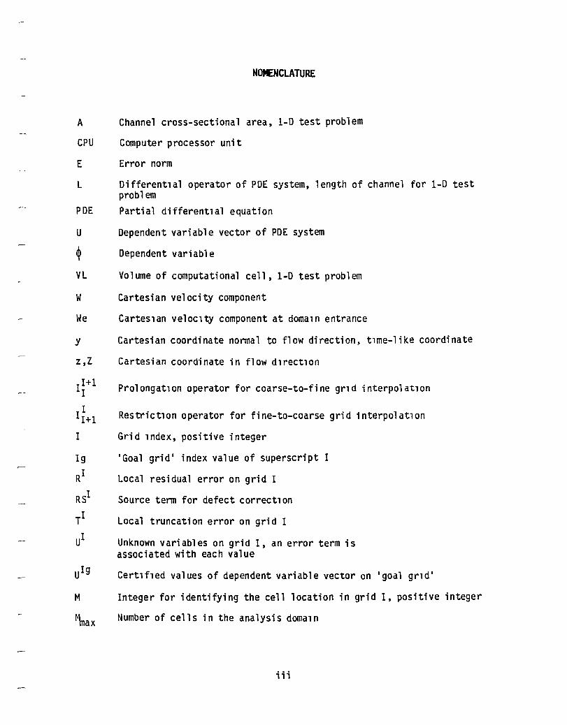
A Channel cross-sectional area, 1-0 test problem

CPU Computer processor unit

E Error norm

L Differentlal operator of POE system, length of channel for 1-0 test problem

POE Partial differentlal equation

U Dependent variable vector of POE system

~ Dependent variable

VL Volume of computational cell, 1-0 test problem

W Cartesian velocity component

We Carteslan veloclty component at domaln entrance

y Cartesian coordinate normal to flow direction, tlme-like coordinate

Z,Z Cartesian coordinate in flow dlrectlon

1~+1 Prolongatlon operator for coarse-to-fine grld interpolatlon

I 11+1 Restrictlon operator for fine-to-coarse grid interpolatlon

I Grid lndex, positive integer

19 'Goal grid ' index value of superscript I

RI Local residual error on grid I

RSI Source term for defect correctlon

rI Local truncation error on grid I

UI Unknown variables on grid I, an error term is associated with each value

uI9 Certlfled values of dependent variable vector on 'goal grld '

M Integer for identifying the cell location in grid I, positive integer

~ax Number of cells in the analysis domaln

iii

1.

2.

3.

4.

5.

6.

LIST OF FIGURES

One-dimensional Incompressible Channel Flow

Residual Error Effects on Fixed Grid and Multi-Grid Solutions

Truncation Error Effects on Intermediate Grid Level Solutions

Truncation Error Spectrum as a Function of Grid Density

Why Brandt's Coarse-to-Fine Grid Correction Equation is Needed

Adaptive Grid Control to Selected Truncation Error Tolerance

iv

PAGE

44

45

46

47

48

49

1.0 SUMMARY

The current practice for applied analysis in the aerospace industry is to use specially selected combinations of coupled zonal models - inviscid, shear layer, etc. - to approximate the field equations of fluid mechanics for various applications.

partial differential

The zonal models involve systems of ordinary and equations (field equations). These equations are

simulated with numerical methods which possess two types of numerical errors -residual errors and truncati on errors. Residual (sol uti on process) errors arise due to insufficient iterations of implicit algebraic equations by relaxation or the inversion of ill-conditioned matrices. Truncation (grid related) errors arise due to the selection of the grid, the grld-re1ated algebraic equations and the associated boundary and initial conditions. Residual errors and truncation errors can be very significant. Assessing the effects of numerical error on the modeling of the field equations is a tedious and expensive process involving parametric cycling through various tolerances on residual error and various grid densities and distributions. Grid 1ength­scale control to properly resolve shock and shear layer singularities is unava i 1 ab 1 e except for speci a 1i zed cases. Because of these di ffi cu1 ti es , numerical error effects are not commonly examined or controlled with precision using conventional methods of numerical analysis, and this can lead to a misinterpretation of computed results.

Efficient solution of the equations of fluid mechanics requires the availability of adaptive mesh generation and numerical error assessment methods to define numerical errors and guide the grid adjustment process. The overall goal of this research program is the development of these methods.

The obj ecti ves of the work reported herei n were to begi n development of algorithms to define error norms (for use as resolution monitors) for numerical solution of POE's and to begin development of a multi-level adaptive grid technique for application to the solution of the various equation sets used to model fluid flow. The present work is an inltia1 exploratory investigation of resolution monitors and adaptive grid technology.

1

The approach was as follows. multl-grid methods was briefly

The llterature on error assessment ana reviewed. From this, conventional error

assessment methods were defined and are brlefly described. Three variable­order-accuracy defect-correction approaches were identified. The one-dlmensional (1-0) incompressible potentlal equation was selected as a test bed to investigate error assessment and multi-grid methods. A test problem, a channel wlth a constrlctlon, was selected for WhlCh analytic Solutlons were available. The equation was solved for the test problem using point

relaxation for a range of mesh densitles and distributlons and the varlOUS error assessment techniques were evaluated. The test problem was also solved uSlng point relaxation and a multi-grid scheme and the characterlstlcs of the multi-grid method were evaluated.

One result is that multl-grid schemes are promising as a basis for developlng resolution monitors and adaptive grid techniques. Brandt's methodology appears to be the most suitable approach to adaptive-grld-control. The present study suggests that the multi-grid technology is conceptually straightforward to apply to conventional computer codes WhlCh solve elliptlc problems. A second is that for the test problem, reliable estimates of the maximum glooal error were obtained from solution output for a number of grld levels. From the work completed, it is expected that substantial improvements are posslble for assesslng and controlling numerlcal errors. A thlrd result is that slgnificant improvement for efficlent residual error control was demonstrated with the test problem. Further work is, however, requlred to develop the three key elements: (1) error norms to guide grid adjustment for truncation error control, (2) methods for efflclent resldual error control (relaxatlon schemes that work well with irregular mesh intervals), and (3) adaptive mesh structures based on these error norms. The efflcient interaction of these three key elements is necessary to obtain adaptive Solutlon of the Navier-Stokes equatlons.

A follow-on research program is recommended which addresses development of the three key elements deflned in the work reported herein and noted above. The development of these elements would occur simultaneously, utilizing a series of research computer programs of increaslng complexlty.

Work reported herein was supported by NASA contract NASl-16408 and Boeing IR&D funds.

2

2.0 INTRODUCTION

The Navier-Stokes equations with continuity, energy and state equations are the accepted analytical model for fluids whose constituative properties are Newtonian. They apply to the flight envelope of most aircraft in the earth's

atmosphere and to all steady and unsteady laminar and turbulent flow processes which influence the performance of these aircraft. The development of numerical techniques to model the Navier-Stokes equations has been revolutionary in recent years and the pace is accelerating.

The Navi er-Stokes equations are always simpl ified to rel ated but di fferent partial differential equations (POE). These simplified POE systems are chosen to model the essenti a 1 properti es of the Navi er-Stokes equati ons for the intended application. In the solution of many of these flows, it is difficult to sort out modeling errors from numerical errors. An obvious example is the use of the Reynolds averaged Navier-Stokes equations for turbulent flow.

Selecting appropriate PDE systems depends upon havlng an understanding of the PDE solution properties. These are defined through analytica:l and numerical methods. POE modeling depends upon understanding the numerical results including distortions induced by numerical errors. It is important to control these numerical distortions to within tolerances that are consistent with the intended application. The cost to achieve a given level of accuracy is also important. The cost/benefit relation must be readily accessible, otherwise unrealistic levels of accuracy may be demanded without real benefits or insufficient accuracy may occur with misleading results.

The present effort is di rected at the physics of smooth steady flows wi th interacting singul arity regions such as shocks, boundary 1 ayers, free shear layers, flame fronts and contact surfaces. Existing solution techniques for the equations describing these flows are usually unable to control the length scales of the mesh in these singularity regions sufficiently to accurately resolve these flow features because they are inefficient at the necessary grid scales. As a consequence, computed results are of low accuracy.

3

Efficient numerical model ing of these equations Wl th systems of algebraic equations for a grid is difficult because of residual errors in the solution process and truncation errors. Resldual errors occur because of the Gibbs' effect (wiggles or high frequency oscilla~ions in the solution) and the stiffness of the equati ons (acousti c, diffusi ve and convecti ve stiffness). Stiffness is defined as slow convergence toward the target of zero residual errors. Truncation errors are due to the grld selected, the grld related

algebraic equations solved, and the boundary and initial conditions - all used to approximate the field equations in an analysis domain. These problems are compounded by the grid requirements of singular flows; grid length scales are needed near singularities that vary by orders-of-magnitude from those required in regions of low gradients in flow properties.

Algorithms for numerical solution of the Navier-Stokes equations are sought which address simultaneously the requirements for

a. grid related algebraic solution procedures for improved reduction of residual errors

b. error monitors that efflclently asslst the grid adJustment process and optimize the residuals relative to the truncation errors

c. solution procedures WhlCh are less sensltlve to mesh and permit grld nesting.

Adaptive grid control is the interaction of these elements to reduce numerlcal error. Manual and automatic processes can be used to implement adaptivity. A balance between computer code development time and computer code user complexity must be kept in mind.

1 1· ,(1) . The multi- eve adaptlVe grid procedure produces truncatlon error

estimates as a by-product of the solution procedure which could be used as a resolution monitor. This procedure is thus especially attractive as an approach to the development of automatic POE solvers which control numerical errors to a prescribed tolerance.

Work reported herein was supported by NASA Contract NASl-16408 and Boeing IR&O.

4

2.1 THE OBJECTIVES OF THE STUDY

The first goal of the research is the development of numerical error assessment methods for use as gr1d resolution monitors. The second goal is adaptive mesh generation methods to refine the grid locally where indicated by the resolution monitor. The third goal is to improve the efficiency of resi dual error control with non-uni form meshes. It is expected that the availability of this technology will provide significant improvement in the numerical solution of the PDE's of fluid mechanics. Substantial work is necessary before this will be possible. The objectives of the present work were to begi n development of a 1 gori thms to defi ne error norms and to begi n development of mUlti-level adaptive grid techniques.(l) The present work is an initial exploratory investigation of resolution monitors, grid adjustment methods, and residual error control efficiency.

2.2 THE TECHNICAL APPROACH

Two overall strategies are being used to guide the development of resolution monitors and adaptive grid methods. The first strategy is to define as early as possibl e all of the el ements necessary to the development of the desi red technology and to address these simultaneously. The second is to use simple one-dimensional numerical "test beds" to define and develop the necessary technology elements. Once the technology elements are defined and developed, extension of the technology to test bed codes for 2-D and 3-D POE's of fluid mechanics should be relatively straightforward. With this background, the error-norm adaptive grid technology can then be applied to codes for efficient solution of fluid flow analysis problems.

Specifically for the work reported herein the detailed technical approach was as follows:

1) The 1 i terature on error assessment and mul ti -gri d methods was bri efly reviewed. Error sources were identified, Section 3.1, and a brief mathemati cal descri pti on of these is presented in Secti ons 3.1.1 and 3.1.2. Control of numerical error with filtering and damping and the necessary interaction with error assessment methods are described in

5

Section 3.1.3. The problem of efficient residual error control is discussed in Section 3.1.4.

Conventional approaches to error assessment and control are di scussed in Section 3.2. Three approaches were identified; the conventional

certification process, Section 3.2.1, the engineering approaches, Section 3.2.2, and the error norm approaches, Section 3.2.3.

Four error norm approaches to numerical error assessment were 1 dentlfied. Conventional error norms are defined in Section 3.2.3.1. A Taylor series error monitor approach is described in Section 3.2.3.2. Variable order accuracy algorithms for error assessment are described in Section 3.2.3.3. Multi-grid error norms are then described in Section 3.2.3.4.

2) Solution of the one-dimensional potential equation was selected as a test bed to investigate error assessment and multi-grid methods, Section 4.0. Numerical solution of the potential equation using point relaxation is described in Section 4.1 and using point relaxation and a multi-grid procedure, in Section 4.2.

3) The test problem was solved using the point relaxation and the multi-grid scheme as described in Section 4.3.

4) The various error norms were evaluated as described in Section 4.4, and an adaptive mesh example is presented in Section 4.5.

5) Computed results were evaluated and are discussed in Section 5.0.

6

Conclusions and recommendations for further work are suggested in Section 6.0 and 7.0.

3.0 NUMERICAL CONSIDERATIONS

3.1 TYPES OF ERROR SOURCES

The numerical methods for solving PDE's have two types of error sources: gri d-rel ated sol uti on process (resi dual) errors and gri d-p1 acement re1 ated (truncation) errors. Explicit marching techniques (time or space) do not have residual errors unless there is an implicit equation imbedded in the marching scheme. Residual errors occur when implicit equations are solved by explicit

marching techniques, specialized relaxation schemes or matrix inversion processes. Only i deal difference schemes have no truncati on-error effects.

Practical flow analysis tools are not ideal. Truncation-error and residual-error effects produce many curious phenomena which must be understood in order to develop reliable error norms. The error norms must be able to detect any spurious or peculiar numerical phenomena.

3.1.1 Mathe.atical Description

Let LU = 0 3.1.1-1

represent the POE system of interest.

In discretized operator notation, equation 3.1.1-1 is

3.1.1-2

where LI is the discretization operator, UI is related to the discretized dependent variable vector, and TI is the local truncation error and RI is the local residual error for each cell of the analysis domain. The grid structure index, I, is related to choices of the grid density distributions for each selected trial grid where in general the computational grid features coupled conformal grids with grid nesting in sub-regions. Ideally the grid adjustments are made in some pattern that tend toward a limiting grid configuration or 'goal grid. ' Thus each unique grid shape is represented by

-an integer value of I. The 'goal grid ' is assigned the index Ig, which is known once the numerical error has been constrained to the desired bound.

7

An ideal or perfect difference scheme for 3.1.1-2 is one in WhlCh the local truncation error does not contaminate the variables of interest, such as velocity, density, pressure, etc. Only the residual errors impact these variables. Thus, the user specifies exactly the locations in the geometry at which values of these variables are deslred. Wlth resldual error control within adequate bounds, the accuracy of the result is insured within selected 1 imits.

Non-ideal difference schemes are defined as those in WhlCh tne local truncation error and residual errors simultaneously influence the value of the decoded variables. Except for specialized difference schemes for model problems, difference schemes for conventional applied analysis are non-ideal. Control of both error sources is addressed herein with emphasis on controlling the truncation error. This subject is closely related to the problem of proper grid adjustment from an initial state to the I goal grid ' state, with p~oper residual control during the grid-adjustment process.

3.1.2 Truncation (Grid Related) Errors Truncation errors are due to the selection of the grid, the grid related algebraic equations, and the boundary and initial conditions which approximate the field equations of interest.

The local truncation error is formally defined as the magnitude that the left-hand side of (3.1.1-2) yields for each cell when the 'goal grid ' solution is interpol ated (restri cted) to a trlal gri d difference equati on mi nus the interpolated value of the left-hand side of (3.1.1-2) from the 'goal grid ' • It is set at zero in conventional representations of (3.1.1-2) for all values of 1. In the defect- and deferred-correction methods discussed in Sections 3.2.3.3 and 3.2.3.4, truncation error estimates are used to correct for truncation error effects. The right-hand side of equation (3.1.1-2) can also be a high-order accurate truncation error correction.

8

3.1.3 Filtering and Damping Spurious Numerical Waves The linear wave equation is

u + U = 0 y Z

This equation exhibits many of the features of the convection tenns of Navier-Stokes equations but it is simple enough that the powerful methods of linear analysis apply. Such analysis indicates that all the numerical methods that have been applied to model this equation have the following properties: Contro 1 of the phase errors, amp 1 i tude error and the Gi bbs-effects errors ( 2) within selected accuracy bounds depends upon the proper grid density selection per period of propagation for wavelengths of interest and with properly designed Gibbs-effects filters. Truncation errors have an accumulative effect upon the accuracy.

Gi bbs-effects errors are hi gh frequency osci 11 ati ons near the juncture of sharp changes in gradients. For the linear case, the Gibbs' error wavelength is about four, seven, sixteen and infinite (zero Gibbs effect) mesh intervals for eighth, fourth, second, and first order accuracy convective difference schemes, respecti vely. For nonl inear cases such as near shocks, the wave length of the Gibbs-effect error is about two mesh intervals for most schemes of all orders of accuracy above two. Wavelength smoothing(2) is very effective for controlling the amplitude of the Gibbs effect to within chosen bounds without introducing global damping. Low order accurate Gibbs-effects filters are especially useful for providing the global damping that is necessary for removing transient waves from certain types of relaxation processes. When properly tuned for the most effective use of the grid, the low order accurate fil tering devices whil e servi ng to adequately damp the global waves may not provide sufficiently for the control of the Gibbs' oscillations within desired bounds. Wavelength filtering in addition to the global damping is well suited to the control of the Gibbs' oscillations within desired bounds because the smoothing can be localized as desired.

Intelligent use of smoothing is one of the central difflculties of modeling transient and steady state analysis involving mixed elliptic/hyperbolic equations. Where analytical solutions are unavailable, the error nonns for analysi s of requi red accuracy must account somehow for the phase, ampl itude

9

and Gibbs-effects errors. The question whether the solution processes must be

free of Gibbs-effects errors should be treated in future work?

Dissipative and non-dissipative convective difference schemes permit expansion

shocks, artificial gross separation, etc. to form under certain conditions.

Artificial diffusion is added to eradlcate the expansion shocks. Tuning the

artificial diffusion coefficients for peak accuracy is troublesome. The goal

of the tuning process is that the artificial diffusion must decay globally and

locally with mesh refinement so that the accuracy of the sonic line shape and

position increase with mesh refinement. The error norm used must ensure this.

3.1.4 Residual Errors

The numeri ca 1 model i ng of the potenti al equati on or of the NaVl er-Stokes

equations leads to algebraic forms in which the propagation of signals is

retarded as the grid density increases. This stiffness problem leaas to

inefficient reduction of residual errors among the simultaneous system of

algebraic equations, often leading to exponential or power function decrease

in convergence as the grid density increases. Typically diffusive stiffness

is evi dent in potenti a 1 flow codes. In Navl er-Stokes codes, three Stl ffness

probl ems can appear simul taneously or separately - acoustic, convective, or­

diffusive stiffness and can be aggravated by non-uniform grid. Any or all of

these factors can undermine the convergence rate severely and can enlarge errors substanti ally. The error moni tors must be desl gned to detect slow

convergence or inefficient residual error control. For some error norms this is a severe requirement. When the local residual error is reduced to some

fraction of the local truncation error, further reduction of the residual is

not cost effective; determination of this fraction is a subJect for further

study.

3.2 ERROR ASSESSMENT AND CONTROL

Three approaches are used to assess the accuracy of POE modeling. The first

is to construct an error difference table with solutions on trial grids of

various mesh densities and distributions. The second is the use of auxiliary

information such as experimental data and related analytical solutions for various regions of the analysis domain, and the third is the use of the local

truncation and local residual error estimates associated with suitable error

norms and error bounds. These three are referred to as the conventional,

10

engineering (analogical) and the error-norm approaches to certifying the accuracy of POE modeling. Direct numerical evidence of the accuracy of the POE model ing results from the conventional and error-norm approaches. These methods have their origins in numerical analysis technology. In the engineering approach no attempt is made at achieving direct evidence. Inferential reasoning is predominately used. Discussions of this are given in the following sections.

3.2.1 Conventional Certification Process The process of numerical error assessment with conventional POE modeling techniques is the following.(3) A solution of finite difference equations (simultaneous system of algebraic equations) for a specific discretization of

the analysis domain is generated for different choices of grid density and grid distribution in the analysis domain. It is common to use a sequence of

grids of the same grid distribution that differ in grid count in each independent variable direction by factors of two -- 2, 4, 8, 16, 32, etc. The

coarser grids can be generated by deleting every other point of the finer grids. The effects of the choice of grid distribution are examined by choosing sequences of grids which have different mesh distributions. The data from all of these solutions of the grid-related equations is organized by constructi ng an error di fference tabl e. Sol ution differences are posted in order of the coarse-to-fine grids for each grid sequence. The solution differences are generated by subtracting the values of adjoining pairs of grid solutions of the dependent variables at all physical locations in the analysis

domain that correspond to the grid coordinates of a grid of a selected intermediate density. Interpolation is used to relate other grid solutions to these sel ected gri d coordi nates. As the gri d densi ty increases the differences should decay approximately* according to the formal order of accuracy for some selected mesh distribution. Iterative adjustment of the grid distribution and density is made until this type of error decay is realized. If this occurs, extrapolation may be used to solutions at infinite grid density and reliable estimates of the maximum global error may result.

*Error decay according to the formal order of accuracy is expected globally

but not locally in regions of singularity.

11

The preceding process appears to work best on the modeling of parabol ic and ell iptic equations in smooth domains with smooth boundary conditions. For mixed elliptic/hyperbolic systems, erratic results may occur due to unresolved singularity regions and/or poor residual error control, and/or Gibbs I error effects.

A key feature of this method is that grid adjustments are made in some pattern that tends toward a limiting grid configuration. A way to think about this is to define a goal grid to which the selected grid sequences must evolve. The 'goal grid ' is a grid upon which the solution is sought to some specified error bound. It should be understood that the 'goal grid ' may not be unique because of grid initialization, grid generator, and grid-equation solver properties. It is assumed that adequate control of the residual error effects has been maintained in the process of assessing the truncation error effect. This is done by developing a sequence of several solutions on each grid choice with various choices of constraints on the residual tolerances that are used to terminate the computations for each solution on that grid. Because of the need to assess the contamination by residual error, the 'goal grid ' may not be the grid of greatest density but it will have the correct shape.

Conventional techniques for developing the data necessary to certify the accuracy of numerical modeling procedures are limited by the following factors:

12

1) Costs.

2) Because of (1) above, a very limited number of solutions and thus sparse information are usually available from which error estimates can be constructed.

3) Because grid adjustment to control the error within desired bounds is cumbersome or impractical, arriving at proper grid configurations in mesh density and distribution is also difficult or impractical.

4) Numerical error during grid refinement may vary erratically, not monotonically with grid density. Confusion as to grid adjustment needs can result.

5) The software is usually not available for conveniently constructing the

error table. This means that the error assessment process is manpower

intensive. These factors di scourage development of the I goal gri d I

solution. Without this, the accuracy of the result is unknown; the

meaning of the resul tis undefined and useless unl ess appropri ate external information (user experience) is applied to the result.

The certificati on process with conventi onal computer codes util i zes error

information from many grid densities and grid geometries. This is a

multi-grid process albeit a very cumbersome and inefficient one. For the

present purposes thi s technology wi 11 be referred to as fi xed gri d (FG) even

though it is not, when properly used for numerical error assessment. It is

called FG because that is the manner in which it is used in applications; the error term associated with each number in the output is set to zero and this

is often ignored in the use of the numbers from the output.

3.2.2 Engineering Approaches Judgement in engineering applications as to what grid should be selected for

numerically model ing a POE system is often based upon an exterior body of

kAowledge(3) rather than direct numerical evidence. For example,

boundary-layer analysis can be performed with finite difference and related

analysis tools. Mesh refinement studies and conventional error norms can be

used to defi ne the accuracy and grid-choice rel ationships. Simil ar studies

can be performed on free shear layer and inviscid model problems with

analytical solutions to establish the accuracy and grid-choice relationships.

The various component features of the physics of the POE system can be studied

in this manner. The selection of the trial grid for the POE system of

engineering interest can be made upon the b~is of the physics that is

expected in each flow region of the analysis domain. The grid selection in

the various flow regions of the analysis domain can reflect the desired

accuracy that is required locally and globally for the purposes of the

analysi s. Interpretation of the resul ts of numerically model 1 ed POE systems

involves qualitative aspects of the solution. Inspection is used to insure

that solution features such as wall shear stress, wall boundary layer, free

shear layer, inviscid structure, or shock structure characteristics occur

13

where they are expected. The success of thlS approach depends on the knowledge and skill of the analyst and the time allotted for the analysis. Important physi cal processes may be inadvertently 1 gnored because numeri ca 1

errors mask solution properties. For example, artificial diffusion can be interpreted as turbulent diffusion.

Another approach to grid selection is used in engineering applications as well and sometimes augments the above approach. It i nvol ves the compari sons of computed and experimentally measured flow properti es. Gri d and local and global numerical smoothing adjustments are used to generate favorable agreement between the computed and measured flow properti es. Where experimental data is available, this approach is preferred to those that are described above and it encourages the use of analysis for predictive purposes where favorable agreement occurs.

In engineering approaches, direct numerical evidence is not used to understand the nature of the numerical properties; rather inferential and analogical reasoning are used.

3.2.3 Error Norm Approaches Four possible methods are considered here. The first method is a brlef review of conventional error norms; the second is the use of truncated Taylor series expansions for an error monitor; the thlrd is the use of variable order accuracy al gori thms; and the fourth is the mul ti -gri d approach. These are discussed below.

3.2.3.1 Conventional Error Nor.s Standard error norms(4) include:

14

E1 = [ ~(.I _ ~I1)1]/N

E2 ~ [E(~I _ ~I1)2/ (.I)2]1/2

Emax = [I(~I - ~I1) /~~ ]max ~ :: amplitude

3.2.3.1-1

3.2.3.1-2

3.2.3.1-3

where ~I is the dependent variable of the analyt1cal solution restricted to

the coordinate location of grid point 1. N is the number of grid points. ~ 11 is the d1 scretlZed sol Ut1 on on gri d 1. The sums denote component sums

in 2-0 and 3-0 situations. E1' E2, and Emax are known as the average error, the root-mean-square (rms) error and the maximum global error, respectively. The ~ax norm is best applied to non-singular problems (no shocks, shear layers, or geometry discontinuities) with smooth boundary conditions although it can be used if the regions of steep gradients are excluded. E1 and E2 are used for singular perturbation problems including the steep gradient regions. The use of these def1n1tions as written depends upon knowing ~I which is not available for cases of general interest. However, modified forms of these relations may be considered.

For example, equat10ns 3.2.3.1-1 through 3.2.3.1-3 can be given by:

EP,I2 = [ 1:1($12 _ ~11)\G(Z) ]/N

E2

I1 ,I2 = [E(($I2 _ ~Il)2/(~I2)2)]1/2

E11 ,I2 = [G(Z)j(th I2 _ ~I1) /m \12, max ~ ~ imax

,nI2 . ,n11+l 11+2 where. 1S any of, , 0 ,

3.2.3.1-4

3.2.3.1-5

3.2.3.1-6

~I2 is also regarded a

higher order accurate solution on grid Ii. G(Z) is a weighting factor which may be used to exclude regions in the analysiS domain where the local truncation error estimates exceed a selected threshold value. N is the number of cell sin the summati on. These error norms shoul d be of general use for understanding the role of residual and truncation errors, especially when used

with the error norms discussed below.

There are error estimators in addition to the ones listed above which should be considered in any application of interest. For example, certain components

of POE systems requ1re that kinetic energy, mean vortic1ty, total pressure, entropy, mass, etc. should be conserved. Oiscretized forms of these integral relations could be constructed which are relevant to the applicat10n of interest.

15

3.2.3.2 Taylor Series Error Monitor The idea of using truncated Taylor serles expanslons for an error monltor has been explored and conclusions about the cost effectlveness of such a development are summarized as follows. Consider a simple harmonic function such as the y=sin x. From calculus, the derivatives of all orders exist. The odd-order derivatives vanish when the modulus of the even-order derlVatives are maximum. At the least, pairs of odd-order and even-order derivatives would have to be approximated by flnite difference expressions to prevent

spuri ous decay of hi gher-order terms in any proposed error moni tor. The second requirement is that, in regions of the grid with long wavelength variations of a dependent variables of interest, it must establish how many pairs of odd and even orders are required to certify the numerical accuracy of the POE modeling. The third requirement is that, since high frequency oscill ations (two mesh interval 1 imit) can exci te two mesh interval

oscillation on all discretized derivative of the order of two and above, this information must be used somehow to sort GibbS errors, geometric discontinuities, etc. While the Taylor series error monitor idea is i ntri gui ng, it has conceptual and impl ementati on problems. The next secti on describes a related but perhaps better approach to error assessment.

3.2.3.3 Variable Order Accuracy Algorithms for Numerical Error Assessment* Rather than using only mesh refinement to assess numerical error, it is conceptually reasonabl e to define numerical al gori thms of variabl e order of accuracy from which direct error estimates emerge for a given grid. A way to think about this is to define a sequence of higher order accurate discretized solutions on the same grid each of which satisfy a certain smoothness property. The higher order accurate solutions on the grid are regarded as the trial analytical or reference Solutlons. The lowest order accurate solution

is regarded as the approximation. The error estimate is performed with conventional error norms. The error norms of Section 3.2.3.1 are slightly modified for error assessment by using higher order accurate solution data in place of the 12 finer grid data. Iteration can be used to determine how high

*

16

Oefect- and deferred-correction schemes are closely related because error estimates are used to improve the efficiency of residual error control. Both methods are multigrid methods.

the order of accuracy must go for reliable error estlmates. Grid adJustments are needed to provide the highest order accurate scheme with sufficient grid to meet desired accuracy bounds.

To implement the above process, a convergent variable order of accuracy algorithm approximating the POE system of interest must be available. For the boundary layer equations, Wornom(5) presents an approach. Forester(2) suggests a method for mixed hyperbolic/parabolic POE systems using odd-degree splines although other basis functions can be used. The order of accuracy of this scheme is selected simply by choosing the appropriate coefficlent matrix that is associated with the desired accuracy. With this method, orders of accuracy six, ten, fourteen, nineteen, etc. are possible and they are

activated by an input control function. Interpolation is used to initialize successive solution processes of higher accuracy.

Lindberg(6), Pereyra(7) and Stetter(S) have developed an approach which

is related to the one described above but in which certain simplifications are implemented. Basically Lindberg uses a low order accurate approximation to the POE system with a non-zero right-hand-side term that is lagged in the iteration process. This perturbation operator is a discretization (usually fourth order) of the POE system.

high-order-accurate The data for the

perturbation operator is derived from the low order of accuracy di screte equation system solution. The perturbation equation is repeatedly solved until some convergence criterion is satisfied. The output of the perturbation equation is a correction parameter. It is added to the low order of accuracy solution to yield a fourth order accurate solution at convergence. Error estimates are produced with conventional error norms by using the high-order­accurate solution as an exact representation of the POE system. The low order accurate resul t represents the approximate sol uti on. Li ndberg presents many exampl es of the effi ci ency of thi s defect-correction procedure to reduce residual and truncation errors. Success is not universal with hyperbolic problems, however, when some smoothness property is violated. It may be

inferred from Lindberg's data that if sufficient smoothing is applied to regions of rapid change in gradient, convergent results are achieved. To make Lindberg's scheme useful for hyperbolic systems, empirical studies would have to be performed to develop cri teri a for how local the smoothi ng must be constrained so that the global errors are definable. See Section 5.3 for related discussion.

17

The approaches of references (1-8) presume that some sort of mesh refinement

process toward the 'goal grid ' is used. The accuracy of these error estimators improves dramatically as the accuracy moves toward the one percent error range. They are useful gui des for gri d refi nement when errors are larger than ten percent but are not precise in the predicted magnitude. These approaches are promising for modeling mixed parabolic/elliptical/hyperbolic systems of equations but are difficult to implement when grid nesting is required.

Another approach to defect-correction has been proposed by Brandt(9). This approach suggests vari abl e order of accuracy, nested gri ds, ennancement of residual control efficiency and the efficient generation of an error term that may be useful for numerical error assessment. This approach has been called the multigrid method but it is misnamed since all numerical assessment and control schemes are multigrid.* Many variations of this methodology are possible. Most examples of this approach(l,a,lO) are for residual control

efficiencies near theoretical limits with uniform grid intervals. Irregular grids (nested grids) have yet to be widely addressed in this method.

3.2.3.4 Multi-Grid Error Norms Modifications are suggested in Section 3.2.3.1 to conventional error norms for assessing numerical error schemes. This is applicable to the FAS-MG (Full Approximatl0n Storage-Multi-Grid) scheme with one exception. The solution data at each grid level must be saved before finer grid levels are invoked in the multi-level solution process. This approach insures that the targets of residual and truncation errors are zero in the output for the various levels of grid. If this is not done, solution errors may appear on coarser grlds when in fact none exist.

The FAS-MG scheme estimates local truncation error by interactlng coarse and

fine grid solution data. Brandt suggests that the weighted integral

ET = IG(z)IT(z)ldZ 3.2.3.4-1

* Brandt's approach could be called defect-correction multi-grid or Tau multi­grid, TMG.

18

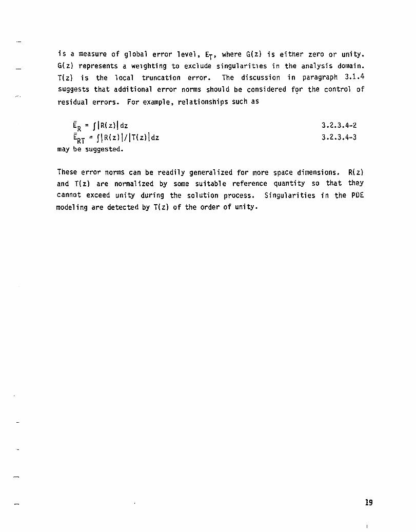
is a measure of global error level. ET• where G(z) is eitner zero or unity. G(z) represents a welghting to exclude singularitles in the analysis domain. T(z) is the local truncation error. The discussion in paragraph 3.1.4 suggests that additional error norms should be considered f9r the control of

residual errors. For example. relationships such as

ER = IIR(z)\dz ERT = J\R(z)\/\T(z)\dz

may be suggested.

3.2.3.4-2 3.2.3.4-3

These error norms can be readily generalized for more space dimensions. R(z) and T(z) are normalized by some suitable reference quantity so that they cannot exceed unity during the solution process. Singularities in the POE

modeling are detected by T(z) of the order of unity.

19

4.0 NUMERICAL ANALYSIS AND RESULTS

With reference to the technical approach, Section 2.2, solution of a one-dimensional potential equation was selected as a test bed to evaluate error assessment and multi-grid methods. Solution of the one-dimensional potential equation was selected because of its simplicity, only a single dependent variable. The equatlon was solved using a point relaxation scheme alone and then a multi-gridded point relaxation scheme.

A test problem, a channel flow with a constriction, was selected because analytical solutions are available for comparisons with the numerical solutions. The test flow was solved for a range of mesh densities and distributions and the more promising error assessment techniques were evaluated. The test problem was also solved with a multi-gridded point relaxation scheme to understand and evaluate the characteristics of the multi-grid scheme. A semi-self-adaptive mesh scheme was briefly investigated.

4.1 SOLUTION OF THE 1-0 POTENTIAL EQUATION

The discretized 3-D full-potential equation for steady incompressible flow is restricted to a 1-0 analysis tool by deleting the K and L indicies in the Ref. 10 formulation. The total velocity can be computed in many ways. One formulation(10) yields values of the total velocity in which the truncation errors in the velocity potential do not contaminate the computation of the total velocity.

The forms of the 1-0 continuity equation for the purposes of the present study are in terms potenti al , <l>.

20

(WA)Z = 0 [~zA]z = 0 W = ~z

of the primitive velocity compon~nt, W, and the velocity They are given by

4.1-1 4.1-2 4.1-3

where A is the channel cross section.

The transformed discretized forms of these equation are given by

I I I [{ {W} {D}}M+%- {(W}{D}}M_J = TM - RM

[(~M+1 - $M)(CM+~} - (~M - ~M_1}{CM_~)]I = T~ - R~ W~+% = [(~+% - ~M)(CM+~)/DM+%)]I

4.1-4

4.1-5

4.1-6

I = grid level index, I = 1 coarsest grid, two cells in domain range of zero and unity for Z/L

= 1 - YM+~

= 1 Z less than zero

= Y{z) o < Z < L cubic functions

= 1 Z greater than 1

~ = residual error due to inexact solution process

M = the grid index of cell centers

M = 1, dummy cell for boundary condition data

M = 2, first cell in analysis domain

Ml = Mmax + 1, last cell in analysis domain

21

M2 = Mmax + 2, dummy cell for boundary condition data

$M2 = We (V~l + V~2)/(~1+%)/2 + 0M1 boundary value

$1 = ~2 - We (V~ + V~)/(D2_%)/2 boundary value

t4+%"M-% = grid index of cell face of cell M, Zr.t+W ~_%

M = grid index of cell face on cell M 'lIlax

We = velocity at entrance of the 1-D channel

Gi ven We, DM+ % for 2<M~1, and RM for 2~M<M1, equati on 4.1-4 is solved exactly for WM+% by marching from M=2 to Ml. The analytical solution to equation 4.1-1 is recovered by equation 4.1-4 at any selected z coordinates if RM is identically zero during the marching process (round-off error effects are ignored for practical purposes.) With T~ and R~ selected equal to zero, equation 4.1-4 is regarded as a perfect or ideal difference scheme. Equation 4.1-5 is regarded a perfect difference scheme in terms of WM since equation 4.1-4 results from combining equations 4.1-5 and 4.1-6.

Relaxation methods can be used to approximate equation 4.1-5. Two relaxation equations are

a = 0, Richardson scheme 4.1-7a

a = + , Liebmann scheme 4.1-7b

$~ = updated

~ = 01 d val ue

22

Note that ~ is set to zero when derlVing equalons 4.1-7 by the manipulation of 4.1-5.

The FG method of sol vi ng equati on 4.1-2 is defl ned by i terati ng equati on 4.1-7a or 4.1-7b until some test on the residual show that this process should be tenn; nated.

4.2 SOLUTION OF THE 1-0 POTENTIAL EQUATION WITH MULTI-GRID

The FAS-MG scheme is more elaborate. It is defined as follows. Equations 4.1-7a and 4.1-7b are modifled by inserting a tenn, R~, into the numerator so that they read

a = 0, Richardson scheme 4.2-1a

a = +, Liebmann scheme 4.2-1b

4.2-1c

R~iS the local truncation error estimated on grid I relative to grid Ig on which RS~g is set to zero. l~g is the restriction operator for the conversion of data on grid Ig to a usable form on grid I. The subscripts in equation 4.2-1c refer to gri d I. The process of generati ng ~~g data that is necessary to use equation 4.2-1c is provided in an excellent form by Brandt (Ref. 8). The variant of this process adapted here (see diagram 1) is to start on the coarsest grid (Levell) with equation 4.1-7b. When the mean residual tolerance of 10-4 or lower (see below) is satlsfied, standard

23

linear interpolation of the velocity potential to the next finer grid level is implemented. Equation 4.1-7b is iterated on this grid (Level 2) until a minimum number of iterations (1, 2, 4, 8, 16, 32 were used) are completed. Further iterations are required if the ratio of the new and old residuals, the eigenvalue, is less than some amount - .82 was used based upon trial-and-error

experience. The rate of residual error reduction is slowing if .82 is exceeded. When this occurs, it is time to SWltch to the next coarser grid (Levell). This means that the ~~ are interpolated from the Level 2 grid to the Level 1 grid and Equation 4.2-1b is introduced. RS~ is estimated

from Equation 4.2-1c with Ig replaced by 2. A converged solution to a low residual tolerance is produced on Levell. Velocity potential data for Level 2 again must be interpolated from existing data at Levels 1 and 2. For this purpose, Brandt's prolongation* operator is used. The details of this

equation are provided later in this discussion. It may take several Levell and Level 2 cycles before a low residual tolerance is achieved on Level 2. Once convergence on Level 2 is achieved, prolongation to Level ~ is used with standard linear interpolation of the velocity potential on Level 2. Equation 4.1-7b is iterated on Level 3 until the minimum number of iterations are performed or until the critical eigenvalue is exceeded. Restriction to Level 2 provides an estimate of RS~ from Level 3 using the Equation 4.2-1c with Ig replaced by 3. Level 2 is iterated with this value until the solution is stalled. Restriction to Level 1 provides a corrected estimate of RS~~ Cycling between Levels 1, 2, and 3 continues until Level 3 residual tolerances are satisfied. Level 4 is then used. This process can go on indefinitely, but it is usually terminated at Level 5. See Diagram 1 for a flow chart description of the FAS-MG scheme that is used.

The R~ term is composed of two components -- the residual and the local relative truncation estimate. At the finest grid yet arrived at during the multi-level solution process, these elements are of equal and of opposite si9n

so that the target of RS~ is exactly zero. In regions of the coarse grid solutions where the truncation error estimate should be zero, it is not zero

but it has a magnitude proportional to the residual error on the finest grid

yet arrived at. Its actual magnitude depends on how many grid levels it is

*Prolongatlon is defined as interpolation to a finer grid.

24

...

£111 ,12

EzI1,12

~ EI2

T 12 mu:

I - I + 1

Brandt's F AS- MG Scheme (Modified wIth Error Control on Restdual)

Coarest-to-Finest Grid Approach to L ~ = 0

Prolonption Full

Relaxation Loop

LI ; 1_ RS I

IS - Finest Grid to be Cycled Through to Generate Trial Error Datil

IS - May not Equal II ("goal grid")

a - Scale Factor for Reduc:ina Residual Tolerance as Desued

J:'_ 1- Tolerance of Error Nonn -10 Destred

EC - Choice of Error Nonn Desired

12 - IS, 11 - IS -1,- IS -2, etc.

n - Relaxation Stalling Factor

RI .~K+l - r;K K Iteration Counter

Yes

DIAGRAM 1

In terarion

Constraint

Restriction Operatora ,1-1 _ 1~-1 ,I I - 1·1

RSI - LI ~I - I} +1 (RSI+l - LI+l ; 1+1)

TI - - RSI

25

removed from the finest grid yet arrived at. A rule-of-thumb is that the residual error of the finest grid yet arrived at is about doubled each tlme the grid intervals are doubled.

For the present studies, two approaches to the selection of residual tolerances are examined. The residual tolerance can be chosen either for the coarsest gri d or the fi nest gri d. In the former method, the coarsest grid residual tolerance is reduced by a factor between two to four each time the grid size is doubled. Alternatively, if the finest grid residual tolerance is chosen, it can be applied to all grid levels. Both methods have been used. The latter method is recommended for simplicity in the use of the modified error assessment fonnulas of paragraph 3.2.3 which are discussed in Section 4.4.

4.3 THE TEST PROBLEM

The 1-D test probl em i nvol ves an analyti cal geometry of a strai ght channel with a cubic function for a constriction that reverts either abruptly step-wise or smoothly to a straight channel. Figure 1 shows the channel section shape distribution with respect to the flow direction. Figure 2 snows the analytical solution restricted to 65 grid coordinates (64 cells) with the grid intervals constant. Eleven trial fine-grid sets were used to examine the 1-D potential solution properties for a) grid with unlfonn mesh intervals, b)grid with unifonn mesh intervals in the region of cross sectional area variation but with a stretch factor of two in the straight sections, and c) grids with unifonn mesh intervals in the straight sections but with a stretch factor of .80, .85, .90, .95, 1.0, 1.05, 1.1, 1.15, and 1.2 in the constricted region where the finest grid is near the abrupt enlargement of the channel cross sectional area for stretch factors less than unity. The total number of grid intervals for each set of trial grids are 4, 8, 16, 32, and 64, where the number of grid intervals in the constriction region are respectively 2, 4, 8, 16, and 32. FG and MG methods have been applied to generate solutions, shown in Figure 2, by the solid line for the finest grid. Also shown in Figure 2 is the FG and MG solutions with very high residual error tolerances. Using point

26

relaxation* and sweeping the grid in the flow direction, MG yields a maximum global error** of less than 4% in the equivalent*** of twenty-five sweeps of the 64 node grid, whereas FG requires over one thousand sweeps of the 64 node grid to achieve the same accuracy. The maximum error occurs at the geometric discontinuity. Increasing the accuracy by an order of magnitude requires less than a factor of three increase in the work for the MG and the FG.' The process of solving the problem to greater accuracy can be continued until the maximum global error satisfies desired constraints up to round-off error effects. The boundary conditions are imposed both on the FG and MG as set mass rates of equal magnitude at the entrance and exit cross sections.

Figure 4 shows the truncation error spectrum for the peak values of the local truncation error asymptotically approach nearly the same values including T-extrapolation, on the next-to-the-finest grid solution. The magnitude of these terms are substantial near the discontinuity and, because they form the right-hand side of the cell-wise flux balance equations, induce large errors in the total velocity profiles that are shown in Figure 3. The coarse-to-fine grid correction equation of Brandt very effectively interpolates the Poisson type solutions on coarser grids so that the coarser grid solutions mimic the finer grid solutions. Standard interpolation (prolongation),

cannot account on the next finer grid, 1+1, for the fact that the right-hand si de term is si gnifi cant in the coarser gri d sol uti ons. For thi s reason, standard interpolation is not useful and must be replaced by a more elaborate interpolation. Brandt recommends (for prolongation)

*

~I+1 1+1 ~I I !I+1 ~I+l ~new = II (~new - 11+1 ~old) + ~old

Both Richardson and Liebmann point relaxation were used. As expected, the efficiency of FG and MG are improved with Liebmann relaxation. Conclusions about the asymptotic efficiency with mesh refinement holds irrespective of the form of the relaxation used here. All of the displayed results are with Liebmann relaxation.

** The global error is defined by equation 3.2.3.1-3. *** See the discussion in Section 5.2 for a definition of equivalent sweeps.

27

I where 11+1 is the fine-to-coarse grid interpolatlon operator and It+1 is the coarse-to-fine grid interpolation operator. This expression functions well as illustrated in Figure 5. Linear interpolation is used for these operators with weightings of 1/4 and 3/4 for 111+1 and weightings of

I 1/2 and 1/2 for 11+1• These weightings are derived directly from the geometric relationship between the coordinates of the cell centers of the two adjacent grid levels whose cell faces coincide at every other cell face. No modification of this weighting is used for stretched grid cases whose pri nci pl e effect is to retard the convergence rate by up to one-thi rd for cases with stretch factors of .80 and 1.2.

4.4 ERROR NORM EVALUATION

The utility of the error norms of paragraphs 3.2.3.1 and 3.2.3.4 is examined in this section. Errors in the computed velocity are studied with the use of the maximum global error estimator and average and maximum truncation error estimators. It is expected that similar conclusions would be reached if other error estimators of paragraph 3.2.3.1 were used.

The unmodified (analytical reference) and the modified (finer grid reference) maximum global error norms (Emax ' ~~~I2) of Section 3.2.3.1 and the error norms of Section 3.2.3.4 have been applied to a number of cases of 1-D incompressible channel flow that have smooth and abrupt cross sectional area changes. A new error norm is defined and is used as well. The results for these error norms are summarized as follows.

To illustrate the properties of Emax and E~~~i2, an output station is chosen for which the grid levels -- 2,4,8,16, and 32 cells in the trans i ti on regi on of the c hanne 1 geometry. I n all cases, the 1 oca ti on is selected nearest the minimum channel cross section where the largest errors in velocity reside. ~ax increases in size as the grid size and/or the residual tolerances grow. However, this nice behavior does not occur with E11 ,I2 1='11,12 is not unique since the output from the various max· l11ax grid levels, 12, is used for the reference solution.

28

Let 12 equal grid levels 2, 3, 4, and 5 to global error for the coarsest grid, 11=1.

examine the maximui.l estlmated E11 ,12 values lncrease in max

size as the reference grid level and/or the finest grid residual tolerances grow. ~!~12 values are a measure of relative error between Solutlons at different grid levels and as such may have a different sign and level than Emax. Furthermore, ~;~12 values define the error in the reference grid solution, 12, rather than in the approximate solution, 11, under examination. This conclusion is predicated upon having the residual tolerance for the approximate sol uti on wi thi n an error bound that is about the same magni tude as the reference gri d whi ch causes a more accurate coarse gri d solution than that of the finer reference grid solutions. This result holds strictly only for a perfect difference scheme. For nonperfect difference schemes, local truncation error will likely dominate the coarse grid solutions. However, it is possible that peculiar local truncation error may produce smaller real error in coarse grid solutions. Therefore, it is necessary to use additional information to determine if the error indicator E~~~ 12 is a measure of coarser gri d error. One method of determi ni ng this is to examine the behavior of E~~~12 as the residual tolerance is reduced. For a nonperfect difference scheme, E~~~12 should reach a

fixed value for some range of residual tolerance. If so, the E~~~12 indicator is measuring the coarser grid error. Otherwise, residual error effects are dominant.

The behavior of E~i~12 is illustrated for E~~~, E3~~x and E1,5. E3,4 predicts the error in the level 4 solution to about max max thirty percent accuracy of the true error. E~i~ predicts the error in the level 5 solution to about a five percent accuracy of the true error on level 5. ~~~ predicts the error in the level 5 solution to about a one-half of one percent accuracy of the true error. These statistics are for a residual error of 10-6 at all grid levels. This residual tolerance

reflects about a one tenth of one percent true error range for the level 5 sol uti on. For the ten percent true error range of 1 evel 5 sol utlons, the precision is reliable to better than an order of magnitude. This provides a useful guide for grid density adjustments.

29

The behavior of E11 ,12 is spurious when the residual is controlled on max each grid level to yield the true error of the same magnitude on each grid level. Brandt recommends residual error control in this fashion which renders

11 12 . Ema~ useless for ideal dl fference . schemes. For this reason and because nonideal difference schemes may locally, in certain cases, behave like an ideal difference scheme, it is suggested that it is better to control the residual to the same level on each grid level even though this gUldeline may not yield peak computatonal efficiency exclusive of the error assessment costs.

Application of Equation 3.2.3.4-1 with G(z} set equal to unity yields the average value of the local truncation error. The average and maximum values of the local truncation error are exami ned for util i ty in error assessment. When scaled by the channel cross section, these quantities are converted into average and maximum velocity perturbati ons, respectively. The scal e factors are the average and the minimum channel cross sectional areas, respectively. These velocity perturbations have been correlated to the maximum global error in the fluid velocity for various grid levels that contain the nonzero R.H.S. on all but the finest grid. The average velocity perturbation predicts conservatively the_ right order of magnitude that the MG generated maximum vel oci ty must be corrected by in order to estimate the error in the MG output. This result applies to smooth and discontinuous channel shapes with uniform grid intervals. The use of the maximum value of the local truncation error appears to be best reserved for locating discontinuities in the solution since it tends to overestimate the solution error levels in all grid levels. Thi s error estimator will be especi ally useful to ; dentify regi ons in the analysis where the mesh interval is too large irrespective of how coarse the gri dis in the nei ghborhood of di sconti nui ty independent vari ab 1 es such as temperature, pressure, tangential velocity, etc. For the immediate future this error estimtor has application to all existing flow codes. The installation of the FAS-MG scheme in these codes would be useful just for that purpose alone. Considerable cost saving could be realized by using this method of guiding the grid adjustments.

Only one exact method of evaluating the maximum and local global error has been found for the perfect difference scheme. The sums of the same-sign local

30

truncation error are converted into velocity perturbations by the use of Equation 4.1-4. The sign content of these terms oscillate to produce non-smooth corrections. Starting at the edge of the analysis domain, these sums are added one-by-one. This velocity is called the modified exact velocity. At each point where the sign change occurs in the velocity perturbation, the error between the grid solution and the modified exact velocity is computed and saved. All of these errors are sorted until the largest is found. The largest value is the maximum global error on the finest

grid level to within round-off error effects which means that it has extreme accuracy. Roughly the error is bounded by one part in ten to the ten on the CDC CYBER 175 computer.

4.5 ADAPTIVE GRID EXAMPLE

In this section, uses of the local truncation error estimates for grid adjustment are discussed. A simple example of semi-adaptive grid refinement is shown in Figure 6 in which grid compression toward the region of high local truncati on error is used. Iterati ve gri d compressi on is conti nued unti 1 a condition of the maximum normalized local truncation error is less than .08. Semi-adaptive grid compression is implemented in the interval 0 ~ Z/L ~ 1 by iteratively decreasing the grid stretch factor from an initial value of 1.2 in steps of .05. As expected, the tolerance on the maximum local truncation error is not satisifed as long as an exact step-wise discontinuity is enforced at a Z/L equal to uni ty. Wi th a cubi c transi ti on functi on in the i nterva 1 31/32 < Z/L < 32/32 which has a slope continuity with the remaining channel geomtry, local truncation error reduction results with grid

refinement. Figure 6 shows the results of the analytical solution and solution with a grid contracted toward Z/L equal to unity. Over an order of magnitude reduction in the local truncation is readily achieved with a contraction ratio of .85. The lower the magnitude selected for the stopping cri teri a, the more gri dis compressed into the regi on of the abrupt geomtry change. Eventually this approach starves the remaining domain of the analysis of sufficient mesh to satisfy the selected maximum local truncation error tolerance. Therefore a preferred strategy involves sub-dividing the region of small length scale, 31/32 < Z/L < 32/32, with a uniform grid of varying

31

number of grid points. It is easy to implement. It is regarded also as semi-adaptive. A 'fully' adaptive strategy requires labeling each cell of a

trial grid with a special flag that designates cells with a local truncation

error that exceeds a selected threshold value. Cells so flagged may be

sub-divided by nesting compressed grids or by uniform interval grid

embedding. It is expected that the rapid grid-interval changes may produce a

growth in local truncation error in that region. If this occurs, criteria

must be developed for the control of the rate of the grld interval varations

or the meani ng of the truncati on error reassessed. 'Fully' adaptive MG

strategy only requires that iterative work to reduce the truncation error be

applied to the flagged cells. This approach may be more efficient, 'fully' adaptive and more computer programming intensive than the semi-adaptive

strategies. This approach appears to be practical to program for machine

computations for multi-dimensional numerical analysis.

32

5.0 DISCUSSION

5.1 ERROR ASSESSMENT

For the test problem, local normalized truncatlon error estimates of the order of unity seem to indicate the region in which grid adjustment (mesh density or distribution) should occur or the region in which the geometric representation of the boundary of the analysis domain may need modification. The local truncation error estimates in themselves cannot distinguish the cause of large local error or whether the results of the analysi s are adversely affected. Therefore additional information must be associated with the local truncation error estimates to make them useful. The behavior of the solution in high gradient regions in terms of second derivatives of certain dependent variables

may be useful in developing criteria which distinguish the source of truncation error from Gibbs' error. Together with the residual data, each regi on havi ng 1 arge truncati on error can be sorted as to the cause of the large truncation error. Criteria for choosing the G weighting in the error norms of 3.2.3.1 and 3.2.3.4 perhaps can be developed from this basis. See Section 5.3 for further dlScussion of this point.

At a geometric discontinuity, the sign of the local truncation error oscillates at the highest possible frequency of two mesh intervals for an ideal difference scheme. This produces a cancellation of the local truncation error in the velocity solution.

It is hypothesized that nonideal difference schemes will exhibit two-mesh-interval sign oscill ations in the local truncati on error estimates only at singularities or at _locations which have grid-related problems. Otherwise the local truncation error estimates will persist at longer wavelengths. It is hypothesized that sums of the same-sign local truncation errors are significant to estimating the maximum global error for nonideal difference schemes. Useful sums mayor may not i ncl ude the regi ons of 1 arge local truncation error depending on the purpose for the error norm. It is

33

hypothesized that the magnitude and the rate change of the local truncation error may have use for an error norm where gri d juncture in composi te gri ds occur or where rapid variations in the dependent variables occur.

Residual errors and maximum global errors were observed to be directly linked. This was examined by computing the discrete continuity balance (local mass balance) on each cell. By dividing the local mass balance by the local channel cross secti onal area, a del ta velocity resul ts whi ch, added to the local velocity, is the correction necessary to remove the local residual error. The maximum global error was reduced to round-off error (below ten to the minus ten) when the residual velocity correction was applied successively from the entrance region point-by-point through the grid to the exit region. Alternatively the maximum global error can be computed directly from the sum of the residuals of the same sign divided by the channel cross section at which the sign in the residual changes. Control of residual errors is all important for satisfying desired global error bounds. It is hypothesized that the local residual error should be constrained to some value smaller than the local truncation error on the grid which is next to the 'goal grid.'

5.2 MULTI-GRID

The form of MG that was used for the computations involves a nonzero right-hand side term. With this formulation the discretized continuity equation has a mass source right-hand side term which is constructed from the estimate of the local truncation error. Fine grid velocity potential data are interpolated (restricted) to coarse-grid continuity balances to obtain estimates of the local truncation error where global integral is zero for mass conservation. Total velocity output that is decoded from solutions of these coarse-gri d Poi sson-type equations are not di rectly useful (wi th an academi c exception). This is a key point about MG output: the total velocity output on the coarsest grids may be contaminated with large truncation errors. This point is illustrated in Figure 3 for three grid levels. Note that the results near the geometric discontinuity are always badly in error. In the coarsest gri d the 1 oca 1 truncati on error from the geomtri c di sconti nuity contami nates the total velocities at three cell faces where the solution is developed. The

34

extent of the contamination is reduced dramatically as the grid is refined but it is only e1 imi nated on the fi nest gri d 1 eve1 where it is exactly zero by choice. Any other chOlce for the finest grid solution would generate ~ resu1 ts than that shown; the maximum gl oba 1 error wou1 d be 1 arger near the discontinuity than occurs in the present example. Therefore the truncatlon error extrapolation(9) cannot be inserted at the finest grid level, only at next to the finest grid levels. As shown in Reference 9, it can be used as a method for accelerating solution convergence or for generating still finer grid solutions (finer than 64 cell cases in the present example) at lower cost. Alternatively, a finest grid selection of 32 cells could be used with T-extrapo1ation to get the solution that is shown in Figure 2.

Standard interpolation fails to be useful for prolongating coarser grid MG

solutions to finer grid levels. Brandt's FAS-MG formulation is effective for this purpose. Estimates of the local truncation error are a direct consequence of the FAS-MG process. The maximum value has utility for identifying discontinuities. The mean value is a useful guideline of the maximum global error.

It appears desirable to modify conventional applied analysis codes with the Brandt FAS scheme so that local truncation error estimates are a routine output. This will aid in quickly identifying regions of the analysis domaln where truncation error problems exist. An optimum MG scheme is not the issue for the short term. It is desirable to reduce the labor involved in determining where in an analysis domain serious numerical error problems are occurring. It may al so be feasible to develop error norms that exploit the local trunation error estimates of MG so that conventional, semi-adaptive and adaptive composite grid technology can achieve high efficiency.

The grid generation and the PDE solution processes must be drawn together to be effecti vee Composite gri d technology shoul d be encouraged. Composi te grids refer to coupled conformal grids in which nested grids, grid overlays, and discontinuous grids are permitted by the analysis approach.

35

Multi-Grid Computer Cost Overhead The effici ency of resi dual error control in tenns of computer overhead cost for the MG approach was briefly examined. Under the test problem Section 4.3, the word "equivalent" sweep was utilized to compare the number of sweeps 1n an MG scheme with FG sweeps. "Equivalent" sweep is defined as follows. Neglecting the overhead for the use of the restriction and prolongation operations for generating RS~ and o~ estimates, the number of iterations on each grid level can be equated to one sweep on the finest grid. Thus 16, 8, 4, and 2 are "equivalent" sweeps on grid levels 1, 2, 3, and 4 respectively relative to level 5 grid. The ratio of the "equivalent" sweeps and FG sweeps is not identical with the ratio of (CPU) MG to (CPU) Fb To achi eve pari ty between these measures of work, a correcti on factor must be empirically generated which corrects the "equivalent" sweeps for the overhead of the MG process. This factor is computer and computer code dependent and it is not identical with operation counts. No effort has been made to study the optimum magnitude of this cost correction factor. For the present

application, this correction factor is about the same magnitude as the cost to

sweep the relaxation equation on the finest grid. No optimization of the coding was attempted to reduce the Slze of th1S factor. Therefore the (CPU)MG/(CPU)FG ratio is approxima~ed by lsweeps)MGf(sweeps)FG times two. A preferred definition of "equivalent" is one that includes this factor.

Control of the contamination of the total velocity output is correlated with the computer work expended in solving the grid equations. The data shows that the residual error control efficiency increasingly favors MG over FG as the number of grid pOints is increased. To illustrate this, computations were

perfonned as follows. Level 5 grid equations were iterated until a selected maximum global error was achieved. The same problem was repeated four more times for the maximum global error level using MG. Each problem was constrained between two limits of grid level in the MG processes. The grid levels are: level 4 - levelS, level 3 - levelS, level 2 - levelS, and level 1 - levelS. The (CPU)MG/(CPU)FG ratio was estimated by the above fonnula for each problem. It decreased with the extension of the grid level separati on. The same resul t was found if the study was perfonned ; n the

36

opposite order; namely, (level l)FG and (level l)MG' (level 2)FG and (level 1 level 2)MG' (level 3)FG and (level 1 level 3)MG' (level 4)FG and (level 1 - level 4)MG' and (level 5)FG and (level 1 -level 5)r~G' This result is in keeping with Brandt's results. For a simple elliptic problem, this establishes one type advantage of MG over FG

procedures: MG is asymptotically more efficient than the FG strategy in controlllng residual error. Hence the number of grid points that can be consi dered in an analysi s wi th MG is greater than FG for a given computer budget. The potential for control of truncation error is thus greater with MG than FG strategy for nonideal difference schemes.

5.3 CONTROL OF THE LENGTH SCALES OF STEEP GRADIENT REGIONS

The practical utility of the error nonns listed in paragraphs 3.2.3.1 and 3.2.3.4 requires quantitative relationships between error norms and such parameters as wall skin friction, separation and reattachment points, stagnation point location and properties, growth rates of shear layer thickness, and the length scale of the resolution of shock waves relative to shear layers with which they interact.

Special attention should be devoted to developing the criteria for the control of the length scale of shock waves and stagnation points. One interesting recent hypothesis (12,13,14) is that shock waves and stagnation pOints often

need not be resolved to their true physical length scale. They only need to be resolved to length scales of the order-of-magnitude of the key or diffusive and boundary regions of the flow field with which they interact. The development of quantitative infonnation on the length scale of the large local truncati on error regi ons (shock, fl arne fronts, chemi ca 1 speci es fronts, and stagnation regions) relative to the diffusive and and boundary regions with whi ch they interact is needed. The 1 ami nar shock/boundary 1 ayer i nteracti on problem(12,13,14) would be especially suitable for such studies. For inviscid computations, singularity length scales must be an input parameter.

The error norms of equations 3.2.3.1-4, 3.2.3.1-6, 3.2.3.4-1, and 3.2.3.4-3 have a parameter whi ch must be set to zero in the nei ghborhood of the

37

singularity regions. The purpose of this parameter is to allow the local truncation error to be large relative to the smooth parts of the flow field. The detection of these regions is essential. How this can be accomplished is a key problem for future work.

Ideas for detecting these regions can be drawn from mathematical and physical features of singularities. For example, shock waves have associated jump conditions which characterlze the upstream and downstream states in the inviscid flow. As the grid refinement process develops, periodic checks can be made for the cells that have large second derlvatives of these dependent variables. Empirical tuning will probably be necessary to define the amount of guard mesh around the steep gradient regions that is necessary for limiting the grid refinement process.

38

6.0 CONCLUSIONS

An initial exploratory investigation has been completed toward the development of error nonns for use as resolution monltors, multi-level adaptlVe grid techniques, and residual error control efficiency for the numerical solution of the PDE's of fluid mechanics. Key results are that multi-grld schemes are promi si ng as a basi s for devel opi ng sol uti on resol uti on moni tors, adapti ve grld techniques, and lmproved resldual error control efflclency. ThlS work suggests that multi-grid technology is conceptually straightforward to apply to conventlonal elliptic equatlon computer codes. Further work is requlred to

develop convenient error norms for the local error quantities to guide adaptive mesh adjustment with efflcient resldual error control.

39

7.0 RECOMMENDATIONS

Various research codes can now be written, based on this initial study, to use

as vehicles to develop the technology further towards the ultimate goal of

(semi-)automatic numerical error control in solving the compressible,

rotational viscous 3-D equations of fluid flow. Reliable numerical error

monitors for residual and truncation error assessment with efficient control

methods in conjunction with nested, composite grids should be addressed. The

following research codes are recommended, with the speciflc study items listed

for each of the codes that examine the utility of E1, E2, EMax ' ET,

ER, ERT , TMax and RMax •

3-D Mult;grid Potential Code

A three-dimensional multi-grid code, modeling the full potential equation for

shockless and shock containing flows, is needed as a test bed for studying

error norms that relate the maximum global error to the integrals of the local

multigrid truncation error estimates. With this code, items can be studied

such as:

a. Correlation of the maXlmum global error .wlth different residual

tolerances

b. Convergence cri teri a for resi dual tol erance based on maximum local

truncation error estimates at each grid level or the finest grid

level

c. Exam; ne ways to best i ncl ude steep grad; ent regi ons in error norm

computations.

1-0 Multi-Grid Euler Code

A one-dimensional multi-grid code, modeling the Euler equations for

analytically generated channel shapes is needed to study shockless and shock

containing flows to develop technology features, such as:

a. The residual control efficiency as affected by the choice of

relaxation schemes

40

b. The inherent behavior of schemes to remove the acoustlC stlffness as

a stability constraint or modifications needed to achieve the infinlte speed of sound in low Mach number flow reglons

c. Error norm candidates based on lntegrals of the local truncation error estimate and their relatlonship to the maXlmum global error

d. The inherent capability of multi-grid schemes to remove diffusive stiffness from the stability constralnts on flne grld levels

e. Examine approaches to the treatment of steep gradient regions in the error norm computations.

2-D Multi-Grid Euler/Navier-Stokes Code A twa-dimensional multi-grld code, modellng the Euler and Navier-Stokes equations for shockless and shock containing flows is needed to begin applying the technology features of error control multi-grld schemes to selected problems such as laminar boundary layer and shock/boundary-layer interactlons on a flat plate.

Adaptive Embedded Multi-Grid Technology The above studies with the various research codes wlll examine crlteria for the local mul ti -gri d truncati on error estimates that can be uti 1 i zed for labeling cells in which grid nesting is necessary. Recommendations can then be made for work tasks to further develop adaptive grid embeddlng in the 1-0 Potential, Euler and Navier-Stokes codes and simllarly for the 2-D and 3-D codes. The design of each of the recommended computer codes should be carried out with the goal of flexible grld nestlng capablllty given top prlorlty.

41

9.0 REFERENCES

1. Brandt, A., Dendy, J. L, and Ruppel, Hans: The Multi-Grid Method for

Semi-Implicit Hydrodynamics Codes, J. of Comput. Physics, 34, 348-370,

1980.

2. Forester, C. K.: Hi gher Order Monotoni c Convecti ve Di fference Schemes,

J. of Computational Physics, 23,1977, pp. 1-22.

3. Forester, C. K.: Advantages of Multi -Gri d Methods for Certifyi ng the

Accuracy of PDE Model i ng, r~u1 ti gri d Symposi urn, October 20-21, 1981,

NASA-Ames Research Center.

4. Issacson, L and Keller, H. B.: Analysis of Numerical Methods, John

Wiley and Sons, Inc., 1966.

5. Wornom, J. F.: Critical Study of Higher Order Numerical Methods for

Solving the Boundary-Layer Equations, NASA Tech. paper 1302, NASA-Langley

Research Center, November 1978.

6. Lindberg, Bengt: Error Estimates and I terative Improvements for the

Numerical Solution of Operator Equations, Dept. of Computer Science, U.

of Illinois at Urbana-Champaign U.S. Air Force Office of Scientific

Research, Bolling AFB, D.C. 20332, AFPSR-75-2854, July 1976.

7. Pereyra, Victor: Highly Accurate Numerical Solution of Case1inear

Elliptic Boundary-Value Problems in Two Dimensions, Math. of Comput., 24,

October 1970.

8. Stetter, Hans J.: The Defect Correction Principle and Discretization

Methods, Number. Math. 29, 425-443, 1978.

9. Brandt, Achi: Multi-Level Adaptive Techniques (MLAT) for Singular

Perturbation Problems, in Numerical Analysis of Singular Perturbation

Problems, P.W. Hemker and J.J.H. Miller, eds., Academic Press, London,

1979.

42

10. Forester, C. K.: Numerlcal Prediction of Compressible Potentlal Flow for

Arbitrary Geometries, Winter Annual Meeting, ASME, December 1979. Also

accepted for publlcation in J. of Fluids Engineerlng.

11. Brandt, Achi: Multigrid Solvers for Non-Elliptic and

Singular-Perturbation Steady-State Problems, Computers and Fluids, to

appear.

12. Murphy, John: Unpubllshed study NASA-Ames Research Center on the grld

requirements to resolve shock/laminary boundary layer interactions, May

1982; to be published.

13. Peery, K. M.: Unpublished Boelng study on grid requirements to resolve

shock/boundary layer interactions, March 1982.

14. Messina, N. A.: A Computation Investlgatlon of Shock Waves, Lamlnar

Boundary Layers and Thei r Mutual Interaction, Ph.D. Thesi s, Princeton

University, 1977.

43

FLOW

We

CUBIC TRANSITION

I~ L

l--z~1 ~I

FLOW ~

ABRUPT ENLARGEMENT, 31/32 ~ ZIL ~ 1 SMOOTH CUBIC TRANSITION, 31/32!S ZIL ~ 1

Figure 1. One-Dimensional Incompressible Channel Flow .

--- -- .. - --- -

2.0 - Analytical Solution

••• FAS multigrid with 10 fine -- grid iterations equivalent -- -- _ .. _-

C evety other point plotted )

000 Fixed grid with 100 fine - - grid iterations (avery other-

: ~ point plottedt -:

... -=- --- -- -- -----:-::. .. - ---- -- --- ... - -- o

o ------ --~ ----=----

--- - ---------=-- --- -~---- ---- ----- -.. ...... - -. --- -_ .. -- ... -----_ .. --

______ =-:-:- _, __ :-___ _ ___ ~_ ~~~-:> "0::.: __ ~-_-___ -'-_

0:~_~;_~~1~~~~~o_ :--"----.- -:.-- - - -- - --~ ::.- - - -~:- ;-=:=--:.-:-~ - -- -- - --.-- - -6 ~ --

':'-: ... :-:-:-~: -=-----=-=--'~':'::':"-7--::--:'---;:"-----~--':- -- - --0--- _-- - - -- - ---- --.. =--: _-:-~I~~-=~:-:~~~-=~-~-~ ----- --=-: 0--

:..

-_ .Figure _ 2.... ___ ~ Error EHtiCtLolLfixid Grid and Multigrld Solutions ____ _ -- --- -- ..

:--... .:....:.....~::......-=

- - -- - .. - -.---.------ -~-- --.. -.. -~--:--:--=---:. ~ -- ---:...--;- - -: -== ----::.---- -.. --- ---

.:. :..--.... --..... -- --.. -- ..:....--- -.. --:.--=-=:=..::---:-: -- -:. ,.:=--- .. =- ~- --=-- .. ,- - .... .. .. --.. ..

--=-.;.-_..::.:.--_ -_--__ -.::-----:----r:::.-:--:..-::..-.:- - ------ ~ -- - :.-------------.. ---------- ---_:. .. ,.;:- -=.:.. -_ ... - .. - -

45

-:2.0

-:::- - l~

--_ .. -_. - .. -----.~

____ -_-_ JL 2 Cells on contraction. T pO--

-- -.= : -= -(} 4. Cells on contraction, T ~ 0 - . - ---- .... ---

- --: ---_ -:0 8 Cells on contraction, T ~ (1 -

11.16 Cells on contraction; T ~ 0 -

-_ .. ~ Cells _on contraction, T" 0·_

- ----.- .. -- .. - - - - - _ .. - - ----- ---------------- ----- - -

- - --.... - - -- .. --: --=-:: .. - :- ----- - .. - .:::." ~ .. .. --- ...... --- _.. .. .. -

- - --=---- --=-:. -: -;- ---- -- .-- - ---- - -- .. --- .. .. .... -- -- --

--- -CHANNEL LENGTH RATtO ";'-Zlf. -

- -.. - .. -.. ----- .. ------ ----- ------ ---- -_ .. -- .. _ ....... - ----

\ ' .. . ,. I' ~\~

1 ' \. .. ' ., , \, \, \-,-.. , ~ , r' , " .-\ \. " "

\ , , . , . ~ , 1 l ~ -, ,\ , ., \. , . .. ..

1.0-_

___ ~- - Figum 3. Truncation EFTOT Effects on InteRnediate Grid Level Solutions

46

.54 ~82 .82 -.86 ( T extrapolation)

y. Q O~65( T =0 finest grid) -.5

--.3 ~.--~

l.:~

---- X ---:--0-

__ 0 -- --:--: -/1

2 Cells oli Contraction --4 Cells on contractio-n:-8 Cells on contraction

1SCelis on contraction-

lr ~ I: I \ :l.1 I \ :\-,. I \ ,. 1\/\-' I \ : ~,. I \ : ~. I I V) 1_ ,'. • I '\ ~ I ! \ r~ J : \ • \ I - : \ p I : \. ~ I ! \I \ I ,1 • . .' I ' -" . I I / : \

/--- . - \ I : \ ---I _L_ 1 \ I 1 - • --- -- ;-, I :. I

I _I '-/ ,

- I -- ; - I ' -- --- ,-- - I

-- -/ i - -- - -- /- ;, -Oa.:f--a-o· - ClIl~r-dl

[ ,----! ;

- .. - -- -- - ---------- ------------ - - - - -. __ ~ .. --I ..... -- - .- -- -- - --- - .. --- -

-~:__=_~':".:_:--=..=.=~-:~_;.~_~~:;~=:_-7---=.:-----:.-- __ ----- --- - - -- - --- --- - - ... . -'-_....;-__ -'--'"-.;,..-_-__ '-________ -...: _______ - _____ :-1-_________ _

--. .- --- - ~- ;==:::-:- F:: .. :- _-~ - ., _ _ _ .. _ _ -----~ ----------.- --- ----- "-- - ----- - '.: -:. =- '"- -. - - - - - - - -. -

--r--"--"'-"-------------..:..---- ----- .. .:- ---- ----- -_ -oJ _

- -

, I~\ n~ 0 \\. ! \ \ I - ! I ,

~ . : \ \ I ! \ \; i

\. i~ -,~ I -

r" i-\ • \ i I \I \ l-I \ I

i Y "1 1\ 1\ 1\ .' I \

----~-=- ;-:.:.;,...=...- -- - --

,i-I \ .• J: ,

, ~.lt \-.. --.- - ------- -- - --_ .. _-- --- --- --.. -- - -.5_.~ 2.62 X-.44-

--~~~~------------~~----------------~--------------~~------------::0,;-= - _1.0 -.... - --------:---------.~----- .. ----=- -------.----- --:- ----;---:--:.- :=:.:-=----:- ~;7.:-~-~~2::: ~~~~::=--~-~_:-~~~NEi LENGTH R~no :';':--ZlL--- ----------- ----~- -- - ._- -- - - -- ---_:.._ c;.__ ~ ~ __ -: ~-llgu;~~ _:- Trunca-rloD: Error Spectium a8 a- Function.of Grid ~itY_-

.. - _.... -

47

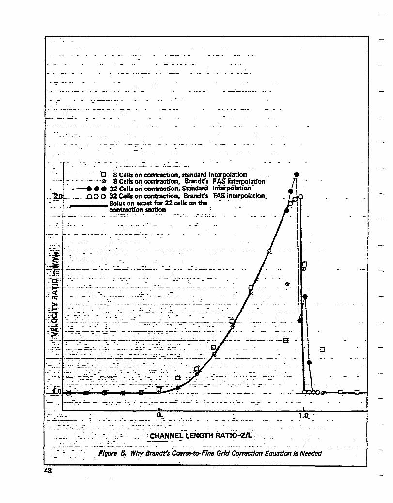
- -0 -S Cells on contraction. standard interpolation ---- --e- 8 Cells or.-contraction, Brandt's

_--I •••• 32 Cells on contraction, Standard _ ___ -'lO 0 32 Cells on contraction, Brandt's _--- Solution exact for 32 cells on the

contraetion section

-------- -----------,-

---, ----------- - - - - - ~ - --- ----_ ... --- .. ------,--- -----=:::---:- --:: .-- -=-- - .------ -

_ .. - r ... _ ..

F~lnterpolation interpolatloi..­FAS intarpalation _

--- - ... - -- - .. ---- - ------~--- ---- ..... ---- - ---- ... ... ...

-----:....:...-... ------ ----.--~:..:.. ----------- - ... -...... --- ---- ---- ==--=- ... .....:" ... - ---_ ... -~-= - --- ...:... -:: - -. -- - --- --- ...... - .. -.. --- -- -.;:.:----

-----~---------------- - ----- - --_ ... -... 0-__ .. __ ..... 0- .._ ------- ---------- - -- ----------..... - - - ... -- ...

1·- -.- .-.. -.. - ... - , ....

--- ---.. --.- --- --. ------ ......

~-.i.O~--I!__!!l--.. ~-i!t--ii"'---"""-:-

0.

----:..,;..:.:~~--- ..... -.-

• lJ I, ., I

I

If , , I \

\ , . \ Q

1 • \

--'-

--:_ Figure ~ Why Brandt's COfII'Seato-Fine Grid Co.rrection Equation i$ Needed

48

-- -

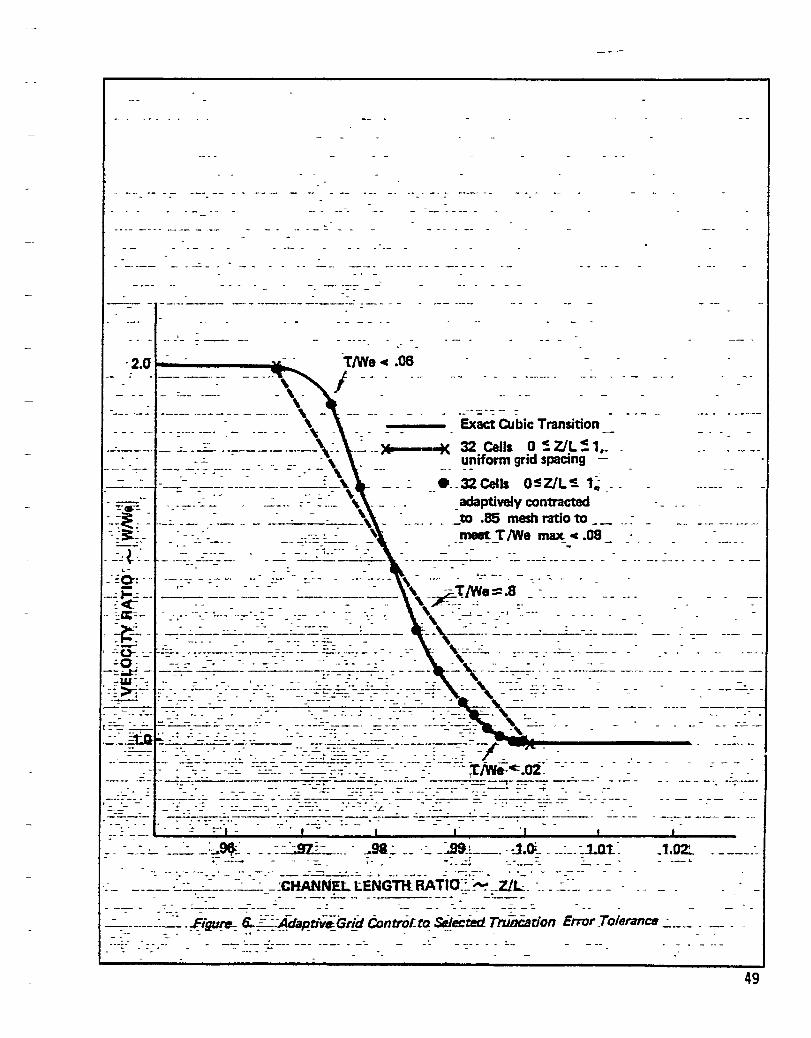
-2.0 t-----.... _. " - " -" ---- --- - -- - - ---- "

\ - - ---- ---. - -, - ----- --:-------\:-

-- \ ---. - -- ---- -: -- -- =- ----- " -- ---- ----- ----- --:-'---rat:-=-

--~- ---:~.: -

- --~----=g-:-- ----- - ---

"\ -------~:--\~-

..... --­,--

--= J-.;: -- --- ---- -- ----:<" =a;~-- -- - t --- --- -

~~ - ~-;:-----------:-~-:-~--:------

~&-~ --~~~-;~-~:-:-~ -~ ~~~:-~:- -.~~-~=~-~:-: w-­

':~ >-i-:-: . = ~ - ----:-:- -. -- -------:. _._-=-....-.-

~----.. -- - ~-_ .. -- ... ---

Exact Cubic Transition

32 Cells. 0 ~ ZJL ~ 1r uniform grid spacing -

• __ 32CeUs O~Z1L~ 1~

_ adaptively contracted _to .85 mesh ratio to __ _~3'lWa ~<.08_

-y-~-:- ---

---:. -- ... ----:. =--:--~~---:. - - --- -.:.....---.-- ~-- - - - - _-J..

-. -:-:-:::;----=-:-------~-------.-

__ = :.::!41.l ___ -___ - .A98 .:. _~L __ -:1.0i:. ___ : __ ~.1.Qt. ~ -=-~!

_____ ~::~---~~--~_-:CHANN~tENGm·RATIO~~~--Z1L- -____ ~~~ ___ _ -,-. -- - .-. --- ... - -- ----- -- - ---- -_ ...

_1.0%.

--=-=--______ -_~ _ -:figtJ!tl.~ 6..:~ ~#ap..ti~GrLi:J ContrOt.to. ~icied. TrriDCation Error _Toleran~ ~ ___ _ - .-- -:... - - -" - - -

49

End of Document