Comparison of real-time visualization of volumetric OCTdata sets by CPU-slicing and GPU-ray casting methods

Alfred R. Fullera, Robert J. Zawadzkib*, Bernd Hamanna and John S. Wernerb

aVisualization and Computer Graphics Research Group, Institute for Data Analysis andVisualization (IDAV), Department of Computer Science, UC Davis, One Shields Avenue,

Davis, CA 95616, USA;bVision Science and Advanced Retinal Imaging Laboratory (VSRI) and Department of

Ophthalmology & Vision Science, UC Davis, 4860 Y Street, Suite 2400, Sacramento, CA95817, USA;

ABSTRACT

We describe and compare two volume visualization methods for Optical Coherence Tomography (OCT) retinaldata sets. One of these methods is CPU-slicing, which is previously reported and used in our visualization engine.The other is GPU-ray casting. Several metrics including image quality, performance, hardware limitations andperception are used to grade the abilities of each method. We also discuss how to combine these methods tomake a scalable volume visualization system that supports advanced lighting and dynamic volumetric shadowingtechniques on a broad range of hardware. The feasibility of each visualization method for clinical application aswell as potential further improvements are discussed.

Keywords: Optical coherence tomography, imaging system, medical optics instrumentation, ophthalmology,volume visualization

1. INTRODUCTIONRecent progress in Fourier domain-Optical Coherence Tomography (Fd-OCT)1–5 has allowed for successful im-plementation for ophthalmic clinical applications.6–8 The fast acquisition speeds of Fd-OCT have led to thevolumetric imaging of in vivo retinal structures resulting in large volumetric data sets. Thus there is grow-ing demand for volume visualization and manipulation software. Following this direction over last three yearsour group has developed custom volume visualization software.9 This software has proven to be a powerfultool for conveying the information acquired using Optical Coherence Tomography (OCT) through computervisualization.

The goal of computer visualization is to convey meaningful information about a data set through a visualrepresentation. This is done by simulating stimuli on a computer screen that the human brain is accustomedto interpreting. However, computer visualization is limited by the resources of the computer generating thestimuli. This means that it can be costly in terms of computer processing power and resources to producephysically accurate stimuli akin to the natural world we experience and interpret every day. By dividing theperceptual experience into specific visual cues and targeting the specific perceptions associated with these cues,computer visualization has been able to find a middle ground between limited computer resources and the desiredconveyance of information. Naturally, as computers advance, this middle ground is continually being pushedforward to produce more meaningful visualizations.

Volume visualization of OCT retinal data sets strives to convey composition, shape, structure, and relativedepth and size of various retinal structures. The basic method behind volume visualization uses a transferfunction to convert the data values to visual stimuli. Visual stimuli are generated via color and opacity valueswhich are projected onto a computer screen to convey the basic composition of the data set. Additional visualcues are added to further enhance the user’s perception of the data set.

*rjzawadzki@ucdavis.edu; phone 1 916 734-5839; fax 1 916 734-4543; http://vsri.ucdavis.edu/

There are several significant visual cues that we consider for this particular application of volume visualization.A perspective projection of the visual stimuli enhances the user’s perception of both size and depth.10 Smoothlyanimated user-guided manipulation of the visualization allows the user to explore the composition of the dataset and enhances the perceived relative depth and size of different structures within the data set. Advancedlighting models enhance the perceived shape of these structures while shadows further enhance their relativedepth and size. Smooth animation and manipulation has been achieved with hardware-accelerated volumetricrendering and is widely used. Proper perspective is partially achieved with the current commonly used volumevisualization techniques while advanced lighting is rarely implemented and shadows are almost never used dueto the large cost associated with their computation.

We examine two volume visualization techniques that support these types of visual cues, CPU(central process-ing unit)-slicing and GPU(graphics processing unit)-ray casting. CPU-based methods are executed on the maincomputer’s processing unit which typically supports between one and four simultaneous operations. GPU-basedmethods are executed on the graphic card’s processing unit which can support anywhere from 16 to 512 (GeForce9800 GX2 SLI) simultaneous operations. CPU-Slicing was originally introduced by Cullip and Neumann11 andCabral et al.12 and has since been improved13–15 while the first single pass GPU-ray casting framework wasintroduced by Stegmaier et al.16

As is usually the case in computer visualization, the use of these techniques is primarily limited by theavailable computer resources. Lighting and shadows have generally been excluded from volume visualizations sothat smooth animation and manipulation can be archived given these limitations. However, we show that theseparticular visual cues can reasonably be implemented and combined into a single visualization on modern graphicshardware. Additionally, as both rendering methods have many implications with regard to their viability in aclinical setting, we describe a robust solution that utilizes both rendering methods to maximize the performanceand scalability of our overall system.

Section 2.1 describes the basic ideas behind CPU-slicing while Section 2.2 demonstrates how we can useGPU-ray casting to improve upon CPU-slicing when modern graphics hardware is available. However, GPU-ray casting also has another application. In Section 3.1 we describe a method that uses GPU-ray casting toimplement dynamic volumetric shadows. This implementation can be used with normal GPU-ray casting as wellas CPU-slicing. In Section 4.2 we discuss how these methods can be combined to scale to nearly any hardwareconfiguration. Section 4.3 extends upon this scalability to accommodate the needs of specific user activities.

2. RENDERING METHODS2.1 CPU-slicingBoth CPU-slicing and GPU-ray casting implement evenly spaced sampling volume reconstruction.17 However,the method by which the positions of these samples are calculated varies. CPU-slicing generates two-dimensionalslices of the volume perpendicular to the central view vector on the CPU and reconstructs the volume usingalpha blending on the GPU. Figure 1 shows a simplified two-dimensional representation of CPU-slicing. Theseslices are known as “proxy geometry,” as their only function is to trigger a program known as a “shader” torun on the GPU at the given position. The shader samples the volume and maps the data value to a colorand opacity (alpha value) through a transfer function like the one seen in Figure 2. As the user changes theorientation of the volume, the CPU must re-slice and re-render the entire volume. Figure 3 shows the samesimplified two-dimensional representation as Figure 1 except with the volume rotated.

As the sampling of the volume occurs on the graphics card, the GPU needs access to the volumetric data.However, graphics cards are limited by the amount of on-board memory available and OCT data sets tend toexceed this limit. To overcome this constraint, the volumetric data set is divided into data blocks of fixed size,which are rendered individually.18 Figure 3 shows a two-dimensional example of these data blocks. Each regionin Figure 3 must be sliced and rendered separately, greatly increasing the amount of work the CPU must performbefore the volume can be reconstructed on the GPU. Figure 4 show a small portion of the slices generated for areal OCT data set.

The basic equation that governs volumetric rendering is A(t, x) = 1 − e∫ t

0s(x+t′)dt′ where x is a position in

space, t is the spacing between adjacent samples and A is the opacity or alpha value accumulated from x to

Figure 1. A two-dimensional representation of the CPU-slicing algorithm. The CPU generates view-aligned polygons (orslices) at evenly spaced intervals throughout the bounding box of the volume. The graphics card projects these slices ontothe screen. For each screen pixel that is covered by a projected slice, the GPU runs a “shader” that samples the volumetricdata and returns an associated color and opacity. Alpha blending is used to aggregate theses colors and opacities for eachpixel.

Figure 2. An example of a transfer function from our application. A one-dimensional transfer function maps a data valueto a color and opacity for use in volumetric visualizations. The top region controls the opacity while the middle regioncontrols the color. The bottom region is used by the user to specify a color. A histogram of the data set is provided inthe background of the top region to guide the user in the selection of a meaningful transfer function.

(a) (b)Figure 3. (a) is the same volume as shown in Figure 1 except rotated and re-sliced. A volume must be re-sliced by theCPU for every change in orientation. (b) is this same rotated volume, but divided into separately rendered blocks. In thiscase, the volume must be re-sliced four times by the CPU for every change in orientation. The OCT data sets presentedin this paper contain about 160 of these blocks that need to be re-sliced for every change in orientation.

(a) (b)Figure 4. A small subset of the samples used in CPU-slicing to render a real OCT volumetric data set. Each color denotesthe location in the volumetric data set that is sampled through the relationship (x, y, z) = (red, green, blue). The samplesin (b) are from a volume divided into separately rendered data blocks. The coloring of the blocked volume shows thateach block is rendered with its own local data space coordinates.

Figure 5. Two pixels sampling two slices each from the CPU-slicing algorithm. The farther from the center of the screena pixel is, the less accurate our assumed constant t value becomes. Each dot represents a sample of the volumetric dataset and each line represents the path of samples for a single pixel.

x + t.19 In order to efficiently use this equation on the GPU we apply two approximations. First we set s(x)to be a constant between x to x + t. This eliminates the integral and A(t, x) = 1 − es(x)∗t. Then we set t tobe a constant which causes A to only be a function of x. With these simplifications we can accumulate colorcontributions from back to front with the recursive equation Ci = C(x) ∗ A(x) + (1 − A(x)) ∗ Ci−1 where Ci

is the color after accumulating the ith sample. To perform this operation we only need to convert a point inspace, x, into a color and opacity. This is done in a GPU shader by sampling the volume at point x and using auser-defined transfer function such as the one depicted in Figure 2 to convert the sampled value to a color andopacity. Unfortunately when we consider the samples used by CPU-slicing to reconstruct the volume we findthat a perspective projection of the slices does not maintain a constant t-value as exemplified in Figure 5. As aresult of this inaccuracy the volumetric rendering can appear faded on the periphery of the visualization. Thisfading scales with distance from the center of the image and sample spacing. One of the advantages of GPU-raycasting is that it does not suffer from this problem.

2.2 GPU-ray castingAs a replacement for CPU-slicing, GPU-ray casting uses the GPU to calculate a ray from the eye point to thevolume for each pixel and samples the volume along these rays. This is done by generating proxy geometry onthe front-facing boundary of the volume, which causes a GPU shader to execute along this boundary. Whilethe shader used in CPU-slicing is only responsible for sampling a single point in the data, the shader used inGPU-ray casting both samples all points needed by a given pixel and accumulates the values. These samplesare performed on a fixed interval of length t as seen in Figure 6. Figure 7 shows a small subset of the samplesused in GPU-ray casting for a real OCT data set both with and without blocking. These samples occur on thesurface of concentric spheres centered at the eye point with each adjacent sphere being exactly t apart. This is

Figure 6. Two rays from GPU-ray casting. These rays originate at the eye point and travel through different pixels onthe screen and into the volume. Each ray samples the volume on the same fixed interval, t. Each arrow represents a rayand each dot represents a sample of the volume.

(a) (b)Figure 7. A small subset of the samples used in GPU-ray casting to render a real OCT volumetric data set. Each colordenotes the location in the volumetric data set that is sampled through the relationship (x, y, z) = (red, green, blue). Thesamples in (b) are from a volume divided into separately rendered data blocks. Note that these samples occur on thesurface of concentric spheres instead of on parallel planes as seen in Figure 4.

distinctly different from CPU-slicing, where samples occur on parallel planes that are spaced t apart as seen inFigure 4. By maintaining a constant t-value, GPU-ray casting provides a better approximation to the volumerendering equation when using a perspective projection. Additionally, since no slicing is required, the CPU isonly tasked with specifying the boundary of the volume. However, since the shader used in GPU-ray casting isfar more complex than the one used in CPU-slicing, it requires a more capable graphics card.

GPU-ray casting allows for exact early ray termination. Since the shader used in GPU-ray casting is re-sponsible for all the samples along a single ray, it can detect when further samples will produce a negligiblecontribution to the final color accumulated along a ray. It can stop sampling the volume early and still returnan accurate result. Figure 8 shows the length along each ray that was sampled for the given volume.

3. VISUAL ENHANCEMENTS

3.1 Dynamic Volumetric ShadowsThe visibility function, v(x) is used to incorporate shadows into a lighting model. The visibility function, v(x),returns one to indicate full light and zero to indicate full darkness. Figure 9 shows this function on a real OCTdata set. Our application calculates this function directly for each sample by using the GPU to cast “shadowfeeler” rays towards the light source. The opacity of the volume is sampled along these rays and accumulated tofind the percentage of light that is not occluded. Figure 10 depicts this process. This method has traditionallybeen considered too slow to preserve interactivity of the application, but our application is able to overcome thiscomputational barrier by utilizing the GPU to cast these rays and implementing several methods to acceleratethe computation of these rays.

(a) (b)Figure 8. (a) is a normal GPU-ray casting rendering of an OCT data set while (b) shows the lengths of each ray usedto render the image in (a). In (b) shorter rays are dark while longer rays are light. Rays terminate at the front opaquesurface of the volume through the use of early ray termination. This approach can greatly reduce the number of samplesneeded to reconstruct the volume.

(a) (b)Figure 9. Rendering of the visibility function for both an unblocked (a) and a blocked (b) volume. The visibility function,v(x) is one in full light and zero in full darkness. The visibility function uses GPU-based “shadow feeler” rays to determinehow visible the light source is at a given point. These rays are restricted to the data in graphics memory, which explainswhy (b) shows discontinuities when occluding structures are in external data blocks.

Figure 10. Two rays from GPU-ray casting that also cast “shadow feeler” rays. These rays sample the volume to determinehow much light is visible at the given sample point. Casting these rays greatly increases the time it takes to render thevolume. However, this cost can be mitigated through the use of several optimizations of the ray casting algorithm. Eacharrow represents a ray and each dot represents a sample of the data set. The “shadow feeler” rays can also be cast whenusing CPU-slicing on certain hardware.

(a) (b)Figure 11. (a) shows the rays needed to calculate the visibility function at the given point when rendering separate datablocks. (b) shows the rays used when optimized shadow caching and early ray ternimation are applied for the same point.(b) also shows an additional point that requires no extra work to determine its visibility function. The ray in region 2 of(b) terminates early as its visibility function is zero before reaching the end of the data. Region 4 of (b) never needs tocast a shadow feeler ray as the value on the border between regions 2 and 4 already represents full darkness.

As with the normal GPU-ray casting, we can also use early ray-termination to speed up these shadow feelerrays. Additionally, the accuracy of the shadow feeler rays tends not to influence the visual fidelity of the resultingimage as much as rays used to reconstruct the volume. With this in mind we can increase the sample spacing, t,of the shadow feeler rays to something much larger than the t used to reconstruct the volume. Our applicationdefaults to a shadow sample spacing five times that of the normal sample spacing. We have also added theability to further increase this sample spacing dynamically on the GPU when sampling transparent regions ofthe volume.

This method fails when the data set is divided into blocks that are rendered separately. In this case, theshadow feeler ray cast at a given location only has access to a sub-region of the data. This causes problems whenthe location in question is shadowed by structures external to the available data. Figure 8 shows the resultingvisibility function of a blocked data set. To solve this problem our application uses a shadow cache. This cachestores intermediate values of the visibility function on the boundaries of blocked regions. This cache is madeavailable to the separate sub regions of the volume and restores the continuity of the visibility function. Eachshadow feeler ray is now actually divided into several different rays which are cast separately and accumulatedfor each sample point as seen in Figure 11. This approach has the added benefit of greatly reducing the amountof redundant sampling occurring and drastically limits the length of shadow feeler rays that are cast duringrendering. In the example presented in Figure 11(b), the points highlighted in region 4 never cast a shadowfeeler ray because the shadow cache already indicates full darkness. Figure 12 compares various volumes withand with out shadows.

3.2 Advanced LightingAny per-sample lighting model can be used to add lighting to both CPU-slicing and GPU-ray casting. There aremany different optical models19 that can be used. In our program, we have implemented one of the most popularlighting models, the Blinn-Phong model.20 This lighting model is ideal for volumes that contain well-definedsurfaces, as it is meant to approximate a micro-faceted surface and needs a normal vector at each sample point.These normals can be extracted by the GPU on the fly or pre-calculated and uploaded along with the volumedata. Since computing this normal on the fly introduces a large overhead and the normal values remain relativelyconstant, our application pre-calculates, smooths and down samples the normals. Figure 13 shows a rendering ofa pre-computed normal map. The calculation of these normals can be done on the CPU or more efficiently on theGPU. Technically these normals change when the opacity portion of the transfer function changes. However sincechanges in opacity usually only represent changes in the magnitude of the gradient vector, in most cases thesenormal vectors can be calculated once for each data set. The result of pre-calculating the normals, uploadingthem to graphics memory and using the Blinn-Phong lighting model on the GPU can be seen in Figure 14(b).Figure 14(c) shows a volume rendered with both Blinn-Phong lighting and shadows.

(a) (b)

(c) (d)Figure 12. A comparison of various volumes with and with out shadows. (b) and (d) are using GPU-based “shadow feeler”rays to cast shadows. (a) and (b) show a healthy retina while (c) and (d) illistrate retinal detachment.

Figure 13. The normal map extracted from the volume seen in Figure 8(a). It has been smoothed and down-sampled toimprove the visual quality and reduce its memory footprint. A normal map associates each voxel in the volumetric dataset to a normal vector. In this image, the normal vector (x, y, z) is represented by (red, green, blue).

(a) (b)

(c)Figure 14. Rendering of the photoreceptor layer of a retina suffering from macular degeneration. (a) has no lighting orshadows and is representative of the common form of volumetric visualization. (b) uses Blinn-Phong lighting model.(c) uses both Blinn-Phong lighting and shadows. In this case the size, shape and relative position of the drusen is noteasily perceived in (a) without rotating the volume. The visual cues added to (b) and (c) greatly increase the amount ofinformation that is conveyed to the viewer in a single image.

(a) (b)Figure 15. A comparison of CPU-slicing (a) and GPU-ray casting (b) when both use GPU-based “shadow feeler” raysto cast shadows. With small enough sample spacing, the visual difference is negligible but performance and hardwarerequirements of these methods differ.

4. PERFORMANCE SCALING4.1 ComparisonFigure 15 shows the same volume rendered both with CPU-slicing and GPU-ray casting. These images arenearly identical in appearance but differer in their performance and hardware requirements. The GPU-raycasting renders faster while the CPU-slicing is supported by a wider range of graphics cards. On the volume inFigure 15, which occupies 600x500 pixels and is reconstucted from a 997x350x97 data set scaled to 997x700x970,our application performs CPU-slicing in 100ms (10fps) and GPU-ray casting in 50ms (20fps) with a simple spacingof one sample per voxel and full lighting and shadows. From experience 100ms (10fps) - 66ms (15fps) is adequatefor interactive medical applications. On top of this there are many known algorithmic optimizations that wehave yet to implement in our system such as global empty space skipping and global early ray termination15

that can improve both CPU-slicing and GPU-ray casting.

4.2 Hardware LimitationsTable 1 provides an example of common hardware limitations and the available rendering methods associatedwith each configuration. Since our system can use both CPU-slicing and GPU-ray casting individually or incombination (CPU-slicing with GPU-shadows feeler rays) we can utilize the full resources of any system. Ourcurrent framework supports fixed function graphic processors as well as the latest graphic cards, thus we canvisualize volumetric data sets on relatively old laptops in addition to new high-end desktop computers.

Pixel Shader Min nVidia Generation Year Released CapabilitiesFixed Function < 3 Series <2001 CPU Slicing

GrayscaleSome TF

PS 2 3 Series 2001 Full TFPS 2.a 5 Series (FX) 2003 LightingPS 4 7 Series 2005 GPU Ray Casting or ShadowsPS 4+ 8 Series 2007 GPU Ray Casting and Shadows

Table 1. This table lists the minimum pixel shader version and nVidia chip generation required to use different capabilitiesof our system. Most desktops operating today will support at least PS 2.a while PS 4+ is only supported on high-endcomputers bought after 2006.

4.3 Useablility ScalingUsing the latest and most costly visualization technology is not always the best approach. This is the case withsome slower computers that support shadows, as rendering these shadows may increase the rendering time tosub-interactive levels. To address this issue, we have divided user-driven activities into six different categories and

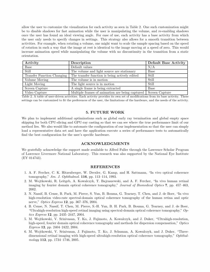
allow the user to customize the visualization for each activity as seen in Table 2. One such customization mightbe to disable shadows for fast animation while the user is manipulating the volume, and re-enabling shadowsonce the user has found an ideal viewing angle. For ease of use, each activity has a base activity from whichthe user only needs to specify changes in settings. This strategy also allows for a smooth transition betweenactivities. For example, when rotating a volume, one might want to scale the sample spacing based on the speedof rotation in such a way that the image at rest is identical to the image moving at a speed of zero. This wouldincrease animation speed while manipulating the volume with no discontinuity in the transition from a staticorientation.

Activity Description Default Base ActivityBase Default values N/AStill The volume and light source are stationary BaseTransfer Function Changing The transfer function is being actively edited StillVolume Moving The volume is in motion StillLight Moving The light source is in motion StillScreen Capture A single frame is being extracted BaseVideo Capture Multiple frames of animation are being captured Screen Capture

Table 2. A table of user-driven activities. Each activity provides its own set of modifications from its base activity. Thesesettings can be customized to fit the preferences of the user, the limitations of the hardware, and the needs of the activity.

5. FUTURE WORKWe plan to implement additional optimizations such as global early ray termination and global empty spaceskipping for both CPU-slicing and GPU-ray casting so that we can see where the true performance limit of ourmethod lies. We also would like to automate the configuration of our implementation so that the user can simplyload a representative data set and have the application execute a series of performance tests to automaticallyfind the best configuration for the user’s specific hardware.

ACKNOWLEDGMENTSWe gratefully acknowledge the support made available to Alfred Fuller through the Lawrence Scholar Programof Lawrence Livermore National Laboratory. This research was also supported by the National Eye Institute(EY 014743).

REFERENCES1. A. F. Fercher, C. K. Hitzenberger, W. Drexler, G. Kamp, and H. Sattmann, “In vivo optical coherence

tomography,” Am. J. Ophthalmol. 116, pp. 113–114, 1993.2. M. Wojtkowski, R. Leitgeb, A. Kowalczyk, T. Bajraszewski, and A. F. Fercher, “In vivo human retinal

imaging by fourier domain optical coherence tomography,” Journal of Biomedical Optics 7, pp. 457–463,2002.

3. N. Nassif, B. Cense, B. Park, M. Pierce, S. Yun, B. Bouma, G. Tearney, T. Chen, and J. de Boer, “In vivohigh-resolution video-rate spectral-domain optical coherence tomography of the human retina and opticnerve,” Optics Express 12, pp. 367–376, 2004.

4. B. Cense, N. Nassif, T. Chen, M. Pierce, S.-H. Yun, B. H. Park, B. Bouma, G. Tearney, and J. de Boer,“Ultrahigh-resolution high-speed retinal imaging using spectral-domain optical coherence tomography,” Op-tics Express 12, pp. 2435–2447, 2004.

5. M. Wojtkowski, V. Srinivasan, T. Ko, J. Fujimoto, A. Kowalczyk, and J. Duker, “Ultrahigh-resolution,high-speed, fourier domain optical coherence tomography and methods for dispersion compensation,” OpticsExpress 12, pp. 2404–2422, 2004.

6. M. Wojtkowski, V. Srinivasan, J. Fujimoto, T. Ko, J. Schuman, A. Kowalczyk, and J. Duker, “Three-dimensional retinal imaging with high-speed ultrahigh-resolution optical coherence tomography,” Ophthal-mology 112, pp. 1734–1746, 2005.

7. U. Schmidt-Erfurth, R. A. Leitgeb, S. Michels, B. Povazay, S. Sacu, B. Hermann, C. Ahlers, H. Sattmann,C. Scholda, A. F. Fercher, and W. Drexler, “Three-dimensional ultrahigh-resolution optical coherence to-mography of macular diseases,” Invest. Ophthalmol. Vis. Sci. 46, pp. 3393–3402, 2005.

8. S. Alam, R. J. Zawadzki, S. S. Choi, C. Gerth, S. S. Park, L. Morse, and J. S. Werner, “Clinical applicationof rapid serial fourier-domain optical coherence tomography for macular imaging,” Ophthalmology 113,pp. 1425–1431, 2006.

9. R. Zawadzki, A. Fuller, D. Wiley, B. Hamann, S. Choi, and J. Werner, “Adaptation of a support vectormachine algorithm for segmentation and visualization of retinal structures in volumetric optical coherencetomography data sets,” Journal of Biomedical Optics 12, pp. 041206 (1–8), 2007.

10. D. Vishwanath, A. Girschick, and M. Banks, “Why pictures look right when viewed from the wrong place,”Nature Neuroscience 8, pp. 1401–1410, 2005.

11. T. J. Cullip and U. Neumann, “Accelerating volume reconstruction with 3d texture hardware,” tech. rep.,Chapel Hill, NC, USA, 1994.

12. B. Cabral, N. Cam, and J. Foran, “Accelerated volume rendering and tomographic reconstruction usingtexture mapping hardware,” in VVS ’94: Proceedings of the 1994 symposium on Volume visualization,pp. 91–98, ACM Press, (New York, NY, USA), 1994.

13. R. Westermann and T. Ertl, “Efficiently using graphics hardware in volume rendering applications,” inSIGGRAPH ’98: Proceedings of the 25th annual conference on Computer graphics and interactive techniques,pp. 169–177, ACM Press, (New York, NY, USA), 1998.

14. C. Rezk-Salama, K. Engel, M. Bauer, G. Greiner, and T. Ertl, “Interactive volume on standard pc graphicshardware using multi-textures and multi-stage rasterization,” in HWWS ’00: Proceedings of the ACM SIG-GRAPH/EUROGRAPHICS workshop on Graphics hardware, pp. 109–118, ACM, (New York, NY, USA),2000.

15. W. Li, K. Mueller, and A. Kaufman, “Empty space skipping and occlusion clipping for texture-based volumerendering,” in VIS ’03: Proceedings of the 14th IEEE Visualization 2003 (VIS’03), IEEE Computer Society,(Washington, DC, USA), 2003.

16. S. Stegmaier, M. Strengert, T. Klein, and T. Ertl, “A simple and flexible volume rendering framework forgraphics-hardware-based raycasting,” in Volume Graphics, pp. 187–195, 2005.

17. J. T. Kajiya and B. P. VonHerzen, “Ray tracing volume densities,” SIGGRAPH Computer Graphics 18(3),pp. 165–174, 1984.

18. P. Bhaniramka and Y. Demange, “Opengl volumizer: a toolkit for high quality volume rendering of largedata sets,” in VVS ’02: Proceedings of the 2002 IEEE symposium on Volume visualization and graphics,pp. 45–54, IEEE Press, (Piscataway, NJ, USA), 2002.

19. N. Max, “Optical models for direct volume rendering,” IEEE Transactions on Visualization and ComputerGraphics 1(2), pp. 99–108, 1995.

20. J. F. Blinn, “Models of light reflection for computer synthesized pictures,” SIGGRAPH Computer Graph-ics 11(2), pp. 192–198, 1977.