C. Wohlin, M. Höst, P. Runeson and A. Wesslén, "Software Reliability", in Encyclopedia of Physical Sciences and Technology (third edition), Vol. 15,

Academic Press, 2001. 

Software Reliability

Claes Wohlin1, Martin Höst2, Per Runeson2 and Anders Wesslén2

1Blekinge Institute of Technology, Sweden2Lund University, Sweden

I. Reliability measurement and modeling: an introductionII. Usage-based testingIII. Data collectionIV. Software reliability modelingV. Experience packagingVI. Summary

GLOSSARY

Software reliability A software quality aspect that is measured in terms of mean time to failure or failure intensity of the software.

Software failure A dynamic problem with a piece of software.Software fault A defect in the software, which may cause a failure if being executed.Software error A mistake made by a human being resulting in a fault in the software.Software reliability estimation An assessment of the current value of the reliability

attribute. Software reliability prediction A forecast of the value of the reliability attribute at a

future stage or point of time.Software reliability certification To formally demonstrate system acceptability to

obtain authorization to use the system operationally. In terms of software reliability it means to evaluate whether the reliability requirement is met or not.

Software reliability is defined as “the probability for failure-free operation of a pro-gram for a specified time under a specified set of operating conditions”. It is one of the key attributes when discussing software quality. Software quality may be divided into quality aspects in many ways, but mostly software reliability is viewed as one of the key attributes of software quality.

The area of software reliability covers methods, models and metrics of how to estimate and predict software reliability. This includes models for both the operational profile, to capture the intended usage of the software, and models for the operational failure behavior. The latter type of models is then also used to predict the future behavior in terms of failures.

Before going deeper into the area of software reliability, it is necessary to define a set of terms. Already in the definition, the word failure occurs, which has to be defined and in particular differentiated from error and fault.

1

Failure is a dynamic description of a deviation from the expectation. In other words, a failure is a departure from the requirements of the externally visible results of program execution. Thus, the program has to be executed for a failure to occur. A fault is the source of a failure, statically residing in the program, which under certain conditions results in a failure. The term defect is often used as a synonym to fault. The fault in the software is caused by an error, where an error is a human action.

These definitions imply that the reliability depends not only on product attributes, such as number of faults, but also on how the product is used during operation, i. e. the oper-ational profile. This also implies that software reliability is different from software cor-rectness. Software correctness is a static attribute, i.e. number of faults, while reliability is a dynamic attribute, i.e. number of failures during execution.

The relations between the terms are summarized in Figure 1.

FIGURE 1. Relation between terms

Reliability is a probability quantity as stated in the definition. Probabilities are quanti-ties hard to capture and give adequate meanings for those whom are not used to them. It is often hard to interpret statements such as “the probability for a failure-free execu-tion of the software is 0.92 for a period of 10 CPU hours”. Thus, software reliability is often measured in terms of failure intensity and mean time to failure (MTTF), since they are more intuitive quantities for assessing the reliability. Then we state that “the failure intensity is 8 failures per 1 000 CPU hours” or “the MTTF is 125 CPU hours” which are quantities easier to interpret.

I. Reliability measurement and modeling: an introduction

A. Usage and reliability modeling

The reliability attribute is a complex one as indicated by the definitions above. The reliability depends on the number of remaining faults that can cause a failure and how these faults are exposed during execution. This implies two problems:

• The product has to be executed in order to enable measurement of the reliability. Furthermore the execution must be operational or resemble the conditions under which the software is operated. It is preferable if the reliability may be estimated before the software is put into operation.

• During execution, failures are detected and may be corrected. Generally, it is assumed that the faults causing the failures are removed.

causes

during execution

results in

during development

ReliabilityCorrectness

Error Fault Failure

2

In order to solve these problems, two different types of models have to be introduced:

• A usage specification. This specification, consisting of a usage model and a usage profile, specifies the intended software usage. The possible use of the system should be specified (usage model) and the usage quantities in terms of probabilities or fre-quencies (usage profile). Test cases to be run during software test are generated from the usage specification. The specification may be constructed based on data from real usage of similar systems or on application knowledge. If the reliability is measured during real operation, this specification is not needed. The usage-based testing is further discussed in Section II.

• A reliability model. The sequence of failures is modeled as a stochastic process. This model specifies the failure behavior process. The model parameters are deter-mined by fitting a curve to failure data. This implies also a need for an inference procedure to fit the curve to data. The reliability model can then be used to estimate or predict the reliability, see Section IV.

The principle flow of deriving a reliability estimate during testing is presented in Figure 2.

FIGURE 2. Reliability estimation from failure data

As mentioned above, failure intensity is an easier quantity to understand than reliabil-ity. Failure intensity can in most cases be derived from the reliability estimate, but often the failure intensity is used as the parameter in the reliability model.

As indicated by Figure 2, measurement of reliability involves a series of activities. The process related to software reliabililty consists of four major steps:

1. Create usage specificationThis step includes collecting information about the intended usage and creation of a usage specification.

2. Generate test cases and executeFrom the usage specification, test cases are generated and applied to the system under test.

3. Evaluate outcome and collect failure dataFor each test case, the outcome is evaluated to identify whether a failure occurred or not. Failure data is collected as required by the reliability model.

4. Calculate reliabilityThe inference procedure is applied on the failure data and the reliability model. Thus a reliability estimate is produced.

If the process is applied during testing, then process steps 2-4 are iterated until the soft-ware reliability requirement is met.

test cases failure data reliability estimate or prediction

UsageSpecification

SoftwareSystem

ReliabilityModel

3

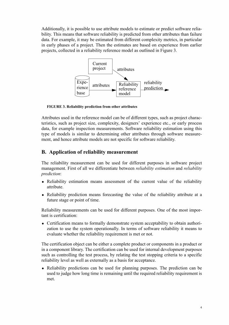
Additionally, it is possible to use attribute models to estimate or predict software relia-bility. This means that software reliability is predicted from other attributes than failure data. For example, it may be estimated from different complexity metrics, in particular in early phases of a project. Then the estimates are based on experience from earlier projects, collected in a reliability reference model as outlined in Figure 3.

FIGURE 3. Reliability prediction from other attributes

Attributes used in the reference model can be of different types, such as project charac-teristics, such as project size, complexity, designers’ experience etc., or early process data, for example inspection measurements. Software reliability estimation using this type of models is similar to determining other attributes through software measure-ment, and hence attribute models are not specific for software reliability.

B. Application of reliability measurement

The reliability measurement can be used for different purposes in software project management. First of all we differentiate between reliability estimation and reliability prediction:

• Reliability estimation means assessment of the current value of the reliability attribute.

• Reliability prediction means forecasting the value of the reliability attribute at a future stage or point of time.

Reliability measurements can be used for different purposes. One of the most impor-tant is certification:

• Certification means to formally demonstrate system acceptability to obtain authori-zation to use the system operationally. In terms of software reliability it means to evaluate whether the reliability requirement is met or not.

The certification object can be either a complete product or components in a product or in a component library. The certification can be used for internal development purposes such as controlling the test process, by relating the test stopping criteria to a specific reliability level as well as externally as a basis for acceptance.

• Reliability predictions can be used for planning purposes. The prediction can be used to judge how long time is remaining until the required reliability requirement is met.

attributes

attributes reliability prediction

Expe-rience base

Currentproject

Reliabilityreferencemodel

4

• Predictions and estimations can both be used for reliability allocation purposes. A reliability requirement can be allocated over different components of the system, which means that the reliability requirement is broken down and different require-ments are set on different system components.

Hence there are many areas for which reliability estimations and predictions are of great importance to control the software processes.

II. Usage-based testing

A. Purpose

Testing may be defined as any activity focusing on assessing an attribute of capability of a system or program, with the objective of determining whether it meets its required results. Another important aspect of testing is to make quality visible. Here, the attribute in focus is the reliability of the system and the purpose of the testing is to make the reliability visible. The reliability attribute is not directly measurable and must therefore be derived from other measurements. These other measurements must be col-lected during operation or during test that resembles the operation to be representative for the reliability.

The difficulty of the reliability attribute is that it only has a meaning if it is related to a specific user of the system. Different users experience different reliability, because they use the system in different ways. If we are to estimate, predict or certify the relia-bility, we must relate this to the usage of the system.

One way of relating the reliability to the usage is to apply usage-based testing. This type of testing is a statistical testing method and includes:

• a characterization of the intended use of the software, and the ability to sample test cases randomly from the usage environment.

• the ability to know whether the obtained outputs are right or wrong.

• a reliability model.

This approach has the benefits of validating the requirements and to accomplish this in a testing environment that is statistically representative of the real operational environ-ment.

Modeling the usage in a usage specification makes the characterization of the intended usage. This specification includes both how the users can use the system, i.e. the usage model, and the probabilities for different use, i.e. the usage profile. From the usage specification, test cases are generated according to the usage profile. If the profile has

5

the same distribution of probabilities as if the system is used during operation, we can get a reliability estimate that is related to the way the system is used, see Figure 4.

To evaluate whether the system responses from the system for a test case are right or wrong, an oracle is used. The oracle uses the requirements specification to determine the right responses. A failure is defined as a deviation of the system responses from its requirements. During the test, failure data is collected and used in the reliability model for the estimation, prediction or certification of the system’s reliability.

The generation of test cases and the decision whether the system responses are right or wrong, are not simple matters. The generation is done by “running through” the model and every decision is made as a random choice according to the profile. The matter of determining the correct system responses is to examine the sequence of user input and from the requirements determine what the responses should be.

B. Usage specifications overview

In order to specify the usage in usage-based testing, there is a need for a modeling technique. Several techniques have been proposed for the usage specification. In this section the most referred usage specification models are introduced.

Domain-based model. These models describe the usage in terms of inputs to the sys-tem. The inputs can be viewed as balls in an urn, where drawing balls from the urn gen-erates the usage. The proportion of balls corresponding to a specific input to the system is determined by the profile. The test cases are generated by repeatedly drawing balls from the urn, usually with replacement, see Figure 5.

FIGURE 4. Relationship between operation, usage specification and usage-based testing.

Operation

Usage

Represents

Sample

Usage-based testing

Modeling specification

Input x Input y

Input z

10% 45%

40%

Input a5%

FIGURE 5. The domain-based model.

6

The advantage of this model is that the inputs are assumed to be independent of each other. This is required for some types of reliability models.

The disadvantage is that the history of inputs is not captured and this model can only model the usage of batch-type system, where the inputs are treated as a separate run and the run is independent of other runs. The model is too simple to capture the com-plex usage of software systems. The input history has in most cases a large impact on the next input.

Algorithmic model. The algorithmic model is a refinement of the domain-based model. The refinement is that the algorithmic model takes the input history into account when selecting the next input. The model may be viewed as drawing balls from an urn, where the distribution of balls is changed by the input history.

To define the usage profile for the algorithmic model, the input history must be parti-tioned into a set of classes. For each class the distribution of the inputs is determined. If there are m classes and n different inputs, the usage profile is described in an m*nmatrix. The elements in the matrix are the probabilities for the different inputs given the input history class.

The advantages are that this model takes the input history into account when generat-ing the test cases and that it is easy to implement for automatic generation. The draw-back is that there is a need for the information, which is not in the usage profile, on how to change from one input history class to another, see Figure 6.

Operational profile. A way of characterizing the environment is to divide the execu-tion into a set of runs, where a run is the execution of a function in the system. If runs are identical repetitions of each other, these runs form a run type. Variations of a sys-tem function are captured in different run types. The specification of the environment using run types is called operational profile. The operational profile is a set of relative frequencies of occurrence of operations, where an operation is the set of run types asso-ciated with a system function. To simply the identification of the operational profile, a hierarchy of profiles is established, each making a refinement of the operational envi-ronment.

Input history 1

Input x Input y

Input z

10% 40%

50%

Input history 2

Input x Input y

Input z

25% 45%

30%Input history 3

Input x Input y

Input z

60% 5%

35%FIGURE 6. The algorithmic model.

7

The development of operational profiles is made in five steps:

• identify the customer profile, i.e. determine different types of customers, for exam-ple, private subscribers and companies (for a telephony exchange),

• define the user profile, i.e. determine if different types of users use the software in different ways, for example, subscribers and mainenance personnel,

• define the system modes, i.e. determine if the system may be operating in different modes,

• define the functional profile, i.e. determine the different functions of the different system modes, for example, different services available to a subscriber,

• define the operational profile, i.e. determine the probabilities for different opera-tions making up a function.

This hierarchy of profiles is used if there is a need of specifying more than one opera-tional profile. If there is only a need of specifying, for example, an average user, one operational profile is developed, see Figure 7.

Choosing operations according to the operational profile generates test cases.

The operational profile includes capabilities to handle large systems, but does not sup-port the detailed behavior of a user. It does not specify a strict external view, but takes some software internal structures into account. This is because the derivation of the operational profile needs information from the design or in some cases from the imple-mentation to make the testing more efficient.

Grammar model. The objective of the grammar model is to organize the descriptions of the software functions, inputs and the distributions of usage into a structural data-base from which test cases can be generated. The model has a defined grammar to describe the information of the database. The grammar defines how a test case looks like, in length, used functions, inputs and their distributions.

The grammar model is illustrated in Figure 8 with the example of selecting an item in a menu containing three items. A test case in the illustration is made up of a number of commands ending with a selection. A command is either up or down with equal proba-bility. First, the number of commands is determined. The number of commands is uni-formly distributed in the range of 0 to 1 with the probability 0.8 and in the range of 2 to

User Select menu

Function x

Function y

Normal use

System mode Z Item 1

Item 2

Item 3

10%

90%

25%

50%

25%

40%

30%

30%

FIGURE 7. The operational profile.

8

4 with the probability 0.2. The command is either “up” or “down” each with a proba-bility of 0.5. After the command, a selection is made and the test case is ended.

The outcome of a test case can be derived as the grammar gives both the initial soft-ware conditions and the inputs to it. The grammar is very easy to implement and test cases can be generated automatically. The drawback is that the grammar tends to be rather complex for a large system and which makes it hard to get an overview of how the system is used.

Markov model. The Markov model is an approach to usage modeling based on sto-chastic processes. The stochastic process that is used for this model is a Markov chain. The construction of the model is divided into two phases, the structural phase and the statistical phase.

During the structural phase the chain is constructed with its states and transitions. The transitions represent the input to the system and the state holds the necessary informa-tion about the input history. The structural model is illustrated in Figure 9, with the example of selecting an item in a menu containing three items.

FIGURE 8. The grammar model.

<test_case> ::= <no_commands> @ <command> <select>;

<no_commands> ::= ( <unif_int>(0,1) [prob(0.8)] | <unif_int>(2,4) [prob(0.2)]);

<command> ::= (<up> [prob(0.5)] | <down> [prob(0.5)]);

FIGURE 9. The Markov model.

Item 1

Item 2

Item 3

Up

Dow

n SelectShown

Hidden

Up

Up

Dow

nD

own

Select

Select

Invoke

Down

9

The statistical phase completes the Markov chain by assigning probabilities to the tran-sitions in the chain. The probabilities represent the expected usage in terms of relative frequencies. Test cases are then selected by “running through” the Markov model.

The benefits of Markov models are that the model is completely general and the gener-ated sequences look like a sample of the real usage as long as the model captures the operational behavior. Another benefit is that the model is based on a formal stochastic process, for which an analytical theory is available.

The drawback is that the number of states for a complex system tends to grow very large.

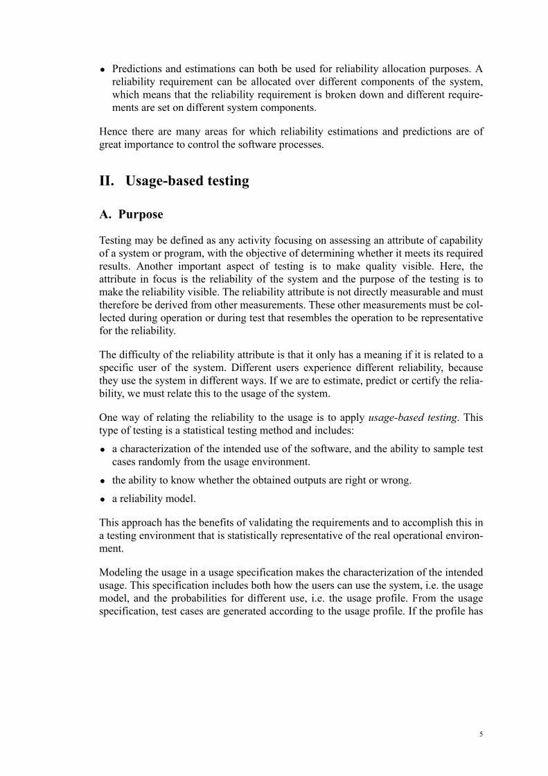
State hierarchy model. The state hierarchy (SHY) model was introduced to cope with modeling of complex systems with several user types and numerous different users. The objective of the model is to divide the usage-modeling problem into different lev-els, hence focusing on one aspect at the time. The number of levels in the model can easily be adapted to the needs when modeling, see Figure 10. The usage levels in the figure represent all usage of the system, the user type level represents users with the same structural usage and the usage subtype level represents all users with the same structural and statistical usage. The user level represents the users of the system and the service level describes which services a particular user can use. The structural descrip-tion of a service is described in the behavior level.

The hierarchy means that a service used by several users is only modeled once and then instantiated for all users using that particular service. The generation of test cases according to the anticipated software usage is made by “running through” the state hierarchy. The next event to be added to the test case is generated by first choosing a particular user type, then a user subtype, then a specific user of the chosen type and finally a service is chosen. Based on the state of the chosen service, a transition is made in the behavior level and an event is added to the test case.

Usage

Usertype

Usertype

User User User

Service Service Service Service

Usage level

User type level

User level

Service level

Behavior level

FIGURE 10. Illustration of the SHY model.

Sub-type

Sub-type

Sub-type

User

Service

User subtype level

10

The SHY model divides the usage profile into two parts, namely individual profile and hierarchical profile. The individual profile describes the usage for a single service, i.e. how a user behaves when using the available services. All users of a specific user type have the same individual profile. This profile refers to the transition probabilities on the behavior level.

The hierarchical profile is one of the major advantages with the SHY model as it allows for dynamic probabilities. It is obvious that it is more probable that a subscriber, connected to a telecommunication system, who has recently lifted the receiver, dials a digit, than that another user lifts the receiver. This means that the choice of a specific user to generate the next event depends on the actual state of the user and the states of its services. This is handled by introducing state weights which model the relative probability of generating the next event compared to the other states of the service. Thus, the state weights are introduced on the behavior level to capture that the proba-bility of the next event depends on the state in which the services of the different users are. The state weights are the basis for deriving the probabilities in the hierarchy.

One of the drawbacks of this model is that it is a complicated model and it can be hard to find a suitable hierarchy and to define the state weights. Another drawback is that since both services and users are dependent of each other, and the model tries to take this into account, the model becomes fairly complex although realistic.

Summary. The usage models presented here have their different advantages and disad-vantages. The choice of model depends on the application characteristics and how important the accuracy is.

If the system is a batch system then either the domain-based model or the algorithmic model is suitable, but not if the input history is important. If the input history is impor-tant, there are the grammar, Markov or the state hierarchy models. These models take the input history into account and the input can be described in detail if necessary. If the system is complex and has a large number of users the grammar model becomes very complex and the number of states in the Markov model grows very large. The models that can model the usage of these systems are the operational profile and the state hierarchy model. The operational profile is the most widely used model.

Before the testing can start, test cases must be generated from the usage specification. This can be done by “running through” the usage specification and logging test cases. Basically, transforming the usage specification into an executable representation gener-ates test cases and then it is executed with an oracle. The oracle determines the expected response from the system under the generated usage conditions. Another opportunity is that the oracle determines the correct output during testing, although this makes the testing less efficient in terms of calendar time.

C. Derivation of usage data

Reliability has only a meaning if it is related to the usage of the system. By applying usage-based testing, the system is tested as if being in operation and the failure data is representative of the operational failures. Usage-based testing includes a usage profile, which is a statistical characterization of the intended usage. The characterization is made in terms of a distribution of the inputs to the system during operation.

11

The usage profile is not easy to derive. When a system is developed it is either a com-pletely new system, or a redesign or modification of an existing system. If there is an older system, the usage profile can be derived from measuring the usage of the old sys-tem. On completely new systems there is nothing to measure and the derivation must be based on application knowledge and market analysis.

There are three ways to assign the probabilities in the usage profile.

Measuring the usage of an old system. The usage is measured during operation of an old system that the new system shall replace or modify. The statistics is collected, the new functions are analyzed and their usage is estimated based on the collected statis-tics.

Estimate the intended usage. When there are no old or similar systems to measure on, the usage profile must be estimated. Based on data from previous projects and on interviews with the end users an estimate on the intended usage is made. The end users can usually make a good profile in terms of relating the different function to each other. The function can be placed in different classes depending on how often a function is used. Each class is then related to the other by, for example, saying that one class is used twice as much as one other class. When all functions are assigned a relation, the profile is set according to these relations.

Uniform distribution. If there is no information available for estimating the usage profile, one can use a uniform distribution. This approach is sometimes called the unin-formed approach.

III. Data collection

A. Purpose

The data collection provides the basis for reliability estimations. Thus, a good data col-lection procedure is crucial to ensure that the reliability estimate is trustworthy. A pre-diction is never better than the data on which it is based. Thus it is important to ensure the quality of the data collection. Quality of data collection involves:

• collection consistency – data shall be collected and reported in the same way all the time, for example the time for failure occurrence has to be reported with enough accuracy.

• completeness – all data has to be collected, for example even failures for which the tester corrects the causing fault.

• measurement system consistency – the measurement system itself must as a whole be consistent, for example faults shall not be counted as failures, since they are dif-ferent attributes.

B. Measurement program

Measurement programs can be set up for a project, an organizational unit or a whole company. The cost is of course higher for a more ambitious program, but the gains are also higher the more experience is collected within a consistent measurement program.

12

Involving people in data collection implies, in particular, two aspects:

• Motivation – explain why the data shall be collected and for what purposes it is used.

• Feedback – report the measurements and analysis results back to the data providers.

Setting up a measurement program must be driven by specific goals. This is a means for finding and spreading the motivation as well as ensuring the consistency of the pro-gram, i.e., for example, that data is collected in the same way throughout a company. The Goal-Question-Metric (GQM) approach provides means for deriving goal-oriented measurements. Typical goals when measuring reliability are to achieve a certain level of reliability, to get measurable criteria for deciding when to stop testing or to identify software components, which contribute the most to reliability problems. The goals determine which data to collect for software reliability estimation and prediction.

C. Procedures

To achieve data of high quality, as much as possible shall be collected automatically. Automatic collection is consistent – not depending on human errors – and complete – as far as it is specified and implemented. However automatic collection is not generally applicable since some measurements include judgements, for example failure classifi-cation. Manual data collection is based on templates and forms, either on paper or elec-tronically.

D. Failure and test data

The main focus here is on software reliability models based on failure data. From the reliability perspective, failure data has to answer two questions:

• When did the failure occur?

• Which type of failure occurred?

The failure time can be measured in terms of calendar time, execution time or number of failures per time interval (calendar or execution). Different models require different time data. Generally it can be stated that using execution time increases the accuracy of the predictions, but requires a transformation into calendar time in order to be useful for some purposes. Planning of the test period is, for example, performed in terms of calendar time and not in execution time, thus there is a need for mapping between exe-cution time and calendar time. Keeping track of actual test time, instead of only meas-uring calendar time, can also be a means for improving the prediction accuracy.

When different failure severity categories are used, every failure has to be classified to fit into either of the categories. Reliability estimations can be performed for each cate-gory or for all failures. For example, it is possible to derive a reliability measure in gen-eral or for critical failures in particular.

13

IV. Software reliability modeling

A. Purpose

As stated in opening, software reliability can be defined as the probability of failure free operation of a computer program in a specified environment for a specified time. This definition is straightforward, but when the reliability is expressed in this way it is hard to interpret.

Some reasonable questions to ask concerning software reliability of software systems are:

• What is the level of reliability of a software system?

• How much more development effort must be spent to reach a certain reliability of a software system in a software development project?

• When to stop testing? That is, can we be convinced that the reliability objective is fulfilled, and how convinced are we?

Here the first question seems to be the easiest to answer. It is, however, not possible to directly measure the reliability of a system. This has to be derived as an indirect meas-ure from some directly measurable attributes of the software system. To derive the indirect measures of reliability from the directly measurable attributes, software relia-bility models are used. Examples of directly measurable attributes are the time between failures and the number of failures in a certain time period, (see Figure 11).

Directly measurableattributes Software

reliabilitymodel

Software reliability

FIGURE 11. The reliability can be derived from directly measurable attributes via a software reliability model.

14

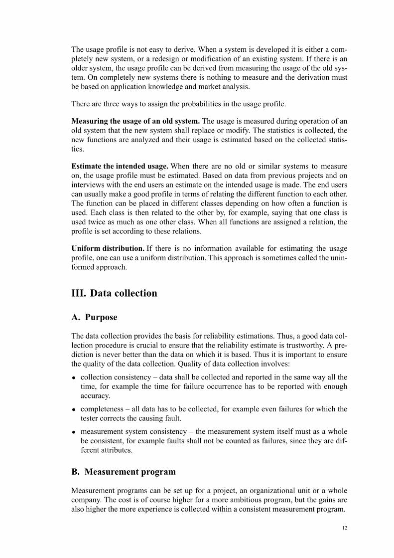
The main objective of a software reliability model is to provide an opportunity to esti-mate software reliability, which means that Figure 4 may be complemented as shown in Figure 12.

B. Definitions

As a starting point, we introduce some basic reliability theory definitions. Let X be a stochastic variable representing time to failure. Then the failure probability F(t) is defined as the probability that X is less than or equal to t. We also define the survival function as R(t) = 1 – F(t).

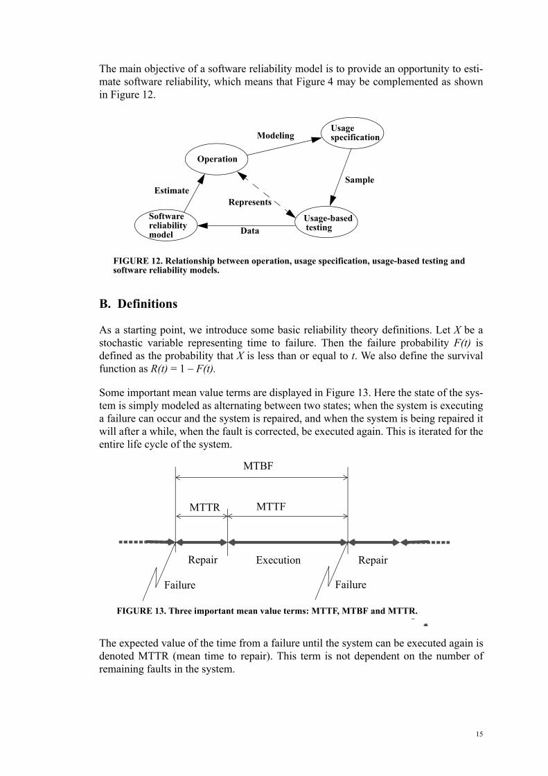
Some important mean value terms are displayed in Figure 13. Here the state of the sys-tem is simply modeled as alternating between two states; when the system is executing a failure can occur and the system is repaired, and when the system is being repaired it will after a while, when the fault is corrected, be executed again. This is iterated for the entire life cycle of the system.

The expected value of the time from a failure until the system can be executed again is denoted MTTR (mean time to repair). This term is not dependent on the number of remaining faults in the system.

FIGURE 12. Relationship between operation, usage specification, usage-based testing and software reliability models.

Operation

Usage

Represents

Sample

Usage-based testing

Modeling specification

Softwarereliabilitymodel Data

Estimate

Repair Execution Repair

MTBF

MTTFMTTR

Failure Failure

FIGURE 13. Three important mean value terms: MTTF, MTBF and MTTR.

15

The expected time from that the system is being executed after a repair activity until a new failure occurs is denoted MTTF1 (mean time to failure) and the most expected time between two consecutive failures is denoted MTBF (mean time between failures). The two last terms (MTTF and MTBF) are dependent on the remaining number of soft-ware faults in the system.

The above three terms are standard terms used in reliability theory in general. In hard-ware theory, however, the last two terms are often modeled as being independent of the age of the system. This can in most cases not be done for software systems.

Two simple but important relationships are

MTBF = MTTF + MTTR

Availability = MTTF / MTBF

When modeling software reliability, the repair times do not have any meaning. Instead only the times between consecutive failures are considered and therefore measured. In this case the only term of the above three that can be determined is the MTTF and the availability can not be determined.

C. Principles

As stated in the previous section the reliability must be derived as an indirect measure from directly measurable attributes of the software system. The directly measurable attributes are typically the times of failures, i.e. at what different times the different failures have occurred, or the number of failures in different time intervals.

These attributes can be measured in typically two different situations:

• When the software is under development and being tested: In this case, it is assumed that faults resulting in failures are corrected immediately. It could be the case that the faults are not removed immediately, but some time pass from that the failure is detected until the fault is located and corrected. Most software reliability models do, however, not account for this time.

• When the software is in use and is being maintained: In this case the faults are, in most cases, not corrected directly. This is instead done for the next release of the software system. In this case the MTBF and MTTF are constant between two con-secutive releases of the system.

The second situation is the simplest one and it is similar to basic hardware reliability theory. In this case the failure intensity can be modeled as constant for every release of the software. In the first case, however, the failure intensity can not be modeled as being constant. Here, it is a function of how many failures that have been removed. This is a major difference compared to basic hardware reliability theory where compo-nents are not improved every time they are replaced.

1. Sometimes the term is defined as the time from a randomly chosen time to the next failure.

16

The situation where the failure intensity is reduced for every fault that is corrected can be modeled in a number of different ways and a number of different models have been proposed. This section concentrates on the case when faults are directly corrected when their related failures occur.

The majority of all software reliability models are based on Markovian stochastic proc-esses. This means that the future behavior after a time, say t, is only dependent on the state of the process at time t and not on the history about how the state was reached. This assumption is a reasonable way to get a manageable model and it is made in many other engineering fields.

Regardless of the chosen model and data collection strategy, the model contains a number of parameters. These parameters must be estimated from the collected data. There are three different major estimation techniques for doing this:

• The maximum likelihood technique.

• The least square technique.

• The Bayesian technique.

The first two are the most used, while the last is more rarely used, because of its high level of complexity.

The application of reliability models is summarized in an example in Figure 14. In this example, the failure intensity is modeled with a reliability model. It could, however, be some other reliability attribute, such as mean time between failures. First the real val-ues of the times between failures in one realization are measured (1). Then the parame-ters of the model are estimated (2) with an inference method such as the maximum likelihood method. When this is done, the model can be used, for example, for predic-tion (3) of future behavior, see Figure 14.

D. Model overview

Reliability models can be classified into four different classes:

failureintensity

t

failureintensity

t

Reality

Model

failureintensity

t

failureintensity

tt

Parametersof model estimated

Model usedfor prediction

FIGURE 14. The application of reliability models. In this example the model is used for prediction.

1

2 3

17

• Time between failure models

• Failure count models

• Fault seeding models

• Input domain-based models

The first two classes are described in some more detail, while the latter two classes only are described briefly, since the two former classes of models are most common.

Time between failure models. Time between failure models concentrate on, as the name indicates, modeling the times between occurred failures. The first developed time between failure model was the Jelinski-Moranda model from 1972, where it is assumed that the times between failures are independently exponentially distributed. This means that, if Xi denotes the time between the (i-1):th and i:th failure, then proba-bility density function of Xi is defined as in equation 1.

Where is the failure intensity after the (i-1):th failure has occurred (and before the

i:th failure has occurred). In the Jelinski-Moranda model, is assumed to be a func-tion of the remaining number of failures and is derived as in equation 2.

Where N is the initial number of faults in the program and is a constant. The param-eters in the model can be interpreted as follows. Let N be the initial number of faults in the program and is a constant representing the per fault failure intensity.

The above formulas are together a model of the behavior of the software with respect to failures. It is not exactly representing the real behavior, merely a simplification of the real behavior. To be able to use this model, for example for prediction, N and must be estimated from the measured data. It is possible to make a maximum likeli-hood estimate of the parameters. The likelihood function that can be used to estimate N and is found in equation 3.

fXit( ) λie

λ– it= (1)

λi

λi

λi φ N i 1–( )–( )= (2)

φ

φ

φ

φ

L t1 …tn N φ,;,( ) fXiti( )

i 1=

n

∏ φ N i 1–( )–( )eφ N i 1–( )–( )– ti

i 1=

n

∏= = (3)

18

Where ti is the measured values of Xi, i.e. the measured times between failures, and n is the number of measured times. By taking the natural logarithm of the likelihood func-tion and simplifying we obtain equation 4.

This function should be maximized with respect to N and . To do this the first deriva-

tive with respect to N and can be taken. The and , which satisfy that both the derivatives equals 0, are the estimates we are looking for.

After the Jelinski-Moranda model was published a number of different variations of the model have been suggested. Examples are:

• Failures do not have to be corrected until a major failure has occurred.

• The failure intensity does not have to be constant between to successive failures. One proposal in the literature is to introduce an increasing failure rate (IFR) derived as , where t is the time elapsed since the last failure occurred.

• A variant of the Jelinski-Moranda model, which accounts for the probability of imperfect debugging, i.e. the probability that a fault is not removed in a repair activ-ity has been developed. With this model the failure intensity can be expressed as

, where p is the probability of imperfect debugging.

The Jelinski-Moranda model (with no variants) is presented here in some more detail, since it is an intuitive and illustrative model. In another situation when the main objec-tive is not to explain how to use reliability models, it may be appropriate to use one of the variants of the model, or a completely different model.

Failure count models. Failure count models are based on the number of failures that occur in different time intervals. The number of failures that occur is, with this type of model, modeled as a stochastic process, where N(t) denotes the number of failures that have occurred at time t.

Goel and Okomoto have proposed a failure count model where N(t) is described by a non-homogenous Poisson process. The fact that the Poisson process is non-homoge-nous means that the failure intensity is not constant, which means that the expected number of faults found at time t can not be described as a function linear in time (which is the case for an ordinary Poisson process). This is a reasonable assumption since the failure intensity decreases for every fault that is removed from the code. Goel and Oko-moto proposed that the expected number of faults found at time t could be described by equation 5.

Lln n φln N i– 1+( )lni 1=

n

∑ φ N i– 1+( )ti

i 1=

n

∑–+= (4)

φ

φ N̂ φ̂

λi φ N i 1–( )–( )t=

λi φ N p i 1–( )–( )=

m t( ) N 1 e bt––( )= (5)

19

Where N is the total number of faults in the program and b is a constant. The probabil-ity function for N(t) can be expressed as in equation 6.

The Goel and Okomoto model can be seen as the basic failure count model, and as with the Jelinski-Moranda model, a number of variants of the model have been proposed.

Fault seeding models. Fault seeding models are primarily used to estimate the total number of faults in the program. The basic idea is to introduce a number of representa-tive failures in the program, and let the testers find the failures that these faults result in. If the seeded faults are representative, i.e. they are equally failure prone as the ‘real’ faults, the number of real faults can be estimated by a simple reasoning.

If Ns faults have been seeded, Fs seeded faults have been found and Fr real faults have been found, then the total number of real faults can be estimated through equation 7.

A major problem with fault seeding models is to seed the code with representative faults. This problem is elegantly solved with a related type of models based on the cap-ture-recapture technique. With this type of model a number of testers are working inde-pendently and separately find a number of faults. Based on the number of testers that find each fault the number of faults in the code can be estimated. The more testers that find each fault, the larger share of the faults can be expected to be found, and the fewer testers that find each faults, the fewer of the total number of faults can be expected to be found.

Input domain-based models. By using this type of models, the input domain is divided into a set of equivalent classes, and then the software can be tested with a small number of test cases from each class. An example of an input domain-based model is the Nelson model.

E. Reliability demonstration

When the parameters of the reliability model have been estimated the reliability model can be used for prediction of the time to the next failure and the extra development time required until a certain objective is reached. The reliability of the software can be certified via interval estimations of the parameters of the model, i.e. confidence inter-vals are created for the model parameters. But often another approach, which is described in this section, is chosen.

A method for reliability certification is to demonstrate the reliability in a reliability demonstration chart. This method is based on that faults are not corrected when failures

P N t( ) n=( ) m t( )n

n!-------------e m t( )–= (6)

N NsFrFs-----⋅= (7)

20

are found, but if faults were corrected, this would only mean that the actual reliability is even better than what the certification says. This type of chart is shown in Figure 15.

To use this method, start in the origin of the diagram, and for each observed failure, draw a line to the right and one step up. The distance to the right is equal to the normal-ized time (time * failure intensity objective). For example, the objective may be that the mean time to failure should be 100 (failure intensity objective is equal to 1/100) and the measured time is 80, then the normalized time is 0.8. This means that when the normalized time is less than 1, in which case the plot comes closer to the reject line and on the other hand if it is larger than 1 then it comes closer to the accept line.

If the reached point has passed the accept line, the objective is met with the desired cer-tainty, but if the reject line is passed, it is with a desired certainty clear that the objec-tive is not met.

The functions for the two lines (accept line and reject line) are described by equation 8.

Where is the discrimination ratio (usually set to 2) and n is the number of observed failures. For the reject line A is determined by equation 9.

Normalized failure timeFa

ilure

num

ber

Accept

ContinueReject

FIGURE 15. Software reliability demonstration chart, which is based on sequential sampling.

Accept

line

Reject

line

n

x

x n( ) A n γln–1 γ–---------------------= (8)

γ

Arej1 β–

α------------ln= (9)

21

Where is the risk of saying that the objective is not met when it is and is the risk of saying that the objective is met when it is not. For the accept line A is determined by equation 10.

F. Accuracy of reliability predictions

The accuracy of the existing reliability models depends on the data that the prediction is based on. One model can get an accurate prediction for one set of test data, but can get an inaccurate prediction for another set of data. The problem is that it is impossible to tell which model that has an accurate prediction for a particular set of test data.

When predicting the future growth of the reliability, one method to evaluate the accu-racy of the model is to use a u-plot. A u-plot is used to determine if the predicted distri-bution function is on average close to the true distribution function. The distribution function for the time between failures is defined by equation 11.

The predicted distribution function is denoted . If Ti truly had the distribution

, then the random variable is uniformly distributed in (0,1). Let tibe the realization of Ti and calculate then ui is a realization of the random variable Ui. Calculating this for a sequence of predictions gives a sequence of {ui}. This sequence should look like a random sample from a uniform distribution. If there is a deviation from the uniform distribution, this indicates a difference between

and . The sequence of ui consists of n values. If the n ui’s are placed on the hori-zontal axis in a diagram and for each of these points a step function is increased with 1/(n+1), the result is a u-plot, see Figure 16. The u-plot is compared with the uniform dis-tribution, which is the line with unit slope through the origin. The distance between the unit line and the step function is then a measure of the accuracy of the predicted distri-bution function. In Figure 16, we see that predictions for short and long times are accu-

α β

Aaccβ

1 α–------------ln= (10)

FXit( ) P Xi t<( )≡ fXi

τ( )dτ

0

t

∫= (11)

F̂Xit( )

F̂Xit( ) Ui F̂Xi

Xi( )=

ui F̂Xixi( )=

F̂Xit( )

FXit( )

22

rate, but the predictions in between are a bit too optimistic, that is the plot is above the unit line.

V. Experience packaging

A. Purpose

In all measurement programs, collected experience is necessary to make full use of the potential in software product and process measurement and control. The experience base is a storage place for collected measurements, predictions and their interpreta-tions. Furthermore the models with parameters used are stored in the experience base.

The experience is used for different purposes:

• Constitute a baseline – reference values for the attributes to be measured and a long-term trend, for example, in an improvement program.

• Validate predictions – to judge whether predictions are reasonable by comparing data and predictions to the experience base.

• Improve predictions – the accuracy of predictions can be improved by using data from earlier projects.

• Enable earlier and more confident predictions – to predict, product and process attributes in the early phases, requires a solid experience base.

All these purposes are valid for measurement of product and process attributes in gen-eral and reliability in particular. In the reliability area, we focus on two types of models in the experience base:

• The usage model and profile applied in usage-based testing have to be stored with the predictions made since a reliability prediction always is based on a usage profile. There is also a reuse potential of the usage model and profile between different projects.

0 10

1

FIGURE 16. An example of a u-plot.

23

• The reliability model and its parameters are stored to constitute a basis for early pre-dictions of the reliability for forthcoming similar projects.

Experience packaging, related to these two model types, is further elaborated in Section B and Section C.

B. Usage model and profile

The usage model and profile are descriptions of the intended operational usage of the software. A reliability prediction is conducted based on test cases generated from a usage profile and is always related to that profile. A reliability prediction must hence always be stored in the experience base together with the usage profile used.

Comparing the prediction to the outcome in operational usage can validate a reliability prediction. If there is a considerable difference between predicted and experienced reli-ability, one of the causes may be discrepancies between the usage profile and the real operational profile. This has to be fed back, analyzed and stored as experience.

Continuous measurements on the operational usage of a product are the most essential experience for improving the usage profile. A reliability prediction derived in usage-based testing is never more accurate than the usage profile on which it is based.

The usage models and profiles as such contain a lot of information and represents val-ues invested in the derivation of the models and profiles. The models can be reused and thus utilizing the investments better. Different cases can be identified:

• Reliability prediction for a product in a new environment – the usage model can be reused and the usage profile is changed.

• Reliability prediction for an upgraded product – the usage model and profile can be reused but have to be extended and updated to capture the usage of added features of the product.

• Reliability prediction for a new product in a known domain – components of the usage model can be reused. Some usage model types support this better than others.

C. Reliability models

Experience related to the use of reliability models is just one type of experience that should be stored by an organization. Like other experiences, projects can be helped if experience concerning the reliability models is available.

In the first stages of testing, the estimations of the model parameters are very uncertain due to too few data points. Therefore it is very hard to estimate the values of the param-eters, and therefore experience would be valuable. If, for example, another project prior to the current project has developed a product similar to the currently developed product, then a good first value for the parameters would be to take the values of the prior project.

Another problem is to decide what model to choose for the project. As it was seen in the previous sections, a number of different reliability models are available and it is almost never obvious which one to choose. Therefore it could be beneficial to look at

24

previously conducted projects and compare these projects with the current one and also to evaluate the choice of models in previous projects. If similar projects have success-fully used one specific reliability model, then this reliability model could be a good choice for the current project, and on the other hand, if previously conducted similar projects have found a specific model to be problematic, this model should probably not be chosen.

Experience of reliability from previous projects can also be of use early in projects when reliability models can not yet be used, for example in the early planning phases. Experience can for example answer how much testing effort that will be required to meet a certain reliability objective.

Like with any other type of reuse, special actions must be taken to provide for later reuse. It is not possible to, when the experience is needed, just look into old projects and hope to find some the right information and conclusions from those old projects. Experience must have been collected systematically and stored in the previous projects. This means, for example, that:

• Measurements should be collected for the purpose of evaluation of the prediction models. Storing the choice of reliability model together with actual results can for example do this. This can be used to evaluate the reliability in for example a u-plot.

• Measurements should be collected for the purpose of understanding the model inde-pendent parameters such as initial time between failures and the fraction of found faults in different phases of the development.

The above mentioned measurements are just examples of measurements that can be collected to obtain experience. The intention is not to provide a complete set of meas-ures that should be collected with respect to reliability.

VI. Summary

When you use a software product, you want it to have as high quality as possible. But how do you define the quality of a software product? In the ISO standard 9126 the product quality is defined as: “the totality of features and characteristics of a software product that bear on its ability to satisfy stated or implied needs”. The focus here has been on one important quality aspect: the reliability of the software product.

Software reliability is a measure of how the software is capable of maintaining its level of performance under stated conditions for a stated period of time and is often expressed as a probability. To measure the reliability, the software has to be run under the stated conditions, which are the environment and the usage of the software.

As the reliability is related to the usage, it can not be measured directly. Instead it must be calculated from other measurements on the software. A measure often used is the failure occurrence, or more precisely the time between them, of the software which are related to the usage of the software.

To calculate the reliability from the failure data, the data must be collected during oper-ation or from testing that resembles operation. The testing method that is presented here is the usage-based testing method. In usage-based testing, the software is tested

25

with samples from the intended usage. These samples are generated from a characteri-zation of the intended usage and are representations of the operation. The characteriza-tion is made with a statistical model that describes how the software is used.

After the system is tested with usage-based testing, failure data that can be used for reliability calculations are available. The failure data are put into a statistical model to calculate the reliability. The calculations that are of interest are to estimate the current reliability, predict how the reliability will change or to certify with certain significance that the required reliability is achieved.

Software reliability is not only an important aspect for the end user, it can also be used for planning and controlling the development process. Reliability predictions can be used to judge how long time is remaining before the required reliability is obtained. Estimations or certifications can be used to certify if we have obtained the reliability requirement and as a criterion to stop testing.

26

BIBLIOGRAPHY

Fenton, N. and Pfleeger, S. L. (1996) Software Metrics: A Rigorous & Practical Approach. 2nd edition, International Thomson Computer Press.

Goel, A. and Okumoto, K. (1979) Time-dependent Error-Detection Rate Model for Software Reliability and Other Performance Measures, IEEE Transactions on Relia-bility, Vol. 28, No. 3, pp. 206-211.

Jelinski, Z. and Moranda, P. (1972), Software Reliability Research, Statistical Compu-ter Performance Evaluation, pp. 465-484.

Lyu, M. R. (editor) (1996) Handbook of Software Reliability Engineering. McGraw-Hill Book Company, New York, USA.

Musa, J. D. Iannino, A. and Okumoto, K. (1987) Software Reliability: Measurement, Prediction, Application. McGraw-Hill.

Musa, J. D. (1993) Operational Profiles in Software Reliability Engineering, IEEE Software, pp. 14-32, March 1993.

Musa, J. D. (1998) Software Reliability Engineering: More Reliable Software, Faster Development and Testing. McGraw-Hill.

van Solingen, R. and Berghout, E. (1999) The Goal/Question/Metric Method: A Practi-cal Guide for Quality Improvement and Software Development. McGraw-Hill Inter-national.

Xie, M. (1991) Software Reliability Modelling. World Scientific Publishing Co, Singa-pore, 1991.

27