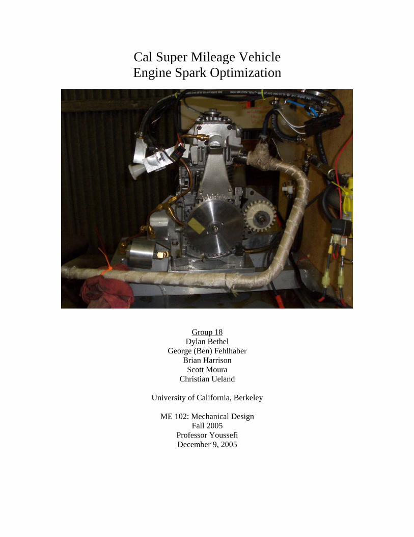
Cal Super Mileage Vehicle Engine Spark Optimization

Group 18 Dylan Bethel

George (Ben) Fehlhaber Brian Harrison Scott Moura

Christian Ueland

University of California, Berkeley

ME 102: Mechanical Design Fall 2005

Professor Youssefi December 9, 2005

1

Table of Contents Table of Contents..................................................................................................1 Background...........................................................................................................2 Mission Statement ................................................................................................2 Gantt Chart ...........................................................................................................3 Specifications & Requirements .............................................................................3 Conceptual Design................................................................................................4 Introduction to the Project .....................................................................................6

Electrical Components ......................................................................................7 Mechanical Components...................................................................................9

Drawings.............................................................................................................10 CAD.................................................................................................................10 Bill of Materials ................................................................................................11

Test Results ........................................................................................................12 Electronic Fuel Injection ..................................................................................12 PWM Speed Control........................................................................................14

Discussion ..........................................................................................................14 References .........................................................................................................15 Appendix.............................................................................................................16

Pictures ...........................................................................................................16

2

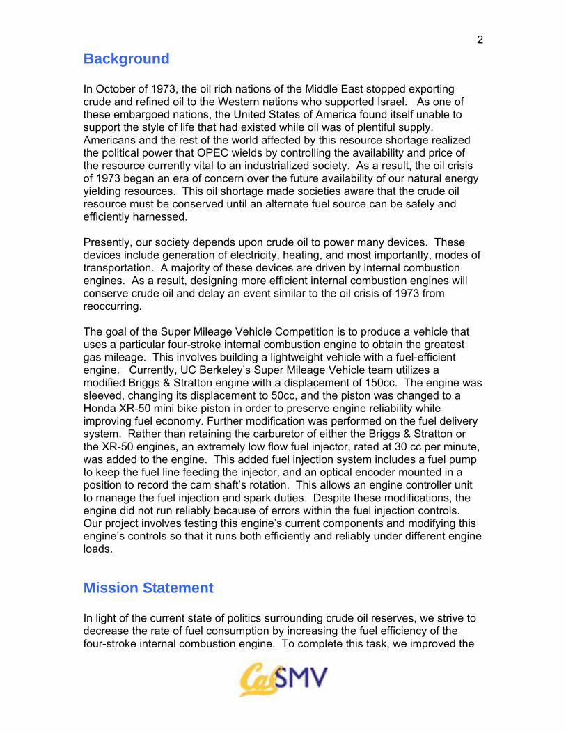
Background In October of 1973, the oil rich nations of the Middle East stopped exporting crude and refined oil to the Western nations who supported Israel. As one of these embargoed nations, the United States of America found itself unable to support the style of life that had existed while oil was of plentiful supply. Americans and the rest of the world affected by this resource shortage realized the political power that OPEC wields by controlling the availability and price of the resource currently vital to an industrialized society. As a result, the oil crisis of 1973 began an era of concern over the future availability of our natural energy yielding resources. This oil shortage made societies aware that the crude oil resource must be conserved until an alternate fuel source can be safely and efficiently harnessed.

Presently, our society depends upon crude oil to power many devices. These devices include generation of electricity, heating, and most importantly, modes of transportation. A majority of these devices are driven by internal combustion engines. As a result, designing more efficient internal combustion engines will conserve crude oil and delay an event similar to the oil crisis of 1973 from reoccurring.

The goal of the Super Mileage Vehicle Competition is to produce a vehicle that uses a particular four-stroke internal combustion engine to obtain the greatest gas mileage. This involves building a lightweight vehicle with a fuel-efficient engine. Currently, UC Berkeley’s Super Mileage Vehicle team utilizes a modified Briggs & Stratton engine with a displacement of 150cc. The engine was sleeved, changing its displacement to 50cc, and the piston was changed to a Honda XR-50 mini bike piston in order to preserve engine reliability while improving fuel economy. Further modification was performed on the fuel delivery system. Rather than retaining the carburetor of either the Briggs & Stratton or the XR-50 engines, an extremely low flow fuel injector, rated at 30 cc per minute, was added to the engine. This added fuel injection system includes a fuel pump to keep the fuel line feeding the injector, and an optical encoder mounted in a position to record the cam shaft’s rotation. This allows an engine controller unit to manage the fuel injection and spark duties. Despite these modifications, the engine did not run reliably because of errors within the fuel injection controls. Our project involves testing this engine’s current components and modifying this engine’s controls so that it runs both efficiently and reliably under different engine loads.

Mission Statement In light of the current state of politics surrounding crude oil reserves, we strive to decrease the rate of fuel consumption by increasing the fuel efficiency of the four-stroke internal combustion engine. To complete this task, we improved the

3efficiency of a modified Briggs & Stratton engine used by UC Berkeley’s Super Mileage Vehicle team. We optimized the spark time and injection time in the code that controls the fuel injection system. In doing so, the proper amount of power is generated with the least amount of fuel for all of the foreseeable engine loads. These loads were simulated by mechanically connecting the engine’s crankshaft to an alternator.

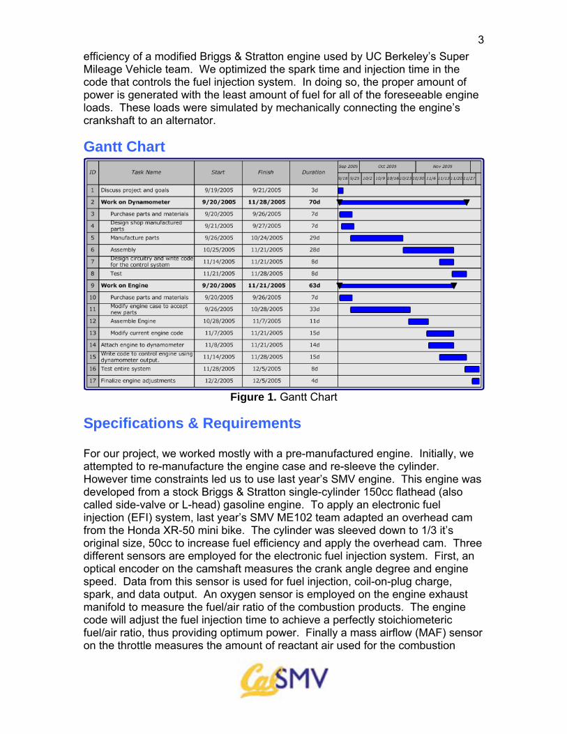
Gantt Chart

Figure 1. Gantt Chart

Specifications & Requirements For our project, we worked mostly with a pre-manufactured engine. Initially, we attempted to re-manufacture the engine case and re-sleeve the cylinder. However time constraints led us to use last year’s SMV engine. This engine was developed from a stock Briggs & Stratton single-cylinder 150cc flathead (also called side-valve or L-head) gasoline engine. To apply an electronic fuel injection (EFI) system, last year’s SMV ME102 team adapted an overhead cam from the Honda XR-50 mini bike. The cylinder was sleeved down to 1/3 it’s original size, 50cc to increase fuel efficiency and apply the overhead cam. Three different sensors are employed for the electronic fuel injection system. First, an optical encoder on the camshaft measures the crank angle degree and engine speed. Data from this sensor is used for fuel injection, coil-on-plug charge, spark, and data output. An oxygen sensor is employed on the engine exhaust manifold to measure the fuel/air ratio of the combustion products. The engine code will adjust the fuel injection time to achieve a perfectly stoichiometeric fuel/air ratio, thus providing optimum power. Finally a mass airflow (MAF) sensor on the throttle measures the amount of reactant air used for the combustion

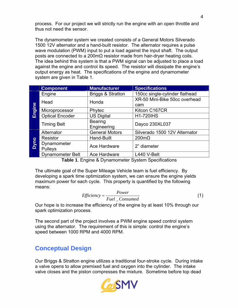
4process. For our project we will strictly run the engine with an open throttle and thus not need the sensor. The dynamometer system we created consists of a General Motors Silverado 1500 12V alternator and a hand-built resistor. The alternator requires a pulse wave modulation (PWM) input to put a load against the input shaft. The output posts are connected to a 200mΩ resistor made from hair-dryer heating coils. The idea behind this system is that a PWM signal can be adjusted to place a load against the engine and control its speed. The resistor will dissipate the engine’s output energy as heat. The specifications of the engine and dynamometer system are given in Table 1.

Component Manufacturer Specifications Engine Briggs & Stratton 150cc single-cylinder flathead

Head Honda XR-50 Mini-Bike 50cc overhead cam

Microprocessor Phytec Kitcon C167CR Optical Encoder US Digital H1-720IHS En

gine

Timing Belt Bearing Engineering Dayco 230XL037

Alternator General Motors Silverado 1500 12V Alternator Resistor Hand-Built 200mΩ Dynamometer Pulleys Ace Hardware 2” diameter D

yno

Dynamometer Belt Ace Hardware L440 V-Belt Table 1. Engine & Dynamometer System Specifications

The ultimate goal of the Super Mileage Vehicle team is fuel efficiency. By developing a spark time optimization system, we can ensure the engine yields maximum power for each cycle. This property is quantified by the following means:

Consumed_FuelPowerEfficiency = (1)

Our hope is to increase the efficiency of the engine by at least 10% through our spark optimization process. The second part of the project involves a PWM engine speed control system using the alternator. The requirement of this is simple: control the engine’s speed between 1000 RPM and 4000 RPM.

Conceptual Design Our Briggs & Stratton engine utilizes a traditional four-stroke cycle. During intake a valve opens to allow premixed fuel and oxygen into the cylinder. The intake valve closes and the piston compresses the mixture. Sometime before top dead

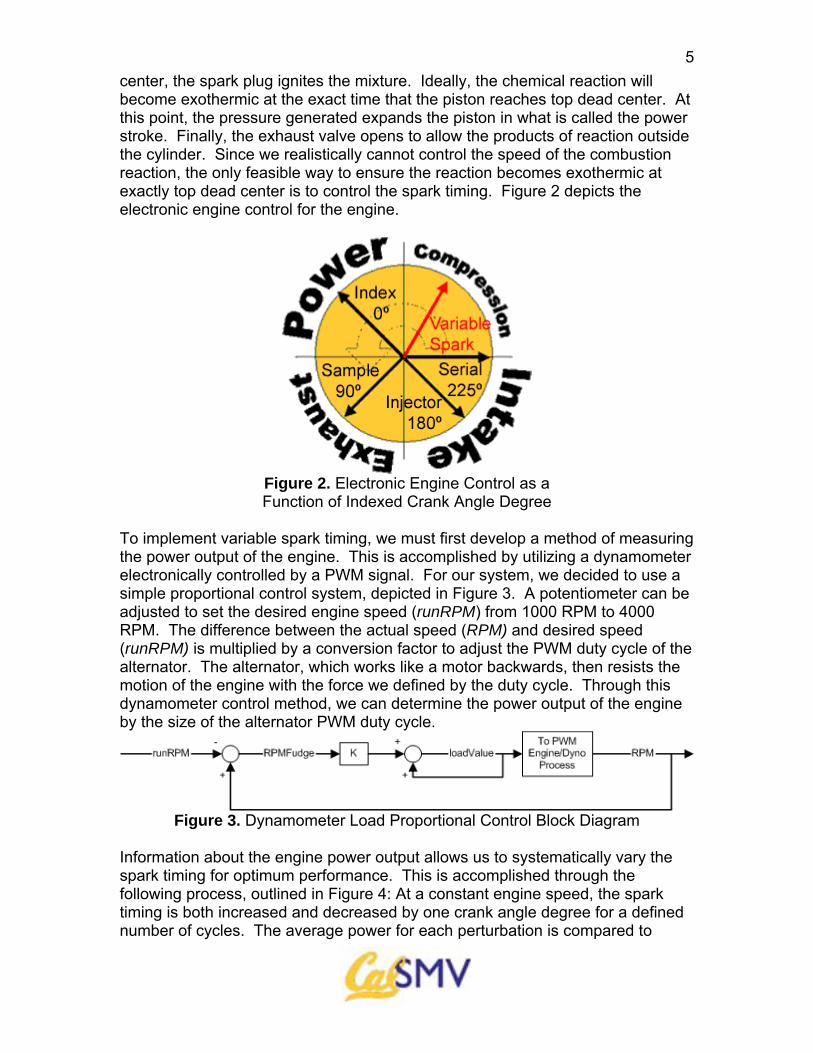
5center, the spark plug ignites the mixture. Ideally, the chemical reaction will become exothermic at the exact time that the piston reaches top dead center. At this point, the pressure generated expands the piston in what is called the power stroke. Finally, the exhaust valve opens to allow the products of reaction outside the cylinder. Since we realistically cannot control the speed of the combustion reaction, the only feasible way to ensure the reaction becomes exothermic at exactly top dead center is to control the spark timing. Figure 2 depicts the electronic engine control for the engine.

Figure 2. Electronic Engine Control as a Function of Indexed Crank Angle Degree

To implement variable spark timing, we must first develop a method of measuring the power output of the engine. This is accomplished by utilizing a dynamometer electronically controlled by a PWM signal. For our system, we decided to use a simple proportional control system, depicted in Figure 3. A potentiometer can be adjusted to set the desired engine speed (runRPM) from 1000 RPM to 4000 RPM. The difference between the actual speed (RPM) and desired speed (runRPM) is multiplied by a conversion factor to adjust the PWM duty cycle of the alternator. The alternator, which works like a motor backwards, then resists the motion of the engine with the force we defined by the duty cycle. Through this dynamometer control method, we can determine the power output of the engine by the size of the alternator PWM duty cycle.

Figure 3. Dynamometer Load Proportional Control Block Diagram

Information about the engine power output allows us to systematically vary the spark timing for optimum performance. This is accomplished through the following process, outlined in Figure 4: At a constant engine speed, the spark timing is both increased and decreased by one crank angle degree for a defined number of cycles. The average power for each perturbation is compared to

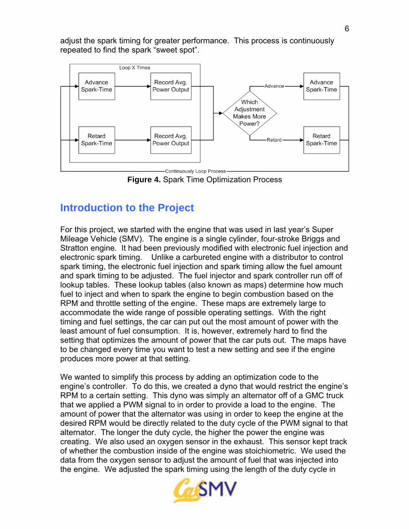
6adjust the spark timing for greater performance. This process is continuously repeated to find the spark “sweet spot”.

Figure 4. Spark Time Optimization Process

Introduction to the Project For this project, we started with the engine that was used in last year’s Super Mileage Vehicle (SMV). The engine is a single cylinder, four-stroke Briggs and Stratton engine. It had been previously modified with electronic fuel injection and electronic spark timing. Unlike a carbureted engine with a distributor to control spark timing, the electronic fuel injection and spark timing allow the fuel amount and spark timing to be adjusted. The fuel injector and spark controller run off of lookup tables. These lookup tables (also known as maps) determine how much fuel to inject and when to spark the engine to begin combustion based on the RPM and throttle setting of the engine. These maps are extremely large to accommodate the wide range of possible operating settings. With the right timing and fuel settings, the car can put out the most amount of power with the least amount of fuel consumption. It is, however, extremely hard to find the setting that optimizes the amount of power that the car puts out. The maps have to be changed every time you want to test a new setting and see if the engine produces more power at that setting. We wanted to simplify this process by adding an optimization code to the engine’s controller. To do this, we created a dyno that would restrict the engine’s RPM to a certain setting. This dyno was simply an alternator off of a GMC truck that we applied a PWM signal to in order to provide a load to the engine. The amount of power that the alternator was using in order to keep the engine at the desired RPM would be directly related to the duty cycle of the PWM signal to that alternator. The longer the duty cycle, the higher the power the engine was creating. We also used an oxygen sensor in the exhaust. This sensor kept track of whether the combustion inside of the engine was stoichiometric. We used the data from the oxygen sensor to adjust the amount of fuel that was injected into the engine. We adjusted the spark timing using the length of the duty cycle in

7order to find the setting that created the most amount of power. We also added some optimization code to the engine’s controller. This optimization code adjusts the fuel injection and spark timing in order to find the best settings that allow the engine to create the most amount of power.

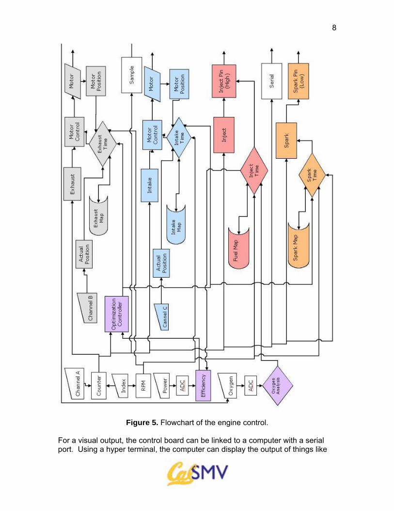
Electrical Components We started with the control board that was previously used with the engine. We used this board so that most of the code for the engine was already written, all we had to do was to add our optimization portion to it. There were three pots connected to this control board. One of the pots adjusted the RPM setting that we wanted to keep the engine at once we turned on the load. The other two controlled the initial fuel injection and spark timing in order to get the engine running. Once running, the engine’s optimization code would change that fuel amount and spark timing in order to optimize the engine’s performance. There are also kill switches for the fuel injector, spark ignition, and alternator load. This allowed us to kill the engine quickly in case there were any unforeseen problems. The control board communicated with the fuel injector and spark regulator, and controlled the load that the alternator applied. In order to control the load that the alternator was applied to the engine, the control board output a PWM signal. This signal was run through a Schmitt Trigger in order to act as an output buffer. After the Schmitt Trigger, the signal was run through an H-bridge that was powered at 12 volts. This H-bridge transformed the PWM signal that the control board output into a signal that could be inputted into the alternator. The input of the alternator was connected to this H-bridge, and that’s how the load to the engine was controlled. The output of the alternator was connected to a handmade resistor that had an extremely low resistance. This simply acted as a way to dissipate the excess energy through heat. The resistor created by placing heating coils from a hair dryer into a parallel setup. These wires will heat up and dissipate the excess energy from the alternator. There was also an optical encoder attached to the end of the camshaft. This communicated with the control board in the same way that the fuel injector and spark regulator did. The optical encoder kept track of a couple of things. First of all, it gave us the RPM of the engine. This was compared to our desired RPM and then the duty cycle was adjusted accordingly. The optical encoder also told us at what position the spark fired. Since we already knew where top dead center was, the recording the position when the spark ignites told us how far the spark was advanced before top dead center. Finally, the optical encoder acted as a counter and a trigger. It would keep track of when to inject the fuel, ignite the spark, and take the data to be used in the optimization code. A flow diagram for how all of the electrical components worked together can be seen in Figure 5.

8

Figure 5. Flowchart of the engine control. For a visual output, the control board can be linked to a computer with a serial port. Using a hyper terminal, the computer can display the output of things like

9the RPM, actual and desired, and the difference between the two, spark timing before top dead center, and oxygen sensor readings.

Mechanical Components The only mechanical components of our project were the engine and the dyno. The engine was a single cylinder, four-stroke Briggs and Stratton engine that had been modified. It has a mechanical oil pump that is driven by the timing belt on the crank and camshaft. The fuel pump is electrical though, driven by a 12V power source. The engine uses a single overhead camshaft to operate the intake and exhaust valves. An electric starter turns the flywheel in order to turn the engine over when starting it. The engine runs on isooctane fuel. The engine is connected to the dyno by a pulley system that is connected to the crankshaft. The pulley system drives the dyno, which is just an alternator off of a GMC truck. The shaft of the alternator was not long enough to accommodate the pulley system to drive it, so we had to make an extension for the shaft. Normally, when the alternator is turned, it changes mechanical power into electrical power. For our purposes, we’ve reversed that. The alternator is supplied an electrical power in the form of a PWM signal. It then converts that electrical power into a mechanical load, which restricts the RPM of the engine to our desired settings.

10

Drawings

CAD

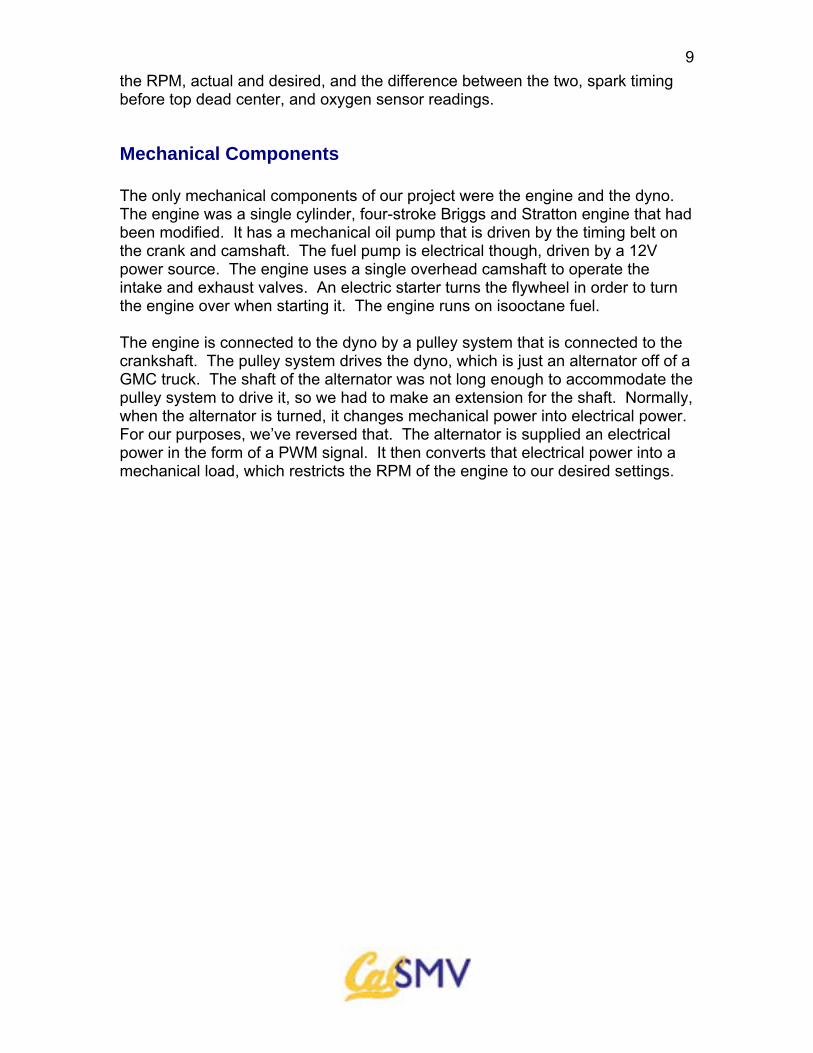
Figure 6. SMV Engine Assembly

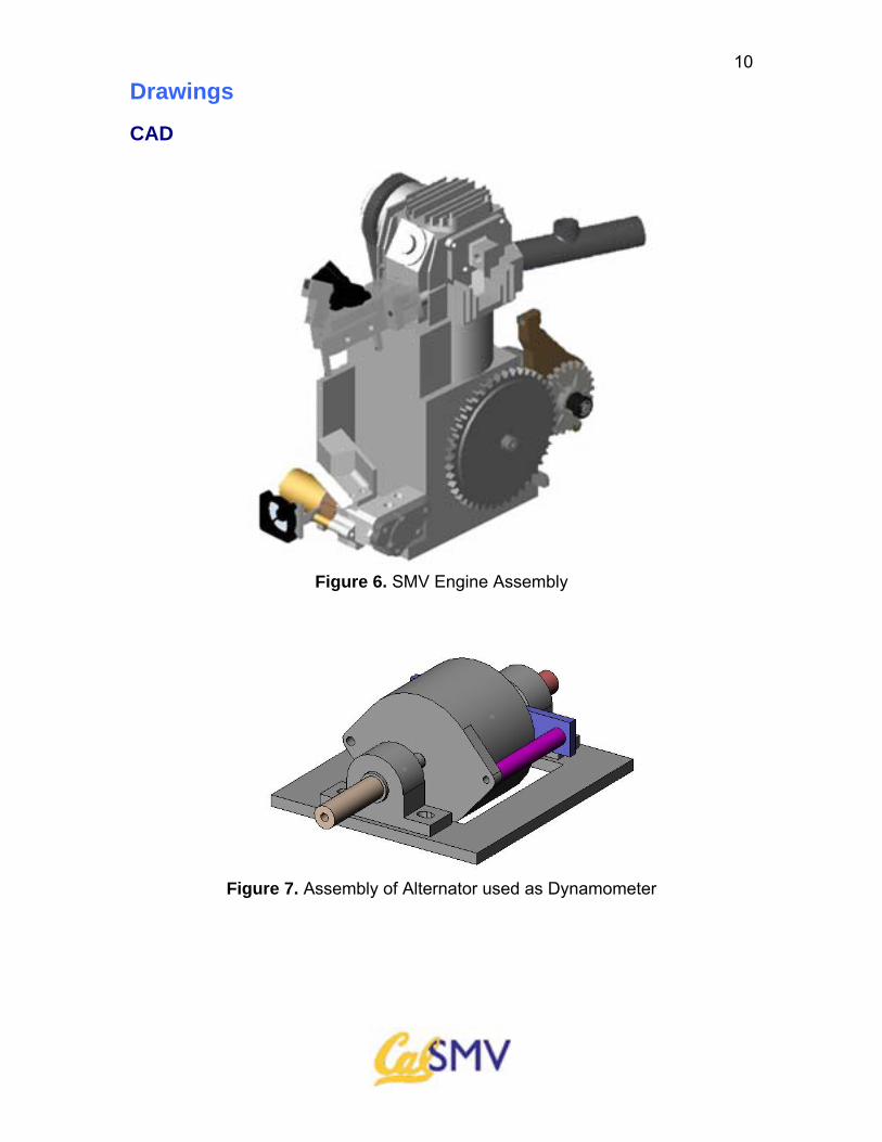
Figure 7. Assembly of Alternator used as Dynamometer

11

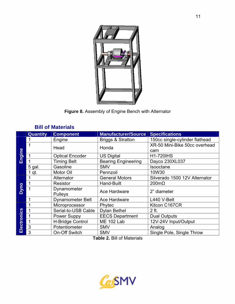
Figure 8. Assembly of Engine Bench with Alternator

Bill of Materials Quantity Component Manufacturer/Source Specifications

1 Engine Briggs & Stratton 150cc single-cylinder flathead 1 Head Honda XR-50 Mini-Bike 50cc overhead

cam 1 Optical Encoder US Digital H1-720IHS 1 Timing Belt Bearing Engineering Dayco 230XL037 5 gal. Gasoline SMV Isooctane

Engi

ne

1 qt. Motor Oil Pennzoil 10W30 1 Alternator General Motors Silverado 1500 12V Alternator 1 Resistor Hand-Built 200mΩ 1 Dynamometer

Pulleys Ace Hardware 2” diameter Dyn

o

1 Dynamometer Belt Ace Hardware L440 V-Belt 1 Microprocessor Phytec Kitcon C167CR 1 Serial-to-USB Cable Dylan Bethel 2 ft. 1 Power Suppy EECS Department Dual Outputs 1 H-Bridge Control ME 102 Lab 12V-24V Input/Output 3 Potentiometer SMV Analog

Elec

tron

ics

3 On-Off Switch SMV Single Pole, Single Throw Table 2. Bill of Materials

12

Test Results

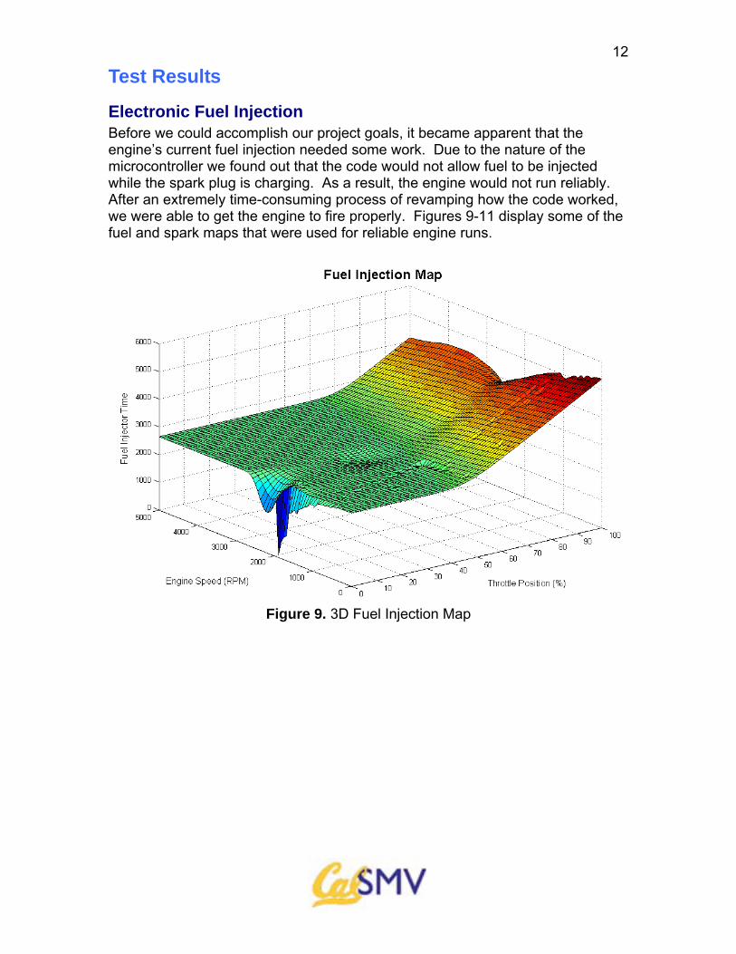
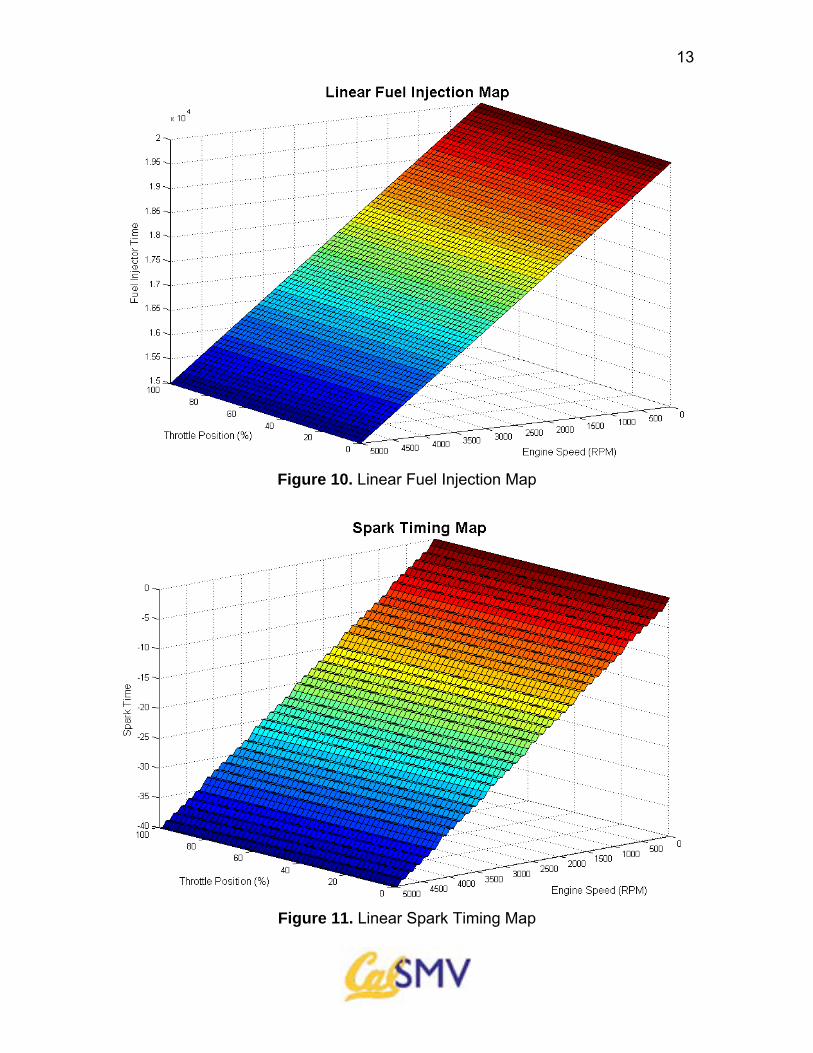
Electronic Fuel Injection Before we could accomplish our project goals, it became apparent that the engine’s current fuel injection needed some work. Due to the nature of the microcontroller we found out that the code would not allow fuel to be injected while the spark plug is charging. As a result, the engine would not run reliably. After an extremely time-consuming process of revamping how the code worked, we were able to get the engine to fire properly. Figures 9-11 display some of the fuel and spark maps that were used for reliable engine runs.

Figure 9. 3D Fuel Injection Map

13

Figure 10. Linear Fuel Injection Map

Figure 11. Linear Spark Timing Map

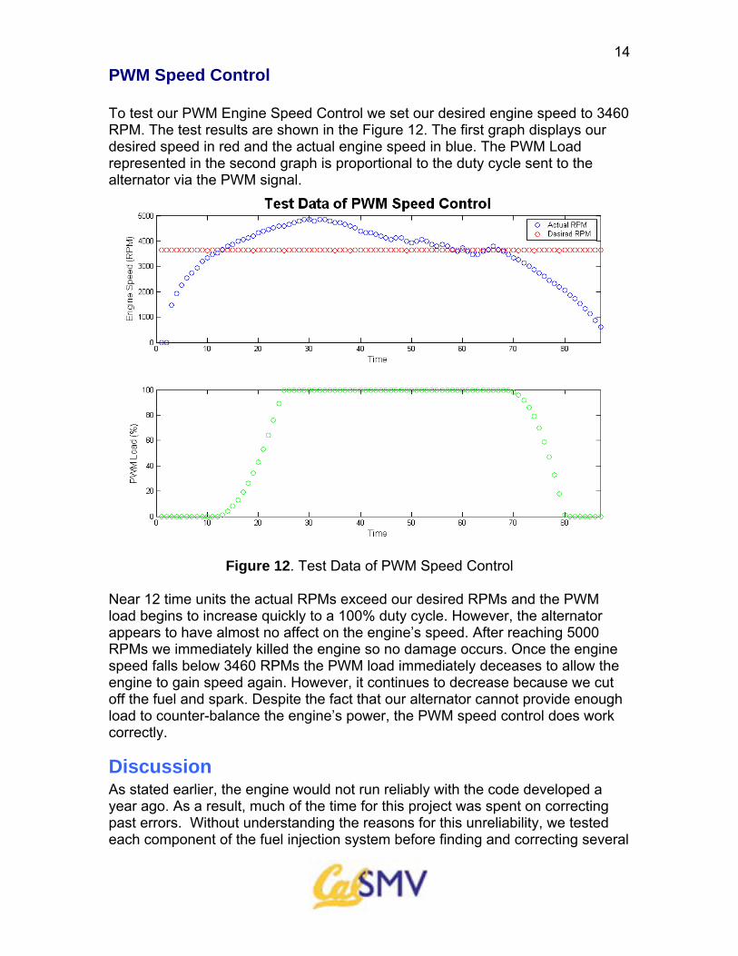
14PWM Speed Control To test our PWM Engine Speed Control we set our desired engine speed to 3460 RPM. The test results are shown in the Figure 12. The first graph displays our desired speed in red and the actual engine speed in blue. The PWM Load represented in the second graph is proportional to the duty cycle sent to the alternator via the PWM signal.

Figure 12. Test Data of PWM Speed Control

Near 12 time units the actual RPMs exceed our desired RPMs and the PWM load begins to increase quickly to a 100% duty cycle. However, the alternator appears to have almost no affect on the engine’s speed. After reaching 5000 RPMs we immediately killed the engine so no damage occurs. Once the engine speed falls below 3460 RPMs the PWM load immediately deceases to allow the engine to gain speed again. However, it continues to decrease because we cut off the fuel and spark. Despite the fact that our alternator cannot provide enough load to counter-balance the engine’s power, the PWM speed control does work correctly.

Discussion As stated earlier, the engine would not run reliably with the code developed a year ago. As a result, much of the time for this project was spent on correcting past errors. Without understanding the reasons for this unreliability, we tested each component of the fuel injection system before finding and correcting several

15errors. The first problematic component that we tested was the fuel injector. We found that the injector could inject while it was powered but not while the engine was running. With this observation, we deduced that errors existed within the code controlling the fuel injection system. As a result, we rewrote much of the code to debug it and perform newly needed tasks. We observed that the code was commanding the microcontroller to begin injection while the spark plug was charging. Because the microcontroller cannot perform two tasks simultaneously, the engine would not run. To solve this problem, we altered the way that the spark plug was told to charge. Rather than attempting to send an interrupt signal from the microcontroller to the spark plug while the spark plug charged, we told the board to begin spark at a certain amount of time prior to the time spark was desired. This allowed the injector to inject fuel at the proper time and for the proper duration. With these modifications, the engine ran reliably and could be tuned with an alternator.

We connected an alternator to the engine’s crankshaft by a system of pulleys so that it resisted the engine’s torque when powered by the voltage of a user-set PWM. Theoretically, this alternator and engine setup should have provided a way to limit the engine’s RPM and therefore optimize the spark timing and injection time for different engine loads. However, the alternator setup could not prevent the engine speed from increasing. This prohibited us from optimizing the injection of fuel and spark timing for all engine loads and broke the timing belt that drives the camshaft and oil pump (used for engine cooling). While this damaged timing belt will be replaced, we were unable to run the engine for a long amount of time and fully demonstrate our project.

As a result of our failure to restrain the engine’s RPM, future modifications should replace the alternator with a more powerful DC motor. This modification will allow more complete injection and spark timing maps to be developed for desired engine speeds. With such a setup, the DC motor can be used to start the engine, make it run at some designated RPM, and then provide a load to resist the engine’s motion. While our project failed to create a fuel injected engine that adjusts the spark timing and injection time so that it is efficient for every foreseeable load, we made a reliable fuel injection system that is efficient under low and no loads. This progress was of great value to the Super Mileage Vehicle team and still a wonderful learning experience for our team members.

References Borman, G. L. and K. W. Ragland. 1998. Combustion Engineering. Singapore: WCB/McGraw-Hill. McGraw, A. December 13, 2004. There’s No Replacement for (Less) Displacement. (http://www.ckmcgraw.com/afmcgraw/smv.htm). Packard, A, K. Poolla, and R. Horowitz. Spring 2005. Simple Cruise-Control. ME 132, Dynamic Systems and Feedback Class Notes.

16

Appendix

Pictures

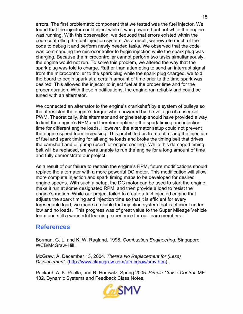
Figure 13. SMV Engine View #1 Figure 14. SMV Engine View #2

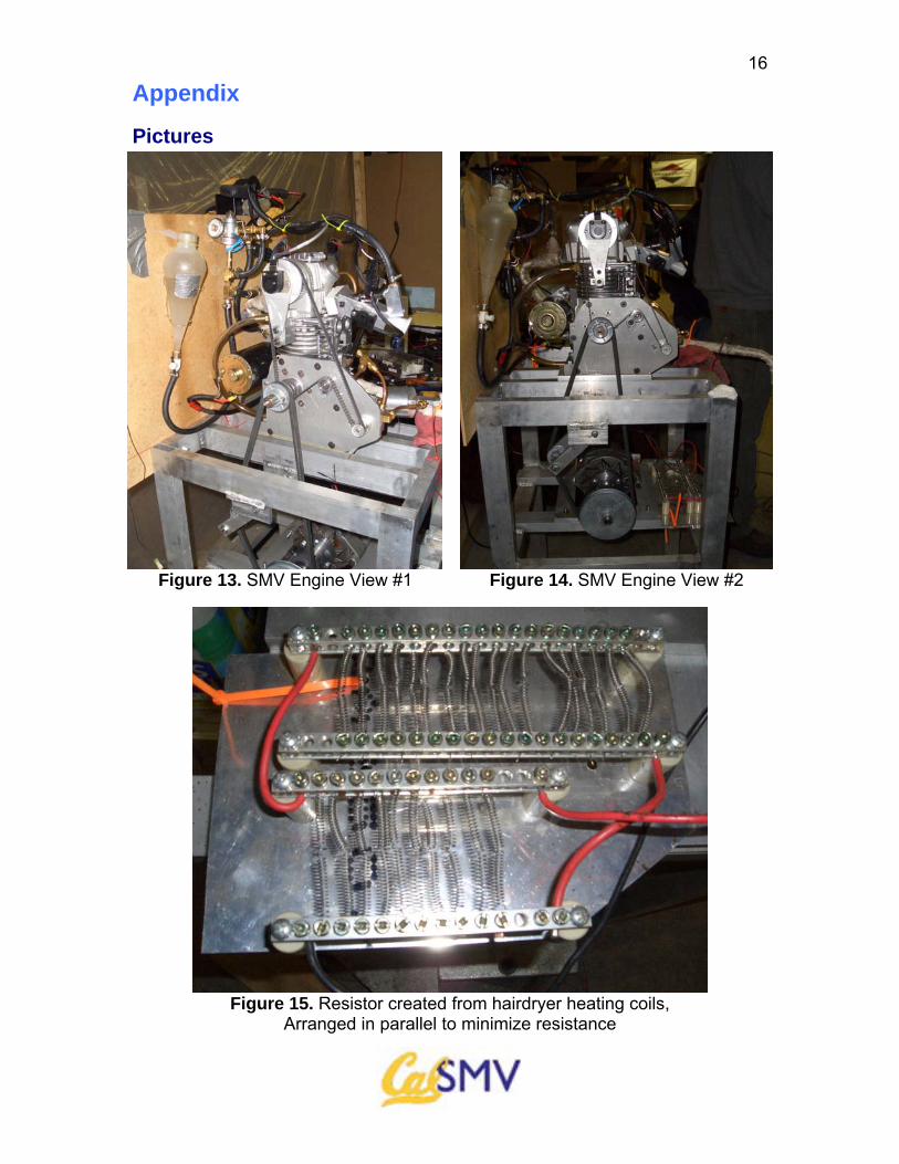
Figure 15. Resistor created from hairdryer heating coils,

Arranged in parallel to minimize resistance

17

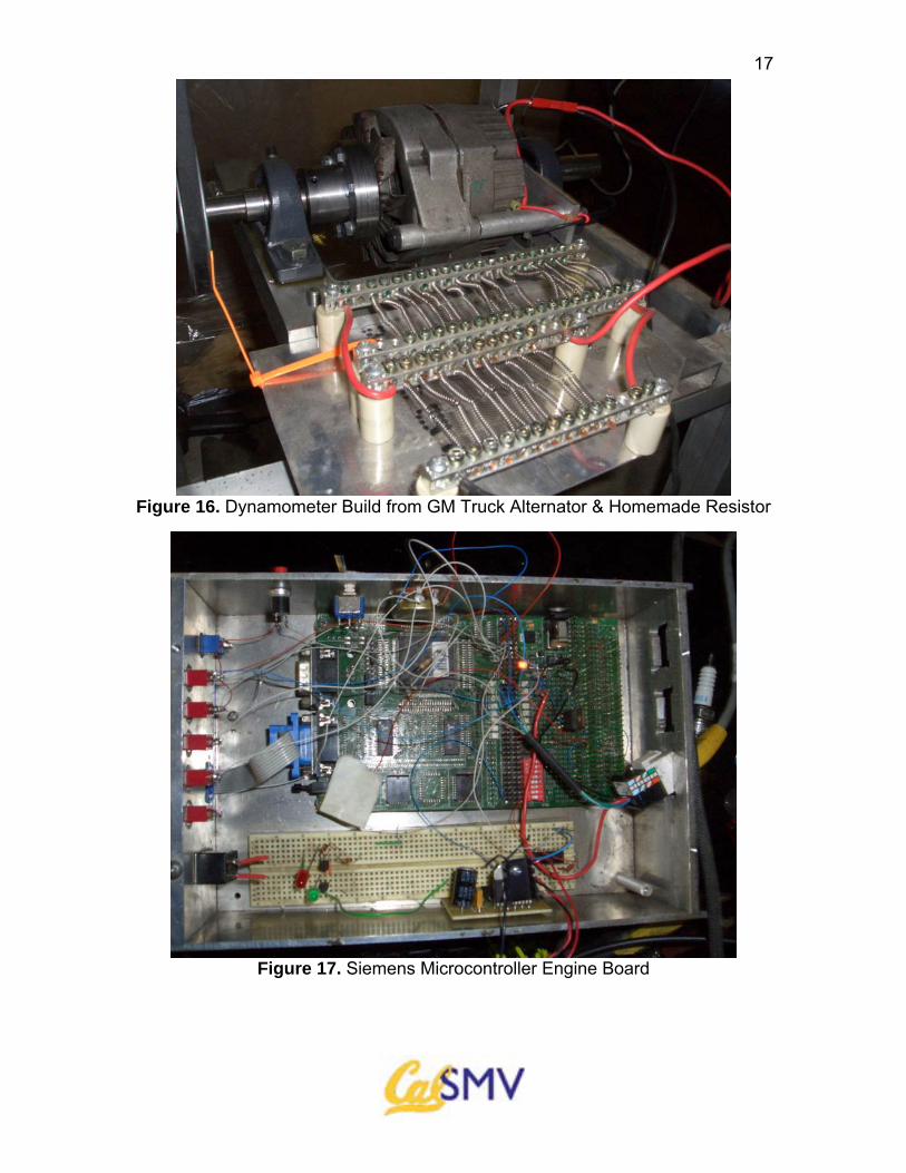
Figure 16. Dynamometer Build from GM Truck Alternator & Homemade Resistor

Figure 17. Siemens Microcontroller Engine Board

18

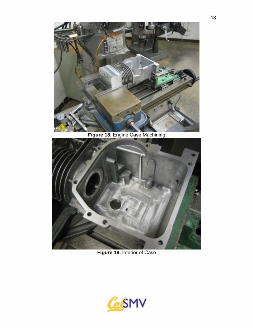
Figure 18. Engine Case Machining

Figure 19. Interior of Case