Calculating and graphing within-subject confidenceintervals for ANOVA

Thom Baguley

# Psychonomic Society, Inc. 2011

Abstract The psychological and statistical literature containsseveral proposals for calculating and plotting confidenceintervals (CIs) for within-subjects (repeated measures) ANOVAdesigns. A key distinction is between intervals supportinginference about patterns of means (and differences betweenpairs of means, in particular) and those supporting inferencesabout individual means. In this report, it is argued that CIs for theformer are best accomplished by adapting intervals proposed byCousineau (Tutorials in Quantitative Methods for Psychology,1, 42–45, 2005) and Morey (Tutorials in Quantitative Methodsfor Psychology, 4, 61–64, 2008) so that nonoverlapping CIs forindividual means correspond to a confidence for their differencethat does not include zero. CIs for the latter can beaccomplished by fitting a multilevel model. In situations inwhich both types of inference are of interest, the use of a two-tiered CI is recommended. Free, open-source, cross-platformsoftware for such interval estimates and plots (and for somecommon alternatives) is provided in the form of R functions forone-way within-subjects and two-way mixed ANOVA designs.These functions provide an easy-to-use solution to the difficultproblem of calculating and displaying within-subjects CIs.

Keywords Confidence intervals . ANOVA .Withinsubjects . Repeated measures . Displaying means .

Graphical methods

There is now widespread agreement among experts thatconfidence intervals (CIs) should replace or supplement the

reporting of p values in psychology (e.g., AmericanPsychological Association, 2010; Dienes, 2008; Loftus,2001; Rozeboom, 1960; Wilkinson & Task Force onStatistical Inference, 1999). What limited empirical datathere are (Fidler & Loftus, 2009) suggest that CIs are easierto interpret than p values (e.g., reducing common misinter-pretations associated with significance tests). In addition,there are a number of statistical arguments in favour ofreporting CIs—the chief one being that they are moreinformative, because they convey information about boththe magnitude of an effect and the precision with which ithas been estimated (Baguley, 2009; Loftus, 2001). Not allof the arguments in favour of reporting CIs are statistical.Even advocates of null-hypothesis significance tests havesuggested that such tests are overused, leading to “p valueclutter” (Abelson, 1995, p. 77). A plot of means with CIscould replace many of the less interesting omnibus tests andpairwise comparisons that routinely accompany ANOVA.

Despite this near consensus, it is not uncommon forstatistical summaries to be limited to point estimates—even for the most important effects. A major barrier toreporting CIs is lack of understanding among researchersof how to calculate an appropriate interval estimatewhere more than a single parameter estimate is involved.Cumming and Finch (2005) explored some of thesebarriers, providing guidance on how to calculate, report,and interpret CIs (with emphasis on the graphicalpresentation of means in a two-independent-group design).The difficulties they addressed are even more acute whenmore than two means are of interest or with within-subjects (repeated measures) designs.

In this article, I review the problem of constructing within-subjects CIs for ANOVA, consider the additional problem ofdisplaying the interval, review the main solutions that havebeen proposed, and propose guidelines for calculating anddisplaying appropriate CIs. These solutions are implemented

Electronic supplementary material The online version of this article(doi:10.3758/s13428-011-0123-7) contains supplementary material,which is available to authorized users.

T. Baguley (*)Division of Psychology, School of Social Sciences,Nottingham Trent University,Nottingham NG1 4BU, UKe-mail: Thomas.Baguley@ntu.ac.uk

DOI 10.3758/s13428-011-0123-7

Published online: 20 August 2011

Behav Res (2012) 44:158–175

in the software environment R for a one-way design, makingit easy to both obtain and plot suitable intervals. R is free,open source, and runs on Mac, Linux, and Windowsoperating systems (R Development Core Team, 2009). Thisprogram removes a barrier to the reporting of within-subjectsCIs: Few of the commonly proposed solutions are imple-mented in readily available software.

Within-subject confidence intervals: the natureof the problem

First, consider the simple case of constructing and plotting aCI around a single mean. In a typical application, the varianceis unknown and the interval estimate is formed using the tdistribution. Both the CI and the formally equivalent one-sample t test assume that data are sampled from a populationwith normally distributed, independent errors.1 For a sampleof size n, a two-sided CI with 100(1−α)% confidence takesthe formbm� tn�1;1�a=2 � bsbm; ð1Þ

where bm is the sample mean (and an estimate of thepopulation mean μ), tn�1;1�a=2 is the critical value of the tdistribution, and bsbm is the standard error of the meanestimated from the sample standard deviat ionbs ði:e:; bsbm ¼ bs= ffiffiffi

np Þ. The margin of error (CI half-width)

of this interval is therefore a multiple of the standard error ofthe parameter estimate. For intervals based on the tdistribution, this multiple depends on (a) sample size and(b) the desired level of confidence. The sample size has animpact on both sm and the critical value of t, but its impacton the latter is often negligible unless n is small (and for a95% CI, the multiplier tn–1,.975 approaches z.975 = 1.96 forany large sample).

In practice, researchers are often interested in comparingseveral means. ANOVA is the most common statisticalprocedure employed for this purpose. The additionalcomplexity of dealing with several independent meansproduces several challenges. Even for the simple case oftwo independent means (which reduces to an independent ttest), there are two main ways to plot an appropriate CI.The first option is to plot a CI for each population mean [e.g., using Eq. 1]. The second option is to plot a CI for thedifference in population means. For independent means μ1

and μ2, sampled from a normal distribution with unknownvariance, the CI for their difference takes the form

bm1 � bm2 � tn1þn2�2;1�a=2 � bsbm1�bm2; ð2Þ

where n1 and n2 are the sizes of the two samples and bsbm1�bm2is the standard error of the difference. This quantity istypically estimated from the pooled standard deviation ofthe samples as bsbm1�bm2

¼ bspooled

ffiffiffiffiffiffiffiffiffiffiffiffiffiffiffiffiffiffiffiffiffiffiffiffiffi1=n1 þ 1=n2

p. The only

additional assumption (at this stage) is that the populationvariances of the two groups are equal (i.e., s2

1 ¼ s22). A

crucial observation is that the standard error of thedifference is larger than the standard errors of the twomeans (bsbm1 and bsbm2

). This follows from the variance sumlaw, which relates the sum or difference of two variables totheir respective variances. For the variance of a difference,the relationship can be stated as

s2x1�x2

¼ s21 þ s2

2 � 2sx1�x2 ; ð3Þwhere sx1;x2 is the covariance between the two variables.Because the covariance is zero when the groups areindependent, s2

x1�x2reduces to s2

1 þ s22, and it follows that

the standard deviation of a difference isffiffiffiffiffiffiffiffiffiffiffiffiffiffiffiffis21 þ s2

2

p. If the

variances are also equal, it is trivial to show that thestandard error of a difference between independent means isffiffiffi2

ptimes larger than that of either of the separate means

(each standard error being a simple function of σ when n isfixed). Thus, if sample sizes and variances are approxi-mately equal, it is not unreasonable to work on the basisthat the standard error of any difference is around

ffiffiffi2

plarger

than the standard error for an individual parameter(Schenker & Gentleman, 2001).

This discrepancy presents problems when deciding whatto plot if more than one parameter (e.g., mean) is involved.Inference with a CI is usually accomplished merely bydetermining whether the interval contains or does notcontain a parameter value of interest (e.g., zero). Thispractice mimics a null-hypothesis significance test, but doesnot make use of the additional information a CI delivers. Abetter starting point is to treat values within the interval asplausible values of the parameter, and values outside theinterval as implausible values (Cumming & Finch, 2005;Loftus, 2001).2 Thus, the CI can be interpreted with respectto a range of potentially plausible parameter values, ratherthan restricting interest to a single value. This is veryimportant when considering the practical significance of aneffect (Baguley, 2009). For instance, a CI that excludes zeromay be statistically significant, but may not include anyeffect sizes that are practically significant. Likewise, a CIthat includes zero may be statistically nonsignificant, butthe effect cannot be interpreted as negligible unless it alsoexcludes nonnegligible effect sizes.

If the margin of error around each individual meancomputed from Eq. 1 is equal to 10, then the margin of

1 Alternatives exist that relax some or all of these assumptions, but arenot relevant to the present discussion.

2 Visual display of interval estimates lends itself to the informalinterpretation of a CI favoured here. CIs can also be used for formalinference, and if so, the same problems arise.

Behav Res (2012) 44:158–175 159

error around a difference between independent means willbe in the region of

ffiffiffi2

p � 10 � 14 (assuming similar samplesizes and variances). If the separate intervals overlap bysome minuscule quantity, then the total distance betweenthem will be approximately 10þ 10 ¼ 20. Since this gap islarger than 14, it is implausible, according to Eq. 2, that thetrue difference is zero. Plotting intervals around theindividual means using Eq. 1 will be misleading (e.g., ifthe overlapping CIs are erroneously interpreted as suggest-ing that the true difference might plausibly be zero).

It is possible to apply rules of thumb about theproportion of overlap to avoid these sorts of errors or toadjust a graphical display to deal with these problems(Cumming & Finch, 2005; Schenker & Gentleman, 2001).Furthermore, depending on the primary focus of inference,it is reasonable to plot the quantity of interest—whetherindividual means or their difference—with an appropriateCI. This is relatively easy with only two means, but withthree or more means it becomes harder. For instance, a plotof all of the differences between a set of means can be hardto interpret. Patterns that are obvious when plotting separatemeans (e.g., increasing or decreasing trends) will often beobscured.

The same general problems that arise when plotting CIsin between-subjects (independent measures) ANOVA alsoarise for within-subjects analyses. Plotting within-subjectsdata also raises a more fundamental problem. In a within-subjects design, it is no longer reasonable to assume thatthe errors in each sample are independent. It is almostinevitable that they will be correlated—and usually posi-tively correlated. The correlations reflect systematic indi-vidual differences that arise when measuring the same units(e.g., human participants) repeatedly. For example, partic-ipants with good memories will tend to score high on amemory task, leading to positive correlations betweenrepeated measurements. Negative correlations might ariseif repeated measurements are constrained by a commonfactor that forces some measurements to increase ordecrease at the expense of others (e.g., a fast response timemight slow down a later response if there is insufficienttime to recover between them).

The main implication of this dependence is that thestandard error for the differences between the means ofany two samples will depend on the correlation betweenthe two. This is evident from Eq. 3, bearing in mind thatthe Pearson correlation coefficient is a standardizedcovariance (i.e., rX1;X2

¼ sX1;X2=½sX1sX2 �). Positive corre-lations lead to smaller standard errors, while negativecorrelations lead to larger standard errors. Only if thecorrelation between measures is close to zero would oneexpect the standard error of a difference in a within-subjects design to be similar to that obtained with abetween-subjects design.

Within-subjects confidence intervals: some proposedsolutions

Loftus–Masson intervals In the psychological literature, thebest-known solution to the problem of plotting correlatedmeans in ANOVA designs is that of Loftus and Masson(1994; Masson & Loftus, 2003). Loftus and Massonrecognized the central problem of computing within-subjects confidence intervals in the context of ANOVA.They started by noting that plotting CIs around individualmeans in between-subjects designs is informative about thepattern of differences between conditions (because theirwidth is related by a factor of approximately

ffiffiffi2

pto the

width of a difference between means). In a between-subjects design, the typical approach is to use Eq. 1 tocalculate the standard error from a pooled standarddeviation rather than the separate estimates for each sample.This is readily derived from the between-subjects ANOVAerror term, because bspooled ¼

ffiffiffiffiffiffiffiffiffiffiffiffiffiffiMSerror

p. If sample sizes are

equal, this will produce intervals of identical width, butwhen sample sizes are unequal (or if homogeneity ofvariance cannot be assumed) researchers are advised tocompute the standard error separately for each sample. Inbalanced designs (those with equal cell sizes), this has theadded virtue of revealing systematic patterns in thevariances of the samples (e.g., increasing or decreasingwidth of the CI across conditions). However, because thepooled-variance estimate is based on all N observations,rather than on n within each of the J levels, the intervalswith separate error terms will be slightly wider (by virtue ofusing tn�1;1�a=2 as a multiplier rather than the valuetN�J ;1�a=2).

Loftus and Masson (1994) proposed a method ofconstructing a within-subjects CI that mimics the character-istics of the usual between-subjects CI for ANOVA. In abetween-subjects ANOVA, the individual differences aresubsumed in the error term of the analysis, and hencereduce the sensitivity of the omnibus F test statistic (thisbeing MSeffect/MSerror). Since the between-subjects CIsconstructed around individual means usually use the sameerror term as the omnibus F test, the two procedures arebroadly consistent. Clear patterns in a plot of means andCIs tend to be associated with a large F statistic. To createan equivalent plot for within-subjects CIs that is just asrevealing about the pattern of means between conditions,Loftus and Masson propose constructing the CI from thepooled error term of the within-subjects F statistic. Inessence, their approach is to adapt Eq. 1 by deriving spooled

from an error term that excludes systematic individualdifferences.

If individual differences are large relative to othersources of error, they can have a huge impact on the widthof the intervals that are plotted. Figure 1 shows data from a

160 Behav Res (2012) 44:158–175

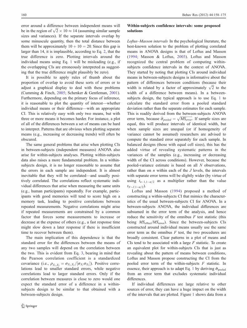
hypothetical free recall experiment reported by Loftus andMasson (1994), comparing three different presentationtimes (1, 2, or 5 s per word). The mean number of wordsrecalled (out of 25) is plotted in Fig. 1a as if they were froma between-subjects design and in Fig. 1b as if they arosefrom a within-subjects design.

Although the standard error used to construct the CI in eachpanel is based onMSerror, this is computed from the between-subjects ANOVA as

ffiffiffiffiffiffiffiffiffiffiffiffiffiffiffiffiffiffiffiffiffiMSwithin=N

pand from the within-

subjects ANOVA asffiffiffiffiffiffiffiffiffiffiffiffiffiffiffiffiffiffiffiffiffiffiffiffiffiffiffiffiffiffiffiMSfactor subjects=n

p.3 The dramatic

difference in widths in Fig. 1 is a consequence of the highcorrelation between repeated measurements on the sameindividuals (the correlations between pairs of measurementsfrom the same individual being in the region of r = .98 for thefree recall data). Real data might well produce less dramaticdifferences, but even the moderate correlations typical ofindividual differences between human participants (e.g., .20 <r < .80) are likely to have a substantial impact.

Loftus–Masson intervals are widely used, but haveattracted some criticism. They correctly mimic the relation-ship between the default CIs and the omnibus F test found forbetween-subjects designs, but they necessarily assumesphericity (homogeneity of variances of the differencesbetween pairs of repeated samples). The homogeneity-of-variances assumption is easy to avoid for between-subjectsCIs by switching from pooled to separate error terms, buttrickier to avoid for within-subjects CIs because the separateerror terms would still be correlated. Another concern is thatLoftus–Masson intervals are widely perceived as difficult tocompute and plot, and this has led to several publications

attempting to address these obstacles (e.g., Cousineau, 2005;Hollands & Jarmasz, 2010; Jarmasz & Hollands, 2009;Wright, 2007). A final issue is that Loftus–Masson intervalsare primarily concerned with providing a graphical repre-sentation of a pattern of a set of means for informalinference. They were never intended to mimic hypothesistests for individual means or for the differences betweenpairs of means. Loftus and Masson (1994; Masson & Loftus,2003) are quite explicit about this, and it would beunreasonable to criticize their approach on this basis.However, confusion arises in practice if the Loftus–Massonapproach is adopted and interpreted as a graphical imple-mentation of a significance test.

Cousineau–Morey intervals Cousineau (2005) proposed asimple alternative to Loftus–Masson CIs that does notassume sphericity. His approach also strips out individualdifferences from the calculation, but does this by normalizingthe data. This procedure was also used by Loftus and Masson(1994), but only to illustrate the process of removingindividual differences rather than for computing the CI.Indeed, at least one commentary on Loftus and Massonproposed constructing within-subjects CIs by normalizing theraw scores—though they refer to them as scores adjusted forbetween-subjects variability (Bakeman & McArthur, 1996).

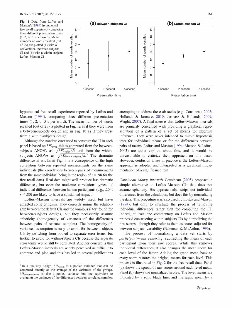
The process of normalizing a data set starts byparticipant-mean centering: subtracting the mean of eachparticipant from their raw scores. While this removesindividual differences, it also changes the mean score foreach level of the factor. Adding the grand mean back toevery score restores the original means for each level. Thisprocess is illustrated in Fig. 2 for the free recall data. Panel(a) shows the spread of raw scores around each level mean.Panel (b) shows the normalized scores. The level means areindicated by a solid black line, and the grand mean by a

3 In a one-way design, MSwithin is a pooled variance that can becomputed directly as the average of the variances of the groups.MSfactor×subjects is also a pooled variance, but one equivalent toaveraging the variances of the differences between correlated samples.

68

1012

1416

1820

(a) Between-subjects CI

Presentation time

Mea

n nu

mbe

r of

wor

ds r

ecal

led

Mea

n nu

mbe

r of

wor

ds r

ecal

led

1 second 2 second 5 second

68

1012

1416

1820

(b) Loftus-Masson CI

Presentation time

1 second 2 second 5 second

Fig. 1 Data from Loftus andMasson’s (1994) hypotheticalfree recall experiment comparingthree different presentation times(1, 2, or 5 s per word). Meannumbers of words recalled (outof 25) are plotted (a) with aconventional between-subjectsCI and (b) with a within-subjectsLoftus–Masson CI

Behav Res (2012) 44:158–175 161

dashed grey line. This combination of participant-meancentering followed by adding back the grand meanrelocates all condition effects relative to the grand meanrather than participant means.

Figure 2 illustrates how normalized scores relate allcondition effects relative to an idealized average participant(thus removing individual differences). This process couldalso be viewed as a form of ANCOVA in which adjustedmeans are calculated by stripping out the effect of abetween-subjects covariate (Bakeman & McArthur, 1996).Cousineau’s (2005) proposal is to use Eq. 1 to construct CIsfor the normalized samples. Because they are constructed inthe same way as standard CIs for individual means, it ispossible to use standard software to calculate and plot them(provided you first obtain normalized data). By removingindividual differences and computing CIs from a singlesample (without pooling error terms), there is also no needto assume sphericity.

Morey (2008) pointed out that Cousineau’s (2005)approach produces intervals that are consistently toonarrow. Morey explains that normalizing induces a positivecovariance between normalized scores within a condition,introducing bias into the estimates of the sample variances.The degree of bias is proportional to the number of means:For a one-way design with J means, a normalized varianceis too small by a factor of J/(J – 1). This suggests a simplecorrection to the Cousineau approach, in which the width ofthe CI is rescaled by a factor of

ffiffiffiffiffiffiffiffiffiffiffiffiffiffiffiffiffiffiffiffiJ � 1ð Þ=Jp

. For furtherdiscussion, and a formal derivation of the bias, see Morey’sstudy.

It is worth illustrating the process of constructing aCousineau–Morey interval in a little more detail. Thisillustration assumes a one-way within-subjects ANOVAdesign with J levels. If Yij is the score of the ith participantin condition j (for i = 1 to n), bmi is the mean of participant i

across all J levels (for j=1 to J), and bmgrand is the grandmean, normalized scores can be expressed as:

Y0ij ¼ Yij � bmi þ bmgrand: ð4Þ

The correct interval, removing the bias induced bynormalizing the scores, is therefore

bmj � tn�1;1�a=2

ffiffiffiffiffiffiffiffiffiffiffiffiJ

J � 1

r bs 0bmj; ð5Þ

where bs 0bmj is the standard error of the mean computed from

the normalized scores of the jth level. For factorial designs,Morey indicates that J can be replaced by the total number ofconditions across all repeated measures fixed factors (i.e.,excluding the random factor for subjects). In practice, thisinvolves computing the normalized scores of all repeatedmeasures conditions as if they arose from a one-way design.If the design also incorporates between-subjects factors, theintervals can be computed separately for each of the groupsdefined by combinations of between-subjects factors.

The intervals themselves have the same expected widthas the Loftus–Masson CIs in large samples, but do notassume sphericity. Except when J = 2, their width varies asa function of the variances and covariances of the repeatedmeasures samples (though when J = 2, the Cousineau–Morey and Loftus–Masson intervals are necessarily identi-cal). Because Cousineau–Morey intervals are sensitive tothe variances of the samples, they are therefore potentiallymore informative and more robust than Loftus–Massonintervals. This comes at a small cost. By abandoning apooled error term, the quantile used as a multiplier in Eq. 5is tn�1;1�a=2 rather than t n�1ð Þ J�1ð Þ;1�a=2. Thus, when J > 2,the Cousineau–Morey intervals will on average be slightlywider than Loftus–Masson intervals when n is small(though any given interval could be smaller or wider,

68

1012

1416

1820

(a) Raw scores

Presentation time

Mea

n nu

mbe

r of

wor

ds r

ecal

led

1 second 2 second 5 second

68

1012

1416

1820

(b) Normalized scores

Presentation time

Mea

n nu

mbe

r of

wor

ds r

ecal

led

1 second 2 second 5 second

Fig. 2 Normalized scoresremove individual differencesbut preserve the relationshipsbetween the level means (shownby a solid black line) and thegrand mean (shown by adashed grey line)

162 Behav Res (2012) 44:158–175

depending on the sample covariance matrix). As the aim isto produce intervals suitable for detecting patterns amongmeans when presented graphically, this cost can beconsidered negligible. A possible exception is for smallsamples (provided also that sphericity is not seriouslyviolated).

One further issue with the Cousineau–Morey intervals isthat correcting the normalized sample variance for biasintroduces an obstacle to calculating and plotting the CIs. Itis no longer possible simply to apply standard softwaresolutions to the normalized data. Cousineau (2005) pro-vides SPSS syntax for computing the uncorrected intervals.The correction factor can be incorporated into mostsoftware by a suitable adjustment of the confidence level.For moderately large samples and J = 2, a 99% CI for thenormalized scores gives an approximate 95% Cousineau–Morey interval. For instance, with α = .05 (i.e., 95%confidence) and n = 30, the usual critical value of t wouldbe 2.045. For a factor with J = 3 levels, the correction factoris

ffiffiffiffiffiffiffiffi3=2

p � 1:225. As 1.225×2.045≈2.5, you can mimic a95% Cousineau–Morey interval by plotting a 98.2% CI forthe normalized data using standard software. A 98.2% CI isrequired because t29 = 2.5 excludes around 0.9% in eachtail. It is possible to compute the required confidence levelusing most statistics packages or with spreadsheet software.The Appendix describes SPSS syntax for normalizing adata set and plotting Cousineau–Morey intervals.

Within-subjects intervals from a multilevel model Blouinand Riopelle (2005) presented a critique of Loftus–Massonintervals and proposed an alternative approach based onmultilevel (also termed linear mixed, hierarchical linear, orrandom coefficient) regression models. Multilevel modelswere developed to deal with clustered data such as childrenin schools (where children are modelled as Level 1 unitsnested within a random sample of schools at Level 2). Unitswithin a cluster tend to be more similar to each other thanunits from different clusters. In a multilevel model, thisdependency between observations is modelled by estimat-ing the variance within and between units as separateparameters. This differs from a standard linear regressionmodel, where a single variance parameter is estimated forthe individual differences. An important advantage ofmultilevel regression is the ability to extend the model todeal with dependencies arising from contexts other than asimple nested hierarchy with two levels. These includehierarchies with more than two levels, or different patternsof correlations between observations within a level. A morecomprehensive introduction to the topic is found in Hox(2010).

Blouin and Riopelle’s (2005) critique is quite technicaland has had limited impact (perhaps because it has beenpresented in relation to a particular software package: SAS,

SAS Institute, Cary, NC). The core of their critique is thatLoftus–Masson intervals, by stripping out individual differ-ences, derive CIs from a model in which subjects aretreated as a fixed factor. In contrast, a standard CI such asthose from Eqs. 1 or 2 (including the between-subjectsintervals that Loftus–Masson intervals seek to mimic) treatssubjects as a random effect. This implies that Loftus–Masson intervals cannot be legitimately applied for infer-ence about individual means. This may (at first) seem like adevastating critique of the Loftus–Masson approach. How-ever, a careful reading of Loftus and Masson (1994) revealsthat this conclusion is unwarranted; as already noted, Loftusand Masson are quite careful to restrict the interpretation oftheir intervals to an informal, graphical inference about thepattern of means.

Blouin and Riopelle (2005) confirmed this interpretationwhen they reported standard errors for the Loftus andMasson (1994) free recall data (plotted here in Fig. 1) bothfor an individual mean and for a difference between meanscomputed using their preferred method (a multilevel model).4

In their example, presentation time is treated as a fixed effect,subjects are a random effect, and a covariance matrix withcompound symmetry is fitted for the repeated measures (i.e.,for the within-subjects effect). Under this model, the standarderror for inference about an individual condition mean is1.879, but for a difference between means it is

ffiffiffi2

p � 0:248.The value of 0.248 is identical to the standard error of theLoftus–Masson interval. Inference about the pattern of means(implicitly linked to the differences between pairs of means)is therefore unaffected by the choice of ANOVA or multilevelmodel in this instance. This should not be surprising. Forbalanced data, there is a well-known equivalence between amultilevel model with compound symmetry among therepeated measures and a within-subjects ANOVA model,provided that restricted maximum likelihood (RML) estima-tion is used to fit the multilevel model (Searle, Casella, &McCulloch, 1992). The advantage of the multilevel model—with respect to inference about a pattern of means—istherefore its flexibility (Blouin & Riopelle, 2005; Hox, 2010;Searle et al., 1992). Within the multilevel framework, it isstraightforward to relax the sphericity assumption, to copewith unbalanced designs, and to incorporate additionalfactors or covariates.

The multilevel approach offers a flexible method forobtaining within-subjects CIs, both for revealing patterns ofmeans and for inferences about individual means. Theformer are more-or-less equivalent to either Loftus–Massonor Cousineau–Morey intervals (depending on the pattern of

4 Blouin and Riopelle (2005) frame the distinction in terms of the SASterminology “broad” or “narrow” inference spaces. However, in thiscase, the distinction (which is more general) boils down to inferenceabout means or differences in means. I assume most readers areunfamiliar with SAS terminology and attempt a simpler exposition.

Behav Res (2012) 44:158–175 163

variances and covariances being assumed). The latter arearguably superior to those constructed from individualsamples (Blouin & Riopelle, 2005).

Goldstein–Healy plots The problem of the graphical presen-tation of means (or indeed of other statistics such as oddsratios) occurs in contexts other than classical ANOVA designs.Goldstein and Healy (1995) proposed a simple solutiondesigned for presenting a large collection of means. Theirsolution was intended to facilitate inference about differencesbetween pairs of statistics—its best-known application beingin the effectiveness of schools (e.g., by plotting estimates ofLevel 2 residuals for a multilevel model comparingeducational attainment of children clustered within schools).The basic form of the proposal is to derive a commonmultiplier to the standard errors of each statistic that, whenplotted, would equate to an approximate 95% CI for theirdifference. This multiplier combines the appropriate quantileand the requisite adjustment for a difference betweenindependent means into a single number, thus facilitatingplotting of a large number of statistics (assuming that thestandard errors are available).5

Goldstein and Healy (1995) showed that for twoindependent means sampled from normal distributions withknown standard errors, the probability of nonoverlappingCIs with 100(1 – α) = C% confidence is given by

gij ¼ 2 1� Φ zCsbmi

þ sbmjffiffiffiffiffiffiffiffiffiffiffiffiffiffiffiffiffiffis2bmi

þ s2bmj

q0B@

1CA264

375: ð6Þ

In this equation, sbmiand sbmj

are the standard errors of themeans, and zC is the positive quantile of the standardnormal distribution z that corresponds to C% confidence.When these two standard errors are equal, the quantitysbmi þ sbmj� �

=ffiffiffiffiffiffiffiffiffiffiffiffiffiffiffiffiffiffis2bmi

þ s2bmj

qis at its maximum and γij is at its

minimum. Conversely, γij is maximized when one standard

error is infinitely larger than the other (e.g., smi¼ 0 and

smj¼ 1). Fixing γij at the desired probability and solving

for zC gives the appropriate multiplier for a plot of the twomeans. This logic can be extended to other statistics. Thequantity sbmi þ sbmj� �

=ffiffiffiffiffiffiffiffiffiffiffiffiffiffiffiffiffiffis2bmi þ s2bmjq

can be averaged over all

pairs when plotting more than two statistics (and thisapproach will be reasonably accurate, unless the range ofstandard errors is large).

A multiplier of approximately 1.39 standard errorsproduces approximate 95% CIs of the difference between

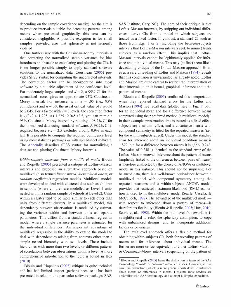
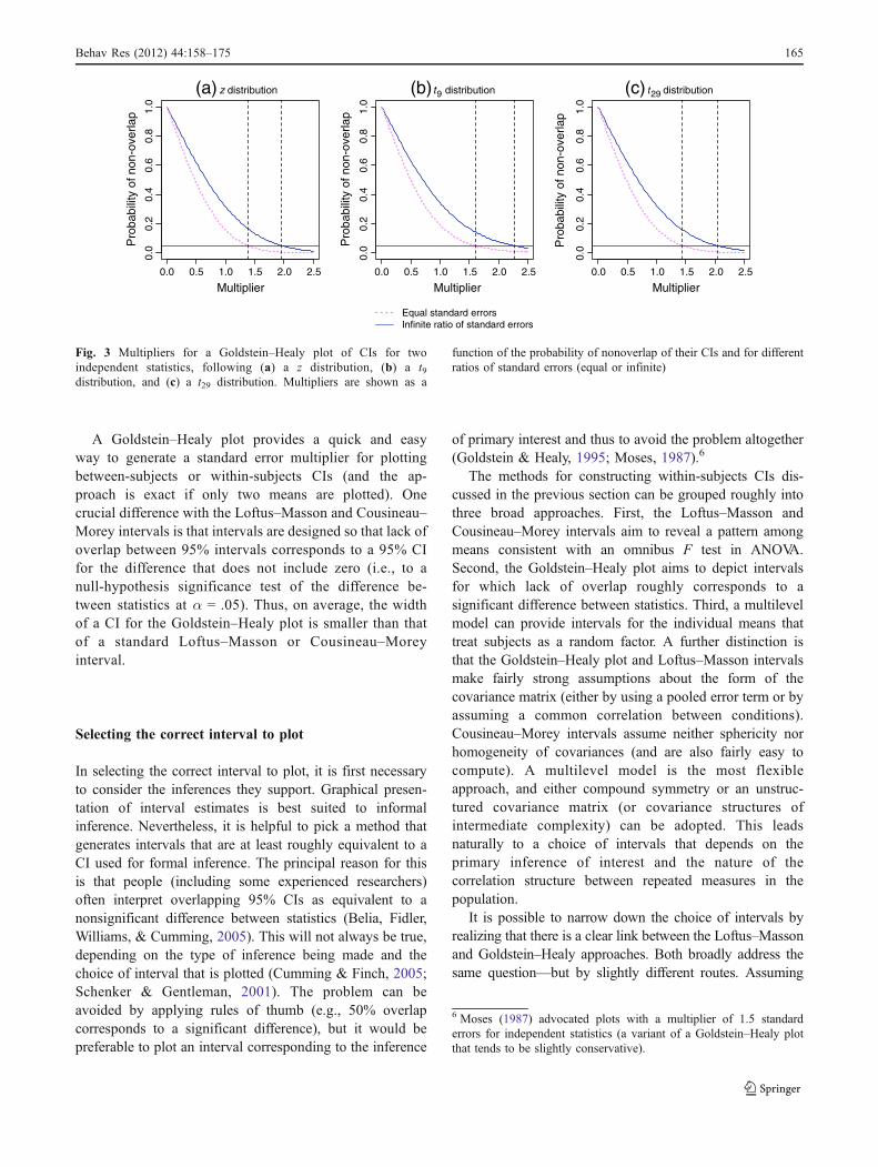
independent statistics with equal standard errors (Goldstein& Healy, 1995). Panel (a) of Fig. 3 plots the probability ofnonoverlap γij as a function of the right-hand side of Eq. 6.This is done separately for the smallest ratio of standarderrors and for maximally different standard errors. Thehorizontal line at γij = .05 intersects these lines at 1.386 (tothree decimal places) for the equal-standard-errors curve, or1.960 if the ratio of standard errors is infinitely large (or if itapproaches zero). The latter necessarily reduces to amultiplier for a single mean (the other mean being, ineffect, a population parameter measured with perfectprecision). The extension to the t distribution is straightfor-ward (Afshartous & Preston, 2010; Goldstein & Healy,1995), in which case the multiplier also varies as a functionof the degrees of freedom (df). This can be seen in panels(b) and (c) of Fig. 3, where the function for nonoverlap of aCI is shown for t distributions with 9 and 29 df,respectively. The t distribution converges rapidly on z asits df become large. Thus, the z approximation is likely tobe adequate, even if the standard errors are estimatedfrom the sample standard deviation (provided that n is notvery small).

For within-subjects CIs, it would be unreasonable toassume independent statistics. Afshartous and Preston(2010) consider how to construct a Goldstein–Healy plotfor correlated statistics. The sbmi þ sbmj term in Eq. 6 isderived from the variance sum law when the covariancebetween sample statistics is exactly zero (representing thestandard error of a difference between the statistics).Expressing Eq. 3 in terms of the standard errors of thestatistics and the correlation between the samples ρij andapplying this to Eq. 6 gives the corresponding expressionfor within-subjects CIs,

gij ¼ 2 1� Φ zCsbmi

þ sbmjffiffiffiffiffiffiffiffiffiffiffiffiffiffiffiffiffiffiffiffiffiffiffiffiffiffiffiffiffiffiffiffiffiffiffiffiffiffiffiffiffiffiffis2bmi

þ s2bmj

� 2rijsbmisbmj

q0B@

1CA264

375: ð7Þ

With this equation, the average correlation between pairs ofrepeated measures could be used alongside the averageratio of standard errors to generate a single multiplier for aset of correlated means or other statistics. Afshartous andPreston (2010) explained how to calculate multipliers forwithin-subjects or between-subjects CIs using the z or tdistribution. Unlike variability in standard errors or thechoice of t or z, whether the statistics are independent orcorrelated has a huge impact on the multiplier. For instance,a modest positive correlation of ρij = .30 reduces themultiplier from around 1.446 to 1.210 for a t distributionwith df = 29. For the same sample size, ρij = .75 halves thewidth of the CI in relation to the independent case (from1.446 to 0.7231).

5 A plot involving such a large number of statistics is sometimestermed a caterpillar plot—for its resemblance to the insect. The termGoldstein–Healy plot is preferred here (because the focus is onplotting intervals for a small number of means for which theresemblance is typically lost).

164 Behav Res (2012) 44:158–175

A Goldstein–Healy plot provides a quick and easyway to generate a standard error multiplier for plottingbetween-subjects or within-subjects CIs (and the ap-proach is exact if only two means are plotted). Onecrucial difference with the Loftus–Masson and Cousineau–Morey intervals is that intervals are designed so that lack ofoverlap between 95% intervals corresponds to a 95% CIfor the difference that does not include zero (i.e., to anull-hypothesis significance test of the difference be-tween statistics at α = .05). Thus, on average, the widthof a CI for the Goldstein–Healy plot is smaller than thatof a standard Loftus–Masson or Cousineau–Moreyinterval.

Selecting the correct interval to plot

In selecting the correct interval to plot, it is first necessaryto consider the inferences they support. Graphical presen-tation of interval estimates is best suited to informalinference. Nevertheless, it is helpful to pick a method thatgenerates intervals that are at least roughly equivalent to aCI used for formal inference. The principal reason for thisis that people (including some experienced researchers)often interpret overlapping 95% CIs as equivalent to anonsignificant difference between statistics (Belia, Fidler,Williams, & Cumming, 2005). This will not always be true,depending on the type of inference being made and thechoice of interval that is plotted (Cumming & Finch, 2005;Schenker & Gentleman, 2001). The problem can beavoided by applying rules of thumb (e.g., 50% overlapcorresponds to a significant difference), but it would bepreferable to plot an interval corresponding to the inference

of primary interest and thus to avoid the problem altogether(Goldstein & Healy, 1995; Moses, 1987).6

The methods for constructing within-subjects CIs dis-cussed in the previous section can be grouped roughly intothree broad approaches. First, the Loftus–Masson andCousineau–Morey intervals aim to reveal a pattern amongmeans consistent with an omnibus F test in ANOVA.Second, the Goldstein–Healy plot aims to depict intervalsfor which lack of overlap roughly corresponds to asignificant difference between statistics. Third, a multilevelmodel can provide intervals for the individual means thattreat subjects as a random factor. A further distinction isthat the Goldstein–Healy plot and Loftus–Masson intervalsmake fairly strong assumptions about the form of thecovariance matrix (either by using a pooled error term or byassuming a common correlation between conditions).Cousineau–Morey intervals assume neither sphericity norhomogeneity of covariances (and are also fairly easy tocompute). A multilevel model is the most flexibleapproach, and either compound symmetry or an unstruc-tured covariance matrix (or covariance structures ofintermediate complexity) can be adopted. This leadsnaturally to a choice of intervals that depends on theprimary inference of interest and the nature of thecorrelation structure between repeated measures in thepopulation.

It is possible to narrow down the choice of intervals byrealizing that there is a clear link between the Loftus–Massonand Goldstein–Healy approaches. Both broadly address thesame question—but by slightly different routes. Assuming

0.0 0.5 1.0 1.5 2.0 2.5 0.0 0.5 1.0 1.5 2.0 2.5 0.0 0.5 1.0 1.5 2.0 2.5

0.0

0.2

0.4

0.6

0.8

1.0

(a) z distribution

Multiplier Multiplier Multiplier

Pro

babi

lity

of n

on-o

verla

p

0.0

0.2

0.4

0.6

0.8

1.0

(b) t9 distribution

Pro

babi

lity

of n

on-o

verla

p

Equal standard errorsInfinite ratio of standard errors

0.0

0.2

0.4

0.6

0.8

1.0

(c) t29 distribution

Pro

babi

lity

of n

on-o

verla

p

Fig. 3 Multipliers for a Goldstein–Healy plot of CIs for twoindependent statistics, following (a) a z distribution, (b) a t9distribution, and (c) a t29 distribution. Multipliers are shown as a

function of the probability of nonoverlap of their CIs and for differentratios of standard errors (equal or infinite)

6 Moses (1987) advocated plots with a multiplier of 1.5 standarderrors for independent statistics (a variant of a Goldstein–Healy plotthat tends to be slightly conservative).

Behav Res (2012) 44:158–175 165

large samples with equal variances and covariances, theexpected width of both Loftus–Masson and Cousineau–Morey intervals is larger than that of the interval in aGoldstein–Healy plot by the familiar factor of

ffiffiffi2

p. It is

therefore simple to adjust either interval to match the other.Because the Cousineau–Morey intervals assume neithersphericity nor homogeneity of covariances for the repeatedmeasures they should, as a rule, be preferred over the othertwo methods. Sphericity only infrequently holds for real datasets (with the exception of within-subjects ANOVA effectswith 1 df in the numerator—equivalent to a paired t test—forwhich sphericity is always true). Because violations ofsphericity always lead to inferences that are too liberal(e.g., CIs that are too narrow), it makes sense to chooseinterval estimates that relax the assumption by default.

For inferences about differences in means that areconsistent with the omnibus F test from within-subjectsANOVA, and for which nonoverlap of CIs corresponds toan inference of no difference, I propose plotting Cousineau–Morey intervals with the following adjustment:

bmj �ffiffiffi2

p

2tn�1;1�a=2

ffiffiffiffiffiffiffiffiffiffiffiffiJ

J � 1

r bs 0bmj

!

¼ bmj � tn�1;1�a=2

ffiffiffiffiffiffiffiffiffiffiffiffiffiffiffiffiffiffi2J

4 J � 1ð Þ

s bs 0bmj: ð8Þ

Theffiffiffi2

p=2 factor adjusts a Loftus–Masson or Cousineau–

Morey interval to match that of a CI for a difference (see, e.g.,Hollands & Jarmasz, 2010). This equation combines advan-tages of computing a standard error from normalized data withthe ease of interpretation of CIs in a Goldstein–Healy plot.

It is worth making the reasoning behind theffiffiffi2

p=2

adjustment factor explicit. Although the ratio of the widthof the CI for a difference to the CI for an individual mean isffiffiffi2

pto 1, this must be halved when plotting intervals around

individual means. For a difference in means, inferencedepends on the margin of error around one statisticincluding or not including a parameter value (e.g., zero).Lack of overlap of CIs plotted around individual meansdepends on the margin of error around two statistics. Toensure that the sum of the margin of error around eachstatistic is

ffiffiffi2

ptimes larger than for an individual statistic, it

is necessary to scale each individual margin of error (w) bythe

ffiffiffi2

p=2 factor (i.e.,

ffiffiffi2

p=2wþ ffiffiffi

2p

=2w ¼ ffiffiffi2

pw). The

halving is therefore a trivial, but easily overlooked,consequence of plotting two intervals rather than one.

In some cases, it may be reasonable to plot an adjustedLoftus–Masson interval instead. For a one-way within-subjects ANOVA, this takes the form

bmj �ffiffiffi2

p

2� t n�1ð Þ J�1ð Þ;1�a=2

ffiffiffiffiffiffiffiffiffiffiffiffiffiffiffiMSerror

n

r; ð9Þ

where MSerror is the denominator of F statistic for the test ofthe factor. When sphericity holds, Eq. 9 offers a modestadvantage over Eq. 8 when n – 1 is small (e.g., below 15)and (n – 1)(J – 1) is large (e.g., over 30). Note that Eq. 9also explains the correspondence between the Goldstein–Healy plot and adjusted Loftus–Masson intervals. Themultiplier in the former combines the

ffiffiffi2

p2= adjustment

and the quantile t n�1ð Þ J�1ð Þ;1�a=2 in the latter (ffiffiffiffiffiffiffiffiffiffiffiffiffiffiffiffiffiffiffiMSerror=n

pbeing the standard error). One further distinction is that theLoftus–Masson intervals deal with within-subjects designsby removing individual differences from the standard error.The spirit of the Goldstein–Healy plot is to adjust only themultiplier, and thus Afshartous and Preston (2010) recal-culate the multiplier of the Goldstein–Healy plot to takeaccount of the correlation between the standard errors.

For many applications of ANOVA, it is sufficient tofocus on the pattern of means and differences between pairsof means. In this case, the adjusted Cousineau–Moreyinterval proposed here is a sensible candidate. In someapplications of ANOVA, the primary focus will be oninference about individual means. This might arise in alongitudinal study where the focus is on whether the meanis different from some threshold at each time point. If so, itwould be more appropriate to plot CIs derived from amultilevel model. One of the advantages of this approach isthe ability to relax the sphericity assumption by fitting amodel with an unstructured covariance matrix (estimatingthe variances and covariances between repeated measureswith separate parameters).

I have suggested that inference about individual means isonly infrequently the main focus of inference for ANOVAdesigns. Nevertheless, there will almost always be someinterest in the width of the CI for the individual means. Forexample, in a recognition memory experiment, the mainfocus will usually be on differences between conditions, butit would also be valuable to ascertain whether performancein each condition exceeds chance. The width of a CI for anindividual mean also indicates the precision with which thatstatistic has been measured (Kelley, Maxwell, & Rausch,2003; Loftus, 2001). For this reason alone, it would beadvantageous to be able to display CIs representing differ-ences between means alongside those depicting the preci-sion with which each sample is measured. Simultaneousplotting of two distinct interval estimates can be addressedin several ways, but perhaps the most elegant and user-friendly display is a two-tiered CI: a form of two-tierederror bar plot (Cleveland, 1985).

The outer tier of a two-tiered CI is plotted as a standarderror bar. The inner tier is then formed by drawing a line atright angles to the error bar with the required margin oferror (as if shifting the line commonly drawn at the limits ofthe interval so that it bisects the error bar). Cleveland(1985) used the inner tier of the error bar to designate a

166 Behav Res (2012) 44:158–175

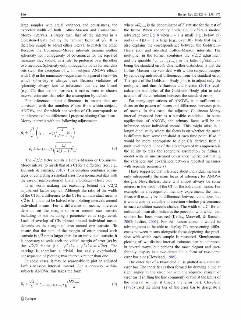
50% CI (similar to the central box of a box plot), while theouter tier represented a 95% CI for each statistic. I proposeusing the outer tier to depict a 95% CI for an individualmean and drawing the inner tier so that lack of overlapcorresponds to a 95% CI for the difference in means. Thisproperty is demonstrated in Fig. 4, in which two-tiered CIsfor the difference between two correlated means aredisplayed.

In panel (a), the correlation between paired observations issubstantial (r = .8) and a paired t test is statisticallysignificant (p = .001). In panel (b), the correlation betweenpaired observations is lower (r = .6) and the paired t test ison the cusp of statistical significance (p = .05). In panel (c),the correlation between paired observations is lower still (r =.45) and the paired t test is nonsignificant (p = .10). Figure 4demonstrates the close correspondence between overlap ofthe inner error bars and statistical significance from a paired ttest (and, by implication, a CI for a difference that includeszero as a plausible value).

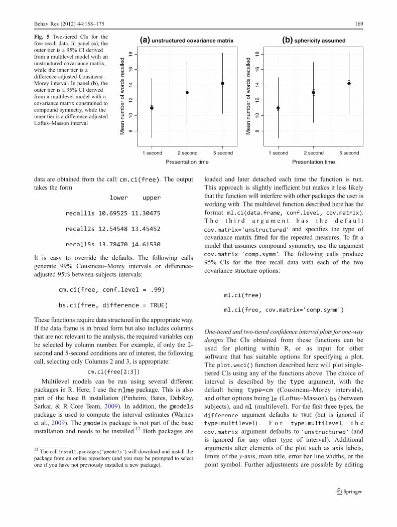
Figure 5 depicts two-tiered CIs for the free recall dataconstructed in this way. Panel (a) plots 95% CIs from amultilevel model with an unstructured covariance matrixfor the outer tier and difference-adjusted Cousineau–Moreyintervals for the inner tier. Panel (b) plots 95% CIs from amultilevel model under the assumption of compoundsymmetry for the repeated measures as the outer tier anddifference-adjusted Loftus–Masson intervals for the innertier.

For these data, the correlations between repeatedmeasures are both very high and very consistent. Itfollows that both constrained and unconstrained covari-ance matrix approaches will produce similar results. Thisis the case even though n = 10 (which implies that theLoftus–Masson intervals are on average slightly narrowerthan the Cousineau–Morey intervals).7 Looking at thetwo-tiered CI, the presence of plausible differencesbetween the conditions—indicated by nonoverlappinginner error bars—is obvious. Also obvious is the lack ofprecision with which individual means are measured. Sowhile the experiment provides clear evidence of differ-ences between conditions, it is also clear that participantsvary considerably on this task and that each populationmean is estimated very imprecisely.

The recipe for construction of a two-tiered CIdescribed here is suitable when—as is common—thecorrelation between the samples is positive. If some

covariances are negative or if sample sizes are verysmall, the recipe could fail: The (outer) multilevel CImay be narrower than the (inner) difference-adjusted CI.When n for one or more samples is very low (e.g., <10),the quality of the variance and covariance estimates islikely to be poor. A pooled error term is likely to providesuperior estimates in this situation (particularly if negativecorrelations have arisen through sampling error). In largersamples, any negative correlations are likely to reflect aprocess of genuine interest to a researcher, and it may bebetter to plot the individual means and differencesseparately (even if adopting a pooled error term producesa “successful” two-tiered CI plot).8

Constructing one-tiered and two-tiered confidenceinterval plots

Cousineau–Morey CIs can be computed from standardANOVA output without too much difficulty (e.g., usingspreadsheet software such as Excel). Single-tier CI plotscan be generated with a little more effort. Many statisticalpackages, such SPSS, also have options to fit multilevelmodels for within-subjects ANOVA designs and canprovide appropriate CIs for individual means. Constructinga two-tier plot is more difficult. To facilitate this process forone-tier plots and to support the use of two-tiered plots, it ispossible to write custom macros or functions. This sectionintroduces R functions for computing and plotting one-tiered and two-tiered plots for Loftus–Masson, Cousineau–Morey, and multilevel model intervals (R DevelopmentCore Team, 2009). I provide the code for new R functionsto compute the CIs and construct the plots in thesupplementary materials for this article. Other functionsused here are loaded automatically with R or are part of theR base installation. Their application is illustrated first for aone-way within-subjects design. For the Cousineau–Moreyand multilevel model approaches, it is also extended todeal with two-way mixed designs. R was chosen becauseit is free, open source, and runs on Mac, Windows, andLinux operating systems. This removes a further obstaclepreventing researchers from graphical presentation ofmeans from within-subjects ANOVA designs. Goldstein–Healy plots, more suited to large collections of means

7 In moderate to large samples, true coverage for the two intervals shouldbe very similar when sphericity is true (and close to nominal coverage forsamples from populations with normal errors), but for even quite modestviolations of sphericity, the coverage of Loftus–Masson intervals is likelyto unacceptable (see Mitzel & Games, 1981).

8 In most cases where the “inner” tier error bars fall outside the rangeof the “outer” tier, the bars fall close to the ends of the vertical linerepresenting the multilevel CI and appear coherently “grouped.” Thisunusual variant of the two-tiered plot is still interpretable (and can actas a diagnostic for the presence of negatively correlated samples). Rcode illustrating such a plot is included in the supplementary materialspublished with this article.

Behav Res (2012) 44:158–175 167

and other statistics, are not implemented. However,Afshartous and Preston (2010) have provided R functionsfor calculating multipliers for between-subjects (indepen-dent) and within-subjects (dependent) designs for both zand t distributions.

Confidence intervals for one-factor ANOVA designs Thefollowing examples use the free recall data from Loftus andMasson (1994). This data set and the emotion data set used inlater examples are included in the supplementary materials.The first step is to load the data into R. Two options areillustrated here. The first assumes that the data set is in theform of a comma-separated variable (.csv) file. The secondassumes that data are in an SPSS (.sav) data file. R functionsusually take within-subjects (repeated measures) data in longform, with each observation on a separate row, but mostANOVA software requires the data in broad form (where eachperson is on a separate row).9 Data imported from othersoftware will therefore usually arrive in broad format. For thisreason, the R functions described here take input as a dataframe (effectively a collection of named variables arranged incolumns) in broad form. The file is arrangedin three columns so that the first row contains the threecondition names ( , and ) and thenext 10 rows contain the raw data. To import data from thisfile, type at the R con-sole prompt and then hit the return key.10 R will import the

data into the data frame and use the header row ascolumn names. If the data are in an SPSS .sav file, it is firstnecessary load the package (a part of the baseinstallation that allows for importing of data from otherpackages). The following commands use thefunction to import the data:

The additional argument overrides thedefault behaviour of the function (which is to import data asan R list object).

For one-way ANOVA, the functionsand provide between-subjects, Loftus–Masson,and Cousineau–Morey intervals, respectively.11 Each is struc-tured in the format

. The first argument is the name ofthe R data frame object containing the data in broad format(and must be included). The second argument is the desiredconfidence level, and defaults to .95 (95%) if omitted. Thethird argument takes the value or and indicateswhether to adjust the width of the interval so thatabsence of overlap of CIs for two means corresponds toa 95% CI for their difference. It defaults to for

and , and for . To calleach function with its default settings, use the format

. For example, difference-adjusted 95% Cousineau–Morey intervals for the free recall

68

1012

14

68

1012

14

68

1012

14

(a) (b) (c)tt14 = 4.14, p = .001

Con

fiden

ce in

terv

al fo

r m

ean

1 2 1 2 1 2

t14 = 2.14, p = .05

Con

fiden

ce in

terv

al fo

r m

ean

t14 = 1.75, p = .10

Con

fiden

ce in

terv

al fo

r m

ean

Fig. 4 Overlap of the inner-tier error bars of a two-tiered 95% CIcorresponds to statistical significance with α = .05 and indicates thatthe 95% CI for a difference includes zero. In panel (a), there is clearseparation of the inner-tier error bars, and the paired t test isstatistically significant (p < .05). In panel (b), the inner-tier error bars

are adjacent, and the paired t test is on the cusp of statisticalsignificance (p = .05). In panel (c), the inner-tier error bars showsubstantial overlap, and the paired t test does not reach statisticalsignificance (p > .05)

9 Switching between long and broad forms can be accomplished usingthe function in R. SPSS users can restructure the data setusing the command.

11 The between-subjects CI function is implemented primarily forpurposes of comparison. It uses a pooled variance estimate and alsoonly takes input in broad format (rather than the usual long format).

10 R will import files from its working directory. If the data are not inthis directory, either change the working directory or specify the fullpath name (not illustrated here because it depends on the operatingsystem).

168 Behav Res (2012) 44:158–175

data are obtained from the call: . The outputtakes the form

It is easy to override the defaults. The following callsgenerate 99% Cousineau–Morey intervals or difference-adjusted 95% between-subjects intervals:

These functions require data structured in the appropriate way.If the data frame is in broad form but also includes columnsthat are not relevant to the analysis, the required variables canbe selected by column number. For example, if only the 2-second and 5-second conditions are of interest, the followingcall, selecting only Columns 2 and 3, is appropriate:

Multilevel models can be run using several differentpackages in R. Here, I use the package. This is alsopart of the base R installation (Pinheiro, Bates, DebRoy,Sarkar, & R Core Team, 2009). In addition, thepackage is used to compute the interval estimates (Warneset al., 2009). The package is not part of the baseinstallation and needs to be installed.12 Both packages are

loaded and later detached each time the function is run.This approach is slightly inefficient but makes it less likelythat the function will interfere with other packages the user isworking with. The multilevel function described here has theformat .T h e t h i r d a r g u m e n t h a s t h e d e f a u l t

and specifies the type ofcovariance matrix fitted for the repeated measures. To fit amodel that assumes compound symmetry, use the argument

. The following calls produce95% CIs for the free recall data with each of the twocovariance structure options:

One-tiered and two-tiered confidence interval plots forone-waydesigns The CIs obtained from these functions can beused for plotting within R, or as input for othersoftware that has suitable options for specifying a plot.The function described here will plot single-tiered CIs using any of the functions above. The choice ofinterval is described by the argument, with thedefault being (Cousineau–Morey intervals),and other options being (Loftus–Masson), (betweensubjects), and (multilevel). For the first three types, the

argument defaults to (but is ignored if) . F o r , t h e

argument defaults to (andis ignored for any other type of interval). Additionalarguments alter elements of the plot such as axis labels,limits of the y-axis, main title, error bar line widths, or thepoint symbol. Further adjustments are possible by editing

810

1214

1618

810

1214

1618

(a) unstructured covariance matrix

Presentation time

Mea

n nu

mbe

r of

wor

ds r

ecal

led

1 second 2 second 5 second 1 second 2 second 5 second

(b) sphericity assumed

Presentation time

Mea

n nu

mbe

r of

wor

ds r

ecal

led

Fig. 5 Two-tiered CIs for thefree recall data. In panel (a), theouter tier is a 95% CI derivedfrom a multilevel model with anunstructured covariance matrix,while the inner tier is adifference-adjusted Cousineau–Morey interval. In panel (b), theouter tier is a 95% CI derivedfrom a multilevel model with acovariance matrix constrained tocompound symmetry, while theinner tier is a difference-adjustedLoftus–Masson interval

12 The call will download and install thepackage from an online repository (and you may be prompted to selectone if you have not previously installed a new package).

Behav Res (2012) 44:158–175 169

the plot or altering the plot parameters in R. The followingcommands reproduce panels (a) and (b) of Fig. 1:

The default behaviour of the function is to produce theoption recommended here: a Cousineau–Morey CI with anadjustment, so that nonoverlapping intervals correspond tothe 95% CI for their difference. Thus, the following twocalls are equivalent:

The composition of a tiered plot is less flexible. Itmakes sense to pair multilevel-model CIs with anunstructured covariance matrix to Cousineau–Moreyintervals. Likewise, it makes sense to pair a multilevel-model CI that assumes compound symmetry to Loftus–Masson intervals. The interval type is determined by the

argument. The former is the default output( ) , whi le the la t t e rrequires the argument . The

argument influences only the inner tier andadjusts either the Cousineau–Morey or Loftus–Massonintervals by the

ffiffiffi2

p=2 factor required to support infer-

ences about differences between means. As before, this isset by the argument (which is thedefault).

As for the function, additional argumentscan be supplied to influence the look of the plot or altertitles and labels. The function also takesthree further arguments: for the size of the pointsbeing plotted, for the size of text labels, and

or (to add a grid to the plot).The grid is particularly useful for a complex two-tieredplot, where the grid can make it easier to detect overlap.

Thus panels (a) and panel (b) of Fig. 5 can be reproducedwith the following R code:

A basic two-tiered plot (with Cousineau–Morey intervalsfor differences between means as the inner tier andmultilevel CIs with an unstructured covariance matrix asthe outer tier) is therefore obtained by:

To augment the display, plotting parameters can be editedusing the function, and lines or other features addedto the plot using , or oneof many other R graphics functions.13 Hence, to add dashedlines (line type ) connecting the level means to thefree recall plot, either of these functions will work:

13 To find out more about any function in the R base installation, usethe function or . The call or bringsup information about the graphical parameters.

170 Behav Res (2012) 44:158–175

Functions for two-way mixed ANOVA designs Obtainingintervals for more complex designs using the Cousineau–Morey or multilevel approaches is not too difficult in R.The principal obstacle is to rewrite the functions to pickout a grouping variable from a data frame in broadformat. Deciding how to plot the intervals is morechallenging. The functions in this section demonstrateone solution to plotting the intervals. This is implementedfor the two-tiered plot only.

The functions take input in the form of a data frame inwhich some columns represent the J levels of the within-subjects factor, and either the first or last column is thegrouping variable for the between-subjects factor (with thelast column being designated by default). The followingexample uses data from an experiment looking at recogni-tion of emotions from facial expression and body posture inyoung children.14 Three groups of children were shownphotographs of actors displaying the emotions pride,happiness, or surprise. Members of one group were shownpictures of both face and torso, members of a second groupwere shown torso alone, and children in a third groupwere shown face alone. These data are contained in thefile . To load these into R (as a data frame),use the following command:

To view the data, type the name of the data frame( ) and hit the return key. For longer files, you maywish to use the function to see just the first few rows.The groups are coded numerically from 1 (both face andtorso), through 2 (torso alone), to 3 (face alone).15 Thefunctions and are similar tothose described earlier, except that they each take anadditional argument: . This indicates the columncontaining the grouping variable. It may take only the value

or (with being the default). Becausethe grouping variable is in the first column of thedata frame, the following calls are required to produceCousineau–Morey intervals (adjusted for differences betweenmeans) and multilevel CIs for individual means (with anunstructured covariance matrix).

The options for the structure of the multilevel covariancematrix deserve further discussion. Mixed ANOVA designs(those with both between-subjects and within-subjects

factors) fit a model that assumes multisample sphericity(Keselman, Algina, & Kowalchuk, 2001). This requires thatthe covariance matrices for each of the groups be identical inthe population being sampled. This is unlikely to hold inpractice. Accordingly, the safest option is to fit a model inwhich the covariances between repeated measurementsare free to vary, and in which groups are independent(but not constrained to be equal). This option is selectedby default, or via theargument, though a simpler structure will sometimessuffice. This argument supports two other options. The

argument fits a ma-trix with compound symmetry within each group (thoughneither variances nor covariances between groups areconstrained to be equal). The final option is multisamplecompound symmetry ( ), inwhich all groups share a common variance and thecovariances within and between groups are equal.

To produce two-tiered CI plots using these functions, use thefunction. This will plot Cousineau–

Morey intervals as the inner tier and CIs from a multilevelmodel as the outer tier. By default, it adjusts the inner tier tocorrespond to a difference between means, while the outer tierassumes an unstructured covariance matrix. Simpler covari-ance structures can be fitted if necessary. Even with moderate-sized data sets, fitting an unstructured covariance matrix for atwo-way design could take some time (e.g., it takes up to aminute for the emotion data using a reasonably powerfuldesktop computer). For this reason, it may be convenient toset up a plot using a simple covariance structure (e.g.,adjusting the plot parameters as desired) and switch to theunstructured covariance matrix as a final step. A two-tieredplot for the emotion data set can be fitted with each of thethree available covariance structures as follows:

The plot can be customized (e.g., adding or editing labels andother features). Particularly important for a mixed ANOVA isthe ability to change the colour, size, and type of point symbolfor each group. Arguments to alter these features and also toadd lines connecting groups are incorporated in the function.The argument displaces points from the same groupalong the x-axis to reduce clutter. Its default value depends onthe number of groups but can be increased or reduced. Someexamples follow:

Figure 6 shows a two-tiered plot for the emotion data.

14 These data are from an unpublished study by Uppal (2006).15 If the groups are coded with text labels, R will treat the codes as afactor object and arrange the levels in alphabetical order by default.Using numeric codes makes it easier to reorder the groups.

Behav Res (2012) 44:158–175 171

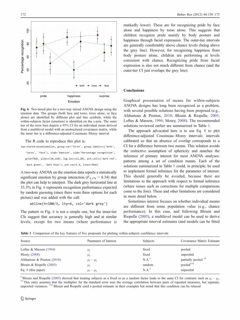
The R code to reproduce this plot is:

A two-way ANOVA on the emotion data reports a statisticallysignificant emotion by group interaction (F4,174 = 8.34) thatthe plot can help to interpret. The dark grey horizontal line at33.3% in Fig. 6 represents recognition performance expectedby random guessing (since there were three options for eachpicture) and was added with the call:

The pattern in Fig. 6 is not a simple one, but the inner-tierCIs suggest that accuracy is generally high and at similarlevels, except for two means (where performance is

markedly lower). These are for recognizing pride by facealone and happiness by torso alone. This suggests thatchildren recognize pride mainly by body posture andhappiness through facial expression. The outer-tier intervalsare generally comfortably above chance levels (being abovethe grey line). However, for recognizing happiness frombody posture alone, children are performing at levelsconsistent with chance. Recognizing pride from facialexpression is also not much different from chance (and theouter-tier CI just overlaps the grey line).

Conclusions

Graphical presentation of means for within-subjectsANOVA designs has long been recognized as a problem,with several possible solutions having been proposed (e.g.,Afshartous & Preston, 2010; Blouin & Riopelle, 2005;Loftus & Masson, 1994; Morey, 2008). The recommendedsolutions reviewed earlier are summarized in Table 1.

The approach advocated here is to use Eq. 8 to plotdifference-adjusted Cousineau–Morey intervals: intervalscalibrated so that an absence of overlap corresponds to aCI for a difference between two means. This solution avoidsthe restrictive assumption of sphericity and matches theinference of primary interest for most ANOVA analyses:patterns among a set of condition means. Each of thesolutions summarized in Table 1 could, in principle, be usedto implement formal inference for the parameter of interest.This should generally be avoided, because there arelimitations to the approach with respect to formal inference(where issues such as corrections for multiple comparisonscome to the fore). These and other limitations are consideredin more detail below.

Sometimes interest focuses on whether individual meansare different from some population value (e.g., chanceperformance). In this case, and following Blouin andRiopelle (2005), a multilevel model can be used to derivethe appropriate interval estimates (and models can be fitted

2040

6080

100

Emotion

Per

cent

age

reco

gniti

on

pride happiness surprise

both torso face

Fig. 6 Two-tiered plot for a two-way mixed ANOVA design using theemotion data. The groups (both face and torso, torso alone, or facealone) are identified by different plot and line symbols, while thewithin-subjects factor (emotion) is identified on the x-axis. The outertier of the error bars depicts a 95% CI for an individual mean derivedfrom a multilevel model with an unstructured covariance matrix, whilethe inner tier is a difference-adjusted Cousineau–Morey interval

Table 1 Comparison of the key features of five proposals for plotting within-subjects confidence intervals

Source Parameter of Interest Subjects Covariance Matrix Estimate

Loftus & Masson (1994) μj fixed pooled

Morey (2008) μj fixed unpooled

Afshartous & Preston (2010) μi – μj N.A.† partially pooled ††

Blouin & Riopelle (2005) μj random pooled†††

Eq. 8 (this paper) μi – μj N.A.† unpooled

†Blouin and Riopelle (2005) showed that treating subjects as a fixed or as a random factor leads to the same CI for contrasts such as μi – μj.††This entry assumes that the multiplier for the standard error uses the average correlation between pairs of repeated measures, but separate,unpooled variances. †††Blouin and Riopelle used a pooled estimate in their examples but noted that this condition can be relaxed

172 Behav Res (2012) 44:158–175

that relax the sphericity assumption or cope with imbal-ance). In many cases, both types of inference are of interest,and two-tiered CIs can be plotted. In a two-tiered plot, theouter tier depicts the CI for an individual mean and theinner tier supports inferences about differences betweenmeans. For plotting large numbers of means or otherstatistics, a Goldstein–Healy plot is a convenient alternative(Afshartous & Preston, 2010; Goldstein & Healy, 1995).

A practical obstacle to graphical presentation of meansis that few of the options are implemented in widelyavailable statistics software. I have provided R functionsthat compute CIs and generate both one-tiered and two-tiered plots for the Loftus–Masson, Cousineau–Morey,and multilevel approaches reviewed here. The initialfocus is on intervals for a one-way ANOVA design, but itis possible to modify these functions for more complexdesigns (and this is illustrated for a two-way mixedANOVA).

Potential limitations There are several potential limita-tions of the approach advocated here. First, emphasis ison informal inference about means or patterns of means.The interval estimates proposed here will be reasonablyaccurate for most within-subjects ANOVA designs, butare intended chiefly as an aid to the exploration andinterpretation of data. Thus, they may compliment formalinference, but are not intended to mimic null-hypothesissignificance tests.

Even so, informal inference is more than sufficient toresolve many research questions—notably where the effectsare very salient in a graphical display. This suggests thatformal inference should be reserved to test hypotheses thatrelate to patterns that are not easily detected by eye, or toquantify the degree of support for a particularly importanthypothesis. In the context of ANOVA, such hypotheses are nottypically addressed by the omnibus test of an effect, but byfocused contrasts (see, e.g., Loftus, 2001; Rosenthal, Rosnow,& Rubin, 2000).16 Furthermore, formal inference need nottake the form of a null-hypothesis significance test. Rouder,Speckman, Sun, Morey, and Iverson (2009) recommend CIsfor reporting data but advocate Bayes factors for formalinference. Dienes (2008) describes approaches for Bayesianand likelihood-based inference for contrasts among means

and provides MATLAB code to implement them.17 Contrastsare particularly useful for testing hypotheses about complexinteraction effects (Abelson & Prentice, 1997). Thus, thelimitations of graphical methods for inference may, paradox-ically, be an advantage. As noted in the introduction,significance tests tend to be overused, and those tests notrelating to the main hypotheses of interest can often bereplaced by a graph with appropriate interval estimates.Formal inference can then be reserved for tests of a smallnumber of important hypotheses.

A second limitation is that all of the approaches discussedhere make distributional assumptions that may not hold inpractice. Where the errors of the statistical model are not atleast approximately normal—and particularly where theyfollow heavy-tailed or highly skewed distributions—intervalestimates based on the z or t distribution may not providegood approximations (see, e.g., Afshartous & Preston, 2010).For the Loftus–Masson and Cousineau–Morey approaches, itis possible to apply bootstrap solutions. Wright (2007)provides R functions for bootstrap versions of the Loftus–Masson intervals for one-way ANOVA. For more complexdesigns, it is advisable to apply a bespoke solution. The bestapproach may be to bootstrap trimmed means or medians(rather than means), and the adequacy of the bootstrapsimulations in each case needs to be checked (see Wilcox &Keselman, 2003). Similar reservations arise for complexmultilevel models. However, the equivalence of multilevelmodels with balanced designs to within-subjects ANOVAmodels (at least when restricted maximum likelihoodestimation is used and compound symmetry assumed)suggests that CIs will be sufficiently accurate for the rangeof models implemented here. This may no longer be true forvery unbalanced designs or where the distributional assump-tions of ANOVA are severely violated. One alternative is toobtain the highest posterior density (HPD) intervals fromMarkov chain Monte Carlo simulations (see, e.g., Baayen,Davidson, & Bates, 2008). In addition, if bootstrapping orother approaches are required for the CIs, the conventionalANOVA model may be unsuitable, and other approachesshould be considered. In short, if a within-subjects ANOVA isconsidered suitable in the first place, the proposed solutionsimplemented here should suffice for informal inference.

The final limitation is that I have not explicitlyconsidered the issue of multiple testing. Correcting formultiple testing is a difficult problem for informal infer-ence. As a large number of inferences can be drawn, and asdifferent people will be interested in different questions, itmay not be appropriate to determine any correction inadvance. For graphical presentation of means, it is moreappropriate to report uncorrected CIs and take account ofmultiple testing in other ways. For example, with J = 5

16 Any ANOVA contrast can be viewed as a difference between twomeans (constructed from weighted linear combinations of a set ofsample means). It is therefore relatively straightforward to plot a CIfor a contrast using conventional methods (though it is generally morehelpful to plot the set of unweighted means, as advocated here). If aplot of the contrast itself is required, it is probably better to plot a CIof the weighted difference itself rather than plot the weighted meansseparately. In addition, it is important to rescale the contrast weights sothat their absolute sum is 2, or else the difference will no longer be onthe same scale as the original means (see Kirk, 1995, p. 114). 17 For R code, see Baguley and Kaye (2010).

Behav Res (2012) 44:158–175 173

means, there are J J � 1ð Þ=2 ¼ 10 possible pairwisecomparisons. This implies that one pair of appropriatelyadjusted 95% CIs would be expected not to overlap just bychance. Where the number of inferences to be drawn isknown in advance, it is possible to make a Bonferroni-stylecorrection by altering the confidence level (e.g., for fivetests, a 99% CI is a Bonferroni-adjusted 95% CI). Thedrawback of this approach is that corrections for multipletesting suitable for plotting tend to be very conservative. Ifmultiple corrections are critical, it is best to supplementgraphical presentation with formal a priori or post hocinference using a procedure that also controls Type I errorrates in a strong fashion.18 There are also more formaltreatments of the multiple-comparison problem in relationto a Goldstein–Healy plot (see Afshartous & Preston, 2010;Afshartous & Wolf, 2007).

Summary It is possible to offer a solution to plottingwithin-subjects CIs that is both accurate and robust toviolations of sphericity. The intervals themselves can becalculated and plotted in R with the functions providedhere. These interval estimates are suitable for exploratoryanalyses and informal inference when reporting datafrom classical ANOVA designs, and they are designed tosupport graphical inference about the pattern of meansacross conditions. When both types of inference are ofinterest, they can be displayed together as a two-tieredCI.

Author note The author thanks Andy Fugard, Ken Kelley, GregoryFrancis, and two anonymous reviewers for providing constructivecomments on previous drafts of the manuscript.

Appendix

This code tricks SPSS into plotting 95% confidenceintervals for the Loftus and Masson (1994) free recall datawith the Cousineau–Morey approach. The first set ofcommands computes the required confidence level toobtain a 95% CI, using the normalized scores for n perlevel = 10 and J = 3 levels. To adjust any of these values,just edit the appropriate value of the input (0.95, 3, or 10).

This should return the target confidence level (97.83%) as avariable in a new data view window and return the value tothe output window (along with the inputs).

At this point, open or make active the SPSS data file. The next set of commands calculates the

normalized data (and is adapted from Cousineau, 2005).

To obtain the 95% Cousineau–Morey intervals, either usethe one-sample T-TEST procedure or plot the CIs using97.83% as the nominal confidence level.

These in t e rva l s ma tch those o f the ca l lto the

R function provided in the supplementary materials toabout three decimal places.

References

Abelson, R. P. (1995). Statistics as principled argument. Hillsdale:Erlbaum.

18 Multiple testing can also be addressed by switching to Bayesian orlikelihood-based methods. However, there is some disagreement aboutwhether multiple testing is a problem outside of frequentist statistics(for a brief discussion, see Dienes, 2008).

174 Behav Res (2012) 44:158–175

Abelson, R. P., & Prentice, D. A. (1997). Contrast tests of interactionhypotheses. Psychological Methods, 2, 315–328.

Afshartous, D., & Preston, R. A. (2010). Confidence intervals fordependent data: Equating nonoverlap with statistical signifi-cance. Computational Statistics and Data Analysis, 54, 2296–2305.

Afshartous, D., & Wolf, M. (2007). Avoiding data snooping inmultilevel and mixed effects models. Journal of the RoyalStatistical Society: Series A, 170, 1035–1059.

American Psychological Association. (2010). Publication manual ofthe American Psychological Association (6th ed.). Washington:Author.

Baayen, R. H., Davidson, D. J., & Bates, D. M. (2008). Mixed-effectsmodeling with crossed random effects for subjects and items.Journal of Memory and Language, 59, 390–412.

Baguley, T. (2009). Standardized or simple effect size: What should bereported? British Journal of Psychology, 100, 603–617.

Baguley, T., & Kaye, W. S. (2010). Review of Understandingpsychology as a science: An introduction to scientific andstatistical inference. British Journal of Mathematical andStatistical Psychology, 63, 695–698.

Bakeman, R., & McArthur, D. (1996). Picturing repeated measures:Comments on Loftus, Morrison, and others. Behavior ResearchMethods, Instruments, & Computers, 28, 584–589.

Belia, S., Fidler, F., Williams, J., & Cumming, G. (2005). Researchersmisunderstand confidence intervals and standard error bars.Psychological Methods, 10, 389–396.

Blouin, D. C., & Riopelle, A. J. (2005). On confidence intervalsfor within-subject designs. Psychological Methods, 10, 397–412.

Cleveland, W. S. (1985). The elements of graphing data. New York:Chapman & Hall.

Cousineau, D. (2005). Confidence intervals in within- subject designs:A simpler solution to Loftus and Masson’s method. Tutorials inQuantitative Methods for Psychology, 1, 42–45.

Cumming, G., & Finch, S. (2005). Inference by eye: Confidenceintervals, and how to read pictures of data. American Psychologist,60, 170–180.

Dienes, Z. (2008). Understanding psychology as a science: Anintroduction to scientific and statistical inference. Basingstoke:Palgrave Macmillan.

Fidler, F., & Loftus, G. (2009). Why figures with error bars shouldreplace p values: Some conceptual arguments and empiricaldemonstrations. Zeitschrift für Psychologie, 217, 27–37.

Goldstein, H., & Healy, M. J. R. (1995). MJR: The graphicalpresentation of a collection of means. Journal of the RoyalStatistical Society: Series A, 158, 175–177.

Hollands, J. G., & Jarmasz, J. (2010). Revisiting confidence intervals forrepeated-measures designs. Psychonomic Bulletin & Review, 17,135–138.

Hox, J. J. (2010). Multilevel analysis: Techniques and applications(2nd ed.). Mahwah: Erlbaum.

Jarmasz, J., & Hollands, J. G. (2009). Using confidence intervals inrepeated-measures designs: The number of observationsprinciple. Canadian Journal of Experimental Psychology, 63,124–138.

Kelley, K., Maxwell, S. E., & Rausch, J. R. (2003). Obtaining poweror obtaining precision: Delineating methods of sample sizeplanning. Evaluation & the Health Professions, 26, 258–287.

Keselman, H. J., Algina, J., & Kowalchuk, R. K. (2001). The analysisof repeated measures designs: A review. British Journal ofMathematical and Statistical Psychology, 54, 1–20.

Kirk, R. E. (1995). Experimental design (3rd ed.). Belmont: Brooks/Cole.

Loftus, G. R. (2001). Analysis, interpretation, and visual presentationof experimental data. In J. Wixted & H. Pashler (Eds.), Stevens’handbook of experimental psychology: Vol. 4. Methodology inexperimental psychology (3rd ed., pp. 339–390). New York:Wiley.

Loftus, G. R., & Masson, M. E. J. (1994). Using confidence intervalsin within-subject designs. Psychonomic Bulletin & Review, 1,476–490.

Masson, M. E. J., & Loftus, G. R. (2003). Using confidence intervalsfor graphically based data interpretation. Canadian Journal ofExperimental Psychology, 57, 203–220.

Mitzel, H. C., & Games, P. A. (1981). Circularity and multiplecomparisons in repeated measures designs. British Journal ofMathematical and Statistical Psychology, 34, 253–259.

Morey, R. D. (2008). Tutorials in Quantitative Methods for Psychology,4, 61–64.

Moses, L. E. (1987). Graphical methods in statistical analysis. AnnualReview of Public Health, 8, 309–353.

Pinheiro, J., Bates, D., DebRoy, S., Sarkar, D., & the R Core Team(2009). nlme: Linear and nonlinear mixed effects models. Rpackage version 3.1-92.

R Development Core Team. (2009). R: A language and environmentfor statistical computing. Vienna: R Foundation for StatisticalComputing. Available at www.R-project.org.

Rosenthal, R., Rosnow, R. L., & Rubin, D. B. (2000). Contrasts andcorrelations in behavioral research. New York: CambridgeUniversity Press.

Rouder, J. N., Speckman, P. L., Sun, D., Morey, R. D., &Iverson, G. (2009). Bayesian t tests for accepting andrejecting the null hypothesis. Psychonomic Bulletin & Review,16, 225–237.

Rozeboom, W. W. (1960). The fallacy of the null-hypothesissignificance test. Psychological Bulletin, 57, 416–428.

Schenker, N., & Gentleman, J. F. (2001). On judging the significanceof differences by examining the overlap between confidenceintervals. The American Statistician, 55, 182–186.

Searle, S. R., Casella, G., & McCulloch, C. E. (1992). Variancecomponents. New York: Wiley.

Uppal, A. (2006). Can children effectively recognize pride frombody posture or facial expression? Unpublished BSc. psychol-ogy research project. Nottingham Trent University, Nottingham,U.K.

Warnes, G. R., Bolker, B., Lumley, T., & Johnson, R. C. (2009).gmodels: Various R programming tools 1397 for model fitting. Rpackage version 2.15.0. Available at http://CRAN.R-project.org/package=gmodels.

Wilcox, R. R., & Keselman, H. J. (2003). Modern robust data analysismethods: Measures of central tendency. Psychological Methods,8, 254–274.

Wilkinson, L., & the Task Force on Statistical Inference. (1999).Statistical methods in psychology journals: Guidelines andexplanations. American Psychologist, 54, 594–604.

Wright, D. B. (2007). Graphingwithin subject confidence intervals (WSCI)using SPSS and S-Plus. Behavior Research Methods, 39, 82–85.

Behav Res (2012) 44:158–175 175