Calculating potential carbon losses and savings from wind farms on Scottish peatlands Technical Note – Version 2.10.0.

Wind farms and carbon savings on peatlands

This note presents a revised methodology to calculate carbon emission savings associated with wind farm developments on Scottish peatlands. It supports the use of the Scottish Government’s carbon calculator (http://informatics.sepa.org.uk/CarbonCalculator/). It is assumed in this note that good management practice is followed, as outlined by the Scottish Executive (2006), to avoid catastrophic losses of carbon, such as by peat landslides.

Summary

Large scale wind farm development proposals in Scotland have raised concerns about the reliability of methods used to calculate any associated carbon savings, as compared to power derived from fossil-fuel and other more conventional sources of power generation. This is largely due to the potential siting of wind farms on peatlands which represent large stores of terrestrial carbon. Scottish Government policy is to deliver renewable energy without environmental harm and to deliver biodiversity objectives, including the conservation of designated wildlife sites and important habitats such as peatlands. The implication for carbon emissions of developing a wind farm is therefore just one factor that should be included in the consideration of such a proposed development. This Technical Note provides a revised methodology to explore potential carbon emission savings and losses associated with a wind farm development in forestry or on peatland. The total savings of carbon emissions from a wind farm are estimated with respect to emissions from different sources of power generation. Losses of carbon are accounted for due to production, transportation, erection, operation and dismantling of the wind farm, backup power generation, loss of carbon-fixing potential of peatland, loss of carbon stored in peatland, carbon saving due to improvement of habitat and loss of carbon-fixing potential as a result of forestry clearance.

Contents Glossary ..................................................................................................................................................................... 3 Introduction ................................................................................................................................................................. 5 Background ................................................................................................................................................................ 6 Carbon emission savings ............................................................................................................................................ 6 Carbon emission savings from wind farms .................................................................................................................. 7 Loss of carbon due to production, transportation, erection, operation and decommissioning of wind farm .................. 8 Loss of carbon due to backup power generation ......................................................................................................... 9 Change in carbon dynamics of peatlands ................................................................................................................. 10 Loss of carbon fixing potential of peatlands............................................................................................................... 10 Changes in carbon stored in peatlands ..................................................................................................................... 11

Loss of carbon from removed peat ...................................................................................................................... 11 Loss of carbon from drained peat ........................................................................................................................ 12

Estimation of volume of peat affected by drainage ......................................................................................... 12 Loss of carbon from drained peat if the site is not restored after decommissioning ......................................... 13 Loss of carbon from drained peat if the site is restored after decommissioning............................................... 13

Loss of carbon dioxide due to leaching of dissolved and particulate organic carbon ............................................ 16 Loss of carbon due to peatslide ........................................................................................................................... 16

Changes of carbon due to forestry clearance ............................................................................................................ 16 Simple method for calculating carbon sequestered in forestry ............................................................................. 17 Detailed method for calculating carbon sequestered in forestry ........................................................................... 17

Environmental modifier used in simplified 3PGN ............................................................................................ 17 Light Interception ............................................................................................................................................ 18 Primary productivity .................................................................................................................................... 19 Cleared Forest Floor Emissions ..................................................................................................................... 19 Emissions from harvesting operations ............................................................................................................ 19 Savings from use of felled forestry as biofuel ................................................................................................. 20 Savings from use of replanted forestry as a biofuel ........................................................................................ 20 Total carbon loss associated with forest management .................................................................................... 21

Impacts of forestry management on windfarm carbon emission savings ................................................................... 21 Capacity factor .................................................................................................................................................... 21 Windspeed ratio .................................................................................................................................................. 22

Relative windspeed ........................................................................................................................................ 22 Relative upwind windspeed ............................................................................................................................ 22 Relative downwind windspeed........................................................................................................................ 22

Carbon dioxide saving due to improvement of peatland habitat ................................................................................ 23 Calculation of payback time for the example case-study wind farm ........................................................................... 24 References ............................................................................................................................................................... 24

Glossary

Access track – Roadways constructed as part of the windfarm development to provide access of heavy machinery to turbines. Acid bog – a wetland fed primarily by rainwater and often inhabited by sphagnum moss, thus making it acidic (Stoneman & Brooks, 1997). Auger – tool used to obtain a disturbed soil sample at or near the surface of the soil for further analysis . Backup - the extra electricity generation capacity required to maintain electricity supply during times of low wind generation Basin bog – a raised bog that forms through infilling of a basin by fen peat, eventually forming into a bog peat (IUCN, 2014). Blanket bog – peat formations, mainly found in the UK uplands, that cover the entire landscape; generally thinner than lowland peats (IUCN, 2014). Bog – wetland that is waterlogged only by direct rainfall (IUCN, 2014). Capacity factor - The capacity factor of a windfarm is the proportion of energy produced during a given period with respect to the energy that would have been produced had the wind farm been running continually at maximum output. Note that the term ‘load factor’ can be used interchangeably with Capacity Factor. Carbon sequestration – Long term accumulation of carbon. Chipping – Removal of commercial crop (e.g. lodgepole pine) or young low yielding conifers, but leaving a clean bog surface. Trees are felled manually by chainsaw and fed into a tractor-powered chipper by an excavator fitted with a tree grab. Commercial removal of conifers – Aim to remove commercial crop (e.g. lodgepole pine). For example, the trees are cut by a harvester and removed to roads/access tracks by a forwarder running on brash mats made of felled trees. Decommissioning of the wind farm – De-energising and removing wind farm infrastructure (Welstead et al., 2013). Deep peat - Soil with a surface organic horizon > 1.0 m deep, as defined by JNCC report 445 (SG, 2014). Depthing rods – peat probes used to measure total peat depth (Scottish Government, 2016). Dipwells – Plastic tubing (usually 5 cm diameter 1.0 m to 1.5 m in length), perforated with holes of at least 5 mm diameter, or slits of similar dimension, along its entire length (except the top 100 mm). The pipe is usually covered with a sleeve of woven material to exclude silt entry. Dipwells are used to measure water table depth. Dry soil bulk density – The density of weight of a specified volume of peat when dried. ECOSSE – A model of nitrogen and carbon turnover in soils developed by the University of Aberdeen under funding from the Scottish Government (Smith et al., 2010). Emission factor – The amount of carbon dioxide emitted per MWh of generated electricity. Emissions from construction, operation and civil works of a windfarm. – Emissions from the full life cycle of a wind farm, including CO2 emissions that occur during production,

transportation, erection, operation, dismantling and removal of turbines, foundations and the transmission grid from the existing electricity grid. Erosion gullies - large ditches that can be up to 10 m wide. Water flow rate in the gully can be substantial, which causes the significant deep cutting action and removal of soil by erosion. Extent of drainage – the distance from a drainage feature (e.g. a ditch) over which impacts of drainage on the water content/position of water tablein soil can be measured. Felling to waste of young/low yielding conifers – Aims to remove trees that have grown poorly due to wet/poor conditions. Manual felling is usually done by chainsaw with trees either left on site or removed by windrowing (rolling the trees in a single row, e.g. in the drainage ditches). Fen - a type of wetland fed by surface and/or groundwater (McBride et al., 2011). Fixation of carbon by plants – Conversion of carbon dioxide to organic compounds by plants. Fossil Fuel-Mix – The annual average mix of fuels used to produce electricity for British (GB) electricity grid excluding nuclear and renewables. Floating road – Road constructed on the existing ground surface normally with one or two layers of geogrids interlocked with crushed rock aggregates to build up a strong mechanically stabilised layer. Aims to avoid excessive drainage or removal of peats (SNH, 2015). Grazing reduction / enclosure - Aims to 1. Prevent excessive grazing, 2. Allow recolonisation of bare peat, 3. Reduce trampling. Stocking is reduced to ≤0.5 sheep/ha and/or removal of winter grazing and/or fencing of highly sensitive areas. Grid mix – The annual average mix of fuels used to produce electricity for the (GB) electricity grid (including nuclear and renewables). Grip blocking – Aims to block artificial drainage ditches and facilitate rewetting. Blocking of drainage ditches is done using peat turfs, plastic piles, wooden dams, heather bales, straw bales, stones, etc. Avoid blocking during very wet period (e.g. snowmelt) and block prior to the beginning of the growing season. May be better to start damming upslope and then work down. Minimise site disturbance by not leaving bare peat or exposed mineral soil, and creating escape routes for water from dams. Ground penetrating radar - a geophysical surveying method that uses radar pulses to image subsurface structures. Gully Blocking - Aims to 1. Raise water table in flat areas, 2. Limit directional flow and reduce flow rate in gullies, 3. Prevent widening and deepening of gullies. Dams are built across the gullies at intervals of ~15 m using various materials such as peat, wood, stones, bales, vegetation, wool or plastic piling. Plastic piling is most effective for deep gullies. Should target slopes of <10% and carefully plan blocking considering slope, surrounding topography and wetness and vegetation. Improvement of carbon sequestration at the site - Actions taken to increase carbon sequestration in areas of the site that may have been previous degraded, drained or disturbed. Actions may include removal of drains, replacement of peat and habitat restoration. Introduction of Heather - Aims to stabilize small areas of bare peat surface. Heather brash is cut from nearby area and spread with a 1:2 ratio over degraded area or heather seeds are sown. IPCC default methodology - the internationally accepted standard for calculating emissions of carbon dioxide (IPCC, 1997).

Lifetime of windfarm – The time from commissioning to decommissioning of the wind farm. Load factor – another term for “capacity factor” (see above). Nurse crop and geotextile - Aims to stabilize peat surface on highly eroded areas. Sites are seeded with a nurse seed mix (e.g. Deschampsia flexuosa, Agrostis castellana, Festuca ovina, Lolium perenne) following the application of geotextile on peat surface. Peat – organic material derived from dead plants, accumulated under wet/waterlogged (mainly anaerobic) conditions. This material can be characterised as fibrous or amorphous, depending on the decomposition stage of the organic material. For the purpose of the Carbon Calculator, this term is used to refer to all peaty and other highly organic soils. The carbon content of peats is between 49% and 62% (Birnie et al., 1991). Peat depth – Depth from surface to mineral layer of peat or highly organic soil. Peat soil - a soil with a surface organic layer greater than 0.5m deep which has an organic matter content of more than 60%. Peaty (or organo-mineral) soil - a soil with a surface organic layer less than 0.5m deep, as defined by JNCC report 445. Examples include peaty gleys and peaty podzols. Rated capacity – For a windfarm this is the maximum power output that can be produced by the wind turbine or wind farm. For a conventional power station it is the ratio of useful electrical energy output to the total energy input in the form of fuel. Topographic survey – identification and mapping the contours of the ground surface and the soil and mineral layers below the ground Water table depth – the upper boundary of the saturated zone within the soil Wind farm site - the area of the proposed siting of turbines, access tracks, drainage infrastructure, including adequate additional area to accommodate revised positioning of the turbines. For the purposes of calculating average depth of peat, extent of drainage and water table depth at the site, only the area of peat where turbines will be located should be included. Yield class of forestry – Mean annual increment in yield (measured in m3 ha-1).

Introduction

1. The 2011 renewable energy policy of the Scottish Government (SG) has a target of renewable sources generating the equivalent of 100% of annual electricity demand by 2020, with an interim target of 50% by 2015 (Scottish Government, 2015).

2. Scottish Natural Heritage (SNH) stresses the value of renewable sources of electricity generation in tackling climate change and provides advice on the siting of renewable energy installations to ensure that the technology is best matched to the potential offered by a location to minimise adverse impacts on the natural heritage (SNH, 2007, pages 23, 36).

3. Any attempt to meet a 100% target relying substantially on onshore wind could result in increasingly difficult trade-offs with natural heritage interests. One argument that is sometimes mooted against wind farm development is based on the likely overall carbon savings associated with developments in forestry or on peatland.

4. SNH published a Technical Guidance Note in 2003 for calculating carbon ‘payback’ times for wind farms. The 2003 guidance adopted a relatively simple approach towards impacts on peatland hydrology and stability. This note represents a more comprehensive approach towards these issues.

Background

5. Organic soils are abundant in Scotland, containing 2735 Mt carbon. Scotland contains 48% of the soil carbon stocks of the UK (Bradley et al., 2005). Depending on land management, organic soils can either act as carbon sinks or as carbon sources. Soils in Scotland act as a carbon sink, absorbing 1.26 Mt CO2-C more carbon dioxide than they release due to the impacts of changes in land use, including forestry (Key Scottish Environment Statistics, 2007). Estimates of emissions and removals from this sector are particularly uncertain as they depend on assumptions made on the rate of loss or gain of carbon in Scotland's carbon rich soils (Key Scottish Environment Statistics, 2007). Land use change and climate change can cause emissions of GHGs; for example, land use change on organic soils is estimated to be responsible for 15% of Scotland’s total greenhouse gas emissions.

6. Large scale wind farm development on organic soils (largely peats) has raised concerns about the reliability of methods used to calculate the time taken for these facilities to reduce greenhouse gas emissions. This note provides a revised methodology to calculate carbon emission savings and the carbon dioxide payback time of a wind farm development, and explore the potential implications under different scenarios of development and assumptions about the site. It discusses the potential carbon savings and carbon costs associated with wind farm developments as follows:

i. carbon emission savings (based on emissions from different power sources)

ii. loss of carbon due to production, transportation, erection, operation and decommissioning of the wind farm

iii. loss of carbon from backup power generation

iv. loss of carbon-fixing potential of peatland

v. loss and/or saving of carbon stored in peatland (by peat removal or changes in drainage)

vi. carbon saving due to improvement of habitat

vii. loss and/or saving of carbon-fixing potential as a result of forestry clearance.

Carbon emission savings

7. Emissions may be quoted in terms of tonnes of CO2 or tonnes of C. The conversion figures are: 1 tonne C = 3.667 tCO2

1 tCO2 = 0.27 tC

8. Authoritative figures for calculating emissions from various sources, including power stations, are given https://www.gov.uk/government/collections/government-conversion-factors-for-company-reporting Worked examples, including one for the carbon saved by generating electricity from wind energy as opposed to the conventional mix (including fossil fuel sources), are given by The Carbon Trust ( www.carbontrust.co.uk ).

9. Carbon dioxide emissions from energy production depend on the fuel used (Table 1).

Fuel Carbon dioxide released

during combustion

(tCO2 MWh-1)

Natural Gas 0.185

Gas/Diesel Oil 0.250

Petrol 0.240

Fuel Oil 0.267

Burning Oil 0.245

Coal 0.329

Coking Coal 0.332

LPG 0.214

Fuel Carbon dioxide released

during combustion

(tCO2 MWh-1)

Other Petroleum Gas 0.206

Aviation Spirit 0.238

Aviation Turbine Fuel 0.245

Naphtha 0.237

Lubricants 0.250

Petroleum Coke 0.343

Refinery Miscellaneous 0.246

Renewables 0.000

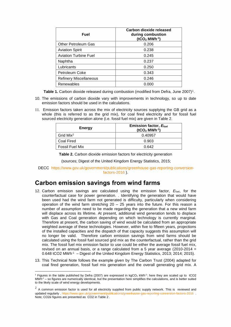
Table 1. Carbon dioxide released during combustion (modified from Defra, June 2007)1.

10. The emissions of carbon dioxide vary with improvements in technology, so up to date emission factors should be used in the calculations.

11. Emission factors taken across the mix of electricity sources supplying the GB grid as a whole (this is referred to as the grid mix), for coal fired electricity and for fossil fuel sourced electricity generation alone (i.e. fossil fuel mix) are given in Table 2.

Energy Emission factor, Efuel

(tCO2 MWh-1)

Grid Mix2 0.40957

Coal Fired 0.903

Fossil Fuel Mix 0.642

Table 2. Carbon dioxide emission factors for electricity generation

(sources; Digest of the United Kingdom Energy Statistics, 2015;

DECC https://www.gov.uk/government/publications/greenhouse-gas-reporting-conversion-factors-2016 ).

Carbon emission savings from wind farms

12. Carbon emission savings are calculated using the emission factor, Efuel, for the counterfactual case for power generation. . Identifying the generation that would have been used had the wind farm not generated is difficulty, particularly when considering operation of the wind farm stretching 20 – 25 years into the future. For this reason a number of assumption need to be made regarding the generation that a new wind farm will displace across its lifetime. At present, additional wind generation tends to displace with Gas and Coal generation depending on which technology is currently marginal. Therefore at present, the carbon saving of wind would be calculated from an appropriate weighted average of these technologies. However, within five to fifteen years, projections of the installed capacities and the dispatch of that capacity suggests this assumption will no longer be valid. Therefore carbon emission savings from wind farms should be calculated using the fossil fuel sourced grid mix as the counterfactual, rather than the grid mix. The fossil fuel mix emission factor to use could be either the average fossil fuel mix, revised on an annual basis, or a range calculated from a 5 year average (2010-2014 = 0.648 tCO2 MWh-1 – Digest of the United Kingdom Energy Statistics, 2013; 2014; 2015).

13. This Technical Note follows the example given by The Carbon Trust (2004) adapted for coal fired generation, fossil fuel mix generation and the overall generating grid mix. A

1 Figures in the table published by Defra (2007) are expressed in kgCO2 kWh-1: here they are scaled up to tCO2 MWh-1 – so figures are numerically identical, but the presentation here simplifies the calculations, and is better suited to the likely scale of wind energy developments. 2 A common emission factor is used for all electricity supplied from public supply network. This is reviewed and

updated regularly . https://www.gov.uk/government/publications/greenhouse-gas-reporting-conversion-factors-2016 . Note; CO2e figures are presented as CO2 in Table 2 .

renewable energy development will have a maximum potential to ‘save’ carbon emissions if it is substituting coal fired generation. However, in most circumstances it is not possible to define the electricity source for which a renewable electricity project will substitute. The calculations in this Note include options for three sets of figures i.e. substitution for coal generated electricity, substitution for fossil fuel generated electricity and substitution for grid mix.

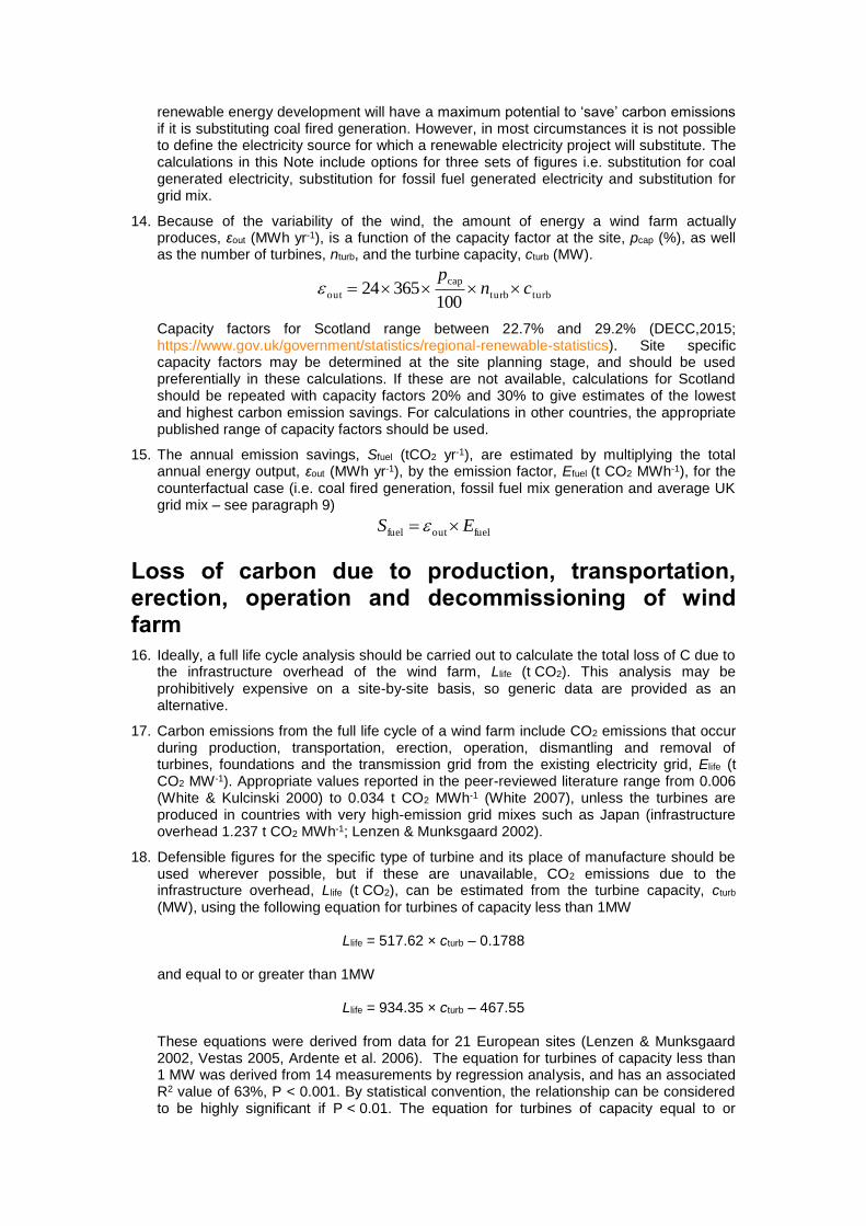
14. Because of the variability of the wind, the amount of energy a wind farm actually produces, εout (MWh yr-1), is a function of the capacity factor at the site, pcap (%), as well as the number of turbines, nturb, and the turbine capacity, cturb (MW).

turbturb

cap

out100

36524 cnp

Capacity factors for Scotland range between 22.7% and 29.2% (DECC,2015; https://www.gov.uk/government/statistics/regional-renewable-statistics). Site specific capacity factors may be determined at the site planning stage, and should be used preferentially in these calculations. If these are not available, calculations for Scotland should be repeated with capacity factors 20% and 30% to give estimates of the lowest and highest carbon emission savings. For calculations in other countries, the appropriate published range of capacity factors should be used.

15. The annual emission savings, Sfuel (tCO2 yr-1), are estimated by multiplying the total annual energy output, εout (MWh yr-1), by the emission factor, Efuel (t CO2 MWh-1), for the counterfactual case (i.e. coal fired generation, fossil fuel mix generation and average UK grid mix – see paragraph 9)

fueloutfuel ES

Loss of carbon due to production, transportation, erection, operation and decommissioning of wind farm

16. Ideally, a full life cycle analysis should be carried out to calculate the total loss of C due to the infrastructure overhead of the wind farm, Llife (t CO2). This analysis may be prohibitively expensive on a site-by-site basis, so generic data are provided as an alternative.

17. Carbon emissions from the full life cycle of a wind farm include CO2 emissions that occur during production, transportation, erection, operation, dismantling and removal of turbines, foundations and the transmission grid from the existing electricity grid, Elife (t CO2 MW-1). Appropriate values reported in the peer-reviewed literature range from 0.006 (White & Kulcinski 2000) to 0.034 t CO2 MWh-1 (White 2007), unless the turbines are produced in countries with very high-emission grid mixes such as Japan (infrastructure overhead 1.237 t CO2 MWh-1; Lenzen & Munksgaard 2002).

18. Defensible figures for the specific type of turbine and its place of manufacture should be used wherever possible, but if these are unavailable, CO2 emissions due to the infrastructure overhead, Llife (t CO2), can be estimated from the turbine capacity, cturb (MW), using the following equation for turbines of capacity less than 1MW

Llife = 517.62 × cturb – 0.1788

and equal to or greater than 1MW

Llife = 934.35 × cturb – 467.55

These equations were derived from data for 21 European sites (Lenzen & Munksgaard 2002, Vestas 2005, Ardente et al. 2006). The equation for turbines of capacity less than 1 MW was derived from 14 measurements by regression analysis, and has an associated R2 value of 63%, P < 0.001. By statistical convention, the relationship can be considered to be highly significant if P < 0.01. The equation for turbines of capacity equal to or

greater than 1 MW was derived similarly from seven measurements; the associated R2 value is 85%, P < 0.01, and thus again highly significant.

Emissions due to use of concrete in construction, Lconcrete (t CO2), are calculated from the entered volume of concrete used, Vconcrete (m3), and the emission factor for reinforced foundations, Econcrete (t CO2 m-3 concrete), as

𝐿concrete = 𝑉concrete × 𝐸concrete

The value for Econcrete is assumed to be 0.316 t CO2 m-3 concrete ( The Concrete centre, 2013)

Loss of carbon due to backup power generation

19. Because wind generated electricity is inherently variable, accompanying backup power is required to stabilise the supply to the consumer. The extra capacity needed for backup power generation, pback, is currently estimated to be 5% of the rated capacity of the wind plant if wind power contributes more than 20% to the national grid (Dale et al., 2004)

a. The unpredictable nature of wind generation, even a few hours before delivery, requires that backup generation is availability from dispatchable plant to provide security of supply. National Grid as GB System Operator (SO) manages the uncertainty in wind power availability along with a number of other important uncertainties in the run up to operation. In particular, uncertainty around the level of demand and uncertainty over the availability of conventional generation must be included (conventional generation is uncertain as a fault may make it unavailable right up to operation). Where the penetration of wind across the GB system is relatively small, the impact of demand and conventional generation availability will dominate. As wind penetration increases this situation changes and the SO must consider forecasts of wind output when deciding on what levels of reserve to hold. A further complication is that the level and type of back-up availability changes as the time until operation reduces, a result of the fact that wind availability is likely to be more certain one hour ahead of operation than four hours ahead of operation. To manage this the SO will hold a varying set of reserves over the hours leading to operation. This includes ‘spinning reserve’ which is headroom on generators that are planned to operate at less than full capacity, and ‘standing reserve’ which is availability on generators that are not operating but can start up quickly (or available demand reduction).

b. The present installed wind capacity is such that National Grid do consider wind forecasts when setting the level of reserve to hold four hours ahead of real time. This is an important time scale because it is approximately that last time that a cold conventional generator can be dispatched to provide availability at operation. In 2011, National Grid estimated that wind generation availability could decrease by 50% between the four-hour ahead forecast and real-time operation, and that this uncertainty would reduce to 30% by 2020. This does not mean that 30% of wind output must be held as spinning reserve, the actual level of reduction in conventional output compared with the case that no reserve was required for wind is likely to be smaller than this for several reasons. An appendix to the 2011 study suggests that reducing thermal plant efficiency due to the intermittent nature of wind lead to an increase in carbon intensity of “less than 1% of the benefit of carbon reductions from wind farms” (Scottish Parliament, 2011) based on analysis of operating data from the time.

c. In addition to the need to balance energy system-wide, further back-up is required in order to manage transmission system constraints. At present, a significant fraction of Scottish wind generation is constrained off by National Grid and replaced entirely by other forms of generation in England and Wales due to the imitated capability to export from Scotland. Upgrades to the transmission system expected in the next couple of years are likely to reduce the present high levels, however with further wind capacity expected in Scotland over the following decade it is likely that they may build up again.

d. The outcome of all these effects is that some reduction in generation from conventional plants in order to provide backup should be expected, but that the exact level is difficult to identify. Here an assumption that 5% of wind output should be backed up, however this will be revisited as further information becomes available.

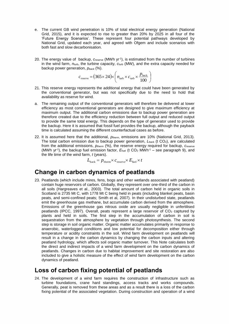
e. The current GB wind penetration is 10% of total electrical energy generation (National Grid, 2015), and it is expected to rise to greater than 20% by 2025 in all four of the ‘Future Energy Scenarios’. These represent four potential pathways developed by National Grid, updated each year, and agreed with Ofgem and include scenarios with both fast and slow decarbonisation.

20. The energy value of backup, creserve (MWh yr-1), is estimated from the number of turbines in the wind farm, nturb, the turbine capacity, cturb (MW), and the extra capacity needed for backup power generation, pback (%).

10024365 back

turbturbreserve

pcnc

21. This reserve energy represents the additional energy that could have been generated by the conventional generator, but was not specifically due to the need to hold that availability as reserve for wind.

a. The remaining output of the conventional generators will therefore be delivered at lower efficiency as most conventional generators are designed to give maximum efficiency at maximum output. The additional carbon emissions due to backup power generation are therefore created due to the efficiency reduction between full output and reduced output to provide the same total energy. This depends on the type of generator used to provide the backup. Here it is assumed that fossil fuel provides the backup, although the payback time is calculated assuming the different counterfactual cases as before.

22. It is assumed here that the additional, ptherm, emissions are 10% (National Grid, 2013). The total carbon emission due to backup power generation, Lback (t CO2), are calculated from the additional emissions, ptherm (%), the reserve energy required for backup, creserve (MWh yr-1), the backup fuel emission factor, Efuel (t CO2 MWh-1 – see paragraph 9), and the life time of the wind farm, t (years).

tEcpL fuelreservethermback

Change in carbon dynamics of peatlands

23. Peatlands (which include mires, fens, bogs and other wetlands associated with peatland) contain huge reservoirs of carbon. Globally, they represent over one-third of the carbon in all soils (Hargreaves et al., 2003). The total amount of carbon held in organic soils in Scotland is 2735 Mt C, with 1778 Mt C being held in peats (including blanket peats, basin peats, and semi-confined peats; Smith et al, 2007). In their undisturbed state, peatlands emit the greenhouse gas methane, but accumulate carbon derived from the atmosphere. Emissions of the greenhouse gas nitrous oxide are usually negligible in unfertilised peatlands (IPCC, 1997). Overall, peats represent a large reservoir of CO2 captured by plants and held in soils. The first step in the accumulation of carbon in soil is sequestration from the atmosphere by vegetation through photosynthesis. The second step is storage in soil organic matter. Organic matter accumulates primarily in response to anaerobic, waterlogged conditions and low potential for decomposition either through temperature or acidity constraints in the soil. Wind farm development on peatlands will result in a change in the carbon dynamics by changing the carbon inputs and altering peatland hydrology, which affects soil organic matter turnover. This Note calculates both the direct and indirect impacts of a wind farm development on the carbon dynamics of peatlands. Changes in carbon due to habitat improvement and site restoration are also included to give a holistic measure of the effect of wind farm development on the carbon dynamics of peatland.

Loss of carbon fixing potential of peatlands

24. The development of a wind farm requires the construction of infrastructure such as turbine foundations, crane hard standings, access tracks and works compounds. Generally, peat is removed from these areas and as a result there is a loss of the carbon fixing potential of the associated vegetation. During construction and operation of a wind

farm, the soil may be drained by design or unintentionally. Drainage has significant effects on the vegetation of peatlands (Stewart and Lance, 1991). Here, the loss of the carbon fixing potential of the peatland is calculated for the area from which peat is removed and also for the area affected due to drainage.

25. The estimated global average for the apparent carbon accumulation rate in peatland ranges from 0.12 to 0.31 t C ha-1 yr-1 (Turunen et al., 2001; Botch et al., 1995). If it is available, site specific data can be used. However, this loss represents a very small proportion of the total emissions, so the mid-range value used in the previous guidance (0.25 t C ha-1 yr-1 = 0.92 t CO2 ha-1 yr-1) provides an adequate estimate. Loss of carbon fixing potential of peatland, Lfix (t CO2), is calculated from the area affected by wind farm development (both directly by removal of peat, Adirect (ha – see paragraph 32), and indirectly by drainage Aindirect (ha – see paragraph 40)), the annual gains due to the carbon fixing potential of the peatland, Gbog (Gbog = 0.92 t CO2 ha-1 yr-1), and the time required for habitat restoration, trestore (years).

restorebogindirectdirectfix tGAAL

Changes in carbon stored in peatlands Note: this carbon represents the greatest risk in terms of potential loss of carbon dioxide because peat takes a long time to accumulate in temperate regions and hence site restoration and carbon savings need to reflect this.

26. During wind farm construction, carbon is lost directly from the excavated peat and indirectly from the area affected by drainage.

27. The potential impact of peat removal is estimated from the volume of peat removed by different practices. Loss of carbon from the excavated peat is assumed to be 100%. If the excavated carbon is later restored, so potentially reducing the carbon losses from excavated peat, this is added to the area and depth of the improved site. This allows good peat preservation practices to be accounted for in the C emission savings.

28. Indirect loss of carbon due to drainage is estimated using default values from the Intergovernmental Panel on Climate Change (IPCC) (IPCC, 1997) as well as by more site specific equations derived from the scientific literature (Smith et al., 2007; Nayak et al., 2008).

29. Carbon gains due to habitat improvement are similarly estimated using IPCC default values (IPCC, 1997) and the more site specific equations derived from the scientific literature (Smith et al., 2007; Nayak et al., 2008).

Loss of carbon from removed peat

30. The total volume of peat removed during construction, Vdirect (m3), is calculated from the dimensions of structures introduced to the site during development (average length, li (m), width, wi (m), and depth, dpeat,i (m) of each construction, i). Borrow pits, turbine foundations, hard-standing area and access tracks are currently included in the spreadsheet.

i

ipeat,iidirect dwlV

The total area of peat removed, Adirect (m2), is calculated similarly using average length and width.

If the length and width at the bottom is less than at the surface, this is accounted for in the calculation of volume.

The volume and area of any additional peat excavated can also be entered directly.

31. Loss of carbon from the removed peat, Ldirect (t CO2), is assumed to be 100%. If peat is later returned to the site with full restoration of the habitat and hydrological conditions, the volume of restored peat is added to the calculation of C emission savings due to site

improvement. However, for this option to be used, the restoration plan should demonstrate a high probability that peat hydrology will be restored and disturbance of peat minimised.

32. Loss of carbon from the removed peat, Lremoved (t CO2), is calculated from the carbon content of dry peat, pCdrypeat (%), the dry soil bulk density (dried to a constant weight at

105C), BDdrysoil (g cm-3), and the volume of peat removed, Vdirect (m3).

directsoildry peatdry removed100

667.3VBDpCL

When flooded, peat soils emit less carbon dioxide but more methane than when drained. In flooded soils, carbon dioxide emissions are usually exceeded by plant fixation, so the net exchange of carbon dioxide with the atmosphere is negative and soil carbon stocks increase. When soils are aerated carbon dioxide emissions usually exceed plant fixation, so the net exchange of carbon dioxide with the atmosphere is positive. To calculate the carbon emissions attributable to removal of the peat only, Ldirect (t CO2 eq.), any emissions occurring if the soil had remained in situ and undrained are subtracted from the emissions occurring after removal.

undrainedremoveddirect LLL

Calculation of the losses from undrained soil is described in paragraph 45.

Loss of carbon from drained peat

Estimation of volume of peat affected by drainage

33. The extent of drainage around the site of construction strongly influences the total volume of peat impacted by the construction of the wind farm. Where sufficient measurements are available to describe the hydrological features of the wind farm area, this should be used together with a detailed hydrological model to simulate the likely changes in peat hydrology. If insufficient measurements are available, a worst case estimate of extent of drainage around the development features should be used.

34. The volume of peat affected by drainage is calculated assuming the additional drained zone of edrain (m) on each side of the construction. The depth of drainage is assumed to show a linear decline from the edge and depth of the drainage feature to the water table depth at the extent of drainage. Note that the area where peat is removed should not be included because carbon loss from removed peat has already been counted in direct losses. The calculation of volume affected by drainage, Vindirect,i (m3), uses the extent of drainage, edrain (m), average length, li (m), width, wi (m), and depth of drainage, ddrain,i (m) for each construction feature, i.

35. For borrow pits, and turbine and hard-standing foundations, the depth of drainage, ddrain,i (m), is assumed to be equivalent to the depth of the construction. The calculation uses the following equation.

iiidrainidraindrain,iindirect, 225.0 wlweledV i

(equation for turbine and hard-standing foundations)

The volume drained around switching stations, site compounds and lay-down areas can be calculated similarly. If permanent drainage around foundations and hard-standing is not required, the area should be assumed to be drained only up to the time of completion of backfilling, removal of any temporary surface drains, and full restoration of the hydrology. The carbon losses are then reduced from the restored area as discussed in paragraphs 42 to 56.

36. For access tracks, the depth of any drainage and the area included is dependent on the type of track. For excavated and rock-filled roads, the depth of drainage, ddrain,i (m), is assumed to be equivalent to the depth of the track. The peat removed or displaced by construction of the track is not included in the drained volume. The volume affected by drainage is calculated using the following equation.

drainiidrain,iindirect, 25.0 eldV

(equation for cable trenches, excavated and rock-filled roads)

The volume affected by drainage around cable trenches with permeable linings (e.g. sand) that deviate from the lines of tracks should also be calculated using the above equation.

37. For floating roads, drainage is only included for the length of track that has been specifically drained, and the depth of drains is taken to be as specified for the drains. Since floating roads are known to sink in many cases, evidence should be provided about the risk of requirements for additional drainage. The volume affected by drainage is calculated using the following equation.

idrainiidrain,iindirect, 25.0 weldV

(equation for floating roads)

38. The total volume of peat affected by drainage, Vindirect (m3), is the sum of the volumes of peat affected around each type of construction, Vi,indirect (m3).

i

VV iindirect,indirect

The total area of peat affected by drainage, Aindirect (m2), is calculated similarly from the length and width of constructions and the estimated extent of drainage.

Loss of carbon from drained peat if the site is not restored after decommissioning

39. When flooded soils are drained, loss of soil carbon continues until a new stable state is reached. For peats, this is close to 0% carbon (IPCC, 1997). Therefore, if the site is not restored after decommissioning of the wind farm, it is assumed that 100% of the carbon will be lost from the drained volume of soil. The loss of carbon from the drained peat, Ldrained (t CO2), is calculated from the carbon content of dry peat, pCdry peat (%), the dry soil

bulk density (dried to a constant weight at 105C), BDdry soil (g cm-3), and the volume of peat drained, Vindirect (m3).

indirectsoildry peatdry drained100

667.3VBDpCL

Loss of carbon from drained peat if the site is restored after decommissioning

40. Restoration of the site could potentially halt carbon loss processes, allowing carbon dioxide emissions to be limited to the time before the habitat and hydrological conditions are restored. The amount of carbon lost is then calculated from the annual emissions of methane, ECH4 (t CO2 eq. ha-1 yr-1), and carbon dioxide, ECO2 (t CO2 ha-1 yr-1), the area of drained peat, Aindirect (ha), and the time until the site is restored, t (years). However, for this option to be used, the restoration plan should demonstrate a high probability that peat hydrology will be restored across the site (water table at the surface for over 50% of the year), disturbance of the remaining peat will be minimised, and peat forming vegetation will develop in areas from which peat was removed or drained. If restoration of the site is inadequate, the amount of carbon lost will be in between the range of values calculated for restored (paragraph 46) and non-restored sites (paragraph 41).

41. Methane emissions are calculated using the following equation:

CO2CCH4F

CH4CH4365

CD

RE

where ECH4 is the total annual emissions of CH4 (t CO2 eq. ha-1 yr-1), RCH4 is the annual rate of CH4 emissions (t CH4-C ha-1 yr-1), DF is the number of days in the year that the

land is flooded, and CCH4-CCO2 converts CH4-C to CO2 equivalents (CCH4-CCO2 = 30.67

CO2 eq. (CH4-C)-1). The emission factors used (RCH4, and DF) differ between drained and undrained conditions as described in paragraphs 49 to 54.

42. Carbon dioxide emissions are calculated using the following equation:

365

365 FCO2CO2

DRE

where ECO2 is the total annual emissions of CO2 (t CO2 ha-1 yr-1), RCO2 is the annual rate of carbon dioxide emission (t CO2 ha-1 yr-1), DF is the number of days in the year that the land is flooded. The emission factors used (RCO2, and DF) differ between drained and undrained conditions as described in paragraphs 49 to 54.

43. The total loss of carbon from the peat before drainage, Lundrained (t CO2 eq.), is calculated from the annual emissions of methane, ECH4 (t CO2 eq. ha-1 yr-1), the annual emissions of carbon dioxide, ECO2 (t CO2 ha-1 yr-1), the area to be drained, Aindirect (ha), and the time to restoration (assumed to be the life time of the wind farm), t (years).

tAEEL indirectCO2CH4undrained

44. The total loss of carbon from the drained peat, Ldrained (t CO2 eq.), is calculated, using the same equation, but calculating the annual emissions of carbon dioxide, ECO2 (t CO2 ha-1 yr-1) and methane, ECH4 (t CO2 eq. ha-1 yr-1) for a drained soil. Methane emissions will be negative or close to zero due to oxidation of methane by the soil.

tAEEL indirectCO2CH4drained

45. Peat soils emit less carbon dioxide but more methane when flooded than drained. In flooded soils, carbon dioxide emissions are usually exceeded by plant fixation, so the net exchange of carbon dioxide with the atmosphere is negative and soil carbon stocks increase. In drained soils, carbon dioxide emissions usually exceed plant fixation, so the net exchange of carbon dioxide with the atmosphere is positive. To calculate the carbon emissions attributable to drainage only, Lindirect (t CO2 eq.), any emissions occurring if the soil had remained undrained are subtracted from the emissions occurring after drainage.

undraineddrainedindirect LLL

46. The annual emissions of methane and carbon dioxide can be estimated either using the IPCC default methodology (IPCC, 1997), or using more site specific equations derived from the scientific literature (Nayak et al., 2008).

Calculation of changes in methane and carbon dioxide emissions from drained peat based on IPCC Guidelines

47. The IPCC default factors for acid bogs and fens in cool temperate zones used in paragraphs 43 and 44 are given in Table 3. When the soil is undrained, the period of flooding is based on the monthly mean temperature and the length of inundation. When the soil is drained, the period of flooding is assumed to be zero (DF = 0 days yr-1).

Acid Bogs Fens

Number of days in the year that land is flooded, DF 178 169

Annual rate of CO2 emissions from drained soils, RCO2 (t CO2 ha-1 yr-1) 35.2 35.2

Annual rate of CH4 emissions from flooded soils, RCH4 (t CH4-C ha-1 yr-1)

4.015 x 10-2 0.219

Table 3. IPCC default emission factors used to calculate methane and carbon dioxide emissions

48. These are widely accepted, generic emission factors, but the figures are averaged across cool temperate peatlands and allow no use of site specific information, such as water table depth before wind farm development. Under the impacts of climate change, or if the site is not a pristine peatland, the water table depth may already have been lowered before any drainage associated with the development. In this case, it is recommended that the more site specific factors given below are used as described in the next section.

Calculation of changes in methane and carbon dioxide emissions from drained peat using site specific equations

49. Methane emissions are calculated using the site specific equation described by Nayak et al. (2010). For acid bogs, the annual rate of methane emissions, RCH4, (t CH4-C (ha)-1 yr-1) is calculated as shown below.

67.36529.31001234.0exp1000

1waterCH4 TdR

where T is the average annual air temperature (C), pH is the soil pH and dwater is the water table depth (m). This equation was derived from 57 experimental measurements. The equation shows significant correlation with measurements (r2 = 0.54, P>0.05. By statistical convention, if P>0.05 this relationship can be considered to be highly significant. Evaluation against 29 independent experiments shows a significant association (r2=0.81; P>0.05) and an average error of 27 t CH4-C ha-1 yr-1

which is non-significant (P<0.05) (Smith et al., 1997).

50. For fens, the annual rate of methane emissions, RCH4, (t CH4-C (ha)-1 yr-1) is calculated as shown below.

TdR 662.0100097.0exp62.563101000

1waterCH4

where T is the average annual air temperature (C), pH is the soil pH and dwater is the water table depth (m). This equation was derived from 35 experimental measurements. The equation shows significant correlation with measurements (r2 = 0.41, P>0.05. Evaluation against 7 independent experiments shows a significant association (r2=0.69; P>0.05) and an average error of 164 t CO2 ha-1 yr-1

(significance not defined due to lack of replicates) (Smith et al., 1997).

51. For acid bogs, the annual rate of carbon dioxide emissions, RCO2, (t CH4-C (ha)-1 yr-1) is calculated as shown below.

80054.72501000515.0exp26.0exp67001000

667.3waterCO2 TdR

where T is the average annual air temperature (C), pH is the soil pH and dwater is the water table depth (m). This equation was derived from 60 experimental measurements. The equation shows significant correlation with measurements (r2 = 0.53, P>0.05. Evaluation against 29 independent experiments shows a significant association (r2=0.21; P>0.05) and an average error of 3023 t CO2 ha-1 yr-1

which is non-significant (P<0.05) (Smith et al., 1997).

52. For fens, the annual rate of carbon dioxide emissions, RCO2, (t CO2-C (ha)-1 yr-1) is calculated as shown below.

TdR 23.15350100073.0exp175.0exp16244.1000

667.3waterCO2

where T is the average annual air temperature (C), pH is the soil pH and dwater is the water table depth (m). This equation was derived from 44 experimental measurements. The equation shows significant correlation with measurements (r2 = 0.42, P>0.05. Evaluation against 18 independent experiments shows a significant association (r2=0.56; P>0.05) and an average error of 2108 t CO2 ha-1 yr-1

(significance not defined due to lack of replicates) (Smith et al., 1997).

53. The experimental data used to derive the above equations were collated during the development and evaluation of the ECOSSE model (Smith et al., 2007). Note that further improvement in a site specific estimate of methane, carbon dioxide and dissolved organic carbon losses could be obtained using measurements taken at the site to run a peer-reviewed and proven model of carbon dynamics, such as ECOSSE.

54. These more site specific annual emission rates are used in the equations given in paragraphs 43 and 44, assuming days of flooding, DF, given in Table 2 to estimate annual emissions of carbon dioxide and methane.

Loss of carbon dioxide due to leaching of dissolved and particulate organic carbon

55. Lowering the water table by drainage may reduce the potential for dissolved and particulate organic carbon retention within the soil (e.g. Holden et al., 2004; Worrall et al., 2004) as well as increasing the decomposition rates (due to increased aeration). A recent study by Wallage et al. (2006) confirms that losses of dissolved organic carbon are higher from drained than undrained peats. Losses of carbon dioxide due to leaching of dissolved organic carbon, LDOC (t CO2), are calculated by multiplying the sum of the gaseous losses of carbon from the different sources in the soil, Lgas (t C), by the percentage of the total gaseous loss of carbon that is leached as dissolved organic carbon, pDOC (%), and the percentage of leached dissolved organic carbon that is emitted as carbon dioxide,

pDOCCO2 (%).

gas

DOCCO2DOC

DOC100

667.3 Lpp

L

56. Losses due to leaching of dissolved organic carbon are assumed to be less than 26% of total gaseous carbon loss from the drained, restored and improved habitat peat land (pDOC = 10) following the work of Worrall et al. (2009). It is assumed that 100% of the

dissolved organic carbon is emitted as carbon dioxide (pDOCCO2 = 100). Losses of particulate organic matter are calculated similarly, assuming the percentage loss is less than 8% of the total gaseous carbon losses after Worrall et al. (2009).

57. In the example, total gaseous emissions of carbon were small, resulting in low losses of dissolved organic carbon. This was due to the large proportion of the site that was improved.

Loss of carbon due to peatslide

58. The Scottish Executive (2006) has established a rigorous procedure for identifying existing, potential and construction induced peat landslide hazards. This should lead to a reduced likelihood of peat landslides occurring due to the wind farm development. Any drainage measures used to mitigate the risk should be accounted for using the methods described in paragraphs 42 to 56. It is assumed that the required measures to avoid peat landslides have been taken, so that the risk of peat landslide is minimal. Therefore this potential source of carbon loss is omitted from the guidance. Note that less catastrophic erosion losses, such as those due to collapse of gullies, is not covered by the procedures to reduce peat landslides, but has not yet been included in this guidance.

Changes of carbon due to forestry clearance

59. The presence of extensive areas of forestry on and in the vicinity of the wind farm site can significantly reduce the yield of wind energy, so it may be necessary to clear existing forestry. The losses of carbon from tree biomass depend on the fate of wood products following felling. Forestry may be felled earlier than planned due to the wind farm development, so limiting the nature and longevity of wood products. If a forestry plantation was due to be felled with no plan to replant, the effect of the land use change is not attributable to the wind farm development and should be omitted from the calculation. If, however, the forestry is felled for the development, changes in timber, residues and changes in soil conditions are attributable to the wind farm and should be accounted for.

60. The amount of carbon loss from timber and residues depends on the type of tree, the age of crop on felling, the end use of the timber and how quickly any stored carbon is returned to the atmosphere (Cannell, 1999). Losses from forestry are calculated from either a

simple forest C loss calculation (Sheet 7i) or a more detailed forest C loss calculation (Sheet 7ii). The advantages of the detailed method of forest carbon accounting can be summarised as (1) an enhanced calculation of forest growth forgone, including broad-scale capture of influence of site, and calibration for two conifer species, (2) the ability to grow short rotation forestry after forest clear-felling, (3) the potential to account for felled woody biomass, as a net gain to the developer, through provision as woody biomass for biofuel (a consistent approach with an immediate short-term carbon benefit) and (4) an incorporation of forest management (tree height impact) on turbine output via a simple wind speed ratio approach.

61. Loss of carbon dioxide due to forestry clearance, Lforest (t CO2) is calculated in both methods from the area of forestry to be felled, Aforest (ha), the average carbon sequestered per year, Gforest (t CO2 ha-1 yr-1) and the lifetime of the wind farm, t (years).

tGAL forestforestforest

The methods differ in the approach used to calculate Gforest.

Simple method for calculating carbon sequestered in forestry

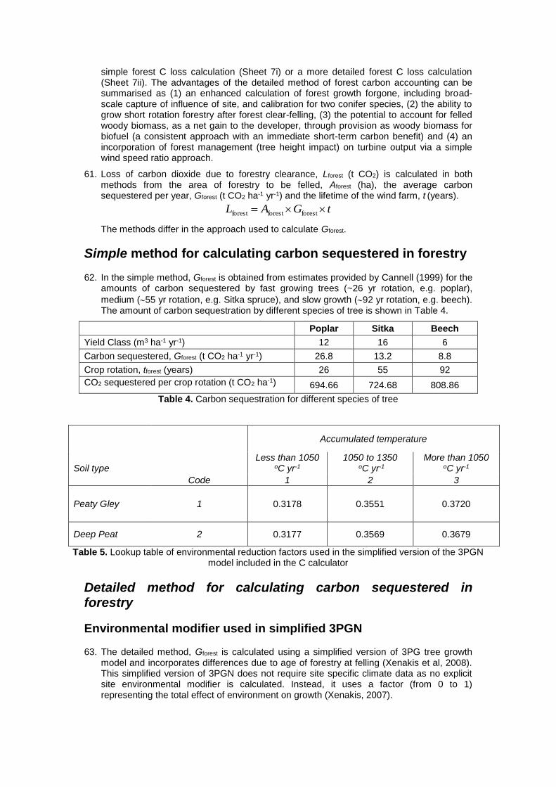
62. In the simple method, Gforest is obtained from estimates provided by Cannell (1999) for the amounts of carbon sequestered by fast growing trees (~26 yr rotation, e.g. poplar),

medium (55 yr rotation, e.g. Sitka spruce), and slow growth (92 yr rotation, e.g. beech). The amount of carbon sequestration by different species of tree is shown in Table 4.

Poplar Sitka Beech

Yield Class (m3 ha-1 yr-1) 12 16 6

Carbon sequestered, Gforest (t CO2 ha-1 yr-1) 26.8 13.2 8.8

Crop rotation, tforest (years) 26 55 92

CO2 sequestered per crop rotation (t CO2 ha-1) 694.66 724.68 808.86

Table 4. Carbon sequestration for different species of tree

Detailed method for calculating carbon sequestered in forestry

Environmental modifier used in simplified 3PGN

63. The detailed method, Gforest is calculated using a simplified version of 3PG tree growth model and incorporates differences due to age of forestry at felling (Xenakis et al, 2008). This simplified version of 3PGN does not require site specific climate data as no explicit site environmental modifier is calculated. Instead, it uses a factor (from 0 to 1) representing the total effect of environment on growth (Xenakis, 2007).

Accumulated temperature

Soil type Less than 1050

oC yr-1 1050 to 1350

oC yr-1 More than 1050

oC yr-1

Code 1 2 3

Peaty Gley 1 0.3178 0.3551 0.3720

Deep Peat 2 0.3177 0.3569 0.3679

Table 5. Lookup table of environmental reduction factors used in the simplified version of the 3PGN model included in the C calculator

Light Interception

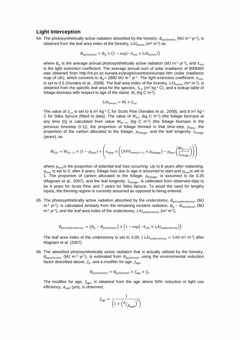
64. The photosynthetically active radiation absorbed by the forestry, ∅pa(forest) (MJ m-2 yr-1), is

obtained from the leaf area index of the forestry, 𝐿𝐴𝐼forest (m2 m-2) as

∅pa(forest) = ∅p × (1 − exp(−𝑘ext × 𝐿𝐴𝐼forest))

where ∅p is the average annual photosynthetically active radiation (MJ m-2 yr-1), and 𝑘ext

is the light extinction coefficient. The average annual sum of solar irradiance of 800kWh was obtained from http://re.jrc.ec.europa.eu/pvgis/countries/europe.htm (solar irradiance map of UK), which converts to ∅p= 2880 MJ m-2 yr-1. The light extinction coefficient, 𝑘ext,

is set to 0.5 (Xenakis et al., 2008). The leaf area index of the forestry, 𝐿𝐴𝐼forest (m2 m-2), is

obtained from the specific leaf area for the species, 𝑆𝐿𝐴 (m2 kg-1 C), and a lookup table of

foliage biomass with respect to age of the stand, 𝑊f (kg C m-2),

𝐿𝐴𝐼forest = 𝑊f × 𝑆𝐿𝐴.

The value of 𝑆𝐿𝐴 is set to 6 m2 kg-1 C for Scots Pine (Xenakis et al., 2008), and 8 m2 kg-1

C for Sitka Spruce (fitted to data). The value of 𝑊f(t) (kg C m-2) (the foliage biomass at

any time (t)) is calculated from value 𝑊f(t−1) (kg C m-2) (the foliage biomass in the

previous timestep (t-1)), the proportion of foliage thinned in that time-step, 𝑝thin, the

proportion of the carbon allocated to the foliage, 𝑝foliage, and the leaf longevity, 𝑙foliage

(years), as

𝑊f(t) = 𝑊f(t−1) × (1 − 𝑝thin) + (𝑛step × ((𝑁𝑃𝑃trees(t−1) × 𝑝foliage) − 𝑝loss (𝑊f(t−1)

𝑙foliage

)))

where 𝑝lossis the proportion of potential leaf loss occurring. Up to 6 years after replanting, 𝑝loss is set to 0, after 6 years, foliage loss due to age is assumed to start and 𝑝lossis set to

1. The proportion of carbon allocated to the foliage, 𝑝foliage, is assumed to be 0.25

(Magnani et al., 2007), and the leaf longevity, 𝑙foliage, is calibrated from observed data to

be 4 years for Scots Pine and 7 years for Sitka Spruce. To avoid the need for lengthy inputs, the thinning regime is currently assumed as opposed to being entered.

65. The photosynthetically active radiation absorbed by the understorey, ∅pa(understorey) (MJ

m-2 yr-1), is calculated similarly from the remaining incident radiation, ∅p − ∅pa(forest) (MJ

m-2 yr-1), and the leaf area index of the understorey, 𝐿𝐴𝐼understorey (m2 m-2),

∅pa(understorey) = (∅p − ∅pa(forest)) × (1 − exp(−𝑘ext × 𝐿𝐴𝐼understorey))

The leaf area index of the understorey is set to 3.00, ( 𝐿𝐴𝐼understorey = 3.00 m2 m-2) after

Magnani et al. (2007).

66. The absorbed photosynthetically active radiation that is actually utilised by the forestry, ∅pau(forest) (MJ m-2 yr-1), is estimated from ∅pa(forest) using the environmental reduction

factor described above, 𝑓𝐸, and a modifier for age, 𝑓age,

∅pau(forest) = ∅pa(forest) × 𝑓age × 𝑓𝐸.

The modifier for age, 𝑓age, is obtained from the age where 50% reduction in light use

efficiency, 𝐴half (yrs), is observed,

𝑓age = 1

(1 + (𝐴𝐴half

⁄ )4

)

where 𝐴 is the age of the stand (yrs). The value of 𝐴half is set to 100 years for Scots Pine (Xenakis et al., 2008), and 120 years for Sitka Spruce (Magnani et al., 2007)

67. The absorbed photosynthetically active radiation that is actually utilised by the understorey, ∅pau(understorey) (MJ m-2 yr-1), is estimated from ∅pa(understorey) using the

environmental reduction factor described above, 𝑓𝐸, but without a modifier for age as the understorey is assumed to regenerate each year,

∅pau(understorey) = ∅pa(understorey) × 𝑓𝐸.

Primary productivity 68. The gross primary production of trees, 𝐺𝑃𝑃trees (kg C m-2 yr-1), is calculated from

∅pau(forest) (MJ m-2 yr-1) using the maximum light use efficiency for the tree species, 𝜀 (kg

C MJ-1 day-1),

𝐺𝑃𝑃trees = 𝜀 × ∅pau(forest).

The value of 𝜀 -is assumed to be 0.00152 kg C MJ-1 day-1 for Scots Pine (Xenakis et al., 2008) and 0.00166 kg C MJ-1 day-1 for Sitka Spruce (Minnuno et al., 2010). The net primary production of the trees, 𝑁𝑃𝑃trees (kg C m-2 yr-1), can then be calculated

using a standard ratio for NPP:GPP, 𝑌 = 0.47 after Waring (2000) and Minnuno et al. (2010).

𝑁𝑃𝑃trees = 𝑌 × 𝐺𝑃𝑃trees. The net primary production of the understorey, 𝑁𝑃𝑃understorey (kg C m-2 yr-1), is calculated

similarly,

𝑁𝑃𝑃understorey = 𝑌 × 𝜀 × ∅pau(understorey).

The maximum light use efficiency, 𝜀 (kg C MJ-1 day-1), is currently assumed to be equivalent to the value given for the selected forestry species. The total net primary production of the forestry and understorey, 𝑁𝑃𝑃total (t C ha-1 yr-1), is then calculated by adding the net primary production of trees and understorey and multiplying by 10 to convert kg C m-2 yr-1 to t C ha-1 yr-1,

𝑁𝑃𝑃total = 10 × (𝑁𝑃𝑃trees + 𝑁𝑃𝑃understorey).

Cleared Forest Floor Emissions 69. Loss from soils of non-forested land is given by the estimated rate of C loss for two peat

depths taken from Zerva et al (2005) for peaty gley (peat depth 5 to 50cm = 3.98 t C ha-1 yr-1 ), and Hargreaves et al (2003) for deep peat (peat depth>50cm = 5.00 t C ha-1 yr-1).

Emissions from harvesting operations 70. Operational losses due to harvesting are provided by the user. Morison et al (2011) gives

emission factors for the UK. If clearfelling is assumed to be performed by harvester and timber is assumed extracted with forwarder, the emissions, Eharv (g CO2 m-3) are 6657 g CO2 m-3. The total emissions due to harvesting operations, Lharv (t CO2) are then given by

𝐿harv =𝑉harv × 𝐴harv × 𝐸harv

106

where 𝑉harv is the volume harvested in each hectare (m3 ha-1) and 𝐴harv is the area harvested (ha).

Savings from use of felled forestry as biofuel

71. Carbon savings can be accounted for in the C calculator due to the timber felled being used as a biofuel. The weight of biomass from the felled forestry, Wfelled (t), is given by the area of felled plantation, Afelled (ha), the carbon content of the felled forestry, Cfelled (t C ha-

1) and the C:biomass ratio of the felled forestry, rC:Biomass, as shown below

𝑊felled = 𝐴felled ×𝐶felled

𝑟C:Biomass.

Carbon in the felled forestry, Cfelled (t C ha-1), is calculated from the simplified 3PGN model described above. Wood biomass can be converted to dry weight using wood density based values from Lavers (1983) with a subsequent assumption that C:dry matter ratio is 50% (Matthews 1993) giving the C:biomass ratio, rC:Biomass. For simplicity an integrated factor, the ‘wood density to biomass factor’ taken from Mason et al. (2009) can be used to supply the value of rC:Biomass.

72. The assumption is for co-firing or delivery to a biomass specific electricity generating

station. Therefore, the savings in CO2 emissions associated with using the felled forestry as a biofuel, 𝑆felled→biofuel (t CO2) is calculated from the weight of biomass from the felled

forestry, Wfelled (t), the energy value of the felled forestry as a biomass fuel, 𝜖felled (MWh t-1) and the emission factor, Efuel (t CO2 MWh-1), for the counterfactual case

𝑆felled→biofuel = 𝑊felled × 𝜖felled × 𝐸fuel.

The counterfactual case is currently assumed in the C calculator to be fossil fuel-mix.

73. Carbon losses associated with transportation of woody biomass are calculated using transportation distance, Dtransport (km), and CO2 emissions due to transportation, Etransport (t CO2 km-1), and the weight of biomass from the felled forestry, Wfelled (t)

𝐿transport = 𝐷transport × 𝐸transport × 𝑊felled

𝐿transport = 𝐷transport × 𝐸transport

Assuming 20% of journey distance occurs on forest roads, Etransport can be assumed to be 3.933 t CO2 km-1 t-1 (Morison et al. 2011).

74. Net carbon losses associated with using the felled forestry as a biofuel, 𝐿felled→biofuel (t CO2), are then given by the difference between the losses associated with transportation, Ltransport (t CO2), and the savings due to using the felled forestry as a biofuel, 𝑆felled→biofuel (t CO2),

𝐿felled→biofuel = 𝐿transport − 𝑆felled→biofuel.

Savings from use of replanted forestry as a biofuel 75. Replanted forestry productivity is captured using the same simplified 3PGN model output

as described above. Productivity is again constrained by soil type and temperature. A wood density to biomass factor is applied as outlined above, as are emissions due to transport. This then allows the weight on felling of biomass from the replanted forestry, Wreplanted (t), to be obtained from the area of replanted forestry, Areplanted (ha), the carbon content of the replanted forestry, Creplanted (t C ha-1) and the C:biomass ratio of the replanted forestry, rC:Biomass, as shown below:

𝑊replanted = 𝐴replanted ×𝐶replanted

𝑟C:Biomass

76. Similarly, the savings in CO2 emissions associated with using the replanted forestry as a biofuel, 𝑆replanted→biofuel (t CO2) is calculated from the weight of biomass from the

replanted forestry, Wreplanted (t), the energy value of the replanted forestry as a biomass fuel, 𝜖replanted (MWh t-1) and the emission factor, Efuel (t CO2 MWh-1), for the counterfactual

case. 𝑆replanted→biofuel = 𝑊replanted × 𝜖felled × 𝐸fuel

77. Net carbon losses associated with using the replanted forestry as a biofuel,

𝐿replanted→biofuel (t CO2), are then given by the difference between the losses associated

with transportation, Ltransport (t CO2) (calculated as outlined above), and the savings due to using the felled forestry as a biofuel, 𝑆replanted→biofuel (t CO2),

𝐿replanted→biofuel = 𝐿transport − 𝑆replanted→biofuel

Total carbon loss associated with forest management

78. The total carbon losses associated with forest management, 𝐿forest(t CO2) is then given by the sum of all the parts described above

𝐿forest = 𝐿harv + 𝐿floor + 𝐿felled→biofuel + 𝐿replanted→biofuel

where 𝐿harv (t CO2) are the losses due to harvesting operations, 𝐿floor (t CO2) are the

emissions from the cleared forest floor, 𝐿felled→biofuel (t CO2) are the losses associated with using felled forestry as a biofuel, and 𝐿replanted→biofuel (t CO2) are the losses

associated with using replanted forestry as a biofuel.

Impacts of forestry management on windfarm carbon emission savings

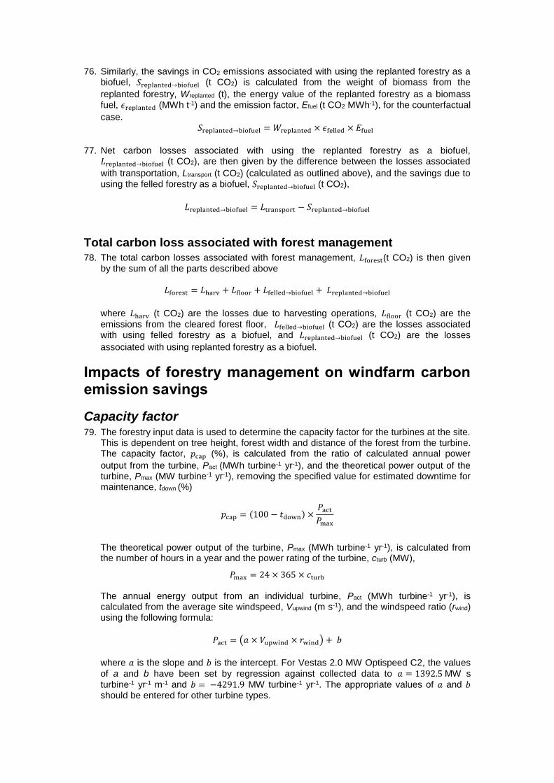
Capacity factor 79. The forestry input data is used to determine the capacity factor for the turbines at the site.

This is dependent on tree height, forest width and distance of the forest from the turbine. The capacity factor, 𝑝cap (%), is calculated from the ratio of calculated annual power

output from the turbine, Pact (MWh turbine-1 yr-1), and the theoretical power output of the turbine, Pmax (MW turbine-1 yr-1), removing the specified value for estimated downtime for maintenance, tdown (%)

𝑝cap = (100 − 𝑡down) ×𝑃act

𝑃max

The theoretical power output of the turbine, Pmax (MWh turbine-1 yr-1), is calculated from the number of hours in a year and the power rating of the turbine, cturb (MW),

𝑃max = 24 × 365 × 𝑐turb

The annual energy output from an individual turbine, Pact (MWh turbine-1 yr-1), is calculated from the average site windspeed, Vupwind (m s-1), and the windspeed ratio (rwind) using the following formula:

𝑃act = (𝑎 × 𝑉upwind × 𝑟wind) + 𝑏

where 𝑎 is the slope and 𝑏 is the intercept. For Vestas 2.0 MW Optispeed C2, the values

of a and b have been set by regression against collected data to 𝑎 = 1392.5 MW s

turbine-1 yr-1 m-1 and 𝑏 = −4291.9 MW turbine-1 yr-1. The appropriate values of 𝑎 and 𝑏 should be entered for other turbine types.

Windspeed ratio 80. The windspeed ratio (rwind) is the ratio of the windspeed downwind of the forestry,

𝑉downwind (m s-1), to the windspeed upwind of the forestry, Vupwind (m s-1),

𝑟 wind =𝑉downwind

𝑉upwind

Relative windspeed

81. Windspeed over a particular surface, 𝑉surface (m s-1), can be calculated for a particular hub-height, 𝐻hub (m), using the following simple relationship (Pal Ayra, 1988; Gardiner, 2004),

𝑉surface =𝑉Hnoeffect

× ln ((𝐻hub − ∆𝐻zero)

𝑅surface⁄ )

𝑘Von Karmen

where 𝑅surface is the aerodynamic roughness of the ground surface(m), 𝑘Von Karmen is the

Von Karman constant (𝑘Von Karmen = 0.4), ∆𝐻zero (m) is the zero plane displacement over

the particular surface, and 𝑉HIBL (m s-1) is the friction velocity (the windspeed at the height

𝐻IBL (m) of the internal boundary layer where there is no effect of the surface roughness).

Relative upwind windspeed 82. Because we are only interested in calculating the windspeed ratio, this can be simplified

by calculating the relative windspeed upwind and downwind of the forestry, 𝑉upwind(rel)

and 𝑉downwind(rel) respectively (m), by assuming 𝑉HIBL= 1 and ∆𝐻zero(surface) = 0.

𝑉upwind(rel) =ln (

𝐻hub𝑅upwind

⁄ )

𝑘Von Karmen

where 𝑅upwind is the aerodynamic roughness of ground upwind of the forestry (m),

assumed to be rough grass, giving an aerodynamic roughness of 0.03 m (Pal Ayra, 1988).

Relative downwind windspeed 83. If the hub-height, Hhub (m), is greater than the tree height at the end of the windfarm life,

Htree (m), the windspeed downwind of the forestry, replanted forest or felled forestry,

𝑉downwind(rel) (m), is calculated as

𝑉downwind(rel) = 𝑉HIBL× (

ln ((𝐻hub − ∆𝐻zero)

𝑅surface⁄ )

ln ((𝐻IBL − ∆𝐻zero)

𝑅surface⁄ )

)

where 𝑅surface (m) is the aerodynamic roughness of the surface, ∆𝐻zero (m) is the zero

plane displacement over the ground surface, and 𝑉HIBL is the windspeed at the height

where there is no effect of the roughness of the ground surface, 𝐻IBL (m) (i.e. the height

of the new internal boundary layer). For forestry, 𝑅surface is given by the aerodynamic

roughness of forestry, 𝑅forest (m), and is assumed to be 7.5% of the tree height, 𝐻tree (m), at the end of the windfarm life, 𝑅forest = 0.075 × 𝐻tree (m). Tree height is obtained from Forestry Commission growth and yield tables (Edwards and Christie, 1981), and averaged over the lifetime of the development. Similarly, for replanted forestry, 𝑅surfaceis given by the aerodynamic roughness of the replanted forestry, 𝑅replant = 0.075 × 𝐻tree

(m). For the felled area, 𝑅surfaceis given by the aerodynamic roughness of the felled area,

𝑅felled (m), which is assumed to be equivalent to the aerodynamic roughness of the ground upwind of the forestry, 𝑅felled = 𝑅upwind = 0.03 The zero plane displacement is

assumed to be 65% of the tree height,∆𝐻zero = 0.65 × 𝐻tree, unless tree height is less than 0.1 m, in which case it is assumed to be the aerodynamic roughness of ground upwind of the forestry, ∆𝐻zero = 𝑅upwind (m)). Note for replanted forestry and felled areas,

∆𝐻zero is approximated to zero in the above equation. 84. For forestry, if the hub-height, 𝐻hub (m), is less than the tree height at the end of the

windfarm life, 𝐻tree (m), then 𝑉downwind is given by

𝑉downwind(rel) = 𝑉HIBL× exp ((𝛼 ×

𝐻hub𝐻tree

⁄ ) − 1) × (ln (

(𝐻hub − ∆𝐻zero)𝑅forest

⁄ )

ln ((𝐻IBL − ∆𝐻zero)

𝑅forest⁄ )

)

where 𝛼 is an exponential decay factor for the wind profile over forest, currently assumed to be 4 (Pal Ayra, 1988; Cionco, 1965).

85. For replanted forestry and felled areas, there is no modification to the equation for 𝐻hub >𝐻tree. The height of the internal boundary layer, 𝐻IBL (m), is calculated as

𝐻IBL = ((0.75 + 0.03 × ln (𝑅upwind

𝑅surface

)) × 𝑅surface × (𝐷width

𝑅surface

)0.8

) + ∆𝐻zero

where 𝑅upwind (m) is the aerodynamic roughness of ground upwind of the forestry, 𝑅surface

is the aerodynamic roughness of the surface and 𝐷width (m) is the width of the area being

considered. If 𝐻IBL (m) is greater than the height of the maximum allowed top of the

internal boundary layer, 𝐻IBL(max) (assumed here to be 5000 m, Kaimal and Finnigan,

1994), then 𝐻IBL is set to HIBL(max). The value for the friction velocity (𝑉HIBL) is then

obtained from the upwind velocity (𝑉upwind) at height of the internal boundary layer, 𝐻IBL

(m). 86. In the case of forestry, 𝑅surface = 𝑅forest, and 𝐷width (m) is the width of forest around the

felled area i.e.

𝐻IBL(forest) = ((0.75 + 0.03 × ln (𝑅upwind

𝑅forest)) × 𝑅forest × (

𝐷width

𝑅forest)

0.8

) + ∆𝐻zero.

The height of the internal boundary layer over replanted forestry, 𝐻IBL(replant) (m), is

calculated similarly, using the height of replanted trees at the end of the windfarm life as Htree (m), the aerodynamic roughness of the unfelled forestry, 𝑅forest (m), as 𝑅upwind, and

the aerodynamic roughness of the replanted forestry, 𝑅replant (m), as 𝑅surface, i.e.

.

𝐻IBL(replant) = ((0.75 + 0.03 × ln (𝑅forest

𝑅replant)) × 𝑅replant × (

𝐷width

𝑅replant)

0.8

) + ∆𝐻zero.

87. Over the felled area, the height of the internal boundary layer, 𝐻IBL(felled) (m), is calculated

using the aerodynamic roughness of the unfelled forestry, 𝑅forest (m), as 𝑅upwind, the

aerodynamic roughness of the replanted felled area, 𝑅felled (m), as 𝑅surface, and ∆𝐻zero is

obtained from the aerodynamic roughness of the felled area (∆𝐻zero = 𝑅felled), i.e.

𝐻IBL(felled) = ((0.75 + 0.03 × ln (𝑅forest

𝑅felled)) × 𝑅felled × (

𝐷width

𝑅felled)

0.8

) + 𝑅felled.

Carbon dioxide saving due to improvement of peatland habitat

88. Habitat improvement at disturbed sites can significantly impact carbon emissions, potentially preventing further losses and increasing carbon stored in the improved habitat. Carbon gains due to habitat improvement are estimated using IPCC default values

(paragraph 49; IPCC, 1997) and site specific equations derived from the scientific literature (paragraphs 51 to 56). Emissions of nitrous oxide are assumed to be negligible in unfertilised peatlands (IPCC, 1997). However, for this option to be used, the improvement plan should demonstrate a high probability that peat hydrology will be restored and disturbance of peat minimised, resulting in rapid decolonisation of the natural vegetation.

89. To calculate the carbon emissions attributable to improvement only, Limprovement (t CO2 eq.), any emissions occurring if the soil had remained drained are subtracted from the emissions occurring after flooding (negative, indicates a net reduction in emissions).

drainedundrainedtimprovemen LLL

90. The reduction in total greenhouse gas emissions are given below for the example wind farm using the IPCC default methodology and the site specific equations. Using fossil-fuel-mix as the counterfactual, the reduction in payback time amounts to 1.01 years using the IPCC methodology, and 1.78 years using the site specific approach.

Calculation of payback time for the example case-study wind farm

91. The carbon payback time for a wind farm is calculated by comparing the net loss of carbon from the site due to wind farm development, Ltot (t CO2 eq.), with the carbon savings achieved by the wind farm while displacing electricity generated from coal fired capacity, grid mix or fossil fuel mix.

Ltot = Llife + Lback + Lfix + Ldirect + Lindirect + LDOC + Lforest + Limprovement

where Llife is the total loss of C emission savings due to production, transportation, erection, operation and dismantling of the wind farm (t CO2 – see paragraph 18), Lback is

the total loss of carbon emission savings due to backup power generation (t CO2 – see paragraph 23), Lfix is the loss of carbon fixing potential of peatland (t CO2 – see paragraph 27), Ldirect is the loss of carbon from the removed peat (t CO2 – see paragraph 34), Lindirect

is the loss of carbon due drainage (t CO2 eq. – see paragraph 47), LDOC is the loss of carbon dioxide due to leaching of dissolved organic carbon (t CO2 – see paragraph 57), Lforest is the loss of carbon dioxide due to forestry clearance (t CO2 – see paragraph 63), Limprovement is the loss (negative = gain) of carbon emissions due to habitat improvement (t CO2 eq., see paragraph 91).

92. The calculation of total carbon dioxide emission savings and payback time for the example wind farm are shown below. Note the very short payback time, due to good practice in the use of floating roads and the large area of habitat improvement.

References Ardente F., Beccali M., Cellura M., Lo Brano V. (2008) Energy performance and life cycle assessment of an Italian

wind farm. Renewable and Sustainable Energy Reviews, 12: 200–217.

Baggott S.L., Cardenas L., Garnett E., Jackson J., Mobbs D.C., Murrells T., Passant N., Thomson A., Watterson J.D. (2007) UK Greenhouse Gas Inventory, 1990 to 2005. Annual Report for submission under the Framework Convention on Climate Change. London, HSO. ISBN 0-9554823-1-3. www.naei.org.uk/reports.php. Report AEAT/ENV/R/2429 13/04/2007

BERR (2008) UK Renewable Energy Strategy. www.berr.gov.uk/energy/sources/renewables/ strategy/page43356.html

Botch M.S., Kobak K.I., Vinson T.S., Kolchugina T.P. (1995) Carbon pools andaccumulation in peatlands of the Former Soviet Union. Global Biogeochemical Cycles, 9: 37-46.

Bradley, R.I., Milne, R. , Bell J., Lilly, A., Jordan, C. and Higgins, A. (2005). A soil carbon and land use database for the United Kingdom. Soil Use and Management, 21: 363–369.

Cannell, M.G.R. (1999) Growing trees to sequester carbon in the UK: answers to some common

Questions. Forestry, 72: 238-247.

Carbon Trust/Dti (2004), Renewables Network Impacts Study. http://www.carbontrust.co.uk/Publications/publicationdetail.htm?productid=CT-2004-03

Dale, L., Millborrow, D., Slark, R., Strbac, G. (2004) Total Cost Estimates for Large-Scale Wind Scenarios in UK, Energy Policy, 32: 1949-56.

Defra (2001) Climate Change Agreements: Guidance on converting electricity from dedicated supplies to primary energy. CCA 09, December 2001

Department for Business Enterprise & Regulatory Reform (2007). Digest of United Kingdom Energy Statistics http://stats.berr.gov.uk/energystats/dukes07.pdf

Department of Trade and Industry (DTI) (2006) Energy Trends, March 2006.

Department of Environment, Food and Rural Affairs (Defra) (2007). Guidelines to Defra’s GHG conversion factors for company reporting (Defra, June 2007)

Digest of the United Kingdom Energy Statistics (2007). Department for Business, Enterprise and Regulatory Reform. A National Statistics Publication, London, HSO. ISBN 9780115155208. http://www.berr.gov.uk/energy/statistics/source/electricity/page18527.html

Digest of the United Kingdom Energy Statistics (2013). Department for Business, Enterprise and Regulatory Reform. A National Statistics Publication, London, HSO. https://www.gov.uk/government/uploads/system/uploads/attachment_data/file/279523/DUKES_2013_published_version.pdf

Digest of the United Kingdom Energy Statistics (2014). Department for Business, Enterprise and Regulatory Reform. A National Statistics Publication, London, HSO. https://www.gov.uk/government/uploads/system/uploads/attachment_data/file/338750/DUKES_2014_printed.pdf

Digest of the United Kingdom Energy Statistics (2015). Department for Business, Enterprise and Regulatory Reform. A National Statistics Publication, London, HSO. https://www.gov.uk/government/uploads/system/uploads/attachment_data/file/450302/DUKES_2015.pdf

Dillon P.J., Molot L.A. (1997) Effect of landscape form on export of dissolved organic carbon, iron, and phosphorus from forested stream catchments. Water Resources Research, 33: 2591–2600.

Hargreaves K.J., Milne R., Cannell M.G.R. (2003) Carbon balance of afforested peatland in Scotland. Forestry ,76: 299-317.

Holden J., Chapman P.J., Labadz J.C. (2004) Artificial drainage of peatlands: hydrological and hydrochemical process and wetland restoration. Progress in Physical Geography, 28: 95-123.

International Panel on Climate Change, IPCC (1997) Revised 1996 IPCC guidelines for national greenhouse gas inventories workbook, vol. 2. Cambridge, UK. Cambridge University Press.

IUCN UK Committee Peatland Programme Briefing Note No 1

http://www.iucn-uk-peatlandprogramme.org/sites/www.iucn-uk-peatlandprogramme.org/files/1%20Definitions%20final%20-%205th%20November%202014.pdf

Key Scottish Environment Statistics (2007) http://www.scotland.gov.uk/Publications/2007/08/20165714/0

Lenzen M., Munksgaard J. (2002) Energy and CO2 life-cycle analysesof wind turbines Review and applications. Renewable Energy, 26: 339-362.

Magnani F., Mencuccini M., Borghetti M., Berbigier P., Berninger F., Delzon S., Grelle A., Hari P., Jarvis P.G., Kolari P., Kowalski A.S., Lankreijer H., Law B.E., Lindroth A., Loustau D., Manca G., Moncrieff J.B., Rayment M., Tedeschi V., Valentini R., Grace J. (2007) The human footprint in the carbon cycle of temperate and boreal forests. Nature, 447: 848–850.

Minnuno F., Xenakis G., Perks M.P., Mencuccini M. (2010) Calibration and validation of a simplified process-based model for the prediction of the carbon balance of Scottish Sitka spruce (Picea sitchensis) plantations. Canadian Journal of Forest Research, 40: 2411-2426.

Morison J., Vanguelova E., Broadmeadow S., Perks M., Yamulki S., Randle T. (2010) Understanding the GHG implications of forestry on peat soils in Scotland. Forest Research Publication, pp. 55.

MLURI et al., (1991) xxx

National Grid (2013) , “Short Term Operating Reserve Carbon Intensity Report”http://www2.nationalgrid.com/WorkArea/DownloadAsset.aspx?id=40981

National Grid (2015) ‘Future Energy Scenarios, 2015’ http://fes.nationalgrid.com/

Nayak D.R., Miller D., Nolan A., Smith P., Smith J.U. (2008) Calculating Carbon Savings from Windfarms on Scottish Peatlands - Revision of Guidelines. October 2007 to January 2008. Final Report. RERAD UAB-016-07.

Nayak D.R., Miller D., Nolan A., Smith P., Smith (2010) Mires and Peat (Article 09), 4, 1-23, http://www.mires-and-peat.net/, ISSN 1819-754X

Renewable Energy Statistics Database for the UK (2008). http://www.restats.org.uk/obligations.htm

Scottish Executive (2006) http://www.scotland.gov.uk/Publications/2006/12/21162303/0

Scottish Government (2008) http://www.scotland.gov.uk/Topics/Business-Industry/Energy/Energy-sources/19185/17612

Scottish Government (2015) 2020 Routemap for Renewable Energy in Scotland – Update. http://www.gov.scot/Resource/0048/00485407.pdf

Scottish Natural Heritage (2007) Annual Review 2006/07. Scottish Natural Heritage, Battleby. pp 36.

Scottish Parliament (2011) http://www.parliament.scot/S4_EconomyEnergyandTourismCommittee/NATIONAL_GRID.pdf

Smith J.U., Smith P., Wattenbach M., Zaehle S., Hiederer R., Jones R.J.A., Montanarella L., Rounsevell M.D.A., Reginster I., Ewert F. (2005) Projected changes in mineral soil carbon of European croplands and grasslands, 1990-2080. Global Change Biology, 11: 2141–2152.

Smith J.U., Graves P., Nayak D.R., Smith P., Perks M., Gardiner B., Miller D., Nolan A., Morrice J., Xenakis S., Waldron S., Drew S. (2011) Carbon implications of windfarms located on peatlands – update of the Scottish Government Carbon Calculator tool. Final Report, RERAD Report CR/2010/05 (in press)

Smith P., Smith J.U., Wattenbach M., Meyer J., Lindner M., Zaehle S., Hiederer R., Jones R., Montanarella L., Rounsevell M., Reginster I., Kankaanpää S. (2006) Projected changes in mineral soil carbon of European forests, 1990-2100. Canadian Journal of Soil Science, 86: 159-169.

Smith P., Smith J.U., Flynn H., Killham K., Rangel-Castro I., Foereid B., Aitkenhead M., Chapman S., Towers W., Bell J., Lumsdon D., Milne R., Thomson A., Simmons I., Skiba U., Reynolds B., Evans C., Frogbrook Z., Bradley I., Whitmore A., Falloon P. (2007) ECOSSE: Estimating Carbon in Organic Soils - Sequestration and Emissions. Final Report. SEERAD Report. ISBN 978 0 7559 1498 2. 166pp.

Stewart A.J.A., Lance A.N. (1991) Effects of moor-draining on the hydrology and vegetation on northern Pennine blanket bog. Journal of Applied Ecology, 28: 1105-1117.

The Carbon Trust, (2007). http://www.carbontrust.co.uk/resource/measuring_co2/ Measuring_CO2_Examples.htm

The Concrete Centre , (2013) http://www.concretecentre.com/PDF/SCF_Table%207%20Embodied%20CO2_April%202013.pdf ).

Turunen J., Pitkänen A., Tahvanainen T., Tolonen K. (2001) Carbon accumulation in West Siberian mires, Russia. Global Biogeochemical Cycles, 15: 285-296.

Vestas (2005) Life Cycle Assessment of Offshore and Onshore Wind Power Plants Based on Vestas V90-3.0 MW Turbines. Vestas Wind Systems A/S, Randers, Denmark, 59 pp. Revision (2006): http://www.vestas.com/en/about-vestas/principles/sustainability/wind-turbines-and-the-environment/life-cycle-assessment-(lca).aspx

Wallage Z.E., Holden J., McDonald A.T. (2006) Drain blocking: An effective treatment for reducing dissolved organic carbon loss and water discolouration in a drained peatland. Science of the Total Environment, 367: 811-821.

Waring, R.H. (2000) A process model analysis of environmental limitations on the growth of Sitka spruce plantations in Great Britain. Forestry, 73: 65–79. doi:10.1093/forestry/73.1.65.

White S.W., Kulcinski, G.L. (2000) Birth to death analysis of the energy payback ratio and CO2 gas emission rates from coal, fission, wind, and DT fusion electrical power plants. Fusion Engineering Design, 48: 473-481.

White W.S. (2007) Net energy payback and CO2 emissions from three Midwestern wind farms: an update. Natural Resources Research, 15: 271 - 281.

Worrall F., Reed M., Warburton J., Burt T. (2003) Carbon budget for a British upland peat catchment. The Science of the Total Environment, 312: 133–146.

Worrall F., Harriman R., Evans C.D., Watts C., Adamson J., Neal C., Tipping E., Burt T.P., Grieve I., Montieth D., Naden P.S., Nisbet T., Reynolds B., Stevens P. (2004) Trends in dissolved organic carbon in UK rivers and lakes. Biogeochemistry, 70: 369-402.

Worrall F., Burt, T.P., Rowson, J.G., Warburton, J., Adamson,J.K. (2009) The multi-annual C budget of a peat covered catchment. Science of the Total Environment, 407: 4084–4094.

Xenakis G. (2007) Assessment of carbon sequestration and timber production of Scots pine across Scotland using the process-based model 3-PGN. Ph.D. Thesis. The University of Edinburgh, Edinburgh.

Xenakis G., Ray D., Mencuccini M. (2008) Sensitivity and uncertainty analysis from a coupled 3-PG and soil organic matter decomposition model. Ecological Modelling, 219: 1-16.