Embed Size (px)
Citation preview
Calculating the 3D magnetic field of ITER for European TBM studies
Simppa Akaslompoloa,∗, Otto Asuntaa, Thijs Bergmansa, Mario Gagliardib, Jose Galabertb, Eero Hirvijokia, Taina Kurki-Suonioa,Seppo Sipilaa, Antti Snickera, Konsta Sarkimakia
aDepartment of Applied Physics, Aalto University, FI-00076 AALTO, FINLANDbFusion for Energy, Barcelona, Spain
Abstract
The magnetic perturbation due to the ferromagnetic test blanket modules (TBMs) may deteriorate fast ion confinement in ITER.This effect must be quantified by numerical studies in 3D. We have implemented a combined finite element method (FEM) –Biot-Savart law integrator method (BSLIM) to calculate the ITER 3D magnetic field and vector potential in detail. Unavoidablegeometry simplifications changed the mass of the TBMs and ferritic inserts (FIs) up to 26%. This has been compensated for bymodifying the nonlinear ferromagnetic material properties accordingly. Despite the simplifications, the computation geometry andthe calculated fields are highly detailed. The combination of careful FEM mesh design and using BSLIM enables the use of thefields unsmoothed for particle orbit-following simulations. The magnetic field was found to agree with earlier calculations andrevealed finer details. The vector potential is intended to serve as input for plasma shielding calculations.
Keywords: ITER, Test Blanket Module, Magnetization, Ferritic Insert
1. Introduction
The goal of the fusion reactor ITER is to demonstrate the tech-nological and scientific feasibility of fusion energy. The fol-lowing reactor, DEMO, has a mission to demonstrate the large-scale production of electrical power and tritium fuel self-suf-ficiency. One of the tasks of ITER is to be a testbed for DEMOcomponents. ITER Test Blanket Modules (TBMs) will test thetechnology of tritium breeding modules for DEMO. Three ofthe eighteen ITER equatorial ports are reserved for these mod-ules. The material chosen for DEMO is ferritic steel [1]. There-fore, the ITER TBMs will be made of ferromagnetic materialthat will get magnetized by the tokamak magnetic fields. Theresulting local perturbation in the magnetic fields can deterio-rate the confinement of the plasma. Especially, the weakly col-lisional fast ions may find a local “hole” in the magnetic bottleand thus cause a hot spot on the first wall [2].
The TBM designs are checked for such threats by perform-ing simulations of fast ions [3, 4]. The key ingredient for thesimulations is a 3D magnetic field that includes the fields dueto the magnetized components. This paper describes a methodfor calculating the field due to ferromagnetic ITER components.The used geometry describes the ferritic inserts and test blanketmodules in detail. We also calculate another useful quantity:the magnetic vector potential – an important input for relatedplasma response calculations.
Input data. The key “raw” data we use to calculate the 3Dfield consists of the geometry and electric current in toroidal
∗Corresponding authorEmail address: [email protected] (Simppa
Akaslompolo)
field (TF) and poloidal field (PF) coils (including the centralsolenoid), the plasma equilibrium, and the geometry and mate-rial parameters of the ferromagnetic components. Two sets ofcomponents are considered: the TBMs and the ferritic inserts(FI) that are in place to reduce the variation of the toroidal fieldcaused by having only 18 discrete TF coils.
Methods. Our main tool is the commercial COMSOL Multi-physics finite element method (FEM) platform (ver. 4.4.0.195)and its AC/DC Module. For geometry simplifications we alsoused the SpaceClaim Engineer 3D direct modeler. In addition,MATLAB routines were used to prepare and deliver informa-tion to COMSOL as well as to build the COMSOL model.
No FEM calculation can match the precision of a directBiot-Savart law integration for magnetic fields from known coilgeometry. To capitalise on this, we utilise a two-step COM-SOL calculation: First we perform a magnetization calculation.Then a follow-up permanent magnet COMSOL calculation ex-tracts the field due to the magnetization from the results of themagnetization calculation. The permanent magnet results fromCOMSOL are finally superimposed on the Biot-Savart law in-tegrated fields. These fields are produced with the recently ex-tended BioSaw code [5].
In the magnetization calculation, the magnetic fields (mf)interface of the AC/DC module in COMSOL solves the vectorpotential A and the divergence control variable ψ from
∇ ×H(|B|) = Je + ∇ψ∇ × A = B
∇ · (A + ∇ψ) = 0. (1)
Symbol B denotes magnetic flux density and Je is the currentdensity in coils or plasma. The nonlinear magnetic proper-ties are described by the function H(|B|). At the boundaries
Preprint submitted to Fusion Engineering and Design, http: // dx. doi. org/ 10. 1016/ j. fusengdes. 2015. 05. 038 June 3, 2015
arX
iv:1
506.
0065
9v1
[ph
ysic
s.pl
asm
-ph]
1 J
un 2
015
of the computational domain, the boundary condition is set ton × A = 0, where n is the boundary’s normal vector. How-ever, the boundaries are effectively several kilometres from thetokamak, as will be explained in the context of equation 2.
The permanent magnet model can be considered a reducedversion of the above problem. We removed all coil and plasmacurrents and changed the constitutive relation inside the ferro-magnetic components to B = µ0 (H + M), where M is the mag-netization vector. COMSOL extracts the magnetization fromthe solution of the first step and effectively turns the ferromag-netic components into permanent magnets. The divergence con-dition variable is used for the permanent magnet model onlywhen the vector potential needs to be evaluated.
2. Geometry
In this section we describe each major component present in theFEM model. The description justifies and explains all simplifi-cations made to the geometry before importing it to COMSOL.
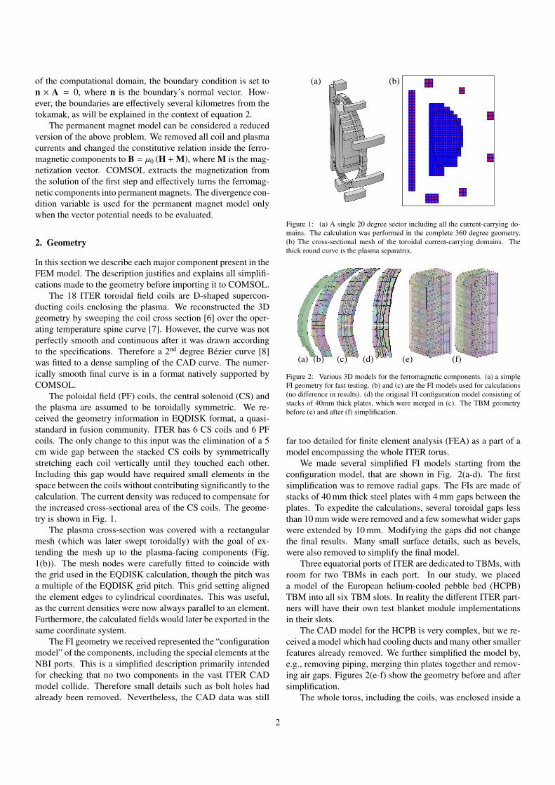
The 18 ITER toroidal field coils are D-shaped supercon-ducting coils enclosing the plasma. We reconstructed the 3Dgeometry by sweeping the coil cross section [6] over the oper-ating temperature spine curve [7]. However, the curve was notperfectly smooth and continuous after it was drawn accordingto the specifications. Therefore a 2nd degree Bezier curve [8]was fitted to a dense sampling of the CAD curve. The numer-ically smooth final curve is in a format natively supported byCOMSOL.
The poloidal field (PF) coils, the central solenoid (CS) andthe plasma are assumed to be toroidally symmetric. We re-ceived the geometry information in EQDISK format, a quasi-standard in fusion community. ITER has 6 CS coils and 6 PFcoils. The only change to this input was the elimination of a 5cm wide gap between the stacked CS coils by symmetricallystretching each coil vertically until they touched each other.Including this gap would have required small elements in thespace between the coils without contributing significantly to thecalculation. The current density was reduced to compensate forthe increased cross-sectional area of the CS coils. The geome-try is shown in Fig. 1.
The plasma cross-section was covered with a rectangularmesh (which was later swept toroidally) with the goal of ex-tending the mesh up to the plasma-facing components (Fig.1(b)). The mesh nodes were carefully fitted to coincide withthe grid used in the EQDISK calculation, though the pitch wasa multiple of the EQDISK grid pitch. This grid setting alignedthe element edges to cylindrical coordinates. This was useful,as the current densities were now always parallel to an element.Furthermore, the calculated fields would later be exported in thesame coordinate system.
The FI geometry we received represented the “configurationmodel” of the components, including the special elements at theNBI ports. This is a simplified description primarily intendedfor checking that no two components in the vast ITER CADmodel collide. Therefore small details such as bolt holes hadalready been removed. Nevertheless, the CAD data was still
(a) (b)
Figure 1: (a) A single 20 degree sector including all the current-carrying do-mains. The calculation was performed in the complete 360 degree geometry.(b) The cross-sectional mesh of the toroidal current-carrying domains. Thethick round curve is the plasma separatrix.
(a) (b) (c) (d) (e) (f)
Figure 2: Various 3D models for the ferromagnetic components. (a) a simpleFI geometry for fast testing. (b) and (c) are the FI models used for calculations(no difference in results). (d) the original FI configuration model consisting ofstacks of 40mm thick plates, which were merged in (c). The TBM geometrybefore (e) and after (f) simplification.
far too detailed for finite element analysis (FEA) as a part of amodel encompassing the whole ITER torus.
We made several simplified FI models starting from theconfiguration model, that are shown in Fig. 2(a-d). The firstsimplification was to remove radial gaps. The FIs are made ofstacks of 40 mm thick steel plates with 4 mm gaps between theplates. To expedite the calculations, several toroidal gaps lessthan 10 mm wide were removed and a few somewhat wider gapswere extended by 10 mm. Modifying the gaps did not changethe final results. Many small surface details, such as bevels,were also removed to simplify the final model.
Three equatorial ports of ITER are dedicated to TBMs, withroom for two TBMs in each port. In our study, we placeda model of the European helium-cooled pebble bed (HCPB)TBM into all six TBM slots. In reality the different ITER part-ners will have their own test blanket module implementationsin their slots.
The CAD model for the HCPB is very complex, but we re-ceived a model which had cooling ducts and many other smallerfeatures already removed. We further simplified the model by,e.g., removing piping, merging thin plates together and remov-ing air gaps. Figures 2(e-f) show the geometry before and aftersimplification.
The whole torus, including the coils, was enclosed inside a
2
so called “finite sphere” with a radius of 14 meters. This radiusallowed us to fit the components inside the sphere with a mar-gin of several meters in most cases, but only about one meternear a PF coil. The same structure was also implemented in thepermanent magnet model albeit with all the coils absent. Thefinite sphere was enclosed inside a spherical shell, dubbed the“infinite shell”. The name comes from the COMSOL featurewe used to remap the radial coordinate %2 = R2 + z2 inside theinfinite shell in order to use boundary conditions at infinity:
%′ = %0∆%
%0 + ∆% − %, (2)
where %0 is the inner radius of the infinite shell and ∆% is thethickness of the shell. In our model the outer surface of the shellwas mapped to a distance of several kilometers.
3. Current densities and material properties for the FiniteElement Analysis
We included the following free currents in our model: the toroidaland poloidal field coils (including the central solenoid) and thetoroidal plasma current. The magnitude of the current densitywas assumed to be uniform in each coil. For the circular PFand CS coils, the current direction is trivial to calculate, but forthe D-shaped TF coil we assumed the direction to be parallel tothe spine curve described in section 2. COMSOL has the func-tionality to create a curvilinear coordinate system within the TFcoil, but as this seemed to cause numerical problems in our ge-ometry, we chose another route: a MATLAB routine returninga unit vector parallel to the spine curve of the TF coil was cre-ated. The magnitude of the toroidal plasma current density wascalculated with a MATLAB routine from the current flux func-tion f and the pressure flux function p read from the EQDISKfile using equation 3.3.6 in [9]. (Note: there is a typo in thatequation; µ0 should be in the denominator.)
All domains were assumed to have the same electrical prop-erties: relative permittivity εr = 1 and conductivity σ = 1 S/m.The current density was fixed in A/m2. Most domains had linearmagnetic response with relative magnetic permeability µr = 1,while for the ferromagnetic components we set the magnetiza-tion M as a function of magnetizing field H by defining the H-Bcurve, or H(B).
The FIs will be made of SS430 stainless steel, for whichthe B-H curve was the mean curve of the B-H curves in the ta-ble 4-1 of [10]. The magnetic properties data for the EUROFERsteel [11] of the TBMs is temperature dependent, but we made aconservative assumption of uniform 350◦C. A two-piece linearmodel for the H-B curve was constructed from the three avail-able parameters. The first linear segment was assumed to passthrough the origin, and the slope was calculated from the ra-tio of the coercive field Hc and the remanent magnetization Mr.The slope of the high field segment was vacuum permeabilityµ0, and the knee point was calculated by solving the locationwhere the first segment passes through saturation magnetiza-tion Ms.
Removing small details changed the metal volumes of theTBMs and FIs. To compensate for this, we modified the mag-netic response of the materials, i.e., the H(|B|) function. Werequired that the simplifications would not change the magneticmoment M =
∫MdV of the objects at the uniform magnetic
field limit. This resulted in the formula for a new H-B curveH∗(B), where the difference in metal volume is accounted for:
H∗(B) = H (B + {1 − c}{B − µ0H(B)}) . (3)
Here the volume ratio c is defined as c = Voriginal/Vsimplified, andit varies between 0.7355 and 0.738 for the different kinds of FIsectors and is 1.001 for the TBMs.
4. Results
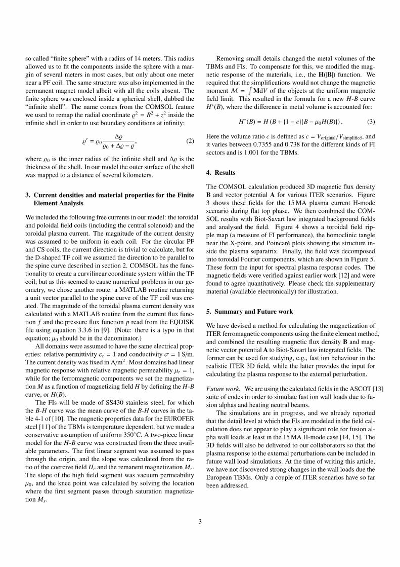
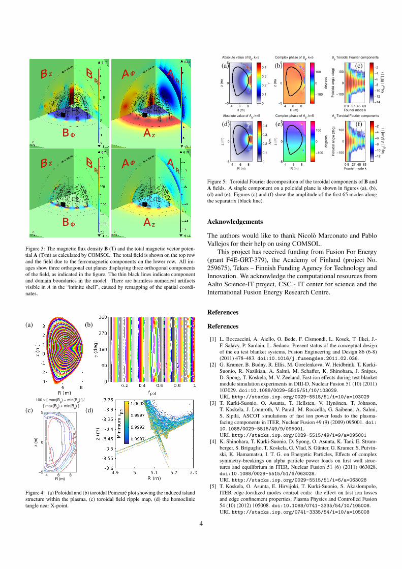
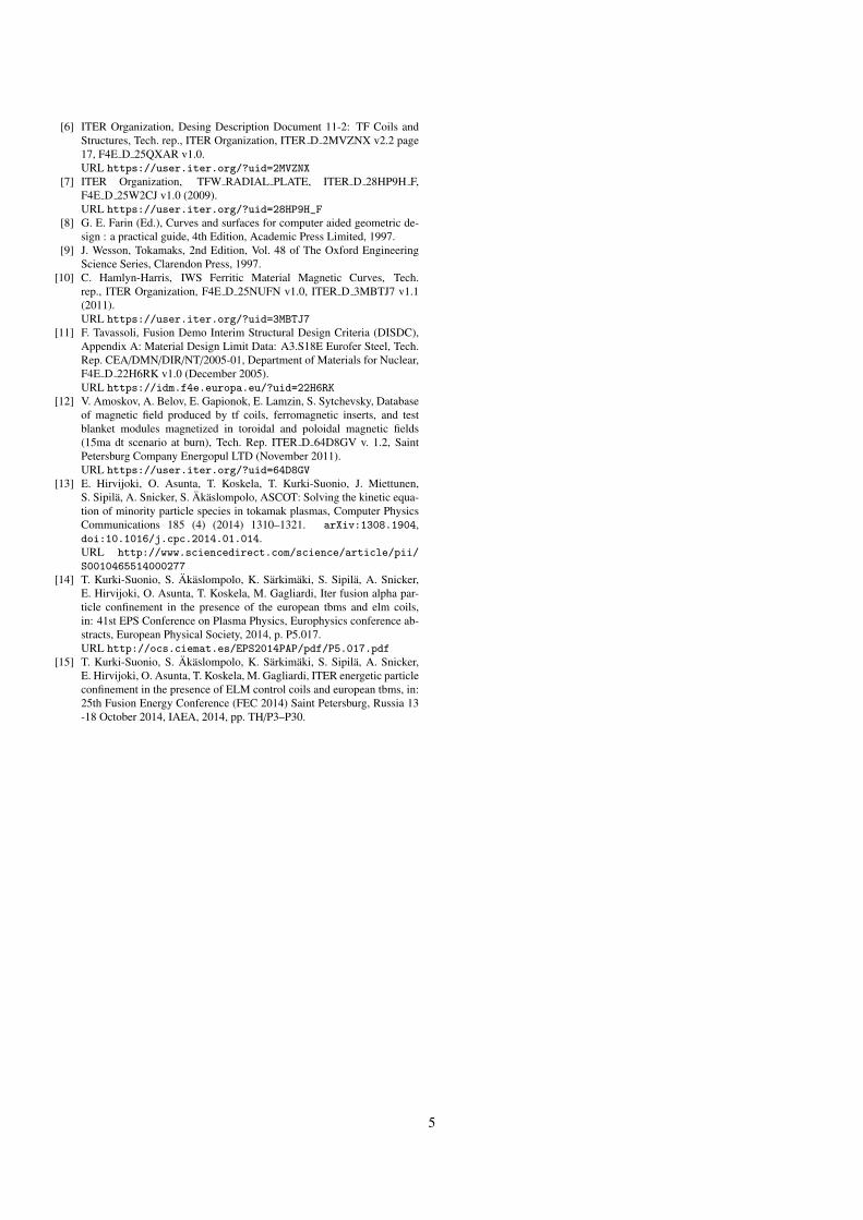
The COMSOL calculation produced 3D magnetic flux densityB and vector potential A for various ITER scenarios. Figure3 shows these fields for the 15 MA plasma current H-modescenario during flat top phase. We then combined the COM-SOL results with Biot-Savart law integrated background fieldsand analysed the field. Figure 4 shows a toroidal field rip-ple map (a measure of FI performance), the homoclinic tanglenear the X-point, and Poincare plots showing the structure in-side the plasma separatrix. Finally, the field was decomposedinto toroidal Fourier components, which are shown in Figure 5.These form the input for spectral plasma response codes. Themagnetic fields were verified against earlier work [12] and werefound to agree quantitatively. Please check the supplementarymaterial (available electronically) for illustration.
5. Summary and Future work
We have devised a method for calculating the magnetization ofITER ferromagnetic components using the finite element method,and combined the resulting magnetic flux density B and mag-netic vector potential A to Biot-Savart law integrated fields. Theformer can be used for studying, e.g., fast ion behaviour in therealistic ITER 3D field, while the latter provides the input forcalculating the plasma response to the external perturbation.
Future work. We are using the calculated fields in the ASCOT [13]suite of codes in order to simulate fast ion wall loads due to fu-sion alphas and heating neutral beams.
The simulations are in progress, and we already reportedthat the detail level at which the FIs are modeled in the field cal-culation does not appear to play a significant role for fusion al-pha wall loads at least in the 15 MA H-mode case [14, 15]. The3D fields will also be delivered to our collaborators so that theplasma response to the external perturbations can be included infuture wall load simulations. At the time of writing this article,we have not discovered strong changes in the wall loads due theEuropean TBMs. Only a couple of ITER scenarios have so farbeen addressed.
3
BΦ
B
BRBz R =
14 m
Az
A
ARAΦ R =
14 m
BΦ
B
BRBz R =
14 m
Az
A
ARAΦ R =
14 m
Figure 3: The magnetic flux density B (T) and the total magnetic vector poten-tial A (T/m) as calculated by COMSOL. The total field is shown on the top rowand the field due to the ferromagnetic components on the lower row. All im-ages show three orthogonal cut planes displaying three orthogonal componentsof the field, as indicated in the figure. The thin black lines indicate componentand domain boundaries in the model. There are harmless numerical artifactsvisible in A in the “infinite shell”, caused by remapping of the spatial coordi-nates.
(a) (b)
(c)
0.01
0.0
1
0.0
5
0.05
0.05
0.0
5
0.05
0.05
0.1
0.1
0.1
0.1
0.1
0.10.1
0.5 0.5
0.5
0.5
0.5
0.50.5
1 1
1
1
1
11
2
22
2
2
2
25
5
5
5 5
5
5
5
5
5
R (m)
z (
m)
100 × [ max(Bφ) − min(B
φ) ] /
[ max(Bφ) + min(B
φ) ]
4 6 8−5
0
5 (d)
Figure 4: (a) Poloidal and (b) toroidal Poincare plot showing the induced islandstructure within the plasma, (c) toroidal field ripple map, (d) the homoclinictangle near X-point.
(a)
4 6 8−5
0
5
Absolute value of Bφ, k=5
R (m)
z (
m)
T
0
0.1
0.2
0.3
0.4 (b)
4 6 8−5
0
5
Complex phase of Bφ, k=5
R (m)
z (
m)
degre
es
−100
0
100
0 9 27 45 63
−100
0
100
Fourier mode k
Polo
idal angle
(deg)
Bφ Toroidal Fourier components
log
10(
| B
[T] | )
−14
−12
−10
−8
−6
−4
−2(c)
(d)
4 6 8−5
0
5
Absolute value of Aφ, k=5
R (m)
z (
m)
A/m
0
0.1
0.2
0.3
0.4 (e)
4 6 8−5
0
5
Complex phase of Aφ, k=5
R (m)
z (
m)
degre
es
−100
0
100
0 9 27 45 63
−100
0
100
Fourier mode k
Polo
idal angle
(deg)
Aφ Toroidal Fourier components
log
10(
| A
[A
/m] | )
−12
−10
−8
−6
−4
−2(f)
Figure 5: Toroidal Fourier decomposition of the toroidal components of B andA fields. A single component on a poloidal plane is shown in figures (a), (b),(d) and (e). Figures (c) and (f) show the amplitude of the first 65 modes alongthe separatrix (black line).
Acknowledgements
The authors would like to thank Nicolo Marconato and PabloVallejos for their help on using COMSOL.
This project has received funding from Fusion For Energy(grant F4E-GRT-379), the Academy of Finland (project No.259675), Tekes – Finnish Funding Agency for Technology andInnovation. We acknowledge the computational resources fromAalto Science-IT project, CSC - IT center for science and theInternational Fusion Energy Research Centre.
References
References
[1] L. Boccaccini, A. Aiello, O. Bede, F. Cismondi, L. Kosek, T. Ilkei, J.-F. Salavy, P. Sardain, L. Sedano, Present status of the conceptual designof the eu test blanket systems, Fusion Engineering and Design 86 (6-8)(2011) 478–483. doi:10.1016/j.fusengdes.2011.02.036.
[2] G. Kramer, B. Budny, R. Ellis, M. Gorelenkova, W. Heidbrink, T. Kurki-Suonio, R. Nazikian, A. Salmi, M. Schaffer, K. Shinohara, J. Snipes,D. Spong, T. Koskela, M. V. Zeeland, Fast-ion effects during test blanketmodule simulation experiments in DIII-D, Nuclear Fusion 51 (10) (2011)103029. doi:10.1088/0029-5515/51/10/103029.URL http://stacks.iop.org/0029-5515/51/i=10/a=103029
[3] T. Kurki-Suonio, O. Asunta, T. Hellsten, V. Hynonen, T. Johnson,T. Koskela, J. Lonnroth, V. Parail, M. Roccella, G. Saibene, A. Salmi,S. Sipila, ASCOT simulations of fast ion power loads to the plasma-facing components in ITER, Nuclear Fusion 49 (9) (2009) 095001. doi:10.1088/0029-5515/49/9/095001.URL http://stacks.iop.org/0029-5515/49/i=9/a=095001
[4] K. Shinohara, T. Kurki-Suonio, D. Spong, O. Asunta, K. Tani, E. Strum-berger, S. Briguglio, T. Koskela, G. Vlad, S. Gunter, G. Kramer, S. Putvin-ski, K. Hamamatsu, I. T. G. on Energetic Particles, Effects of complexsymmetry-breakings on alpha particle power loads on first wall struc-tures and equilibrium in ITER, Nuclear Fusion 51 (6) (2011) 063028.doi:10.1088/0029-5515/51/6/063028.URL http://stacks.iop.org/0029-5515/51/i=6/a=063028
[5] T. Koskela, O. Asunta, E. Hirvijoki, T. Kurki-Suonio, S. Akaslompolo,ITER edge-localized modes control coils: the effect on fast ion lossesand edge confinement properties, Plasma Physics and Controlled Fusion54 (10) (2012) 105008. doi:10.1088/0741-3335/54/10/105008.URL http://stacks.iop.org/0741-3335/54/i=10/a=105008
4
[6] ITER Organization, Desing Description Document 11-2: TF Coils andStructures, Tech. rep., ITER Organization, ITER D 2MVZNX v2.2 page17, F4E D 25QXAR v1.0.URL https://user.iter.org/?uid=2MVZNX
[7] ITER Organization, TFW RADIAL PLATE, ITER D 28HP9H F,F4E D 25W2CJ v1.0 (2009).URL https://user.iter.org/?uid=28HP9H_F
[8] G. E. Farin (Ed.), Curves and surfaces for computer aided geometric de-sign : a practical guide, 4th Edition, Academic Press Limited, 1997.
[9] J. Wesson, Tokamaks, 2nd Edition, Vol. 48 of The Oxford EngineeringScience Series, Clarendon Press, 1997.
[10] C. Hamlyn-Harris, IWS Ferritic Material Magnetic Curves, Tech.rep., ITER Organization, F4E D 25NUFN v1.0, ITER D 3MBTJ7 v1.1(2011).URL https://user.iter.org/?uid=3MBTJ7
[11] F. Tavassoli, Fusion Demo Interim Structural Design Criteria (DISDC),Appendix A: Material Design Limit Data: A3.S18E Eurofer Steel, Tech.Rep. CEA/DMN/DIR/NT/2005-01, Department of Materials for Nuclear,F4E D 22H6RK v1.0 (December 2005).URL https://idm.f4e.europa.eu/?uid=22H6RK
[12] V. Amoskov, A. Belov, E. Gapionok, E. Lamzin, S. Sytchevsky, Databaseof magnetic field produced by tf coils, ferromagnetic inserts, and testblanket modules magnetized in toroidal and poloidal magnetic fields(15ma dt scenario at burn), Tech. Rep. ITER D 64D8GV v. 1.2, SaintPetersburg Company Energopul LTD (November 2011).URL https://user.iter.org/?uid=64D8GV
[13] E. Hirvijoki, O. Asunta, T. Koskela, T. Kurki-Suonio, J. Miettunen,S. Sipila, A. Snicker, S. Akaslompolo, ASCOT: Solving the kinetic equa-tion of minority particle species in tokamak plasmas, Computer PhysicsCommunications 185 (4) (2014) 1310–1321. arXiv:1308.1904,doi:10.1016/j.cpc.2014.01.014.URL http://www.sciencedirect.com/science/article/pii/
S0010465514000277
[14] T. Kurki-Suonio, S. Akaslompolo, K. Sarkimaki, S. Sipila, A. Snicker,E. Hirvijoki, O. Asunta, T. Koskela, M. Gagliardi, Iter fusion alpha par-ticle confinement in the presence of the european tbms and elm coils,in: 41st EPS Conference on Plasma Physics, Europhysics conference ab-stracts, European Physical Society, 2014, p. P5.017.URL http://ocs.ciemat.es/EPS2014PAP/pdf/P5.017.pdf
[15] T. Kurki-Suonio, S. Akaslompolo, K. Sarkimaki, S. Sipila, A. Snicker,E. Hirvijoki, O. Asunta, T. Koskela, M. Gagliardi, ITER energetic particleconfinement in the presence of ELM control coils and european tbms, in:25th Fusion Energy Conference (FEC 2014) Saint Petersburg, Russia 13-18 October 2014, IAEA, 2014, pp. TH/P3–P30.
5