Calculating the Uncertainty of a

Structure from Motion (SfM) Model, Cadman Quarry, Monroe, Washington

Tait S Russell

A report prepared in partial fulfillment of

the requirements for the degree of

Master of Sciences

Earth and Space Sciences: Applied Geosciences

University of Washington

March 2016

Project Mentor:

Dr. Andrew Ritchie

Internship Coordinator:

Kathy Troost

Reading Committee:

Dr. Juliet Crider

Dr. Steven Walters

MESSAGe Technical Report Number: 030

i

©Copyright 2016

Tait S Russell

ii

Abstract

Structure from Motion (SfM) is a new form of photogrammetry that automates the rendering of

georeferenced 3D models of objects using digital photographs and independently surveyed

Ground Control Points (GCPs). This project seeks to quantify the error found in Digital

Elevation Models (DEMs) produced using SfM. I modeled a rockslide found at the Cadman

Quarry (Monroe, Washington) because the surface is vegetation-free, which is ideal for SfM and

Terrestrial LiDAR Scanner (TLS) surveys. By using SfM, TLS, and GPS positioning at the same

time, I attempted to find the deviation in the SfM model from the TLS model and GPS points.

Using the deviation, I found the Root-Mean-Square Error (RMSE) between the SfM DEM and

GPS positions. The RMSE of the SfM model when compared to surveyed GPS points is 17cm. I

propagated the uncertainty of the GPS points with the RMSE of the SfM model to find the

uncertainty of the SfM model compared to the NAD 1984 datum. The uncertainty of the SfM

model compared to the NAD 1984 is 27cm. This study did not produce a model from the TLS

that had sufficient resolution on horizontal surfaces to compare to surveyed GPS points.

iii

Table of Contents

List of Figures ................................................................................................................................ iv

List of Tables ................................................................................................................................. iv

Acknowledgements ......................................................................................................................... v

1.0 Introduction ............................................................................................................................... 1

2.0 Background ............................................................................................................................... 1

2.1 Prior Work ............................................................................................................................. 1

2.2 Study Site .............................................................................................................................. 3

3.0 Methods..................................................................................................................................... 3

3.1 Making GCP Targets ............................................................................................................. 3

3.2 Placing and Measuring GCP Targets .................................................................................... 4

3.3 UAV SfM Survey .................................................................................................................. 5

3.4 TLS Survey ........................................................................................................................... 6

3.5 Post-Processing Aerial Photographs ..................................................................................... 7

3.6 Creating SfM Model.............................................................................................................. 7

3.7 Processing TLS Data ............................................................................................................. 8

3.8 Measuring SfM RMSE .......................................................................................................... 9

3.9 Measuring TLS RMSE ........................................................................................................ 10

4.0 Results ..................................................................................................................................... 10

4.1 Trimble GCPs ...................................................................................................................... 10

4.2 UAV SfM ............................................................................................................................ 10

4.3 TLS ...................................................................................................................................... 10

5.0 Discussion ............................................................................................................................... 11

5.1 Trimble GCPs ...................................................................................................................... 11

5.2 UAV SfM ............................................................................................................................ 12

5.3 TLS ...................................................................................................................................... 12

6.0 Conclusions ............................................................................................................................. 13

6.1 Trimble GPS ........................................................................................................................ 13

6.2 UAV SfM ............................................................................................................................ 13

6.3 TLS ...................................................................................................................................... 13

7.0 Recommendations ................................................................................................................... 14

7.1 Trimble GCPs ...................................................................................................................... 14

7.2 UAV SfM ............................................................................................................................ 14

7.3 TLS ...................................................................................................................................... 15

8.0 References ............................................................................................................................... 16

Appendix A .....................................................................................................................................A

Appendix B ..................................................................................................................................... B

iv

List of Figures

Figure 1: Washington Site Map .................................................................................................... 18

Figure 2: Seattle Site Map............................................................................................................. 19

Figure 3: Local Site Map of Cadman Quarry ............................................................................... 20

Figure 4: Aerial Photograph of GCP Target ................................................................................. 21

Figure 5: SfM Orthophoto with GCP Locations ........................................................................... 22

Figure 6: General “Lawnmower” Flight Path ............................................................................... 23

Figure 7: TLS Scanning Locations ............................................................................................... 24

Figure 8: SfM DEM Over SfM Hillshade..................................................................................... 25

Figure 9: TLS Tie-Points .............................................................................................................. 26

Figure 10: TLS Point Cloud .......................................................................................................... 27

Figure 11: TLS Mesh .................................................................................................................... 28

List of Tables

Table 1: Differential Processing Base Stations ............................................................................. 29

Table 2: GCP Data ........................................................................................................................ 30

Table 3: RMSE Calculations ........................................................................................................ 31

v

Acknowledgements

I would like to start by thanking Dr. Andrew Ritchie for mentoring me during my MESSAGe

project. I would also like to thank Kathy Troost for helping me develop my project and helping

me acquire some of the equipment used during my project. Also, thank you Dr. Steven Walters

and Dr. Juliet Crider for being on my reading committee for this project. Devin Bedard took the

time to come with me and help during my survey, so I would like to thank him for helping me.

While not directly involved with this study, I would like to thank David Shean for mentoring me

on my first Structure from Motion project, which gave me the skills needed to conduct this study.

Finally, I would like to thank Tom Russell and Krista Russell for providing the funding I needed.

1

1.0 Introduction

Geospatial data is needed for military, scientific, and industry uses. Remote sensing is a major

method of acquiring geospatial data. It is able to provide continuous-coverage geospatial data

more easily and cheaply than in-person field methods that provide sparse point data. Geologic

hazard mitigation relies greatly on precise and accurate geospatial data. For example, Digital

Elevation Models (DEMs) can be used to model retreating bluffs, slope failures, and other forms

of land movement that can be hazardous.

Structure from Motion (SfM) is a new and relatively inexpensive form of remote sensing. It is

able to produce DEMs with cm-scale resolution for a small fraction of the cost of Light

Detection and Ranging (LiDAR). Developing a more inexpensive form of remote sensing will

allow for more geospatial data collection. However, because the technique is relatively new,

there are only a few published studies that address the accuracy of landform models produced

with SfM.

My project seeks to quantify the error found in DEMs derived from SfM methodology. I

modeled a rockslide found at the Cadman Quarry (Monroe, Washington) because the surface was

vegetation-free, which is ideal for SfM and TLS (Terrestrial LiDAR Scanner) surveys. See

Figure 1, Figure 2, and Figure 3 for the site location. By using SfM, TLS, and GPS positioning at

the same time, I attempted to find the deviation in the SfM model from the TLS model and GPS

points. I then propagated the deviation with the accuracy of the GPS points to find the

uncertainty of the SfM model.

2.0 Background

2.1 Prior Work

Unmanned Aerial Vehicles (UAVs) with digital cameras can map landslides quickly and with

high precision (Niethammer et al., 2012). UAVs are also known as sUAVs (small Unmanned

Aerial Vehicles), UASs (Unmanned Aerial Systems), sUASs (small Unmanned Aerial Systems),

or simply “drones”. According to Neithammer et al. (2012), photogrammetry experiments using

UAV platforms were started by Prybilla and Wester-Ebbinghaus in 1979. Also according to

Neithammer et al. (2012), the first high-resolution Digital Terrain Model (DTM) using

autonomous UAVs was created by Eisenbeiss et al. in 2005.

Niethammer et al. (2012) surveyed the Super-Sauze landslide using UAVs. They created an

orthographic image with 4cm resolution and Digital Terrain Models (DTMs) with between 3cm

and 8cm resolution (depending on flight heights between 100m and 250m) (Niethammer et al.,

2012). The UAV-photogrammetry-derived DTM, when compared to their TLS scan, had a Root-

2

Mean-Square Error (RMSE) of 31cm in the vertical direction (Niethammer et al., 2012). When

compared to their GCPs (Ground Control Points), the errors were 7.9cm in the x-direction, 7.9cm

in the y-direction, and 18.5cm in the vertical direction (Niethammer et al., 2012). The errors are

considered high and are due to the vegetation obscuring the ground surface (Niethammer et al.,

2012).

Other studies have shown some statistical information regarding the resolution and accuracy of

UAV-photogrammetry-derived DTMs. Chander et al. (2002) created a DTM with 20cm

resolution and a RMSE of 4.5cm (Chander et al., 2002). Levine et al. (2014) created DTMs with

resolutions between 5cm and 10cm, but no accuracy information was available in the published

abstract (Levine et al., 2014). Westboy et al. (2012) found that 100% of the UAV-

photogrammetry-derived DTM cells differ from a TLS scan within +/-50cm on a non-vegetated

surface, but no RMSE was reported. Russell et al. (2014) created a DTM of a glacier terminus

with 7cm resolution and a RMSE of 40cm (estimated using Agisoft PhotoScan Pro software after

construction of the DTM).

In 2012, Dr. Andrew Ritchie developed an airplane-mounted camera system to collect aerial

imagery of the Elwha River and Elwha Delta (Andrew Ritchie, National Parks Service, written

communication, 2015). He uses the photographs to develop SfM models of the Elwha with an

accuracy of +/-20cm relative to LiDAR scans (Andrew Ritchie, National Parks Service, written

communication, 2015). Using the models, Dr. Ritchie can calculate sediment erosion and

deposition in near-real time (Andrew Ritchie, National Parks Service, written communication,

2015). Since he began in 2012, he has run about 80 SfM flights over the Elwha (Andrew Ritchie,

National Parks Service, written communication, 2015).

The work of Lane et al. (2000) and Micheletti et al. (2015) provides useful information on

gathering photographs using UAVs for the purpose of photogrammetry. Lane et al. (2000) found

that UAV-photogrammetry-derived DTM accuracy is limited by image scale and scanning

density. Micheletti et al. (2015) provides a list of important factors to consider when acquiring

the photographs:

It is better to collect images from multiple altitudes.

Photographing the whole site in a few images, then moving in closer for detail is

best.

Using a flash can change the lighting conditions, which makes it harder for SfM

software to reconstruct the area, so no flash is best.

Consistent lighting is best.

It is also best to collect photographs from as many positions as possible.

The more images, the more precise and accurate the model will be.

The survey area should also be static.

3

There will be issues in areas that have high transmissivity, high reflectivity,

and/or are highly homogenous.

2.2 Study Site

Cadman Quarry is located along Highway 203 about 3 miles south of Monroe, WA. The location

of the quarry was over-run by the Cordilleran Ice Sheet during the last glaciation. The related

fluvial-glacial rivers deposited sands and gravels, which are mined for construction purposes.

Also, the quarry is within a fault system (Troost, 2015). The fault system brought bedrock near

the surface, which is rarely found near the surface in the Puget Lowlands. The ability to quarry

hard-rock, sands, and gravels within the same site is why Cadman is excavating the area.

Along the east benches of Cadman Quarry, there is a rockslide in one of the hard-rock quarry

bench roads. The rock has fractured nearly vertically, sliding down and away from the scarp,

leaving a large tension crack about 10 meters wide between the rockslide and the scarp. The

rockslide did not have any movement in 2015 (Robby Johnson, Cadman Inc., oral

communication, 2015).

The rockslide at Cadman Quarry was chosen for this study because it is unvegetated. Vegetation

obscures the ground in photographs, resulting in poorer ground coverage and a lower quality

SfM model.

3.0 Methods

3.1 Making GCP Targets

Before conducting the survey, I made thirty Ground Control Point (GCP) targets for both

georeferencing the SfM model and for error checking. See Figure 4. Each target was made by

cutting a square approximately 35cm by 35cm out of a light-blue tarp. I then placed a small,

square piece of orange tape (approximately 4cm by 4cm) in the center of the target to be the

“bullseye” where the GPS measurement was taken. The bright orange is intended to be easily

seen in the collected photographs. In order to differentiate the GCP targets, I taped a large

number on each target using orange tape. I also taped a single stretch of orange tape beneath the

number for orientation (differentiating numbers like “12” and “21”).

4

3.2 Placing and Measuring GCP Targets

The survey was on done January 2nd, 2016. We started at about 11:00am (PST). It was a clear,

sunny day with temperatures around 45 degrees Fahrenheit.

Once in the field, I placed the GCP targets and measured their GPS location. The original plan

was to place GCP targets east, west, north, and south of the sliding bench. However, the bench

east the slide was marked as “do not enter”, so the GCP targets were placed on the next bench

east. Unfortunately, the south side of the bench was completely inaccessible. A total of seventeen

targets were placed around the sliding bench. See Figure 5. GCPs with identifier numbers less

than 20 were placed for georeferencing the SfM model, whereas GCPs with identifiers 20 and

greater were placed for error checking. I placed the modeling-GCPs along the sides of the

benches to better constrain the edges of the benches, whereas I placed the error-checking-GCPs

along the center of the benches to maximize the distance from the modeling-GCPs.

After placing each GCP target, I measured its GPS location using a Trimble Geo 7x with an

external receiver. The Trimble Geo 7x is a GPS receiver/transmitter with a laser range finder. It

is capable of marking GPS positions within 1cm horizontally and 1.5cm vertically when

connected to a real-time base station (Trimble, 2015). I gathered GPS data with the external

receiver until the estimated post-processing accuracy shown on the Trimble read 2cm. To keep

track of which GPS measurement went with which GCP target, I saved the GCP target number in

the comment section of each GPS measurement.

To increase the accuracy of the GCP data, the GPS points collected by the Trimble were run

through GPS Pathfinder Office (v4.00) to apply differential processing corrections. Differential

processing uses GPS information recorded at a stationary GPS base station to remove errors in

the GPS measurements caused by fluctuations in the magnetosphere of the Earth. I used the

following processing steps modified by instructions given by Brian Holmes (University of

Washington: Earth and Space Sciences Department, written communication, 2014). For the

differential processing in GPS Pathfinder Office, I used the “Automatic Carrier and Code

Processing (Recommended)”. I then selected “Use Multiple Base Providers” with default

correction settings. I created a new base provider group and selected three base stations: a

UNAVCO station in Issaquah, WA; a UNAVCO station in Bayview, WA; and a UNAVCO

station in Darrington, WA. See Table 1. I selected these stations because they resulted in the best

estimated accuracy reported by the program after trying every combination of on-line, rated base

stations within 100km. After creating the base provider group, I had the program use the

reference position from the base providers. Finally, I selected the “Sample ESRI Shapefile Set-

Up” as the export (adding position attributes under “Properties”).

5

After the GPS Pathfinder Office program finished processing and exporting the GPS points, I

imported the point data into ArcMap (v.10.2.1.3497). Once imported, I defined the projection

system because the shapefile did not have the projection system defined. I used the WGS 1984

coordinate system, which the Trimble was set to measure coordinates relative to. Finally, I

exported the attribute table of the shapefile as a text file in order to import the GCPs into the SfM

program, Agisoft PhotoScan Pro.

3.3 UAV SfM Survey

To collect the photographs needed for SfM, I flew a DJI Phantom 2 Vision+ (a civilian

recreational drone). I used three DJI Phantom 2 Vision+ rechargeable batteries, with each

allowing for about 15 minutes of flight (a total of about 45 minutes). The drone is equipped with

a 14MP gimbal-stabilized camera.

The Phantom 2 Vision+ is not water resistant at all and cannot be used in wet conditions like

rain, snow, or heavy fog (DJI, 2015). The drone also cannot fly in heavy winds nor under zero

degrees Celsius (DJI, 2015). So, planning a survey date is weather-dependent. Luckily, the

weather was a clear, sunny day with little to no wind during our survey of the quarry.

Because SfM works by using photographs, there must be enough ambient light to capture high-

quality images. The ambient lighting conditions must be unchanging, otherwise SfM programs

cannot find the patterns found between images needed to reconstruct the survey area. The drone

SfM survey took about an hour, so the elevation of the sun changed by several degrees, slightly

changing the shadow lengths and lighting conditions.

Because this study used a drone to acquire the images, Federal Aviation Administration (FAA)

regulations had to be considered. When this survey was conducted on January 2nd, 2016, I flew

under the FAA hobby aircraft guidelines. Along with not being able to use data for profit, this

meant that I had to fly under the following rules (FAA, 2015):

Fly below 400 feet and remain clear of surrounding obstacles.

Keep the aircraft within visual line of sight at all times.

Remain well clear of and do not interfere with manned aircraft operations.

Don't fly within 5 miles of an airport unless you contact the airport and control tower before

flying.

Don't fly near people or stadiums.

Don't fly an aircraft that weighs more than 55 lbs.

Don't be careless or reckless with your unmanned aircraft – you could be fined for

endangering people or other aircraft.

6

I was able to complete the survey without violating the FAA guidelines. Following the

guidelines did not impede the aerial survey in any way.

Prior to flying the drone, I set the camera to automatically adjust its exposure, shutter speed, and

aperture. I also set the camera to take a photograph every 3 seconds (as fast as it can). This

procedure required photos to be captured in JPEG format, because RAW files (which are

typically recommended for SfM) can capture only as fast as one photograph every 30 seconds.

For the first 30 minutes of flight-time, I collected low-altitude photographs of the bench faces. I

did this by pointing the camera on the drone straight down and flying 5-15m above each bench.

For best coverage, I flew in a “lawnmower” pattern. See Figure 6. To increase overlap between

subsequent photographs and to reduce motion blur, I flew very slowly (0.5-1m/s). The amount of

overlap between photographs was unknown during the survey.

For the last 15 minutes of flight-time, I collected high-altitude photographs of the bench faces as

well as photographs of the rock walls. The high-altitude photographs were collected because

Micheletti et al. (2015) recommends acquiring photographs from multiple altitudes. For the high-

altitude photographs, the camera was kept pointed straight down while I flew at a height of about

25m. I flew across the survey area and back once at speeds less than 1m/s. Lastly, I collected

photographs of the rock walls in the survey area. To do this, I set the camera on the drone to

point forward while I flew slowly (0.5-1m/s) along each wall. I flew at a height about halfway up

each wall, and back away from the wall far enough for the vertical extent of each wall to be

captured in each photograph.

3.4 TLS Survey

A Riegl VZ-4000 Terrestrial LiDAR System (TLS) was used to collect the LiDAR data. The

TLS is capable of scanning from up to 4km away with an angular resolution as small as 0.0005

degrees, and a precision of 1cm at 150m (Riegl, 2015). So, the TLS can be used for very high-

resolution modeling.

Three locations were selected from which to scan the quarry with TLS: one north of the sliding

bench, one south of the slide, and one west of the slide. The locations were selected because they

were the highest elevations locations from which to scan the rockslide with the TLS. The three

scan locations are shown in Figure 7.

At each scanning location, we placed four of the TLS reflector targets around the TLS, 5-15m

away at slightly different elevations, to enable the TLS system to correctly orient and

georeference itself. For each of the three scans, we set the TLS to do a 360 degree panorama

scan at 50kHz with an angular resolution of 0.08 degrees. We also set the TLS to collect

photographs for each scan, which allows for colorization of the TLS model. By draping the

7

photographs collected by the TLS over the point cloud model, the survey area can have a

colorized texture, which is needed to locate the GCPs.

3.5 Post-Processing Aerial Photographs

The GPS information stored as geotags in the photographs collected by the drone is not of

sufficient accuracy to use in SfM. When loaded into Agisoft PhotoScan Pro, the photographs

were grouped together in a perfect grid pattern, which indicates the GPS information in the

geotags is not accurate. The altitudes were all recorded as 0m because the DJI Phantom 2

Vision+ does not store altitude information in the geotags. If the geotags were used, Agisoft

PhotoScan Pro would have trouble properly aligning the photographs when the geotags indicate

a false position.

These geotags must be removed from the metadata for each photo; otherwise, the SfM software

(Agisoft PhotoScan Pro) may incorrectly place and align the camera positions. To quickly and

easily remove the GPS data from all of the photographs at once, I used an open-source script

program called “EXIFtool” (Harvey, 2016). Using the command “exiftool -gps:all= -

xmp:geotag= DJI*.jpg”, I was able to remove the geotags from all of the photographs collected

by the drone (Ask Ubuntu, 2013).

3.6 Creating SfM Model

The computer I used to run the SfM software was a Dell Precision Tower 7000 Series. It uses

two Intel Xeon hyper-threading 6-core processors (a total of 12 cores that simulate 24 by hyper-

threading). The computer is also equipped with two graphics cards: a GeForce GTX 780 Ti and a

Quadro 4000. The computer has 64GB of RAM.

The program I used for SfM modeling on this project was Agisoft PhotoScan Pro (v.1.2.3). I

started by creating a new project and loading the post-processed photographs. Next, I created the

sparse point cloud by aligning the photographs using the “high” accuracy setting for the greatest

accuracy. The sparse cloud is a point cloud of the features/patterns found between the aligned

photographs. For the sparse cloud alignment, I set the photograph selection to “generic” because

the photographs no longer have geotags (Agisoft, 2016). Also, I increased the maximum number

of points (features/patterns detected by Agisoft PhotoScan Pro in each photograph) to 400,000

and the maximum number of ties (corresponding features/patterns detected in other photographs)

to 10,000. I did this because the console processing report showed that the program was finding

more points than the default maximums of 40,000 points and 1,000 ties. After the sparse cloud

was created, I deleted the extraneous points that were generated outside the survey area to reduce

the processing time of generating the dense point cloud.

8

Next, I imported the GCPs as the markers into the program using the attribute table exported

from ArcMap. I then found and placed the GCP marker on the target bullseye of each GCP target

placed for georeferencing (GCP identifiers less than 20) in three photographs. That allowed the

program to estimate the placement of the GCP markers in the rest of the photographs. I then

adjusted and placed the markers. Markers were not placed in photographs that were taken at

high-altitude or where the GCP is visible only along the periphery of the photograph. After

placing the GCPs meant for georeferencing the model, I had the program optimize the estimated

camera lens distortion. With these settings in place, I updated the photograph alignments,

estimated camera positions, and sparse cloud.

After finishing the sparse point cloud, I generated a dense point cloud. The dense point cloud is a

denser point cloud created based on the estimated camera positions (Agisoft, 2016). The program

calculates depth information for each photograph to create the dense point cloud (Agisoft, 2016).

I set the cloud density to “medium” because higher settings can over-interpolate and create noisy

surfaces (David Shean, University of Washington: Earth and Space Sciences Department, oral

communication, 2014). Also, I set the depth filtering to “mild” because there was no vegetation

and the survey area was full of angular, jagged surfaces that I do not want to have smoothed out.

Once the dense point cloud was generated, I deleted poorly modeled points generated in the

periphery of the survey area.

With the model finished, I built a DEM using the dense point cloud. I then exported a

georeferenced TIFF file for the DEM using the WGS 1984 State Plane Washington Zone 10N

(meters) coordinate system because it is easier to measure the error in ArcMap using meters than

it is using degrees. I used the default pixel size of about 4.0cm suggested by the program. I also

had the program estimate the bounding area, which writes the bounding latitude and longitude

information into the metadata. See Figure 8.

Next, I generated an orthophoto based on the DEM surface and using the “average” texture

setting. See Figure 5. Like the DEM, I chose to export the orthophoto as a georeferenced TIFF

file using the WGS 1984 State Plane Washington Zone 10N (meters) coordinate system. Again, I

used the default pixel size suggested by the program (about 1.0cm) and allowed the program to

estimate the bounding area.

3.7 Processing TLS Data

First, I opened the project file saved during the survey in RiScan Pro (v.2.0.3). Next, I loaded the

point cloud of each scan separately. I then found objects in the survey area that could be used as

tie-points between the three scans. See Figure 9. Using seven tie-points, the program was able to

coregister the three scans. With the three scans coregistered, I converted the point cloud into an

object. Finally, I created a mesh surface using the object. The mesh was generated using an

9

oblique view (about 270 degrees azimuth and 45 degrees elevation) because the mesh generates

relative to the viewing angle, and the mesh was required on both the bench faces and walls.

3.8 Measuring SfM RMSE

The RMSE is a widely used single-value aspatial statistic indicating the deviation of estimated

values within a data set from their true values (Erdogan, 2009). By squaring the difference

between a data point and its true value, more weight is given to larger deviations. It has been

used for many geospatial studies including landslides and remote sensing methodology

comparisons (Erdogan, 2009; Hofierka et al., 2013; Sharma et al., 2010; Tan et al., 2014;

Travelletti et al., 2012; Yao et al., 2014).

In ArcMap, I loaded in the GCPs defined by GPS data, the SfM orthophoto, and the SfM DEM.

Using the measurement tool in ArcMap, I measured the horizontal difference between the GCPs

and their corresponding target generated in the SfM orthophoto. To measure the elevation

difference, I sampled the elevation value in the DEM cell where the corresponding GCP target

was generated. I calculated the total offset between the Trimble-measured GCPs and the SfM-

generated GCPs using Equation 1. I then calculated the RMSE using Equation 2.

Equation 1: d = (h2 + e2)0.5

d is total offset distance.

h is horizontal offset.

e is elevation difference.

Equation 2: RMSE = √∑ 𝑑𝑖

2𝑛𝑖=0

𝑛

2

RMSE is the root-mean-square error.

di is the total offset of each GCP.

n is the number of GCPs used.

To know the uncertainty of the SfM model compared to the NAD 1984 datum, I propagated the

uncertainty of the GCP measurements with the RMSE of the SfM model using Equation 3

(Shilpakar et al., 2016).

Equation 3: u = (RMSE2 + h2 + v2)0.5

u is the uncertainty of the SfM model.

RMSE is the root-mean-square error.

h is the horizontal accuracy of the GCPs.

v is the vertical accuracy of the GCPs.

10

3.9 Measuring TLS RMSE

Despite scanning from the highest elevation areas we could reach with the TLS, the survey did

not collect enough points on the bench surfaces for a continuous mesh to be generated. Also, we

were not able to collect any points in the tension crack at the head of the rockslide. This made it

impossible to measure the TLS error using the GCPs placed on the benches.

4.0 Results

4.1 Trimble GCPs

A total of seventeen GCPs were collected in the survey area. Eleven of the GCPs were placed for

georeferencing the SfM model and six for error checking. The vertical and horizontal accuracy

of the GCPs are within 15cm. See Table 2.

4.2 UAV SfM

A total of 786 aerial photographs were collected by the drone to generate the SfM model. Agisoft

PhotoScan Pro reported all locations within the survey area had at least nine overlapping images.

Agisoft PhotoScan Pro found 6.15×105 points for the sparse cloud within the survey area and

3.60×107 points for the dense cloud. With that data, the program produced a DEM with a

resolution of 4.0cm and an orthophoto resolution of 1.0cm. It took about 24 hours of processing

time to generate the model and export the results.

Using ArcMap, I found that the RMSE of the SfM model compared to the surveyed GCPs is

17cm. See Table 3. When combined with the accuracy of the GCPs, the uncertainty of the SfM

model compared to the NAD 1984 datum is 27cm.

4.3 TLS

Three scans were done using the TLS. RiScan Pro reported that the standard deviation of the tie-

points between the three scans was about 33cm, which is higher than the 10cm found when using

reflectors (Coire McCabe, University of Washington: Earth and Space Sciences Department, oral

communication, 2016). With the three scans, a total of 6.55×105 points were collected in the

survey area. Very few points were collected on the bench faces and none in the tension crack of

the slide due to the low elevation of the scan positions and highly oblique angle of scanning.

Hence, modeling of the bench faces and the tension crack was not possible. See Figure 10 and

Figure 11. With gaps on the benches, I could not calculate the RMSE using the surveyed GCPs.

11

5.0 Discussion

The initial goals of this study were to calculate the RMSE of a SfM model compared to both a

TLS model and GPS positions. I collected seventeen GCPs using a Trimble Geo 7x (eleven for

the SfM model and six for error-checking). The GCPs have an accuracy within 15cm both

horizontally and vertically. Using a drone, I collected 786 aerial photographs that I used to create

a SfM model of the survey area. The resulting SfM DEM and orthophoto have resolutions of

4.0cm and 1.0cm, respectively. When compared to the GCPs, the SfM model has a RMSE of

17cm. When compared to the NAD 1984 datum, the SfM model has an uncertainty of 27cm. A

sufficient TLS model was not able to be generated due to occlusions of many of the benches and

the tension crack.

5.1 Trimble GCPs

Accurate measurements for the GCPs by the Trimble were paramount for this project. The

accuracy of the GCPs must be high in order to have an accurate model as well as correctly

estimate the RMSE in the SfM model. For the Trimble to report a real-time estimated horizontal

accuracy of 2 cm, the Trimble had to collect data at each GCP for several minutes (about two to

five). Placing and measuring the GCPs ended up being the most time-consuming part of the

survey. Unfortunately, the in-field estimate of a 2 cm error was optimistic. Even though the

Trimble collected data at each GCP until the post-processing accuracy was estimated to be 2cm,

the errors reported by GPS Pathfinder Office after post-processing were up to 15cm horizontally

and vertically.

I believe the accuracy could be improved if better base stations are used for the differential

processing. For this study, I used three UNAVCO base stations. However, Washington State has

a very accurate base station network (the Washington State Reference Network) that can, in

principle, be used for differential processing. However, differential data is not available for the

day of the survey.

On the benches of the quarry, the rock walls blocked the GPS signals from satellites in the

eastern portion of the sky. In the field, I noticed fewer satellites were being used by the Trimble

for GCPs close to the rock walls. I also noticed that my own body could interfere with the GPS

signals, dropping the number of satellites connected to the Trimble when I stood near the

external receiver.

With a Trimble, the user must be physically able to reach a location to measure the GPS location.

At the quarry, I was unable to place GCPs to the south of the sliding bench because there was no

accessible path to that area, which left the south side of the model barren of GCPs. I was also

unable to place GCPs on the bench directly east of the sliding bench. That area was not permitted

12

for entry due to the danger of another bench failure. Agisoft (2016) recommends complete

coverage of the survey area with GCPs for the highest accuracy.

Finally, correctly placing the GCPs in the locations desired was difficult. The quarry roads had

been changed between the desk review of the site and the survey. With the roads changed, I was

unable to correctly place the GCPs along the entire length of the western bench.

5.2 UAV SfM

Because the SfM model required the GCPs for georeferencing, the accuracy of the GCPs affect

the accuracy of the model. The accuracy of the GCPs was within 15cm horizontally and

vertically, which was substantially larger than the attempted 2cm. With more accurate GCPs, the

accuracy of the SfM model will improve.

The SfM model also relies on digital photographs in order to render the scenery. Low-quality

photographs (blurred, over/under exposed, small sensor chip, low Megapixel, etc.) will degrade

the model. Because the Phantom 2 Vision+ uses a rolling shutter, it is susceptible to blurring if

the drone is moving quickly (Andrew Ritchie, National Parks Service, written communication,

2015). However, I flew at such slow speeds (less than 1m/s) that the rolling shutter should not

have affected the image quality.

Another possible issue with SfM surveying is not knowing what resolution the model will end up

having. It is difficult (if not impossible) to predict what resolution the model will have. This

could lead to either under-developing the model (too low of a resolution) or over-developing the

model (wasting processing time). With most of the processing time automated by Agisoft

PhotoScan Pro, I favored trying to over-develop the model, so critical features that needed to be

modeled were not lost.

5.3 TLS

What most affected the ability of the TLS to scan the survey area was the location from which it

scanned the survey area. The TLS is not capable of aerial surveying, so every part of the survey

area must be viewable from ground positions. This was the limiting factor for our survey of the

quarry. Because of the danger of bench failure, we were not allowed to walk beyond the line of

boulders that stretch along the benches. This prevented us from being able to scan the sliding

bench face from the benches to the north, south, and east. We attempted to scan the bench faces

by scanning from the highest locations accessible. However, we were neither able to collect

enough points on the bench faces to generate a model, nor were we able to collect any points

within the tension crack of the slide.

13

The tie-points used can also be a source of error. The tie-points are needed to coregister the

scans, bringing them together into one model. Tie-points are created by identifying and marking

objects within the scanning area. Because the scans were set to a lower resolution of 0.08

degrees, most of the objects that could be used for tie-points were only partially modeled. This

made it difficult to correctly place the tie-point in the same location in each of the three scans.

The standard deviation of the tie-points was calculated by RiScan Pro to be about 33cm, which is

higher than the 10cm possible when using reflectors (Coire McCabe, University of Washington:

Earth and Space Sciences Department, oral communication, 2016).

6.0 Conclusions

6.1 Trimble GPS

Using a Trimble Geo 7x, I collected seventeen GCPs (eleven for SfM modeling and six for error-

checking). See Figure 5. No GCPs were placed on the bench south of the rockslide due to the

inaccessibility of the southern bench. The GPS data was post-processed using differential

correction. Three UNAVCO base-stations were used for the differential processing. See Table 1.

The post-processed horizontal and vertical accuracy of the GPS data was estimated by GPS

Pathfinder Office to be less than 15cm. See Table 2.

6.2 UAV SfM

Using a drone and SfM, the entire survey area was surveyed aerially. The SfM model created

using the aerial photographs was free of occlusions (gaps). The model resulted in an extremely

high-resolution DEM and orthophoto (4.0cm and 1.0cm, respectively). See Figure 5 and Figure

8. However, the RMSE found in the SfM products was calculated to be 17cm. See Table 3. The

uncertainty is 27cm compared to the NAD 1984 datum. I believe the uncertainty of the SfM

products are so large in comparison to their resolution because of the poor quality of the GCPs.

Had I placed more GCPs and measured them more accurately, I believe the RMSE and

uncertainty could be much smaller because Agisoft (2016) recommends complete coverage of

the survey area with GCPs.

6.3 TLS

Due to the data gaps along the bench faces and within tension crack at the head of the slide, the

RMSE of the TLS could not be found. Had we been able to scan from higher elevations, we may

have been able to scan the bench faces. However, we still would not have been able to scan

within the tension crack of the slide.

The most limiting factor for the TLS in this study is that it was constrained to scanning from the

surface of the ground. The TLS cannot scan horizontal surfaces at elevations higher than itself.

14

This can be a problem when attempting to scan areas with horizontal surfaces and high relief, or

when there is limited access to locations from which to scan the area.

A TLS would be useful for scanning areas with minimally complex geometry. The less complex

the geometry of the survey area, the few scanning locations will need to be used to eliminate

occlusions. The rockslide at Cadman Quarry was too angular and complex to scan from the

ground alone – aerial LiDAR would be needed for complete coverage. Formations like landslide

scarps, bluffs, and road cuts would be ideal for TLS surveys.

7.0 Recommendations

7.1 Trimble GCPs

Because the estimated post-processing accuracy displayed in-field by the Trimble Geo 7x is not

accurate, I highly recommend allowing the Trimble to continue collecting GPS data at each

location well after it shows the post-processing accuracy desired. I also recommend connecting

the Trimble to a hot-spot internet connection, so that it can apply the differential correction in-

field.

The targets that I used for this study worked, but they could be improved. In most of the

photographs, it was difficult to determine where the bullseye was in each GCP. Using the same

quality camera that is attached to the Phantom 2 Vision+, I would recommend using larger

targets, each with a larger identification number and bullseye. Another option would be to use

the coded targets that can be generated and printed from Agisoft PhotoScan Pro. With large

enough coded targets and/or a good enough aerial camera, Agisoft PhotoScan Pro can

automatically detect the GCPs. This would eliminate the need to manually find each GCP within

several photographs.

While not always physically possible, it is best to place GCPs around the entire survey area.

Agisoft (2016) recommends this for maximum accuracy of the SfM model.

7.2 UAV SfM

While the DJI Phantom 2 Vision+ is easy to use and ready out-of-the-box, I recommend using a

drone with a better camera and, if possible, use one that is also waterproof. Even though I flew at

heights less than 15m for the high-quality images, it was difficult to resolve the information on

each GCP in many of the photographs. It would be better to use a camera with a larger sensor,

higher Megapixels, uses a global shutter (instead of a rolling shutter), and is capable of using a

RAW file type for continuous photographing (instead of JPEG). Unlike JPEG, RAW does not

compress the image data. Compressed images can reduce the quality of SfM models.

Furthermore, with a drone that is waterproof, it is possible to survey under wet conditions.

15

Finally, it would be beneficial to use a drone and camera mount that is capable of correctly

geotagging the aerial photographs. While geotags may not improve the accuracy or resolution of

the SfM model, they will reduce the processing time Agisoft PhotoScan Pro needs to align the

photographs and create the sparse point cloud (Andrew Ritchie, National Parks Service, oral

communication, 2016).

As mentioned earlier, the GCP accuracy could be improved by allowing the Trimble to continue

collecting data after it shows the desired post-processing accuracy. Increasing the accuracy of the

GCPs will increase the accuracy of the SfM model. Also, placing more GCPs, especially on the

south side (where none were able to be placed during our survey), would increase the accuracy

of the SfM model (Agisoft, 2016). However, I do not know how much the accuracy would

increase by doing so.

The “lawnmower” flight pattern worked well. However, more flight time would be useful. With

a fourth or fifth battery, more photographs could have been collected around the perimeter of the

site, where fewer points were found for the sparse and dense point clouds.

I recommend using the same processing steps that I used in Agisoft PhotoScan Pro. I also

recommend using the same exporting steps that I used.

7.3 TLS

I recommend carefully considering what surfaces need to be scanned, then estimate scanning

locations that will be able to view those surfaces. Be sure to pick scanning positions that are high

enough to view the surfaces. It may be possible to see the surface from the scanning position

when in the field, but if the surface is highly oblique from that scanning position, very few points

may be collected on that surface. I recommend doing a quick, low-resolution scan of the area

first, checking the point cloud to see if enough points will be collected from that position. Once a

good position has been determined, then scan using higher-resolution settings.

Instead of using scanned objects within the study area as tie-points, I recommend using the TLS

reflector targets. By placing the reflector targets in the study area, they can be used as tie-points.

Because the reflectors return brighter laser pulses than the ground, they are easy to find in

RiScan Pro. This can reduce the standard deviation between tie-points.

16

8.0 References

Agisoft, 2016, Help: PhotoScan Pro (v1.2.3): a Structure from Motion modeling program.

Ask Ubuntu, 2013, How can you delete only GPS metadata from a jpeg file?:

http://askubuntu.com/questions/236455/how-can-you-delete-only-gps-metadata-from-a-

jpeg-file (accessed January 2016).

Chandler, J.H., Ashmore, P., Paola, C., Gooch, M., Varkaris, F., 2002, Monitoring river-channel

change using terrestrial oblique digital imagery and automated digital photogrammetry:

Annals of the Associated of American Geographers, v. 92, no. 1, p. 631-644.

DJI, 2015, Phantom 2 Vision+ User Manual v.1.8 (English):

http://dl.djicdn.com/downloads/phantom_2_vision_plus/en/Phantom_2_Vision_Plus_Use

r_Manual_v1.8_en.pdf.

Erdogan, S., 2009, A comparison of interpolation methods for producing digital elevation models

at the field scale: Earth Surface Processes and Landforms, v. 34, no. 3, p. 366-376.

FAA, 2015, Model Aircraft Oporations: https://www.faa.gov/uas/model_aircraft/ (accessed

January 2016).

Google Earth, 2016, Cadman Quarry, 47o48’56.74”N, 121o57’38.73”W, Landsat June 8th, 2015

(accessed January, 2016).

Google Earth, 2016, Monroe, 47o51’24.11”N, 121o58’04.91”W, Landsat April 9th, 2013

(accessed February, 2016).

Harvey, P., 2016, EXIFTool: a program that modifies the EXIF information within programs:

http://www.sno.phy.queensu.ca/~phil/exiftool/.

Hofierka, J., Gallay, M., Kanuk, J., 2013, Spatial Interpolation of Airborne Laser Scanning Data

with Variable Data Density: Proceedings of the 26th International Cartographic

Conference.

Lane, S.N., James, T.D., Crowell, M.D., 2000, Application of digital photogrammetry to

complex topography for geomorphological research: The Photogrammetric Record, v. 16,

no. 1, p. 793-821.

Levine, N., Ali, K., Chadwick, J., 2014, LIDAR Verses drone: DEM creation, accuracy, and

other issues: Geological Society of America Abstracts with Programs, v. 46, no. 6, p.

297.

Micheletti, N., Chandler, J.H., Lane, S.N., 2015, Structure from Motion (SfM) Photogrammetry:

British Society for Geomorphology, Geomorphological Techniques, Ch. 2, Sec. 2.2,

ISSN 2047-0371.

National Park Service (NPS), 2003, European and Euro-American History: Olympic National

Park, http://www.nps.gov/olym/planyourvisit/upload/Euro-history_printer-friendly.pdf

(accessed October 2015).

National Park Service (NPS), 2015, About US: http://www.nps.gov/aboutus/index.htm (accessed

October 2015).

17

Niethammer, U., James, M.R., Rothmund, S., Travelletti, J., Joswig, W., 2012, UAV-based

remote sensing of the Super Sauze landslide: evaluation and results: Engineering

Geology, v. 128, no. 1, p. 2-11.

Riegl, 2015, Riegle VZ-4000:

http://www.riegl.com/uploads/tx_pxpriegldownloads/DataSheet_VZ-4000_2015-03-

24.pdf (accessed January 2016).

Russell, T., Shean, D., Crider, J., 2014, A high-resolution DEM timeseries to measure glacial

mass balance, dynamics, and variability at Mount Baker, WA USA: Geological Society

of America Abstracts with Programs, v. 46, no. 6, p. 105.

Sharma, A., Tiwari, K. N., and Bhadoria, P. B. S., 2010, Quality assessment of contour

interpolated digital elevation models in a diverse topography: International Journal of

Ecology & Development, v. 15, no. W10, p. 26-42.

Shilpakar, P., Oldow, J. S., Walker, J. D., Whipple, K. X., 2016, Assessment of the uncertainty

budget and image resolution of terrestrial laser scans of geomorphic surfaces: Geosphere,

v. 12, no. 1, p. 281-304.

Tan, Q., Xu, X., 2014, Comparative Analysis of Spatial Interpolation Methods: an Experimental

Study: Sensors & Transducers, v. 165, no. 2, p. 155.

Travelletti, J. and Malet, J.P., 2012, Characterization of the 3D geometry of flow-like landslides:

A methodology based on the integration of heterogeneous multi-source data: Engineering

Geology, v. 128, no. 1, p. 30-48.

Trimble, 2015, Trimble Geo 7x Datasheet:

http://trl.trimble.com/docushare/dsweb/Get/Document-730024/022516-

098A_Geo%207Xw%20Access_DS_US_0415_LR.pdf (accessed February 2016).

Troost, K., 2015, Cadman Quarry: https://canvas.uw.edu/courses/947181/files (accessed

February 2015).

Westoby, M., Brasington, J., Glasser, N., Hambrey, M., Reynolds, J., 2012, ‘Structure-from-

Motion’ photogrammetry: A low-cost, effective tool for geoscience applications:

Geomorphology, v. 179, no. 1, p. 300-314.

Yao, L, Huo, Z., Feng, S., Mao, X., Kang, S., Chen, J., Xu, J., Steenhuis, T.S., 2014, Evaluation

of spatial interpolation methods for groundwater level in an arid inland oasis, northwest

China: Environmental Earth Sciences, v. 71, no. 4, p. 1911-1924.

18

Figure 1: Aerial image showing the location of the Cadman Quarry site in Washington State

(marked by the red star). (Google Earth a, 2016)

19

Figure 2: Aerial image showing the location of the Cadman Quarry site (marked by the red star).

(Google Earth a, 2016)

20

Figure 3: Aerial image of Cadman Quarry (Google Earth b, 2016). The rockslide is shown within

the orange circle.

21

Figure 4: Aerial photograph of GCP #0. The GCP is about 35cm by 35cm.

22

Figure 5: Composite orthophoto of Cadman Quarry derived from the SfM DEM, with GCP

placement around the rockslide study area. A total of seventeen GCPs were placed. The rockslide

and tension crack in the center were well resolved. The resolution is high enough that the safety

boundary boulders around the bench perimeters are also well resolved. Resolution: 1.0cm.

23

Figure 6: General “lawnmower” flight path used for this study.

24

Figure 7: Aerial photograph showing the TLS scanning locations using stars (Google Earth b,

2016). The scanning locations are represented by the green stars.

25

Figure 8: This is a DEM map over a hillshade of the rockslide at Cadman Quarry derived using

SfM. The bench of the rockslide can be seen in blue-green near the center. Resolution: 4.0cm.

26

Figure 9: These images show each tie-point (represented by the red dot within the red circle)

used to coregister the three TLS scans. The dark areas are the benches, whereas the white/grey

areas are the rock walls. The white arrows point north.

27

Figure 10: Coregistered point cloud of the three TLS scans. The black areas are the benches,

whereas the white/blue areas are the walls.

28

Figure 11: TLS mesh derived from the coregistered point cloud. The white/blue areas were

modeled, whereas the occlusions are black.

29

Table 1: Base stations used for differential processing the GCP data. The integrity index is a 0 to

100 rating of the data quality from the station.

Provider LocationDistance from

Station to Site (km)

Integrity

Index

UNAVCO Issaquah, WA 36 78.03

UNAVCO Bayview, WA 42 84.72

UNAVCO Darrington, WA 55 73.75

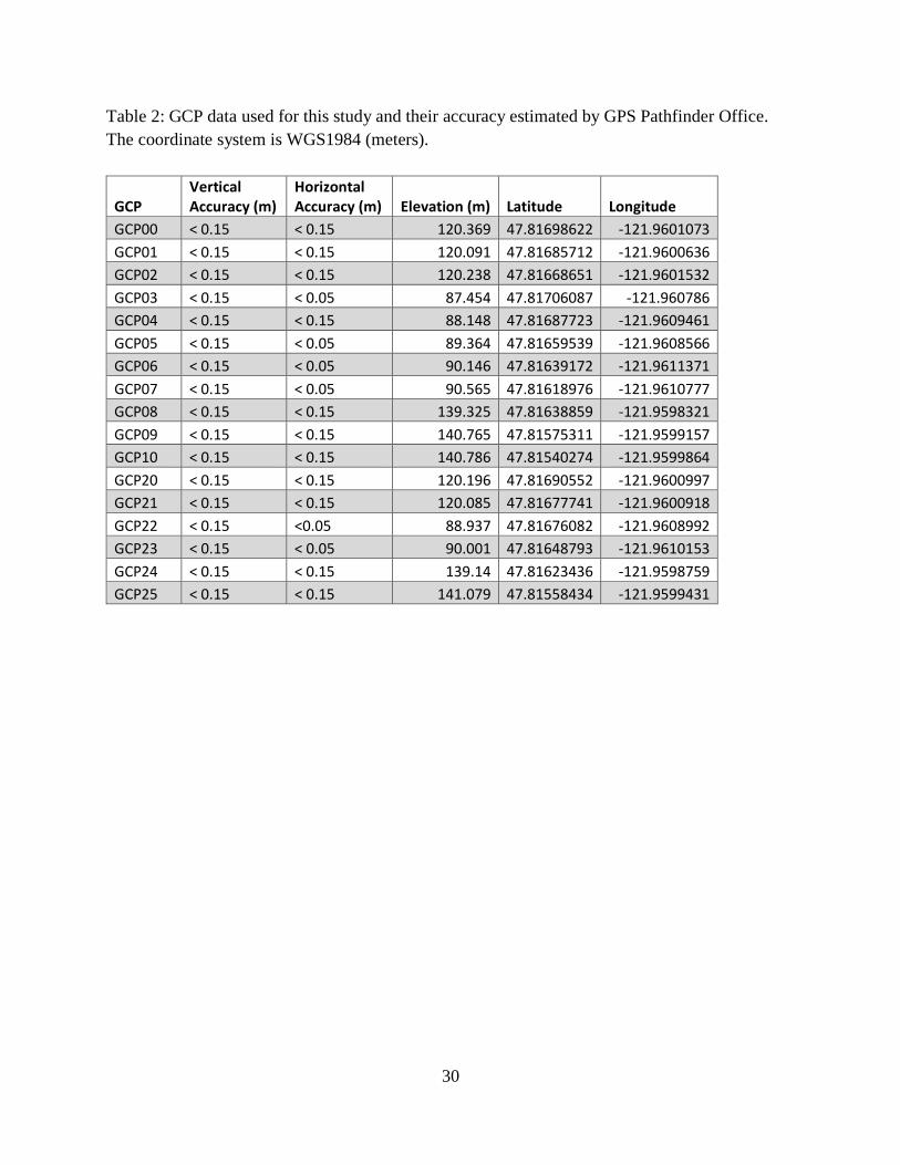
30

Table 2: GCP data used for this study and their accuracy estimated by GPS Pathfinder Office.

The coordinate system is WGS1984 (meters).

GCP Vertical Accuracy (m)

Horizontal Accuracy (m) Elevation (m) Latitude Longitude

GCP00 < 0.15 < 0.15 120.369 47.81698622 -121.9601073

GCP01 < 0.15 < 0.15 120.091 47.81685712 -121.9600636

GCP02 < 0.15 < 0.15 120.238 47.81668651 -121.9601532

GCP03 < 0.15 < 0.05 87.454 47.81706087 -121.960786

GCP04 < 0.15 < 0.15 88.148 47.81687723 -121.9609461

GCP05 < 0.15 < 0.05 89.364 47.81659539 -121.9608566

GCP06 < 0.15 < 0.05 90.146 47.81639172 -121.9611371

GCP07 < 0.15 < 0.05 90.565 47.81618976 -121.9610777

GCP08 < 0.15 < 0.15 139.325 47.81638859 -121.9598321

GCP09 < 0.15 < 0.15 140.765 47.81575311 -121.9599157

GCP10 < 0.15 < 0.15 140.786 47.81540274 -121.9599864

GCP20 < 0.15 < 0.15 120.196 47.81690552 -121.9600997

GCP21 < 0.15 < 0.15 120.085 47.81677741 -121.9600918

GCP22 < 0.15 <0.05 88.937 47.81676082 -121.9608992

GCP23 < 0.15 < 0.05 90.001 47.81648793 -121.9610153

GCP24 < 0.15 < 0.15 139.14 47.81623436 -121.9598759

GCP25 < 0.15 < 0.15 141.079 47.81558434 -121.9599431

31

Table 3: RMSE calculations using the GCPs and SfM model.

GCP GCP H Accuracy (m)

GCP V Accuracy (m)

(SfM-GCP) H Error (m)

GCP Elev (m)

SfM Elev (m)

20 < 0.015 < 0.015 0.025 120.196 120.127

21 < 0.015 < 0.015 0.053 120.085 119.941

22 < 0.05 < 0.015 0.067 88.937 89.031

23 < 0.05 < 0.015 0.04 90.001 90.001

24 < 0.15 < 0.015 0.08 139.14 139.296

25 < 0.15 < 0.015 0.194 141.079 140.852

(SfM-GCP) V Error (m)

(SfM-GCP) Error (m)

(SfM-GCP) Error^2

-0.069 0.0734 0.0054

-0.144 0.1534 0.0235

0.094 0.1154 0.0133

0 0.0400 0.0016

0.156 0.1753 0.0307

-0.227 0.2986 0.0892

Average Error^2 0.0273

RMSE (m) 0.17

A

Appendix A

Cadman Quarry SfM Hillshade

This is a hillshade of the rockslide at Cadman Quarry derived using SfM. Resolution: 4.0cm.

B

Appendix B

The purpose of the Master’s in Earth and Space Sciences – Applied Geosciences (MESSAGe)

internship project is to give students the ability to familiarize themselves with planning,

implementing, and completing a research project with professionals in the geosciences industry.

The MESSAGe internship project requires the students to each write a technical report covering

their project as well as perform an oral presentation. Each student works under the guidance of a

mentor who is skilled in the area of the student’s research. Each student will also work with a

group of two to three professional geoscientists, one of whom is the student’s mentor, to review

and edit the student’s project proposal and technical report.