9CALCULATING CONSUMER PRICEINDICES IN PRACTICE

Introduction9.1 The purpose of this chapter is to provide a general

description of the ways in which consumer price indices(CPIs) are calculated in practice. The methods used indifferent countries are not exactly the same, but they havemuch in common. There is clearly interest from bothcompilers and users of CPIs in knowing how most sta-tistical offices actually set about calculating their CPIs.9.2 As a result of the greater insights into the prop-

erties and behaviour of price indices that have beenachieved in recent years, it is now recognized that sometraditional methods may not necessarily be optimal froma conceptual and theoretical viewpoint. Concerns havealso been voiced in a number of countries about possiblebiases that may be affecting CPIs. These issues andconcerns need to be considered in this manual. Of course,the methods used to compile CPIs are inevitably con-strained by the resources available, not merely for col-lecting and processing prices, but also for gathering theexpenditure data needed for weighting purposes. In somecountries, the methods used may be severely constrainedby lack of resources.9.3 The calculation of CPIs usually proceeds in two

stages. First, price indices are estimated for the elemen-tary expenditure aggregates, or simply elementary aggre-gates. Then these elementary price indices are averagedto obtain higher-level indices using the relative values ofthe elementary expenditure aggregates as weights. Thischapter starts by explaining how the elementary aggre-gates are constructed, and what economic and statisticalcriteria need to be taken into consideration in definingthe aggregates. The index number formulae most com-monly used to calculate the elementary indices are thenpresented, and their properties and behaviour illustratedusing numerical examples. The pros and cons of thevarious formulae are considered, together with somealternative formulae that might be used instead. Theproblems created by disappearing and new items are alsoexplained, as well as the different ways of imputingvalues for missing prices.9.4 The second part of the chapter is concerned with

the calculation of higher-level indices. The focus is on theongoing production of a monthly price index in whichthe elementary price indices are averaged, or aggregated,to obtain higher-level indices. Price-updating of weights,chain linking and reweighting are discussed, with ex-amples being provided. The problems associated withintroduction of new elementary price indices and newhigher-level indices into the CPI are also dealt with. It isexplained how it is possible to decompose the change inthe overall index into its component parts. Finally, the

possibility of using some alternative and rather morecomplex index formulae is considered.

9.5 The chapter concludes with a section on dataediting procedures, as these are an integral part of theprocess of compiling CPIs. It is essential to ensure thatthe right data are entered into the various formulae.There may be errors resulting from the inclusion ofincorrect data or from entering correct data inappro-priately, and errors resulting from the exclusion of cor-rect data that are mistakenly believed to be wrong. Thesection examines data editing procedures which try tominimize both types of errors.

The calculation of price indicesfor elementary aggregates

9.6 CPIs are typically calculated in two steps. In thefirst step, the elementary price indices for the elementaryaggregates are calculated. In the second step, higher-level indices are calculated by averaging the elementaryprice indices. The elementary aggregates and their priceindices are the basic building blocks of the CPI.

Construction of elementary aggregates9.7 Elementary aggregates are groups of relatively

homogeneous goods and services. They may cover thewhole country or separate regions within the country.Likewise, elementary aggregates may be distinguishedfor different types of outlets. The nature of the elemen-tary aggregates depends on circumstances and the avail-ability of information. Elementary aggregates maytherefore be defined differently in different countries.Some key points, however, should be noted:

� Elementary aggregates should consist of groups ofgoods or services that are as similar as possible, andpreferably fairly homogeneous.

� They should also consist of items that may beexpected to have similar price movements. Theobjective should be to try to minimize the dispersionof price movements within the aggregate.

� The elementary aggregates should be appropriate toserve as strata for sampling purposes in the light ofthe sampling regime planned for the data collection.

9.8 Each elementary aggregate, whether relatingto the whole country or an individual region or groupof outlets, will typically contain a very large number ofindividual goods or services, or items. In practice, only asmall number can be selected for pricing. When selectingthe items, the following considerations need to be taken

153

into account:

� The items selected should be ones for which pricemovements are believed to be representative of all theproducts within the elementary aggregate.

� The number of items within each elementary aggregatefor which prices are collected should be large enoughfor the estimated price index to be statistically reliable.The minimum number required will vary betweenelementary aggregates depending on the nature of theproducts and their price behaviour.

� The object is to try to track the price of the same itemover time for as long as possible, or as long as the itemcontinues to be representative. The items selectedshould therefore be ones that are expected to remainon the market for some time, so that like can becompared with like.

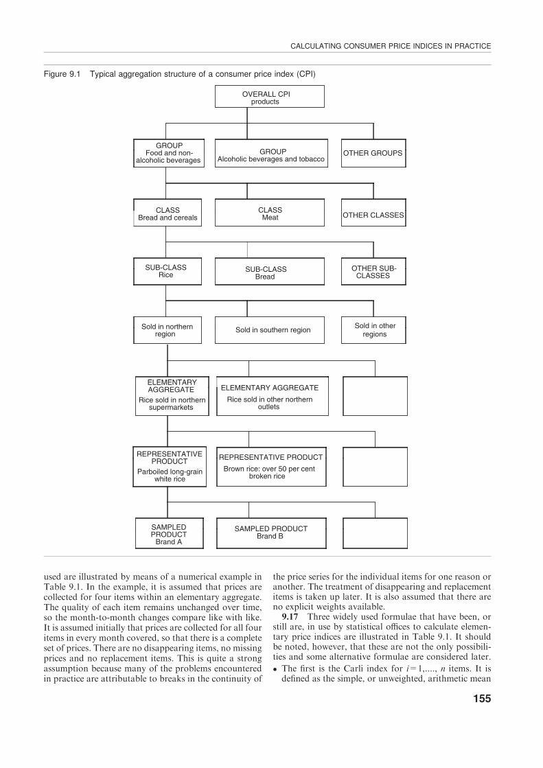
9.9 The aggregation structure. The aggregationstructure for a CPI is illustrated in Figure 9.1. Using aclassification of consumers’ expenditures such as theClassification of Individual Consumption according toPurpose (COICOP), the entire set of consumption goodsand services covered by the overall CPI can be dividedinto groups, such as ‘‘food and non-alcoholic beverages’’.Each group is further divided into classes, such as ‘‘food’’.For CPI purposes, each class can then be further dividedinto more homogeneous sub-classes, such as ‘‘rice’’. Thesub-classes are the equivalent of the basic headings used inthe International Comparison Program (ICP), whichcalculates purchasing power parities (PPPs) betweencountries. Finally, the sub-class may be further sub-divided to obtain the elementary aggregates, by dividingaccording to region or type of outlet, as in Figure 9.1. Insome cases, a particular sub-class cannot be, or does notneed to be, further subdivided, in which case the sub-classbecomes the elementary aggregate. Within each elemen-tary aggregate, one or more items are selected to representall the items in the elementary aggregate. For example, theelementary aggregate consisting of rice sold in super-markets in the northern region covers all types of rice,from which parboiled white rice and brown rice with over50 per cent broken grains are selected as representativeitems. Of course, more representative items might beselected in practice. Finally, for each representative item,a number of specific products can be selected for pricecollection, such as particular brands of parboiled rice.Again, the number of sampled products selectedmay varydepending on the nature of the representative product.

9.10 Methods used to calculate the elementary indi-ces from the individual price observations are discussedbelow. Working upwards from the elementary priceindices, all indices above the elementary aggregate levelare higher-level indices that can be calculated from theelementary price indices using the elementary expendi-ture aggregates as weights. The aggregation structure isconsistent, so that the weight at each level above theelementary aggregate is always equal to the sum of itscomponents. The price index at each higher level ofaggregation can be calculated on the basis of the weightsand price indices for its components, that is, the lower-level or elementary indices. The individual elementaryprice indices are not necessarily sufficiently reliable to be

published separately, but they remain the basic buildingblocks of all higher-level indices.

9.11 Weights within elementary aggregates. In mostcases, the price indices for elementary aggregates arecalculatedwithout the use of explicit expenditure weights.Whenever possible, however, weights should be used thatreflect the relative importance of the sampled items, evenif the weights are only approximate. Often, the elemen-tary aggregate is simply the lowest level at which reliableweighting information is available. In this case, the ele-mentary index has to be calculated as an unweightedaverage of the prices of which it consists. Even in thiscase, however, it should be noted that when the items areselected with probabilities proportional to the size ofsome relevant variable such as sales, weights are impli-citly introduced by the sampling selection procedure.

9.12 For certain elementary aggregates, informationabout sales of particular items, market shares and re-gional weights may be used as explicit weights within anelementary aggregate. Weights within elementary aggre-gates may be updated independently and possibly moreoften than the elementary aggregates themselves (whichserve as weights for the higher-level indices).

9.13 For example, assume that the number of sup-pliers of a certain product such as fuel for cars is limited.The market shares of the suppliers may be known frombusiness survey statistics and can be used as weights inthe calculation of an elementary aggregate price indexfor car fuel. Alternatively, prices for water may be col-lected from a number of local water supply serviceswhere the population in each local region is known. Therelative size of the population in each region may then beused as a proxy for the relative consumption expendi-tures to weight the price in each region to obtain theelementary aggregate price index for water.

9.14 A special situation occurs in the case of tariffprices. A tariff is a list of prices for the purchase of aparticular kind of good or service under different termsand conditions. One example is electricity, where one priceis charged during daytime while a lower price is charged atnight. Similarly, a telephone company may charge a lowerprice for a call at the weekend than in the rest of the week.Another example may be bus tickets sold at one price toordinary passengers and at lower prices to children or oldage pensioners. In such cases, it is appropriate to assignweights to the different tariffs or prices in order to calcu-late the price index for the elementary aggregate.

9.15 The increasing use of electronic points of sale inmany countries, in which both prices and quantities arescanned as the purchases are made, means that valuablenew sources of information may become increasinglyavailable to statistical offices. This could lead to sig-nificant changes in the ways in which price data arecollected and processed for CPI purposes. The treatmentof scanner data is examined in Chapters 7, 8 and 21.

Construction of elementary price indices9.16 An elementary price index is the price index for

an elementary aggregate. Various different methods andformulae may be used to calculate elementary priceindices. The methods that have been most commonly

CONSUMER PRICE INDEX MANUAL: THEORY AND PRACTICE

154

used are illustrated by means of a numerical example inTable 9.1. In the example, it is assumed that prices arecollected for four items within an elementary aggregate.The quality of each item remains unchanged over time,so the month-to-month changes compare like with like.It is assumed initially that prices are collected for all fouritems in every month covered, so that there is a completeset of prices. There are no disappearing items, no missingprices and no replacement items. This is quite a strongassumption because many of the problems encounteredin practice are attributable to breaks in the continuity of

the price series for the individual items for one reason oranother. The treatment of disappearing and replacementitems is taken up later. It is also assumed that there areno explicit weights available.

9.17 Three widely used formulae that have been, orstill are, in use by statistical offices to calculate elemen-tary price indices are illustrated in Table 9.1. It shouldbe noted, however, that these are not the only possibili-ties and some alternative formulae are considered later.

� The first is the Carli index for i=1,...., n items. It isdefined as the simple, or unweighted, arithmetic mean

OVERALL CPIproducts

GROUPFood and non-

alcoholic beverages GROUP

Alcoholic beverages and tobacco OTHER GROUPS

CLASSBread and cereals

CLASSMeat OTHER CLASSES

SUB-CLASSRice

SUB-CLASSBread

OTHER SUB-CLASSES

Sold in northernregion Sold in southern region Sold in other

regions

ELEMENTARYAGGREGATE

Rice sold in northernsupermarkets

ELEMENTARY AGGREGATE

Rice sold in other northernoutlets

REPRESENTATIVEPRODUCT

Parboiled long-grainwhite rice

REPRESENTATIVE PRODUCT

Brown rice: over 50 per centbroken rice

SAMPLED PRODUCT

Brand A

SAMPLED PRODUCTBrand B

Figure 9.1 Typical aggregation structure of a consumer price index (CPI)

CALCULATING CONSUMER PRICE INDICES IN PRACTICE

155

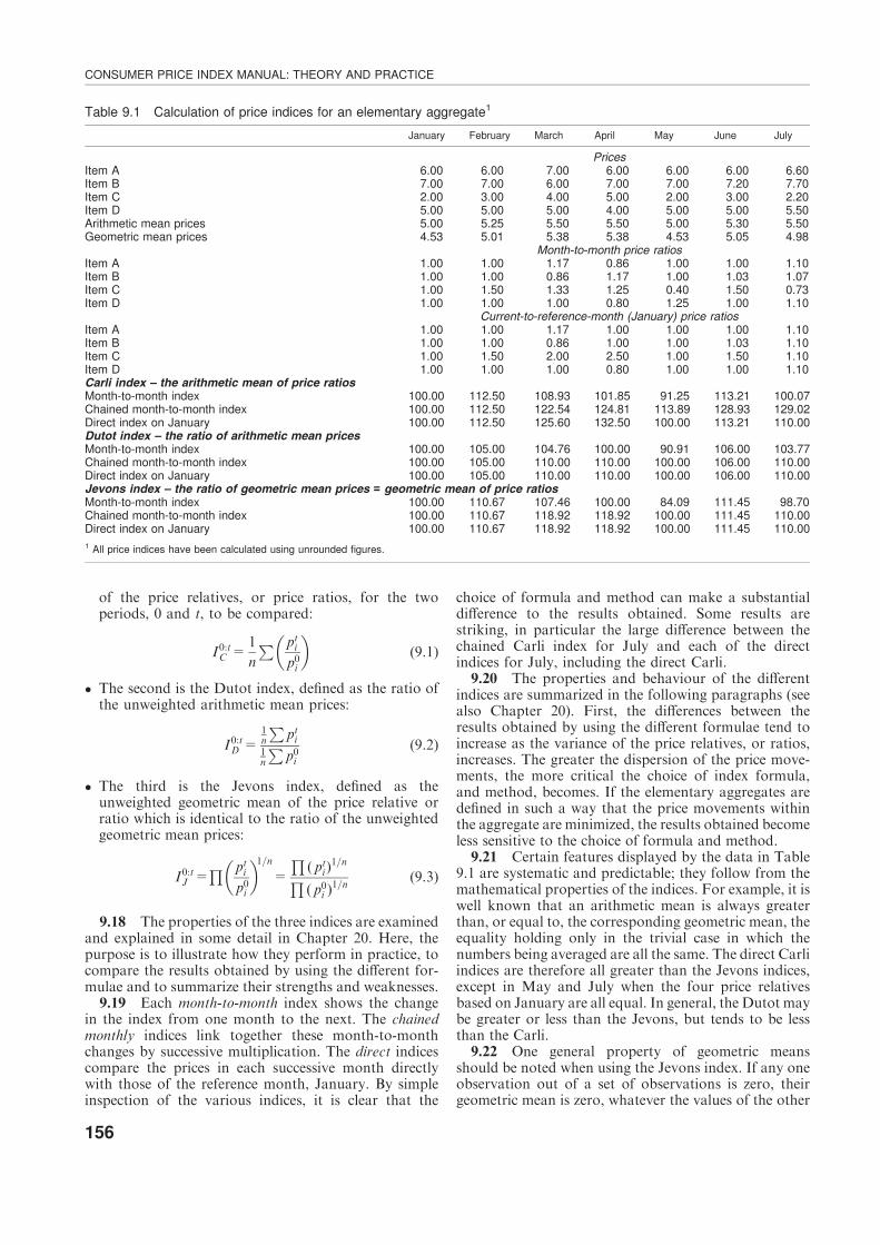
of the price relatives, or price ratios, for the twoperiods, 0 and t, to be compared:

I0:tC =

1

n

P ptip0i

� �(9.1)

� The second is the Dutot index, defined as the ratio ofthe unweighted arithmetic mean prices:

I0:tD =

1n

Ppti

1n

Pp0i

(9.2)

� The third is the Jevons index, defined as theunweighted geometric mean of the price relative orratio which is identical to the ratio of the unweightedgeometric mean prices:

I0:tJ =

Q ptip0i

� �1=n=

Q( pti)

1=nQ( p0i )

1=n(9.3)

9.18 The properties of the three indices are examinedand explained in some detail in Chapter 20. Here, thepurpose is to illustrate how they perform in practice, tocompare the results obtained by using the different for-mulae and to summarize their strengths and weaknesses.

9.19 Each month-to-month index shows the changein the index from one month to the next. The chainedmonthly indices link together these month-to-monthchanges by successive multiplication. The direct indicescompare the prices in each successive month directlywith those of the reference month, January. By simpleinspection of the various indices, it is clear that the

choice of formula and method can make a substantialdifference to the results obtained. Some results arestriking, in particular the large difference between thechained Carli index for July and each of the directindices for July, including the direct Carli.

9.20 The properties and behaviour of the differentindices are summarized in the following paragraphs (seealso Chapter 20). First, the differences between theresults obtained by using the different formulae tend toincrease as the variance of the price relatives, or ratios,increases. The greater the dispersion of the price move-ments, the more critical the choice of index formula,and method, becomes. If the elementary aggregates aredefined in such a way that the price movements withinthe aggregate are minimized, the results obtained becomeless sensitive to the choice of formula and method.

9.21 Certain features displayed by the data in Table9.1 are systematic and predictable; they follow from themathematical properties of the indices. For example, it iswell known that an arithmetic mean is always greaterthan, or equal to, the corresponding geometric mean, theequality holding only in the trivial case in which thenumbers being averaged are all the same. The direct Carliindices are therefore all greater than the Jevons indices,except in May and July when the four price relativesbased on January are all equal. In general, the Dutot maybe greater or less than the Jevons, but tends to be lessthan the Carli.

9.22 One general property of geometric meansshould be noted when using the Jevons index. If any oneobservation out of a set of observations is zero, theirgeometric mean is zero, whatever the values of the other

Table 9.1 Calculation of price indices for an elementary aggregate1

January February March April May June July

PricesItem A 6.00 6.00 7.00 6.00 6.00 6.00 6.60Item B 7.00 7.00 6.00 7.00 7.00 7.20 7.70Item C 2.00 3.00 4.00 5.00 2.00 3.00 2.20Item D 5.00 5.00 5.00 4.00 5.00 5.00 5.50Arithmetic mean prices 5.00 5.25 5.50 5.50 5.00 5.30 5.50Geometric mean prices 4.53 5.01 5.38 5.38 4.53 5.05 4.98

Month-to-month price ratiosItem A 1.00 1.00 1.17 0.86 1.00 1.00 1.10Item B 1.00 1.00 0.86 1.17 1.00 1.03 1.07Item C 1.00 1.50 1.33 1.25 0.40 1.50 0.73Item D 1.00 1.00 1.00 0.80 1.25 1.00 1.10

Current-to-reference-month (January) price ratiosItem A 1.00 1.00 1.17 1.00 1.00 1.00 1.10Item B 1.00 1.00 0.86 1.00 1.00 1.03 1.10Item C 1.00 1.50 2.00 2.50 1.00 1.50 1.10Item D 1.00 1.00 1.00 0.80 1.00 1.00 1.10Carli index – the arithmetic mean of price ratiosMonth-to-month index 100.00 112.50 108.93 101.85 91.25 113.21 100.07Chained month-to-month index 100.00 112.50 122.54 124.81 113.89 128.93 129.02Direct index on January 100.00 112.50 125.60 132.50 100.00 113.21 110.00Dutot index – the ratio of arithmetic mean pricesMonth-to-month index 100.00 105.00 104.76 100.00 90.91 106.00 103.77Chained month-to-month index 100.00 105.00 110.00 110.00 100.00 106.00 110.00Direct index on January 100.00 105.00 110.00 110.00 100.00 106.00 110.00Jevons index – the ratio of geometric mean prices = geometric mean of price ratiosMonth-to-month index 100.00 110.67 107.46 100.00 84.09 111.45 98.70Chained month-to-month index 100.00 110.67 118.92 118.92 100.00 111.45 110.00Direct index on January 100.00 110.67 118.92 118.92 100.00 111.45 110.00

1 All price indices have been calculated using unrounded figures.

CONSUMER PRICE INDEX MANUAL: THEORY AND PRACTICE

156

observations. The Jevons index is sensitive to extremefalls in prices and it may be necessary to impose upperand lower bounds on the individual price ratios of say 10and 0.1, respectively, when using the Jevons. Of course,extreme observations often result from errors of one kindor another, so extreme price movements should becarefully checked anyway.9.23 Another important property of the indices

illustrated in Table 9.1 is that the Dutot and the Jevonsindices are transitive, whereas the Carli is not. Transi-tivity means that the chained monthly indices are iden-tical to the corresponding direct indices. This property isimportant in practice, because many elementary priceindices are in fact calculated as chain indices which linktogether the month-on-month indices. The intransitivityof the Carli index is illustrated dramatically in Table 9.1when each of the four individual prices in May returnsto the same level as it was in January, but the chain Carliregisters an increase of almost 14 per cent over January.Similarly, in July, although each individual price isexactly 10 per cent higher than in January, the chainCarli registers an increase of 29 per cent. These resultswould be regarded as perverse and unacceptable in thecase of a direct index, but even in the case of a chainindex the results seems so intuitively unreasonable as toundermine the credibility of the chain Carli. The pricechanges between March and April illustrate the effectsof ‘‘price bouncing’’ in which the same four prices areobserved in both periods but they are switched betweenthe different items. The monthly Carli index fromMarchto April increases whereas both the Dutot and theJevons indices are unchanged.9.24 The message emerging from this brief illustra-

tion of the behaviour of just three possible formulae isthat different index numbers and methods can deliververy different results. Index compilers have to familiarizethemselves with the interrelationships between the vari-ous formulae at their disposal for the calculation ofthe elementary price indices so that they are aware ofthe implications of choosing one formula rather thananother. Knowledge of these interrelationships is never-theless not sufficient to determine which formula shouldbe used, even though it makes it possible to make a moreinformed and reasoned choice. It is necessary to appealto other criteria in order to settle the choice of formula.There are two main approaches that may be used, theaxiomatic and the economic approaches.

Axiomatic approach to elementaryprice indices9.25 As explained in Chapters 16 and 20, one way in

which to decide upon an appropriate index formula is torequire it to satisfy certain specified axioms or tests. Thetests throw light on the properties possessed by differentkinds of indices, some of which may not be intuitivelyobvious. Four basic tests will be cited here to illustratethe axiomatic approach:

� Proportionality test – if all prices are l times the pricesin the price reference period (January in the example),the index should equal l. The data for July, whenevery price is 10 per cent higher than in January, show

that all three direct indices satisfy this test. A specialcase of this test is the identity test, which requires thatif the price of every item is the same as in the referenceperiod, the index should be equal to unity (as in Mayin the example).

� Changes in the units of measurement test (commen-surability test) – the price index should not change ifthe quantity units in which the products are measuredare changed (for example, if the prices are expressedper litre rather than per pint). The Dutot index failsthis test, as explained below, but the Carli and Jevonsindices satisfy the test.

� Time reversal test – if all the data for the two periodsare interchanged, then the resulting price index shouldequal the reciprocal of the original price index. TheCarli index fails this test, but the Dutot and the Jevonsindices both satisfy the test. The failure of the Carli tosatisfy the test is not immediately obvious from theexample, but can easily be verified by interchangingthe prices in January and April, for example, in whichcase the backwards Carli for January based on Aprilis equal to 91.3 whereas the reciprocal of the forwardsCarli is 1/132.5 or 75.5.

� Transitivity test – the chain index between two periodsshould equal the direct index between the same twoperiods. It can be seen from the example that theJevons and the Dutot indices both satisfy this test,whereas the Carli index does not. For example,although the prices in May have returned to the samelevels as in January, the chain Carli registers 113.9.This illustrates the fact that the Carli may have a sig-nificant built-in upward bias.

9.26 Many other axioms or tests can be devised, butthe above are sufficient to illustrate the approach andalso to throw light on some important features of theelementary indices under consideration here.

9.27 The sets of products covered by elementaryaggregates are meant to be as homogeneous as possible.If they are not fairly homogeneous, the failure of theDutot index to satisfy the units of measurement orcommensurablity test can be a serious disadvantage.Although defined as the ratio of the unweighted arith-metic average prices, the Dutot index may also beinterpreted as a weighted arithmetic average of the priceratios in which each ratio is weighted by its price in thebase period. This can be seen by rewriting formula (9.2)above as

I0:tD =

1n

Pp0i ( p

ti=p

0i )

1n

Pp0i

However, if the products are not homogeneous, therelative prices of the different items may depend quitearbitrarily on the quantity units in which they are mea-sured.

9.28 Consider, for example, salt and pepper, whichare found within the same sub-class of COICOP. Sup-pose the unit of measurement for pepper is changedfrom grams to ounces, while leaving the units in whichsalt is measured (say kilos) unchanged. As an ounce ofpepper is equal to 28.35 grams, the ‘‘price’’ of pepper

CALCULATING CONSUMER PRICE INDICES IN PRACTICE

157

increases by over 28 times, which effectively increasesthe weight given to pepper in the Dutot index by over 28times. The price of pepper relative to salt is inherentlyarbitrary, depending entirely on the choice of units inwhich to measure the two goods. In general, when thereare different kinds of products within the elementaryaggregate, the Dutot index is unacceptable conceptually.

9.29 The Dutot index is acceptable only when the setof items covered is homogeneous, or at least nearlyhomogeneous. For example, it may be acceptable for aset of apple prices even though the apples may be ofdifferent varieties, but not for the prices of a number ofdifferent kinds of fruits, such as apples, pineapples andbananas, some of which may be much more expen-sive per item or per kilo than others. Even when theitems are fairly homogeneous and measured in the sameunits, the Dutot’s implicit weights may still not besatisfactory. More weight is given to the price changesfor the more expensive items, but in practice they maywell account for only small shares of the total expendi-ture within the aggregate. Consumers are unlikely tobuy items at high prices if the same items are available atlower prices.

9.30 It may be concluded that from an axiomaicviewpoint, both the Carli and the Dutot indices, althoughthey have been, and still are, widely used by statisticaloffices, have serious disadvantages. The Carli indexfails the time reversal and transitivity tests. In principle,it should not matter whether we choose to measure pricechanges forwards or backwards in time. We wouldexpect the same answer, but this is not the case for theCarli. Chained Carli indices may be subject to a sig-nificant upward bias. The Dutot index is meaningful fora set of homogeneous items but becomes increasinglyarbitrary as the set of products becomes more diverse.On the other hand, the Jevons index satisfies all the testslisted above and also emerges as the preferred indexwhen the set of tests is enlarged, as shown in Chapter 20.From an axiomatic point of view, the Jevons index isclearly the index with the best properties, even though itmay not have been used much until recently. Thereseems to be an increasing tendency for statistical officesto switch from using Carli or Dutot indices to the Jevonsindex.

Economic approach to elementaryprice indices

9.31 In the economic approach, the objective is toestimate an economic index – that is, a cost of living indexfor the elementary aggregate (see Chapter 20). The itemsfor which prices are collected are treated as if they con-stituted a basket of goods and services purchased byconsumers, from which the consumers derive utility. Acost of living index measures the minimum amount bywhich consumers would have to change their expendi-tures in order to keep their utility level unchanged,allowing consumers to make substitutions between theitems in response to changes in the relative prices ofitems. In the absence of information about quantities orexpenditures within an elementary aggregate, the indexcan only be estimated when certain special conditions areassumed to prevail.

9.32 There are two special cases of some interest. Thefirst case is when consumers continue to consumethe same relative quantities whatever the relativeprices. Consumers prefer not to make any substitutionsin reponse to changes in relative prices. The cross-elasticities of demand are zero. The underlying pre-ferences are described in the economics literature as‘‘Leontief ’’. With these preferences, a Laspeyres indexwould provide an exact measure of the cost of livingindex. In this first case, the Carli index calculated for arandom sample would provide an estimate of the cost ofliving index provided that the items are selected withprobabilities proportional to the population expenditureshares. It might appear that if the items were selectedwith probabilities proportional to the population quan-tity shares, the sample Dutot would provide an estimateof the population Laspeyres. If the basket for the Las-peyres index contains different kinds of products whosequantities are not additive, however, the quantity shares,and hence the probabilities, are undefined.

9.33 The second case occurs when consumers areassumed to vary the quantities they consume in inverseproportion to the changes in relative prices. The cross-elasticities of demand between the different items are allunity, the expenditure shares being the same in bothperiods. The underlying preferences are described as‘‘Cobb–Douglas’’. With these preferences, the geometricLaspeyres would provide an exact measure of the cost ofliving index. The geometric Laspeyres is a weightedgeometric average of the price relatives, using the expen-diture shares in the earlier period as weights (the expen-diture shares in the second period would be the same inthe particular case under consideration). In this secondcase, the Jevons index calculated for a random samplewould provide an unbiased estimate of the cost of livingindex, provided that the items are selected with prob-abilities proportional to the population expenditureshares.

9.34 On the basis of the economic approach, thechoice between the sample Jevons and the sample Carlirests on which is likely to approximate the more closelyto the underlying cost of living index: in other words, onwhether the (unknown) cross-elasticities are likely to becloser to unity or zero, on average. In practice, the cross-elasticities could take on any value ranging up to plusinfinity for an elementary aggregate consisting of a set ofstrictly homogeneous items, i.e., perfect substitutes. Itshould be noted that in the limit when the productsreally are homogeneous, there is no index number prob-lem, and the price ‘‘index’’ is given by the ratio of theunit values in the two periods, as explained later. It maybe conjectured that the average cross-elasticity is likelyto be closer to unity than zero for most elementaryaggregates so that, in general, the Jevons index is likelyto provide a closer approximation to the cost of livingindex than the Carli. In this case, the Carli index must beviewed as having an upward bias.

9.35 The insight provided by the economic approachis that the Jevons index is likely to provide a closerapproximation to the cost of living index for the ele-mentary aggregate than the Carli because, in mostcases, a significant amount of substitution is more likely

CONSUMER PRICE INDEX MANUAL: THEORY AND PRACTICE

158

than no substitution, especially as elementary aggregatesshould be deliberately constructed in such a way as togroup together similar items that are close substitutes foreach other.9.36 The Jevons index does not imply, or assume,

that expenditure shares remain constant. Obviously, theJevons can be calculated whatever changes do, or do notoccur in the expenditure shares in practice. What theeconomic approach shows is that if the expenditureshares remain constant (or roughly constant), then theJevons index can be expected to provide a good estimateof the underlying cost of living index. Similarly, if therelative quantities remain constant, then the Carli indexcan be expected to provide a good estimate, but the Carlidoes not actually imply that quantities remain fixed.9.37 It may be concluded that, on the basis of the

economic approach as well as the axiomatic approach,the Jevons emerges as the preferred index in general,although there may be cases in which little or no sub-stitution takes place within the elementary aggregateand the Carli might be preferred. The index compilermust make a judgement on the basis of the nature of theproducts actually included in the elementary aggregate.9.38 Before leaving this topic, it should be noted

that it has thrown light on some of the sampling prop-erties of the elementary indices. If the products in thesample are selected with probabilities proportional toexpenditures in the price reference period:

– the sample (unweighted) Carli index provides anunbiased estimate of the population Laspeyres;

– the sample (unweighted) Jevons index providesan unbiased estimate of the population geometricLaspeyres.

These results hold irrespective of the underlying cost ofliving index.

Chain versus direct indices forelementary aggregates9.39 In a direct elementary index, the prices of the

current period are compared directly with those of theprice reference period. In a chain index, prices in eachperiod are compared with those in the previous period,the resulting short-term indices being chained together toobtain the long-term index, as illustrated in Table 9.1.9.40 Provided that prices are recorded for the same

set of items in every period, as in Table 9.1, any indexformula defined as the ratio of the average prices will betransitive: that is, the same result is obtained whether theindex is calculated as a direct index or as a chain index. Ina chain index, successive numerators and denominatorswill cancel out, leaving only the average price in the lastperiod divided by the average price in the referenceperiod, which is the same as the direct index. Both theDutot and the Jevons indices are therefore transitive. Asalready noted, however, a chain Carli index is not tran-sitive and should not be used because of its upward bias.Nevertheless, the direct Carli remains an option.9.41 Although the chain and direct versions of the

Dutot and Jevons indices are identical when there are nobreaks in the series for the individual items, they offerdifferent ways of dealing with new and disappearing

items, missing prices and quality adjustments. In prac-tice, products continually have to be dropped from theindex and new ones included, in which case the direct andthe chain indices may differ if the imputations for missingprices are made differently.

9.42 When a replacement item has to be included in adirect index, it will often be necessary to estimate theprice of the new item in the price reference period, whichmay be some time in the past. The same happens if, as aresult of an update of the sample, new items have to belinked into the index. Assuming that no informationexists on the price of the replacement item in the pricereference period, it will be necessary to estimate it usingprice ratios calculated for the items that remain in theelementary aggregate, a subset of these items or someother indicator. However, the direct approach shouldonly be used for a limited period of time. Otherwise, mostof the reference prices would end up being imputed,which would be an undesirable outcome. This effectivelyrules out the use of the Carli index over a long period oftime, as the Carli can only be used in its direct formanyway, being unacceptable when chained. This impliesthat, in practice, the direct Carli may be used only if theoverall index is chain linked annually, or at intervals oftwo or three years.

9.43 In a chain index, if an item becomes perma-nently missing, a replacement item can be linked into theindex as part of the ongoing index calculation byincluding the item in the monthly index as soon as pricesfor two successive months are obtained. Similarly, if thesample is updated and new products have to be linkedinto the index, this will require successive old and newprices for the present and the preceding months. For achain index, however, the missing observation will havean impact on the index for two months, since the missingobservation is part of two links in the chain. This is notthe case for a direct index, where a single, non-estimatedmissing observation will only have an impact on theindex in the current period. For example, for a com-parison between periods 0 and 3, a missing price of anitem in period 2 means that the chain index excludes theitem for the last link of the index in periods 2 and 3, whilethe direct index includes it in period 3 since a direct indexwill be based on items whose prices are available inperiods 0 and 3. In general, however, the use of a chainindex can make the estimation of missing prices and theintroduction of replacements easier from a computa-tional point of view, whereas it may be inferred that adirect index will limit the usefulness of overlap methodsfor dealing with missing observations.

9.44 The direct and the chain approaches also pro-duce different by-products that may be used for moni-toring price data. For each elementary aggregate, achain index approach gives the latest monthly pricechange, which can be useful for both data editing andimputation of missing prices. By the same token, how-ever, a direct index derives average price levels for eachelementary aggregate in each period, and this informa-tion may be a useful by-product. Nevertheless, becausethe availability of cheap computing power and of spread-sheets allows such by-products to be calculated whethera direct or a chained approach is applied, the choice of

CALCULATING CONSUMER PRICE INDICES IN PRACTICE

159

formula should not be dictated by considerationsregarding by-products.

Consistency in aggregation9.45 Consistency in aggregation means that if an

index is calculated stepwise by aggregating lower-levelindices to obtain indices at progressively higher levels ofaggregation, the same overall result should be obtainedas if the calculation had been made in one step. Forpresentational purposes this is an advantage. If the ele-mentary aggregates are calculated using one formula andthe elementary aggregates are averaged to obtain thehigher-level indices using another formula, the resultingCPI is not consistent in aggregation. It may be argued,however, that consistency in aggregation is not necessar-ily an important or even appropriate criterion, or that itis unachievable when the amount of information avail-able on quantities and expenditures is not the same atthe different levels of aggregation. In addition, theremay be different degrees of substitution within elemen-tary aggregates as compared to the degree of substitutionbetween products in different elementary aggregates.

9.46 As noted earlier, the Carli index would beconsistent in aggregation with the Laspeyres index if theitems were to be selected with probabilities proportionalto expenditures in the reference period. This is typicallynot the case. The Dutot and the Jevons indices are alsonot consistent in aggregation with a higher-level Las-peyres. As explained below, however, the CPIs actuallycalculated by statistical offices are usually not true Las-peyres indices anyway, even though they may be basedon fixed baskets of goods and services. As also notedearlier, if the higher-level index were to be defined as ageometric Laspeyres, consistency in aggregation could beachieved by using the Jevons index for the elementaryindices at the lower level, provided that the individualitems are sampled with probabilities proportional toexpenditures. Although unfamiliar, a geometric Las-peyres has desirable properties from an economic pointof view and is considered again later.

Missing price observations9.47 The price of an item may fail to be collected in

some period either because the item is missing tem-porarily or because it has permanently disappeared. Thetwo classes of missing prices require different treatment.Temporary unavailability may occur for seasonal items(particularly for fruit, vegetables and clothing), becauseof supply shortages or possibly because of some collec-tion difficulty (say, an outlet was closed or a price col-lector was ill). The treatment of seasonal items raises anumber of particular problems. These are dealt with inChapter 22 and will not be discussed here.

9.48 The treatment of temporarily missing prices. Inthe case of temporarily missing observations for non-seasonal items, one of four actions may be taken:

– omit the item for which the price is missing so that amatched sample is maintained (like is compared withlike) even though the sample is depleted;

– carry forward the last observed price;

– impute the missing price by the average price changefor the prices that are available in the elementaryaggregate;

– impute the missing price by the price change for aparticular comparable item from another similaroutlet.

9.49 Omitting an observation from the calculationof an elementary index is equivalent to assuming thatthe price would have moved in the same way as theaverage of the prices of the items that remain included inthe index. Omitting an observation changes the implicitweights attached to the other prices in the elementaryaggregate.

9.50 Carrying forward the last observed price shouldbe avoided wherever possible and is acceptable only for avery limited number of periods. Special care needs to betaken in periods of high inflation or when markets arechanging rapidly as a result of a high rate of innovationand product turnover. While simple to apply, carryingforward the last observed price biases the resulting indextowards zero change. In addition, there is likely to be acompensating step-change in the index when the price ofthe missing item is recorded again, which will be wronglymissed by a chain index, but will be included in a directindex to return the index to its proper value. The adverseeffect on the index will be increasingly severe if the itemremains unpriced for some length of time. In general, tocarry forward is not an acceptable procedure or solutionto the problem.

9.51 Imputation of the missing price by the averagechange of the available prices may be applied for ele-mentary aggregates where the prices can be expected tomove in the same direction. The imputation can be madeusing all of the remaining prices in the elementaryaggregate. As already noted, this is numerically equiva-lent to omitting the item for the immediate period, but itis useful to make the imputation so that if the pricebecomes available again in a later period the sample sizeis not reduced in that period. In some cases, dependingon the homogeneity of the elementary aggregate, it maybe preferable to use only a subset of items from the ele-mentary aggregate to estimate the missing price. In someinstances, this may even be a single comparable itemfrom a similar type of outlet whose price change can beexpected to be similar to the missing one.

9.52 Table 9.2 illustrates the calculation of the priceindex for an elementary aggregate consisting of threeitems where one of the prices is missing inMarch. Section(a) of Table 9.2 shows the indices where the missing pricehas been omitted from the calculation. The direct indicesare therefore calculated on the basis of items A, B and Cfor all months except March, where they are calculatedon the basis of items B and C only. The chained indicesare calculated on the basis of all three prices from Jan-uary to February and from April to May. From Feb-ruary to March and from March to April the monthlyindices are calculated on the basis of items B and C only.

9.53 For both the Dutot and the Jevons indices, thedirect and chain indices now differ fromMarch onwards.The first link in the chain index (January to February) isthe same as the direct index, so the two indices are

CONSUMER PRICE INDEX MANUAL: THEORY AND PRACTICE

160

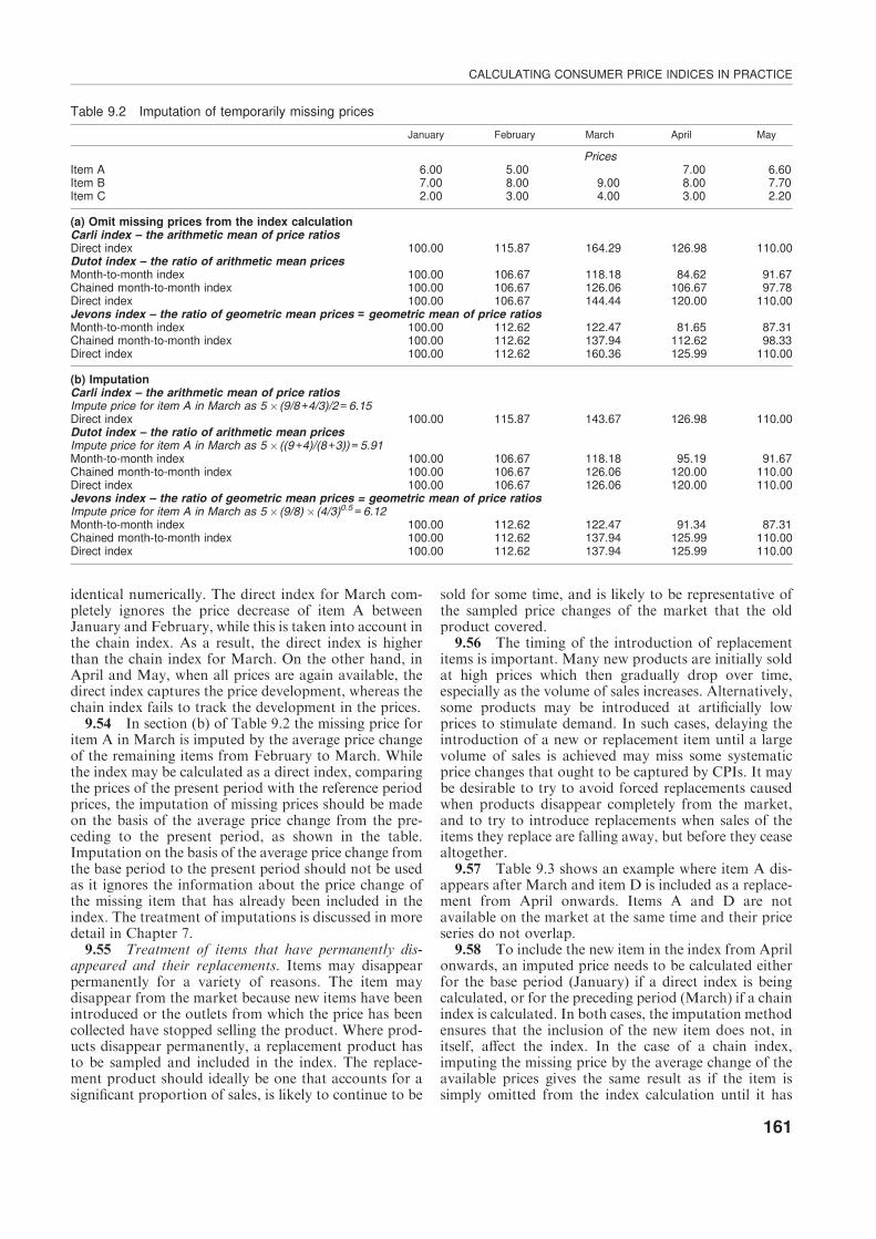
identical numerically. The direct index for March com-pletely ignores the price decrease of item A betweenJanuary and February, while this is taken into account inthe chain index. As a result, the direct index is higherthan the chain index for March. On the other hand, inApril and May, when all prices are again available, thedirect index captures the price development, whereas thechain index fails to track the development in the prices.9.54 In section (b) of Table 9.2 the missing price for

item A in March is imputed by the average price changeof the remaining items from February to March. Whilethe index may be calculated as a direct index, comparingthe prices of the present period with the reference periodprices, the imputation of missing prices should be madeon the basis of the average price change from the pre-ceding to the present period, as shown in the table.Imputation on the basis of the average price change fromthe base period to the present period should not be usedas it ignores the information about the price change ofthe missing item that has already been included in theindex. The treatment of imputations is discussed in moredetail in Chapter 7.9.55 Treatment of items that have permanently dis-

appeared and their replacements. Items may disappearpermanently for a variety of reasons. The item maydisappear from the market because new items have beenintroduced or the outlets from which the price has beencollected have stopped selling the product. Where prod-ucts disappear permanently, a replacement product hasto be sampled and included in the index. The replace-ment product should ideally be one that accounts for asignificant proportion of sales, is likely to continue to be

sold for some time, and is likely to be representative ofthe sampled price changes of the market that the oldproduct covered.

9.56 The timing of the introduction of replacementitems is important. Many new products are initially soldat high prices which then gradually drop over time,especially as the volume of sales increases. Alternatively,some products may be introduced at artificially lowprices to stimulate demand. In such cases, delaying theintroduction of a new or replacement item until a largevolume of sales is achieved may miss some systematicprice changes that ought to be captured by CPIs. It maybe desirable to try to avoid forced replacements causedwhen products disappear completely from the market,and to try to introduce replacements when sales of theitems they replace are falling away, but before they ceasealtogether.

9.57 Table 9.3 shows an example where item A dis-appears after March and item D is included as a replace-ment from April onwards. Items A and D are notavailable on the market at the same time and their priceseries do not overlap.

9.58 To include the new item in the index from Aprilonwards, an imputed price needs to be calculated eitherfor the base period (January) if a direct index is beingcalculated, or for the preceding period (March) if a chainindex is calculated. In both cases, the imputation methodensures that the inclusion of the new item does not, initself, affect the index. In the case of a chain index,imputing the missing price by the average change of theavailable prices gives the same result as if the item issimply omitted from the index calculation until it has

Table 9.2 Imputation of temporarily missing prices

January February March April May

PricesItem A 6.00 5.00 7.00 6.60Item B 7.00 8.00 9.00 8.00 7.70Item C 2.00 3.00 4.00 3.00 2.20

(a) Omit missing prices from the index calculationCarli index – the arithmetic mean of price ratiosDirect index 100.00 115.87 164.29 126.98 110.00Dutot index – the ratio of arithmetic mean pricesMonth-to-month index 100.00 106.67 118.18 84.62 91.67Chained month-to-month index 100.00 106.67 126.06 106.67 97.78Direct index 100.00 106.67 144.44 120.00 110.00Jevons index – the ratio of geometric mean prices = geometric mean of price ratiosMonth-to-month index 100.00 112.62 122.47 81.65 87.31Chained month-to-month index 100.00 112.62 137.94 112.62 98.33Direct index 100.00 112.62 160.36 125.99 110.00

(b) ImputationCarli index – the arithmetic mean of price ratiosImpute price for item A in March as 5 �(9/8+4/3)/2=6.15Direct index 100.00 115.87 143.67 126.98 110.00Dutot index – the ratio of arithmetic mean pricesImpute price for item A in March as 5 �((9+4)/(8+3))=5.91Month-to-month index 100.00 106.67 118.18 95.19 91.67Chained month-to-month index 100.00 106.67 126.06 120.00 110.00Direct index 100.00 106.67 126.06 120.00 110.00Jevons index – the ratio of geometric mean prices = geometric mean of price ratiosImpute price for item A in March as 5 �(9/8) �(4/3)0.5=6.12Month-to-month index 100.00 112.62 122.47 91.34 87.31Chained month-to-month index 100.00 112.62 137.94 125.99 110.00Direct index 100.00 112.62 137.94 125.99 110.00

CALCULATING CONSUMER PRICE INDICES IN PRACTICE

161

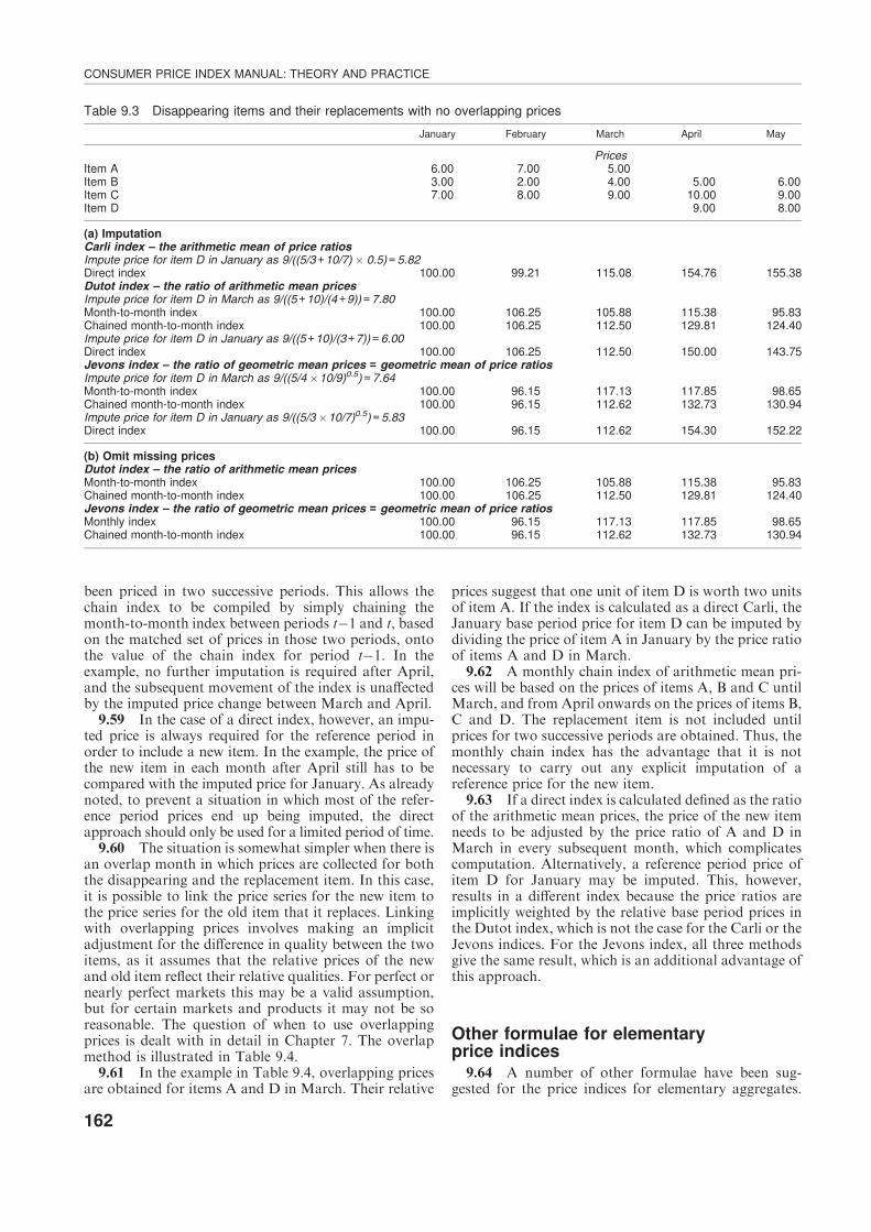
been priced in two successive periods. This allows thechain index to be compiled by simply chaining themonth-to-month index between periods t�1 and t, basedon the matched set of prices in those two periods, ontothe value of the chain index for period t�1. In theexample, no further imputation is required after April,and the subsequent movement of the index is unaffectedby the imputed price change between March and April.

9.59 In the case of a direct index, however, an impu-ted price is always required for the reference period inorder to include a new item. In the example, the price ofthe new item in each month after April still has to becompared with the imputed price for January. As alreadynoted, to prevent a situation in which most of the refer-ence period prices end up being imputed, the directapproach should only be used for a limited period of time.

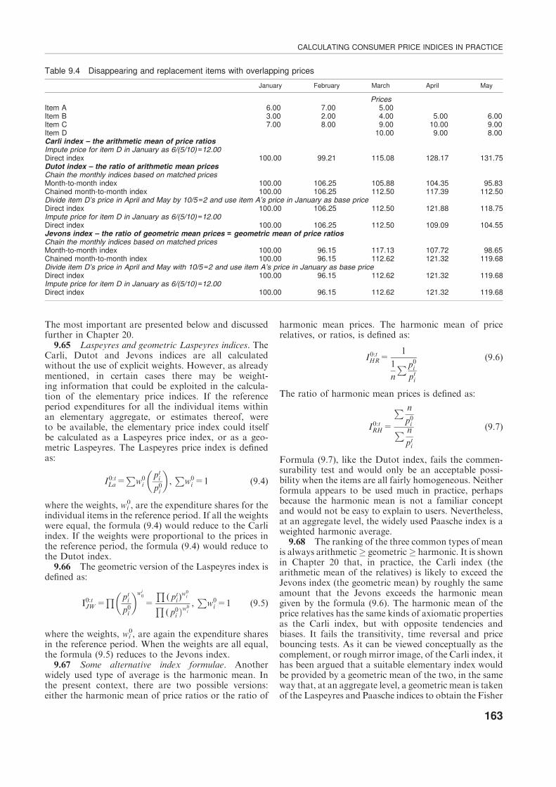
9.60 The situation is somewhat simpler when there isan overlap month in which prices are collected for boththe disappearing and the replacement item. In this case,it is possible to link the price series for the new item tothe price series for the old item that it replaces. Linkingwith overlapping prices involves making an implicitadjustment for the difference in quality between the twoitems, as it assumes that the relative prices of the newand old item reflect their relative qualities. For perfect ornearly perfect markets this may be a valid assumption,but for certain markets and products it may not be soreasonable. The question of when to use overlappingprices is dealt with in detail in Chapter 7. The overlapmethod is illustrated in Table 9.4.

9.61 In the example in Table 9.4, overlapping pricesare obtained for items A and D in March. Their relative

prices suggest that one unit of item D is worth two unitsof item A. If the index is calculated as a direct Carli, theJanuary base period price for item D can be imputed bydividing the price of item A in January by the price ratioof items A and D in March.

9.62 A monthly chain index of arithmetic mean pri-ces will be based on the prices of items A, B and C untilMarch, and from April onwards on the prices of items B,C and D. The replacement item is not included untilprices for two successive periods are obtained. Thus, themonthly chain index has the advantage that it is notnecessary to carry out any explicit imputation of areference price for the new item.

9.63 If a direct index is calculated defined as the ratioof the arithmetic mean prices, the price of the new itemneeds to be adjusted by the price ratio of A and D inMarch in every subsequent month, which complicatescomputation. Alternatively, a reference period price ofitem D for January may be imputed. This, however,results in a different index because the price ratios areimplicitly weighted by the relative base period prices inthe Dutot index, which is not the case for the Carli or theJevons indices. For the Jevons index, all three methodsgive the same result, which is an additional advantage ofthis approach.

Other formulae for elementaryprice indices

9.64 A number of other formulae have been sug-gested for the price indices for elementary aggregates.

Table 9.3 Disappearing items and their replacements with no overlapping prices

January February March April May

PricesItem A 6.00 7.00 5.00Item B 3.00 2.00 4.00 5.00 6.00Item C 7.00 8.00 9.00 10.00 9.00Item D 9.00 8.00

(a) ImputationCarli index – the arithmetic mean of price ratiosImpute price for item D in January as 9/((5/3+10/7) � 0.5)= 5.82Direct index 100.00 99.21 115.08 154.76 155.38Dutot index – the ratio of arithmetic mean pricesImpute price for item D in March as 9/((5+10)/(4+9))=7.80Month-to-month index 100.00 106.25 105.88 115.38 95.83Chained month-to-month index 100.00 106.25 112.50 129.81 124.40Impute price for item D in January as 9/((5+10)/(3+7))=6.00Direct index 100.00 106.25 112.50 150.00 143.75Jevons index – the ratio of geometric mean prices = geometric mean of price ratiosImpute price for item D in March as 9/((5/4 �10/9)0.5)=7.64Month-to-month index 100.00 96.15 117.13 117.85 98.65Chained month-to-month index 100.00 96.15 112.62 132.73 130.94Impute price for item D in January as 9/((5/3 �10/7)0.5)=5.83Direct index 100.00 96.15 112.62 154.30 152.22

(b) Omit missing pricesDutot index – the ratio of arithmetic mean pricesMonth-to-month index 100.00 106.25 105.88 115.38 95.83Chained month-to-month index 100.00 106.25 112.50 129.81 124.40Jevons index – the ratio of geometric mean prices = geometric mean of price ratiosMonthly index 100.00 96.15 117.13 117.85 98.65Chained month-to-month index 100.00 96.15 112.62 132.73 130.94

CONSUMER PRICE INDEX MANUAL: THEORY AND PRACTICE

162

The most important are presented below and discussedfurther in Chapter 20.9.65 Laspeyres and geometric Laspeyres indices. The

Carli, Dutot and Jevons indices are all calculatedwithout the use of explicit weights. However, as alreadymentioned, in certain cases there may be weight-ing information that could be exploited in the calcula-tion of the elementary price indices. If the referenceperiod expenditures for all the individual items withinan elementary aggregate, or estimates thereof, wereto be available, the elementary price index could itselfbe calculated as a Laspeyres price index, or as a geo-metric Laspeyres. The Laspeyres price index is definedas:

I0:tLa=

Pw0i

ptip0i

� �,P

w0i=1 (9.4)

where the weights, wi0, are the expenditure shares for the

individual items in the reference period. If all the weightswere equal, the formula (9.4) would reduce to the Carliindex. If the weights were proportional to the prices inthe reference period, the formula (9.4) would reduce tothe Dutot index.9.66 The geometric version of the Laspeyres index is

defined as:

I0:tJW=

Q ptip0i

� �wi0

=

Q( pti)

w0iQ

( p0i Þw0i

,P

w0i=1 (9.5)

where the weights, wi0, are again the expenditure shares

in the reference period. When the weights are all equal,the formula (9.5) reduces to the Jevons index.9.67 Some alternative index formulae. Another

widely used type of average is the harmonic mean. Inthe present context, there are two possible versions:either the harmonic mean of price ratios or the ratio of

harmonic mean prices. The harmonic mean of pricerelatives, or ratios, is defined as:

I0:tHR=

1

1

n

P p0ipti

(9.6)

The ratio of harmonic mean prices is defined as:

I0:tRH=

P n

p0iP n

pti

(9.7)

Formula (9.7), like the Dutot index, fails the commen-surability test and would only be an acceptable possi-bility when the items are all fairly homogeneous. Neitherformula appears to be used much in practice, perhapsbecause the harmonic mean is not a familiar conceptand would not be easy to explain to users. Nevertheless,at an aggregate level, the widely used Paasche index is aweighted harmonic average.

9.68 The ranking of the three common types of meanis always arithmetic� geometric� harmonic. It is shownin Chapter 20 that, in practice, the Carli index (thearithmetic mean of the relatives) is likely to exceed theJevons index (the geometric mean) by roughly the sameamount that the Jevons exceeds the harmonic meangiven by the formula (9.6). The harmonic mean of theprice relatives has the same kinds of axiomatic propertiesas the Carli index, but with opposite tendencies andbiases. It fails the transitivity, time reversal and pricebouncing tests. As it can be viewed conceptually as thecomplement, or rough mirror image, of the Carli index, ithas been argued that a suitable elementary index wouldbe provided by a geometric mean of the two, in the sameway that, at an aggregate level, a geometric mean is takenof the Laspeyres and Paasche indices to obtain the Fisher

Table 9.4 Disappearing and replacement items with overlapping prices

January February March April May

PricesItem A 6.00 7.00 5.00Item B 3.00 2.00 4.00 5.00 6.00Item C 7.00 8.00 9.00 10.00 9.00Item D 10.00 9.00 8.00Carli index – the arithmetic mean of price ratiosImpute price for item D in January as 6/(5/10)=12.00Direct index 100.00 99.21 115.08 128.17 131.75Dutot index – the ratio of arithmetic mean pricesChain the monthly indices based on matched pricesMonth-to-month index 100.00 106.25 105.88 104.35 95.83Chained month-to-month index 100.00 106.25 112.50 117.39 112.50Divide item D’s price in April and May by 10/5=2 and use item A’s price in January as base priceDirect index 100.00 106.25 112.50 121.88 118.75Impute price for item D in January as 6/(5/10)=12.00Direct index 100.00 106.25 112.50 109.09 104.55Jevons index – the ratio of geometric mean prices = geometric mean of price ratiosChain the monthly indices based on matched pricesMonth-to-month index 100.00 96.15 117.13 107.72 98.65Chained month-to-month index 100.00 96.15 112.62 121.32 119.68Divide item D’s price in April and May with 10/5=2 and use item A’s price in January as base priceDirect index 100.00 96.15 112.62 121.32 119.68Impute price for item D in January as 6/(5/10)=12.00Direct index 100.00 96.15 112.62 121.32 119.68

CALCULATING CONSUMER PRICE INDICES IN PRACTICE

163

index. Such an index has been proposed by Carruthers,Sellwood and Ward (1980) and Dalen (1992), namely:

I0:tCSWD=(I0:t

C I0:tHR)

1=2 (9.8)

ICSWD is shown in Chapter 20 to have very good axiom-atic properties, although not quite as good as the Jevonsindex, which is transitive, whereas the ICSWD is not. Itcan, however, be shown to be approximately transitive,and it has been observed empirically to be very close tothe Jevons index.

9.69 In recent years, attention has focused on for-mulae that can take account of the substitution that maytake place within an elementary aggregate. As alreadyexplained, the Carli and the Jevons indices may beexpected to approximate to the cost of living index if thecross-elasticities of substitution are close to 0 and 1,respectively, on average. A more flexible formula thatallows for different elasticities of substitution is theunweighted Lloyd–Moulton (LM) index:

I0:tLM=

P 1

n

Pti

P0i

� �1�s" # 11�s

(9.9)

where s is the elasticity of substitution. The Carli andthe Jevons indices can be viewed as special cases of theLM in which s=0 and s=1. The advantage of the LMformula is that s is unrestricted. Provided a satisfactoryestimate can be made of s, the resulting elementary priceindex is likely to approximate to the underlying cost ofliving index. The LM index reduces ‘‘substitution bias’’when the objective is to estimate the cost of living index.The difficulty is the need to estimate elasticities of sub-stitution, a task that will require substantial develop-ment and maintenance work. The formula is describedin more detail in Chapter 17.

Unit value indices9.70 The unit value index is simple in form. The unit

value in each period is calculated by dividing totalexpenditure on some product by the related total quan-tity. It is clear that the quantities must be strictly additivein an economic sense, which implies that they shouldrelate to a single homogeneous product. The unit valueindex is then defined as the ratio of unit values in thecurrent period to that in the reference period. It is not aprice index as normally understood, as it is essentially ameasure of the change in the average price of a singleproduct when that product is sold at different prices todifferent consumers, perhaps at different times within thesame period. Unit values, and unit value indices, shouldnot be calculated for sets of heterogeneous products.

9.71 Unit values do play an important part in theprocess of calculating an elementary price index, as theyare the appropriate average prices that need to be enteredinto an elementary price index. Usually, prices are sam-pled at a particular time or period each month, and eachprice is assumed to be representative of the average priceof that item in that period. In practice, this assumptionmay not hold. In this case, it is necessary to estimate theunit value for each item, even though this will inevitablybe more costly. Thus, having specified the item to be

priced in a particular store, data should be collected onboth the value of the total sales in a particular month andthe total quantities sold in order to derive a unit value tobe used as the price input into an elementary aggregateformula. It is particularly important to do this if the itemis sold at a sale price for part of the period and at theregular price in the rest of the period. Under these con-ditions, neither the sale price nor the regular price islikely to be representative of the average price at whichthe item has been sold or the price change between peri-ods. The unit value over the whole month should beused. With the possibility of collecting more and moredata from electronic points of sale, such procedures maybe increasingly used. It should be stressed, however, thatthe item specifications must remain constant throughtime. Changes in the item specifications could lead to unitvalue changes that reflect quantity or quality changes,and should not be part of price changes.

Formulae applicable to scanner data9.72 Scanner data obtained from electronic points of

sale are becoming an increasingly important source ofdata for CPI compilation. Their main advantage is thatthe number of price observations can be enormouslyincreased and that both price and quantity information isavailable in real time. There are, however, many practicalconsiderations to be taken into consideration which arediscussed in other chapters of this manual.

9.73 Access to detailed and comprehensive quantityand expenditure information within an elementaryaggregate means that there are no constraints on thetype of index number that may be employed. Not onlyLaspeyres and Paasche but superlative indices such asFisher and Tornqvist may be envisaged. As noted atthe beginning of this chapter, it is preferable tointroduce weighting information as it becomes availablerather than continuing to rely on simple unweightedindices such as Carli and Jevons. Advances in technol-ogy, both in the retail outlets themselves and in thecomputing power available to statistical offices, suggestthat traditional elementary price indices may eventuallybe replaced by superlative indices, at least for some ele-mentary aggregates in some countries. The methodologymust be kept under review in the light of the resourcesavailable.

The calculation ofhigher-level indices

9.74 A statistical office must have some target indexat which to aim. Statistical offices have to consider whatkind of index they would choose to calculate in the idealhypothetical situation in which they had completeinformation about prices and quantities in both timeperiods compared. If the CPI is meant to be a cost ofliving index, then a superlative index such as a Fisher,Walsh or Tornqvist–Theil would have to serve as thetheoretical target, as a superlative index may be expectedto approximate to the underlying cost of living index.

9.75 Many countries do not aim to calculate a cost ofliving index and prefer the concept of a basket index. A

CONSUMER PRICE INDEX MANUAL: THEORY AND PRACTICE

164

basket index is one that measures the change in the totalvalue of a given basket of goods and services betweentwo time periods. This general category of index isdescribed here as a Lowe index (see Chapters 1 and 15).The meaning of a Lowe index is clear and can be easilyexplained to users, these being important considerationsfor many statistical offices. It should be noted that, ingeneral, there is no necessity for the basket to be theactual basket in one or other of the two periods com-pared. If the theoretical target index is to be a basket orLowe index, the preferred basket might be one thatattaches equal importance to the baskets in both periods;for example, the Walsh index. The quantities that makeup the basket in theWalsh index are the geometric meansof the quantities in the two periods. Thus, the same kindof index may emerge as the theoretical target in both thebasket and the cost of living approaches. In practice, astatistical office may prefer to designate a basket indexthat uses the actual basket in the earlier of the two periodsas its target index on grounds of simplicity and practi-cality. In other words, the Laspeyres index may be thetarget index.9.76 The theoretical target index is a matter of

choice. In practice, it is likely to be either a Laspeyres orsome superlative index. Even when the target index is theLaspeyres, there may a considerable gap between what isactually calculated and what the statistical office con-siders to be its target. It is now necessary to considerwhat statistical offices tend to do in practice.

Consumer price indices asweighted averages ofelementary indices9.77 A higher-level index is an index for some

expenditure aggregate above the level of an elementaryaggregate, including the overall CPI itself. The inputsinto the calculation of the higher-level indices are:

– the elementary price indices;

– weights derived from the values of elementary aggre-gates in some earlier year or years.

9.78 The higher-level indices are calculated simply asweighted arithmetic averages of the elementary priceindices. This general category of index is described hereas a Young index after another nineteenth-century indexnumber pioneer who advocated this type of index.9.79 The weights typically remain fixed for a

sequence of at least 12 months. Some countries revisetheir weights at the beginning of each year in order to tryto approximate as closely as possible to current consump-tion patterns, but many countries continue to use thesame weights for several years. The weights may bechanged only every five years or so. The use of fixedweights has the considerable practical advantage that theindex can make repeated use of the same weights. Thissaves both time and money. Revising the weights can beboth time-consuming and costly, especially if it requiresnew household expenditure surveys to be carried out.9.80 The second stage of calculating a CPI does not

involve individual prices or quantities. Instead, a higher-level index is a Young index in which the elementary

price indices are averaged using a set of pre-determinedweights. The formula can be written as follows:

I0:t=P

wbi I

0:ti ,

Pwbi=1 (9.10)

where I 0:t denotes the overall CPI, or any higher-levelindex, from period 0 to t; wi

b is the weight attached toeach of the elementary price indices; and Ii

0:t is thecorresponding elementary price index. The elementaryindices are identified by the subscript i, whereas thehigher-level index carries no subscript. As already noted,a higher-level index is any index, including the overallCPI, above the elementary aggregate level. The weightsare derived from expenditures in period b, which inpractice has to precede period 0, the price referenceperiod.

9.81 It is useful to recall that three kinds of referenceperiod may be distinguished for CPI purposes:

� Weight reference period. The period covered by theexpenditure statistics used to calculate the weights.Usually, the weight reference period is a year.

� Price reference period. The period for which prices areused as denominators in the index calculation.

� Index reference period. The period for which the indexis set to 100.

9.82 The three periods are generally different. Forexample, a CPI might have 1998 as the weight referenceyear, December 2002 as the price reference month andthe year 2000 as the index reference period. The weightstypically refer to a whole year, or even two or threeyears, whereas the periods for which prices are com-pared are typically months or quarters. The weights areusually estimated on the basis of an expenditure surveythat was conducted some time before the price referenceperiod. For these reasons, the weight reference periodand the price reference period are invariably separateperiods in practice.

9.83 The index reference period is often a year; but itcould be a month or some other period. An index seriesmay also be re-referenced to another period by simplydividing the series by the value of the index in thatperiod, without changing the rate of change of the index.The expression ‘‘base period’’ can mean any of the threereference periods and is ambiguous. The expression‘‘base period’’ should only be used when it is absolutelyclear in context exactly which period is referred to.

9.84 Provided the elementary aggregate indices arecalculated using a transitive formula such as the Jevonsor Dutot, but not the Carli, and provided that there areno new or disappearing items from period 0 to t,equation (9.10) is equivalent to:

I0:t=P

wbi I

0:t�1i I t�1:t

i ,P

wbi=1, (9.11)

The advantage of this version of the index is that it allowsthe sampled products within the elementary price indexfrom t�1 to t to differ from the sampled products in theperiods from 0 to t�1. Hence, it allows replacementitems and new items to be linked into the index fromperiod t�1 without the need to estimate a price for per-iod 0. For example, if one of the sampled items in periods0 and t�1 is no longer available in period t, and the price

CALCULATING CONSUMER PRICE INDICES IN PRACTICE

165

of a replacement product is available for t�1 at t, the newreplacement product can be included in the index usingthe overlap method.

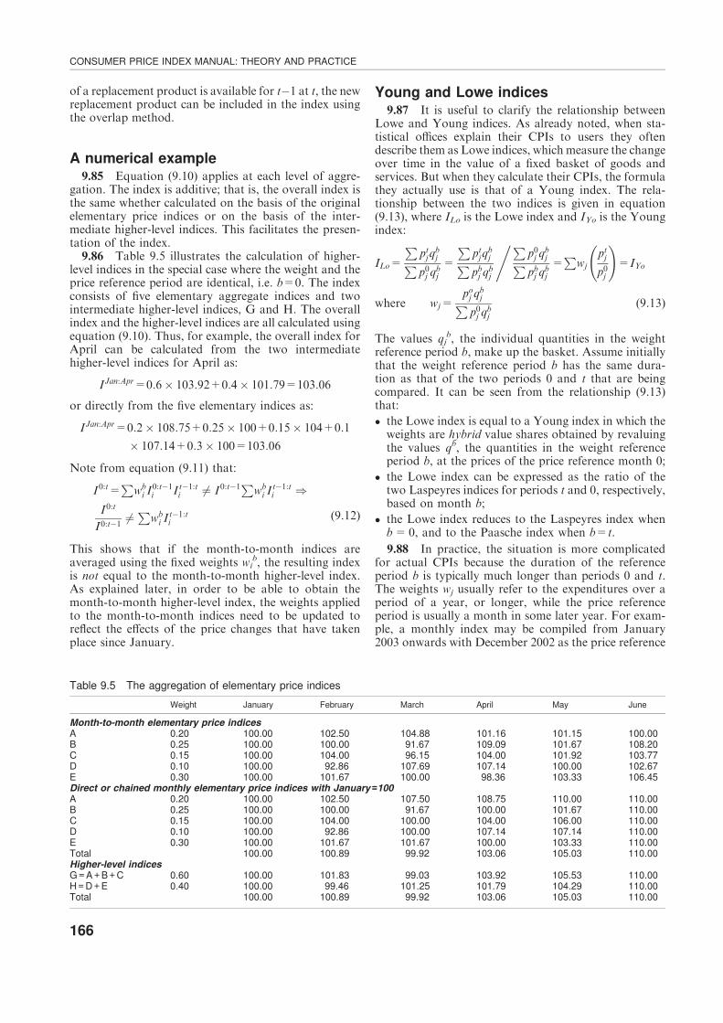
A numerical example9.85 Equation (9.10) applies at each level of aggre-

gation. The index is additive; that is, the overall index isthe same whether calculated on the basis of the originalelementary price indices or on the basis of the inter-mediate higher-level indices. This facilitates the presen-tation of the index.

9.86 Table 9.5 illustrates the calculation of higher-level indices in the special case where the weight and theprice reference period are identical, i.e. b=0. The indexconsists of five elementary aggregate indices and twointermediate higher-level indices, G and H. The overallindex and the higher-level indices are all calculated usingequation (9.10). Thus, for example, the overall index forApril can be calculated from the two intermediatehigher-level indices for April as:

IJan:Apr=0:6� 103:92+0:4� 101:79=103:06

or directly from the five elementary indices as:

IJan:Apr=0:2� 108:75+0:25� 100+0:15� 104+0:1

� 107:14+0:3� 100=103:06

Note from equation (9.11) that:

I0:t=P

wbi I

0:t�1i I t�1:t

i 6¼ I0:t�1Pwbi I

t�1:ti )

I0:t

I0:t�1 6¼P

wbi I

t�1:ti

(9.12)

This shows that if the month-to-month indices areaveraged using the fixed weights wi

b, the resulting indexis not equal to the month-to-month higher-level index.As explained later, in order to be able to obtain themonth-to-month higher-level index, the weights appliedto the month-to-month indices need to be updated toreflect the effects of the price changes that have takenplace since January.

Young and Lowe indices9.87 It is useful to clarify the relationship between

Lowe and Young indices. As already noted, when sta-tistical offices explain their CPIs to users they oftendescribe them as Lowe indices, which measure the changeover time in the value of a fixed basket of goods andservices. But when they calculate their CPIs, the formulathey actually use is that of a Young index. The rela-tionship between the two indices is given in equation(9.13), where ILo is the Lowe index and IYo is the Youngindex:

ILo=

Pptjq

bjP

p0j qbj

=

Pptjq

bjP

pbj qbj

,Pp0j q

bjP

pbj qbj

=P

wj

ptj

p0j

!=IYo

where wj=poj q

bjP

p0j qbj

(9.13)

The values qjb, the individual quantities in the weight

reference period b, make up the basket. Assume initiallythat the weight reference period b has the same dura-tion as that of the two periods 0 and t that are beingcompared. It can be seen from the relationship (9.13)that:

� the Lowe index is equal to a Young index in which theweights are hybrid value shares obtained by revaluingthe values qb, the quantities in the weight referenceperiod b, at the prices of the price reference month 0;

� the Lowe index can be expressed as the ratio of thetwo Laspeyres indices for periods t and 0, respectively,based on month b;

� the Lowe index reduces to the Laspeyres index whenb=0, and to the Paasche index when b=t.

9.88 In practice, the situation is more complicatedfor actual CPIs because the duration of the referenceperiod b is typically much longer than periods 0 and t.The weights wj usually refer to the expenditures over aperiod of a year, or longer, while the price referenceperiod is usually a month in some later year. For exam-ple, a monthly index may be compiled from January2003 onwards with December 2002 as the price reference

Table 9.5 The aggregation of elementary price indices

Weight January February March April May June

Month-to-month elementary price indicesA 0.20 100.00 102.50 104.88 101.16 101.15 100.00B 0.25 100.00 100.00 91.67 109.09 101.67 108.20C 0.15 100.00 104.00 96.15 104.00 101.92 103.77D 0.10 100.00 92.86 107.69 107.14 100.00 102.67E 0.30 100.00 101.67 100.00 98.36 103.33 106.45Direct or chained monthly elementary price indices with January=100A 0.20 100.00 102.50 107.50 108.75 110.00 110.00B 0.25 100.00 100.00 91.67 100.00 101.67 110.00C 0.15 100.00 104.00 100.00 104.00 106.00 110.00D 0.10 100.00 92.86 100.00 107.14 107.14 110.00E 0.30 100.00 101.67 101.67 100.00 103.33 110.00Total 100.00 100.89 99.92 103.06 105.03 110.00Higher-level indicesG=A+B+C 0.60 100.00 101.83 99.03 103.92 105.53 110.00H=D+E 0.40 100.00 99.46 101.25 101.79 104.29 110.00Total 100.00 100.89 99.92 103.06 105.03 110.00

CONSUMER PRICE INDEX MANUAL: THEORY AND PRACTICE

166

month, but the latest available weights during the year2003 may refer to the year 2000 or even some earlieryear.9.89 Conceptually, a typical CPI may be viewed as a

Lowe index that measures the change from month tomonth in the total cost of an annual basket of goods andservices that may date back several years before the pricereference period. Because it uses the fixed basket of anearlier period, it is sometimes loosely described as a‘‘Laspeyres-type index’’, but this description is unwar-ranted. A true Laspeyres index would require the basketto be that consumed in the price reference month,whereas in most CPIs the basket not only refers to adifferent period from the price reference month but to aperiod of a year or more. When the weights are annualand the prices are monthly, it is not possible, even retro-spectively, to calculate a monthly Laspeyres priceindex.9.90 As shown in Chapter 15, a Lowe index that

uses quantities derived from an earlier period than theprice reference period is likely to exceed the Laspeyres,and by a progressively larger amount, the further back intime the weight reference period is. The Lowe index islikely to have an even greater upward bias than theLaspeyres as compared with some target superlativeindex or underlying cost of living index. Inevitably, thequantities in any basket index become increasingly outof date and irrelevant the further back in time theperiod to which they relate. To minimize the result-ing bias, the weights should be updated as often aspossible.9.91 A statistical office may not wish to estimate a

cost of living index and may prefer to choose somebasket index as its target index. In that case, if the the-oretically attractive Walsh index were to be selected asthe target index, a Lowe index would have the same biasas just described, given that the Walsh index is also asuperlative index.

Factoring the Young index9.92 It is possible to calculate the change in a higher-

level Young index between two consecutive periods,such as t�1 and t, as a weighted average of the indivi-dual price indices between t�1 and t provided that theweights are updated to take account of the price changesbetween the price reference period 0 and the previousperiod, t�1. This makes it possible to factor the formula(9.10) into the product of two component indices in thefollowing way:

I0:t=I0:t�1Pwb(t�1)i I t�1:1

i

where wb(t�1)i =wb

i I0:t�1i

.Pwbi I

0:t�1i : (9.14)

I 0:t�1 is the Young index for period t�1. The weightwi

b(t�1) is the original weight for elementary aggregate iprice-updated by multiplying it by the elementary priceindex for i between 0 and t�1, the adjusted weightsbeing rescaled to sum to unity. The price-updatedweights are hybrid weights because they implicitlyrevalue the quantities of b at the prices of t�1 instead

of at the average prices of b. Such hybrid weights do notmeasure the actual expenditure shares of any period.

9.93 The index for period t can thus be calculated bymultiplying the already calculated index for t�1 by aseparate Young index between t�1 and t with hybridprice-updated weights. In effect, the higher-level index iscalculated as a chain index in which the index is movedforward period by period. This method gives more flex-ibility to introduce replacement items and makes it easierto monitor the movements of the recorded prices forerrors, as month-to-month movements are smaller andless variable than the total changes since the base period.

9.94 Price-updating may also occur between theweight reference period and the price reference period,as explained in the next section.

Price-updating from the weight referenceperiod to the price reference period

9.95 When the weight reference period b and theprice reference period 0 are different, as is normally thecase, the statistical office has to decide whether or not toprice-update the weights from b to 0. In practice, theprice-updated weights can be calculated by multiplyingthe original weights for period b by elementary indicesmeasuring the price changes between periods b and 0and rescaling to sum to unity.

9.96 The issues involved are best explained with thehelp of a numerical example. In Table 9.6, the baseperiod b is assumed to be the year 2000, so the weightsare the expenditure shares in 2000. In section (a) of Table9.6, 2000 is also used as the price reference period. Inpractice, however, weights based on 2000 cannot beintroduced until some time after 2000 because of the timeneeded to collect and process the expenditure data. Insection (b) of Table 9.6, it is assumed that the 2000weights are introduced in December 2002 and that this isalso chosen as the new price reference base.

9.97 Note that it would be possible in December2002 to calculate the indices based on 2000 shown insection (a) of the table, but it is decided to makeDecember 2002 the price reference base. This does notprevent the index with the December 2002 price referenceperiod from being calculated backwards a few monthsinto 2002, if desired.

9.98 The statistical office compiling the index hastwo options at the time the new index is introduced. It hasto decide whether the weights in the new index shouldpreserve the quantities in 2000 or the expenditures in2000. It cannot do both.

9.99 If it is decided to preserve the quantities, theresulting index is a basket index, or Lowe index, in whichthe quantities are those of the year 2000. This impliesthat the movements of the index must be identical withthose of the index based on 2000 shown in section (a) ofthe table. In this case, if the index is to be presented as aweighted average of the elementary price indices withDecember 2002 as the price reference period, theexpenditure weights for 2000 have to be price-updated toDecember 2002. This is illustrated in section (b) of Table9.6, where the updated weights are obtained by multi-plying the original weights for 2000 in section (a) of the

CALCULATING CONSUMER PRICE INDICES IN PRACTICE

167

table by the price indices for the elementary aggregatesbetween 2000 and December 2002, and then rescaling theresults to sum to unity. These are the weights labelledw00(Dec02) in the table.

9.100 The indices with price-updated weights insection (b) of Table 9.6 are Lowe indices in which b=2000 and 0=December 2002. These indices can beexpressed as ratios of the indices in the upper part of thetable. For example, the overall Lowe index for March2003 with December 2002 as its price reference base,namely 101.97, is the ratio of the index for March 2003based on 2000 shown in section (a) of the table, namely106.05, divided by the index for December 2002 based on2000, namely 104.00. Thus, the price-updating preservesthe movements of the indices in section (a) of the tablewhile shifting the price reference period to December2002.

9.101 Alternatively, it could be decided to calculate aseries of Young indices using the expenditure weightsfrom 2000 as they stand without updating. If theexpenditure shares were actually to remain constant,the quantities would have had to move inversely with theprices between 2000 and December 2002. The quantitiesthat make up the basket for the new Young index couldnot be the same as those of 2000. The movements of thisindex would have to be slightly different from those ofthe price-updated index.

9.102 The issue is whether to stick with the knownquantities of the weight reference period 2000, which arethe latest for which firm data have been collected, or tostick with the known expenditure shares of the weightreference period. If the official objective is to measure aLowe index that uses a fixed basket, the issue is decidedand the statistical office is obliged to price-update. On theother hand, some statistical offices may have to decidefor themselves which option to adopt.

9.103 Updating the prices without updating thequantities does not imply that the resulting expenditureweights are necessarily more up to date. When there is astrong inverse relation between movements of price andquantities, price-updating on its own could produceperverse results. For example, the prices of computershave been declining rapidly in recent years. If the quan-tities are held fixed while the prices are updated, theresulting expenditures on computers would also declinerapidly. In practice, however, the share of expendi-tures on computers might be actually be rising becauseof a very rapid increase in quantities of computerspurchased.

9.104 When there are rapid changes taking place inrelative quantities as well as relative prices, statisticaloffices are effectively obliged to change their expenditureweights more frequently, even if this means conductingmore frequent expenditure surveys. Price-updating onits own cannot cope with this situation. The expenditureweights have to be updated with respect to their quan-tities as well as their prices, which, in effect, impliescollecting new expenditure data.

The introduction of new weightsand chain linking

9.105 From time to time, the weights for the ele-mentary aggregates have to be revised to ensure thatthey reflect current expenditure patterns and consumerbehaviour. When new weights are introduced, the pricereference period for the new index can be the last periodof the old index, the old and the new indices being linkedtogether at this point. The old and the new indices makea chain index.

9.106 The introduction of new weights is often acomplex operation because it provides the opportunity

Table 9.6 Price-updating of weights between the weight and price reference periods

Weight 2000 Nov. 02 Dec. 02 Jan. 03 Feb. 03 Mar. 03

(a) Index with 2000 as weight and price reference periodElementary price indices

w00

A 0.20 100.00 98.00 99.00 102.00 101.00 104.00B 0.25 100.00 106.00 108.00 107.00 109.00 110.00C 0.15 100.00 104.00 106.00 98.00 100.00 97.00D 0.10 100.00 101.00 104.00 108.00 112.00 114.00E 0.30 100.00 102.00 103.00 106.00 105.00 106.00

Higher-level indicesG=A+B+C 0.60 100.00 102.83 104.50 103.08 104.08 104.75H=D+E 0.40 100.00 101.75 103.25 106.50 106.75 108.00Total 100.00 102.40 104.00 104.45 105.15 106.05(b) Index re-referenced to December 2002 and weights price-updated to December 2002

Elementary price indicesw00(Dec02)

A 0.190 101.01 98.99 100.00 103.03 102.02 105.05B 0.260 92.59 98.15 100.00 99.07 100.93 101.85C 0.153 94.34 98.11 100.00 92.45 94.34 91.51D 0.100 96.15 97.12 100.00 103.85 107.69 109.62E 0.297 97.09 99.03 100.00 102.91 101.94 102.91

Higher-level indicesG=A+B+C 0.603 95.69 98.41 100.00 98.64 99.60 100.24H=D+E 0.397 96.85 98.55 100.00 103.15 103.39 104.60Total 96.15 98.46 100.00 100.43 101.11 101.97Rescaled to 2000= 100 100.00 102.40 104.00 104.45 105.15 106.05

CONSUMER PRICE INDEX MANUAL: THEORY AND PRACTICE

168

to introduce new items, new samples, new data sources,new compilation practices, new elementary aggregates,new higher-level indices or new classifications. Thesetasks are often undertaken simultaneously at the time ofreweighting to minimize overall disruption to the timeseries and any resulting inconvenience to users of theindices.9.107 In many countries, reweighting and chaining

are carried out about every five years, but some countriesintroduce new weights each year. Chain indices do nothave to be linked annually; the linking may be done lessfrequently. The real issue is not whether to chain or notbut how frequently to chain. Reweighting is inevitablesooner or later, as the same weights cannot continueto be used for ever. Whatever the time frame, sta-tistical offices have to address the issue of chain linkingsooner or later. It is inevitable and a major task for indexcompilers.9.108 Frequency of reweighting. It is reasonable to

continue to use the same set of elementary aggregateweights so long as consumption patterns at the elemen-tary aggregate level remain fairly stable. Over time,consumers will tend to substitute away from products ofwhich the prices have increased relatively. Thus, in gen-eral, movements in prices and quantities tend to beinversely related. This kind of substitution behaviour onthe part of consumers implies that a Lowe index basedon the fixed basket of an earlier period will tend to havean upward bias compared with a basket index usingup-to-date weights.9.109 Another reason why consumption patterns

change is that new products are continually beingintroduced on the market while others drop out. Over thelonger term, consumption patterns are also influenced byseveral other factors. These include rising incomes andstandards of living, demographic changes in the structureof the population, changes in technology, and changes intastes and preferences.9.110 There is wide consensus that regular updating

of weights – at least every five years, and more often ifthere is evidence of rapid changes in consumption pat-terns – is a sensible and necessary practice. The questionof how often to change the weights and chain link theindex is nevertheless not straightforward, as frequentlinking can also have some disadvantages. It can becostly to obtain new weights, especially if they requiremore frequent expenditure surveys. Annual chaining hasthe advantage that changes (such as the inclusion of newgoods) can be introduced on a regular basis, althoughevery index needs some ongoing maintenance, whetherannually chained or not.9.111 Expenditures on certain types of products

are strongly influenced by short-term fluctuations inthe economy. For example, expenditures on cars, majordurables, expensive luxuries, and so on, may change dras-tically from year to year. In such cases, it may be pre-ferable to base the weight on an average of two or moreyears of expenditure.9.112 The calculation of a chain index. Assume that a

series of fixed weight Young indices has been calculatedwith period 0 as the price reference period and that in asubsequent period, k, a new set of weights has to be

introduced in the index. The new set of weights may, ormay not, have been price-updated from the new weightreference period to period k. A chain index is then cal-culated as:

I0:t=I0:kPwki I

k:t�1i I t�1:t

i

=I0:kPwki I

k:ti

=I0:kIk:t (9.15)

9.113 There are several important features of a chainindex:

� The chain index formula allows weights to be up-dated, and facilitates the introduction of new itemsand sub-indices and the removal of obsolete ones.

� In order to be able to link the old and the new series,an overlapping period (k) is needed in which the indexhas to be calculated using both the old and the new setof weights.

� A chain index may have two or more links. Betweeneach link period, the index may be calculated as afixed weight index using the formula (9.10), or indeedusing any other index formula. The link period maybe a month or a year, provided the weights and indicesrefer to the same period.

� Chaining is intended to ensure that the individualindices on all levels show the correct developmentthrough time.

� Chaining leads to non-additivity. When the newseries is chained onto the old, as in equation (9.15),the higher-level indices after the link cannot beobtained as weighted arithmetic averages of indivi-dual indices using the new weights. If, on the otherhand, the index reference period is changed and theindex series prior to the link period is rescaled to thenew index reference period, this series cannot beaggregated to higher-level indices by use of the newweights. Such results need to be carefully explainedand presented.

9.114 An example of the calculation of a chain indexis presented in Table 9.7. From 1998 to December 2002the index is calculated with the year 1998 as weight andprice reference period. From December 2002 onwards, anew set of weights is introduced. The weights may referto the year 2000, for example, and may or may not havebeen price-updated to December 2002. A new fixedweight index series is then calculated with December2002 as the price reference month. Finally, the new indexseries is linked onto the old index with 1998=100 bymultiplication to get a continuous index from 1998 toMarch 2003. The chained higher-level indices in Table9.7 are calculated as:

I00:t=I98:Dec02Pw00(Dec 02)i IDec 02:t

i (9.16)

Because of the lack of additivity, the overall chain indexfor March 2003 (129.07), for example, cannot be cal-culated as the weighted arithmetic mean of the chainedhigher-level indices G and H using the weights fromDecember 2002.

CALCULATING CONSUMER PRICE INDICES IN PRACTICE

169

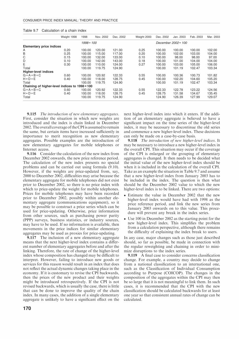
9.115 The introduction of new elementary aggregates.First, consider the situation in which new weights areintroduced and the index is chain linked in December2002.Theoverall coverageof theCPI isassumedto remainthe same, but certain items have increased sufficiently inimportance to merit recognition as new elementaryaggregates. Possible examples are the introduction ofnew elementary aggregates for mobile telephones orInternet access.

9.116 Consider the calculation of the new index fromDecember 2002 onwards, the new price reference period.The calculation of the new index presents no specialproblems and can be carried out using formula (9.10).However, if the weights are price-updated from, say,2000 to December 2002, difficulties may arise because theelementary aggregate for mobile telephones did not existprior to December 2002, so there is no price index withwhich to price-update the weight for mobile telephones.Prices for mobile telephones may have been recordedprior to December 2002, possibly within another ele-mentary aggregate (communications equipment), so itmay be possible to construct a price series which can beused for price-updating. Otherwise, price informationfrom other sources, such as purchasing power parity(PPP) surveys, business statistics, or industry sources,may have to be used. If no information is available, thenmovements in the price indices for similar elementaryaggregates may be used as proxies for price-updating.

9.117 The inclusion of a new elementary aggregatemeans that the next higher-level index contains a differ-ent number of elementary aggregates before and after thelinking. Therefore, the rate of change of the higher-levelindex whose composition has changed may be difficult tointerpret. However, failing to introduce new goods orservices for this reason would result in an index that doesnot reflect the actual dynamic changes taking place in theeconomy. If it is customary to revise the CPI backwards,then the prices of the new product and their weightsmight be introduced retrospectively. If the CPI is notrevised backwards, which is usually the case, there is littlethat can be done to improve the quality of the chainindex. In many cases, the addition of a single elementaryaggregate is unlikely to have a significant effect on the

next higher-level index into which it enters. If the addi-tion of an elementary aggregate is believed to have asignificant impact on the time series of the higher-levelindex, it may be necessary to discontinue the old seriesand commence a new higher-level index. These decisionscan only be made on a case-by-case basis.

9.118 The introduction of new higher-level indices. Itmay be necessary to introduce a new higher-level index inthe overall CPI. This situation may occur if the coverageof the CPI is enlarged or the grouping of elementaryaggregates is changed. It then needs to be decided whatthe initial value of the new higher-level index should bewhen it is included in the calculation of the overall CPI.Take as an example the situation in Table 9.7 and assumethat a new higher-level index from January 2003 has tobe included in the index. The question is then whatshould be the December 2002 value to which the newhigher-level index is to be linked. There are two options:

� Estimate the value in December 2002 that the newhigher-level index would have had with 1998 as theprice reference period, and link the new series fromJanuary 2003 onwards on to this value. This proce-dure will prevent any break in the index series.

� Use 100 in December 2002 as the starting point for thenew higher-level index. This simplifies the problemfrom a calculation perspective, although there remainsthe difficulty of explaining the index break to users.

In any case, major changes such as those just describedshould, so far as possible, be made in connection withthe regular reweighting and chaining in order to mini-mize disruptions to the index series.

9.119 A final case to consider concerns classificationchange. For example, a country may decide to changefrom a national classification to an international one,such as the Classification of Individual Consumptionaccording to Purpose (COICOP). The changes in thecomposition of the aggregates within the CPI may thenbe so large that it is not meaningful to link them. In suchcases, it is recommended that the CPI with the newclassification should be calculated backwards for at leastone year so that consistent annual rates of change can becalculated.

Table 9.7 Calculation of a chain index

Weight 1998 1998 Nov. 2002 Dec. 2002 Weight 2000 Dec. 2002 Jan. 2003 Feb. 2003 Mar. 2003

1998=100 December 2002=100Elementary price indicesA 0.20 100.00 120.00 121.00 0.25 100.00 100.00 100.00 102.00B 0.25 100.00 115.00 117.00 0.20 100.00 102.00 103.00 104.00C 0.15 100.00 132.00 133.00 0.10 100.00 98.00 98.00 97.00D 0.10 100.00 142.00 143.00 0.18 100.00 101.00 104.00 104.00E 0.30 100.00 110.00 124.00 0.27 100.00 103.00 105.00 106.00Total 100.00 119.75 124.90 100.00 101.19 102.47 103.34Higher-level indicesG=A+B+C 0.60 100.00 120.92 122.33 0.55 100.00 100.36 100.73 101.82H=D+E 0.40 100.00 118.00 128.75 0.45 100.00 102.20 104.60 105.20Total 100.00 119.75 124.90 100.00 101.19 102.47 103.34Chaining of higher-level indices to 1998=100G=A+B+C 0.60 100.00 120.92 122.33 0.55 122.33 122.78 123.22 124.56H=D+E 0.40 100.00 118.00 128.75 0.45 128.75 131.58 134.67 135.45Total 100.00 119.75 124.90 124.90 126.39 127.99 129.07

CONSUMER PRICE INDEX MANUAL: THEORY AND PRACTICE

170

9.120 Partial reweighting. The weights for the ele-mentary aggregates may be obtained from a variety ofsources over a number of different periods. Conse-quently, it may not be possible to introduce all the newweighting information at the same time. In some cases, itmay be preferable to introduce new weights for someelementary aggregates as soon as possible after theinformation is received. The introduction of new weightsfor a subset of the overall index is known as partialreweighting.9.121 Partial reweighting has particular implications

for the practice of price-updating the weights. Weightinginformation may not be available for some elementaryaggregates at the time of rebasing. Thus, it may benecessary to consider price-updating not only the newweights, but also the old weights for those elementaryaggregates for which no new weights are available. Theweights for the latter may have to be price-updated overa long period, which, for reasons given earlier, may giverise to serious problems if relative quantities havechanged inversely to the relative price changes. Data onboth quantity and price changes should be sought beforeundertaking such updates. The disadvantage of partialreweighting is that the implicit quantities belong todifferent periods, so that the composition of the basketis obscure and not well defined.9.122 It may be concluded that the introduction of

new weights and the linking of a new series to an oldseries is not difficult in principle. The difficulties arise inpractice when trying to align weight and price referenceperiods and when deciding whether higher-level indicescomprising different elementary aggregates should bechained over time. It is not possible for this manual toprovide specific guidance on decisions such as these, butcompilers should consider carefully the economic logicand statistical reliability of the resulting chained seriesand also the needs of users. In order to facilitate thedecision-making process, careful thought should begiven to these issues in advance during the planning of areweighting exercise, paying particular attention towhich of the indices are to be published.9.123 Long-term and short-term links. Consider a

long-term chain index in which the weights are changedannually. In any given year, the current monthly indicesare first calculated using the latest set of availableweights, which cannot be those of the current year.However, when the weights for the year in questionbecome available subsequently, the monthly indices canthen be recalculated on the basis of the weights forthat same year. The resulting series can then be used inthe long-term chain index, rather than the originalindices first published. Thus, the movements of thelong-term chain index from, say, any one December tothe following December are based on weights of thatsame year, the weights being changed each December.This method has been developed by the Central Statis-tical Office of Sweden, where it is applied in the calcu-lation of the CPI. It is described in Swedish ConsumerPrice Index: A Handbook of Methods (Statistics Sweden,2001).9.124 Assume that each link runs from December to

December. The long-term index for month m of year Y

with December of year 0 as index reference period isthen calculated using the formula:

IDec0:mY=YY�1y=1

IDecy�1:Decy

!IDecY�1:mY ð9:17Þ

=IDec 0:Dec1IDec1:Dec2 . . . IDecY�2:DecY�1IDecY�1:mY

In the actual Swedish practice, a factor scaling the indexfrom December year 0 to the average of year 0 is mul-tiplied onto the right-hand side of the formula (9.19) tohave a full year as the reference period. The long-termmovement of the index depends on the long-term linksonly, as the short-term links are successively replaced bytheir long-term counterparts. For example, let the short-term indices for January to December 2001 be calculatedas:

IDec 00:m01=P

w00(Dec 00)i IDec 00:m01

i (9.18)

where Wi00(Dec00) are the weights from 2000 price-

updated to December 2000. When weights for 2001become available, this is replaced by the long-term link:

IDec00:Dec01=P

w01(Dec 00)i IDec 00:Dec 01

i (9.19)

where Wi01(Dec00) are the weights from 2001 price-

backdated to December 2000. The same set of weightsfrom 2001 price-updated to December 2001 is used inthe new short-term link for 2002:

IDec01:m02=P

w01(Dec01)i IDec01:m02

i : (9.20)

9.125 Using this method, the movement of the long-term index is determined by contemporaneous weights.The method is conceptually attractive because the weightsthat are most relevant for most users are those based onconsumption patterns at the time the price changesactually take place. The method takes the process ofchaining to its logical conclusion, at least assuming theindices are not chained more frequently than once a year.As the method uses weights that are continually revised toensure that they are representative of current consumerbehaviour, the resulting index also largely avoids thesubstitution bias that occurs when the weights are basedon the consumption patterns of some period in the past.The method may therefore appeal to statistical officeswhose objective is to estimate a cost of living index.

9.126 Finally, it may be noted that the methodinvolves some revision of the index first published. Insome countries, there is opposition to revising a CPI onceit has been first published, although it is standard prac-tice for other economic statistics, including the nationalaccounts, to be revised as more information and moreup-to-date information become available. This point isconsidered further below.

Decomposition of index changes9.127 Users of the index are often interested in how

much of the change in the overall index is attributable tothe change in the price of some particular good or groupof products, such as oil or food. Alternatively, there may

CALCULATING CONSUMER PRICE INDICES IN PRACTICE

171

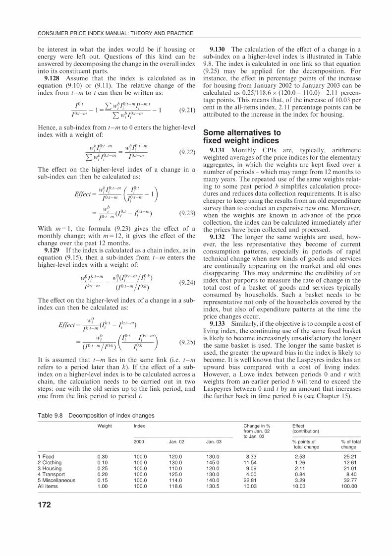
be interest in what the index would be if housing orenergy were left out. Questions of this kind can beanswered by decomposing the change in the overall indexinto its constituent parts.

9.128 Assume that the index is calculated as inequation (9.10) or (9.11). The relative change of theindex from t�m to t can then be written as:

I0:t

I0:t�m � 1=

Pwbi I

0:t�mi I t�m:t

iPwbi I

0:t�mi

� 1 (9.21)

Hence, a sub-index from t�m to 0 enters the higher-levelindex with a weight of:

wbi I

0:t�miP

wbi I

0:t�mi

=wbi I

0:t�mi

I0:t�m (9.22)

The effect on the higher-level index of a change in asub-index can then be calculated as:

Effect=wbi I

0:t�mi

I0:t�mI0:ti

I0:t�mi

� 1

� �

=wbi

I0:t�m (I0:ti � I0:t�m

i ) (9.23)

With m=1, the formula (9.23) gives the effect of amonthly change; with m=12, it gives the effect of thechange over the past 12 months.

9.129 If the index is calculated as a chain index, as inequation (9.15), then a sub-index from t�m enters thehigher-level index with a weight of:

w0i I

k:t�mi

Ik:t�m =w0i (I

0:t�mi

�I0:ki )

(I0:t�m�I0:k)

(9.24)

The effect on the higher-level index of a change in a sub-index can then be calculated as:

Effect=w0i

Ik:t�m (Ik:ti � Ik:t�m

i )

=w0i

(I0:t�m�I0:k)

I0:ti � I0:t�m

i

I0:ki

� �(9.25)

It is assumed that t�m lies in the same link (i.e. t�mrefers to a period later than k). If the effect of a sub-index on a higher-level index is to be calculated across achain, the calculation needs to be carried out in twosteps: one with the old series up to the link period, andone from the link period to period t.

9.130 The calculation of the effect of a change in asub-index on a higher-level index is illustrated in Table9.8. The index is calculated in one link so that equation(9.25) may be applied for the decomposition. Forinstance, the effect in percentage points of the increasefor housing from January 2002 to January 2003 can becalculated as 0.25/118.6� (120.0� 110.0)=2.11 percen-tage points. This means that, of the increase of 10.03 percent in the all-items index, 2.11 percentage points can beattributed to the increase in the index for housing.

Some alternatives tofixed weight indices

9.131 Monthly CPIs are, typically, arithmeticweighted averages of the price indices for the elementaryaggregates, in which the weights are kept fixed over anumber of periods – which may range from 12 months tomany years. The repeated use of the same weights relat-ing to some past period b simplifies calculation proce-dures and reduces data collection requirements. It is alsocheaper to keep using the results from an old expendituresurvey than to conduct an expensive new one. Moreover,when the weights are known in advance of the pricecollection, the index can be calculated immediately afterthe prices have been collected and processed.

9.132 The longer the same weights are used, how-ever, the less representative they become of currentconsumption patterns, especially in periods of rapidtechnical change when new kinds of goods and servicesare continually appearing on the market and old onesdisappearing. This may undermine the credibility of anindex that purports to measure the rate of change in thetotal cost of a basket of goods and services typicallyconsumed by households. Such a basket needs to berepresentative not only of the households covered by theindex, but also of expenditure patterns at the time theprice changes occur.

9.133 Similarly, if the objective is to compile a cost ofliving index, the continuing use of the same fixed basketis likely to become increasingly unsatisfactory the longerthe same basket is used. The longer the same basket isused, the greater the upward bias in the index is likely tobecome. It is well known that the Laspeyres index has anupward bias compared with a cost of living index.However, a Lowe index between periods 0 and t withweights from an earlier period b will tend to exceed theLaspeyres between 0 and t by an amount that increasesthe further back in time period b is (see Chapter 15).

Table 9.8 Decomposition of index changes

Weight Index Change in %from Jan. 02to Jan. 03

Effect(contribution)

2000 Jan. 02 Jan. 03 % points oftotal change

% of totalchange

1 Food 0.30 100.0 120.0 130.0 8.33 2.53 25.212 Clothing 0.10 100.0 130.0 145.0 11.54 1.26 12.613 Housing 0.25 100.0 110.0 120.0 9.09 2.11 21.014 Transport 0.20 100.0 125.0 130.0 4.00 0.84 8.405 Miscellaneous 0.15 100.0 114.0 140.0 22.81 3.29 32.77All items 1.00 100.0 118.6 130.5 10.03 10.03 100.00

CONSUMER PRICE INDEX MANUAL: THEORY AND PRACTICE

172

9.134 There are several possible ways of minimizingor avoiding the potential biases from the use of fixedweight indices. These are outlined below.9.135 Annual chaining. One way in which to mini-

mize the potential biases from the use of fixed-weightindices is obviously to keep the weights and the baseperiod as up to date as possible by frequent rebasing andchaining. Quite a number of countries have adopted thisstrategy and revise their weights annually. In any case, asnoted earlier, it would be impossible to deal with thechanging universe of products without some chaining ofthe price series within the elementary aggregates, even ifthe weights attached to the elementary aggregates remainfixed. Annual chaining eliminates the need to choose abase period, as the weight reference period is always theprevious year, or possibly the preceding year.9.136 Annual chaining with current weights. When the

weights are changed annually, it is possible to replace theoriginal weights based on the previous year, or years, bythose of the current year, if the index is revised retro-spectively as soon as information on the current year’sexpenditures becomes available. The long-term move-ments in the CPI are then based on the revised series.This is the method adopted by the Swedish StatisticalOffice, as explained above. This method could provideunbiased results.9.137 Other index formulae. When the weights are

revised less frequently, say every five years, anotherpossibility would be to use a different index formula forthe higher-level indices instead of an arithmetic averageof the elementary price indices. One possibility wouldbe a weighted geometric average. This is not subjectto the same potential upward bias as the arithmeticaverage. More generally, a weighted version of theLloyd–Moulton formula might be considered. This for-mula takes account of the substitutions that consumersmake in response to changes in relative prices, andshould be less subject to bias for this reason. It reduces tothe geometric average when the elasticity of substitutionis unity, on average. It is unlikely that such a formulacould replace the arithmetic average in the foreseeablefuture and gain general acceptance, if only because itcannot be interpreted as measuring changes in the valueof a fixed basket. It could, however, be compiled on anexperimental basis and might well provide a useful sup-plement to the main index. It could at least flag the extentto which the main index is liable to be biased and throwlight on its properties.9.138 Retrospective superlative indices. Finally, it is

possible to calculate a superlative index retrospectively.Superlative indices, such as Fisher and Tornqvist indices,treat both periods compared symmetrically and requireexpenditure data for both periods. Although the CPImay have to be some kind of Lowe index when it is firstpublished, it may be possible to estimate a superlativeindex later when much more information becomesavailable about consumers’ expenditures period by pe-riod. At least one office, the United States Bureau ofLabor Statistics, publishes such an index. The publica-tion of revised or supplementary CPIs raises mattersof statistical policy, although users readily accept revi-sions in other fields of economic statistics. Moreover,

users are already confronted with more than one CPI inthe European Union (EU) where the harmonized indexfor EU purposes may differ from the national CPI. Thusthe publication of supplementary indices which throwlight on the properties of the main index and which maybe of considerable interest to some users seems justifiedand acceptable.

Data editing9.139 This chapter has been concerned with the

methods used by statistical offices to calculate their CPIs.This concluding section considers the data editing car-ried out by statistical offices, a process that is very closelylinked to the calculation of the price indices for the ele-mentary aggregates. Data collection, recording andcoding – the data capture processes – are dealt with inChapters 5 to 7. The next step in the production of priceindices is data editing. Data editing is here meant tocomprise two steps:

– detection of possible errors and outliers;

– verifying and correction of data.

9.140 Logically, the purpose of detecting errors andoutliers is to exclude errors or outliers from the indexcalculation. Errors may be falsely reported prices, or theymay be caused by recording or coding mistakes. Also,missing prices because of non-response may be dealt withas errors. Possible errors and outliers are usually iden-tified as observations that fall outside some pre-specifiedacceptance interval or are judged to be unrealistic by theanalyst on some other ground. It may also be the case,however, that even if an observation is not identified as apotential error, it may actually show up to be false. Suchobservations are sometimes referred to as inliers. Some-times, by chance, the sampling may have captured anexceptional price change, which falls outside the accep-tance interval but has been verified as correct. In somediscussions of survey data, any extreme value is des-cribed as an outlier. The term is reserved here for extremevalues that have been verified as being correct.

9.141 When a possible error has been identified, itneeds to be verified whether it is in fact an error or not.This clarification can usually be made by asking therespondent to verify the price, or by comparison with theprice change of comparable items. If the value is in factan error, it needs to be corrected. This can be done easilyif the respondent can provide the correct price or, wherethis is not possible, by imputation or omitting the pricefrom the index calculation. If the value proves to becorrect, it should be included in the index. If it proves tobe an outlier, it can be accepted or corrected according toa pre-defined practice, e.g. omitting or imputation.

9.142 Although the power of computers providesobvious benefits, not all of these activities have to becomputerized. There should be a complete set of proce-dures and records that controls the processing of data,even though some or all of it may be undertaken withoutthe use of computers. It is not always necessary for all ofone step to be completed before the next is started. Ifthe process uses spreadsheets, for example, with defaultimputations predefined for any missing data, the index

CALCULATING CONSUMER PRICE INDICES IN PRACTICE

173

can be estimated and re-estimated whenever a newobservation is added or modified. The ability to examinethe impact of individual price observations on elemen-tary aggregate indices and the impact of elementaryindices on various higher-level aggregates is a usefulaid in all aspects of the computation and analyticalprocesses.

9.143 It is neither necessary nor desirable to applythe same degree of scrutiny to all reported prices. Theprice changes recorded by some respondents carry moreweight than others, and statistical analysts should beaware of this. For example, one elementary aggregatewith a weight of 2 per cent, say, may contain 10 prices,while another elementary aggregate of equal weight maycontain 100 prices. Obviously, an error in a reportedprice will have a much smaller effect in the latter, where itmay be negligible, while in the former it may cause asignificant error in the elementary aggregate index andeven influence higher-level indices.

9.144 There may be an interest in the individual ele-mentary indices, as well as in the aggregates built fromthem. Since the sample sizes used at the elementary levelmay often be small, any price collected, and error in it,may have a significant impact on the results for individualproducts or industries. The verification of reported datausually has to be done on an index-by-index basis, usingthe statistical analysts’ experience. Analysts will also needthe cooperation and support of the respondents to thesurvey to help explain unusual price movements.

9.145 Obviously, the design of the survey and ques-tionnaires also influences the occurrence of errors. Hence,price reports and questionnaires should be as clear andunambiguous as possible to prevent misunderstandingsand errors. Whatever the design of the survey, it isimportant to verify that the data collected are those thatwere requested initially. The survey questionnaire shouldprompt the respondent to indicate if the requested datacould not be provided. If, for example, a product is notproduced any more and thus is not priced in the currentmonth, a possible replacement would be requested alongwith details as to the extent of its comparability with theold one. In the event that a respondent cannot supply areplacement, there are a number of procedures for deal-ing with missing data (also discussed in Chapter 7).

Identifying possible errors and outliers9.146 One of the ways in which price surveys are

different from other economic surveys is that, althoughprices are recorded, the measurement concern is withprice changes. As the index calculations consist of com-paring the prices of matching observations from oneperiod to another, editing checks should focus on theprice changes calculated from pairs of observations,rather than on the reported prices themselves.

9.147 Identification of unusual price changes can beaccomplished by:

– non-statistical checking of input data;

– statistical checking of input data;

– output checking.

These will be described in turn.

9.148 Non-statistical checking of input data. Non-statistical checking can be undertaken by manuallychecking the input data, by inspection of the data pre-sented in comparable tables, or by setting filters.

9.149 When the price reports or questionnaires arereceived in the statistical office, the reported prices can bechecked manually by comparing these to the previouslyreported prices of the same items or by comparing themto prices of similar items from other outlets. While thisprocedure may detect obvious unusual price changes, it isfar from certain that all possible errors will be detected.It is also extremely time-consuming and, of course, itdoes not identify coding errors.

9.150 After the price data have been coded, the sta-tistical system can be programmed to present the data in acomparable tabular form. For example, a table showingthe percentage change for all reported prices from theprevious to the current month may be produced and usedfor detection of possible errors. Such tables may alsoinclude, for comparison, the percentage changes of pre-vious periods and 12-month changes. Most computerprograms and spreadsheets can easily sort the observa-tions according to, say, the size of the latest monthly rateof change, so that extreme values can easily be identified.It is also possible to group the observations by elementaryaggregates.

9.151 The advantage of grouping observations isthat it highlights potential errors so that the analyst doesnot have to look through all observations. A hierarchicalstrategy whereby all extreme price changes are firstidentified and then examined in context may save time,though the price changes underlying elementary aggre-gate indices, which have relatively high weights, shouldalso be examined in context.

9.152 Filtering is a method by which possible errors oroutliers are identified according to whether the pricechanges fall outside some predefined limits, such as plusor minus 20 per cent or even 50 per cent. This test shouldcapture any serious errors of data coding, as well as someof the cases where a respondent has erroneously reportedon a different product. It is usually possible to identifythese errors without reference to any other observations inthe survey, so this check can be carried out at the datacapture stage. The advantage of filtering is that it avoidsthe analyst having to look through a lot of individualobservations. The upper and lower limits may be set forthe latest monthly change, or change over some otherperiod. Again, they should take account of the contextof the price change, in that theymay be specified by item orelementary aggregates or higher-level indices. Largerchanges for items with prices that are known to be volatilemight be accepted without question. For example, formonthly changes, limits of plus or minus 10 per cent mightbe set for oil prices, while for professional services thelimits might be zero per cent to plus 5 per cent (as any pricethat falls is suspect), and for computers it might be �5 percent to zero per cent (as any price that rises is suspect).The limits can also be changed over time. If it is knownthat oil prices are rising, the limits could be 10 per cent to20 per cent, while if they are falling, the limits might be�10 per cent to �20 per cent. The count of failuresshould be monitored regularly to examine the limits. If too

CONSUMER PRICE INDEX MANUAL: THEORY AND PRACTICE

174

many observations are being identified for review, thelimits will need to be adjusted, or the scope refined.9.153 The use of automatic deletion systems is not

advised, however. It is a well-recorded phenomenon inpricing that price changes for many products, especiallydurables, are not undertaken smoothly over time, butsaved up to avoid what are termed ‘‘menu costs’’ asso-ciated with making a price change. These relatively sub-stantial increases may take place at different times fordifferent models of products and have the appearance ofextreme, incorrect values. To delete a price change foreach model of the product as being ‘‘extreme’’ at the timeit occurs is to ignore all price changes for the industry.9.154 Statistical checking of input data. Statistical

checking of input data compares, for some time period,each price change with the change in prices in the sameor a similar sample. Two examples of such filtering aregiven here, the first based on non-parametric summarymeasures and the second on the log normal distributionof price changes.9.155 The first method involves tests based on the

median and quartiles of price changes, so they are unaf-fected by the impact of any single ‘‘extreme’’ observa-tion. Define the median, first quartile and third quartileprice ratios as RM, RQ1, and RQ3, respectively. Then anyobservation with a price ratio that is more than a certainmultiple C of the distance between the median and thequartile is identified as a potential error. The basicapproach assumes that price changes are normally dis-tributed. Under this assumption, it is possible to estimatethe proportion of price changes that are likely to falloutside given bounds expressed as multiples of C. Undera normal distribution, RQ1 and RQ3 are equidistantfrom RM. Thus, if C is measured as RM� (RQ1+RQ3)/2,then 50 per cent of observations would be expected to liewithin plus or minus C from the median. From the tablesof the standardized normal distribution this is equivalentto about 0.7 times the standard deviation (s). If, forexample, C was set to 6, the distance implied is about 4sof the sample, so about 0.17 per cent of observationswould be identified this way. With C=4, the corre-sponding figures are 2.7s, or about 0.7 per cent ofobservations. If C=3, the distance is 2.02s, so about 4per cent of observations would be identified.9.156 In practice, most prices may not change each

month and the share of observations identified as possibleerrors as a percentage of all changes would be undulyhigh. Some experimentation with alternative values of Cfor different industries or sectors may be appropriate. Ifthis test is to be used to identify possible errors for furtherinvestigation, a relatively low value of C should be used.9.157 To use this approach in practice, three mod-

ifications should be made:

� First, to make the calculation of the distance from thecentre the same for extreme changes on the low side aswell as on the high side, a transformation of the ratiosshould be made. The transformed distance for theratio of one price observation i, Si, should be:

Si=1� RM=Ri if 0<Ri <RM and

Si=Ri=RM � 1 if Ri �RM:

� Second, if the price changes are grouped closely to-gether, the distances between the median and quartilesmay be very small, so that many observations wouldbe identified that had quite small price changes. Toavoid this, some minimum distance, say 5 per cent formonthly changes, should also be set.

� Third, with small samples the impact of one obser-vation on the distances between the median andquartiles may be too great. Because sample sizes forsome elementary indices are small, samples for similarelementary indices may need to be grouped together.

9.158 For a detailed presentation of this method, seeHidiroglou and Berthelot (1986). The method can beexpanded to also take into account the level of the prices.Thus, for example, a price increase from 100 to 110 willbe attributed a different weight from the weight attrib-uted to a price increase from 10 to 11.

9.159 An alternative method can be used if it isthought that the price changes may be distributed lognormally. To apply this method, the standard deviationof the log of all price changes in the sample (excludingunchanged observations) is calculated and a goodness offit test (w2) is undertaken to identify whether the dis-tribution is log normal. If the distribution satisfies thetest, all price changes outside two times the exponentialof the standard deviation are highlighted for furtherchecking. If the test rejects the log normal hypothesis,all the price changes outside three times the exponentialof the standard deviation are highlighted. The samecaveats mentioned before about clustered changes andsmall samples apply.

9.160 The second example is based on the Tukeyalgorithm. The set of price ratios is sorted and thehighest and lowest 5 per cent flagged for further atten-tion. In addition, having excluded the top and bottom 5per cent, exclude the price ratios that are equal to 1 (nochange). The arithmetic (trimmed) mean (AM) of theremaining price ratios is calculated. This mean is used toseparate the price ratios into two sets, an upper and alower one. The upper and lower ‘‘mid-means’’, that is,the means of each of these sets (AML, AMU), are thencalculated. Upper and lower Tukey limits (TL, TU) arethen established as the mean plus (minus) 2.5 times thedifference between the mean and the mid-means:

TU=AM+2:5 (AMU �AM)

TL=AM� 2:5 (AM�AML)

Then all those observations that fall above TU andbelow TL are flagged for attention.

9.161 This is a simpler method similar to that basedon the normal distribution. Since it excludes all cases ofno change from the calculation of the mean, it is unlikelyto produce limits that are very close to the mean, so thereis no need to set a minimum difference. Its success willalso depend on there being a large number of observa-tions on the set of changes being analysed. Again, it willoften be necessary to group observations from similarelementary indices. For any of these algorithms, thecomparisons can be made for any time periods, includingthe latest month’s changes or longer periods, in partic-ular, 12-month changes.

CALCULATING CONSUMER PRICE INDICES IN PRACTICE

175

9.162 The advantage of these two models of filteringcompared to the simple method of filtering is that foreach period the upper and lower limits are determined bythe data and hence are allowed to vary over the year,given that the analyst has decided on the value of theparameters entering the models. A disadvantage is that,unless the analyst is prepared to use approximationsfrom earlier experience, all the data have to be collectedbefore the filtering can be undertaken. Filters should beset tightly enough so that the percentage of potentialerrors that turn out to be real errors is high. As with allautomatic methods, the flagging of an unusual observa-tion is for further investigation, as opposed to automaticdeletion.

9.163 Checking by impact, or data output checking.Filtering by impact, or output editing, is based on cal-culating the impact that an individual price change hason an index to which it contributes. This index can be anelementary aggregate index, the total index, or someother aggregate index. The impact that a price changehas on an index is its percentage change times its effec-tive weight. In the absence of sample changes, the cal-culation is straightforward: it is the nominal (referenceperiod) weight, multiplied by the price relative, anddivided by the level of the index to which it is con-tributing. So the impact on the index I of the change ofthe price of product i from time t to t+1 is ±wi ( pt+1 /pt)/It where wi is the nominal weight in the base period.A minimum value for this impact can be set, so that allprice changes that cause an impact greater than thischange can be flagged for review. If index I is an ele-mentary index, then all elementary indices may bereviewed, but if I is an aggregative index, prices thatchange by a given percentage will be flagged or notdepending on how important the elementary index towhich they contribute is in the aggregate.

9.164 At the lowest level, the appearance and dis-appearance of products in the sample cause the effectiveweight of an individual price to change substantially.The effective weight is also affected if a price observationis used as an imputation for other missing observations.The evaluation of effective weights in each period ispossible, though complicated. As an aid to highlightingpotential errors, the nominal weights, as a percentage oftheir sum, will usually provide a reasonable approx-imation. If the impact of 12-month changes is requiredto highlight potential errors, approximations are theonly feasible filters to use, as the effective weights willvary over the period.

9.165 One advantage of identifying potential errorsin this way is that it focuses on the results. Anotheradvantage is that this form of filtering also helps theanalyst to describe the contributions to change in theprice indices. In fact, much of this kind of analysis isdone after the indices have been calculated, as the analystoften wishes to highlight those indices that have con-tributed the most to overall index changes. Sometimesthe analysis results in a finding that particular industrieshave a relatively high contribution to the overall pricechange, and that is considered unrealistic. The change istraced back to an error, but it may be late in the pro-duction cycle and jeopardize the schedule release date.

There is thus a case for identifying such unusual con-tributions as part of the data editing procedures. Thedisadvantage of this method is that an elementary index’schange may be rejected at that stage. It may be necessaryto over-ride the calculated index, though this shouldbe only a stopgap measure until the index sample isredesigned.

Verifying and correcting data9.166 Some errors, such as data coding errors, can be

identified and corrected easily. Ideally, these errors arecaught at the first stage of checking, before they need tobe viewed in the context of other price changes. Dealingwith other potential errors is more difficult. Many resultsthat fail a data check may be judged by the analyst to bequite plausible, especially if the data checking limits arebroad. Some potential failures may only be resolved bychecking the data with the respondent.

9.167 If a satisfactory explanation can be obtainedfrom the respondent, the data can be verified or cor-rected. If not, procedures may differ. Rules may be estab-lished that if a satisfactory explanation is not obtained,then the reported price is omitted from the index calcu-lation. Alternatively, it may be left to the analyst to makethe best judgement as to the price change. If an analystmakes a correction to some reported data without veri-fying it with the respondent, the change may subse-quently cause problems with the respondent. If therespondent is not told of the correction, the same errormay persist in the future. The correct action depends ona combination of confidence in the analysts, the revisionpolicy of the survey, and the degree of communicationwith respondents. Most statistical organizations do notwant to burden respondents unduly.

9.168 In many organizations, a disproportionateshare of activity is devoted to identifying and followingup potential errors. If this practice leads to little changein the results, as a result of most reports finally beingaccepted, then the ‘‘bounds’’ on what are consideredto be extreme values should be relaxed. More errorsare likely to be introduced by respondents failing toreport changes that occur than from wrongly reportingchanges, and the good will of respondents should not beunduly undermined.

9.169 Generally, the effort spent on identifyingpotential errors should not be excessive. Obvious mis-takes should be caught at the data capture stage. Thetime spent in identifying observations to query, unlessthey are highly weighted and excessive, is often betterspent treating those cases in the production cycle wherethings have changed – quality changes or unavailableprices – and reorganizing activities towards maintainingthe relevance of the sample, and checking for errors ofomission.

9.170 If the price observations are collected in a waythat prompts the respondent with the previously repor-ted price, the respondent may report the same price as amatter of convenience. This can happen even though theprice may have changed, or even when the particularproduct being surveyed is no longer available. As pricesfor many items do not change frequently, this kind of

CONSUMER PRICE INDEX MANUAL: THEORY AND PRACTICE

176

error is unlikely to be spotted by normal checks. Oftenthe situation comes to light when the contact at theresponding outlet changes and the new contact has dif-ficulty in finding something that corresponds to the pricepreviously reported. It is advisable, therefore, to keep arecord of the last time a particular respondent reporteda price change. When that time has become suspiciouslylong, the analyst should verify with the respondent thatthe price observation is still valid. What constitutes toolong will vary from product to product and the level ofoverall price inflation, but, in general, any price that hasremained constant for more than a year is suspect.9.171 Treatment of outliers. Detection and treatment

of outliers (extreme values that have been verified asbeing correct) is an insurance policy. It is based on thefear that a particular data point collected is exceptionalby chance, and that if there were a larger survey, or evena different one, the results would be less extreme. Thetreatment, therefore, is to reduce the impact of theexceptional observation, though not to ignore it as, afterall, it did occur. The methods to test for outliers are thesame as those used to identify potential errors by sta-tistical filtering, described above. For example, upperand lower bounds of distances from the median pricechange are determined. In this case, however, whenobservations are found outside those bounds, they maybe changed to be at the bounds or imputed by the rateof change of a comparable set of prices. This outlieradjustment is sometimes made automatically, on thegrounds that the analyst by definition has no additionalinformation on which to base a better estimate. Whilesuch automatic adjustment methods are employed, thismanual proposes caution in their use. If an elementaryaggregate is relatively highly weighted and has a rela-tively small sample, an adjustment may be made. Thegeneral prescription should be to include verified prices;the exception should be to dampen them.9.172 Treatment of missing price observations. It is

likely that not all the requested data will have beenreceived by the time the index needs to be calculated. Itis generally the case that missing data turn out to bedelayed. Sometimes, the respondent may report that aprice cannot be reported because neither the product,nor any similar substitute is being made any more.Sometimes, of course, what started apparently as a latereport becomes a permanent loss to the sample. Differ-ent actions need to be taken depending on whether thesituation is temporary or permanent.9.173 For temporarily missing prices, the most

appropriate strategy is to minimize the occurrence ofmissing observations. Survey reports are likely to come in

over a period of time before the indices need to be cal-culated. In many cases, they follow a steady routine; somerespondents will tend to file quickly, others typically willbe later in the processing cycle. An analyst should becomefamiliar with these patterns. A computerized data capturesystem can flag those reports that appear to be later thanusual, well before the processing deadline. Also, somedata are more important than others. Depending on theweighting system, some respondents may be particularlyimportant, and important products should be flagged asrequiring particular scrutiny.

9.174 For those reports for which no estimate can bemade, two basic alternatives are considered here (seeChapter 7 for a full range of approaches): imputation,preferably targeted, in which the missing price changeis assumed to be the same as some other set of pricechanges; or an assumption of no change, as the precedingperiod’s price is used. This latter procedure ignores thefact that some prices will prove to have changed, and ifprices are generally moving in one direction, this willmean that the change in the index will be understated.It is not advised. However, if the index is periodicallyrevised, this approach will lead to fewer subsequentrevisions than imputations, since for most products,prices do not generally change in any given period. Stand-ard imputation is to base the estimate of the missing priceobservation on the change of some similar group ofobservations.

9.175 There will be situations where the price ispermanently missing because the product no longerexists. As there is no replacement for the missing price,an imputation will have to be made for each period untileither the sample is redesigned or until a replacementcan be found. It is, therefore, more important than inthe case of temporarily missing reports, and requirescloser attention.

9.176 The missing price can be imputed by using thechange in the remaining price observations in the ele-mentary aggregate, which has the same effect as remov-ing the missing observation from the sample, or by thechange in a subset of other price observations for com-parable items. The series should be flagged as beingbased on imputed values.

9.177 Samples are designed on the basis that theproducts chosen for observation are representative of awider range of products. Imputations for permanentlymissing prices are indications of weakness in the sample,and their accumulation is a signal that the sample shouldbe redesigned. For indices where there are known to be alarge number of disappearances in the sample, the needfor replacements should be anticipated.

CALCULATING CONSUMER PRICE INDICES IN PRACTICE

177