Calculation of Moon Phases and 24 Solar Terms

Yuk Tung Liu (廖育棟)

First draft: 2018-10-24, Last major revision: 2018-12-03

Chinese Versions: 傳傳傳統統統中中中文文文 简简简体体体中中中文文文

This document explains the method used to compute the times of the moon phases and 24solar terms. These times are important in the calculation of the Chinese calendar. See this pagefor an introduction to the 24 solar terms, and this page for an introduction to the Chinese calendarcalculation.

Computation of accurate times of moon phases and 24 solar terms is complicated, but todayall the necessary resources are freely available. Anyone familiar with numerical computation andcomputer programming can follow the procedure outlined in this document to do the computation.

Before stating the procedure, it is useful to have a basic understanding of the basic conceptsbehind the computation. I assume that readers are already familiar with the important astronomyconcepts mentioned on this page. In Section 1, I briefly introduce the barycentric dynamical time(TDB) used in modern ephemerides, and its connection to terrestrial time (TT) and internationalatomic time (TAI). Readers who are not familiar with general relativity do not have to pay muchattention to the formulas there. Section 2 introduces the various coordinate systems used inmodern astronomy. Section 3 lists the formulas for computing the IAU 2006/2000A precessionand nutation matrices.

One important component in the computation of accurate times of moon phases and 24 solarterms is an accurate ephemeris of the Sun and Moon. I use the ephemerides developed by theJet Propulsion Laboratory (JPL) for the computation. Section 4 introduces the JPL ephemeridesand describes how they can be downloaded and used to compute the positions and velocities ofsolar system objects. One of the main goals of the JPL ephemerides is for spacecraft navigation.Positions and velocities of the solar system objects are given in the international celestial referencesystem (ICRS). Hence, these data need to be transformed to the ecliptic coordinate system suitablefor the computation of the moon phases and 24 solar terms. Section 5 describes the light-timecorrection and aberration of light. Section 6 provides a step-by-step procedure for computingthe apparent geocentric longitude of the Sun and Moon from the data computed from the JPLephemerides. Section 7 describes the numerical method for computing the TDB times of the moonphases and 24 solar terms from the apparent geocentric longitudes of the Sun and Moon. Finally,Section 8 describes the conversion of times between TDB and UTC+8 necessary for calendarcalculation. For a more detailed and comprehensive introduction to the concepts mentioned inthis document, I recommend the book Explanatory Supplement to the Astronomical Almanac by[Urban & Seidelmann 2013].

1

1 Ephemeris Time and Barycentric Dynamical Time

From the 17th century to the late 19th century, planetary ephemerides were calculated usingtime scales based on Earth’s rotation. It was assumed that Earth’s rotation was uniform. Asthe precision of astronomical measurements increased, it became clear that Earth’s rotation is notuniform. Ephemeris time (ET) was introduced to ensure a uniform time for ephemeris calculations.It was defined by the orbital motion of the Earth around the Sun instead of Earth’s spin motion.However, a more precise definition of times is required when general relativistic effects need to beincluded in ephemeris calculations.

In general relativity, the passage of time measured by an observer depends on the spacetimetrajectory of the observer. To calculate the motion of objects in the solar system, the mostconvenient time is a coordinate time, which does not depend on the motion of any object but isdefined through the spacetime metric. In the Barycentric Celestial Reference System (BCRS), thespacetime coordinates are (t, xi) (i = 1, 2, 3). Here the time coordinate t is called the barycentriccoordinate time (TCB). The spacetime metric for the solar system can be written as [see Eq. (2.38)in [Urban & Seidelmann 2013]]

ds2 = −(

1− 2w

c2+

2w2

c4

)d(ct)2 − 4wi

c3d(ct)dxi + δij

[1 +

2w

c2+O(c−4)

]dxidxj, (1)

where sum over repeated indices is implied. The scalar potential w reduces to the Newtoniangravitational potential −Φ in the Newtonian limit, where

Φ(t,x) = −G∫d3x′

ρ(t,x′)

|x− x′|(2)

and ρ is the mass density. The vector potential wi satisfies the Poisson equations with the sourceterms proportional to the momentum density.

TCB can be regarded as the proper time measured by an observer far away from the solarsystem and is stationary with respect to the solar system barycenter. The equations of motion forsolar system objects can be derived in the post-Newtonian framework. The result is a system ofcoupled differential equations and can be integrated numerically. In this framework, TCB is thenatural choice of time parameter for planetary ephemerides. However, since most measurementsare carried out on Earth, it is also useful to set up a coordinate system with origin at the Earth’scenter of mass. In the geocentric celestial reference system (GCRS), the spacetime coordinatesare (T,X i), where the time parameter T is called the geocentric coordinate time (TCG). GCRS iscomoving with Earth’s center of mass in the solar system, and its spatial coordinates X i are chosento be kinematically non-rotating with respect to the barycentric coordinates xi. The coordinatetime TCG is chosen so that the spacetime metric has a form similar to equation (1). Since GCRSis comoving with the Earth, it is inside the potential well of the solar system. As a result, TCGelapses slower than TCB because of the combined effect of gravitational time dilation and specialrelativistic time dilation. The relation between TCB and TCG is given by [equation (3.25) in[Urban & Seidelmann 2013]]

TCB− TCG = c−2

[∫ t

t0

(v2e

2− Φext(xe)

)dt+ ve · (x− xe)

]+O(c−4), (3)

where xe and ve are the barycentric position and velocity of the Earth’s center of mass, and x isthe barycentric position of the observer. The external potential Φext is the Newtonian gravitational

2

potential of all solar system bodies apart from the Earth. The constant time t0 is chosen so thatTCB=TCG=ET at the epoch 1977 January 1, 0h TAI.

Since the definition of TCG involves only external gravity, TCG’s rate is faster than TAI’sbecause of the relativistic time dilation caused by Earth’s gravity and spin. The terrestrial time(TT), formerly called the terrestrial dynamical time (TDT), is defined so that its rate is the sameas the rate of TAI. The rate of TT is slower than TCG by −Φeff/c

2 on the geoid (Earth surface atmean sea level), where Φeff = ΦE − v2

rot/2 is the sum of Earth’s Newtonian gravitational potentialand the centrifugal potential. Here vrot is the speed of Earth’s spin at the observer’s location.The value of Φeff is constant on the geoid because the geoid is defined to be an equipotentialsurface of Φeff . Thus, dTT/dTCG = 1− LG and LG is determined by measurements to be LG =6.969290134×10−10. Therefore, TT and TCG are related by a linear relationship [equation (3.27)in [Urban & Seidelmann 2013]]:

TT = TCG− LG(JDTCG − 2443144.5003725) · 86400 s, (4)

where JDTCG is TCG expressed as a Julian date (JD). The constant 2443144.5003725 is chosenso that TT=TCG=ET at the epoch 1977 January 1 0h TAI (JD = 2443144.5003725). Since therate of TT is the same as that of TAI, the two times are related by a constant offset:

TT = TAI + 32.184 s. (5)

The offset arises from the requirement that TT match ET at the chosen epoch.TCB is a convenient time for planetary ephemerides, whereas TT can be measured directly by

atomic clocks on Earth. The two times are related by equations (3) and (4) and must be computedby numerical integration together with the planetary positions. TT is therefore not convenient forplanetary ephemerides. The barycentric dynamical time (TDB) is introduced to approximate TT.It is defined to be a linear function of TCB and is set as close to TT as possible. Since the rates ofTT and TCB are different and are changing with time, TT cannot be written as a linear functionof TCB. The best we can do is to set the rate of TDB the same as the rate of TT averaged overa certain time period, so that there is no long-term secular drift between TT and TDB over thattime period. The resulting deviation between TDB and TT has components of periodic variationcaused by the eccentricity of Earth’s orbit and the gravitational fields of the Moon and planets.TDB is now defined by the IAU 2006 resolution 3 as

TDB = TCB− LB(JDTCB − 2443144.5003725) · 86400 s− 6.55× 10−5 s, (6)

where LB = 1.550519768× 10−8 and JDTCB is TCB expressed as a Julian date (JD). The value ofLB can be regarded as 1− dTT/dt averaged over a certain time period.

TDB is a successor of ET as the time standard used by modern high-precision ephemerides. Therelationship between TT and TDB can be written as (Figure 3.2 in [Urban & Seidelmann 2013]]

TDB = TT + 0.001658s sin(g + 0.0167 sin g)+ lunar and planetary terms of order 10−5 s+ daily terms of order10−6 s, (7)

where g is the mean anomaly of Earth in its orbit (and hence g + 0.0167 sin g is the approximatevalue of the eccentric anomaly since 0.0167 is Earth’s orbital eccentricity). A more detailedexpression is given by equation (2.6) in [Kaplan 2005]. The difference between TDB and TTremains under 2 ms for several millennia around the present epoch. Thus, I treat them as thesame for the calendar calculation.

3

2 Celestial Coordinate Systems

2.1 International Celestial Reference System (ICRS)

As mentioned in Section 1, the solar system metric can be written in the Barycentric CelestialReference System (BCRS). The origin of the BCRS spatial coordinates is at the solar systembarycenter, i.e. the center of mass of the solar system. However, BCRS is a dynamical concept.The statement of “we use BCRS” in general relativity is equivalent to the statement “we usebarycentric inertial coordinates” in Newtonian mechanics. BCRS does not define the orientationof the coordinate axes.1

The International Celestial Reference System (ICRS) is a kinematical concept. Its origin is atthe solar system barycenter. The ICRS axes are intended to be fixed with respect to space. Theyare determined based on hundreds of extra-galactic radio sources, mostly quasars, distributedaround the sky. The ICRS axes are aligned with the equatorial system based on the J2000.0 meanequator and equinox (see below) to within 17.3 milliarcseconds. The x-axis of the ICRS points inthe direction of the mean equinox of J2000.0. The z-axis points very close to the mean celestialnorth pole of J2000.0, and the y-axis is 90 to the east of the x-axis on the ICRS equatorial plane.So the ICRS is a right-handed rectangular coordinate system. ICRS can be transformed to theequatorial system of J2000.0 by the frame bias matrix, which will be discussed below.

It is assumed that those distant extra-galactic radio sources do not rotate with respect toasymptotically flat reference systems like BCRS. In principle this assumption should be checkedby testing if the motion of the solar system objects is compatible with the equation of motionbased on BCRS, with no Coriolis and centrifugal forces. So far no deviations have been noticed.

However, it is expected that the extra-galactic radio sources should show a secular aberrationdrift caused by the rotation of the solar system barycenter around the center of Milky Way, andthis drift was detected by analyzing decades of the very long baseline interferometry (VLBI) data([Titov, Lambert & Gontier 2011]). The magnitude of the drift is about 6 micro arcseconds peryear, which agrees with the prediction. This effect will need to be taken into account in the futureas measurement accuracies continue to improve.

2.2 Geocentric Celestial Reference System (GCRS)

The origin of Geocentric Celestial Reference System (GCRS) is at the center of mass of the Earth.Ignoring general relativistic correction, the GCRS spatial coordinates X i are related to the BCRSspatial coordinates xi by

X i = xi − xiE +O((vE/c)2), (8)

where xiE are the BCRS coordinates of Earth’s center of mass. Relativistic correction adds termsof order (vE/c)

2 ∼ 10−8 = 0.002′′. The Sun moves along the ecliptic with a rate of about 0.04′′

per second. The Moon moves faster, with a rate of about 0.5′′ per second. Thus ignoring (vE/c)2

correction will lead to an error of about 0.05 seconds in the computation of the times of 24 solarterms and about 0.004 seconds in the times of moon phases. These errors are much smaller thanthe one-second accuracy required by the official document [GB/T 33661-2017].

Like BCRS’s situation, the orientation of GCRS’s axes are unspecified. Here I adopt therecommendaton of IAU 2006 Resolution B2: the axes of BCRS are oriented according to the ICRS

1IAU 2006 Resolution B2 recommends that the BCRS definition is completed with the following: “For allpractical applications, unless otherwise stated, the BCRS is assumed to be oriented according to the ICRS axes.The orientation of the GCRS is derived from the ICRS-oriented BCRS.”

4

axes. Since GCRS’s spatial coordinates are defined to be non-rotating with respect to BCRS’sspatial coordinates and the (vE/c)

2 terms are neglected, GCRS’s axes can also be regarded asbeing aligned with the ICRS axes.

2.3 Equatorial and Ecliptic Coordinate Systems

The orientation of the coordinate axes described above are fixed in space. This is convenient fordescribing the positions of stars and planets. However, observations are made on Earth and hencecoordinate systems with axes defined by Earth’s spin or defined by Earth’s orbital plane are oftenused to describe positions of celestial objects. The coordinate systems whose axes are defined byEarth’s spin are called the equatorial coordinate systems, and the coordinate system whose axesare defined by Earth’s orbital plane are called the ecliptic coordinate systems.

2.3.1 Equator, Ecliptic and Equinoxes

The Celestial Intermediate Pole (CIP) is the mean rotation axis of the Earth whose motion inspace contains aperiodic components as well as periodic components with periods greater thantwo days. The motion of CIP is described by precession and nutation (see below).

The true equator is defined to be the plane perpendicular to the CIP that passes throughEarth’s center of mass. Thus, the true equator is constantly changing as a result of precession andnutation. The mean equator is the moving equator whose motion is prescribed only by precession.

Ecliptic generally refers to Earth’s orbital plane projected onto the celestial sphere. However,Earth’s orbital plane is changing because of planetary perturbation. To reduce uncertainties inthe definition of the ecliptic, the International Astronomical Union (IAU) have recommended thatthe ecliptic be defined as the plane perpendicular to the mean orbital angular momentum vectorof the Earth-Moon barycenter passing through the Sun in the BCRS.

Equator and ecliptic intercepts at two points, called the vernal equinox and autumnal equinox.The true equinoxes are the two points at which the true equator and ecliptic intercepts. The meanequinoxes are the two points at which the mean equator and ecliptic intercepts.

2.3.2 Precession, Nutation and Polar Motion

Earth’s spin axis changes its orientation in space because of luni-solar and planetary torques onthe oblate Earth. Earth’s spin axis also moves relative to the crust. This is called the polar motion.

The motion of Earth’s spin axis is composed of precession and nutation. Precession is the com-ponents that are aperiodic or have periods longer than 100 centuries. Nutation is the componentsthat are of shorter periods and its magnitude is much smaller. Motion with periods shorter thantwo days cannot be distinguished from components of polar motion arising from the tidal defor-mation of the Earth. They are considered as components of polar motion. Therefore, nutation isdefined as the periodic components in the motion of Earth’s spin axis with periods longer thantwo days but shorter than about 100 centuries.

The major component of precession is the rotation of Earth’s spin axis about the ecliptic polewith a period of about 26,000 years. This causes the vernal equinox to move westward by 50.3′′

per year. The principal period of nutation is 18.6 years, which is caused by the Moon’s orbitalplane precessing around the ecliptic. The amplitude of nutation is about 9′′. The amplitude ofthe polar motion is about 0.3′′. Apart from the above mentioned component caused by the tidaldeformation of the Earth, there are other components of polar motions, including a 433-day cycle

5

component called the Chandler wobble. Polar motion is not relevant in the calculation of moonphases and 24 solar terms because they are not defined using positions relative to a station onEarth’s surface but defined by the geocentric positions, i.e. positions relative to Earth’s center ofmass.

In addition to the precession of Earth’s spin axis, the orbital plane of the Earth-Moon systemaround the Sun also moves slowly because of planetary perturbation. Hence the ecliptic movesslowly in space. This is called the precession of the ecliptic, to be distinguished from the precessionof the equator2.

2.3.3 Equatorial “Of Date” Coordinates

Equatorial coordinates are based on the equator and equinox. The x-axis points to the vernalequinox. The y-axis lies in the equatorial plane and is 90 to the east of the x-axis. The z-axispoints to the celestial pole. Since equator and equinoxes are moving, an epoch must be specified(e.g. J2000.0) to the coordinate system.

One commonly used equatorial coordinate system is based on the mean equator and equinox ofJ2000.0 (i.e. mean equator and equinox at TDB noon on January 1, 2000). As mentioned above,there is a small misalignment between the coordinate axes of the ICRS and the axes of the J2000.0mean equatorial system. The coordinates in the two systems are related by the frame bias matrixB. Let xICRS denotes a column vector representing the ICRS coordinates and x2000 denotes acolumn vector representing coordinates of J2000.0 mean equatorial system. Then

x2000 = BxICRS. (9)

The frame bias matrix is given by Equation (4.4) in [Urban & Seidelmann 2013]:

B =

1− 12(dα2

0 + ξ20) dα0 −ξ0

−dα0 − η0ξ0 1− 12(dα2

0 + η20) −η0

ξ0 − η0dα0 η0 + ξ0dα0 1− 12(η2

0 + ξ20)

, (10)

where dα0 = −14.6 milliarcseconds, ξ0 = −16.617 milliarcseconds, and η0 = −6.8192 milliarcseconds.All of them have to be converted to radians. Substituting the numbers to the formula gives

B =

0.99999999999999425 −7.078279744× 10−8 8.05614894× 10−8

7.078279478× 10−8 0.99999999999999695 3.306041454× 10−8

−8.056149173× 10−8 −3.306040884× 10−8 0.999999999999996208

. (11)

To convert x2000 to the coordinates with repect to the true equator and equinox of date requiresthe multiplication of the precession matrix P (t) and nutation matrix N (t):

xeq = N (t)P (t)x2000 = N (t)P (t)BxICRS. (12)

The formulas for P (t) and N (t) will be given in Section 3 below.

2Precession of the equator was formerly called the luni-solar precession, and precession of the ecliptic wasformerly called the planetary precession. They are renamed because the terminologies are misleading. Planetaryperturbation also contributes to the precession of the equator, although the magnitude is much smaller.

6

2.3.4 Ecliptic “Of Date” Coordinates

The calculation of the times of moon phases and 24 solar terms requires the positions of the Sunand Moon in ecliptic coordinates of date. The ecliptic coordinate systems are based on the eclipticand equinox. The x-axis points to the direction of the vernal equinox. The y-axis lies in the eclipticplane and is 90 to the east of the x-axis. The z-axis points to the ecliptic pole. Therefore, theecliptic coordinates are related to the equatorial coordinates by a rotation about the x-axis byan angle ε, which is called the obliquity of the ecliptic and is the angle between the ecliptic poleand the CIP. Note that ε = ε(t) is a function of time because of precession and nutation. Thevalue of ε can be computed by equation (30) below. Let xeq be the column vector representingthe equatorial coordinates with respect to the true equator and equinox of date, and xec be thecolumn vector representing the ecliptic coordinates with respect to the ecliptic and true equinoxof date. Then

xec = R1(ε(t))xeq = R1(ε(t))N (t)P (t)BxICRS, (13)

where the rotation matrix is

R1(ε(t)) =

1 0 00 cos ε(t) sin ε(t)0 − sin ε(t) cos ε(t)

. (14)

The ecliptic longitude λ is defined as arg(xec + iyec), where arg(z) denotes the argument of thecomplex number z. In other words, λ = tan−1(yec/xec) with the angle in the appropriate quadrant.In many programming languages, there is an arctangent function (e.g. atan2 in FORTRAN, Cand python) that returns the angle in the correct quadrant.

3 Precession and Nutation

3.1 Precession Matrix

Denote X = (X Y Z)T the equatorial coordinates based on the mean equator and equinox atTDB time t and X0 = (X0 Y0 Z0)T the equatorial coordinates based on the mean equator andequinox at J2000.0, where the superscript T denotes transpose. So X and X0 are column vectors,and they are related by a 3D rotation described by the precession matrix P (t):

X = P (t)X0. (15)

In August 2006, the 26th General Assembly for the International Astronomical Union passeda resolution recommending that the P03 precession theory of [Capitaine et al 2003] be used forthe precession matrix. This model is referred to as the IAU 2006 precession theory. According tothis theory, the precession matrix is given by

P (t) = R3(χA)R1(−ωA)R3(−ψA)R1(ε0), (16)

where the rotation matrix R1 is given by equation (14) above and the rotation matrix R3 is givenby

R3(θ) =

cos θ sin θ 0− sin θ cos θ 0

0 0 1

. (17)

7

The angle ε0 = 84381.406′′ is the inclination angle between the J2000.0 ecliptic and J2000.0 meanequator. The angles ψA, ωA and χA can be found in equation (5.7) in [Kaplan 2005]or (5.39) and(5.40) in [IERS Conventions 2010]. They are given by

ψA = 5038.481507′′T − 1.0790069′′T 2 − 0.00114045′′T 3 + 0.000132851′′T 4 − 9.51′′ × 10−8T 5

ωA = 84381.406′′ − 0.025754′′T + 0.0512623′′T 2 − 0.00772503′′T 3 − 4.67′′ × 10−7T 4

+3.337′′ × 10−7T 5 (18)

χA = 10.556403′′T − 2.3814292′′T 2 − 0.00121197′′T 3 + 0.000170663′′T 4 − 5.60′′ × 10−8T 5,

where T = (JD − 2451545)/36525 is the Julian century from J2000.0 and JD is the TDB Juliandate number. The result of the matrix multiplication in equation (16) is also written out explicitlyin equation (5.10) in [Kaplan 2005]:

P11(t) = C4C2 − S2S4C3

P12(t) = C4S2C1 + S4C3C2C1 − S1S4S3

P13(t) = C4S2S1 + S4C3C2S1 + C1S4S3

P21(t) = −S4C2 − S2C4C3

P22(t) = −S4S2C1 + C4C3C2C1 − S1C4S3 (19)

P23(t) = −S4S2S1 + C4C3C2S1 + C1C4S3

P31(t) = S2S3

P32(t) = −S3C2C1 − S1C3

P33(t) = −S3C2S1 + C3C1

where

S1 = sin ε0 C1 = cos ε0S2 = sin(−ψA) C2 = cos(−ψA) (20)

S3 = sin(−ωA) C3 = cos(−ωA)S4 = sinχA C4 = cosχA

3.2 Nutation Matrix

Nutation is computed according to the IAU 2000A Theory of Nutation with slight IAU 2006adjustments. To construct the nutation matrix N (t), we need to first compute the following 14arguments given by equations (5.43) and (5.44) in [IERS Conventions 2010].

F1 ≡ l = Mean Anomaly of the Moon= 134.96340251 + 1717915923.2178′′T + 31.8792′′T 2

+0.051635′′T 3 − 0.00024470′′T 4

F2 ≡ l′ = Mean Anomaly of the Sun= 357.52910918 + 129596581.0481′′T − 0.5532′′T 2

+0.000136′′T 3 − 0.00001149′′T 4

F3 ≡ = L− Ω = Mean Longitude of the Moon− Ω= 93.27209062 + 1739527262.8478′′T − 12.7512′′T 2

−0.001037′′T 3 + 0.00000417′′T 4 (21)

8

F4 ≡ D = Mean Elongation of the Moon from the Sun= 297.85019547 + 1602961601.2090′′T − 6.3706′′T 2

+0.006593′′T 3 − 0.00003169′′T 4

F5 ≡ Ω = Mean Longitude of the Ascending Node of the Moon= 125.04455501 − 6962890.5431′′T + 7.74722′′T 2

+0.007702′′T 3 − 0.00005939′′T 4

The rest of the arguments are the mean longitudes of the 8 planets and general precession. Theyare given in radians as

F6 ≡ LMercury = 4.402608842 + 2608.7903141574T

F7 ≡ LVenus = 3.176146697 + 1021.3285546211T

F8 ≡ LEarth = 1.753470314 + 628.3075849991T

F9 ≡ LMars = 6.203480913 + 334.0612426700T

F10 ≡ LJupiter = 0.599546497 + 52.9690962641T (22)

F11 ≡ LSaturn = 0.874016757 + 21.3299104960T

F12 ≡ LUranus = 5.481293872 + 7.4781598567T

F13 ≡ LNeptune = 5.311886287 + 3.8133035638T

F14 ≡ pA = 0.02438175T + 0.0000538691T 2

Next, the nutation in longitude ∆ψ and nutation in obliquity ∆ε are given by the expressions

∆ψ =1320∑i=1

[Ai sin θAi + A′′i cos θAi ] +38∑i=1

[A′i sin θA′

i + A′′′i cos θA′

i ]T (23)

∆ε =1037∑i=1

[Bi cos θBi +B′′i sin θBi ] +19∑i=1

[B′i cos θB′

i +B′′′i sin θB′

i ]T, (24)

where the arguments of the sine and cosine functions are given by

θAi =14∑j=1

CAijFj , θA

′

i =14∑j=1

CA′

ij Fj , θBi =14∑j=1

CBijFj , θB

′

i =14∑j=1

CB′

ij Fj . (25)

The coefficients Ai, A′i, A

′′i , A′′′i , CA

ij and CA′ij are listed in the table on the IERS ftp site

ftp://tai.bipm.org/iers/conv2010/chapter5/tab5.3a.txt. Values of Ai and A′′i are given in thesecond and third columns in the first 1320 rows; A′i and A′′′i are given in the second and thirdcolumns in the last 38 rows; CA

ij are given in columns 4 to 17 in the first 1320 rows; CA′ij are given

in columns 4 to 17 in the last 38 rows. Coefficients Bi, B′i, B

′′i , B′′′i , CB

ij and CB′ij are given in the

9

table on the IERS ftp site ftp://tai.bipm.org/iers/conv2010/chapter5/tab5.3b.txt. To make surethe tables are read correctly, I list the first few terms for ∆ψ and ∆ε:

∆ψ = −17.20642418′′ sin Ω + 0.003386′′ cos Ω−1.31709122′′ sin(2F − 2D + 2Ω)− 0.0013696′′ cos(2F − 2D + 2Ω) + · · · (26)

∆ε = 0.0015377′′ sin Ω + 9.2052331′′ cos Ω−0.0004587′′ sin(2F − 2D + 2Ω) + 0.5730336′′ cos(2F − 2D + 2Ω) + · · · (27)

The nutation matrix N is given by the expression

N = R1(−ε)R3(−∆ψ)R1(εA), (28)

where εA is the obliquity of the ecliptic of date and ε is the obliquity of the ecliptic of date. Theyare given by the equations

εA = 84381.406′′ − 46.836769′′T − 0.0001831′′T 2 + 0.00200340′′T 3

−0.000000576′′T 4 − 0.0000000434′′T 5 (29)

ε = εA + ∆ε (30)

If we are only interested in computing the components of the position and velocity associated withthe ecliptic and true equinox of date, the computation can be simplified. From equation (13) wesee that the transformation involves R1(ε)N . It follows from (28) and R1(ε)R1(−ε) = I (identitymatrix) that

R1(ε)N = R3(−∆ψ)R1(εA) =

cos ∆ψ − sin ∆ψ cos εA − sin ∆ψ sin εAsin ∆ψ cos ∆ψ cos εA cos ∆ψ sin εA

0 − sin εA cos εA

. (31)

This means that it is not necessary to calculate the nutation in obliquity ∆ε.The nutation in longitude ∆ψ is expressed by a sum over 1000 terms. An accuracy of 0.04′′ is

necessary in order to compute the times of 24 solar terms to one-second accuracy required by theofficial document [GB/T 33661-2017]. It is not necessary to include all 1000+ terms since manyof them are very small. One possibility is to use the IAU 2000B nutation model, which is anabridged nutation model. IAU 2000B model contains fewer than 80 terms and its deviation fromIAU 2000A model is less than 1 milliarcsecond during the period 1995–2050. However, I includeall of the 1000+ terms in IAU 2000A model in the calculation. Even though they substantiallyslow down the code, it still takes only about 17 seconds to compute the times of all moon phasesand all 24 solar terms in the years from 1600 to 3500 on my somewhat dated computer at home.This is still tolerable considering that the computation of the TDB times only needs to be carriedout once for a given ephemeris. As will be discussed in Section 7, nutation is only required in thecomputation of 24 solar terms.

4 Jet Propulsion Laboratory Development Ephemeris

Jet Propulsion Laboratory (JPL) development ephemeris is often abbreviated as JPL DE(number)or just DE(number). It refers to a particular ephemeris model developed by the JPL based onnumerical integration. The main purpose of the ephemerides is for spacecraft navigation andastronomy. JPL has been improving their ephemerides since 1960s. The most recent, major

10

upgrade was DE430 and DE431 ([Folkner et al 2014]) created in 2013. DE430 has been the basisof the Astronomical Almanac since 2015. DE431 is currently used on JPL’s HORIZONS Web-Interface to generate ephemerides for solar-system bodies. They are among the most accurateephemerides currently available. I use DE431 in my calculation of moon phases and 24 solar termsfor my Chinese calendar website.

The DE ephemerides take into account gravitational perturbations from 343 relatively large-mass asteroids. General relativistic effects are included by using dynamical equations derived froma parametrized post-Newtonian n-body metric. Additional accelerations arising from non-sphericaleffects of extended bodies including the Earth, Moon and Sun are also included.

The major difference between DE430 and DE431 is that DE430 includes a damping termbetween the Moon’s liquid core and solid mantle that gives the best fit to observation data butthat is not suitable for backward integration of more than a few centuries. DE431 is similar toDE430 but without the core/mantle damping term, so the lunar position is less accurate than inDE430 for times near the current epoch, but is more suitable for times more than a few centuriesin the past. DE431 covers years from -13,200 to +17,191, whereas DE430 covers years from 1550to 2650.

Since the release of DE430 and DE431, JPL had minor upgrades to their ephemerides, releasingDE432, DE433, ..., DE436 and DE438. DE438 was released on March 30, 2018. The integrationmethod is the same as that of DE430, with the improvement on the orbits of Mercury (usingthe ranging data from the entire MESSENGER mission), Mars (using range and VLBI of MarsOdyssey and Mars Reconnaissance Orbiter through the end of 2017), Jupiter (using range andVLBI from Juno perijoves 1,3,6,8,10,11). Re-processed range data from the Cassini spacecraftfollowing the end of mission is also used. The time span of DE438 is from 1550 to 2650.

4.1 Downloading and Reading the JPL Ephemerides

JPL’s DE ephemerides are released in binary files containing the Chebyshev polynomials fit to therectangular coordinates of the positions of the Sun, Moon and planets. The coefficients of Cheby-shev polynomials have a time dependence, which is typically broken into 32-day intervals. Thenumber of Chebyshev coefficients depends on the object. It is determined so that the deviationsbetween the interpolated coordinate values and values provided by the ephemerides are less than0.5 millimeters ([Newhall 1989]), or 3.3× 10−15 adtronomical units. This level of interpolation er-ror is smaller than the estimated error of the numerical integration used to create the ephemerides.Thus the interpolation result can be regarded as the same as the numerical integration result.

I downloaded the DE files from JPL’s ftp site ftp://ssd.jpl.nasa.gov/pub/eph/planets/Linux/.The main files are in binary format and require software to read and to perform interpolation. I useProject Pluto’s C source code for reading the JPL ephemerides and performing computation. Foreach DE ephemeris, JPL’s ftp site provides a file for checking values of the position and velocitycoordinates of different solar system objects at thousands or even tens of thousands of differentTDB times.

I downloaded the ephemerides DE405, DE406, DE430, DE431 and DE438 from JPL’s ftpsite. The sizes of the binary files are 53.3MB for DE405, 190MB for DE406, 85.5MB for DE430and 2.6GB for DE431. At present JPL only provides ASCII files for the ephemerides beyondDE431. For DE438, there are 11 ASCII files and the total size is 321MB. I used Project Pluto’sC program asc2eph to combine these ASCII files to a binary file. The size of the resulting binaryfile is 97.5MB. For each ephemeris I downloaded, I went through the data in the check file andconfirmed that Project Pluto’s C code reproduces the data in the file to floating-point roundoff

11

precision. That is, the relative error is smaller than 2−53 ≈ 1.11× 10−16.

4.2 Computing the Geometric Position and Velocity in GCRS

Project Pluto’s software contains a function that can be used to calculate the rectangular coordi-nates of the positions and velocities of the Sun, Moon, and planets relative to a specified objectat any given TDB time using the coefficients of the Chebyshev polynomials from the appropriatetime interval. The axes of the rectangular coordinate system are aligned with that of the ICRS.The raw data of the ephemerides are the rectangular coordinates of the positions of solar systemobjects in BCRS (except for the Moon in which rectangular coordinates of the geocentric positionsare calculated). I denote the rectangular coordinates of the position (in BCRS) of a particularobject at a given TDB time t by the vector x(t), and the velocity by v(t). The position and ve-locity of the object relative to a target object are simply computed from X(t) = x(t)−xt(t) andV (t) = v(t)− vt(t), where xt(t) and vt(t) are respectively the position and velocity of the targetobject in BCRS. For the calculation of moon phases and 24 solar terms, the relevant target is theEarth. The resulting vectors X and V represent the rectangular coordinates of the geocentricposition and velocity of the object. These are called the geometry position and velocity. Theyneed to be converted to the apparent position and velocity by taking into account the combinedeffect of light-time correction and aberration of light.

5 Light-Time Correction and Aberration of Light

Since the speed of light is finite, the observed position of an object is the object’s retarded position,i.e. the position at which light emitted earlier has just reached the observer. This is called thelight-time correction. Let x(t) be the BCRS geometric position of the object at time t, and xE(t)be Earth’s BCRS geometric position at time t. Then the retarded GCRS position at time t isXr(t) = x(tr)− xE(t), where the retarded time tr satisfies the equation

tr = t− |x(tr)− xE(t)|c

(32)

and c = 299792.458 km/s is the speed of light. This formula ignores the general relativistic effectcaused by spacetime curvature. The effect adds a correction of only < 10−4 s for the Sun and∼ 10−8 s for the Moon. Note that the retarded time tr appears on both sides of equation (32).This means that it has to be solved iteratively. However, for the Sun and Moon, it is sufficient touse

tr ≈ t− |x(t)− xE(t)|c

. (33)

By making this approximation, the error in Xr(t) is of order (v/c)2, where v = |x| is the speed ofthe object in BCRS. Since the Sun contains 99.86% of total mass in the solar system, the motionof the Sun in BCRS is very small (see Appendix A). Thus, x(tr) ≈ x(t) for the Sun and (v/c)2 isvery tiny for the Sun. The Moon’s orbital speed around the Earth is about 1 km/s, which is muchsmaller than the orbital speed of the Earth-Moon barycenter (about 30 km/s). Hence the speedof the Moon in BCRS is about 30 km/s and (v/c)2 ∼ 10−8 for the Moon. The error associatedwith the Moon’s position is therefore only 0.002′′ and can be safely ignored.

Aberration of light also arises from the finite speed of light. Suppose an observer sees an objectin the direction n, the direction of the object relative to another observer at the same position

12

but moving with velocity v will be in a direction n′. The unit vectors n and n′ are relatedby the Lorentz transformation of special relativity3. In our case, n = Xr/|Xr| and v = xE isEarth’s velocity in BCRS. Since Earth’s orbital speed in BCRS is about 30 km/s, it is sufficient tocalculate the aberration of light to first order in v/c. When expanded to order v/c, the expressionin the Lorentz transformation is the same as in Newtonian kinematics:

n′ =n+ β

|n+ β|, (34)

where β = xE/c. This is called the annual aberration because β changes directions with a periodof one year as the Earth moves around the Sun. There is another aberration effected called thediurnal aberration, which is caused by the rotation of the Earth. However, diurnal aberration onlyaffects the positions of an object observed on Earth’s surface. It is irrelevant to the calculation ofmoon phases and solar terms because they are defined by the geocentric positions of the Sun andMoon, which are unaffected by the diurnal aberration.

The aberration of light shifts an object’s position by an amount of ∼ vE/c ≈ 10−4 ≈ 20.5′′.Failure to take into account the aberration effect will result in an error in the times of the 24 solarterms by about 8 minutes, which is about the time it takes for light to travel from the Sun toEarth. This is not a coincidence. As explained in Section 7.2.3.5 of [Urban & Seidelmann 2013],there is a simple method to calculate the combined effect of light-time correction and aberrationof light, also known as the planetary aberration, to first order in v/c. I provide a derivation here.It follows from n = Xr/|Xr| and equation (34) that

n′ ∝ Xr

|Xr|+xE

c

=x(tr)− xE(t)

|x(tr)− xE(t)|+xE

c

∝ x(tr)−[xE(t)− |x(tr)− xE(t)|

cxE

]

≈ x(tr)− xE

(t− |x(tr)− xE(t)|

c

)= x(tr)− xE(tr). (35)

Hence to first order in v/c, the combined effect of light-time correction and aberration of lightresults in the apparent GCRS position given by

Xapparent(t) = x(tr)− xE(tr). (36)

For the Sun, tr is the time it takes for light to travel from the Sun to Earth. This is the reasonthat the aberration effect causes a correction of about 8 minutes. For the Moon, tr = 1.3 seconds,which can not be neglected if we want to meet the one-second accuracy requirement stated inthe document [GB/T 33661-2017]. Equation (36) is very convenient in calculating the combinedeffect of light-time correction and aberration of light since there is a function in Project Pluto’ssoftware that can be used to compute the geometric position x− xE for any solar system objectat any given TDB time. Equation (36) says the apparent geocentric position at time t is the sameas the geometric GCRS position at time tr.

3General relativistic effects, such as gravitational deflection of light, are ignored since the correction is verysmall for the Sun and Moon

13

In addition to the apparent GCRS position, it is also useful to compute its time derivative.Taking the time derivative of equation (36) yields

Xapparent(t) = [x(tr)− xE(tr)]dtrdt. (37)

Denote D(tr) = |x(tr)− xE(t)| as the retarded distance and using (32), I obtain

dtrdt

= 1− D(tr)

c

dtrdt

⇒ dtrdt

=1

1 + vr(tr)/c, (38)

where vr = dD/dt is the radial velocity of the object relative to Earth. Equation (37) can bewritten as

Xapparent(t) =x(tr)− xE(tr)

1 + vr(tr)/c(39)

The denominator in the above expression is the cause of the apparent superluminal motion ofjets in some active galaxies: if a jet moving close to the speed of light is moving at a very smallangle towards the observer, 1 + vr/c 1 and it is possible to have the apparent tangential speedgreater than the speed of light. However, vr/c is negligible for the Sun and Moon because bothEarth’s orbit around the Sun and Moon’s orbit around Earth are nearly circular. The radial speed|vr| ∼ 0.5 km/s for the Sun (see Appendix A) and |vr| ∼ 0.05 km/s for the Moon (see Appendix B).Hence the fractional error in ignoring the vr/c term is of order 10−6 for the Sun and 10−7 for theMoon. As will be explained in Section 7, this error has almost no effect on the accuracy of thetimes of moon phases and 24 solar term. I therefore ignore it and set

Xapparent(t) = x(tr)− xE(tr) = v(tr)− vE(tr). (40)

This is also a very convenient equation to compute Xapparent since there is a function in ProjectPluto’s software that can be used to compute v − vE for any solar system object at any givenTDB time. Equation (40) says the apparent geocentric velocity at time t is equal to the geometricGCRS velocity at time tr.

6 Apparent Geocentric Longitude

The apparent geocentric longitude of the Sun and Moon are crucial in the computation of thetimes of moon phases and 24 solar terms. The longitude can be computed by combining theequations in Sections 2, 3 and 5. Here are the steps of the calculation for a given TDB time t:

1. Compute the geometric position of the object (Sun or Moon) in GCRS by Xgeometric(t) =x(t) − xE(t), where x is the BCRS position of the object and xE is the BCRS position ofthe Earth. This can be computed directly using the C function provided by Project Pluto’spackage.

2. Compute the retarded time approximately using tr ≈ t− |Xgeometric(t)|/c.

3. Compute the apparent geocentric position using the equation Xapparent(t) ≈ x(tr)−xE(tr),which can also be computed directly using Project Pluto’s C function. The resulting vectorgives the components in the GCRS coordinate system. Recall that the origin of the GCRSis at the geocenter and its axes are aligned with those of the ICRS.

14

4. Calculate the precession matrix P (t) using equations (18), (19) and (20). Calculate thematrix R1(ε(t))N (t) using equations (21)–(23), (25), (29) and (31).

5. Convert the GCRS apparent geocentric position Xapparent(t) to the apparent geocentric po-sition in coordinates associated with the ecliptic and true equinox of date using the equation

Xec(t) = R1(ε(t))N (t)P (t)BXapparent(t), (41)

where the frame bias matrix B is given by equation (11).

6. Calculate the apparent geocentric longitude using λ = arg(Xec + iYec). That is, λ =tan−1(Yec/Xec) in the appropriate quadrant.

It is also useful to calculate the time derivative of λ. Differentiating λ(t) = tan−1[Yec(t)/Xec(t)]yields

λ(t) =XecYec − YecXec

X2ec + Y 2

ec

. (42)

The time derivatives Xec and Yec are obtained by differentiating equation (41) with respect to t:

Xec(t) = R1(ε(t))N (t)P (t)BXapparent(t) +d

dt[R1(ε(t))N (t)P (t)]BXapparent(t). (43)

The first term arises from the fact that the object is moving relative to Earth; the second termarises from the fact that the coordinate axes associated with the ecliptic and true equinox of dateare moving because of precession and nutation. Obviously the first term is the dominant termand the second term can be ignored. Hence,

Xec(t) ≈ R1(ε(t))N (t)P (t)BXapparent(t) = R1(ε(t))N (t)P (t)B[v(tr)− vE(tr)]. (44)

The vector v(tr)− vE(tr) can be computed directly using Project Pluto’s C function.Let’s perform an order of magnitude estimate of the error in dropping the second term. The

sidereal period of the Earth around the Sun is 365.2564 days. This means that the Sun completesa full circle as seen on Earth in the GCRS coordinates in 365.2564 days. So in one day, theSun moves, on average, about 360/365.2564 ≈ 1. Hence |Xapparent|/|Xapparent| ≈ 1/day forthe Sun. The Moon’s sidereal period around Earth is 27.3217 days. Similar calculation shows|Xapparent|/|Xapparent| ≈ 13/day for the Moon. The major component of precession is the west-ward motion of the vernal equinox at a rate of 50.3′′/year, which is about 0.14′′/day. Hence,|P | ∼ 0.14′′/day. Here |P | means the (maximum) magnitude of the components in the P matrix.The major component of nutation is the 18.6 year cycle caused by Moon’s orbital plane precessingaround the ecliptic. This is represented by the first term in equation (26). So |d(R1(ε)N )/dt| ∼17.2′′|Ω| and from equation (21) we have |Ω| ≈ 7000000′′/century ≈ 10−3 rad/day. Hence|d(R1(ε)N )/dt| ∼ 0.02′′/day. Thus, not surprisingly precession is the dominant component in thesecond term, but |P |/|Xapparent| ∼ 4× 10−5 for the Sun and ∼ 3× 10−6 for the Moon. Therefore,dropping the second term introduces a fractional error of order 4× 10−5 for the Sun and 3× 10−6

for the Moon. As will be explained in the next section, this error has almost no effect on theaccuracy in the times of the moon phases and 24 solar terms.

15

7 Computation of the TDB Times of Moon Phases and 24

Solar Terms

The 24 solar terms are defined when the apparent geocentric longitude of the Sun reaches integermultiples of 15 or π/12 radians. Hereafter, all angles are assumed to be in radians. New moon(lunar conjunction) is defined when the apparent geocentric longitude of the Moon λM is equal tothe apparent geocentric longitude of the Sun λS. First quarter is defined when P (λM−λS) = π/2;full moon is defined when P (λM − λS) = −π; third quarter is defined when P (λM − λS) = −π/2.Here the function P is defined as

P (x) ≡ x− 2π[x+ π

2π

](45)

and [x] means the largest integer less than or equal to x. Thus, the operator [ ] is the same asthe floor function in C and python. The function P simply adds an integer multiples of 2π tobring the argument into the interval [−π, π). Computation of the times of moon phases and 24solar terms therefore boils down to finding the roots of f(t) = 0. The function f is listed in thetables below for computing the moon phases and 24 solar terms. Note that both λS and λM arefunctions of t.

Moon Phase Function fnew moon P (λM − λS)

first quarter P (λM − λS − π/2)full moon P (λM − λS − π)

third quarter P (λM − λS + π/2)

Solar Term Function f Solar Term Function fJ1 (立春) P (λS + π/4) Z1 (雨水) P (λS + π/6)J2 (驚蟄) P (λS + π/12) Z2 (春分) P (λS)J3 (清明) P (λS − π/12) Z3 (穀雨) P (λS − π/6)J4 (立夏) P (λS − π/4) Z4 (小滿) P (λS − π/3)J5 (芒種) P (λS − 5π/12) Z5 (夏至) P (λS − π/2)J6 (小暑) P (λS − 7π/12) Z6 (大暑) P (λS − 2π/3)J7 (立秋) P (λS − 3π/4) Z7 (處暑) P (λS − 5π/6)J8 (白露) P (λS − 11π/12) Z8 (秋分) P (λS − π)J9 (寒露) P (λS + 11π/12) Z9 (霜降) P (λS + 5π/6)J10 (立冬) P (λS + 3π/4) Z10 (小雪) P (λS + 2π/3)J11 (大雪) P (λS + 7π/12) Z11 (冬至) P (λS + π/2)J12 (小寒) P (λS + 5π/12) Z12 (大寒) P (λS + π/3)

Note that the moon phase calculation only involves the difference λM −λS. This is the angulardistance between the Moon and Sun projected onto the ecliptic. Therefore, it has nothing to dowith nutation, which describes the wobble of Earth’s spin axis. We can thus simplify the calculationby setting the nutation in longitude ∆ψ = 0 in the computation of λM − λS. Mathmaticallyspeaking, the matrix R3(−∆ψ) in R1(ε)N adds the angle ∆ψ to the ecliptic longitude. Since thesame angle is added to λM and λS, λM −λS is independent of ∆ψ, and I have verified numericallythat this is indeed the case. From the physical consideration it is also apparent that only precessionof the ecliptic affects λM − λS. The dominant component of the precession, the precession of the

16

equator, must be cancelled in a similar way as the nutation term (see Section 7.3 below). However,I don’t try to simplify the precession calculation because it is computationally inexpensive.

7.1 Newton-Raphson Method

In our case, the best method for finding the roots of f(t) = 0 is the Newton-Raphson method.This is an iterative scheme. Suppose tn is the approximate value of a root in the nth iteration.The improved approximation in the (n+ 1)th iteration is given by the equation

tn+1 = tn −f(tn)

f(tn)(46)

This scheme requires the time derivative of f , which is λS for 24 solar terms and λM − λS formoon phases. They can be computed using the method described in the previous section. Aninitial guess is required to start the iteration. This turns out to be very easy. We know that themotion of the Sun and Moon are fairly uniform because of the low eccentricity of the Earth’s orbitaround the Sun and the low eccentricity of the Moon’s orbit around the Earth. As a result, bothλS and λM do not change significantly and can be used to calculate the approximate time whenλS or λM − λS reaches a certain value. Suppose we want to find a root of f(t) = 0 close to agiven TDB time t0. We can simply set t1 = t0 − f(t0)/f(t0). However, it is an approximation toa root since we know f(t) = 0 has multiple roots in our cases. Sometimes we may want to find aspecific root, e.g. the first new moon before a particular winter solstice or the first full moon aftera particular new moon. In cases like these, we want to find the first root before or after a givenTDB time t0. We can modify the initial guess t1 according to the following equation:

t1 = t0 −f(t0)

f(t0)+

2kπ

f(t0), (47)

where k is an integer that takes the value of 0, 1 or −1. As mentioned above, f is close to beinga constant. In the case of 24 solar terms, 2π/f is close to a tropical year (365.2422 days). Inthe case of moon phases, 2π/f is close to a synodic month (29.5306 days). Hence, the additionof 2kπ/f(t0) is just to add/subtract a period to the original guess t0 − f(t0)/f(t0). It works asfollows.

Case 1: Want to find the first root before t0. In this case, we want t1 < t0. Hence if f(t0) > 0set k = 0; if f(t0) < 0 set k = −1. (Note that f(t0) ∈ [−π, π) and f(t0) > 0 for both moonphases and 24 solar terms.)

Case 2: Want to find the first root after t0. In this case, we want t1 > t0. Hence if f(t0) > 0 setk = 1; if f(t0) < 0 set k = 0.

Once t1 is determined, the iteration procedure can be started. The sequence tn convergesvery rapidly. I stop the process at iteration m when |tm − tm−1| < ε and I set ε = 10−8 days =0.864 milliseconds. It follows from equation (46) that this convergence criterion is equivalentto setting |f(tm−1)/f(tm−1)| < ε. Note that 10−8 days are close to the floating-point round-offprecision. Project Pluto’s C code takes the Julian date number JD as an input for computingthe positions and velocities. The JD of J2000.0 is 2451545. This is a 7-digit integer. In fact,the integer part of the JD from 1976 B.C. to 22666 A.D. are all 7-digit integers. A precision of10−8 days means the JD is accurate to 15 significant figures.

17

Newton-Raphson method turns out to be very effective in the computation of the times ofmoon phases and 24 solar terms. After setting t1, the method converges to the required accuracywithin 3 or 4 iterations. As a result, it only takes about 17 seconds to compute all the timesof the 4 moon phases and all 24 solar terms from years 1600 to 3500 using my somewhat oldcomputer at home. In the early development of my code, I didn’t use equation (31) to simplify thecalculation of the matrix R1(ε)N and computed the unnecessary quantity ∆ε and also calculatedthe unnecessary quantity ∆ψ in the moon phase calculation. It took about 90 seconds to do thesame calculation. The series involving ∆ε contains 1056 terms involving trigonometric functions.The series involving ∆ψ contains 1358 terms of trigonometric functions. When I only kept a fewterms in ∆ψ and ∆ε, the computation finished in a few seconds. From this information I concludethat most of the computation time is spent in computing ∆ψ. This is probably not true if I hadused a semi-analytic ephemeris such as VSOP87 or ELP/MPP02, which involves Poisson seriescontaining thousands of terms involving trigonometric functions. This is the advantage of usingthe JPL ephemerides since the positions and velocities are simply computed by interpolation of thetabulated values using the Chebyshev polynomials and their derivatives. The computation is muchfaster and the result is more accuarte than other semi-analytic theories. One disadvantage of theJPL ephemerides is that they require large data files in order for the accuracy of the interpolateddata to match the accuracy of the numerical integration. However, even the largest data file (forDE431) is about 2.6GB, which is not much in today’s computation world. Another disadvantageis that it is not possible to extrapolate to times beyond the time span covered by the ephemerides.For DE431, the time span is from years -13,200 to 17,191, which should be adequate for manyapplications.

As mentioned above, my criterion for convergence is equivalent to setting |f(t)/f(t)| < ε.Hence the accuracy is mainly determined by how close f(t) is towards 0. The role of f is toprovide a conversion factor between the deviation of |f(t)| from 0 to the error in the computedtime. I mention in the previous sections that there is some error in the computation of f because Idrop some terms. In particular, dropping the factor dtr/dt in equation (37) introduces a fractionalerror of ∼ 10−6 for the Sun and ∼ 10−7 for the Moon. Dropping the second term in equation (43)introduces a fractional error of ∼ 4 × 10−5 for the Sun and ∼ 3 × 10−6 for the Moon. Since theaccuracy is set by |f(t)/f(t)| < ε, error in f is equivalent to changing ε. Thus, a fractional error of10−4 is the same as changing ε to 1.0001ε in the worse cases. For ε = 10−8 days = 0.864 ms, that isthe difference between 0.864 ms and 0.8640864 ms. Therefore, the accuracy of the computed timesis almost independent of the small error in f . Even a 10% error in f is harmless as long as ε is set toa much smaller value than the target accuracy. Since I know f is nearly constant, I tried setting it toits average value just out of curiosity. So I tried f = 2π/29.5306days for the moon phase calculationand f = 2π/365.2422days for the solar term calculation. When compared to the calculation usingaccurate f , I find a maximum deviation of 0.16 ms for the 24 solar terms and 0.24 ms for moonphases from years 1600 to 3500. These are all smaller than the prescribed ε. However, this doesnot mean that accurate values of f are useless because even though the accuracy does not suffer,the number of iterations required to reach convergence increases. Using these inaccurate values off takes up to 7 iterations for the solar term calculation to converge to the required accuracy, andup to 12 iterations for the moon phase calculation to converge, causing a significant slowdown inthe calculation. It is well-known that Newton-Raphson method is a second-order scheme, whichconverges much faster than first-order root-searching schemes. However, it is only second order ifthe derivative is accurate. Computing f using JPL ephemerides is very straightforward. f involvesvelocities of the Earth, Moon and Sun. In the published ephemerides, velocities are computed bytaking the time derivative of the positions. Since positions are expressed as a sum over Chebyshev

18

polynomials, the time derivative involves the first derivatives of the Chebyshev polynomials. BothChebyshev polynomials and their derivatives are simply computed using recurrence equations.

7.2 Comparison with Different Ephemerides and with a Different Pre-cession Model

I have computed the TDB times of the moon phases and 24 solar terms using JPL’s DE431,DE430, DE406 and DE438. As mentioned above, the only difference between DE430 and DE431is that DE430 includes a core/mantle damping term in calculating the position of the Moon. JPLrecommends using DE430 for times within few hundred years from J2000.0 and DE431 for earlierand later periods. Comparing the computed times of moon phases and 24 solar terms betweenDE430 and DE431, I find a maximum difference of 0.000419 s (< ε) in 24 solar terms and 0.85 s inmoon phases between years 1600 and 2500. The maximum differences between years 1600 and 2200are 0.00015 s (< ε) in 24 solar terms and 0.2 s in moon phases. Note that the maximum deviationsin the times of 24 solar terms are less than the prescribed convergence criterion ε = 0.000864 sand so there is essentially no difference in the times of 24 solar terms.

DE405 was released in 1998 and was the basis for the Astronomical Almanac from 2003–2014.DE406 was released at the same time as DE405. The integration method used in DE406 was thesame as that of DE405, but the accuracy of the interpolating polynomials has been lessened toreduce file size for the longer time span covered by the file. Comparing the computed times ofmoon phases and 24 solar terms between DE406 and DE431, I find maximum deviations of 0.14 sin 24 solar terms and 0.18 s in moon phases for years between 1600 and 2500.

DE438 was released on March 30, 2018. Comparing the times of the moon phases and 24 solarterms between DE438 and DE431, I find maximum deviations of 0.04 seconds in 24 solar termsand 0.79 seconds in moon phases for years between 1600 and 2500. The maximum deviationsreduce to 0.013 seconds for the 24 solar terms and 0.12 seconds for moon phases when years from1800 and 2200 are compared.

As pointed out in [Vondrak et al 2011], the IAU 2006 precession model is only accurate withinabout 1000 years from J2000.0. In the paper the authors developed a new precession model thatcan be used within 200 millennia from J2000.0. This precession model is adopted by the popularopen-source planetarium software Stellarium. I also use it for my star chart website. In the newprecession model, the angles ψA, ωA and χA in equation (18) are replaced by equations (11), (13),Tables 4 and 6 in [Vondrak et al 2011]. Comparing the times of moon phases and 24 solar termscomputed by DE431 with the new precession model and by DE431 with the IAU 2006 precessionmodel, I find maximum deviations of 0.19 s in 24 solar terms and 0.00037 s (< ε) in moon phasesfor years between 1600 and 2500, but the maximum deviations go up to 3 s in 24 solar termsand 0.0035 s in moon phases when comparing the times for years from 1600 to 3500. The bigdifference between the deviation in the times of solar terms and moon phases is not surprising. The24 solar terms are defined by the apparent longitude of the Sun, which is the angle measured fromthe true vernal equinox to the position of the Sun along the true equator; whereas moon phasesare defined by the difference in longitude of the Moon and Sun, which is the angular separationbetween the Moon and Sun projected onto the ecliptic. The moon phases are thus affected onlyby the precession of the ecliptic, which is much smaller than the precession of the equator. The24 solar terms are affected by both the precession of the equator and precession of the ecliptic.The Moon’s apparent motion in the sky is also much faster than the Sun’s apparent motion. Allthese make the deviation in the times of moon phases much smaller than those of the solar terms.

19

Based on these comparisons, I estimate that the TDB times of the computed moon phases and24 solar terms using DE431 and IAU 2006 precession model are probably accurate to better than0.2 s for years between 1800 and 2200.

7.3 Fukushima-Williams Parametrization of Precession

(Added on 2019-05-09)The IAU 2006 precession matrix in equation (16) adopts the Capitanie, Wallace, and Chapront

parametrization. There are other representations of precession (see [Urban & Seidelmann 2013],Section 6.6.2). One particular representation that’s worth mentioning is the Fukushima-Williamsparametrization:

P = R1(−εA)R3(−Ψ)R1(φ)R3(γ). (48)

Let C0 be the ecliptic north pole at J2000.0, C be the ecliptic north pole of date, P0 be the meancelestial north pole at J2000.0, and P be the mean celestial north pole of date. The angle γ is theangle between C0 and C viewd from P0; φ is the arc from P0 to C; Ψ is the angle from P0 to P viewedfrom C; εA is the obliquity of the ecliptic of date. Figure 6.4 of [Urban & Seidelmann 2013]depictsthese angles. Another way to describe φ is that it’s the inclination angle between the ecliptic ofdate and the mean equator of J2000.0. The angle γ is the difference between the right ascensionof C and the right ascension of C0 (which is −π/2) with respect to the mean equator and equinoxof J2000.0. The angle Ψ is the difference between the ecliptic longitude of P (which is π/2) andthe ecliptic longitude of P0 with respect to the ecliptic and mean equinox of date. It is apparentthat γ and φ are related to the precession of the ecliptic and Ψ is related to the precession of theequator viewed from the ecliptic pole of date. Combining equation (31) and (48) yields

R1(ε)NP = R3(−∆Ψ)R3(−Ψ)R1(φ)R3(γ) = R3(−∆Ψ−Ψ)R1(φ)R3(γ). (49)

The matrixR3(−∆Ψ−Ψ) adds an angle Ψ+∆Ψ to the ecliptic longitude. The addition is cancelledin λM − λS and so we don’t need to include R3(−∆Ψ − Ψ) in the moon phase calculation. It’snow apparent that the times of moon phases are only affected by the precession of the ecliptic.

For the precession model compatible with the IAU 2006 model, the angles γ, φ and Ψ can becalculated using the expressions in Table 6.3 of [Urban & Seidelmann 2013]:

γ = 10.556403′′T + 0.4932044′′T 2 − 0.00031238′′T 3

−2.788′′ × 10−6T 4 + 2.60′′ × 10−8T 5

φ = 84381.406′′ − 46.811015′′T + 0.0511269′′T 2 + 0.00053289′′T 3

−4.40′′ × 10−7T 4 − 1.76′′ × 10−8T 5 (50)

Ψ = 5038.481507′′T + 1.5584176′′T 2 − 0.00018522′′T 3

−2.6452′′ × 10−5T 4 − 1.48′′ × 10−8T 5

While equation (49) together with (50) will not give an numerically identical matrix as thatcomputed using the IAU 2006/2000A precession-nutation model (i.e. the matrix computed usingequations (16), (18) and (31)), the result is the same within the accuracy of the IAU 2006 precessionmodel. I have compared the times of moon phases and solar terms computed by (49) and (50)with those computed using the IAU 2006/2000A precession-nutation theory (both using DE 431for the positions of the Sun and Moon). I find that in the years from 1600 to 2500, the timedifferences are no more than 0.00016 seconds (< ε) for the solar terms and moon phases. Whilemathematically more elegant, equation (49) doesn’t significantly speed up the overall compuation,which is expected since the precession calculation is computationally inexpensive.

20

7.4 Text Files for the TDB Times

Even though the computation of the TDB times of moon phases and 24 solar terms is complicated,it only needs to be done once for a given ephemeris and precession-nutation model. I use DE431to calculate the times mainly because of its long time span (-13200–17191). I created two textfiles in ASCII format storing these times computed from DE431. The first file is TDBtimes.txt,covering years from 1600 to 3500. The second file is TDBtimes extended.txt, covering yearsfrom -4000 to 8000. These two files are available on my GitHub repository. The second file iscompressed to reduce the size. It is listed as TDBtimes extended.txt.gz in the repository. It canbe decompressed using Linux’s gzip or other similar programs.

Times in TDBtimes.txt are computed using the IAU2006/2000A precession-nutation model.As mentioned above, the IAU2006 precession model is only accurate within about 1000 yearsfrom J2000.0. Times in TDBtimes extended.txt are computed using the precession model of[Vondrak et al 2011], which is valid within 200 millennia from J2000.0. It is not clear what the timespan of validity of the IAU2000A nutation model is. The lunar and solar arguments in (21) used bythe nutation model are taken from [Simon et al 1994] and the authors in the paper recommendedthe optimal use between 4000 BC and 8000 AD. I assume that this is probably about the timespan of validity of the IAU2000A nutation model. That is why TDBtimes extended.txt coversyears from -4000 (4001 BC) to 8000.

These two files are designed for use in the calculation of Chinese calendar. I will focuson the file TDBtimes.txt first and then mention an important note when using the data inTDBtimes extended.txt.

The file TDBtimes.txt contains 1901 rows and 87 columns. The first column is the Gregorianyear. The second column, named jd0, is the Julian date number on January -1 of the yearat 16:00 TDB, or January 0 of the year at 0:00 (TDB+8). For example, the jd0 in the year2000 is 2451543.166666667. This was the Julian date number on January -1, 2000 at 16:00 TDB(December 30, 1999 at 16:00 TDB). The value of jd0 is always an integer plus 1/6 because theTDB time is always 16:00. jd0 is the time origin from which the times in the rest of the columnsare measured. That is, the Julian date numbers of the times in the rest of the columns are jd0 +values listed in those columns.

The third column, labelled Z11a, is the time of the winter solstice closest to jd0. For the timespan in the file, Z11a is the time of the December solstice in the previous year. For example, thethird column in year 2000 is −8.343841734507215. This means that the December solstice in 1999occurred at TDB Julian day 2451543.166666667 − 8.343841734507215, which was December 22,1999 at 7:44:52 TDB. Columns 4–27 are the 24 solar terms following Z11a, starting from J12 (小寒) and ending with Z11 (labelled Z11b). The time listed in column Z11b is the same as the timelisted in Z11a in the following year. Their values are different simply because they are measuredfrom different time origins.

Column 28, labelled Q0 01, is the time of the first new moon occurring before the wintersolstice listed in the Z11a column. The remaining columns (Columns 29–87) are the times ofthe first quarters (labelled Q1 xx), full moons (labelled Q2 xx), third quarters (labelled Q3 xx) andother new moons (labelled Q0 xx) in chronological order. Here xx ranges from 01 to 15 representingthe lunation number counting from the new moon in column 28. Each year lists the four moonphases covering 15 lunations.

The data structure in TDBtimes extended.txt is the same as that in TDBtimes.txt. Followingthe usual convention, Julian calendar is used before October 15, 1582. Thus, the jd0 before 1583refers to the Julian date number on January -1 of the year at 16:00 TDB in the Julian calendar. The

21

date following October 4, 1582 was October 15, 1582 because of the Gregorian reform, althoughnot all countries adopted the Gregorian calendar on this day. This explains why the differencein jd0 between 1582 and 1583 is only 355 days. Since the average Julian year is 365.25 and isslightly longer than the tropical year, before 1583 the average time of the winter solstice, as wellas all the other 24 solar terms, drifted one day earlier every 128 years in the Julian calendar. Foryears before -1128, winter solstices could occur in January in the Julian calendar.

The data structure of these two files is designed for convenience in the computation of theChinese calendar in the suı from the winter solstice Z11a to the winter solstice Z11b. The newmoon listed in the Q0 01 column is usually but not always associated with month 11 in the Chinesecalendar. Even though by definition the new moon in the Q0 02 column must occur after the wintersolstice, it could happen that it is on the same day as the winter solstice if it occurs only a fewhours later than the winter solstice. If that is the case, it is the new moon in the Q0 02 columnthat is associated with month 11. To determine if this is the case requires the knowledge of thebeginning and ending of a day. The Chinese calendar uses UTC+8 to define a day, so we will needto know the conversion between TDB and UTC to determine accurately if that is the case. A suıcan contain up to 13 Chinese months, which requires 14 new moons to determine the number ofdays in each of the 13 months. If month 11 starts on the date of the second new moon, it must beon the same day as the winter solstice. It is easy to show that the suı can only have 12 monthsin that case. So in all cases 14 new moons are sufficient to determine all months in a suı. Listingmoon phases covering 15 lunations is more than enough for the calendar calculation, and thereare some overlaps between the moon phases listed in a year and those listed in the previous andthe following year.

8 Conversion Between TDB and UTC

The choice of separating the computation of times in TDB and conversion between TDB and UTCis deliberate. The computation of the TDB times is complicated but only need to be done oncefor any given ephemeris and precession-nutation model. The conversion between TDB and UTCis constantly modified as new data become available. By separating the two procedures, each timethe conversion between TDB and UTC is modified, we just need to update the conversion and donot need to recompute the times of moon phases and 24 solar terms. If the UTC+8 times weregiven in the text files TDBtimes.txt and TDBtimes extended.txt, they would become outdatedwhen a modified conversion emerges.

UTC was invented in 1960. There were several changes in UTC until it was finalized in1972. To prevent confusion, I use UT1+8 for times before 1972. Conversion between TDB andTT is ignored because the deviations between the two times are less than 0.002 s over severalmillennia. For years before 1972, values of ∆T = TT− UT1 are calculated using the ana-lytic fitting formula by [Espenak and Meeus]. So UT1 is obtained by simply subtracting ∆Tfrom TDB. For years from 1972 to the present day, I use a table of published leap seconds (e.g.https://en.wikipedia.org/wiki/Leap second) to calculate TT− UTC. Specifically,

TT− UTC = (TT− TAI) + (TAI− UTC)= 42.184 s + total number of leap seconds added to UTC since 1972. (51)

For the future years, I use the extrapolation formulas for ∆T by [Espenak and Meeus] to extrap-olate the value of TT− UTC. By construction, |UTC− UT1| < 0.9 s, so the error in setting

22

TT− UTC to ∆T is probably less than the error in the extrapolation formulas. In the followingI give two examples to demonstrate how the conversion works.

Example 1: From the text file TDBtimes.txt, the first new moon in the year 2018 is the newmoon in the Q0 02 column (column 32). The TDB time of the new moon is 17.42943724648089 daysfrom January 0, 2018 at 00:00 (TDB+8), which is January 17, 2018 at 10:18:23.378 (TDB+8).According to the leap second table, the total number of leap seconds added to UTC in 2018 is27 s. Hence TT− UTC = 69.184 s. Subtracting 69.184 s from the TDB+8 time above, I find thenew moon occurred on January 17, 2018 at 10:17:14 (UTC+8). This is consistent with the timelisted in Astronomical Phenomena for the year 2018 (January 17, 2018 at 02:17 UTC) publishedjointly by The Nautical Almanac Office and Her Majesty’s Nautical Almanac Office. This is notsurprising since the astronomical data of the book are based on DE430 and the time differences ofthe moon phases calculated by DE431 and DE430 are no more than 0.2 s in the period 1600–2200as mentioned in the previous section.

Example 2: From the text file TDBtimes.txt, the new moon listed in the column Q0 11 inyear 2057 is 272.0013125274384 days from January 0, 2057 at 00:00 (TDB+8), which is September29, 2057 at 00:01:53.402 (TDB+8). Using the extrapolation formula by [Espenak and Meeus] Ifind ∆T = 108.875 s in September 2057. Setting TT− UTC ≈ 108.875 s and subtracting itfrom the TDB+8 time above gives the new moon occurring on September 29, 2057 at 00:00:4.5(UTC+8). This is just 4.5 s past midnight! If the extrapolation value is smaller than the actualvalue by more than 5 s, this new moon will actually occur on September 28, 2057. This newmoon is associated with month 9 in the Chinese calendar. Therefore, it is currently not possibleto determine the exact start day of month 9 in 2057. We just have to wait for the time to cometo get a better handle on the situation.

As we see, the conversion between TDB and UTC depends on the number of leap seconds addedto UTC. It is very difficult, if not impossible, to predict accurately how many leap seconds willbe added to UTC decades from now because of the irregularity of Earth’s rotation. The situationmay also be complicated by the uncertainty of the leap-second policy in the future: there havebeen discussions on the abolishment of leap seconds since 2005.

References

[Capitaine et al 2003] N. Capitaine, P.T. Wallace, and J. Chapront, “Expressions for IAU2000 precession quantities”, Astron. Astrophys., 412(2), pp. 567-586,2003, doi:10.1051/0004-6361:20031539.

[Espenak and Meeus] “Polynomial Expressions for Delta T” onhttps://eclipse.gsfc.nasa.gov/SEcat5/deltatpoly.html.

[Folkner et al 2014] W.M. Folkner et al, “The Planetary and Lunar Ephemerides DE430and DE431”, IPN Progress Report 42-196, February 15, 2014.

[GB/T 33661-2017] 《农历的编算和颁行》 (“Calculation and promulgation of the Chi-nese calendar”), revised version (June 28, 2017), issued jointly byGeneral Administration of Quality Supervision, Inspection and Quar-antine of the People’s Republic of China and Standardization Ad-ministration of the People’s Republic of China, drafted by Purple

23

Mountain Observatory. PDF version of the draft can be downloadedon https://www.biaozhun.org/A/22300.html.

[IERS Conventions 2010] IERS Conventions 2010, edited by G. Petit and B. Luzum.

[Kaplan 2005] G.H. Kaplan, “The IAU Resolutions on Astronomical Reference Sys-tems, Time Scales, and Earth Rotation Models: Explanation and Im-plementation”, U.S. Naval Observatory Circular No. 179, U.S. NavalObservatory, Washington, D.C. 20392 (2005).

[Newhall 1989] X.X. Newhall, “Numerical Representation of PlanetaryEphemerides”, Celestial Mechanics and Dynamical Astronomy,Vol. 45, p.305, 1989.

[Simon et al 1994] J.L. Simon et al, Numerical expressions for precession formulae andmean elements for the Moon and the planets, Astron. Astrophys.,282, 663 (1994).

[Titov, Lambert & Gontier 2011] O. Titov, S.B. Lambert and A.-M. Gontier, VLBI measurementof the secular aberration drift, Astron. Astrophys., 529, A91 (2011).

[Urban & Seidelmann 2013] S.E. Urban and P.K. Seidelmann, Explanatory Supplement to the As-tronomical Almanac, 3rd edition, University Science Books, Mill Val-ley, California (2013). Errata:https://aa.usno.navy.mil/publications/docs/exp supp errata.pdf

[Vondrak et al 2011] J. Vondrak, N. Capitaine, and P. Wallace, “New precession expres-sions, valid for long time intervals”, Astron. Astrophys., 534, A22(2011).

Appendix

The calculations in this appendix are hardly relevant to the calculation of moon phases and 24solar terms. They are included here because the results are mentioned in Section 5 and the topicsare interesting by themselves.

A Position and Velocity of the Sun

As mentioned in Section 5, the Sun contains 99.86% of all masses in the solar system. As a result,the Sun barely moves with respect to the solar system barycenter (SSB). One can first estimatethe amount of movement of the Sun before doing a full calculation.

Apart from the Sun, the most massive object in the solar system is Jupiter. The mass ofJupiter is MJ = M/1047, where M is the solar mass. Jupiter’s orbit is slightly eccentric (orbitaleccentricity ≈ 0.05) with a semi-major axis of aJ = 5.2 AU = 1120R, where R = 6.957×105 kmis the solar radius. The orbital period of Jupiter is PJ = 4332.6 days. Jupiter’s gravity alone willmake the Sun move in a slightly eccentric orbit with a semi-major axis a = (MJ/M)aJ = 1.07Rand with an orbital speed of v ≈ 2πa/PJ = 12.5 m/s.

24

Let’s now look at the actual motion of the Sun with respect to the SSB. This can be calculateddirectly from JPL’s ephemerides. The following shows the calculation using DE431. Figures 1and 2 show the barycentric trajectory of the Sun from 1950 to 2050 in the ecliptic coordinatesystem associated with the ecliptic and mean equinox of J2000.0. To be precise, the vectorXec2000 = (Xec2000 Yec2000 Zec2000)T is calculated by

Xec2000 = R1(ε0)Bx, (52)

where x is the Sun’s BCRS coordinates, B is the frame bias matrix (11), R1 is the rotationmatrix (14), and ε0 = 84381.406′′ is the inclination angle between the ecliptic and mean equatorat J2000.0.

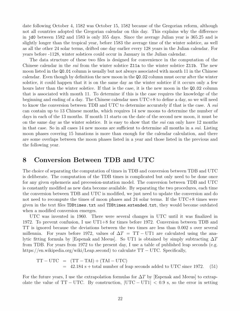
The two plots show that the motion of the Sun is more complicated than a slightly eccentricorbit, indicating that gravity from other solar system objects also has significant contribution tothe Sun’s motion. Figure 3 shows the speed of the Sun with respect to the SSB. The data indicatethat the speed is less than 16.5 m/s with the root mean square value of 12.8 m/s. As a result, thelight-time correction shifts the Sun’s position by an amount v/c < 5.5× 10−8 rad = 0.01′′.

Section 5 also mentions that the radial velocity of the Sun is about 0.5 km/s. This is mainlycaused by the eccentricity of Earth’s orbit. The value is estimated by the equation |vr| ∼ vorbe,where vorb ≈ 30 km/s is Earth’s orbital speed and e = 0.0167 is Earth’s orbital eccentricity. Thisrough equation can be derived as follows. The radial distance r of a Keplerian orbit is given bythe equation

r =a(1− e2)

1 + e cos θ, (53)

where a is the orbital semi-major axis and θ is the true anomaly. Differentiating the above equationwith respect to time gives

vr = r = − er sin θθ

1 + e cos θ= − eh sin θ

r(1 + e cos θ)= − eh sin θ

a(1− e2), (54)

where h = r2θ is the specific angular momentum. From the Newtonian two-body dynamics, wehave the following equations:

p = a(1− e2) =h2

GM, P 2 =

4π2a3

GM, (55)

where p is called the semi-latus rectum, G is Newton’s gravitational constant, M is the total massof the two-body system and P is the orbital period. The right equation is also known as Kepler’s

third law (Newtonian version). From the left equation, we can write h =√GMa(1− e2) and

equation (54) becomes

vr = −e√

GM

a(1− e2)sin θ = −2πa

P

e sin θ√1− e2

= −evorb sin θ√1− e2

, (56)

where vorb = 2πa/P is the average orbital speed. Hence, for small eccentricity, |vr| ∼ evorb.Figure 4 shows the radial velocity of the Sun relative to Earth from 2010 to 2020 calculated

using DE431. We see the expected sinusoidal-like variation from the sin θ term. Note that θis nearly but not exactly a linear function of time because of Earth’s small eccentricity4. Themaximum value of |vr| is 0.515 km/s, very close to the rough estimate.

4The true anomaly θ(t) can be calculated using the standard procedure in celestial mechanics. First calculate

25

B Radial Velocity of the Moon

Section 5 mentions that the magnitude of the Moon’s radial velocity is |vr| ∼ 0.05 km/s. It isestimated again using the rough equation |vr| ∼ evorb with vorb ≈ 2πa/P ≈ 1 km/s and e ≈ 0.05 forMoon’s orbital parameters. Figure 5 shows the radial velocity of the Moon calculated using DE431.We see that the radial velocity pattern is more complicated than that of the Sun. The maximumvalue of |vr| is 0.074 km/s, which also deviates substantially from the estimated value. Theseare caused by the perturbations of Moon’s orbit by the Sun and other planets. In particular, theSun’s perturbation on Moon’s orbit is the greatest. Since the Earth-Moon barycenter is orbitingthe Sun, the Sun’s perturbation on Moon’s orbit arises from the tidal gravity, i.e. the differencebetween Sun’s gravity on the Moon and gravity on the Earth-Moon barycenter. The Sun’s tidalgravity on the Moon is about 0.6% of Earth’s gravity on the Moon. As the Moon orbits the Earth,it experiences variation of the Sun’s tidal gravity as its position relative to the Sun changes, whichcauses periodic variation of the Moon’s orbital parameters. In other words, the Moon’s orbitalsemi-major axis, eccentricity and so on are varying with time.

We can visualize the change in Moon’s orbital parameters by plotting them versus time. BeforeI do that, it is useful to understand how the orbital parameters are determined if an object is notmoving in a strict Keplerian orbit. The usual approach is to calculate the osculating orbitalelements, which are Keplerian orbital parameters that give the position and velocity of the objectat the given time. The term “osculate” refers to a curve touching (or “kissing”) another curvewith the same tangent at the point of contact. The idea is simple. According to the two-bodyproblem of Newtonian mechanics, the relative position and relative velocity of two gravitatingbodies are determined by 6 orbital elements (a, e, i, ω,Ω, T0). Here a is the semi-major axis, e iseccentricity, i is the orbital inclination, ω is the argument of periapsis, Ω is the longitude of theascending node, and T0 is the time of periapsis passage. The angles i, ω and Ω are three Eulerangles specifying the orientation of the orbit with respect to a reference frame; a and e determinethe size and shape of the orbit; T0 specifies a time when the two bodies are closest to each other.Clearly, T0 is not unique. We can add integer multiples of orbital period P to the values of T0.

Here P is given by Kepler’s third law P = 2π√a3/(GM).

Given these 6 orbital elements, one can calculate the relative position and velocity of the twobodies moving in a Keplerian orbit at any given time. Conversely, knowing the relative positionand velocity of the two bodies at a given time, it can be shown that the 5 orbital elements a,e, i, ω and Ω can be determined uniquely provided that e 6= 0, i 6= 0 and the total mass ofthe system is known. The element T0 is determined up to an integer multiples of P . If the twobodies are moving in a strict Keplerian orbit specified by the Newtonian dynamics, the 6 orbitalelements determined by the inverse process are time independent (with the exception of T0, whichis determined up to an integer multiples of P ) provided that the coordinate axes of the referenceframe from which i, ω and Ω are measured is fixed with respect to the system’s barycenter. In thepresence of perturbation, one can still use the same equations to calculate the 6 orbital elementsfrom the relative position and velocity, but these orbital elements will change with time. These

the mean anomaly M(t) = 2π(t − T0)/P , where T0 is the time of perihelion passage and P is the orbital period.Next the eccentric anomaly E is determined by solving the Kepler equation E − e sinE = M . Then the trueanomaly is calculated by the equation tan(θ/2) =

√(1 + e)/(1− e) tan(E/2). Note that the mean anomaly M(t)

is a linear function of t, but E(t) and θ(t) are not. Another way to look at it is that the Earth moves with differentspeeds around the Sun because of its orbital eccentricity. When the Earth is closer to the Sun, it moves faster andso θ increases with a faster rate. When the Earth is farther away from the Sun, it moves slower and so θ increaseswith a slower rate. As a result, θ is not a linear function of time.

26

are the osculating orbital elements. They represent the Keplerian orbit the system would followif the perturbation were suddenly turned off at the calculation time.

Given the Moon’s geocentric position X and velocity V at a given time, the osculating semi-major axis a and eccentricity e are very easy to calculate. From the two-body Newtonian dynamics,we have the following equations.

ε = −GM2a

=1

2V 2 − GM

R⇒ a =

(2

R− V 2

GM

)−1

, (57)

where ε is the specific total orbital energy (total orbital energy per mass) of the system, R = |X|and V = |V |. This equation can also be obtained directly from the vis-viva equation in celestial me-chanics. For the Earth-Moon system, GM = GME+GMM = 8.997011390199871×10−10 AU3/day2

using the mass parameters given in Table 8 of [Folkner et al 2014]. The eccentricity is calculatedusing the equation

e =

√√√√1 +εh2

(GM)2, (58)

where the specific total orbital energy ε and specific angular momentum h are calcualted usingthe equations

ε =1

2V 2 − GM

R, h2 = |X × V |2 = R2V 2 − (X · V )2. (59)

Figures 6 and 7 show the Moon’s osculating semi-major axis and eccentricity calculated usingdata from DE431. Data show that there is only a 2% variation in the semi-major axis from theyears 1600 to 3500, but the variation in eccentricity is much larger. The eccentricity varies from0.0256 to 0.0775 with an average of 0.056. There is a factor of 3 between the maximum andminimum value! This explains why my estimate of maximum |vr| is off by a factor of 1.5. Ofcourse, this does not affect the conclusion in Section 5: dropping the factor 1/(1 + vr/c) in thecalculation of Xapparent introduces a negligible error in the computation of λM .

27

Figure 1: Trajectory of the Sun from 1950 to 2050 in the ecliptic plane of J2000.0. The plus (+)symbol at the center indicates the position of the solar system barycenter (SSB). The numbersindicate the years. The solar radius is R = 6.957 × 105 km. The Sun’s position is calculatedusing JPL’s DE431 ephemeris.

28

Figure 2: Vertical position of the Sun from the ecliptic of J2000.0. The variable Year is calculatedaccording to Year = 2000 + (JD− 2451544.5)/365.25, where JD is TDB expressed in Julian datenumber.

Figure 3: Speed of the Sun with respect to the solar system barycenter.

29

Figure 4: Radial velocity of the Sun relative to Earth from 2010 to 2020.

Figure 5: Radial velocity of the Moon relative to Earth from 2018 to 2020.

30

Figure 6: Orbital semi-major axis of the Moon from 2018 to 2020. Earth’s radius is R⊕ = 6371 km.

Figure 7: Orbital eccentricity of the Moon from 2018 to 2020.

31