Embed Size (px)
Citation preview
Stephan Sturm
Calculation of the Greeks by Malliavin Calculus
Diplomarbeit zur Erlangung des Akademischen Grades”Magister der Naturwissenschaften”
Betreuer: Walter SchachermayerInstitut fur Matematik
Universitat Wien
Februar 2004

Mudigkeit spurte er keine,nur war es ihm manchmal unangenehm,dass er nicht auf dem Kopf gehn konnte.
Georg Buchner, Lenz
Preface
It would not be correct to describe the work on this thesis, now having it fin-ished successfully, as a short and easy task. On the contrary, it took me along time and in the couse of the work I had a lot of doubts about my ownmathematical abilities. It was my old friend Josef Teichmann who proposedme to write a diploma thesis on Malliavin Calculus under his guidance. It wasfor me quite a hard, but also very joyful path starting out as a student whithhardly any knowledge in probability theory to the heights of stochastic analysis.
The goal of my diploma thesis was a profound understanding of the calcu-lation of the Greeks by Malliavin calculus in the n-dimensional, elliptic case asfirst presented by Fournie e.a. (1998) and a generalization to hypoellipticity;this generalization is the focus of current research, see e.g. the works of Malli-avin and Thalmaier (2003, preprint), Gobet and Munos (2002, preprint) andTeichmann and Touzi (working paper).
Malliavin calculus, i.e. the stochastic calculus of variations which is build upon the notion of a weak derivative on the Wiener space, the Malliavin derivative,lies in the core of the intersection of stochastic analysis, functional analysis anddifferential geometry. It is the perfect tool for a calculation of the sensitivityof the price of an option with respect to small changes in the parameters, i.e.the Greeks. The abstract notions of functional analysis allow us to write theGreeks as the expectation of the product of the original payoff function witha specific factor, the Malliavin weight which is in fact a Skorohod integral, theadjoint operator of the Malliavin derivative and a generalization of the notionof the Ito integral.
After a short introduction to martingale theory I will give the foundations ofstochastic analysis, introduce the Ito and the Stratonovich notion of the stochas-tic integral (with respect to a Brownian motion, but also in the more generalcontinuous semimartingale case) and present the classical Girsanov theory oftransformations of the probability measure. The proof of the unique existenceof the solution of a stochastic differential equation follows an introduction to itsfirst derivative with respect to the initial value, the first variation process.
The introduction of the Wiener chaos decomposition allows me to under-stand multiple Wiener-Ito integrals as iterated (classical) Ito integrals and henceto look at stochastic integration as a process of climbing up the Wiener chaos.The Malliavin derivative is introduced as the inverse climbing down and I willprove its (functional) analytic properties up to the Clark-Haussmann-Ocone for-
2
Stephan Sturm: Calculation of the Greeks by Malliavin Calculus 3
mula, in the core the chain rule. The divergence operator (or Skorohod integral)is introduced as its adjoint operator and it is shown that it coincides for pro-gressively measurable processes with the Ito integral. As last theoretical pointI will show the connection between the first variation process and the Malliavinderivative which leads us to some closing remarks on the existence and smooth-ness of densities of random variables.
The hitherto developed mathematical theory is used to answer a specificquestion of mathematical finance: What is the behavior of an option if we varythe parameters a little bit? In the jargon of finance this means to calculate theGreeks. The idea behind the notion of ”calculating” is here to develop a formulawhich is better fitted for a numerical evaluation than the simple difference quo-tient. The method is to express the derivative of the expectation as expectationof a product of the original payoff function and some weight.
For the n-dimensional elliptic case we follow the already classical paper byFournie e.a. to show that we can calculate the derivatives with respect to theinterest rate by classical Girsanov theory while for those with respect to theinitial value and the volatility the Malliavin calculus is of great use. So we canwrite the weights as Skorohod integral whose integrands depend only on theunderlying processes.
Dropping the ellipticity condition we will then show in an hypoelliptic settingwith d Brownian motions for an n-dimensional process that we can calculate theGreeks also here.
As one concrete application of this method we calculate the Greeks in theBlack-Scholes model and show the strength of the hypoelliptic formula by usingit for an approximation of the Hobson-Rogers delta. In particular the obtainedformulas allow simple numerical algorithms to approximate the solutions ofhypoelliptic partial differential equations. This feature is applied in Hubalek,Teichmann, Tompkins (2004) to fit parameters of a model to real market datawithout using sophisticated PDE techniques.
The main sources for me were the book of Revuz and Yor [RY 91] for martin-gale theory and stochastic integration with respect to continuous semimartin-gales, the manuscripts of Teichmann [Tei 02] and [Tei 03] for stochastic integra-tion, the theory of SDEs, Wiener Chaos and Malliavin Calculus, Bass [Ba 98]for the first variation process and Nualart’s book on Malliavin Calculus [Nua95]. General reference was Kallenberg [Kal 02], the calculation of the Greeks inthe elliptic setting is due to Fournie e.a. [FLLLT 99], the hypoelliptic treatmentwas inspired by Teichmann and Touzi [TT].
First of all I have to thank Josef Teichmann who initiated me to this subjectand was always there if I had to discuss some problems of my work. Sebas-tian Markt made some linguistical suggestion and thus helped me to master myproblems with the English language. All possible faults obviously remain in myresponsibility.
The Department of Financial and Actuarial Mathematics at the Technical

Stephan Sturm: Calculation of the Greeks by Malliavin Calculus 4
University of Vienna under the direction of Walter Schachermayer gave me anideal environment for my work in a very pleasant atmosphere. I am also verygrateful that the department gave my the possibility to participate in the “BerlinWorkshop on Mathematical Finance for Young Researchers”. Thanks also toCIMPA and Prof. S.G. Dani who gave me the possibility to spend two intensiveweeks at the Summer School “Probability Measures on Groups” at the TataInstitute for Fundamental Research (TIFR), Bombay.
Last but not least I have to thank all those people who spent their days andnights with me, laughing and discussing, cooking, eating (and sometimes toomuch) drinking, on the mountains, in cafes or in our flats, shortly: my friends.In particular I want to mention Herwig Czech, Ulrike Girardi, Florian Huber,Sebastian Markt, Martina Punz, Christian Selinger, Martin, Susanne and Wil-helm Sturm, Josef Teichmann and Florian Wenninger.
I want to dedicate this work to three people who always looked on my for-mation and on my studies, but sadly could not see the fruits of all their care,love and help: My aunt Anna Kopecny (1914-2001) and my grandparents MariaSturm (1920-2003) and Eduard Sturm (1920-2000).
Chapter 1
Preliminaries
Modern probability theory was founded by Andrei Nikolaevich Kolmogorovwho, claiming that “the theory of probability as mathematical discipline canand should be developed from axioms in exactly the same way as Geometry andAlgebra”, was the first to treat this subject from an axiomatic, measure theorybased point of view. It is here not the place to go into the measure theoreticdetails of the foundations of modern probability theory; we will refer to the lit-erature where needed. We give here only an introduction to stochastic process,in particular martingales, and a very short recapitulation of the basics of thetheory of tensors on Hilbert spaces.
1.1 Stochastic Processes and Martingales
In this section we will give an introduction to stochastic processes, i.e. familiesof random variables, and martingales, stochastic processes which can be thoughtas “fair games”.
1.1.1 Stochastic Processes
Definition 1.1.1 (Stochastic Process)Given an index set T , a stochastic process is a family of measurable mappingsXt, t ∈ T ⊂ R≥0 ∪ ∞, from a probability space (Ω,F , P ) to a measurablespace (E ,G), the state space.
Under the path (or trajectory) of a stochastic process we understand themapping t → Xt(ω). A process is called continuous iff for almost all ω’s thepaths are continuous.
We introduce the following notions of “proximity” of stochastic processes:
Definition 1.1.2 (Modifications and Indistinguishability)Two stochastic processes Xt, Yt, t ∈ T defined on the same probability space(Ω,F , P ) are called
5
Stephan Sturm: Calculation of the Greeks by Malliavin Calculus 6
(i) modifications of each other iff for each t ∈ T we have Xt = Yt a.s.(ii) indistinguishable iff for almost all ω ∈ Ω we have Xt = Yt for all t ∈ T .
So the difference is that for a modification the null set where both processesdiffer is dependent on t, while for indistinguishability it is required to be inde-pendent of the concrete choice of t.
Theorem 1.1.3 (Conditions for Indistinguishability)Given two stochastic processes Xt, Yt, modifications of each other. If both pro-cesses have right continuous paths a.s., then they are indistinguishable.
Proof Let A, B the null sets where Xt resp. Yt are not right continuous.Further be Nt := ω : Xt(ω) 6= Yt(ω) the null set where Xt and Yt differand N :=
⋃t∈Q
Nt. N has as rational union of null sets measure zero, so has
M := A∪B∪N . For ω /∈M we can take for every t a rational sequence tn ∈ Q,tn ↓ t, so right continuity implies that Xtn = Ytn entails Xt = Yt for all ω /∈Mindependent of the choice of t.
The following definition will be of great use for integration theory:
Definition 1.1.4 (Total and Quadratic Variation)Given a stochastic process X on Rd and a partition ∆ of the interval [0, t] with0 = t0 < t1 < ... < tn = t, we consider the sums
S∆t (X) :=
n−1∑i=0
|Xti+1 −Xti |,
T∆t (X) :=
n−1∑i=0
(Xti+1 −Xti)2.
The process X is said to be of finite total variation on [0, t], iff the total variationprocess St(X) := sup
∆S∆t (X) < ∞ and it is said to be of finite quadratic vari-
ation, iff 〈X,X〉t := lim|∆n|→0
T∆nt (X) < ∞ for a refining sequence of partitions
with mesh |∆n| tending to zero.
The next notion we introduce is a very fundamental one, the filtration:
Definition 1.1.5 (Filtration)A filtration of a probability space (Ω,F , P ) is an increasing family (Ft), t ∈ T ⊂R≥0 ∪ ∞ of sub- σ-algebras of F , i.e. Fk ⊂ Fj for k ≤ j.
For the filtered space, i.e. the probability space endowed with a filtra-tion we will write (Ω,F ,Ft, P ). By a monotone class argument there existsa F∞ :=
⋃tFt ⊂ F . Iff F∞ = F we say that the filtration converges.
Stephan Sturm: Calculation of the Greeks by Malliavin Calculus 7
Definition 1.1.6 (Usual Conditions)We say that a filtration Ft, t ∈ T satisfies the usual conditions of the StrasbourgSchool (the “conditions habituels de l’Ecole Strasbourgeoise”) or shortly the usualconditions iff
(i) Ft is complete, i.e. it contains all P-null sets (meaning that for all t, iffG ⊂ F ∈ Ft and P (F ) = 0, then G ⊂ Ft).
(ii) Ft is right-continuous, i.e. Ft = Ft+ :=⋂s>t
Fs.
In the following all our filtrations - except when otherwise stated - will sat-isfy the usual conditions and converge. The connection of stochastic processesand filtrations seems obvious:
Definition 1.1.7 (Adaptedness)A process (Xt)t∈T on (Ω,F , P ) is called adapted to the filtration Ftt∈T , iffXt is Ft-measurable for every t.
Every process Xt is adapted to its natural filtration F0t := σ(Xs : s ≤ t),
the coarsest filtration wherefore it is adapted. The usual measurability notionof processes on filtered probability spaces is the following: we say that a processX is measurable, iff the map t 7→ Xt(ω) is B(R≥0) × F∞-measurable. But forintegration theory we will need yet another notion of measurability:
Definition 1.1.8 (Progressively Measurable Processes)A processes Xt, t ∈ R≥0 is called progressively measurable with respect to thefiltration Ft, iff its restriction to [0, T ]×Ω is B([0, T ])⊗Ft-measurable for everyt ≥ 0.
A progressively measurable process is obviously measurable and adapted.We can extend this notion to subsets of R≥0 × Ω: A set A ⊂ R≥0 × Ω is calledprogressively measurable, iff its indicator function 1A is progressively measur-able. Note that progressively measurable sets form a σ-algebra.
The next objects we introduce are the so-called stopping (or optional) times:
Definition 1.1.9 (Stopping Time)A stopping time τ relative to the filtration Ft is a r.v. τ : (Ω,F ,Ft, P ) → [0,∞]such that τ ≤ t := ω : τ ≤ t ∈ Ft for every t ∈ T .
For a right-continuous filtration we can formulate this differently:
Proposition 1.1.10For a right-continuous filtration Ft, τ is a Ft-stopping time, iff τ < t ∈ Ftfor every t ∈ T .
Proof Given such a τ , then by right continuity
τ ≤ t =⋂s>t
τ < s ∈⋂s>t
Fs = Ft,
Stephan Sturm: Calculation of the Greeks by Malliavin Calculus 8
and conversely for a stopping time τ
τ < t =⋃
0<s<t
τ ≤ s =
(⋂s>t
τ ≤ sc)c
∈⋂s>t
Fs = Ft.
We note that for Ft-stopping times σ, τ and a real number α > 1 the ex-pressions σ ∧ τ(:= inf(σ, τ)), σ ∨ τ(:= sup(σ, τ)), σ+ τ and ατ are Ft-stoppingtimes too. To a given stopping time τ , the expression t ∧ τ is also a stoppingtime and we will define the stopped process by Xτ := Xt∧τ .
1.1.2 Martingales
One of the most central notions of modern probability theory is the martingale:
Definition 1.1.11 (Martingale)A real-valued process Xt defined on a filtered probability space (Ω,F ,Ft, P ) iscalled a (Ft)-martingale (resp. sub- or supermartingale), iff
(i) Xt is adapted to Ft for all t ∈ T ,(ii) E(|Xt|) <∞ for every t ∈ T ,(iii) E(Xt|Fs) = Xs (resp. ≥, ≤) for s < t.
In other words, a martingale is an adapted family of r.v.s such that for anyset A ∈ Fs, s < t it holds that∫
A
XsdP =∫A
XtdP.
Given two filtrations Ft, Gt, Ft ⊂ Gt, then every Gt-martingale is also a Ft-martingale. In particular every Ft-martingale Xt is a martingale with respectto its natural filtration σ(Xs : s ≤ t) too.
A martingale is called closed (on the right), iff there exists a X∞ ∈ L1 suchthat E(X∞|Fs) = Xs.
Proposition 1.1.12 (Stopped Discrete Martingales)Given a discrete Fn-(sub-)martingale Xn, n ≥ 0 and Hn a positive boundedstochastic process with Hn ∈ Fn−1 for n ≥ 1. Then the process Y given by
Y0 := X0
Yn := Yn−1 +Hn(Xn −Xn−1)
is a (sub)martingale, and for a stopping time τ , the stopped process Xτ = Xτ∧nis a (sub-)martingale too.
Proof It is enough to show that
E(Yn+1|Fn) = E(Yn +Hn+1(Xn+1 −Xn)|Fn)= Yn +Hn+1E(Xn+1 −Xn|Fn) ≥ Yn
Stephan Sturm: Calculation of the Greeks by Malliavin Calculus 9
with equality for Xn a martingale.For the stopping we define Hn := 1n≤τ = 1− 1τ≤n−1 ∈ Fn−1 which impliesthat Yn = Xτ is a submartingale according to the first part.
Lemma 1.1.13 (Discrete Optional Sampling)Given two bounded stopping times σ ≤ τ (i.e. σ(ω) ≤ τ(ω) ≤ M < ∞ for aconstant M independent of ω) and a discrete (sub-)martingale Xn, then it holdsthat
Xσ ≤ E(Xτ |Fσ) a.s.
with equality for X a martingale.
Proof We define with respect to the previous proposition Hn := 1n≤τ −1n≤σ ∈ Fn−1, then we have on the one hand side
Yn −X0 = Xτ −Xσ
and on the other hand side
E(Yn) = E(Yn−1 +Hn(Xn −Xn−1))= E(E(Yn−1 +Hn(Xn −Xn−1)|Fn−1)) ≥ E(Yn−1) ≥ E(Y0) = E(X0)
by iteration. Together this gives
E(Xτ ) ≥ E(Xσ).
For any B ∈ Fσ we define the following stopping times σB := σ1B +M1Bc andτB := τ1B +M1Bc for which the result above reads
E(Xσ1B +XM1Bc) ≤ E(Xτ1B +XM1Bc).
Conditioning by E(·|Fs) gives
E(Xσ1B) ≤ E(E(Xτ1B |Fs)),
whenceXσ ≤ E(Xτ |Fs) a.s.
with equality for the martingale case.
As a corollary we get optional stopping: Xσ ≤ E(Xτ |Fσ). To generalizethis lemma to arbitrary stopping times and closed martingales we have yet toprove the following statement:
Lemma 1.1.14Given a closed martingale X, then the family Xσ is u.i. for an arbitrarystopping time σ (bounded or not).
Proof First we prove the lemma for stopping times bounded by a constant M .Then by Lemma 1.1.12
Xσ = E(XM |Fσ) = E(E(X∞|FM )|Fσ) = E(X∞|Fσ)
Stephan Sturm: Calculation of the Greeks by Malliavin Calculus 10
what implies for c > 0 that∫|Xσ|>c
|Xσ|dP =∫
|Xσ|>c
|X∞|dP.
But by Chebyshev’s inequality we have
P (|Xσ| > c) ≤ 1cE(|Xσ|) ≤
1cE(|X∞|)
implying that (for c→∞) P (|Xσ| > c → 0 and∫
|Xσ|>c|Xσ|dP → 0 proving
that the family Xσ is u.i.For the generalization to unbounded stopping times we define the family U :=Xσ∧M1σ≤M +X∞1σ>M for arbitrary σ, M .This family is by the first part ofthis proof uniformly integrable. Further we can write for an arbitrary stopping
Xσ = limM→∞
(Xσ∧M1σ≤M +X∞1σ>M ) .
So Xσ is an a.s. limit of elements of U, hence it is (by Lemma 1.1.13) in U , theclosure of U in L1, which is also u.i.
Theorem 1.1.15 (Doob’s Optional Sampling)Given a closed martingale X, then it holds for two arbitrary stopping timesσ ≤ τ that
Xσ = E(Xτ |Fσ) = E(X∞|Fσ) a.s.
with equality for X a martingale.
Proof For any set B ∈ Fσ we have by Lemma 1.1.13∫B∩σ≤M
XσdP =∫
B∩σ≤M
X∞dP
since B ∩ σ ≤M = B ∩ σ ≤ σ ∧M ∈ Fσ∧M and on the other hand side itobviously holds that ∫
B∩σ=∞
XσdP =∫
B∩σ=∞
X∞dP.
This implies for M →∞ that
E(Xσ|Fσ) = E(X∞|Fσ)
and henceXσ = E(X∞|Fσ) a.s.
since the family Xσ is u.i. by the previous lemma. To establish the secondpart of the result, it is enough to observe that
Xσ = E(E(X∞|Fτ )|Fσ) = E(Xτ |Fσ) a.s.
Stephan Sturm: Calculation of the Greeks by Malliavin Calculus 11
Proposition 1.1.16For a cadlag (i.e. right continuous) adapted process X the following conditionsare a.s. equivalent:
(i) X is a martingale.(ii) For any bounded stopping time τ , Xτ ∈ L1 and E(Xτ ) = E(X0).
Proof(i) ⇒ (ii) This is a clear consequence of Doob’s Optional Sampling Theorem.(ii) ⇒ (i) For s < t and an arbitrary set B ∈ Fs, the r.v. τ := t1Bc + s1B is
a stopping time and hence
E(X0) = E(Xτ ) = E(Xt1Bc) + E(Xs1B).
On the other hand side t itself is a stopping time too, so
E(X0) = E(Xt) = E(Xt1Bc) + E(Xt1B).
Subtracting these two equations and conditioning to Fs yields Xs = E(Xt|Fs)a.s.
Corollary 1.1.17Given a martingale X and a stopping time τ , the stopped process Xτ is a mar-tingale with respect to the filtration Ft.
Proof Xτ is cadlag, adapted and for a bounded stopping time σ, also σ ∧ τ isa stopping time. Since
E(Xτσ) = E(Xσ∧τ ) = E(X0) = E(Xτ
0 )
the previous proposition implies that Xτ is a martingale.
As a consequence we get the optional stopping theorem Xσ = E(Xτ |Fσ).The next lemmata will pave us the way to Doob’s maximal inequality:
Lemma 1.1.18Given a finite submartingale Xn, 0 ≤ n ≤ N , it holds for every λ > 0 that
λP
(supnXn ≥ λ
)≤ E
(Xn1
supnXn≥λ
)≤ E
(|Xn|1
supnXn≥λ
).
Proof We define a stopping time by
τn :=
infn : Xn ≥ λ ∈ FN for n : Xn ≥ λ 6= ∅N ∈ FN for n : Xn ≥ λ = ∅.
By optional sampling (Lemma 1.1.13) we get
E(XN ) ≥ E(Xτ ) = E
(Xτ1
supnXn≥λ
)
+ E
(Xτ1
supnXn<λ
)
≥ λP
(supnXn ≥ λ
)+ E
(XN1
supnXn<λ
).
Stephan Sturm: Calculation of the Greeks by Malliavin Calculus 12
since Xτ ≥ λ on
supnXn ≥ λ
and by the definition of the stopping time
(there is no infimum for the second term). A simple subtraction achieves theleft inequality, the right one is trivial.
For the rest of this work we will use X∗ as abbreviation for supn|Xn|.
Lemma 1.1.19For a finite martingale (or a finite positive submartingale) Xn, 0 ≤ n ≤ N theinequality
λpP (X∗ ≥ λ) ≤ E (|XN |p)
holds for λ > 0 and p ≥ 1; for p > 1 we have
E (|XN |p) ≤ E
(supn|Xn|p
)≤(
p
p− 1
)pE (|XN |p) .
Proof If E (|XN |p) <∞, Jensens’s inequality implies that |Xn|p (since convex)is a submartingale
E (|Xn|p|Fs) ≥ |E (Xn|Fs) |p ≥ |Xs|p
and the previous lemma entails the first inequality.For the second part we have to concentrate on the right equation since the leftone is obvious. The previous lemma for the process |Xn| gives
λP (X∗ ≥ λ) ≤ E(|XN |1X∗≥λ
)which we will use by estimating for a fixed k < 0:
E ((X∗ ∧ k)p) = E
X∗∧k∫0
pλp−1dλ
= E
k∫0
pλp−11[0,X∗]dλ
= E
k∫0
pλp−11[0,X∗]dλ
= E
k∫0
pλp−11X∗≥λdλ
=
k∫0
pλp−1P (X∗ ≥ λ)dλ
≤k∫
0
pλp−1E(|XN |1X∗≥λ
)dλ = pE
|XN |X∗∧k∫0
λp−2dλ
=
p
p− 1E(|XN |(X∗ ∧ k)p−1
).
Now applying Holder’s inequality we get
E ((X∗ ∧ k)p) ≤ p
p− 1
(E((X∗ ∧ k)p−1 p
p−1
)) p−1p
(E (|XN |p))1p
Stephan Sturm: Calculation of the Greeks by Malliavin Calculus 13
and hence
(E ((X∗ ∧ k)p))p ≤(
p
p− 1
)p (E((X∗ ∧ k)p−1 p
p−1
))p−1
E (|XN |p)
E ((X∗ ∧ k)p) ≤(
p
p− 1
)pE (|XN |p)
such that for k →∞ we get the desired result.
Until now we remained in the domain of finite (sub-)martingales, we will ex-tend this now to get a quite more general version of Doob’s maximal inequality.
Theorem 1.1.20 (Doob’s Maximal Inequality)Let (Xt)t∈T be a right-continuous martingale or a right-continuous positive sub-martingale for an index set T which is either an interval of R ∪ ∞ or acountable subset of an interval. Then it holds for p ≥ 1, λ > 0 that
λpP (X∗ ≥ λ) ≤ suptE (|Xt|p)
and for p > 1‖X∗‖p ≤
p
p− 1supt‖Xt‖p.
Proof If T is an interval we choose a countable dense subset D ⊂ T . Wecan further choose an increasing sequence of finite subsets Dn ⊂ D such that∞⋃n=0
Dn = D which enables us to use the above lemma for theDn. Since E (|Xt|p)
increases with t, we get by passing to the limit n→∞
λpP
(supt∈D
|Xt| ≥ λ
)≤ supt∈D
E (|Xt|p)
respectively
E
(supt∈D
|Xt|p)≤(
p
p− 1
)psupt∈D
E (|Xt|p) .
But since Xt is right continuous we have supt∈D
|Xt| = X∗ and get the desired
result by taking the p-th root in the second inequality.
Note that we made no assumption of completeness or right-continuity on thefiltration Ft.
Along with semimartingales which we will encounter in the context of inte-gration theory in Section 2.4, local martingales are the most important gener-alization of the notion of the martingale.
Definition 1.1.21 (Local Martingale)Given a filtered probability space with a right continuous filtration. An adaptedprocess Mt is called a local martingale, iff there exists an increasing sequenceτn ↑ ∞ of stopping times such that Mτn −M0 is a true martingale.
Stephan Sturm: Calculation of the Greeks by Malliavin Calculus 14
Proposition 1.1.22 (Localization)Given an increasing sequence of stopping times τn ↑ ∞, then the following state-ments are equivalent:
(i) M is a local martingale.(ii) Mτn is a local martingale for every n.
Proof(i)⇒ (ii) SinceM is a local martingale, there is a localizing sequence σn ↑ ∞
such that Mσn is a true martingale. This holds true as well for an arbitrarystopping time (Mσn)τ = (Mτ )σn by optional stopping. But this implies thatMτ is a local martingale with localizing sequence σn. And since τ was arbitrarilychosen it holds especially for the τn.
(ii) ⇒ (i) Given the localizing sequences for the local martingales Mτn by(σnk ) ↑ ∞ for k →∞. We may choose indices kn such that
P(σnkn
< τn ∧ n)≤ 2−n, n ≥ 0.
The Borel-Cantelli Lemma (see [Kal 02], p.56) implies that for τ ′n := σnk ∧ τn wehave τ ′n →∞ a.s. for n→∞. By defining τ ′′n := inf
m≥nτ ′m we get a sequence with
monotone limit τ ′′n ↑ ∞ a.s. for n → ∞. To conclude it is enough to remark
that the Mτ ′n are clearly true martingales and hence the Mτ ′′n =(Mτ ′n
)τ ′′nare
true martingales too, and so M is a local martingale.
Every local martingale can be chosen uniformly integrable since if τn is a lo-calizing sequence, we we can set σn := τn∧τ which implies that σn is a localizingsequence too, and Mσn = Mτn∧τ is u.i. In the same way any continuous lo-cal martingale can - by setting σn := τn∧ inft : |Mt| = n - be chosen bounded.
1.2 Tensor Products
Here is neither the space nor the place for a fundamental treatment of algebraictensor theory, here we will only give the main definitions and central theoremswhich will be needed in the following.
Definition 1.2.1 (Tensor Product)Given two vector spaces E, F over the same field K, we denote the vector spaceof bilinear forms on E × F by B(E,F ). For each pair (x, y) ∈ E × F themapping ux,y : B(E,F ) → K given by f 7→ f(x, y) is an element of B(E,F )∗,the algebraic dual of B(E,F ). Now we can see that there is a unique bilinearmapping E × F → B(E,F )∗ given by χ : (x, y) 7→ ux,y. The linear hull ofχ(E × F ) in the dual B(E,F )∗ is denoted by E ⊗ F and called the tensor (ordirect) product of E and F ; the embedding map χ : E×F → E⊗F is called thecanonical bilinear map of E × F into E ⊗ F . We will apply the same notationfor the element ux,y which we will now write as x⊗ y.
Stephan Sturm: Calculation of the Greeks by Malliavin Calculus 15
This notions can easily be expanded to n-fold tensor products on multilinearforms which also arise as compositions of tensor products on bilinear forms.These are associative, so we do not have to struggle with brackets. The mainproperties of the tensor product are the following:
Lemma 1.2.2 (Properties of the Tensor Product)(i) For λ ∈ K and xi, yi elements of the vector space E respective F the
following rules hold:λ(x⊗ y) = (λx)⊗ y = x⊗ (λy)
(x1 + x2)⊗ y = x1 ⊗ y + x2 ⊗ y and x⊗ (y1 + y2) = x⊗ y1 + x⊗ y2(ii) Every element u ∈ E ⊗ F can (not uniquely!) be represented as
u =r∑i=1
xi ⊗ yi where the minimal such r is called the rank of u.
(iii) For the tensor product and the direct sum holds the distributive law.Given vector spaces E, F , G it holds that E ⊗ (F ⊕G) = (E ⊗ F )⊕ (E ⊗G).
In the following we will be concerned only with Hilbert space tensor productsover R. The tensor product H1 ⊗ H2 of two Hilbert spaces H1 and H2 withinner product
〈h1 ⊗ h2, g1 ⊗ g2〉H1⊗H2:= 〈h1, g1〉H1
〈g1, g2〉H2
for hi, gi ∈ Hi is a Pre-Hilbert space. The closure of this Pre-Hilbert space is aHilbert space which we will denote - without creating confusion - by H1 ⊗H2
too, and call it the tensor product of H1 and H2. Furthermore given Hilbertspace bases eii≥1 of H1 and fjj≥1 of H2, the set ei⊗fji,j≥1 forms a basisof the Hilbert space H1 ⊗H2.
Looking for Hilbert spaces Hi, Gi at the bounded linear maps ϕi : Hi → Giwe define their tensor product as a mapping H1 ⊗H2 → G1 ⊗G2 by
(ϕ1 ⊗ ϕ2)(h1 ⊗ h2) := ϕ1(h1)⊗ ϕ2(h2).
Lemma 1.2.3For the tensor product of Hilbert space mappings it holds - for the Hilbert spacenorm ‖ · ‖ respectively the supremum norm for mappings - that
(i) ‖(ϕ1 ⊗ ϕ2)(h1 ⊗ h2)‖2 = ‖ϕ1(h1)‖2‖ϕ2(h2)‖2(ii) ‖ϕ1 ⊗ ϕ2‖ = ‖ϕ1‖‖ϕ2‖
For the case of Hilbert spaces Hi := L2(Ωi,Fi, µi) with σ-finite measures µiwe have the nice isometry
L2(Ω1,F1, µ1)⊗ L2(Ω2,F2, µ2) ' L2(Ω1 × Ω2,F1 ⊗F2, µ1 ⊗ µ2)
where Ω1 × Ω2 is the topological product, F1 ⊗ F2 the product σ-algebra andµ1 ⊗ µ2 the product measure.
Chapter 2
Brownian Motion andStochastic Integration
In this chapter it is our aim to develop stochastic integration. After an intro-duction to Gaussian processes we will give a primer on Brownian motion andthen go on defining the stochastic integral with respect to Brownian motion. Inthe last sections we will try to generalize the notion of the stochastic integralby defining it for so called progressively measurable processes with respect tocontinuous semimartingales.
First we will take a look at continuity properties which we can do in a quitegeneral setting. We will recall the definition of continuity in the sense of Holderand then give the fundamental theorem of Kolmogorov and Centsov which, un-der certain conditions, assures the existence of a modification which is Holdercontinuous to a given stochastic process.
Definition 2.0.4 (Holder Continuity)A function f : (S1, ρ1) → (S2, ρ2) between two complete metric spaces S1, S2
with respective metrics ρ1, ρ2is called Holder continuous with exponent α, iff
sups 6=t
ρ2(f(s), f(t))ρ1(s, t)α
: s, t ∈ S1, ρ1(s, t) <∞<∞.
It is called locally Holder continuous iff it is Holder continuous on every boundedset.
Theorem 2.0.5 (Kolmogorov-Centsov Theorem)Given a stochastic process Xt on Rd with values in a complete metric space(S, ρ) such that for some constants C, γ, ε > 0 and for all s, t ∈ Rd the followinginequality holds:
E (ρ (Xs, Xt)γ) ≤ C · |s− t|d+ε. (2.1)
Then there exists a continuous modification Xt with sample paths which are a.s.locally Holder continuous with exponent α for every α ∈ [ 0, εγ [ .
16
Stephan Sturm: Calculation of the Greeks by Malliavin Calculus 17
Proof Here we will only develop the proof for the restriction of Xt to [0, 1]d,since for a generalized cube (where every bounded set has to be enclosed) it isthe same up to a factor.
(i) First we define for positive integers m the set of points with coordinateentries which are dyadic rational numbers up to degree m:
Dm := (k1, ..., kd) · 2−m : ki ∈ 0, 1, ..., 2m, i ∈ 1, ..., d,m ≥ 0
and then by
D :=⋃m
Dm,
the set of all points with purely dyadic coordinates in the unit cube. Further-more we define
∆m := (s, t) : s, t ∈ Dm, |s− t| = 2−m,
the set of all pairs of adjoining points in Dm. Obviously we can count exactly|∆m| = d · 2md of them.Defining ξn by ξn := sup
(s,t)∈∆n
ρ(Xs, Xt) we can estimate it by the sum over all
(s, t) ∈ ∆n. This fact and the given inequality (2.1) let us conclude
E(ξγn) ≤ E
∑(s,t)∈∆n
ρ(Xs, Xt)γ
=∑
(s,t)∈∆n
E (ρ(Xs, Xt)γ)
≤∑
(s,t)∈∆n
C · |s− t|d+ε ≤ d2nd · C · 2−n(d+ε) ≤ J2−nε (2.2)
for a constant J .(ii) Abbreviating by sm := supr ∈ Dm : r ≤ s the largest element in Dm
not greater than s we can expand for s, t ∈ D, |s− t| ≤ 2−m
ρ(Xt, Xs) ≤∞∑i=m
ρ(Xti+1 , Xti
)+ ρ(Xtm , Xsm
) +∞∑i=m
ρ(Xsi+1 , Xsi
)(2.3)
where the series are actually finite sums, whence
ρ(Xt, Xs) ≤∞∑
i=m+1
ξi + ξm +∞∑
i=m+1
ξi.
(iii) Setting now for 0 ≤ α ≤ εγ
Mα := supρ(Xs, Xt)|s− t|α
: s, t ∈ D, s 6= t
we get
Mα ≤ supm≥0
sup
2−m−1<|t−s|≤2−m
ρ(Xs, Xt)|s− t|α
: s, t ∈ D, s 6= t
≤ supm≥0
2(m+1)α sup
|t−s|≤2−m
ρ(Xs, Xt) : s, t ∈ D, s 6= t
≤ supm≥0
(2 · 2(m+1)α
∞∑i=m
ξi
)≤ 2α+1
∞∑i=0
2iαξi
Stephan Sturm: Calculation of the Greeks by Malliavin Calculus 18
by (2.3).(iv)To prove that E (Mγ
α) <∞ we have to discern the two cases γ ≥ 1 andγ < 1:γ ≥ 1:
(E (Mγα))
1γ ≤
(E
((2α+1
∞∑i=0
2iαξi
)γ)) 1γ
≤ 2α+1∞∑i=0
(2iα(E (ξγi )
1γ
))≤ 2α+1
∞∑i=0
(2iα(J2−iε
) 1γ
)≤ R
∞∑i=0
(2i(α−
εγ
)<∞.
by (2.2) for a constant R.γ < 1:
(E (Mγα)) ≤
(E
((2α+1
∞∑i=0
2iαξi
)γ))≤ 2(α+1)γE
( ∞∑i=0
(2iαξγi
))
≤ 2(α+1)γ∞∑i=0
(2iαγE (ξγi )
)≤ 2(α+1)γ
∞∑i=0
(2iαγJ2−ε
)≤ 2(α+1)γJ
∞∑i=0
2i(αγ−ε) <∞.
(v) This enables us to show easily that the mapping t → Xt(ω) is a.s.uniformly continuous for α < ε
γ : We define Ωα as the subset with uniformlycontinuous sample paths of order α; it is surely in F since
Ωα =⋃n≥0
⋂s,t∈D
ρ(Xs, Xt) ≤ n|t− s|α =⋃n≥0
Mα ≤ n.
It follows that P (Ωα) = 1 since E (Mγα) < ∞ and P (Ω0) = 1 since Ω0 =⋂
0≤α< εγ
Ωα is an intersection of decreasing measurable sets.
(vi) It only remains to construct our desired modification Xt:
Xt :=
lim
s→t,s∈DXs(ω) for ω ∈ Ω0
0 for ω /∈ Ω0
By definition as limit Xt is measurable, it is a.s. uniformly Holder continuousand it is a modification of Xt. For a sequence tn → t we have for γ ≥ 1(
E(ρ(Xt, Xt
)γ)) 1γ
≤(E(ρ(Xt, Xtn
)γ)) 1γ
+ (E (ρ (Xtn , Xt)γ))
1γ
≤ 2C · |s− t|d+ε
γ
and for γ < 1 directly
E(ρ(Xt, Xt
)γ)≤ E
(ρ(Xt, Xtn
)γ)+E (ρ (Xtn , Xt)
γ) ≤ 2C · |s−t|d+ε (2.4)
since Xtn = Xtn by definition. Applying Fatou’s Lemma (see [Kal 02], p.11) onthis equation (2.4) gives as the result Xt = Xt a.s.
Stephan Sturm: Calculation of the Greeks by Malliavin Calculus 19
2.1 Gaussian Processes
Here we will give some general results on Gaussian processes which we will needfor the construction of Brownian motion or which can help to understand andappreciate this fundamental notion of stochastic analysis. We will come back tothis subject in Chapter 3 when we will give the decomposition of Wiener chaos.
Definition 2.1.1 (Gaussian Process)A real-valued stochastic process Xt, t ∈ T is called Gaussian, iff for any choice
of t1, ..., tn ∈ T and c1, ...cn ∈ R for any n ≥ 0, the r.v.n∑k=1
ckXtk is Gaussian.
A Gaussian process is called centered, iff for all t ∈ T E(Xt) = 0. Pro-cesses Xi on Ti, i ∈ I arbitrary, are called jointly Gaussian iff the combinedprocess X := Xi
t : t ∈ Ti, i ∈ I is Gaussian. Obviously this is the case if theprocesses Xi are independent and Gaussian. Note that the combined process isnot necessarily Gaussian if the sole processes are Gaussian, but not independent.
The following theorem motivates the use of Gaussian processes to constructBrownian motion and shows that they arise naturally from the independent in-crements.
Theorem 2.1.2 (Independent Increments and Gaussian Processes)Let (Xt)0≤t≤T be a continuous process on Rd with independent increments andX0 = 0 a.s. Then Xt is a Gaussian process and there exist two continuousprocess
at : [0, T ] → Rdbt : [0, T ] →Md, (bs − br) ≥ 0 for 0 ≤ r < s ≤ T
such that Xs −Xr is N(as − ar, bs − br).
Proof For given r, s ∈ [0, T ] we divide the interval [r, s] in n subintervals of equallength. Given u ∈ Rd, we denote the corresponding increments of u(Xs −Xr)by ξn1, ..., ξnn. The continuity of Xt yields that sup
j|ξnj | → 0 for n→∞ and we
can conclude by the results on Gaussian convergence (see [Kal 02], p.92ff) that
u(Xs −Xr) =n∑j=1
ξnj is a Gaussian r.v. Since the increments are independent
this implies that Xt is Gaussian. We define
at := E(Xt)bt := cov(Xt)
and getE(Xs −Xr) = E(Xs)− E(Xr) = as − ar
0 ≤ cov(Xs −Xr) = cov(Xs)− cov(Xr) = bs − br
for 0 ≤ r < s ≤ T .The continuity of Xt implies for s → r that Xs → Xr a.s.and therefore in distribution. The same holds for at and bt, so both functionsare continuous.
Stephan Sturm: Calculation of the Greeks by Malliavin Calculus 20
2.2 Brownian Motion
The term mathematical Brownian Motion traces back to the physical phe-nomenon of the same name which was first studied by the Scottish botanistRobert Brown in 1827. He suspended pollen of the flower Clarkia pulchella inwater and observed it with his microscope. What he could see was a rapid oscil-latory motion of the pollen grains. This phenomenon had already been observedby other researchers like Antonie Van Leeuwenhoek, but Brown was actually thefirst one who really studied it. With the development of modern physics, thisphenomenon became explainable: The molecules of water (as the molecules ofevery liquid or gas) are constantly in motion, colliding with each other, bouncingback and forth which sets the pollen grains in motion. Albert Einstein intro-duced the Brownian Motion into mathematical theory by analyzing the mainfeatures of the physical phenomenon, but scaling down from the discrete bounc-ing to a continuous version. He defined the mathematical Brownian motionas Gaussian process with continuous paths and independent increments. Evenfive years before Einstein, Louis Bachelier came with a different motivation tothe same process in his dissertation Theorie de la Speculation. But it was onlyNorbert Wiener who in 1923 treated this subject with full mathematical rigorby constructing the Wiener measure.
Definition 2.2.1 (Wiener Process)A Gaussian Process (Wt)t≥0 is called a Wiener Process, iff it satisfies the fol-lowing conditions:
(i) E(Wt) = 0(ii) cov(Ws,Wt) = E(WsWt) = s ∧ t for s, t ≥ 0.
Theorem 2.2.2 (Existence of the Wiener Process)To a given probability space (Ω,F , P ) and a sequence of independent identi-cally N(0,1)-distributed r.v.s (Xn)n≥1, there exists a process satisfying the abovestated conditions.
Proof The space L2(R≥0,B(R≥0), dx) of square-integrable linear functionalsdefined on the Borel-measurable sets of the non-negative part of the real lineis a Hilbert space, and so we can pick an orthonormal basis (ei)i≥1. As wehave seen above the span of the (Xn)n≥1 forms a closed subspace H1of theHilbert space L2(Ω,F , P ). So we can for any f, g ∈ L2(R≥0,B(R≥0), dx) definethe linear Hilbert space isometry η : L2(R≥0,B(R≥0), dx) → H1 ⊂ L2(Ω,F , P )requiring that it satisfies
〈η(f), η(g)〉H1= E (η(f)η(g)) =
∞∫0
f(u)g(u)du = 〈f, g〉L2(R≥0,B(R≥0),dx).
Now we can define the Wiener process by
Wt := η(1[0,t]).
Stephan Sturm: Calculation of the Greeks by Malliavin Calculus 21
By definition (the r.v. (Xn)n≥1 were given as centered) the expectation E(Wt)is zero. For the covariance we get by the Hilbert space isometry
E(WsWt) = E(η(1[0,s])η(1[0,t])
)=
∞∫0
1[0,s](u)1[0,t](u)du
=
∞∫0
1[0,s∧t](u)du = s ∧ t
as desired.
Obviously we can not hope to have something like uniqueness of the Wienerprocess. - In contrary, there exists a lot of them.
The following corollary of the Kolmogorov-Centsov theorem shows us thatthere exists a version of the Wiener process with continuous paths.
Corollary 2.2.3To every Wiener process (Wt)t≥0 on a given probability space (Ω,F , P ) thereexists a modification (Bt)t≥0 with Holder continuous paths for any exponentα < 1
2 .
Proof Since the Wiener process Wt is Gaussian, its characteristic function ise−
tu22 . Writing Wt as
Wt = Ws + (Wt −Ws), t > s
we get - using the independence of Bs and Bt−s - for the characteristic functions
e−tu22 = e−
su22 E
(eiu(Wt−Ws)
)and so
E(eiu(Wt−Ws)
)= e−
(t−s)u2
2 . (2.5)
Writing the exponential function as series, this is
E
( ∞∑n=0
inun(Wt −Ws)n
n!
)=
∞∑n=0
(−1)n (t−s)nu2n
2n
n!= (−1)n
∞∑n=0
(t− s)nu2n
2nn!
which enables us to compare the coefficients of u:
E
(i2k(Wt −Ws)2k
(2k)!
)= (−1)k
(t− s)k
2kk!,
whence
E((Wt −Ws)2k
)=
(2k)!(t− s)k
2kk!.
Setting γ = 2k and ε = k−1 the Kolmogorov-Centsov theorem states that thereexists a locally Holder continuous modification of order 0 ≤ α < k−1
2k . All these
Stephan Sturm: Calculation of the Greeks by Malliavin Calculus 22
modification are clearly modifications of each other and since they are contin-uous too, they are indistinguishable. So by k → ∞ we get that there exists amodification Bt which is locally uniformly Holder continuous for any exponentα < 1
2 .
We remark here only that there exist no locally Holder continuous modifi-cation for any α < 1
2 .
To proceed to Brownian motion we have only to add a filtration.
Definition 2.2.4 (Brownian Motion)The standard Brownian Motion is a R-valued process (Bt)t≥0, B0 = 0 on afiltered probability space (Ω,F ,Ft, P ) satisfying the following conditions:
(i) The filtration Ft satisfies the usual conditions and converges to F .(ii) The process (Bt)t≥0 is adapted to the filtration Fn.(iii) The increments Bs−Bt of the process are independent of Ft for s ≥ t.
The adjective standard refers to the variance of the process. By Theorem2.1.2 the third condition implies that Brownian motion is a Gaussian processand by Bs = Bt + (Bs −Bt), it also implies that Brownian motion is a contin-uous martingale. But we have yet to show that it exists:
Theorem 2.2.5 (Existence of Brownian Motion)A Wiener Process with its natural filtration satisfies the above stated conditions.
Proof We only have to check if a Wiener process with its natural filtrationsatisfies the conditions stated in definition 2.2.4. That the process is adaptedto its natural filtration is trivial, hence (ii) is fulfilled. The same for (iii) sincethe Wiener process has independent increments and the filtration is the naturalone. Concerning condition one, completeness and convergence of the filtrationare obvious too. It remains only to show that the filtration is right continuous,i.e. Ft = Ft+ :=
⋂s>t
Fs.
Therefore we define a σ-algebra Gt := σ(Bv − Bu : v ≥ u > t) and prove as afirst step that F = σ(Ft ∪ Gt). Clearly σ(Ft ∪ Gt) ⊂ F , but since Bv − Bt =limn→∞
Bv − Bt+ 1n
is Gt-measurable we can see that every Bv = (Bv − Bt) + Bt,
v < t is σ(Ft ∪ Gt)-measurable, whence F ⊂ σ(Ft ∪ Gt).We have to show that every A ∈ Ft+ is also Ft-measurable or, in anotherformulation, that for every A ∈ Ft ∪ Gt the conditional expectation E(1A|Ft+)is Ft-measurable. This is trivial for the case A ∈ Ft, otherwise A ∈ Gt, whichleads us to construct a so called π-system for Gt, a collection of subsets ofF closed under finite intersections generating Gt: The inverse images underBv − Bu, v ≥ u > t are already a π system generating Gt generically. Weobserve that for any t ≤ t1 < t2 < t3 < t4
σ(Bt3 −Bt1 , Bt4 −Bt2) ⊂ σ(Bt2 −Bt1 , Bt3 −Bt2 , Bt4 −Bt3)
which entails that we we can form this π-system by intersection of independentmeasurable sets. Since Ft+ is independent of every Bv −Bu, v ≥ u > t we have
Stephan Sturm: Calculation of the Greeks by Malliavin Calculus 23
for A ∈ GtE(1A|Ft+) = E(1A)
which is Ft-measurable.The conclusion follows by a monotone class argument: Monotone limits of Ft-measurable sets remain Ft-measurable and for the sets which are finite inter-sections of sets in Ft and Gt we have for A ∈ Ft, B ∈ Ft by independence
E(1A∩B |Ft+) = 1AE(1B |Ft+)
which is Ft-measurable too, and remains it for monotone limits.To recapitulate the argument: For every A ∈ F , E(1A|Ft+) is Ft-measurable,so for A ∈ Ft+ we can conclude that E(1A|Ft+) = 1A which proves the rightcontinuity of the filtration.
As in the case of the Wiener Process we cannot hope to have something likeuniqueness of the Brownian motion. It is easy to generalize the concept of Brow-nian motion: We define the d-dimensional Brownian motion as d-dimensionalvector whose entries are independent copies of Bt.
2.3 Ito Integration
Having introduced Brownian motion one could ask if it can be used as integra-tor to define integrals along the paths of Brownian motion. Since integrationtheory in the sense of Stieltjes requires the integrator to be locally of finite totalvariation we now have to look on the variation properties of Brownian motion.
Theorem 2.3.1 (Variation Properties of Brownian Motion)For a 1-dimensional Brownian motion Bt
(i) the quadratic variation process 〈B,B〉t equals a.s. t.(ii) the total variation process ST (B) is a.s. infinite for T > 0.
Proof(i) We want to show that T∆n
t (B) → t in L2 for every refining sequence ofpartitions ∆n with mesh |∆n| → 0 for n → ∞. For a concrete partition wecalculate directly
E((T∆t (B)− t
)2)= E
(n−1∑i=0
(Bti+1 −Bti
)2 − t
)2
= E
(n−1∑i=0
((Bti+1 −Bti
)2 − (ti+1 − ti)))2
= E
(n−1∑i=0
((Bti+1 −Bti
)2 − (ti+1 − ti))2)
+2E
n−1∑0=i<j
((Bti+1 −Bti
)2 − (ti+1 − ti))((
Btj+1 −Btj)2 − (tj+1 − tj)
) .
Stephan Sturm: Calculation of the Greeks by Malliavin Calculus 24
By independence of increments we get for the second term
2n−1∑
0=i<j
(E((Bti+1 −Bti
)2 − (ti+1 − ti))E((Btj+1 −Btj
)2 − (tj+1 − tj)))
which is obviously zero, so
E((T∆t (B)− t
)2)= E
(n−1∑i=0
((Bti+1 −Bti
)2 − (ti+1 − ti))2).
Now we take a N(0, 1)-distributed r.v. Z and observe that
E(Bt+δ −Bt) = 0 = E(√δZ)
E((Bt+δ −Bt)2
)= δ = E
((√δZ)2
)implying that Bt+δ −Bt and
√δZ have the same distribution and
E((
(Bt+δ −Bt)2 − δ)2)
= E((δZ2 − δ)2
)= δ2E
((Z2 − 1)2
)=: δ2C.
So
E
(((Bti+1 −Bti
)2 − (ti+1 − ti))2)
= (ti+1 − ti)2C,
whence
E((T∆t (B)− t
)2)= C
n−1∑i=0
(ti+1 − ti)2 ≤ C
n−1∑i=0
|ti+1 − ti|2 supi|ti+1 − ti| → 0
since |∆n| → 0 for n→∞ as desired.
(ii) Assuming indirectly ST (B) < ∞ for an arbitrary T > 0, then for apartition ∆n, 0 = t0 ≤ ... ≤ tn = T
n∑i=0
|Bti+1 −Bti |2 ≤ supi
(|Bti+1 −Bti |
) n∑i=0
|Bti+1 −Bti | =
= supi
(|Bti+1 −Bti |
)S∆n
T (B) ≤ supi
(|Bti+1 −Bti |
)ST (B).
But taking a sequence of partitions with mesh |∆n| = supi|ti+1 − ti| tending to
zero we have supi|Bti+1 −Bti | → 0 by continuity of Brownian motion, implying
n∑i=0
|Bti+1 − Bti |2 → 0. This contradicts the result of the first part of this the-
orem, namely thatn−1∑i=0
|Bti+1 − Bti |2 → T . So the assumption has to be false
and ST (B) = ∞ a.s.
As it is not possible to use Stieltjes integrals, we have to search for a newnotion of integral - and it helps to know that the quadratic variation is finite onevery interval [0, T ]: The idea is to define our “stochastic integral” as L2-limit
Stephan Sturm: Calculation of the Greeks by Malliavin Calculus 25
of Riemannian sums. But first we have to define our “playground”:
We denote the set of all square integrable, progressively measurable pro-cesses Λ : R≥0 × Ω → R (i.e. progressively measurable processes satisfy-
ing E(∞∫
0
ϕ(s)2ds)
=∫Ω
∞∫0
ϕ(s, ω)2dsdP (ω) < ∞) by L2 (R≥0 × Ω,Fp, dt⊗ P ),
these are the processes for which we expect a notion of stochastic integral.
For the beginning we have to look for a more convenient subspace, the spaceE of predictable step processes, i.e. processes of the form
ut =n−1∑i=0
Fi1]ti,ti+1](t)
with Fi ∈ L2(Ω,Fti , P ) and a partition 0 = t0 ≤ ... ≤ tn.
Definition 2.3.2 (Ito Integral for Predictable Step Processes)For processes ut ∈ E we define the Ito integral (or stochastic integral) withrespect to the 1-dimensional Brownian motion by
I(u) :=n−1∑i=0
Fi(Bti+1 −Bti).
To expand our definition to progressively measurable processes we have toprove the following theorem:
Theorem 2.3.3 (Approximation of Prog. Measurable Processes)The vector space E is dense in L2 (R≥0 × Ω,Fp, dt⊗ P ).
Proof We have to give an approximation of an arbitrarily chosen elementu ∈ L2 (R≥0 × Ω,Fp, dt⊗ P ). Since progressive measurability is defined bymeasurability on intervals it is sufficient to proof this for [0, 1] instead of R≥0.In a first step we approximate the progressive measurable (and square integrable- but this goes by itself, we do not have to care about integrability) process bybounded progressive measurable processes. This goes easily by cutting down,e.g. u′ := u ∧ n, n→∞.The second step is to approximate a bounded progressively measurable processu′ by a sequence of continuous, adapted processes. We postulate that for t, h ≥ 0with h→ 0
u′h(t) :=1h
t∫t−h
u′(s)ds
is such a sequence, assuming u′(s) = 0 for s < 0 to avoid problems in theneighborhood of 0. The u′h are clearly continuous and they are adapted, sincethe integral is B([0, T ])⊗Ft-measurable. It remains to prove that the sequenceconverges in the sense of L2 (R≥0 × Ω,Fp, dt⊗ P ): Since the u′h(t) are nondecreasing, Lebesgue’s theorem on differentiation asserts that
u′h(t) → u′(t)a.e.
Stephan Sturm: Calculation of the Greeks by Malliavin Calculus 26
Now we can - thanks to the boundedness of u′ - use Lebesgue’s dominatedconvergence theorem to get
1∫0
|u′h(s)(ω)− u′(s)(ω)|2ds→ 0
for h→ 0 for every ω ∈ Ω. The same argument combined with Fubini’s theoremon multiple integrals with respect to product measures asserts
E
1∫0
|u′h(s)(ω)− u′(s)(ω)|2ds
→ 0
for h→ 0 as desired.As the third and last step we have to show that every continuous, adapted pro-cess can be approximated by predictable step processes, but this can be donein a very classical way using a refining sequence of partitions.
This enables us now to define the Ito integral in a far more general setting- for progressively measurable processes.
Definition 2.3.4 (Ito Integral)The unique continuous extension
I : L2 (R≥0 × Ω,Fp, dt⊗ P ) → L2 (Ω,F , P )
of the integral for predictable step processes is called the Ito integral with respectto Brownian motion and is denoted by
∞∫0
utdBt := I(u)
.
For t ≥ 0 we can define the definite integral by
t∫0
usdBs :=
∞∫0
us1[0,t]dBs.
Theorem 2.3.5 (Ito Lemma)The mapping I : L2 (R≥0 × Ω,Fp, dt⊗ P ) → L2 (Ω,F , P ) is a well defined Pre-Hilbert space isometry; for all u, v ∈ L2 (R≥0 × Ω,Fp, dt⊗ P ) it holds that
E(I(u)I(v)) = E
∞∫0
utvtdt
with expectation zero: E(I(u)) = 0.
Stephan Sturm: Calculation of the Greeks by Malliavin Calculus 27
Proof First we prove the theorem for predictable step processes: For the ex-pectation we calculate for every u ∈ E
E(I(u)) = E
(n−1∑i=0
Fi(Bti+1 −Bti)
)=n−1∑i=0
E(FiE(Bti+1 −Bti |Fti)
)= 0
using elementary facts of the conditional expectation.The same type of argument can be used for the inner product: Having ut :=n−1∑i=0
Fi1[ri,ri+1] and vt :=n−1∑i=0
Fi1[si,si+1] it is easy to see that there has to be a
common partition 0 = t0 ≤ ... ≤ tn such one can write ut :=n−1∑i=0
Fi1[ti,ti+1] and
ut :=n−1∑i=0
Fi1[ti,ti+1], so
E(I(u)I(v)) = E
(n−1∑i=0
Fi(Bti+1 −Bti)n−1∑i=0
Gj(Btj+1 −Btj )
)
= E
(n−1∑i=0
FiGi(Bti+1 −Bti)2
)
+E
(n−1∑i=0
FiGj(Bti+1 −Bti)(Btj+1 −Btj )
)
=n−1∑i=0
E(FiGiE
((Bti+1 −Bti)
2|Fti))
+n−1∑i=0
E(FiGj(Bti+1 −Bti)E(Btj+1 −Btj |Ftj )
)= E
(n−1∑i=0
FiGi(ti+1 − ti)
)= E
∞∫0
utvtdt
since the second term is zero and in the first term
E(B2ti+1
− 2Bti+1Bti +B2ti |Fti
)= E
(B2ti+1
−B2ti
)= ti+1 − ti.
Particularly we have E(I(u)2) = E
(∞∫0
u2tdt
).
Passing to the limits gives the general result for progressively measurable pro-cesses.
Next we want to prove some important properties of this new introducedobject.
Theorem 2.3.6 (Ito Integrals as Martingales)
The stochastic process Mt :=t∫0
usdBs is for any u ∈ L2 (R≥0 × Ω,Fp, dt⊗ P )
a martingale with respect to Ft, the natural filtration of the Brownian motion.
Stephan Sturm: Calculation of the Greeks by Malliavin Calculus 28
Proof We prove the theorem in a first step for an u ∈ E given by
us :=n−1∑i=0
Fi1]ti,ti+1](s),
so for the process M we have
Mt =
∞∫0
(n−1∑i=0
Fi1]ti,ti+1](s)
)1[0,t](s)dBs =
n−1∑i=0
Fi(Bt∧ti+1 −Bt∧ti).
Since we can always refine the partition, we can assume that t is one partitioningpoint, i.e there has to exist a k ≤ n with tk = s. Then for any t ≥ s
E(Mt|Fs) = E
(n−1∑i=0
Fi(Bt∧ti+1 −Bt∧ti)|Fs
)
=n−1∑
i=0,ti+1≤t
E(Fi(Bt∧ti+1 −Bt∧ti)|Fs
)+
n−1∑i=0,ti+1>t
E(Fi(Bt∧ti+1 −Bt∧ti)|Fs
)=
k−1∑i=0
Fi(Bt∧ti+1 −Bt∧ti) = Ms
where the second term vanishes and in the first term we add only up to k − 1since tk = s.The extension to square integrable progressively measurable processes followssimply by taking L2-limits.
This theorem has a quite important corollary which asserts the existenceof a continuous modification of a stochastic integral. So when we speak aboutstochastic integrals in the following, we can always think of them as processeswith continuous paths.
Corollary 2.3.7 (Continuous Paths of the Ito Integral)
The process Mt :=t∫0
usdBs has a modification with continuous paths.
Proof For u ∈ E this is clear since Mt =n−1∑i=0
Fi(Bt∧ti+1 − Bt∧ti) is continuous
by the continuity of Brownian motion.Otherwise we take a converging Cauchy sequence un ∈ E converging to u anddenote the associated Martingales by Mn. By Doob’s maximal inequality (The-orem 1.1.20) for p = 2 it follows for the process Mn −Mm that
P
(supt≤T
|Mnt −Mm
t | ≥ ε
)≤ 1
ε2E(|Mn
t −Mmt |2
)=
1ε2E
T∫0
|un(s)− um(s)|2ds
Stephan Sturm: Calculation of the Greeks by Malliavin Calculus 29
converging to zero for n,m→∞.This allows us to find a subsequence nk, k ≥ 0, such that
P
(| supt≤T
(Mnkt −M
nk+1t
)| ≥ 1
2k
)≤ 1
2k.
Now we can conclude by a Borel-Cantelli argument that
P
(ω : sup
t≤T
(Mnkt −M
nk+1t
)(ω) ≥ 1
2k
)= 0
which implies that Mt defined as uniform limit of the continuous processes Mn
is continuous and a modification of Mt.
All we learned till now about stochastic integration was more or less generalabstract nonsense or - in the case of predictable step processes - material fora numerical approach. But how we can calculate with Ito integrals? The nexttheorem, the celebrated Ito formula, is the major tool for all analytical calcula-tions, comparable to the fundamental theorem of calculus.
Theorem 2.3.8 (Ito Formula)Given f ∈ C2
b (R), a continuous, bounded, real valued function with continuousbounded derivatives up to order 2, and a stochastic Process
Xt := X0 +
t∫0
usdBs +
t∫0
vsds
for u, v ∈ L2 (R≥0 × Ω,Fp, dt⊗ P ), then it holds that
f(Xt) = f(X0) +
t∫0
f ′(Xs)usdBs +
t∫0
f ′(Xs)vsds+12
t∫0
f ′′(Xs)u2sds.
Here it is the last term which looks strange from the viewpoint of classi-cal analysis, it distinguishes the Ito formula for stochastic integrals from thefundamental theorem of calculus. In comparison: Setting us ≡ 0, vs ≡ 1 andX0 = 0 we get the fundamental theorem, hence the Ito integral can be seen asa generalization of the classical notion of integral. The origins of the additionalterm can be seen in the proof:
Proof First we prove the theorem under the assumption that f ∈ C∞b (R) andu, v ∈ E . For the sake of simplicity we will use the notations ∆it := ti+1 − ti,∆iB := Bti+1 −Bti and ∆iX := Xti+1 −Xti .We expand
f(Xt) = F (X0)−n−1∑i=0
f(∆iX)
Stephan Sturm: Calculation of the Greeks by Malliavin Calculus 30
by Taylor’s formula up to order 2
F (Xt) = f(X0)
+n−1∑i=0
f ′(Xti)∆iX (2.6)
+12
n−1∑i=0
f ′′(Xti)(∆iX)2 (2.7)
+12
n−1∑i=0
1∫0
f ′′′(Xti + s(∆iX)(1− s)2
)ds(∆iX)3 (2.8)
and now check the convergence term by term.Since f ′ is bounded we have for (2.6), n→∞
n−1∑i=0
f ′(Xti)∆iX
=n−1∑i=0
f ′(Xti)
ti+1∫0
usdBs −ti∫
0
usdBs +
ti+1∫0
vsds−ti∫
0
vsds
=
n−1∑i=0
f ′(Xti) (uti∆iB + vti∆it) −→t∫
0
f ′(Xs)usdBs +
t∫0
f ′(Xs)vsds
in L2 along the refining sequence by definition of the respective integrals.The term (2.7) we expand to
12
n−1∑i=0
f ′′(Xti)(∆iX)2 =12
n−1∑i=0
f ′′(Xti)u2ti(∆iB)2
+n−1∑i=0
f ′′(Xti)utivti(∆it)(∆iB)
+12
n−1∑i=0
f ′′(Xti)v2ti(∆it)2. (2.9)
Since the mesh | supi
∆it| of the refining sequence tends to zero, so does |∆iB|
by continuity. Hence the last term converges in L2 to zero since vt and f ′′ arebounded and we can estimate for a constant M :
E
(12
n−1∑i=0
f ′′(Xti)v2ti(∆it)2 − 0
)2 ≤M2
n−1∑i,j=0
(∆it)2(∆jt)2 −→ 0.
Stephan Sturm: Calculation of the Greeks by Malliavin Calculus 31
By the same argument we get for the second term
E
(n−1∑i=0
f ′′(Xti)utivti(∆it)(∆iB)− 0
)2
≤ N2n−1∑i=0
(∆it)2E((∆iB)2
)+ 2
n−1∑i,j=0
utivti(∆it)utjvtj (∆jt)E ((∆iB)(∆jB))
−→ N2n−1∑i=0
(∆it)3 −→ 0
where the second term disappears by independence of the increments of the
Brownian motion and limn→∞
n−1∑i=0
E((∆iB)2
)= t. Concerning the first term (2.9),
we write (abbreviating γti := 12f
′′(Xti)u2ti) it as
n−1∑i=0
γti(∆iB)2 =n−1∑i=0
γti((∆iB)2 − (∆it)
)+n−1∑i=0
γti(∆it) (2.10)
Here the first term converges to zero since
E
(n−1∑i=0
γti((∆iB)2 − (∆it)
)− 0
)2
= E
(n−1∑i=0
γti((∆iB)2 − (∆it)
)2)
+2E
(n−1∑i=0
γtiγtj((∆iB)2 − (∆it)
) ((∆jB)2 − (∆jt)
))
≤ Kn−1∑i=0
(∆it) + 2Ln−1∑i=0
(∆it)2 −→ 0
by analogous considerations.The second term of (2.10) converges obviously
n−1∑i=0
γti(∆it) =n−1∑i=0
12f ′′(Xti)u
2ti(∆it) −→
12
t∫0
f ′′(Xs)u2sds.
The remainder (2.8) converges to zero too, since in all the cases we have (∆it)k1(∆iB)k2
with k1 + k2 = 3 as differences which asserts, byn−1∑i=0
E((∆iB)2
)→ t and mesh
| supi
∆it| tending to zero, the vanishing of each term in the series, whence of
the whole remainder.Having now checked all the terms it remains as not necessarily zero
t∫0
f ′(Xs)usdBs +
t∫0
f ′(Xs)vsds+12
t∫0
f ′′(Xs)u2sds
Stephan Sturm: Calculation of the Greeks by Malliavin Calculus 32
as desired.We yet have to generalize the result by lifting the restrictions: Given u, v ∈L2 (R≥0 × Ω,Fp, dt⊗ P ) we can choose by Theorem (2.3.3) sequences um, vm ∈E converging a.s. to (us1[0,t])s≥0 resp. (vs1[0,t])s≥0. Since um, vm, f ′ and f ′′ arebounded we can conclude by Lebesgue’s dominated convergence theorem andthe following a.s. convergences(
f ′(Xms )ums 1[0,t](s)
)s≥0
−→(f ′(Xs)us1[0,t](s)
)s≥0(
f ′(Xms )vms 1[0,t](s)
)s≥0
−→(f ′(Xs)vs1[0,t](s)
)s≥0(
f ′(Xms )(ums )21[0,t](s)
)s≥0
−→(f ′(Xs)(us)21[0,t](s)
)s≥0
that all limits exist. Dropping the smoothness restriction does not pose a prob-lem since we can approximate f ∈ C∞b (R) uniformly by a sequence fm ∈ C2
b (R).
The following notation will be of great use: Let u, v ∈ L2 (R≥0 × Ω,Fp, dt⊗ P ),instead of
Xt := X0 +
t∫0
usdBs +
t∫0
vsds
we write as shorthand the infinitesimal expression
dXt = utdBt + vtds
where we have to introduce the following calculation rules: dBt · dBt = dt,dBt · dt = dt · dBt = 0 and dt · dt = 0. For instance the Ito formula is writtenin this notation as
df(Xt) = f ′(Xt)dXt +12f ′′(Xt)(dXt)2.
It is important to notice that this is only a notation to abbreviate the somehowlengthly integral notation and has nothing to do with derivatives which werenot yet defined.
2.4 Generalizing the Ito Integral: Integrationalong Continuous Semimartingales
It is our aim in this section to generalize the Ito calculus developed in theprevious one. So first we have to ask which of the many salient features ofBrownian motion was the reason that we could integrate along it’s paths. Go-ing some pages back we will recognize that it was the martingale propertieswhich enabled us to do so, or, more precisely, the fact that Brownian motion isa continuous local martingale. There even exists a theory of stochastic integra-tion along general semimartingales but we will restrict ourselves to continuoussemimartingales as most general class of integrators.
Stephan Sturm: Calculation of the Greeks by Malliavin Calculus 33
2.4.1 Martingales and Quadratic Variation
First we have to look at the quadratic variation again:
Proposition 2.4.1 (Finite Variation Martingales)A continuous martingale Mt does not have finite total variation unless it isconstant.
Proof The proof is quite similar to the proof of Theorem 2.3.1. Without lossof generality we may assume M0 = 0. We define the stopping time σn :=inf s : Ss ≥ 0 for the total variation ST (M) on [0, T ] entailing that the stoppedmartingale Mσn is of bounded total variation which allows us to restrict our-selves to martingales with bounded variation ST (M) < K.We take a refining sequence of partitions with mesh |∆n| → 0. For a concretepartition we have by the martingale property
E(M2t ) = E
(n−1∑i=0
(M2ti+1
−M2ti)
)= E
(n−1∑i=0
(Mti+1 −Mti)2
)
≤ E
((supi|Mti+1 −Mti |
)ST (M)
)≤ KE(|∆n|) → 0
for |∆n| → 0. It follows that M0 = 0 a.s. which yields the result.
Theorem 2.4.2 (Quadratic Variation Process)Given a continuous bounded martingale M , then the quadratic variation process〈M,M〉s is the unique continuous increasing adapted process which vanishes atzero such that
M2t − 〈M,M〉t
is a martingale. In particular this implies that continuous bounded martingalesare of finite quadratic variation.
Proof(i) Uniqueness: Assume there would be two different such processes A, B.
Then A − B is a continuous martingale with finite total variation, whence byProposition 2.4.1 A−B = 0 a.s. which implies uniqueness.
(ii) Existence: The proof of the existence of such a process is not so easy:For a given t we observe the partition ∆ with 0 = t0 < t1 < ... < tn = t. Forany s < t there exists an i ∈ 0, ..., n− 1 such that ti ≤ s < ti+1, implying
E((Mti+1 −Mti)
2|Fs)
= E((Mti+1 −Ms)2|Fs
)+ (Ms −Mti)
2.
Writing now T∆s for the quadratic sum over the partition 0 = t0 < t1 < ... <
ti ≤ s we get
E((T∆t − T∆
s |Fs)
= E
n−1∑j=i+1
(Mj+1 −Mj)2 + (Mti+1 −Mti)2 − (Ms −Mti)
2|Fs
= E
((Mt −Ms)2|Fs
)= E
(M2t −M2
s |Fs)
(2.11)
Stephan Sturm: Calculation of the Greeks by Malliavin Calculus 34
(ii)(a) We have to prove that for a sequence of partitions ∆n with mesh|∆n| the sequence T∆n
t converges in L2 (independently of the choice of thepartition). So we have to show that the difference Xn
t (M) := T∆nt − T∆′n
t for∆n, ∆′
n two different sequences of partitions converges in L2 to zero or, inother words, that E
((Xn
t (M)− 0)2)
= E((Xn
t (M))2)→ 0 for n → ∞. We
note that X(M) is a martingale since by (2.11)
E(Xt(M)|Fs) = E(T∆t (M)− T∆′
t (M)|Fs)
= E((T∆t (M)− T∆
s (M))−(T∆′
t (M)− T∆′
s (M))
+(T∆s (M)− T∆′
s (M))|Fs)
= E(M2t −M2
s |Fs)− E
(M2t −M2
s |Fs)
+ E(T∆s (M)− T∆′
s (M)|Fs)
= Xs(M) (2.12)
Writing ∆∆′ for the partition generated by taking all partitioning points of ∆and ∆′ we get by considerations analogously to (2.11) for Xt
E(X2t (M)
)= E
((T∆t (M)− T∆′
t (M))2)
= E(T∆∆′
t (X(M)))
≤ E(2(T∆∆′
t (T∆t (M)) + T∆∆′
t (T∆′
t (M))))
(2.13)
since
T∆∆′
t
(T∆t (M)− T∆′
t (M))
=n−1∑k=0
((T∆k+1(M)− T∆′
k+1(M))−(T∆k (M)− T∆′
k (M)))2
=n−1∑k=0
((T∆k+1(M)− T∆
k (M))−(T∆′
k+1(M)− T∆′
k (M)))2
≤ 2
(n−1∑k=0
(T∆k+1(M)− T∆
k (M))2 − (T∆′
k+1(M)− T∆′
k (M))2)
≤ 2(T∆∆′
t (T∆t (M)) + T∆∆′
t (T∆′
t (M)))
So it remains to show that E(T∆∆′
t (T∆t (M))
)(resp. T∆′
t (M)) converges tozero for |∆n|+ |∆′
n| → 0.(ii)(b) For a partitioning point sk in ∆∆′ we denote by tl the rightmost
point of ∆ such that tl ≤ sk < sk+1 ≤ tl+1. Since we have
T∆sk+1
(M)− Tskt∆(M) =
(Msk+1 −Mtl
)2 − (Msk−Mtl)
2
= M2sk+1
−M2sk− 2Mtl
(Msk+1 −Msk
)=
(Msk+1 −Msk
) (Msk+1 +Msk
− 2Mtl
)
Stephan Sturm: Calculation of the Greeks by Malliavin Calculus 35
we can conclude that
T∆∆′
t (T∆t (M)) =
n−1∑k=0
(T∆sk+1
(M)− T∆sk
(M))2
≤(
supk|Msk+1 +Msk
− 2Mtl |2)T∆∆′
t (M).
Applying Cauchy’s inequality to this equation we get
E(T∆∆′
t (T∆t (M))
)≤(E
(supk|Msk+1 +Msk
− 2Mtl |4)) 1
2(E
((T∆∆′
t (M))2)) 1
2
where the first factor tends - by continuity of M - to zero for |∆n|+ |∆′n| → 0
and it remains only to show that the second one is bounded.(ii)(c) Since M is bounded there exists a constant C such that |M | ≤ C and
hence by (4.11)
E(T∆t (M)
)= E
(E(T∆t (M)− T∆
0 (M)|F0
))= E
(E(M2t −M2
0 |F0
))≤ 2C2.
For the square we note that we can write(T∆t (M)
)2 as
(T∆t (M)
)2=
(n−1∑k=0
(Mtk+1 −Mtk
)2)2
= 2n−1∑
0≤k<j
(Mtk+1 −Mtk
)2 (Mtj+1 −Mtj
)2 +n−1∑k=0
(Mtk+1 −Mtk
)4= 2
n−1∑0=k
(Mtk+1 −Mtk
)2 (T∆t (M)− T∆
tk+1(M)
)+n−1∑k=0
(Mtk+1 −Mtk
)4= 2
n−1∑0=k
(T∆tk+1
(M)− T∆tk
(M))2 (
T∆t (M)− T∆
tk+1(M)
)+n−1∑k=0
(Mtk+1 −Mtk
)4and since by (4.11)
E(T∆t (M)− T∆
tk+1(M)|Ftk+1
)= E
((Mt −Mtk+1
)2 |Ftk+1
)we get
E((T∆t (M)
)2)= 2
n−1∑0=k
E((T∆tk+1
(M)− T∆tk
(M))(
M2t −M2
tk+1
))+n−1∑k=0
E((Mtk+1 −Mtk
)4)≤ 2E
((supk|M2
t −M2tk+1
|2)T∆t (M)
)+ E
((supk|M2
tk+1−M2
tk|2)T∆t (M)
)≤ 2
((2C)22C2
)+ (2C)22C2 = 24C4.
So, going backward, E((T∆t (M)
)2) is bounded for any partition, so partic-
ularly E
((T∆∆′
t (M))2)
, implying that E(T∆∆′nt
(T∆nt (M)
))tends to zero
Stephan Sturm: Calculation of the Greeks by Malliavin Calculus 36
for |∆n|+ |∆′n| → 0 and so E
((Xn
t (M))2)→ 0 for n→∞ as desired.
(iii) Properties: We have now established the unique existence of the limit〈M,M〉t in L2, it remains to show that it has a modification with the requiredproperties (i.e. to be a continuous increasing adapted process which vanishes atzero such that M2
t − 〈M,M〉t is a martingale).Adaptedness and vanishing at zero is obvious for the limit process, so it is themartingale property since by passing to the limits in (4.11) we have
E(M2t − 〈M,M〉t |Fs
)= E
((M2t −M2
s
)− (〈M,M〉t − 〈M,M〉s) +
(M2s − 〈M,M〉s
)|Fs)
= M2s − 〈M,M〉s .
Since T∆nt (M)−T∆m
t (M) is a martingale by (2.12) (and it is as a step functionright continuous) we have by Bob’s maximal inequality for p = 2
E
(sups≤t
|T∆ns (M)− T∆m
s (M)|2)
≤ 4 sups≤t
E((T∆ns (M)− T∆m
s (M))2)
= 4E((
T∆nt (M)− T∆m
t (M))2)
one can choose a subsequence ∆nk such T∆nks converges a.s. uniformly on
[0, t] hence 〈M,M〉s is continuous.It is clear that 〈M,M〉t is increasing by choosing a refining sequence dense in[0, t]. So we have for any r < s ∈
⋃n ∆n the property T∆n
r (M) ≤ T∆ns (M) for
all n > n0, the smallest n such that r, s ∈ ∆n. The rest follows by continuity.
Corollary 2.4.3 (Stopped Quadratic Variation)Given an arbitrary stopping time τ , then
〈Mτ ,Mτ 〉 = 〈M,M〉τ
Proof On one hand side, since M2 − 〈M,M〉 is a martingale,(M2 − 〈M,M〉
)τ=(M2)τ − 〈M,M〉τ = (Mτ )2 − 〈M,M〉τ ,
but on the other hand side the previous theorem states that 〈Mτ ,Mτ 〉 is theunique increasing adapted process such that (Mτ )2−〈Mτ ,Mτ 〉 is a martingale.So they have to be equal,
(Mτ )2 − 〈M,M〉τ = (Mτ )2 − 〈Mτ ,Mτ 〉
and hence 〈Mτ ,Mτ 〉 = 〈M,M〉τ .
Our next goal is to generalize these notions - into two quite distinct direc-tions. On the one hand side we will show that the quadratic variation processexists for continuous local martingales too, and on the other hand side we will- by introduction of the bracket process - drop the symmetry.
Stephan Sturm: Calculation of the Greeks by Malliavin Calculus 37
Theorem 2.4.4 (Bracket Process)Let Mt, Nt two continuous local martingales, then there exists a unique contin-uous process of finite total variation vanishing at zero such that MN − 〈M,N〉is a continuous local martingale.
This process is called the bracket process of M and N or their quadraticcovariation process.
Proof Assume first that M = N , then there exist stopping times τn ↑ ∞ suchthat Mτn is a bounded martingale. By Theorem 2.3.2 there exists for each na unique continuous process 〈Mτn ,Mτn〉 such that (Mτn)2 − 〈Mτn ,Mτn〉 is amartingale. Since 〈Mτn ,Mτn〉 = 〈Mτn+k ,Mτn+k〉τn we can define the process〈M,M〉 by requiring it to be equal to 〈M,M〉τn on [0, τn]. Here it is unique (forevery n), implying global uniqueness; and since
(M2 − 〈M,M〉
)τn = (Mτn)2 −〈Mτn ,Mτn〉 is a martingale this is the sought-after process.Asymmetry we get by polarization, setting
〈M,N〉 :=14
(〈M +N,M +N〉 − 〈M −N,M −N〉) .
This is a continuous process vanishing at zero and as difference of increasingprocesses it is of finite total variation. Furthermore it is unique by the argument2.4.2(i).
For optional stopping we get as simple consequence
Corollary 2.4.5 (Stopped Bracket)For any stopping time τ
〈Mτ , Nτ 〉 = 〈M,N〉τ = 〈M,Nτ 〉
Proof The left equality is clear by polarization and the right one by observingthat
MNτ − 〈M,N〉τ = (M −Mτ )Nτ + (MτNτ − 〈M,N〉τ )
is a local martingale which has to be unique by Theorem 2.4.4.
Also the covariation process can be described as limit of a sum, taking thedifferences of evaluation points.
Proposition 2.4.6 (Covariance as Limit)For any sequence ∆n of partitions with mesh |∆n| → 0 we can write the co-
variation process as limit of sums T∆t (M) :=
n−1∑i=0
(Mti+1 −Mti
) (Nti+1 −Nti
):
limn→∞
sups≤t
|T∆ns (M)− 〈M,N〉s | = 0
Proof We only show the proof for M = N , the rest is clear by polarization.For δ, ε > 0 we can found a suitable stopping time such that Mσ is a bounded
Stephan Sturm: Calculation of the Greeks by Malliavin Calculus 38
martingale and P (σ ≤ t) ≤ δ. On [0, σ] we have T∆t (M) = T∆
t (Mσ) and〈M,M〉 = 〈Mσ,Mσ〉, so
P
(ω : sup
s≤t|T∆s (M)− 〈M,M〉s | > ε
)≤ δ + P
(ω : sup
s≤t|T∆s (Mσ)− 〈Mσ,Mσ〉s | > ε
)tending to zero for |∆n| → 0 and a sequence δn ↓ 0
Proposition 2.4.7 (Constant Martingales)The quadratic variation vanishes only iff (for every t) Mt = M0 a.s.
Proof It is obvious, that for constant M the quadratic variation vanishes, theother direction of the proposition we prove for bounded M by setting in (2.11)s = 0 and passing to the limit
0 = E (〈M,M〉t − 〈M,M〉0 |F0) = E((Mt −M0)2|F0
),
whence Mt = M0 a.s. By optional stopping and Corollary 2.4.5 this extends tocontinuous local martingales.
The class of integrators of our generalized stochastic integrals will be thatof continuous semimartingales defined as follows:
Definition 2.4.8 (Continuous Semimartingales)A stochastic process is called a continuous (Ft)-semimartingale, iff it can bedecomposed Xt = Mt + At where Mt is a continuous local (Ft)-martingale andAt is a continuous (Ft)-adapted process of locally finite total variation withA0 = 0.
We determine its variation properties:
Proposition 2.4.9 (Semimartingale Properties)Given a continuous semimartingale Xt = Mt +At, then
(i) it is of finite quadratic variation and 〈X,X〉t = 〈M,M〉t a.s.(ii) the decomposition Xt = Mt +At is a.s. unique.
Proof (i) We take a refining sequence of partitions ∆n of [0, T ] with mesh|∆n| tending to zero. For a concrete partition we have
n−1∑i=0
(Xti+1 −Xti
)2 =n−1∑i=0
(Mti+1 −Mti
)2 + 2n−1∑i=0
(Mti+1 −Mti
) (Ati+1 −Ati
)+
+n−1∑i=0
(Ati+1 −Ati
)2.
Stephan Sturm: Calculation of the Greeks by Malliavin Calculus 39
Since by
n−1∑i=0
(Mti+1 −Mti
) (Ati+1 −Ati
)≤ sup
i|Mti+1 −Mti |ST (A)
andn−1∑i=0
(Ati+1 −Ati
)2 = supi|Ati+1 −Ati |ST (A)
we get for |∆n| → 0〈X,X〉T = 〈M,M〉T a.s.
for arbitrary T .(ii) Given two different decompositions Xt = Mt + At = Nt + Bt, then
the local martingale Mt − Nt = Bt − At is of finite total variation a.s. andM0 −N0 = A0 −B0 = 0, hence by Proposition 2.4.1 Mt −Nt = 0 a.s.
Analogous to the local martingales we can define a bracket process 〈X,Y 〉tby polarization which equals 〈M,N〉t by the above proposition.
Before developing integration theory we have yet to write something aboutthe connection between martingale and integrability properties.
Definition 2.4.10 (L2 Martingales)We denote by H2 the space of L2-bounded (Ft)-martingales, i.e. martingales Msuch that
suptE(M2
t ) <∞
The subspace of L2-bounded continuous martingales will be denoted by H2
and H20 will be used as abbreviation for the subspace of H2 which consists of
martingales Mt with M0 = 0.
Proposition 2.4.11 (H2 as Hilbert Space)Defining a norm by
‖M‖H2 :=(E(M2
∞)) 1
2 = limt→∞
(E(M2
t )) 1
2 ,
the space H2 is a Hilbert space with respect to this norm and H2 and H20 are
sub(-Hilbert-)spaces.
Proof The inner product can be obtained by polarization and Doob’s inequality(Theorem 1.1.20) asserts that every Cauchy sequence in H2 converges towardan element of H2.For the second statement we have to prove that the limit of H2-martingales re-mains continuous which can be done by Doob’s inequality too: Given a sequenceMn
t n ∈ H2 converging to Mt ∈ H2, then by Doob’s maximal inequality
‖ (Mnt −Mt)
∗ ‖2 ≤ supt‖Mn
t −Mt‖2 ≤ 2‖Mnt −Mt‖H2 → 0
Stephan Sturm: Calculation of the Greeks by Malliavin Calculus 40
for n→∞ implies that there exists a subsequence Mnkt such that
supt|Mnk
t −Mt| → 0 a.s.
asserting the continuity of Mt. The same argument is true for continuous L2-bounded martingales with M0 = 0.
The next proposition states that exactly those continuous local martingalesare in H2 which have bounded quadratic variation.
Proposition 2.4.12 (Bounded Quadratic Variation)For continuous local martingales the following two conditions are equivalent:
(i) M ∈ H2.(ii) E(〈M,M〉∞) <∞ and M0 ∈ L2.
Proof(i) ⇒ (ii) The square integrability of M0 is obvious. To prove the bound-
edness of E(〈M,M〉∞) we derive from Theorem 2.4.2 the equation
E(N2t − 〈N,N〉t
)= E
(E(N2t − 〈N,N〉t |F0
))= E
(N2
0
)(2.14)
for continuous bounded martingales N . For a given localizing sequence τn ↑ ∞of M we set σn := inft : |Mt| ≤ n∧ τn to get another localizing sequence suchthat all Mσn are martingales, so by equation (2.14) it holds that
E((Mσn)2
)− E (〈M,M〉σn) = E
(M2
0
). (2.15)
Since M ∈ H2 we have by definition suptE(M2
t ) <∞ which implies that we can
pass to the limit and get
E(M2∞)− E(〈M,M〉∞) = E
(M2
0
), (2.16)
whence E(〈M,M〉∞) <∞.(ii) ⇒ (i) In the other direction (2.15) yields
E((Mσn)2
)≤ E (〈M,M〉∞) + E
(M2
0
)≤ K <∞
for a constant K. Therefore Fatou’s Lemma implies
E(M2t
)= E
(limn→∞
(Mσn)2)≤ lim inf
nE((Mσn)2
)< K
so Mt is a L2-bounded, continuous local martingale.
Corollary 2.4.13 (Bounded Quadratic Variation)For a continuous local martingale M the following two conditions are equivalent:
(i) Ms : s ≤ t is a L2-bounded martingale.(ii) M0 ∈ L2 and E(〈M,M〉t) <∞.
Proof Analogous to the previous one.
Stephan Sturm: Calculation of the Greeks by Malliavin Calculus 41
Corollary 2.4.14 (Norm Equality)
For M ∈ H20 we have ‖M‖H2 =
∥∥∥〈M,M〉12∞
∥∥∥2.
Proof By definition of the H2-norm and equation (2.16) we have, since M0 = 0,
‖M‖H2 =(E(M2∞)) 1
2 = (E (〈M,M〉∞))12 =
∥∥∥〈M,M〉12∞
∥∥∥2
.
As the last topic of this subsection we will state some estimates for Stieltjesintegrals known as the Kunita-Watanabe inequality.
Lemma 2.4.15Given two continuous local martingales M , N and two bounded measurable pro-cesses H, K. Then it holds for t <∞ that a.s.∣∣∣∣∣∣
t∫0
HsKsd 〈M,N〉s
∣∣∣∣∣∣ ≤ t∫
0
H2sd 〈M,M〉s
12 t∫
0
K2sd 〈N,N〉s
12
Remark that the integrals here are classical Stieltjes integrals since thequadratic variation process is monotone and hence the bracket - as difference ofquadratic variation processes - is of finite total variation.
Proof First we note that it is enough to prove the statement for
H = H11[t0,t1] +H21]t1,t2] + ...+Hn1]tn−1,tn]
K = K11[t0,t1] +K21]t1,t2] + ...+Kn1]tn−1,tn]
for a specific partition ∆ of [0, t] and bounded measurable r.v. Hi, Ki, since theso defined processes are dense in the measurable bounded processes. So we getthe general statement as limit for a refining sequence ∆n of partitions withmesh tending to zero.For
〈M,N〉ts := 〈M,N〉t − 〈M,N〉swe have ∣∣∣〈M,N〉ts
∣∣∣ ≤ (〈M,M〉ts) 1
2(〈N,N〉ts
) 12
a.s. (2.17)
since for a partition ∆ we can require s, t to be partitioning points. So for arefining sequence ∆n the inequality (2.17) reads as classical Cauchy inequalitywhich is preserved for n→∞. So we estimate for our specific choice of H and
Stephan Sturm: Calculation of the Greeks by Malliavin Calculus 42
K by (2.17) and Cauchy’s inequality∣∣∣∣∣∣t∫
0
HsKsd 〈M,N〉s
∣∣∣∣∣∣ ≤n−1∑i=0
|Hi+1| |Ki+1|∣∣∣〈M,N〉ti+1
ti
∣∣∣≤
n−1∑i=0
|Hi+1| |Ki+1|(〈M,M〉ti+1
ti
) 12(〈N,N〉ti+1
ti
) 12
≤
(n−1∑i=0
H2i+1 〈M,M〉ti+1
ti
) 12(n−1∑i=0
K2i+1 〈N,N〉
ti+1ti
) 12
≤
t∫0
H2sd 〈M,M〉s
12 t∫
0
K2sd 〈N,N〉s
12
.
.
Theorem 2.4.16Given two continuous local martingales M , N and two measurable processes Hs,Ks, it holds a.s. that
t∫0
|Hs| |Ks| |d 〈M,N〉s| ≤
t∫0
H2sd 〈M,M〉s
12 t∫
0
K2sd 〈N,N〉s
12
for t ≤ ∞.
Proof Sincet∫
0
|Hs| |Ks| |d 〈M,N〉s| =
∣∣∣∣∣∣t∫
0
(Hs sgn(HsKs) sgn(d 〈M,N〉s)Ksd 〈M,N〉s)
∣∣∣∣∣∣the previous lemma gives us the result for bounded H, K and t <∞. But thesetwo conditions can be dropped since the inequality is preserved under monotonelimits (this is clearly true also for Lemma 2.4.15).
Corollary 2.4.17 (Kunita-Watanabe Inequalites)Let M , N two continuous, local martingales and H, K two measurable processes,then for p, q satisfying 1
p + 1q = 1 it holds that
E
∞∫0
|Hs| |Ks| |d 〈M,N〉|s
≤
∥∥∥∥∥∥∥ ∞∫
0
H2sd 〈M,M〉s
12
∥∥∥∥∥∥∥p
∥∥∥∥∥∥∥ ∞∫
0
K2sd 〈N,N〉s
12
∥∥∥∥∥∥∥q
and
E
∣∣∣∣∣∣∞∫0
HsKsd 〈M,N〉s
∣∣∣∣∣∣ ≤
∥∥∥∥∥∥∥ ∞∫
0
H2sd 〈M,M〉s
12
∥∥∥∥∥∥∥p
∥∥∥∥∥∥∥ ∞∫
0
K2sd 〈N,N〉s
12
∥∥∥∥∥∥∥q
Stephan Sturm: Calculation of the Greeks by Malliavin Calculus 43
Proof Clearly the inequalities of the previous Theorem and Lemma 2.4.15 arepreserved if we integrate both sides over Ω. Applying Holder’s inequality on theright side yields the result.
2.4.2 Stochastic Integrals with respect toContinuous Semimartingales
Here we will introduce the stochastic integral from a far more abstract pointof view. First we have to define the class of processes which we want to integrate:
Definition 2.4.18 (Stochastic Integrable Processes)For a given continuous square integrable martingale M ∈ H2 we define the spaceL2(M) as the equivalence class (of processes on R equal up to a set of measurezero) of progressively measurable processes K such that
‖K‖2M := E
∞∫0
K2sd 〈M,M〉s
<∞.
This can be seen as the space of square integrable, progressively measurableprocesses with respect to the measure
PM (A) := E
∞∫0
1A(s, ω)d 〈M,M〉s (ω)
for a set A ∈ B(R≥0)× F . The space L2(M) is obviously a Hilbert space withrespect to the norm ‖ · ‖M . Now we can introduce the integral:
Theorem 2.4.19Let M ∈ H2, then there exists for every K ∈ L2(M) a unique element K ·M ∈H2
0 such that
〈K ·M,N〉 = K · 〈M,N〉 :=
∞∫0
Ksd 〈M,N〉s
for every N ∈ H2. Furthermore the mapping K 7→ K ·M is a Hilbert spaceisometry L2(M) → H2
0 .
Proof(i) Uniqueness is proven by assuming the existence of two martingales M ′,
M ′′ ∈ H20 with 〈M ′, N〉 = 〈M ′′, N〉 = K ·〈M,N〉. This implies 〈M ′ −M ′′, N〉 =
0 and particularly 〈M ′ −M ′′,M ′ −M ′′〉 = 0 implying by Proposition 2.4.7 thatM ′ −M ′′ = 0 a.s. and hence, by continuity, M ′ = M ′′.
(ii) First we prove the existence for M , N ∈ H20 : The Kunita-Watanabe
inequality gives for p = q = 2 and Hs ≡ 0∣∣∣∣∣∣E ∞∫
0
Ksd 〈M,N〉s
∣∣∣∣∣∣ ≤ E
∣∣∣∣∣∣∞∫0
Ksd 〈M,N〉s
∣∣∣∣∣∣ ≤ ‖N‖H2 ‖K‖M
Stephan Sturm: Calculation of the Greeks by Malliavin Calculus 44
for an arbitrary N by the definition of ‖ · ‖M and Corollary 2.4.14 for ‖ · ‖H2 .So the mapping N → E ((K · 〈M,N〉)∞) is continuous and linear implying theexistence of an element K ·M in H2
0 such that
E ((K ·M)∞N∞) = E ((K · 〈M,N〉)∞) . (2.18)
For a stopping time τ we have by properties of the conditional expectation
E ((K ·M)τ Nτ ) = E (E ((K ·M)∞ |Fτ )Nτ ) = E ((K ·M)∞Nτ )= E ((K ·M)∞Nτ
∞) = E ((K · 〈M,Nτ 〉)∞)= E ((K · 〈M,N〉τ )∞) = E ((K · 〈M,N〉)τ ) .
Since all these processes are in H20 we get
(K ·M)τ Nτ = (K · 〈M,N〉)τ a.s.
By relaxing the (starting at zero) condition for N the result is preserved sincewe can write N as N0 +C for N0 ∈ H2
0 and a constant C (the bracket 〈X,C〉 isobviously zero). Dropping the restriction for M (so that M ∈ H2 now) requiresthat we define K ·M := K · (M −M0) for this case.
(iii) We get the isometry by a norm equation; it holds that
‖K ·M‖2H2 = E ((K ·M)∞ (K ·M)∞) = E (K · 〈M, (K ·M)∞〉)= E
(K2 · 〈M,M〉∞
)= ‖K‖2M
by equation (2.18) and the respective definition of the norms.
Definition 2.4.20 (Stochastic Integral)This unique martingale K ·M is called the stochastic integral (Ito integral) ofK with respect to M and is denoted by
(K ·M)t =:
t∫0
KsdMs
So the Ito integral is a martingale vanishing at zero. We will prove someimportant properties:
Proposition 2.4.21 (Chain Rule)Given K ∈ L2(M) and H ∈ L2(K ·M), then HK ∈ L2(M) and it holds that
(HK) ·M = H · (K ·M)
Proof H ∈ L2(K ·M) implies by 〈K ·M,K ·M〉 = K2 ·M that HK ∈ L2(M).By associativity of Stieltjes integrals we have
〈(HK) ·M,N〉 = HK · 〈M,N〉 = H · (K · 〈M,N〉)= H 〈K ·M,N〉 = 〈H · (K ·M), N〉
for an arbitrary N ∈ H2, yielding by the uniqueness of Theorem 2.4.19 that(HK) ·M = H · (K ·M).
The stochastic integral also has very nice stopping properties:
Stephan Sturm: Calculation of the Greeks by Malliavin Calculus 45
Proposition 2.4.22 (Optional Stopping)For a stopping time τ it holds that
(K ·M)τ = K ·Mτ =(K1[0,τ ]
)·M
Proof We have for an arbitrary N ∈ H2
〈(K ·M)τ , N〉 = 〈K ·M,Nτ 〉 = K · 〈M,Nτ 〉(1) = K · 〈Mτ , N〉 = 〈K ·Mτ , N〉(2) = K · 〈M,N〉τ = K1[0,τ ] · 〈M,N〉 =
⟨K1[0,τ ] ·M,N
⟩which yields the desired result by uniqueness.
It is our aim to expand the notion of the stochastic integral - in a first stepto local martingales.
Definition 2.4.23For a continuous local martingale M we define the space L2
loc(M) as the space ofclasses of progressively measurable processes K for which there exists a sequenceτn ↑ ∞ of stopping times with
E
τn∫0
K2sd 〈M,M〉s
<∞
Proposition 2.4.24For any K ∈ L2
loc(M) there exists a unique local martingale K ·M with (K ·M)0 = 0 such that for any continuous local martingale N
〈K ·M,N〉 = K · 〈M,N〉
Proof First we note that we can by a localizing procedure analogous to Propo-sition 1.1.22 choose a sequence of stopping times τn ↑ ∞ such that Mτn ∈ H2
and Kτn ∈ L2(Mτn). For every n we can now define a stochastic integralX(n) := Kτn ·Mτn and by Proposition 2.4.22 we have X(n) ≡ X(n+k) on [0, τn]for any k ≥ 0. Now we define the unique process K ·M by requiring equivalencewith X(n) on [0, τn]. This process vanishes obviously at zero, it is continuousand it is a local martingale since (K ·M)τn = Kτn ·Mτn on [0, τn] by Proposition2.4.22 which yields the result. By the same proposition follows the equation fora sequence of stopping times τn ↑ ∞:
〈K ·M,N〉τn = 〈(K ·M)τn , Nτn〉=
⟨(K1[0,τn]) ·Mτn , Nτn
⟩=(K1[0,τn]
)· 〈M,N〉τn
Before introducing integrals for continuous semimartingales we yet have todefine locally bounded processes:
Stephan Sturm: Calculation of the Greeks by Malliavin Calculus 46
Definition 2.4.25 (Locally Bounded Process)A progressively measurable process K is called locally bounded iff there exists asequence of stopping times τn ↑ ∞ with associated constants cn ≥ 0 such that|Kτn | ≤ cn.
Note that locally bounded processes are on the one hand side in L2loc(M) for
every continuous local martingale M and hence stochastic integrable and on theother hand side classical Stieltjes integrable. But we have not to fear that thisclass was chosen to narrow: By setting τn := inft : |Kt| ≥ n all continuousadapted processes have to be locally bounded.
Definition 2.4.26 (Locally Bounded Processes)Given a locally bounded process K and a continuous semimartingale X = M+A,then we define the stochastic integral K ·X as
K ·X := K ·M +K ·A
where K · A is a Stieltjes integral of K with respect to A and K · M is thestochastic integral as defined in Proposition 2.4.24.
We writet∫0
KsdXs for (K · X)t and note that iff X is a locally bounded
martingale, then also K · X, and iff X is a process with finite variation, thenK ·X is too. This asserts that the decompositionK ·X := K ·M+K ·A is unique.
Corollary 2.4.27 (Properties of the Stochastic Integral)For locally bounded processes H, K a continuous semimartingale X and anarbitrary stopping time τ it holds that
(i) (HK) ·X = H · (K ·X)(ii) (K ·X)τ = K ·Xτ =
(K1[0,τ ]
)·X
Proof For continuous local martingales the proofs go through as in Proposition2.4.21. and 2.4.22, for processes of finite total variation they are trivial and thedecomposition of the integral is unique.
We note, that iff either Kt(ω) = 0 or Xt(ω) = Xa(ω) for a.e. ω and t ∈ [a, b],then (K ·X)t(ω) is constant for a.e. ω since the quadratic and total variationare zero on this interval.
2.4.3 Ito’s Formula
As for Lebesgue integrals we have a dominated convergence theorem for stochas-tic integrals too:
Theorem 2.4.28 (Dominated Convergence)Given a continuous semimartingale X and a sequence of locally bounded pro-cesses Knn≥0 converging pointwise to zero. If there exists a locally bounded
Stephan Sturm: Calculation of the Greeks by Malliavin Calculus 47
process K with |Kn| ≤ K for every n, then (Kn ·X)n≥0 converges in probabilityuniformly to zero on compact intervals, i.e. for any T ∈ R
limn→∞
supt≤T
|(Kn ·X)t| = 0.
Proof For finite total variation processes this is clear, so we have to prove thestatement only for continuous local martingales (the rest is done by a simple tri-angle inequality). By uniform integrability (Kn)τ converges to zero in L2(Xτ )for any stopping time τ of the localizing sequence of X. Hence (Kn · X)τ
converges to zero in H2 by Proposition 2.4.11 which yields the result by anargument as in Proposition 2.4.24.
This theorem enables us to establish the connection between this abstractapproach to integration and the concrete limit of Riemannian sums:
Proposition 2.4.29 (Riemannian Sums)Given a right-continuous, locally bounded process K and a refining sequence∆n of partitions 0 = t0 < t1... <n= t of [0, t] with mesh |∆n| tending to zero,then
(K ·X)t =
t∫0
KsdXs = limn→∞
n−1∑i=0
Kti
(Xti+1 −Xti
).
Proof Assume first that K is bounded, then the sums on the right hand side
are stochastic integrals of the predictable step processesn−1∑i=0
Kti1[ti,ti+1[ which
converge pointwise to K. But since they are bounded by |Kti | ≤ ‖K‖∞ we can
use the previous theorem on dominated convergence for K −n−1∑i=0
Kti1[ti,ti+1[ to
get the result. To generalize it we can - since K is required to be locally bounded- choose a localizing sequence τn ↑ ∞.
This proposition is not only for itself interesting but gives us the possibilityto now prove an integration by parts formula for continuous semimartingales(which are obviously locally bounded).
Proposition 2.4.30 (Integration by Parts)Given two continuous semimartigales X and Y , then it holds that
XtYt = X0Y0 +
t∫0
XsdYs +
t∫0
YsdXs + 〈X,Y 〉t .
Proof Given a refining sequence ∆n of partitions with mesh tending to zerowe have for a concrete sequence
n−1∑i=0
(Xti+1 −Xti
)2 =n−1∑i=0
X2ti+1
+n−1∑i=0
X2ti −
n−1∑i=0
Xti+1Xti
= X2t +X2
0 − 2n−1∑i=0
Xti
(Xti+1 −Xti
)
Stephan Sturm: Calculation of the Greeks by Malliavin Calculus 48
and in the limit
〈X,X〉t = X2t −X2
0 − 2
t∫0
XsdXs,
whence
X2t = X2
0 + 2
t∫0
XsdXs + 〈X,X〉t
From this special case for X = Y we can derive the general one by polarization.
The integration by parts formula is a major ingredient for the Ito formulawhich can be derived for X = (X1, ..., Xd) ∈ Rd where every Xi is a continuousmartingale.
Theorem 2.4.31 (Ito Formula)Let f ∈ C2
b (Rd,R) and X ∈ Rd a continuous semimartingale, then f(X) is acontinuous semimartingale and
f(Xt) = f(X0) +d∑i=1
t∫0
∂
∂xif(Xs)dXi
s +12
d∑i,j=1
t∫0
∂2
∂xi∂xjf(Xs)d
⟨Xi, Xj
⟩s.
(2.19)
Proof We will prove the formula for the one-dimensional case to avoid that toomuch ink obscures the ideas behind the proof. (But for the d-dimensional casethe proof is analogous since the coordinate processes are in C and multiplicationswith them too.) We denote the class of C2
b -functions for which the equation(2.19) holds by C. It is easy to see that it holds for constants f(X) ≡ c andthe identity f(X) = X. Next, we show that f ∈ C implies xf(x) ∈ C: By theintegration by parts formula we get
Xtf(Xt)−X0f(X0) = (X · f(X))t + (f(X) ·X)t + 〈X, f(X)〉
=
X ·
f(X0) +
·∫0
f ′(Xs)ds+12
·∫0
f ′′(Xs)d 〈X,X〉s
t
+ (f(X) ·X)t
+
⟨X, f(X0) +
·∫0
f ′(Xs)ds+12
·∫0
f ′′(Xs)d 〈X,X〉s
⟩
=
t∫0
Xsf′(Xs)ds+
12
t∫0
Xsf′′(Xs)d 〈X,X〉s
+
t∫0
f(Xs)dXs +
⟨X,
t∫0
Xsf′(Xs)ds
⟩
=
t∫0
(Xsf(Xs))′dXs +
12
t∫0
(Xsf(Xs))′′d 〈X,X〉s
Stephan Sturm: Calculation of the Greeks by Malliavin Calculus 49
since we can expand f (in C!) by the Ito formula and since in the last term theStieltjes integrals have quadratic variation zero. By iteration this implies that allpolynomials are in C. Since the polynomials form a point separating subalgebraon (non-degenerated) compacts we can use a (Stone-) Weierstraß-argument toshow that they are dense in C. Choosing intervals [−ck, ck], ck ↑ ∞ there exists asequence pn of polynomials such that lim
n→∞sup|x|≤ck
|pn(x)− f(x)| = 0. Lebesgue’s
theorem on dominated convergence (by ‖f‖∞) entails that we can integrate thep’s twice to get polynomials Pn, satisfying for n→∞
sup|x|≤ck
|Pn(x)− f(x)| → 0
sup|x|≤ck
|P ′n(x)− f ′(x)| → 0
sup|x|≤ck
|P ′′n (x)− f ′′(x)| → 0.
Let X = M +A the canonical decomposition we get by dominated convergence
t∫0
P ′n(Xs)dXs+12
t∫0
P ′′n (Xs)d 〈X,X〉s →t∫
0
f ′(Xs)dXs+12
t∫0
f ′′(Xs)d 〈X,X〉s
in probability. So all C2b -functions on intervals [−ck, ck] are in C and letting
now k → ∞ we get the desired result that the Ito formula holds for arbitraryC2b -functions on R≥0. Note that the approximation was only one in probability
which is not necessarily uniform.
As in the case of Brownian motion we will find it convenient to apply thedifferential notation, hence the Ito formula reads
df(X) =12
d∑i=1
∂
∂xif(X)dXi +
d∑i,j=1
∂2
∂xixjf(X)d
⟨Xi, Xj
⟩.
2.4.4 The Stratonovich Integral
As the last point of this section we will present another notion of stochastic inte-gral which was developed by Fisk and Stratonovich. Even a quite strong restric-tion of the integrands can not truncate two salient features of the Stratonovichintegral: It gives us a substitution rule far more simple as Ito’s and we getdeeper insight in the convergence of the Riemannian sums.
Definition 2.4.32 (Stratonovich Integral)Given two continuous semimartingales X and Y , the Stratonovich integral of Xalong Y is defined as
t∫0
Xs dYs :=
t∫0
XsdYs +12〈X,Y 〉t .
Stephan Sturm: Calculation of the Greeks by Malliavin Calculus 50
The addition of the quadratic variation (which made the use of continuoussemimartingales - also as integrands - necessary) leads to a simplification of thechange of variables formula (by requiring a higher grade of differentiability ofthe function f!).
Theorem 2.4.33 (Stratonovich Formula)Given X ∈ Rd a continuous semimartingale and f ∈ C3(Rd,R), it holds that
df(X) =d∑i=1
∂
∂xif(X) dXi
Proof For f(x) = x2 we get for instance by definition 2t∫0
Xs dXs = X2t −X2
0
which implies by polarization the integration of parts formula for Stratonovichintegrals:
XtYt = X0Y0 +
t∫0
Xs dYs +
t∫0
Ys dXs.
From Ito’s formula for f ′
f ′(Xt) = f ′(X0) +
t∫0
f ′′(Xs)dXs +12
t∫0
f ′′′(Xs)d 〈X,X〉s
we derive
〈f ′(X), N〉t =
⟨ ·∫0
f ′′(Xs)dXs, N
⟩t
= (f ′′(Xs) · 〈Xs, N〉)t
for any continuous semimartingale N since the Stieltjes integral has quadraticvariation zero. Hence
t∫0
f ′(Xs) dXs =
t∫0
f ′(Xs)dXs + 〈f ′(Xs), Xs〉
=
t∫0
f ′(Xs)dXs +12
t∫0
f ′′(Xs)d 〈X,X〉s = f(Xt)− f(X0)
by Ito’s formula.
In Proposition 2.4.29 we saw that for right continuous, locally bounded pro-cesses K the stochastic integral can be written as limit of Riemannian sumsn−1∑i=0
Kti
(Xti+1 −Xti
). Here we took the initial point of the interval to eval-
uate the function K. But was this choice a specific one or is the stochasticintegral - as the classical Riemann integral - independent of the choice of theevaluation point in the interval? We will see that the latter is not the case, since
Stephan Sturm: Calculation of the Greeks by Malliavin Calculus 51
Proposition 2.4.34 (Riemannian Sums)Given two continuous semimartingales X, Y and a refining sequence ∆n ofpartitions 0 = t0 < ... < tn = t of [0, t] with mesh |∆n| tending to zero, then
t∫0
Ys dXs = limn→∞
n−1∑i=0
Yti+1 + Yti2
(Xti+1 −Xti
).
Proof We can write the sum asn−1∑i=0
Yti+1 + Yti2
(Xti+1 −Xti
)=n−1∑i=0
(Yti +
12(Yti+1 − Yti
)) (Xti+1 −Xti
)=
n−1∑i=0
Yti(Xti+1 −Xti
)+
12
n−1∑i=0
(Yti+1 − Yti
) (Xti+1 −Xti
)where the first sum converges by Proposition 2.4.29 to the Ito integral and thesecond one by Proposition 2.4.6 to the quadratic variation which yields the re-sult by definition of the Stratonovich integral.
Hence we have seen that the integral is not independent of choice of theevaluation point. For the initial point we get the Ito integral, for the meanpoint the Stratonovich integral. By analogous considerations we can see that
we get for the final pointt∫0
XsdYs + 〈X,Y 〉t and with λ ∈ [0, 1] for a weighted
mean point λYti + (1− λ)Yti+1 the expressiont∫0
XsdYs + (1− λ) 〈X,Y 〉t . But
for an arbitrary choice (as we can do it for classical Riemann integrals wherethe evaluation point may in every interval be differently chosen!) the stochas-tic integral does not have to exist since the “quadratic variation” in the sensesup∆T∆t (Y ) may be not finite, even if our quadratic variation defined as limit of
a refining sequence of partitions exists!
2.5 Transformations of the Probability Measure
The crucial question which lies at the core of this section is the following: forwhich transformations of the Brownian motion (with respect to the probabilityspace (Ω,F , P )) exists a probability measure Q on (Ω,F) such that the trans-formed process is again a Brownian motion, this time with respect to (Ω,F , Q)?The answer to this question gives the Cameron-Martin-Girsanov theorem, butbefore this proof we have to recall the certainly most famous elementary theo-rem on measure transformations, the Radon-Nikodym theorem.
Theorem 2.5.1 (Lebesgue-Radon-Nikodym Theorem)Given a signed measure ν and a positive measure µ on (X,A), both σ-finite,then it holds that
(i) there exist unique signed measures ν1, ν2 such that
ν1⊥µ, ν2 µ, ν1 + ν2 = ν,
Stephan Sturm: Calculation of the Greeks by Malliavin Calculus 52
the Lebesgue decomposition of ν,(ii) there exists a µ-measurable function g a.s. unique, such that ν2 = gµ
(i.e. ν2(A) =∫A
gdµ for every A ∈ A), the Radon-Nikodym derivative g = dν2dµ .
Proof By the Jordan decomposition and the σ-finiteness of the measures wecan choose µ, ν finite (true) measures without loss of generality.
Uniqueness: The uniqueness of (i) is clear since ν = ν1+ν2 = λ1+λ2 impliesν1−λ1 = λ2−ν2 with (ν1−λ1)⊥µ and (λ2−ν2) µ and ν1−λ1 = λ2−ν2 ≡ 0.If ν2 = gµ = hµ, it follows on h ≥ g that
ν2(h ≥ g) =∫
h≥g
hdµ =∫
h≥g
gdµ
and hence∫
h≥g(h − g)dµ = 0. Analogously we get
∫h≤g
(h − g)dµ = 0 and
hence
ν2(h− g) =∫
(h− g)dµ =∫
h≥g
(h− g)dµ+∫
h≤g
(h− g)dµ = 0
yields the uniqueness of (ii).Existence: We define the set
F :=
f ≥ 0 :∫A
fdµ ≤ ν(A) for all A ∈ A
which is, since f ≡ 0 is therein, not empty and so there exists a supremumα := sup
t∈F
∫fdµ < ∞. We can find a monotone increasing sequence fn with∫
fndµ→ α and the limit g := limnfn lies in F since∫
A
gdµ =∫A
limnfndµ = lim
n
∫A
fndµ ≤ ν(A)
by monotone convergence. Now we define our measures ν1, ν2 by ν2 := gµ andν1 := ν − ν2. By ν2(A) =
∫g1Adµ = 0 for A with µ(A) = 0 follows ν2 µ and
it remains only to show ν1⊥µ.This is done by defining a sequence of finite measures λn := ν1− 1
nµ with Hahndecomposition Pn ∪Nn. Setting gn := g + 1
n1Pnwe have for A ⊂ Pn∫
A
gndµ =(ν2 +
1nµ
)(A) = (ν − λn)(A) ≤ ν(A)
and for A ⊂ N clearly ∫A
gndµ = ν2(A) ≤ ν(A),
hence gn ∈ F . So α ≥∫gndµ =
∫gdµ + 1
nµ(Pn) implies µ(Pn) = 0. On theother hand side
ν1(Ω \ P ) = ν1
(⋂n
Nn
)≤ ν1(Nn) ≤
1nµ(Nn) ≤
1nµ(Ω),
Stephan Sturm: Calculation of the Greeks by Malliavin Calculus 53
so ν1(Ω \ P ) = 0 implying ν1⊥µ.
That a Brownian motion with respect to a filtered probability space en-dowed with a measure P is usually not a Brownian motion with respect to thesame probability space with another probability measure Q seems to be clear.The essence of the Cameron-Martin-Girsanov theory of changes of probabilitymeasures is the following question: For which transformations does there a newprobability measure exist, absolute continuous to the original one, under whichmartingale (or even semimartingale) properties are preserved. We will showGirsanov’s theorem on the preservation of Brownian motion under translations,but first we have to prove a lemma which we will use therefore:
Lemma 2.5.2Given a probability space (Ω,F , P ) and a non-negative function f ∈ L1(Ω,F , P )with E(f) = 1, then the probability measure Q given by dQ := fdP is welldefined and for every sub-σ-algebra G ⊂ F it holds for any X ∈ L1(Ω,F , P )that
EQ (X|G) =E (fX|G)E (f |G)
Q-a.s.
Proof For any set G ∈ G we have on the one hand side∫G
EQ (X|G) fdP =∫G
EQ (X|G) dQ =∫G
XdQ
=∫G
XfdP =∫G
E(fX|G)dP
and on the other hand side∫G
EQ (X|G) fdP = E (EQ (X|G) f1G) = E (E (EQ (X|G) f1G|G))
= E (EQ (X|G) 1GE (f |G)) =∫G
EQ(X|G)E(f |G)dP.
Putting both equations together and taking into account that they hold for ar-bitrary sets G ∈ G the equality of the two rightmost terms yields the result.
Theorem 2.5.3 (Girsanov’s Theorem)Given a progressively measurable function ut ∈ L2(R≥0 × Ω,Fp, dt ⊗ P ) anddefining
ξt := e
t∫0usdBs− 1
2
t∫0u2
sds,
then the following statements are equivalent:(i) For all T ≥ 0 there exists a probability measure QT on FT which is
absolutely continuous to P |FTsuch that
Bt −
t∫0
usds
0≤t≤T
has the law of a
Brownian motion under QT on FT ,
Stephan Sturm: Calculation of the Greeks by Malliavin Calculus 54
(ii) E(ξT ) = 1,(ii’) ξt0≤t≤T is a continuous martingale.
In this case we have on FT (the natural filtration ofBt −
t∫0
usds
0≤t≤T
) the
Radon-Nikodym derivative given by
E
(dQTdP |FT
∣∣∣∣ FT) = ξT .
Proof(ii) ⇔ (ii’) That the latter statement implies the previous one is clear by
the martingale property E(ξT ) = E(ξ0) = 1, on the other hand side defin-
ing stopping times τk := inft :
t∫0
u2sds ≥ k
gives us continuous martingales
ξτkt 0≤t≤T implying that ξt0≤t≤T is a continuous local martingale. But since
E(ξT ) = 1, it is a continuous true martingale.
(ii) ⇒ (i) We want to show thatBt −
t∫0
usds
0≤t≤T
is a Brownian motion
with respect to the measure Q (yet to define), that is, in the language of thecharacteristic functions (compare proof of Corollary 2.2.3),
E
eiλ((
Bt−t∫0urdr
)−(Bs−
s∫0urdr
)) = E
eiλ(Bt−Bs−
t∫s
urdr
) = e−λ22 (t−s).
By Lemma 2.5.2 there exists a probability measure Q with dQdP = ξT and we get
by Ito’s formula (Theorem 2.3.8)
dξr = ξr
(urdBr −
12u2rdr
)+
12ξru
2rdr = ξrurdBr.
Defining Xr as the characteristic function of the increments of the shifted Brow-nian motion
Xr := eiλ
(Br−Bs−
r∫s
uvdv
)
we get
dXr = XriλdBr −Xriλurdr +12Xri
2λ2dr
= iλXrdBr − iλXrurdr −12λ2Xrdr
and for the product
d(Xrξr) = ξrdXr +Xrdξr + dXrdξr
= iλξrXrdBr − iλξrXrurdr −12λ2Xrξrdr +
+ ξrXrurdBr + iλξrXrurdr
= ξrXrurdBr + iλξrXrdBr −12λ2Xrξrdr.
Stephan Sturm: Calculation of the Greeks by Malliavin Calculus 55
So we can calculate by the concrete representation of the previous lemma fort ≥ s
EQ(Xt|Fs) =E(XtξT |Fs)E(ξT |Fs)
=E(Xtξt|Fs)
ξs
=E
(ξs +
t∫s
XrurξrdBr + iλt∫s
ξrXrdBr − λ2
2
t∫s
Xrξrdr
∣∣∣∣Fs)ξs
=E
(ξs − λ2
2
t∫s
Xrξrdr
∣∣∣∣Fs)ξs
= 1− λ2
2
t∫s
E(Xrξrdr|Fs)ξs
dr
= EQ(Xs|Fs)−λ2
2
t∫s
EQ(Xr|Fs)dr
by martingale properties and the conditional version of Fubini’s theorem. The
equation Yt = Ys + kt∫s
Yrdr is a.s. uniquely fulfilled by Yt = ekt, so we get
EQ(Xr|Fs) = e−λ22 (t−s)
as desired, the transformed process is under the changed measure a Brownianmotion.
(i) ⇒ (ii) In the other direction we have the measure QT given and set ψ :=dQT
dP |FT
∈ L1(Ω,FT , P |FT). Then for any h ∈ L2([0, T ]) the exponentials eψ(h)
are dense in L2(Ω,FT , P |FT) and L2(Ω,FT , QT ), so for non-negative bounded
functions it holds that
E
fBt − t∧τk∫
0
usds
ξτk
T
= E(f(Bt)) (2.20)
by the same methods as in the other direction and, obviously, E(ξτk
T ) = 1. Butby the definition of ψ we have
E
fBt − t∫
0
usds
ψ
= E(f(Bt)) (2.21)
too, so by conditioning (2.20) and (2.21) it follows that ξτk
T = E(ψ|Fτk
T ) a.s.which assures us that we can pass to the limit k ↑ ∞, so E(ξT ) = 1.
Since it is not always easy to show that E(ξT ) = 1 or that ξt0≤t≤T is amartingale one might be interested in an easier sufficient condition (which is,indeed, far from being necessary):
Stephan Sturm: Calculation of the Greeks by Malliavin Calculus 56
Corollary 2.5.4 (Novikov’s Condition)
If E
e 12
T∫0u2
sds
<∞, then ξt0≤t≤T is a true martingale, hence the absolute
continuous probability measure QT of Girsanov’s theorem exists.
Proof
(i) In a first step we proof that Novikov’s condition implies that e
t∫0usdBs
isan uniformly integrable submartingale: For stopping times τn as above we have
e12
T∧τn∫0
usdBs
= e12
T∧τn∫0
usdBs− 14
T∧τn∫0
u2sdse
14
T∧τn∫0
u2sds,
so the Cauchy-Schwarz inequality implies
E
e 12
T∧τn∫0
usdBs
≤ E(ξτn
T )12E
e 12
T∧τn∫0
u2sds
12
<∞
and since the limit n→∞ on the left hand side is by the choice of the stoppingtimes monotone, we can conclude that
E
e 12
T∫0usdBs
<∞.
Furthermore e12
T∫0usdBs
is an u.i. submartingale since 12
T∫0
usdBs is an u.i. mar-
tingale.(ii) For every a ∈]0, 1[ we get
e
t∫0ausdBs− 1
2
t∫0(aus)2ds
= ea2
(t∫0usdBs− 1
2
t∫0u2
sds
)ea
t∫0usdBs(1−a)
= (ξt)a2(Zat )1−a
2
for the u.i. submartingale
Zat := e
(a
1+a
t∫0usdBs
);
the family Zaτ , τ a stopping time, is u.i. by Lemma 1.3.14 which can beproven analogously for submartingales (instead of martingales). We can nowapply Holder’s inequality for 1
1a2
+ 11
1−a2= 1 to get for some Γ ∈ F and a
stopping time τ
E
1Γe
T∧τ∫0
ausdBs− 12
T∧τ∫0
(aus)2ds
≤ E (ξτt )a2
E (ZT∧τ )1−a2
= E (ZT∧τ )1−a2
Stephan Sturm: Calculation of the Greeks by Malliavin Calculus 57
since E (ξτt ) = 1. So eT∧τ∫0
ausdBs− 12
T∧τ∫0
(aus)2ds
τ
is an u.i. family and henceet∫0ausdBs− 1
2
t∫0(aus)2ds
0≤t≤T
an u.i. martingale. This implies
1 = E
eT∫0ausdBs− 1
2
T∫0(aus)2ds
≤ E
eT∫0usdBs− 1
2
T∫0u2
sds
a2
E(ZaT )1−a2
(2.22)
and since
ZaT ≤ 1
T∫0usdBs<0
+ e12
T∫0u2
sdBs
1
T∫0usdBs>0
we can use dominated convergence to conclude that
lima↑1
E(ZaT )1−a2
= 1.
So letting a ↑ 1 in (2.22) we get E(ξT ) ≥ 1 whence E(ξT ) = 1 yielding theresult, namely that ξt0≤t≤T is a true martingale.
Chapter 3
Stochastic DifferentialEquations
The subject of this chapter are stochastic differential equations (abbreviatedSDEs), surely the most important application of the notions of stochastic cal-culus. As ordinary or partial differential equations have wide use for modelingdeterministic phenomena, so stochastic differential equations can serve as a toolfor the description of stochastic phenomena, hence phenomena whose develop-ment in time is scattered by a white noise effect.
Definition 3.0.5 (Stochastc Differential Equation)A (strong) solution of a stochastic differential equation is an adapted stochasticprocess Xx
t : (Ω,F ,Ft, P ) → Rn with continuous paths and initial value Xx0 =
x ∈ Rn which satisfies for vector fields V ;V 1, ...V d ∈ Rn → Rn the equation
Xxt = x+
t∫0
V (Xxs ) ds+
d∑i=1
t∫0
V i (Xxs ) dBis
for t ≥ 0.
Following the notation of the previous chapter we will write
dXxt = V (Xx
t )dt+d∑i=1
V i(Xxt )dBit
as a short form of this SDE. In opposition to the strong solution we call a pair(Ft, Xx
t ) to a given probability space (Ω,F , P ) satisfying the above conditionsa weak solution of the SDE. The vector field V is called the (Ito)-drift and thevector fields V i the volatilities.
3.1 Some Inequalities
In this chapter we will a lot of inequalities need for the proofs. Besides thewell known Holder inequality and Doob’s inequality for continuous martingales
58
Stephan Sturm: Calculation of the Greeks by Malliavin Calculus 59
we will be concerned with Gronwall’s lemma and the Burkholder-Davis-Gundyinequalities. Gronwall’s lemma gives us an exponential restriction for functionswhich can be estimated by an integral over their past.
Lemma 3.1.1 (Gronwall’s Lemma)Let v(t) : [0, T ] → R≥0 be a bounded and non-negative measurable function suchthat
v(t) ≤ b+ a
t∫0
v(s)ds
for t ∈ [0, T ] and some a, b ≥ 0. Then it holds that
v(t) ≤ beat
for all t ∈ [0, T ].
Proof Since v(t) is bounded we can define a function by w(t) :=t∫0
v(s)ds
which is, since v(t) has non-negative values, monotone increasing. So we can,even if w(t) is not differentiable, note that
0 ≤ lim suph→0
w(t+ h)− w(t)h
≤ b+ aw(t)
and hence
w(t) ≤t∫
0
(b+ aw(s)) ds. (3.1)
Now we define f(t) := e−atw(t) for t ∈ [0, T ] and conclude by basic theoremson Stieltjes integrals and (3.1) that the following inequality holds:
f(t) =
t∫0
1df(s) =
t∫0
e−asdw(s) +
t∫0
w(s)de−as
≤t∫
0
e−as (b+ aw(s)) ds+
t∫0
w(s)(−a)e−asds
=
t∫0
be−asds =b
a
(eat − 1
)e−at
By the definition of f(t) we get w(t) ≤ ba (eat − 1) and hence by the initial
boundedness condition of v(t)
v(t) ≤ b+ aw(t) ≤ beat.
Stephan Sturm: Calculation of the Greeks by Malliavin Calculus 60
Another important tool are the Burkholder-Davis-Gundy (or abbreviatedBDG) inequalities for continuous (local) martingales which estimate the p-thmean oft the supremum process M∗ by that of the root of the quadratic varia-tion process. We prove the inequalities first in a restricted case to develop thena procedure to generalize them for arbitrary p > 0.
Lemma 3.1.2For any p ≥ 2 there exists a constant Cp such that for every continuous localmartingale M vanishing at zero the following inequality holds:
E
((sup
0≤s≤∞|Ms|
)p)= E ((M∗
∞)p) ≤ CpE(〈M,M〉
p2∞
).
Proof Remark first that it is enough to prove the lemma for bounded martin-gales M , since for a given localizing sequence τn ↑ ∞ we can define by continuitystopping times σn := inft : |Mt| = n which also form a localizing sequenceand all the respective Mσn are bounded martingales. So by passing to the limitσn ↑ ∞ we get the result.Since the function f(x) = |x|p is in C2
b (R) we can apply Ito’s formula to get fort→∞
|M∞|p =
∞∫0
p|Ms|p−1 sgn(Ms)dMs +12
∞∫0
p(p− 1)|Ms|p−2d 〈M,M〉s ,
which implies (since the expectation of stochastic integrals of processes vanishingat zero is zero) by taking the expectation
E (|M∞|p) =p(p− 1)
2E
∞∫0
|Ms|p−2d 〈M,M〉s
≤ p(p− 1)
2E((M∗
∞)p−2 〈M,M〉∞)
≤ p(p− 1)2
∥∥∥(M∗∞)p−2
∥∥∥p
p−2
‖〈M,M〉∞‖ p2
by a classical supremum estimate for Stieltjes integrals by Holder’s inequality
for(
pp−2
)−1
+(p2
)−1 = 1. But by Doob’s maximal inequality (Theorem 1.1.20)
(E (|M∗∞|p))
1p = ‖M∗
∞‖p ≤p
p− 1‖M∞‖p =
p
p− 1(E (|M∞|p))
1p ,
implying that
E ((M∗∞)p) ≤
(p
p− 1
)pE (|M∞|p)
≤(
p
p− 1
)pp(p− 1)
2
∥∥∥(M∗∞)p−2
∥∥∥p
p−2
(E(〈M,M〉
p2∞
)) 2p
≤ CpE(〈M,M〉
p2∞
)
Stephan Sturm: Calculation of the Greeks by Malliavin Calculus 61
for a constant Cp since we can assume that E(〈M,M〉
p2∞
)≥ 1 without loss
of generality (because otherwise we could could make the whole estimate for amultiple since 〈M,M〉 = 0 only if M is constant by Theorem 2.4.7).
Lemma 3.1.3For any p ≥ 4 there exists a constant cp such that for every continuous localmartingale M vanishing at zero the following inequality holds:
cpE(〈M,M〉
p2∞
)≤ E ((M∗
∞)p) .
Proof In this proof we let c1p, ... signify different constants depending onlyon p. From the integration of parts formula for continuous semimartingales(Proposition 2.4.30) we derive
M2t = 2
t∫0
MsdMs + 〈M,M〉t
implying by a triangle inequality
|〈M,M〉t| ≤
∣∣∣∣∣∣2t∫
0
MsdMs
∣∣∣∣∣∣+ ∣∣M2t
∣∣ .Under E
((·)
p2
)this gives for t→∞
E((〈M,M〉t)
p2
)≤ c1p
E∣∣∣∣∣∣
∞∫0
MsdMs
∣∣∣∣∣∣
p2+ E ((M∗
∞)p) . (3.2)
Since·∫
0
MsdMs is by definition a continuous local martingale vanishing at zero,
we can apply the previous lemma, so
E
sup0≤s≤∞
∣∣∣∣∣∣t∫
0
MsdMs
∣∣∣∣∣∣p ≤ CpE
⟨ ·∫0
MsdMs,
·∫0
MsdMs
⟩ p2
∞
implying
E
∣∣∣∣∣∣∞∫0
MsdMs
∣∣∣∣∣∣p ≤ c2pE
∞∫
0
M2s d 〈Ms,Ms〉s
p2 .
Applying this estimate on the inequality (3.2) we get
E(〈M,M〉
p2∞
)≤ c3p
E ((M∗∞)p) + E
∞∫
0
M2s d 〈M,M〉s
p4 ≤
≤ c4p
(E ((M∗
∞)p) +(E ((M∗
∞)p)E(〈M,M〉
p2∞
)) 12)
Stephan Sturm: Calculation of the Greeks by Malliavin Calculus 62
by a supremum estimate for the Stieltjes integral and equivalence of norms.Abbreviating
x =(E(〈M,M〉
p2∞
)) 12
y = (E ((M∗∞)p))
12
this readsx2 ≤ c4p(y
2 + xy)
or0 ≥ x2 − c4pxy − c4py
2.
Since the adjoint quadratic equation has by Vieta for x two real solutions oftype c5py this entails that we can choose for every p ≥ 4 a constant cp such thatthe inequality holds.
To generalize these results to all positive p’s we will use a reduction processbased on the notion of the dominated process.
Definition 3.1.4A positive, adapted right-continuous process X is said to be dominated by anincreasing (non-negative) process A, iff for every bounded stopping time τ itholds that E(Xτ ) ≤ E(Aτ ).
Lemma 3.1.5Given a process X dominated by a continuous process A, then there exist positivereal numbers x, y such that
P (ω : X∗∞ > x,A∞ ≤ y) ≤ 1
xE (A∞ ∧ y) .
Proof Defining stopping times ρ := inft : At > y and σ := inft : Xt > xwe have ω : A∞ ≤ y = ω : ρ = ∞ and - for any n ≥ 0 - ω : X∗
n > x ⊂ω : σ <∞, so we can estimate by Chebyshev’s inequality and dominance
P (ω : X∗n > x,A∞ ≤ y) ≤ P (ω : σ <∞, ρ = ∞)
≤ P (ω : Xσ∧ρ > x)
≤ 1xE (Xσ∧ρ) ≤
1xE (Aσ∧ρ) .
Since Aρ = At1inft:At>y = y by continuity of A we have Aσ∧ρ ≤ A∞ ∧ y andconclude that for an arbitrary n ≥ 0
P (ω : X∗n > x,A∞ ≤ y) ≤ 1
xE (A∞ ∧ y) .
Applying Fatou’s Lemma yields the result.
We use this result to prove the proper reducing lemma:
Stephan Sturm: Calculation of the Greeks by Malliavin Calculus 63
Lemma 3.1.6Given a stochastic process X dominated by a continuous process A, it holds forany k ∈]0, 1[ that
E((X∗
∞)k)≤ 2− k
1− kE(Ak∞
).
Proof Taking a continuous increasing function f : R≥0 → R≥0 with f(0) = 0we can reason by Fubini’s theorem
E (f(X∗∞)) = E
∞∫0
1X∗∞df(x)
≤
∞∫0
(P (ω : X∗∞ > x,A∞ ≤ x) + P (ω : A∞ > x)) df(x)
≤∞∫0
(1xE (A∞ ∧ x) + P (ω : A∞ > x)
)df(x)
≤∞∫0
(1xE(A∞1A∞≤x
)+ 2P (ω : A∞ > x)
)df(x)
= E
A∞ ∞∫A∞
1xdf(x)
+ 2E (f(A∞))
since E(A∞ ∧ x) ≤ E(A∞1A∞≤x
)+ xP (A∞ > x). Setting now f(x)xk we
get
E((X∗
∞)k)
≤ E
A∞ ∞∫A∞
1xdxk
+ 2E(Ak∞
)≤
(2 +
k
1− k
)E(Ak∞
)=
2− k
1− kE(Ak∞
)since
∞∫A∞
1xdx
k = kk−1x
k−1k
∣∣∣∞Ak∞
= k1−kA
k−1∞ .
Theorem 3.1.7 (BDG Inequalities)Given p > 0, there exist two (non-negative) universal constants cp and Cp suchthat for all continuous local martingales M vanishing at zero
cpE(〈M,M〉
p2∞
)≤ E ((M∗
∞)p) ≤ CpE(〈M,M〉
p2∞
).
Proof For the cases p ≥ 4 resp. p ≥ 2 the inequalities are already proven. Forthe right inequality we set X = (M∗)2 (which is obviously continuous, positiveand adapted) and A = C2 〈M,M〉 (clearly continuous and increasing) so thatthe above lemma gives us
E((M∗
∞)2k)≤ 2− k
1− kCk2E
(〈M,M〉k∞
),
Stephan Sturm: Calculation of the Greeks by Malliavin Calculus 64
hence filling the gap for p ∈]0, 2[: Cp := 4−p2−pC
p22 . By the same processes we get
for the left inequality
E((〈M,M〉∗∞
)2k) = E(〈M,M〉2k∞
)≤ 2− k
1− k
(1c4
)kE((M∗
∞)4k)
implying the result for p ∈]0, 4[: cp := 4−p8−pc
p44 .
By optional stopping we get as corollary:
Corollary 3.1.8 (Stopped BDG Inequalities)For an arbitrary stopping time τ it holds under the above conditions that
cpE(〈M,M〉
p2τ
)≤ E ((M∗
τ )p) ≤ CpE(〈M,M〉
p2τ
).
3.2 Solutions of SDEs
Now we can proceed to the proof of the first central theorem for SDEs, the the-orem of the existence and uniqueness of a solution, which is a straight forwardgeneralization of the analogon for classical ODEs. For the sake of simplicitywe will use a slightly different notation, even as it is not so obvious as the vec-tor field notation: Here we write instead of V for the deterministic part b(t, x)and instead of the volatilities V i we will use a notation with matrix valuedσ(t, x) : [0, T ] → Mn,d(R). As norms we will use the 1-norms for vectors and
matrices, hence ‖b‖ =n∑i=1
|bi| for b ∈ Rn and ‖A‖ =n∑
i,j=1
|Ai,j | for A ∈Mn,d(R).
Theorem 3.2.1 (Existence and Uniqueness of Solutions of SDEs)Under the growth restriction that for all pairs (t, x) ∈ [0, T ]× Rn there exists aconstant C ∈ R≥0 such that
‖b(t, x)‖+ ‖σ(t, x)‖ ≤ C (1 + ‖(x)‖)
and assuming the Lipschitz condition that a constant D ∈ R≥0 exists for (t, x),(t, y) ∈ [0, T ]× Rn such that
‖b(t, x)− b(t, y)‖+ ‖σ(t, x)− σ(t, y)‖ ≤ D‖x− y‖,
for the given SDEdXx
t = b(t,Xxt )dt+ σ(t,Xx
t )dBt
with initial value Z ∈ (Ω,F0, P ) satisfying E(|Z|2) < ∞ there exists a uniquecontinuous stochastic process Xt(ω) with Z = X0 on [0, T ] satisfying the SDE.
Proof First we will proof the uniqueness of the solution: Assume that there aretwo processes (Xt)0≤t≤T and (Yt)0≤t≤T with initial values X0 = ZX and Y0 =ZY both satisfying the SDE and the other required conditions. With respect tothe stochastic part it is clear, that in this case the essential convergence is thatin the L2-sense, so we have to show that E
(‖Xt − Yt‖2
)= 0. For the expansion
we can, abbreviating the kernel of the deterministic integral by as and that of
Stephan Sturm: Calculation of the Greeks by Malliavin Calculus 65
the stochastic integral by γs, use the triangle equation and estimate the mixedterms by a multiple of the squares
E(‖Xt − Yt‖2
)= E
‖ZX − ZY +
t∫0
b(s,Xs)− b(s, Ys)ds+
t∫0
σ(s,Xs)− σ(s, Ys)dBs‖2
≤ K
E (‖ZX − ZY ‖2)
+ E
‖ t∫0
asds‖2+ E
‖ t∫0
γsdBs‖2
≤ KE(‖ZX − ZY ‖2
)+ tKE
t∫0
‖as‖2ds
+KE
t∫0
tr (γsγτs ) ds
≤ KE
(‖ZX − ZY ‖2
)+ tD2KE
t∫0
‖Xs − Ys‖2ds
+KD2E
t∫0
‖Xs − Ys‖2ds
using for the deterministic part we can now estimate by the Cauchy inequality
‖t∫
0
asds‖2 = ‖⟨1[0,t], as
⟩‖2 ≤
⟨1[0,t], 1[0,t]
⟩〈as, as〉 ≤ t
t∫0
‖as‖2ds, (3.3)
for the stochastic part simply the Ito-lemma (2.3.5) and an estimate by theLipschitz condition for both parts. This means (since t ≤ T ) nothing else asthat there exist some constant A,F ∈ R such that
E(‖Xt − Yt‖2
)≤ F +A
t∫0
E(‖Xs − Ys‖2
)ds
which allows us to apply Gronwall’s lemma to get
E(‖Xt − Yt‖2
)≤ FeAt.
But obviously both processes have to have the same initial value ZX = ZY andhence F = 0 whence
E(‖Xt − Yt‖2
)= 0
for all t ∈ [0, T ]. This and the fact that the paths of of the processes are con-tinuous let us conclude that both solutions are indistinguishable.
To proof the existence of a solution of the SDE under the given conditionswe will use more or less the same approach as in the case of classical ODEs:the Picard-Lindelof iteration. We define a sequence (Y kt )0≤t≤T for k ≥ 0 by thefollowing recursion:
Y 0t := Z ∈ Rn for all t ∈ [0, T ]
Y k+1t := Z +
t∫0
b(s, Y ks
)ds+
t∫0
σ(s, Y ks
)dBs
Stephan Sturm: Calculation of the Greeks by Malliavin Calculus 66
First we remark that the Y kt are all adapted and continuous since they are asum of the initial value (which is trivially continuous and was required to beF0-measurable too) and finite classical and stochastic integrals and so (σ and bare bounded on compacts by the above growth restriction) fulfill the conditionstrivially.Now we have to proof that the sequence Y kt is converging: Since
Y k+1t − Y kt =
t∫0
b(s, Y ks
)− b
(s, Y k−1
s
)ds+
t∫0
σ(s, Y ks
)− σ
(s, Y k−1
s
)dBs
we can conclude with the above argument (4.2) from the uniqueness part thatthere exists an A ∈ R such that for k ≥ 0
E(‖Y k+1
t − Y kt ‖2)
= E
‖ t∫0
b(s, Y ks
)− b
(s, Y k−1
s
)ds+
t∫0
σ(s, Y ks
)− σ
(s, Y k−1
s
)dBs‖2
≤ A
t∫0
E∥∥Y ks − Y k−1
s ‖2)ds.
For the first difference we have by the above argumentation and the growthrestriction
E(‖Y 1
t − Y 0t ‖2
)= E
‖ t∫0
b(s, Z)ds+
t∫0
σ(s, Z)dBs‖2
≤ E
t t∫0
‖b(s, Z)‖2ds+
t∫0
‖σ(s, Z)‖2ds
≤ E
(1 + t)
t∫0
(C (1 + ‖Z‖))2 ds
,
so that we have E(‖Y 1
t − Y 0t ‖2
)≤ Bt2 for a B ∈ R and can conclude by
induction that
E(‖Y k+1
t − Y kt ‖2)≤ AkB
tk+2
(k + 1)!. (3.4)
Estimating the supremum we have
sup0≤t≤T
E(‖Y k+1
t − Y kt ‖)
≤T∫
0
‖b(s, Y ks
)− b
(s, Y k−1
s
)‖ds+ sup
0≤t≤T‖
t∫0
σ(s, Y ks
)− σ
(s, Y k−1
s
)dBs‖
Stephan Sturm: Calculation of the Greeks by Malliavin Calculus 67
so that we now can look where the processes distinguish: We define the sets
Gk :=
sup0≤t≤T
E(‖Y k+1
t − Y kt ‖2)> 1
2k
and estimate
P (Gk) ≤ P
T∫
0
‖b(s, Y ks
)− b
(s, Y k−1
s
)‖ds
2
>1
22k+2
+P
sup0≤t≤T
‖t∫
0
σ(s, Y ks
)− σ
(s, Y k−1
s
)dBs‖ >
12k+1
≤ 22k+2TE
T∫0
‖b(s, Y ks
)− b
(s, Y k−1
s
)‖2ds
+22k+2E
T∫0
‖σ(s, Y ks
)− σ
(s, Y k−1
s
)‖2ds
≤ 22k+2(T + 1)
T∫0
AkBtk+2
(k + 1)!ds ≤ R
(4At)k+2
(k + 1)!
Chebyshev’s and Jensen’s inequalities for the deterministic part, the Doob in-equality (1.1.20) for the stochastic part for p = 2 and by (4.3) for a R ∈ R
and hence∞∑k=1
P (Gk) < ∞. So we can conclude by the Borel-Cantelli Lemma
that N := ω : ω ∈ Gk for infinitely many k has measure zero: P (N) = 0. Forω /∈ N there exists a K such that ω /∈ Ak for k > K, i.e.
sup0≤t≤T
‖Y k+1t − Y kt ‖(ω) ≤ 1
2k
and since Y k+1t =
k∑i=0
(Y i+1t − Y it
)(ω) + Z we know that the series Y kt is dom-
inated by 12k , whence it converges. Since the approximation is uniformly not
only for the deterministic but also for the stochastic part on [0, T ], there existsa process Xt with continuous paths such that lim
k→∞Y kt = Xt for almost all ω.
But since
E
T∫0
‖Y mt − Y nt ‖2dt
→ 0
Y kt is a Cauchy sequence and converges hence in L2prog(Ω× [0, T ]) too. Finally
the limit process Xt is also in L2prog(Ω × [0, T ]) since by the argument (4.2) of
the existence proof and Gronwall’s lemma E(‖Xt‖2
)≤ ∞, so Xt is a solution
of the given SDE.
In the following we want to point out the relationship between stochasticand partial differential equations, which is only possible in a setting a bit morespecialized. So we introduce the notion of C∞-bounded vector fields:
Stephan Sturm: Calculation of the Greeks by Malliavin Calculus 68
Definition 3.2.2 (C∞-bounded Vector Fields)A vector field W : Rn → Rn is called C∞-bounded (or smooth bounded), iff forevery multiindex α = (α1, ..., αn) ∈ c0 there exists a constant C(α) such that
|∂αW
∂xα(x)| ≤ C(α)
for partial derivatives of any degree n.
We can easily see that a C∞-bounded vector field satisfies the growth re-striction using the Taylor formula. The C∞-boundedness gives us a constantestimate for the sum and a multiple of ‖x‖ as estimate for the remainder. It alsosatisfies the Lipschitz condition since for the i-th component W (y) −W (x) =1∫0
∂∂xi
W (x+s(y−x))(x−y)ids where ∂∂xi
W (·) is now obviously bounded. So an
SDE with C∞-bounded vector fields as coefficients has a unique solution. Wedefine the differential operator L by
(Lf)(x) :=n∑j=1
Vj(x)∂f
∂xj(x) +
n∑k,l=1
d∑i=1
V ik (x)V il (x)∂2f
∂xk∂xl(x)
for vector fields V ;V 1, ...V d in C∞0 , hence smooth bounded vector fields withcompact support for all (partial) derivatives. Using the conventions ∇ for thegradient operator
(∂∂xi
)and H for the Hessian matrix
(∂2
∂xixj
)we can write
this in our b, σ notation as
(Lf)(x) = bτ (x)∇f(x) +12tr (σ(x)στ (x)Hf(x)) .
Lemma 3.2.3 (Dynkin’s Formula)If the stochastic process Xx
t is a solution of the SDE
Xxt = x+
t∫0
V (Xxs ) ds+
d∑i=0
t∫0
V i (Xxs ) dBis
with initial value Xx0 = x ∈ Rn, then for every smooth bounded function with
compact support (so f ∈ C∞0 )
Mft := f(Xx
t )− f(x)−t∫
0
(Lf)(Xxs )ds
is a martingale.
Proof The proof goes straight forward. Applying to the SDE the Ito formulafor a f ∈ C∞0 we get
df (Xxt ) =
n∑j=1
∂f
∂xj(Xx
t ) (dXxt )j +
12
n∑k,l=1
∂2f
∂xk∂xl(Xx
t ) (dXxt )k (dXx
t )l
Stephan Sturm: Calculation of the Greeks by Malliavin Calculus 69
where by the basic rules of the Ito calculus
(dXxt )k (dXx
t )l
=
(Vk (Xx
t ) dt+d∑i=1
V ik (Xxt ) dBit
)(Vl (Xx
t ) dt+d∑i=1
V il (Xxt ) dBit
)
=d∑i=1
V ik (Xxt )V il (Xx
t ) dt.
Hence
df (Xxt ) =
n∑j=1
∂f
∂xj(Xx
t )Vj (Xxt ) dt+
n∑j=1
∂f
∂xj(Xx
t )n∑i=1
V ij (Xxt ) dBit
+12
n∑k,l=1
∂2f
∂xk∂xl(Xx
t )d∑i=1
V ik (Xxt )V il (Xx
t ) dt.
Observing that the deterministic derivatives are nothing else than (Lf) (Xxt ) dt
we get
df (Xxt ) = (Lf) (Xx
t ) +d∑i=1
V i (Xxt )∇f (Xx
t ) dBit.
Switching to the integral notation this is
f (Xxt ) = f(x) +
t∫0
(Lf) (Xxs ) ds+
d∑i=1
t∫0
V i (Xxs )∇f (Xx
s ) dBis (3.5)
and since stochastic integrals are martingales (Theorem 2.3.6) we can concludethat
Mft = f(Xx
t )− f(x)−t∫
0
(Lf)(Xxs )ds
is a martingale too.
We only note here that also the converse is true: If Mft is a martingale for
every f ∈ C∞0 , then Xxt is a solution of the related SDE.
3.3 Flows and the First Variation
In the last sections we were interested especially in the properties of Xt withrespect to the time t, i.e. path properties. We have seen that there exist solu-tions of SDEs with a.s. continuous paths and by Dynkin’s lemma we even gotdifferentiability of Xt with respect to the time since all terms of the right handside of (4.4) are differentiable. Here we will ask the question if the process Xt
is differentiable with respect to the initial value. But before we come to thederivative properties we first have to show that there exists a modification ofXt which is jointly continuous in t and x.
Stephan Sturm: Calculation of the Greeks by Malliavin Calculus 70
Proposition 3.3.1 (Joint Continuity)Given Xx
t a solution of the SDE
dXxt = b(t,Xx
t )dt+ σ(t,Xxt )dBt
with initial value x and satisfying the growth restriction and the Lipschitz con-dition for pairs (t, x) ∈ [0, T ]× Rn. Then there exists a modification Xx
t of Xxt
which is jointly continuous in t and x.
To make the notion of modification clear in this context: For every pair (x, t)there exist a set N of measure zero such that Xx
t and the modification Xtx agree
outside N , i.e. the null set may depend on x and t.
Proof To proof the existence of a modification we use the Kolmogorov-ChentsovTheorem (Theorem 2.0.5). Now we profit of our quite general proof for d-dimensional time since we can use it for the dependence of the initial value.But some preparatory work is nevertheless necessary:
Looking at
Xxt −Xy
t = x− y +
t∫0
b (s,Xxs )− b (s,Xy
s ) ds+
t∫0
σ (s,Xxs )− σ (s,Xy
s ) dBs
we estimate for the deterministic part
E
supr≤t
∥∥∥∥∥∥r∫
0
b(s,Xxs )− b(s,Xy
s )ds
∥∥∥∥∥∥2p ≤ KE
t∫0
‖Xxs −Xy
s ‖2ds
pby a Cauchy argument analogously to (4.2). For the stochastic part the secondBDG inequalities and Theorem 2.4.19 assert that
E
supr≤t
∥∥∥∥∥∥r∫
0
σ(s,Xxs )− σ(s,Xy
s )dBs
∥∥∥∥∥∥2p
≤ C2pE
r∫0
(σ(s,Xxs )− σ(s,Xy
s ))2 ds
p≤ C2pD
2pE
t∫0
‖Xxs −Xy
s ‖2ds
pby the Lipschitz condition. Hence we have by a triangle inequality constants c1,c2
E
(supr≤t
‖Xxr −Xy
r ‖2p
)≤ c1|x− y|2pc2E
t∫0
‖Xxs −Xy
s ‖2ds
p≤ c1‖x− y‖2pc2E
t∫0
‖Xxs −Xy
s ‖2pds
Stephan Sturm: Calculation of the Greeks by Malliavin Calculus 71
by Holder’s inequality.
Now we can use Gronwall’s lemma which assures us the existence of a con-stant c3 such
E
(sups≤T
‖Xxs −Xy
s ‖2p
)≤ c3 ‖x− y‖2p .
Since the supremum on the left hand side defines clearly a metric we have onlyto chose p large enough (p > d
2 ) and the Kolmogorov-Chentsov Theorem impliesthat Xx
s is a.s. uniformly continuous for dyadic rationals x. We only have todefine Xy
t := limx→y
Xxt , so Xx
t is jointly continuous in x and t and since Xxt = Xx
t
a.s. it is a solution of the SDE too.
Analogously to the notion of the path as collection Xt depending on thetime we will call the collection Xx
t depending on x and t the flow of the SDE.
We have now proven that we can take a solution of an SDE as jointly con-tinuous in t and x and it seems to be clear that with increasing smoothness ofb and σ, also Xx
t becomes more and more smooth. But how far does this go?Can we - in the one dimensional case - in
Xx+ht −Xx
t
h=
(x+ h)− x
h+
t∫0
b(s,Xx+h
s
)− b (s,Xx
s )h
ds+
+
t∫0
σ(s,Xx+h
s
)− σ (s,Xx
s )h
dBs
let decrease h ↓ 0 to get something like
dXxt
dx= 1 +
t∫0
b′ (s,Xxs )dXx
s
dxds+
t∫0
σ′ (s,Xxs )dXx
s
dxdBs?
Indeed - under certain conditions - we can do so as the next theorem will prove.For the sake of commodity we will meanwhile remain in dimension one.
Theorem 3.3.2 (First Variation)Given b, σ ∈ C2
b ([0, T ],R) so that they satisfy the growth restriction and theLipschitz condition also for the derivatives. Then the SDE
dY xt = b′(t,Xxt )Y xt dt+ σ′(t,Xx
t )Y xt dBt, Y x0 = 1
has a unique solution jointly continuous in x and t with absolute moments ofall orders.
We will call this solution the first variation of Xxt and denote it by (DX)xt .
Proof(i) Uniqueness: For two solutions Y xt , Y xt and N > we define the stopping
Stephan Sturm: Calculation of the Greeks by Malliavin Calculus 72
time τN := inft : |Y xt | ∧ |Y xt | ≥ N. So the functions b′(t,Xxt )Zxt∧τn
andσ′(t,Xx
t )Zxt∧τnfor Z ∈ Y, Y fulfill the Lipschitz condition and the growth
restriction in t and z. Analogously to the uniqueness part of Theorem 3.2.1 weget
E
(sup
s≤t∧τN
‖Y xs − Y xs ‖2)≤ c1 + c2
t∫0
E
(sup
s≤t∧τN
‖Y xs − Y xs ‖2)dt
for t ≤ T . We can conclude again by Gronwall’s lemma that
E
(sup
s≤t∧τN
‖Y xs − Y xs ‖2)
= 0,
entailing Y xs = Y xs since N was arbitrary chosen.(ii) The proof of the existence goes also analogously to the proof of Theorem
3.2.1 using the Picard-Lindelof sequence
(DX)k+1t := 1 +
t∫0
b′(t,Xxt )(DX)kt ds+
t∫0
σ′(t,Xxt )(DX)kt dBs.
(iii) Moments: We have to show that E(|(DX)xt |p) for all p > 0. Definingfor N > 0 the stopping time σN := inft : |(DX)xt | ≥ N we get (since we can -at the price of some constants ci depending on p - distribute the p-th absolutemoment on the different summands)
E
(sup
s≤t∧σN
|(DX)xs |p
)
≤ c1 + c2E
t∧σN∫0
|b′(s,Xxs )| |(DX)xs | ds
p+
+ c3E
t∧σN∫
0
(σ′(s,Xxs )(DX)xs )
2ds
p2
≤ c4 + c5E
t∧σN∫0
|(DX)xs |pds
,
using for the stochastic part the right BDG-inequality. Gronwall’s lemma as-serts us therefore that the left hand side is bounded by a constant; so we canlet N →∞, implying σN ↑ ∞ yielding the result.
(iv) Joint Continuity: To prove the existence of a jointly continuous modi-fication we have to give an estimate
E(‖(DX)xt − (DX)yt ‖
p) ≤ k‖x− y‖p.
Stephan Sturm: Calculation of the Greeks by Malliavin Calculus 73
The the Kolmogorov-Chentsov argument goes through as in Proposition 4.3.1;hence
E(‖(DX)xt − (DX)yt ‖
p)≤ c1E
∥∥∥∥∥∥t∫
0
b′(s,Xxs )(DX)xs − b′(s,Xy
s )(DX)ysds
∥∥∥∥∥∥p+ (3.6)
+ c2E
∥∥∥∥∥∥t∫
0
σ′(s,Xxs )(DX)xs − σ′(s,Xy
s )(DX)ysdBs
∥∥∥∥∥∥p . (3.7)
For (3.6) we have by the triangle inequality
E
∥∥∥∥∥∥t∫
0
b′(s,Xxs )(DX)xs − b′(s,Xy
s )(DX)ysds
∥∥∥∥∥∥p
≤ E
∥∥∥∥∥∥t∫
0
(b′(s,Xxs )− b′(s,Xy
s )) (DX)xsds
∥∥∥∥∥∥p+ (3.8)
+ E
∥∥∥∥∥∥t∫
0
b′(s,Xys ) ((DX)xs − (DX)ys) ds
∥∥∥∥∥∥p (3.9)
where we can estimate (3.8) by Cauchy’s, Holder’s, Fubini’s and again Cauchy’sinequality
E
∥∥∥∥∥∥t∫
0
(b′(s,Xxs )− b′(s,Xy
s )) (DX)xsds
∥∥∥∥∥∥p
≤ c3
t∫0
‖E ((b′(s,Xxs )− b′(s,Xy
s )) (DX)xs )‖pds
≤ c3
t∫0
(E(‖b′(s,Xx
s )− b′(s,Xys )‖2p
)) 12(E(‖(DX)xs‖2p
)) 12 ds
≤ c4
t∫0
(E(‖Xx
s −Xys ‖
2p)) 1
2ds
≤ c5‖x− y‖p.
where we used the Lipschitz condition and the boundedness of the 2p-th momentof (DX) to prepare the application of Kolmogorov-Chentsov theorem. Theinequality (3.9) we simply estimate by the boundedness of b′
E
∥∥∥∥∥∥t∫
0
b′(s,Xys ) ((DX)xs − (DX)ys) ds
∥∥∥∥∥∥p
≤ c6
t∫0
E (‖(DX)xs − (DX)ys‖p) ds.
Stephan Sturm: Calculation of the Greeks by Malliavin Calculus 74
The considerations for the stochastic part (3.7) are similar, to eliminate thestochastic integrals we have only to use the BDG inequalities; altogether we get
E(‖(DX)xt − (DX)yt ‖
p) ≤ c7‖x− y‖p + c8
t∫0
E (‖(DX)xs − (DX)ys‖p) ds
such that we can again use Gronwall’s lemma to achieve
E(‖(DX)xt − (DX)yt ‖
p) ≤ c9‖x− y‖p.
We have now proven that the first variation exists and it is clear thatfor smoother functions also higher derivatives exist. Especially for b, σ ∈C∞b ([0, T ] × R≥0) the solution of the SDE is smooth with respect to the ini-tial value. But we can prove even more: (D·)xt is a differential operator in thesense that it satisfies a version of the fundamental theorem of calculus.
Theorem 3.3.3 (Differentiability)Let b, σ ∈ C∞b ([0, T ] × R≥0), then it holds for the first variation (DX)xt thata.s.
Xxt −Xy
t =
x∫y
(DX)zt dz.
Proof(i) Since for deterministic processes (DX)xt this is clear by Fubini’s theorem,
it is enough to proof the statement for purely stochastic processes (DX)xt (i.e.b ≡ 0), the decomposition of both is obvious.
(ii) We define a process Zxt by
Zxt := Xxt −
x∫0
(DX)zt dz, (3.10)
so it is enough to show that this process is constant in x. Defining
Ft :=
t∫0
(σ(s,Xxs )− σ(s,Xy
s ))− σ′(s,Xxs )(Xx
s −Xys )dBs
Gt :=
t∫0
σ′(s,Xxs )(Zxs − Zys )dBs
Ht :=
t∫0
x∫y
(DX)zs (σ′(s,Xxs )− σ′(s,Xz
s )) dzdBs
Stephan Sturm: Calculation of the Greeks by Malliavin Calculus 75
we can write by the definition of the first variation and stochastic Fubini
Zxt − Zyt
= (x− y) +
t∫0
σ(s,Xxs )− σ(s,Xy
s )dBs −x∫y
(DX)zt dz
= (x− y) +
t∫0
σ(s,Xxs )− σ(s,Xy
s )dBs −x∫y
1 +
t∫0
σ′(s,Xzs )(DX)zsdBsdz
=
t∫0
σ(s,Xxs )− σ(s,Xy
s )dBs −t∫
0
x∫y
(DX)zsσ′(s,Xz
s )dzdBs
= Ft +Gt +Ht
since the sum of all products of σ′(s,Xxs ) vanishes by summation; so now we
estimate every summand for its own.Developing σ(s,Xx
s ) in a Taylor series around Xsy we have
σ(s,Xxs ) ≤ σ(s,Xy
s ) + σ′(s,Xxs )(Xx
s −Xys ) +
12‖σ′′(s,Xx
s )‖∞(Xxs −Xy
s )2
and can estimate
E
(sups≤t
‖Fs‖2)
≤ c1E
sups≤t
∥∥∥∥∥∥t∫
0
(Xxs −Xy
s )2dBs
∥∥∥∥∥∥2
≤ c1E
t∫0
∥∥(Xxs −Xy
s )2∥∥2ds
≤ c1E
t∫0
‖Xxs −Xy
s ‖4ds
≤ c2‖x− y‖4
by the right BDG-inequality, Holder’s inequality and a Gronwall argument asin 3.3.1.By the Ito lemma we get for Gt
E
(sups≤t
‖Gs‖2)≤ c3
t∫0
E(‖Zxs − Zys ‖
2)ds.
Stephan Sturm: Calculation of the Greeks by Malliavin Calculus 76
The case of Ht is a little bit harder; BDG inequalities, Lipschitz condition anda Cauchy argument as in (3.2) assert that
E
(sups≤t
‖Hs‖2)
≤ c4
t∫0
E
‖ x∫y
(DX)zs(Xxs −Xz
s )dz‖2 ds
≤ c4
t∫0
E(⟨
1[y,x], 1[y,x]
⟩〈(DX)zs(X
xs −Xz
s ), (DX)zs(Xxs −Xz
s )〉)ds
≤ c4‖x− y‖t∫
0
E(‖(DX)zs‖
2 ‖Xxs −Xz
s ‖2)ds
≤ c4‖x− y‖t∫
0
x∫y
(E(‖(DX)zs‖
4)) 1
2(E(‖Xx
s −Xzs ‖
4 2)) 1
2dzds
≤ c5‖x− y‖x∫y
‖x− y‖2 dz
≤ c6‖x− y‖
by Holder’s inequality, the boundedness of the fourth absolute moment and aGronwall argument.Putting all together we get
E
(sups≤t
‖Zxs − Zys ‖2)
≤ c7E
(sups≤t
‖Fs‖2 + ‖Gs‖2 + ‖Hs‖2)
≤ c8‖x− y‖4 + c9
t∫0
E
(sups≤t
‖Zxs − Zys ‖2)ds
so Gronwall’s lemma implies
E
(sups≤t
‖Zxs − Zys ‖2)≤ c10‖x− y‖4.
(iii) To show that Zxt is constant in x we estimate the set where it is greaterthen λ. For n > 0 and i ∈ 0, ..., n we define a partition xi by xi := x+iy−xn ,
Stephan Sturm: Calculation of the Greeks by Malliavin Calculus 77
so we can conclude by Chebyshev’s inequality that
P (ω : ‖Zxt − Zyt ‖ > λ) ≤ P
(ω : ∃i, ‖Zxi+1
t − Zxit ‖ >
λ
n
)≤ n sup
iP
(ω : ‖Zxi+1
t − Zxit ‖ >
λ
n
)≤ n sup
i
(nλ
)2
E(‖Zxi+1
t − Zxit ‖2
)≤ n3
λc10
‖x− y‖4
n4
= c10‖x− y‖4
nλ→ 0
for n→∞. This implies Zxt = Zyt a.s and hence
x∫y
(DX)zt dz = Xxt −Xy
t a.s.
For higher dimensional SDE’s the proofs go analogously (one only risks toget lost in the abundance of indices...), having the n× n matrix (DX)xt as thefirst variation. It satisfies the stochastic differential equation
(DX)xt = ((DX)xt )ij
= I +
t∫0
(∂bi(s,Xx
s )∂j
)ij
(DX)xsds+d∑k=1
t∫0
(∂σik(s,Xx
s )∂j
)ij
(DX)xsdBks
= I +
t∫0
(∂Vi(Xx
s )∂j
)ij
(DX)xsds+d∑k=1
t∫0
(∂V ki (Xx
s )∂j
)ij
(DX)xsdBks .
Chapter 4
Wiener Chaos andMalliavin Derivatives
In Chapter 2 we gave a classical approach to stochastic integration. Now wewill look at this subject from a different point of view which concentrates moreon the structural properties. We will present a decomposition of L2(Ω,F , P )by an orthogonal direct sum of Hilbert spaces, the so called Wiener chaos de-composition. Then we construct (multiple) Wiener-Ito integrals and point outthe relationship to the classical Ito integrals of Chapter 2. In the third part wepresent the main ideas of Malliavin Calculus which introduces the weak differ-entiation (in the spirit of Laurent Schwartz’s distribution theory) to stochasticanalysis. The adjoint of this derivative operator, the so called Skorohod inte-gral is the object of interest in Section 4 and we show that it is nothing elsethen a generalization of the now well known Ito integral. The chapter closes bypointing out the connection of Malliavin calculus to the first variation processof Chapter 3 and some cursory considerations on the existence of densities.
4.1 The Wiener Chaos Decomposition
Before we can present the decomposition of L2(Ω,F , P ) we yet have to knowsome facts about Hermite polynomials.
4.1.1 Hermite Polynomials
On L2(R,B(R), ν), the space of square-integrable functions with respect to theGaussian measure ν(A) :=
∫A
e−x22 dx√
2π, we can define the operators d and δ for
ϕ ∈ R[x], the ring of polynomials, by (requiring ϕ, dϕ and δϕ to be smoothfunctions in L2(R,B(R), ν)) dϕ := dϕ
dx and δ as its adjoint operator. We cancalculate δ directly by partial integration where the first term vanishes since ϕand ψ were both required to be square-integrable and hence are dominated bye−
x22 :
78
Stephan Sturm: Calculation of the Greeks by Malliavin Calculus 79
〈dϕ, ψ〉 =∫R
dϕ(x)dx
ψ(x)e−x22dx√2π
= −∫R
ϕ(x)d
dx
(ψ(x)e−
x22
) dx√2π
=∫R
ϕ(x)(−dψ(x)
dx+ xψ(x)
)e−
x22dx√2π
= 〈ϕ,−dψ + xψ〉
= 〈ϕ, δψ〉 . (4.1)
Hence δϕ = −dϕ+ xϕ and we can easily see that dδ − δd = idR[x], an equa-tion which is sometimes called Heisenberg relation.
Definition 4.1.1 (Hermite Polynomials)We define the Hermite polynomials Hn ∈ R[x] by
Hn(x) := (δ)n1.
All Hermite polynomials are normed and of n-th degree. We give herethe first polynomials as example: H0(x) = 1, H1(x) = x, H2(x) = x2 − 1,H3(x) = x3 − 3x,... By the following lemma we want to present some of theirelementary properties:
Lemma 4.1.2 (Properties of Hermite Polynomials)The following properties hold for all Hermite polynomials Hn(x), n ≥ 1:
(i) dHn = nHn−1.(ii) δdHn = nHn.(iii) (d+ δ)Hn = xHn.(iv) Hn+1 = xHn − nHn−1.(v) Hn(−x) = (−1)nHn(x).
Proof We will proof these statements by induction (for H1 = x they are trivial)or as simple consequences of already proven ones.
(i) We use the above stated identity dδ − δd = idR[x] and conclude byinduction:
dHn = dδHn−1 = δdHn−1 +Hn−1
= δ(n− 1)Hn−2 +Hn−1 = (n− 1)Hn−1 +Hn−1 = nHn−1.
(ii) By (i) we getδdHn = δnHn−1 = nHn.
(iii) By the explicit representation of δ we get
(δ + d)Hn = ((−d+ x) + d)Hn = xHn.
(iv) Using identity (iii) we get
Hn+1 = δHn = xHn − dHn = xHn − nHn−1.
Stephan Sturm: Calculation of the Greeks by Malliavin Calculus 80
(v) This point is also proven by an induction argument using property (iv):
Hn(−x) = (−x)Hn−1(−x)− (n− 1)Hn−2(−x)= (−x)(−1)n−1Hn−1(x)− (n− 1)(−1)n−2Hn−2(x)= (−1)n (Hn−1(x)− (n− 1)Hn−2) = (−1)nHn(x).
Proposition 4.1.3 (Hermite Polynomials as ONB)
The set
1√n!Hn
n≥0
forms an orthonormal basis of L2(R,B(R), ν).
Proof In fact this means that we have to prove three different statements: (i)that
1√n!Hn
n≥0
forms an orthonormal set, (ii) that its elements are linearly
independent and (iii) that they are dense in L2(R,B(R), ν).(i) We have to prove that
⟨Hk√k!, Hl√
l!
⟩= δk,l (where δ here symbolizes the
Kronecker delta and should not be confused with our operator adjoint to d).Take without loss of generality k > l:⟨
Hk√k!,Hl√l!
⟩=⟨
1√k!
(δ)k1,1√l!
(δ)l1⟩
=⟨
1,1√k!l!
(d)k(δ)l1⟩
= 0.
Since by iteration of point (i) of the lemma above (d)kHk = k!, we get in thecase of equality⟨
Hk√k!,Hk√k!
⟩=⟨
1√k!
(δ)k1,Hk√k!
⟩=⟨
1,1k!
(d)kHk
⟩= 〈1, 1〉 = 1
as desired.(ii) Linear independence is obvious by the fact that the n-th Hermite poly-
nomial is a normed polynomial of order n.(iii) By (ii) it is clear that the Hermite polynomials generate obviously the
ring of polynomials over R which lies dense in L2(R,B(R), ν). This can beproven indirectly: Assume that there exists a nonzero g ∈ L2(R,B(R), ν) suchthat for all k ≥ 0 with
⟨g, xk
⟩= 0. Its Fourier transform is
g(t) =∫R
g(x)eitx−x22dx√2π.
By the Cauchy inequality we can show that the kernel of this integral is domi-nated (setting t = w + iz)
∫R
|g(x)|e−zx− x22dx√2π
≤
∫R
|g(x)|2e− x22dx√2π
12∫
R
e−2zx− x22dx√2π
12
,
hence we can calculate derivatives of g(x) directly by differentiating the kernel,whence (since the inner product vanishes by assumption) for t = 0 and all k ∈ N
g(k)(0) = ik∫R
xkg(x)e−x22dx√2π
= 0.
Stephan Sturm: Calculation of the Greeks by Malliavin Calculus 81
So we can conclude that g ≡ 0 and hence g ≡ 0 which contradicts the assump-tion.
Since bases are usually used for representations it is quite logical to ask howto expand smooth functions. This expansion will give us an easy way to deter-mine the generating function of the Hermite polynomials.
Proposition 4.1.4 (Hermite Expansion and Generating Function)(i) Given a C∞-function f with all its derivatives in L2(R,B(R), ν), then
it can be expanded as
f(x) =∞∑n=0
E
(dnf(x)dxn
)Hn(x)n!
.
(ii) The generating function of the Hermite polynomials is given by∞∑n=0
tn
n!Hn(x) = etx−
t22 .
Proof(i) As we have seen in the previous proposition, the Hermite polynomials
Hn(x) form a basis of L2(R,B(R), ν), so there have to exist ci such that f(x) =∞∑n=0
cnHn(x). Multiplying this equation with Hk(x) and integrating it (term
by term) we get on the right hand side (since the Hermite polynomials are or-thogonal) ckk! and can conclude that ckk! = E (Hk(x)f(x)) = 〈Hk(x), f(x)〉 =⟨δk1, f(x)
⟩=⟨1, dkf(x)
⟩= E
(dkf(x)dxk
)whence ck = 1
k!E(dkf(x)dxk
)which leads
to the desired result.(ii) We have dk
dxk etx− t2
2 = tketx−t22 and hence
E
(dk
dxketx−
t22
)=∫R
tketx−t22 e−
x22dx√2π
= tk∫R
e−(t−x)2
2dx√2π
= tk
which we can directly insert into the expansion of point (i).
The generating function also pave us the way to a nice closed expression forthe Hermite polynomials (which could also be used as their definition). Splittingthe generating function in two terms, we get by expanding the second factor ina Taylor series around zero
etx−t22 = e
x22 e−
(t−x)2
2 = ex22
∞∑n=0
tn
n!dn
dtne−
(t−x)2
2
∣∣∣∣∣t=0
= ex22
∞∑n=0
tn
n!(−1)n
dn
dxne−
x22 =
∞∑n=0
tn
n!(−1)ne
x22dn
dxne−
x22
and by a comparison of coefficients with 4.1.4(ii)
Hn(x) = (−1)nex22dn
dxne−
x22 .
Stephan Sturm: Calculation of the Greeks by Malliavin Calculus 82
4.1.2 Wiener Chaos
Now we have to establish a relationship between the Hermite polynomials andGaussian random variables which will be done by the following proposition.
Proposition 4.1.5 (Gaussian R.V.s and Hermite Polynomials)Let X and Y be two jointly N (0, 1)-Gaussian r.v.s. For m,n ≥ 0 the followingproperty holds:
E (Hm(X)Hn(Y )) = δm,n · n!E(XY )n.
Proof We start with the equation E(esX+tY
)= e
E
((sX+tY )2
2
)which e.g. can
be derived from the fact that both sides satisfy the partial differential equation∂2f(x,y)∂x∂y = stf(x, y). By simple transformations, using the fact that the variance
of both r.v.s is one, we come to the relation
E(esX−
s22 etY−
t22
)= e−
s22 −
t22 E
(esX+tY
)= e−
s22 −
t22 e
E
((sX+tY )2
2
)=
= e−s22 −
t22 e
s22 E(X2)e
t22 E(Y 2)estE(XY ) = estE(XY ).
We will take on both sides the derivative by the operator ∂n+m
∂sn∂tm and evaluateit at s = t = 0. This gives on the left hand side by 4.1.4(ii) E (Hm(X)Hn(Y ));on the right hand side the expression is for n 6= m zero, for n = m it givesn! (E(XY ))n which yields the required expression.
Coming from Hermite polynomials and having now pointed out the con-nection to Gaussian r.v.s it seems rather logical that we will now focus on theGaussian properties. The notion of the Gaussian Space, introduced in the nextdefinition, will be the central founding concept of this chapter.
Definition 4.1.6 (Gaussian Space)A probability space (Ω,F , P ) is called Gaussian iff there exists a closed subspaceH ⊂ L2(Ω,F , P ) of N (0, σ)-distributed (therefore Gaussian) r.v.s such thatσ(X : X ∈ H) = F .
This seems quite familiar to us, looking back to the proof of the existenceof the Wiener process (Theorem 2.2.2). There the Hilbert space isomorphismη played a central role, so we will do the same here in the more abstract andgeneral setting.
Definition 4.1.7 (Isonormal Gaussian Process)Given a real separable Hilbert space H, we say that an Hilbert space isometryη : H → H ⊂ L2(Ω,F , P ) with
E (η(h)η(g)) = 〈h, g〉
for all g, h ∈ H is called an isonormal Gaussian process.
Stephan Sturm: Calculation of the Greeks by Malliavin Calculus 83
As a direct consequence of the definition we can remark that η is linear; forall g, h ∈ H:
E((η(αg + βh)− αη(g)− βη(h))2
)= ‖αg + βh‖2 + α2‖g‖2 +
+β2‖h‖2 − 2α 〈αg + βh, g〉 − 2β 〈αg + βh, h〉+ 2αβ 〈g, h〉= ‖αg + βh‖2 − α2‖g‖2 − β2‖h‖2 − 2αβ 〈g, h〉 = 0.
Isonormal Gaussian processes are something quite common since Kolmogorov’sextension theorem (see [Tei 03], p.4) allows us to construct to a given Hilbertspace H an isonormal process η : H → L2(Ω,F , P ). In order not to createuseless notations in abundance we will always assume that the space structuresare compatible, i.e. η(H) = H, so we can also see in the process something likea coordinate chart map which pushes the structure of the Hilbert space forwardto H.
Proposition 4.1.8 (Properties of the Hilbert Space Isometry)The exponential of the Hilbert space isometry spans a dense subset of the spaceof square-integrable, real-valued functions on the probability space Ω:⟨
eη(h) : h ∈ H⟩
= L2(Ω,F , P ).
Proof We assume indirectly that there exists an X ∈ L2(Ω,F , P ), X 6= 0 withE(Xeη(h)
)= 0. Taking hi as a basis of H we define Xi := η(hi), then for all
A ∈ F there exist ti ∈ R with∞∑i=1
tiXi = 1A. Defining Fn := σ(X1, ..., Xn) for
n ≥ 1 we get
E
(E (X|Fn) e
n∑i=1
Xi
)= 0. (4.2)
Decomposing ξn := E (X|Fn) into its positive (ξn+) and (absolutely valued)negative (ξn−) part ξn = ξn+−ξn− we can - since E(X) = E(Xe0) = 0 - normalizethem such that E(ξn+) = E(ξn−) = 1. So we can derive from (4.2)
E
(ξn+e
n∑i=1
Xi
)= E
(ξn−e
n∑i=1
Xi
)implying the equality of the characteristic functions of the Xi with respect tothe probability measures ξn+dP and ξn−dP . So for n → ∞ we have ξn → Ximplying X+ = X− and hence X = 0, contradicting the assumption.
Having now η(h) as r.v. one surely can ask in the spirit of Proposition 4.1.5what happens if we apply the Hermite polynomials to it. So we can define thefollowing subspace:
Definition 4.1.9 (Wiener Chaos)To a given Hilbert space isometry η we define for n ≥ 1 the n-th Wiener chaosHn as a closed linear subspace of L2(Ω,F , P ) by
Hn := 〈Hn (η(h)) : h ∈ H, ‖h‖ = 1〉.
Additionally we define H0 as the set of constants.
Stephan Sturm: Calculation of the Greeks by Malliavin Calculus 84
This leads us to ask in which relation these different subspaces - now calledchaoses - stand. The answer is quite simple but important: they are mutuallyorthogonal and their direct sum spans the whole space.
Theorem 4.1.10 (Chaos Decomposition)Given a Gaussian probability space (Ω,F , P ), a Hilbert space H and an isonor-mal Gaussian process η, then
(i) for n 6= m the respective Wiener chaos are orthogonal Hn⊥Hm,(ii) the space of square integrable r.v.s can be decomposed as direct sum of
Wiener chaoses
L2(Ω,F , P ) =∞⊕n=0
Hn.
Proof(i) This is a direct consequence of proposition 4.1.5. and the definition of
the chaoses.(ii) It only remains to show that the direct sum really spans the whole space.
So assume that there would exist a nonzero X ∈ L2(Ω,F , P ) with X⊥Hn for alln ∈ N. This means that for all h ∈ H with ‖h‖ = 1 we have E (XHn(η(h))) = 0.But since xn can be generated uniquely by Hermite polynomials of degree lessor equal than n we have also E (X(η(h))n) = 0 and by simply summing up aseries E
(Xeη(h)
)= 0. But by proposition 4.1.8 it follows that X ≡ 0 which
contradicts our assumption.
Now one can ask if there is something as a basis of L2(Ω,F , P ) which iscompatible with the chaos decomposition or, with other words, if there exists ageneral representation of the basis of Hn. To give an affirmative answer to thisquestion we have to introduce multiindices. For
c0 := (x1, x2, ..., xn, 0, 0, 0, ...) : 0 ≤ xi <∞, 1 ≤ n <∞,
the set of all sequences of non-negative integers with only finitely many unequal
zero we define for the multiindices a ∈ c0 a norm by |a| :=∞∑i=1
ai and a faculty by
a! :=∞∏i=1
ai!. Furthermore we can define for x ∈ RN a generalization of Hermite
polynomials by
Ha(x) :=∞∏i=1
Hai(xi)
which is, in fact, only a finite product since H0 ≡ 1. As a generalization of theGaussian measure ν to RN (with the Borel-σ-algebra B
(RN)) we have ν⊗N as
an inductive limit, hence the projections πn : RN → Rn give (πn)∗ν⊗N = ν⊗n :=n∏i=1
e−x2
i2 dxi√
2πfor all n ∈ N. Easily we can now generalize Proposition 4.1.5 in
this setting to get
E
( ∞∏i=1
Hai(η(gi))Hbi(η(hi))
)= δa,b · a!E
( ∞∏i=1
η(gi)η(hi)
)|a|(4.3)
Stephan Sturm: Calculation of the Greeks by Malliavin Calculus 85
for gi, hi ∈ H.
We define the function Φa by
Φa(hi) :=1√a!
∞∏i=1
Hai(η(hi))
to give an explicit representation for the basis of the Wiener chaos:
Theorem 4.1.11 (Basis of Hn)For every n ≥ 0 the set Φa(ei) : a ∈ c0, |a| = n, ei an orthonormal basis ofH, is an orthonormal basis of Hn.
Proof By (4.3) it is clear that Φa(ei) : a ∈ c0, |a| = n is an orthonormalsystem in Hn, it remains to prove that it is also dense in it. Since ei is a basisof H, all polynomials of η(hi) can also be written as polynomials of η(ei), hencethe union of all Φa’s for m’s of all different orders spans the whole space,
∞⋃m=0
Φa(ei) : a ∈ c0, |a| = m =∞⊗m=0
Hm.
But since clearly on the one hand side for |b| = k 6= n we have
Φb(ei) : b ∈ c0, |b| = k⊥Hn,
implying that there are no other elements then the Φa for |a| = n in the union
which are in Hn, and on the other hand side Hn ⊂∞⊗m=0
Hm, the density follows.
As a consequence we see that Φa : a ∈ c0 forms an orthonormal basis ofL2(Ω,F , P ) and hence, since
L2(Rn,B (Rn) , ν⊗n
)'
n⊗i=1
L2 (R,B (R) , ν) ,
Proposition 4.1.3 implies
L2 (Ω,F , P ) =∞⊗i=1
Hi ' L2(RN,B
(RN) , ν⊗N) .
4.2 Multiple Wiener-Ito Integrals
In the spirit of the Wiener chaos and based on the notion of the tensor productintroduced in the first chapter we will now look for a different interpretation ofthe stochastic integral.
Stephan Sturm: Calculation of the Greeks by Malliavin Calculus 86
4.2.1 Multiple Wiener-Ito Integrals
To the n-fold tensor product H⊗n := H ⊗ ... ⊗ H of a given Hilbert spaceH we have the permutation group Sn whose elements π ∈ Sn act on H⊗n
by π(ei ⊗ ... ⊗ en) = eπ(1) ⊗ ... ⊗ eπ(n). A function f is called symmetric ifπ(f) = f . We define the symmetrization g of g by g :=
∑π∈Sn
π(g)n! and for
0 ≤ r ≤ (m ∧ n) we define the r-fold right contraction as bilinear mappingH⊗m ×H⊗n → H⊗(m+n−2r) by
(e1⊗...⊗em)⊗r(f1⊗...⊗fn) := e1⊗...⊗em−r⊗f1⊗...⊗fn−rr∏i=1
〈em−r+i, fn−r+i〉
These definitions give us the required foundations for the multiple Wiener-Itointegrals.
Definition 4.2.1 (Multiple Wiener-Ito Integrals)Given a real, separable Hilbert space H and an isonormal Gaussian process η toL2(Ω,F , P ), we define for n ≥ 0 the multiple Wiener-Ito integral as a continuouslinear mapping In : H⊗n → L2(Ω,F , P ) satisfying the following recursion forf ∈ H⊗n and g ∈ H
I0(λ) = λ1Ω for constant λ ∈ RI1(g) = η(g)In+1(f ⊗ g) = In(f)I1(g)− nIn−1(f ⊗1 g)
Theorem 4.2.2 (Existence of Multiple Wiener-Ito Integrals)For given H and η, the Wiener-Ito integrals are unique for every n ≥ 0 andit holds for an orthonormal basis eii≥1 of H and non-negative integers nj
satisfyingm∑j=1
nj = n for a m <∞ that
In
m⊗j=1
e⊗nj
j
=m∏j=1
Hnj(η(ej)) (4.4)
andIn(f) = In(f). (4.5)
Proof The main goal is to prove equation (4.4), which is done by mathematicalinduction:
(i) We have
I0(π(λ)) = λ1Ω
I1(π(ei)) = η(ei) = H1(η(ei)) = I1(ei),
so (4.4) and (4.5) hold for n = 0 and n = 1.(ii) Assume that (4.4) is already proven for all p < n, i.e.
Ip
m⊗j=1
e⊗pj
j
=m∏j=1
Hpj(η(ej))
Stephan Sturm: Calculation of the Greeks by Malliavin Calculus 87
holds. Then we have by the commutativity of the product
Ip
π m⊗j=1
e⊗pj
j
=m∏j=1
Hpj(η(ej))
for ej elements of the basis ei and hence Ip(f) = Ip(f) for any f ∈ H⊗p
(iii) Now we have to make the proper induction step. Under the assumptionthat (4.4) holds for all p < n we want to show that it holds for n. Thereforewe introduce the following notations: Let f = f1 ⊗ ... ⊗ fn the n-fold tensorproduct of (not necessarily distinct) basis elements fj ∈ eii≥1. We introduce
non-negative integers mj satisfyingm∑j=1
mj = n− 1 and define
mj := mj for ej 6= fnmj := mj − 1 for ej = fn
Furthermore it is clear that if k elements of f1, ...fn−1 are equal to fn, thenthere exist (n− 2)!k permutations π(f1 ⊗ ...⊗ fn−1) where the last element ofthe tensor product equals fn. By the definition of the first right contraction weget hence
In(f) = In−1(f1 ⊗ ...⊗ fn−1)− (n− 1)In−2( ˜f1 ⊗ ...⊗ fn−1 ⊗1 fn)
=
m∏j=1
Hmj (η(ej))
I1(fn)− (n− 1)In−2
∑π
(f1 ⊗ ...⊗ fn−1)
(n− 1)!⊗1 fn
=
m∏j=1
Hmj (η(ej))
I1(fn)−(n− 1)(n− 2)!k
(n− 1)!In−2
m⊗j=1
emj
j
=
m∏j=1
Hmj(η(ej))
η(fn)− k
m∏j=1
Hmj(η(ej))
=
m∏j=1,ej 6=fn
Hmj(η(ej))
(Hk(η(fn))η(fn)− kHk−1(η(fn)))
=
m∏j=1,ej 6=fn
Hmj(η(ej))
(Hk+1(η(fn))) =m∏j=1
Hnj(η(ej))
by property 4.1.2(iv) of Hermite polynomials which proves (4.4) and so by (ii)also (4.5).
(iv) It only remains to show that the definition of the In is unique andsince they are given by a recursion formula it is enough to show that theyare bounded in L2(Ω,F , P ). This is done for basis elements by (4.3) and theisometry property of the Gaussian process:
E
In
m⊗j=1
e⊗nj
j
2 = E
m∏j=1
Hnj(η(ej))
2 = n! <∞.
Stephan Sturm: Calculation of the Greeks by Malliavin Calculus 88
The multiple Wiener-Ito integrals enjoy the following properties:
Proposition 4.2.3 (Properties of the Wiener-Ito Integral)For the mapping In : H⊗n → L2(Ω,F , P ), n ≥ 0 it holds that
(i) In (H⊗n) = Hn
(ii) 〈In(f), Im(g)〉 = δn,mn!⟨f , g⟩
for f ∈ H⊗n and g ∈ H⊗m.
Proof (i) Looking to the nj of (4.4) as entries of the multiindex n we getby definition of the Φa for an orthonormal basis ei of H
In
m⊗j=1
e⊗nj
j
=m∏j=1
Hnj(η(ej)) =
√n!Φn(ei)
implying, since by Theorem 4.1.11 the Φa form an orthonormal basis of H|a|,that the multiple Wiener-Ito integrals In lie dense in Hn.
(ii) It is clear that the inner product is zero for n 6= m since the Wiener-Itointegrals lie in different chaoses orthogonal to each other.
For n = m we have for an f ∈ H⊗n with f 6≡ 0 the relation f =m⊗j=1
(f
1n ej
)⊗nj
and hence
In(f) =m∏j=1
Hnj
(η(f
1n ej
))= ‖f‖In
m⊗j=1
e⊗nj
j
.
So we can conclude by step (iv) of the proof of the previous theorem that
E((In(f))2
)= E
((In(f)
)2)
= E
‖f‖In
m⊗j=1
e⊗nj
j
2 = ‖f‖2n!.
(4.6)Polarization
〈In(f), Im(g)〉 =⟨In(f), Im(g)
⟩=
14E
((In(f + g
)2
−(In(f − g
)2)
=14E(‖f + g ‖2n!− ‖f − g ‖2n!
)= n!
‖f + g ‖2 − ‖f − g ‖2
4= δn,mn!
⟨f , g⟩
yields the result.
Theorem 4.2.4 (Chaos Expansion)For (Ω,F , P ) a Gaussian probability space and H a real, separable Hilbert spaceit holds that
(i) the Wiener-Ito integrals In are injective on the closed subspace of sym-metric tensors f .
Stephan Sturm: Calculation of the Greeks by Malliavin Calculus 89
(ii) every F ∈ L2(Ω,F , P ) has a unique decomposition F =∞∑i=0
In(fn) for
symmetric tensors fn ∈ H⊗n, the so-called Wiener chaos expansion.
Proof (i) Injectivity is clear since we have the following implication chainfor symmetric tensors by the above proof:
In(f) = In(g)
=⇒ ‖f‖In
(m⊗j=1
e⊗nj
j
)= ‖g‖In
(m⊗j=1
e⊗nj
j
)=⇒ ‖f‖ = ‖g‖=⇒ f = g.
(ii) By proposition 4.2.3(i) it is clear that there exists a decomposition
F =∞∑i=0
In(gn), by (4.5) we can take gn instead of gn to get a symmetric de-
composition which is, by point (i) of this proof, unique.
As last point we note here that if the Hilbert space H is infinite dimensional,the recursive definition of In yields for orthogonal h1, ...hn - since the first rightcontraction vanishes -
In(h1 ⊗ ...⊗ hn) = In−1(h1 ⊗ ...⊗ hn−1)I1(hn)
whence
In
(n⊗i=1
hi
)=
n∏i=1
η(hi). (4.7)
Without proof we remark that the relation (4.6) for arbitrary orthogonal hisuffices to define multiple Wiener-Ito integrals on infinite dimensional Hilbertspaces, so they are fully characterized by the off-diagonal elements, also for theelements on some diagonal (i.e. hk = chl for some 1 ≤ k, l ≤ n).
4.2.2 Wiener-Ito Integrals as Stochastic Integrals
The aim of this chapter is to point out the connection between the stochastic(Ito) integrals and the multiple Wiener-Ito integrals (which is already suggestedby their names). We assume here that the separable real Hilbert space H hasa concrete representation L2(R≥0,B(R≥0), µ) for a σ-finite measure µ with-out atoms and hence H⊗n ' L2(Rn≥0,B(Rn≥0), µ); the process η is given by
η(h) :=∞∫0
h(s)dBs.
First we prove the existence of iterated stochastic integrals:
Lemma 4.2.5 (Existence of the Iterated Integral)Given f ∈ H⊗n a symmetric tensor and 0 ≤ t1 ≤ t2... ≤ tn, then there existsthe iterated stochastic integral
∞∫0
tn∫0
...
t2∫0
fn(t1, ...tn)dBt1 ...dBtn−1dBtn
a.s. unique.
Stephan Sturm: Calculation of the Greeks by Malliavin Calculus 90
Proof For fixed n we have to prove that the processes
V k(tk+1, ..., tn) :=
tk+1∫0
...
t2∫0
fn(t1, ...tn)dBt1 ...dBtk
exist for almost all tk+1, ...tn and that they could be used as integrands in tk+2,i.e. that they have a progressively measurable, square integrable modification.
First we note that square integrability is given by repeated use of the Ito-Lemma
E((V k(tk+1, ..., tn)
)2)=
tk+1∫0
...
t2∫0
(fn(t1, ...tn)
)2
dt1...dtk. (4.8)
The rest is done by induction; we note that for k = 0 stochastic integrabil-ity is clearly given since V 0(tk+1, ..., tn) = fn(t1, ...tn). Suppose now that forV k−1(tk+1, ..., tn) there exists a progressively measurable modification, then theprocess
t∫0
V k−1(tk, ..., tn)dBtk
has for fixed tk+1, ...tn a modification with a.s continuous paths (by Corollary2.3.7) which is adapted (by Theorem 2.3.6), whence progressively measurable.
Theorem 4.2.6 (Wiener-Ito Integrals as Stochastic Integrals)Under the above assumptions it holds for symmetric fn ∈ H⊗n that
In(fn) = n!
∞∫0
tn∫0
...
t2∫0
fn(t1, ...tn)dBt1 ...dBtn−1dBtn a.s.
Proof For elementary step processes the equality holds since on the one handside
E
((In(fn)
)2)
= n!‖fn‖2
by (4.6) and on the other hand side the mean square of the iterated integralis ‖fn‖2 by (4.8). By a classical density argument as in Theorem 2.3.3 thisextends to square integrable, progressively measurable (symmetric) functions.The uniqueness of the multiple Wiener-Ito integrals concludes the proof.
Hence the n-th iterated stochastic integral lies in the n-th Wiener chaos,integrating can be seen as climbing up the chaoses. This forces the crucial ques-tion: But how climb down again?
Stephan Sturm: Calculation of the Greeks by Malliavin Calculus 91
4.3 Malliavin Derivatives
Exactly this climbing down will be the subject of this chapter. But first wehave to bother a little bit with notations. For smooth functions f : Rn → Rnwe have the following inclusion relations
C∞0 (Rn) ⊂ C∞b (Rn) ⊂ C∞p (Rn)
of classes of compact supported functions, bounded functions with boundedderivatives and functions with derivatives of polynomial growth. Let as inthe previous chapter η be an isonormal Gaussian process and H a separablereal Hilbert space (with - if needed - concrete representation L2(T,B, µ), µatomless and σ-finite). Then for random variables F : L2(Ω,F , P ) → Rn,F = f(η(h1), ..., η(hn)), hi ∈ H orthonormal, we will use analogously the nota-tions
S0 ⊂ Sb ⊂ Spfor the different classes of smooth r.v.s with f ∈ C∞0 (Rn) (resp. C∞b (Rn),C∞p (Rn)), especially we will understand under a “smooth random variable” ar.v. F ∈ Sp. Since we can approximate polynomials in η(h1), ..., η(hn) uniformlyon compacts by S0-functions it is clear that S0 is dense in L2(Ω,F , P ).
Definition 4.3.1 (Malliavin Derivative)Let F = f(η(h1), ..., η(hn)) ∈ Sp, then we understand under the Malliavinderivative of F the mapping DF ∈ L2(Ω,F , P )⊗H given by
DF :=n∑i=1
∂
∂xif(η(h1), ..., η(hn))hi
.
For the concrete representation of the Hilbert space we get by
L2(Ω,F , P )⊗ L2(T,B, µ) ' L2(Ω× T,F ⊗ B, P ⊗ µ)
the Malliavin derivative DtF parametrized by t ∈ T
DtF =n∑i=1
∂
∂xif(η(h1), ..., η(hn))hi(t).
The sole exampleDtη(h) = h(t) indicates that this mapping has to be somethinglike an inverse of our Wiener-Ito integrals In. Using the Hilbert space structure-we can promote the concept of the directional derivative with respect to h ∈ Hsince
〈DF, h〉H = 〈DF, id⊗ h〉H
=(d
dtf(η(h1) + t 〈h1, h〉H , ..., η(hn) + t 〈hn, h〉H)
)∣∣∣∣t=0
To understand the concrete meaning of this differentiation we give the fol-lowing example:
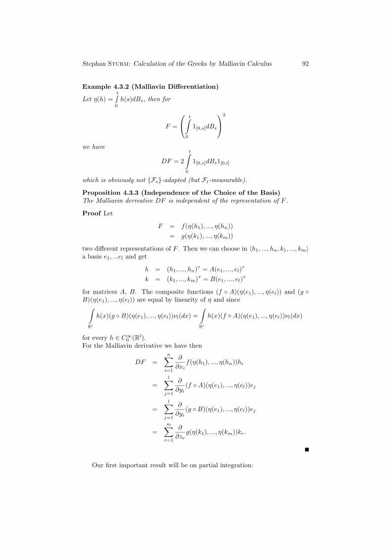
Stephan Sturm: Calculation of the Greeks by Malliavin Calculus 92
Example 4.3.2 (Malliavin Differentiation)
Let η(h) =t∫0
h(s)dBs, then for
F =
t∫0
1[0,s]dBs
2
we have
DF = 2
t∫0
1[0,s]dBs1[0,t]
which is obviously not Fs-adapted (but Ft-measurable).
Proposition 4.3.3 (Independence of the Choice of the Basis)The Malliavin derivative DF is independent of the representation of F .
Proof Let
F = f(η(h1), ..., η(hn))= g(η(k1), ..., η(km))
two different representations of F . Then we can choose in 〈h1, ..., hn, k1, ..., km〉a basis e1, ...el and get
h = (h1, ..., hn)τ = A(e1, ..., el)τ
k = (k1, ..., km)τ = B(e1, ..., el)τ
for matrices A, B. The composite functions (f A)(η(e1), ..., η(el)) and (g B)(η(e1), ..., η(el)) are equal by linearity of η and since∫
Rl
h(x)(g B)(η(e1), ..., η(el))νl(dx) =∫Rl
h(x)(f A)(η(e1), ..., η(el))νl(dx)
for every h ∈ C∞0 (Rl).For the Malliavin derivative we have then
DF =n∑i=1
∂
∂xif(η(h1), ..., η(hn))hi
=l∑
j=1
∂
∂yi(f A)(η(e1), ..., η(el))ej
=l∑
j=1
∂
∂yi(g B)(η(e1), ..., η(el))ej
=m∑r=1
∂
∂zrg(η(k1), ..., η(km))kr.
Our first important result will be on partial integration:
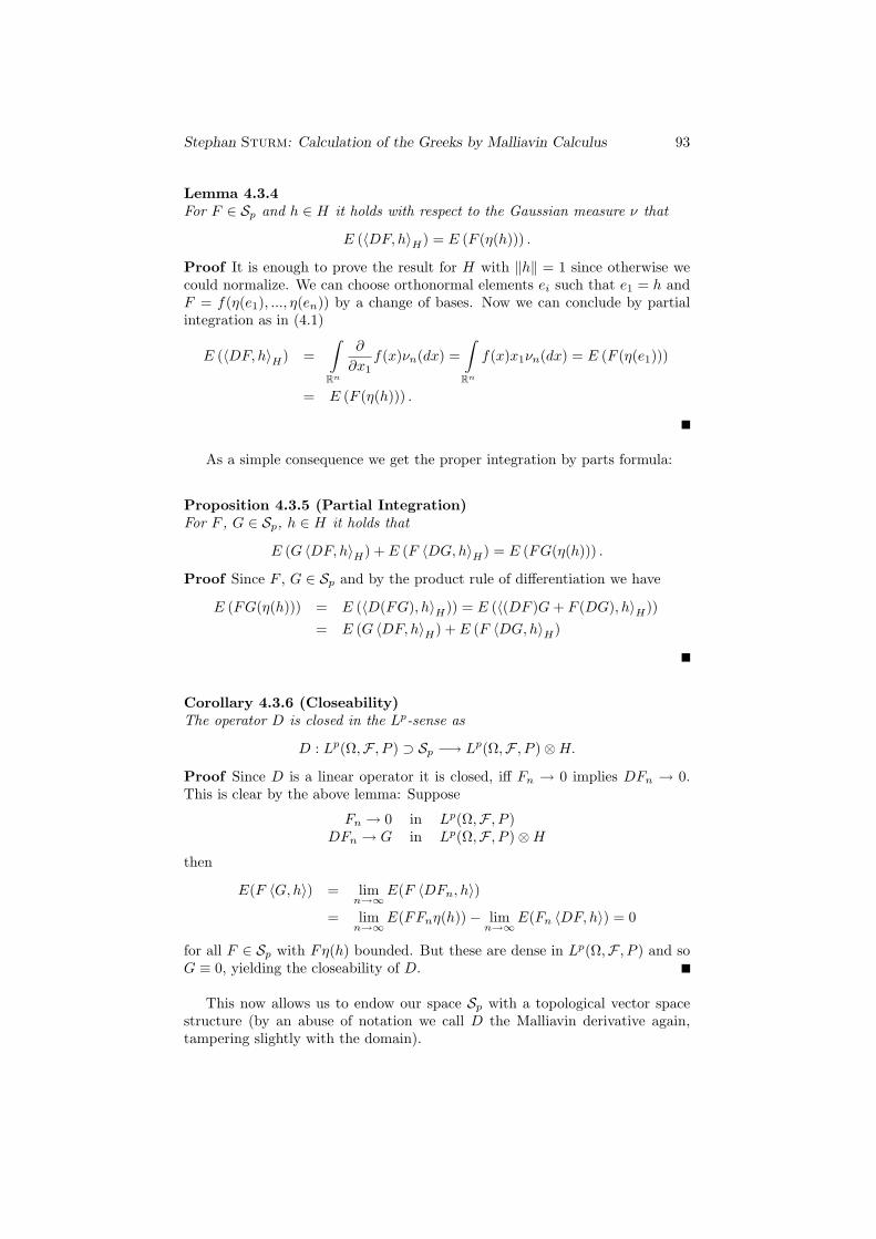
Stephan Sturm: Calculation of the Greeks by Malliavin Calculus 93
Lemma 4.3.4For F ∈ Sp and h ∈ H it holds with respect to the Gaussian measure ν that
E (〈DF, h〉H) = E (F (η(h))) .
Proof It is enough to prove the result for H with ‖h‖ = 1 since otherwise wecould normalize. We can choose orthonormal elements ei such that e1 = h andF = f(η(e1), ..., η(en)) by a change of bases. Now we can conclude by partialintegration as in (4.1)
E (〈DF, h〉H) =∫
Rn
∂
∂x1f(x)νn(dx) =
∫Rn
f(x)x1νn(dx) = E (F (η(e1)))
= E (F (η(h))) .
As a simple consequence we get the proper integration by parts formula:
Proposition 4.3.5 (Partial Integration)For F , G ∈ Sp, h ∈ H it holds that
E (G 〈DF, h〉H) + E (F 〈DG,h〉H) = E (FG(η(h))) .
Proof Since F , G ∈ Sp and by the product rule of differentiation we have
E (FG(η(h))) = E (〈D(FG), h〉H)) = E (〈(DF )G+ F (DG), h〉H))= E (G 〈DF, h〉H) + E (F 〈DG,h〉H)
Corollary 4.3.6 (Closeability)The operator D is closed in the Lp-sense as
D : Lp(Ω,F , P ) ⊃ Sp −→ Lp(Ω,F , P )⊗H.
Proof Since D is a linear operator it is closed, iff Fn → 0 implies DFn → 0.This is clear by the above lemma: Suppose
Fn → 0 in Lp(Ω,F , P )DFn → G in Lp(Ω,F , P )⊗H
then
E(F 〈G, h〉) = limn→∞
E(F 〈DFn, h〉)
= limn→∞
E(FFnη(h))− limn→∞
E(Fn 〈DF, h〉) = 0
for all F ∈ Sp with Fη(h) bounded. But these are dense in Lp(Ω,F , P ) and soG ≡ 0, yielding the closeability of D.
This now allows us to endow our space Sp with a topological vector spacestructure (by an abuse of notation we call D the Malliavin derivative again,tampering slightly with the domain).
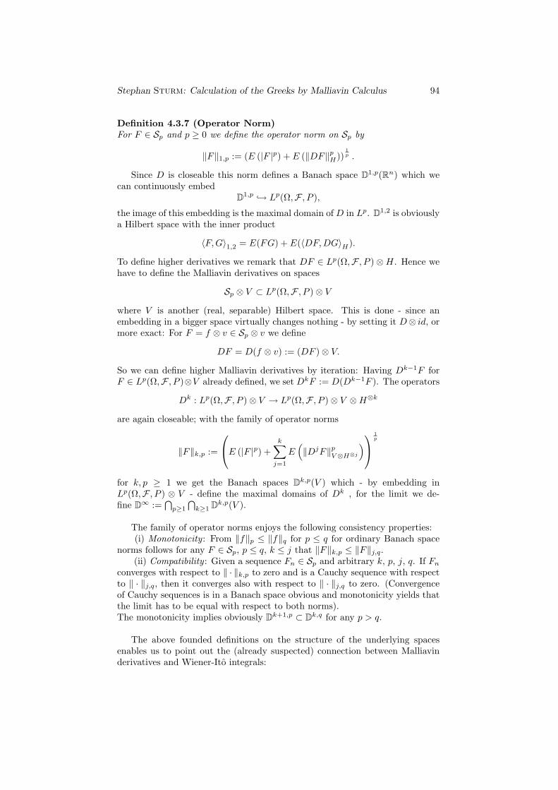
Stephan Sturm: Calculation of the Greeks by Malliavin Calculus 94
Definition 4.3.7 (Operator Norm)For F ∈ Sp and p ≥ 0 we define the operator norm on Sp by
‖F‖1,p := (E (|F |p) + E (‖DF‖pH))1p .
Since D is closeable this norm defines a Banach space D1,p(Rn) which wecan continuously embed
D1,p → Lp(Ω,F , P ),
the image of this embedding is the maximal domain of D in Lp. D1,2 is obviouslya Hilbert space with the inner product
〈F,G〉1,2 = E(FG) + E(〈DF,DG〉H).
To define higher derivatives we remark that DF ∈ Lp(Ω,F , P )⊗H. Hence wehave to define the Malliavin derivatives on spaces
Sp ⊗ V ⊂ Lp(Ω,F , P )⊗ V
where V is another (real, separable) Hilbert space. This is done - since anembedding in a bigger space virtually changes nothing - by setting it D⊗ id, ormore exact: For F = f ⊗ v ∈ Sp ⊗ v we define
DF = D(f ⊗ v) := (DF )⊗ V.
So we can define higher Malliavin derivatives by iteration: Having Dk−1F forF ∈ Lp(Ω,F , P )⊗V already defined, we set DkF := D(Dk−1F ). The operators
Dk : Lp(Ω,F , P )⊗ V → Lp(Ω,F , P )⊗ V ⊗H⊗k
are again closeable; with the family of operator norms
‖F‖k,p :=
E (|F |p) +k∑j=1
E(‖DjF‖pV⊗H⊗j
) 1p
for k, p ≥ 1 we get the Banach spaces Dk,p(V ) which - by embedding inLp(Ω,F , P ) ⊗ V - define the maximal domains of Dk , for the limit we de-fine D∞ :=
⋂p≥1
⋂k≥1 Dk,p(V ).
The family of operator norms enjoys the following consistency properties:(i) Monotonicity : From ‖f‖p ≤ ‖f‖q for p ≤ q for ordinary Banach space
norms follows for any F ∈ Sp, p ≤ q, k ≤ j that ‖F‖k,p ≤ ‖F‖j,q.(ii) Compatibility : Given a sequence Fn ∈ Sp and arbitrary k, p, j, q. If Fn
converges with respect to ‖ · ‖k,p to zero and is a Cauchy sequence with respectto ‖ · ‖j,q, then it converges also with respect to ‖ · ‖j,q to zero. (Convergenceof Cauchy sequences is in a Banach space obvious and monotonicity yields thatthe limit has to be equal with respect to both norms).The monotonicity implies obviously Dk+1,p ⊂ Dk,q for any p > q.
The above founded definitions on the structure of the underlying spacesenables us to point out the (already suspected) connection between Malliavinderivatives and Wiener-Ito integrals:
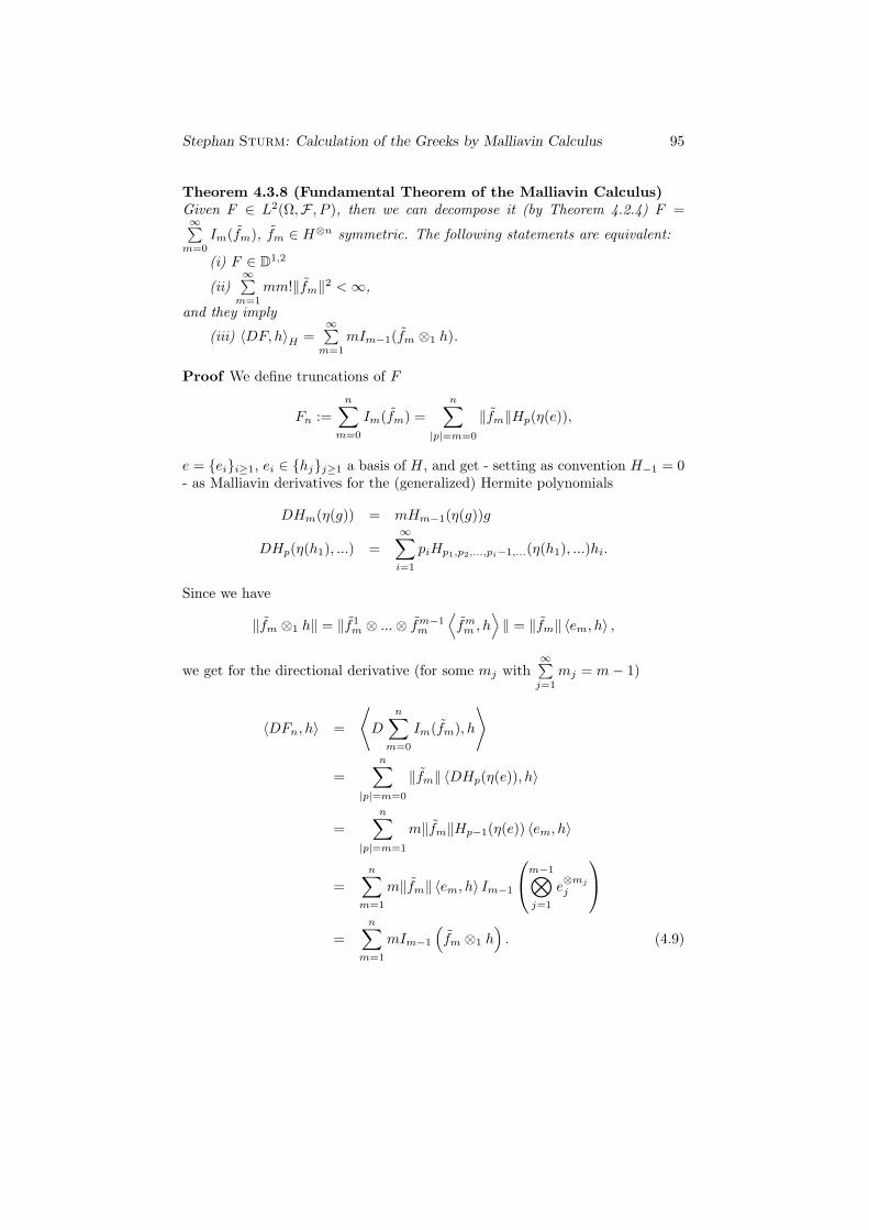
Stephan Sturm: Calculation of the Greeks by Malliavin Calculus 95
Theorem 4.3.8 (Fundamental Theorem of the Malliavin Calculus)Given F ∈ L2(Ω,F , P ), then we can decompose it (by Theorem 4.2.4) F =∞∑m=0
Im(fm), fm ∈ H⊗n symmetric. The following statements are equivalent:
(i) F ∈ D1,2
(ii)∞∑m=1
mm!‖fm‖2 <∞,
and they imply
(iii) 〈DF, h〉H =∞∑m=1
mIm−1(fm ⊗1 h).
Proof We define truncations of F
Fn :=n∑
m=0
Im(fm) =n∑
|p|=m=0
‖fm‖Hp(η(e)),
e = eii≥1, ei ∈ hjj≥1 a basis of H, and get - setting as convention H−1 = 0- as Malliavin derivatives for the (generalized) Hermite polynomials
DHm(η(g)) = mHm−1(η(g))g
DHp(η(h1), ...) =∞∑i=1
piHp1,p2,...,pi−1,...(η(h1), ...)hi.
Since we have
‖fm ⊗1 h‖ = ‖f1m ⊗ ...⊗ fm−1
m
⟨fmm , h
⟩‖ = ‖fm‖ 〈em, h〉 ,
we get for the directional derivative (for some mj with∞∑j=1
mj = m− 1)
〈DFn, h〉 =
⟨D
n∑m=0
Im(fm), h
⟩
=n∑
|p|=m=0
‖fm‖ 〈DHp(η(e)), h〉
=n∑
|p|=m=1
m‖fm‖Hp−1(η(e)) 〈em, h〉
=n∑
m=1
m‖fm‖ 〈em, h〉 Im−1
m−1⊗j=1
e⊗mj
j
=
n∑m=1
mIm−1
(fm ⊗1 h
). (4.9)
Stephan Sturm: Calculation of the Greeks by Malliavin Calculus 96
This result allows us to prove the theorem:(ii) ⇒ (i) By Parseval’s equation we have
‖DFn‖2 =∞∑i=1
E(〈DFn, hi〉2
)=
n∑m=1
∞∑i=1
E
(m2(Im−1(fm ⊗1 hi)
)2)
=n∑
m=1
∞∑i=1
m2(m− 1)!‖fm‖2 〈em, hi〉
=n∑
m=1
mm!‖fm‖2 <∞,
so the sequence ‖DFn‖2 is bounded by∞∑m=1
mm!‖fm‖2, hence it converges;
further F is bounded with respect to the norm ‖ · ‖1,2, so F ∈ D1,2.(i) ⇒ (ii) The required limit regularity we get for DFn by the integration
by parts formula (Proposition 4.3.4) for some G = In(gn) ∈ D1,2:
limn→∞
E(G 〈DFn, h〉) = − limn→∞
E(Fn 〈DG,h〉) + limn→∞
E(FnGη(h))
= −E(F 〈DG,h〉) + E(FGη(h))= E(G 〈DF, h〉).
We can now simply change the direction in the above argument to yield theresult.
(iii) By the above proven boundedness and limit properties it is enough topass in (4.9) to the limit n→∞ to get
〈DF, h〉H =∞∑m=1
mIm−1(fm ⊗1 h).
For the concrete representation H = L2(T,B, µ) (iii) reads
DtF =∞∑m=1
mIm−1(fm(η(h1), ..., η(hm−1), t);
this theorem implies in particular that the Wiener chaoses Hn lie in D1,2.
One of the major tools in dealing with derivatives is usually the chain rule,so let’s have a look how this presents itself in Malliavin calculus:
Proposition 4.3.9 (Chain Rule)Given a differentiable function ϕ ∈ C1 with bounded derivatives. Then it holdsfor fixed p ≥ 1 and F ∈ D1,p(Rn) that ϕ F ∈ D1,p(Rn) and
D(ϕ F ) =n∑i=1
∂
∂xiϕ(F )DF i = 〈∇ϕ(F ), DF 〉 .
Stephan Sturm: Calculation of the Greeks by Malliavin Calculus 97
Proof If ϕ is smooth, the result is a simple consequence of the chain rule inclassical analysis. Otherwise we use the mollifyer ρε (defined by ρ(x) := ce
1x2−1 ,
c chosen such that the integral over rho is one, and ρε(x) := εnρ(εx)) to get asmooth approximation ϕ ∗ ρε for ϕ. Taking smooth approximations F in of F i,then (ϕ ∗ ρε) F in → ϕ F i for ε∧n→∞ in Lp and the closedness of D implies∥∥∥∥∥D(ϕ F )−
n∑i=1
∂
∂xiϕ(F )DF i
∥∥∥∥∥p
≤ ‖D(ϕ F )−D ((ϕ ∗ ρε) F )‖p +
+
∥∥∥∥∥D ((ϕ ∗ ρε) F )−n∑i=1
∂
∂xi(ϕ ∗ ρε)(F )DF in
∥∥∥∥∥p
+
+
∥∥∥∥∥n∑i=1
∂
∂xi(ϕ ∗ ρε)(F )DF in −
n∑i=1
∂
∂xiϕ(F )DF i
∥∥∥∥∥p
→ 0
As consequence we get for instance for ϕ an approximation of x2 thatD(F 2) = 2FDF and by polarization D(FG) = FDG + GDF , F , G ∈ D1,2.Another direct corollary is that this proposition implies that D∞ is a smoothalgebra. To generalize this result we have to prove the following lemma of moretechnical character:
Lemma 4.3.10Given a sequence Fnn≥1 ∈ D1,2 converging to F in L2(Ω,F , P ) fulfilling theboundedness condition
supnE(‖DF‖2H
)<∞,
then F ∈ D1,2 and the sequence of derivatives DFnn≥1 converges weakly toDF in L2(Ω,F , P )⊗H.
Proof It is a direct consequence of the Banach-Alaogu theorem on the weak*-compactness of the unit ball of a dual space that every bounded sequence inthe dual of a separable topological vector space has a converging subsequence.Hence there is a subsequence DFnk
of DFn converging weakly to some α ∈L2(Ω,F , P )⊗H and - projecting the inner product 〈DFnk
, h〉 down to the k-thWiener Chaos - the projections of 〈DFnk
, h〉 converge weakly to 〈α, h〉k, theprojection of 〈α, h〉. Parseval’s identity and the orthogonality of the Wienerchaos decomposition allows us to write for a basis eii≥1 of H
‖α‖2 =∞∑i=1
‖ 〈α, ei〉 ‖2 =∞∑i=1
∞∑k=0
‖ 〈α, ei〉k ‖2.
Since we can decompose F =∞∑m=0
Im(fm) we have by Theorem 4.3.8
‖ 〈α, ei〉k ‖2 = (k + 1)(k + 1)!‖fk‖2,
Stephan Sturm: Calculation of the Greeks by Malliavin Calculus 98
so∞∑k=0
(k + 1)(k + 1)!‖fk‖2 <∞
and hence F ∈ D1,2. It follows that DF = α, the limit of the subsequenceDFnk
; but this argument forces the limit of any weakly converging subsequenceof DFn to be DF , hence the whole sequence DFn converges weakly to DF .
Now we can generalize the chain rule of Malliavin calculus - to even notnecessarily differentiable functions!
Theorem 4.3.11 (Generalized Chain Rule)Given a global Lipschitz function ϕ,
|ϕ(x)− ϕ(y)| ≤ K|x− y| x, y ∈ Rn
and F ∈ D1,2. Then ϕ F ∈ D1,2 and there exists a random vector G ∈ Rn,|G| < K such that
D(ϕ F ) =n∑i=1
GiDF i.
Proof The proof goes nearly analogous as for Proposition 4.3.9, we can takeeven the same mollifyer, ϕ ∗ ρε converges to ϕ uniformly on compacts. Thesequence D ((ϕ ∗ ρε) F ) is bounded in L2(Ω,F , P ) ⊗ H since |∇ (ϕ ∗ ρε)| ≤K for ε large enough. So we can use the previous lemma which asserts thatϕ F ∈ D1,2 and D((ϕ ∗ ρε) F ) → D(ϕ F ) weakly. On the other hand side∇ (ϕ ∗ ρεk
) F converges weakly to some G ∈ Rn, |G| < K. So it is sufficientto take the weak limit in
D((ϕ ∗ ρε) F ) =n∑i=1
∂
∂xi(F )DF i
to yield the result.
Now we will calculate Malliavin derivatives of conditional expectations. There-fore we will use the concrete representation H = L2(T,B, µ) and define theσ-algebra
FA := η(1B) : B ⊂ A ∈ B
which we assume - without loss of generality - to be complete.
Lemma 4.3.12 (Conditioning)
Given F ∈ L2(Ω,F , P ) with decomposition F =∞∑m=0
Im(fm), then it holds for
every A ∈ B that
E(F |FA) =∞∑m=0
Im
(fm1⊗mA
).
Stephan Sturm: Calculation of the Greeks by Malliavin Calculus 99
Proof By their linearity and density it is enough to prove the lemma for func-tions fm of the form 1B1×...×Bm
, the Bm mutually disjoint and of finite measure.For F = Im(fm) we have by (4.7)
E(F |FA) = E (η (1B1) · ... · η (1Bm) |FA)
= E
(m∏i=1
(η (1Bi ∩ 1A) + η (1Bi ∩ 1Ac)) |FA
)
=m∏i=1
η (1Bi ∩ 1A)
= Im(1B1×...×Bm1⊗mA
).
Now we can formulate the theorem:
Theorem 4.3.13 (Conditional Malliavin Derivatives)Let F ∈ D1,2 and A ∈ B, then E(F |FA) ∈ D1,2 and its Malliavin derivative isin Ω× T a.s.
DtE(F |FA) = E(DtF |FA)1A(t).
Proof By the above lemma and Theorem 4.3.8 we have
DtE(F |FA) = Dt
∞∑m=0
Im
(fm1⊗mA
)=
∞∑m=1
mIm−1
(fm(η(h1), ..., η(hm−1), t)1
⊗(m−1)A
)1A(t)
= E
( ∞∑m=1
mIm−1
(fm(η(h1), ..., η(hm−1), t)
∣∣∣FA) 1A(t)
= E(DtF |FA)1A(t).
As last point in this section we prove the Clark-Ocone Haussmann formulawhich shows that any r.v. F ∈ D1,2 can be written as the sum of its expectationand a stochastic integral of conditional expectations of its Malliavin derivative.
Theorem 4.3.14 (Clark-Ocone-Haussmann Formula)
Given F ∈ D1,2 and a one-dimensional Brownian motion Bt, η(h) =∞∫0
h(t)dBt,
then it holds that
F = E(F ) +
∞∫0
E (DtF |Ft) dBt.
Stephan Sturm: Calculation of the Greeks by Malliavin Calculus 100
Proof We use the representation
F =∞∑m=0
Im (fm (η(h1), ..., η(hm))) =∞∑m=0
Im (fm(t1, ..., tm))
and can prove the theorem directly by the fundamental theorem of Malliavincalculus (Theorem 4.3.8), Lemma 4.3.12 and the representation of In as iteratedstochastic integral (Theorem 4.2.6):
∞∫0
E (DtF |Ft) dBt
=
∞∫0
E
(Dt
( ∞∑m=0
Im (fm(t1, ..., tm))
)∣∣∣∣∣Ft)dBt
=
∞∫0
∞∑m=1
mE (Im−1 (fm(t1, ..., tm−1, t) |Ft) dBt
=
∞∫0
∞∑m=1
mIm−1
(fm(t1, ..., tm−1, t)1[0,t]
)dBt
=
∞∫0
∞∑m=1
m!
∞∫0
tm−1∫0
· · ·t2∫
0
fm(t1, ..., tm−1, t)1[0,t]dBt1 · · · dBtm−1
dBt
=∞∑m=1
m!
∞∫0
t∫0
tm−1∫0
· · ·t2∫
0
fm(t1, ..., tm−1, t)dBt1 · · · dBtm−1dBt
=∞∑m=1
Im(fm) =∞∑m=0
Im(fm)− I0(f0)
= F − E(F ).
4.4 The Skorohod Integral
Let’s critical re-examine the core of the introduction to the last section. Toa Gaussian probability space (Ω,F , P ) and an isonormal Gaussian process η :H → L2(Ω,F , P ) (where H was a real and separable Hilbert space) we intro-duced the Malliavin derivative as mapping
D : L2(Ω,F , P ) ⊃ D1,2 → L2(Ω,F , P )⊗H
F 7→ DF.
The operator D is here unbounded, densely defined and (as proven in Corollary4.3.6) closed.
Stephan Sturm: Calculation of the Greeks by Malliavin Calculus 101
So, from a functional analytic viewpoint, all requirements for the existenceof an adjoint operator are fulfilled and one can ask if its introduction makessense in this setting. Indeed there exists an operator
δ = D∗ : L2(Ω,F , P )⊗H ⊃ D1,2 → L2(Ω,F , P )u 7→ δ(u),
the so-called Skorohod integral (or divergence operator). Before going into de-tails we want to give an exact definition.
Definition 4.4.1 (Skorohod Integral)On the domain
D1,2 :=u ∈ L2(Ω,F , P )⊗H : E (〈DF, u〉H) ≤ c(u)‖F‖2
for all F ∈ D1,2 and a constant c depending only on u
the Skorohod integral δ : D1,2 → L2(Ω,F , P ) is defined as operator fulfilling theequation
E (〈DF, u〉H) = E (Fδ(u))
for all F ∈ D1,2.
We see that δ is an unbounded, densely defined operator which is (as adjoint)obviously closed. Clearly the rest of this section will be devoted to the study ofthe Skorohod integral; without much work we can directly see that it coincideswith the isonormal Gaussian process in the deterministic case since by Lemma4.3.4
E (Fδ(1⊗ h)) = E (〈DF, 1⊗ h〉) = E (Fη(h))
for arbitrary h ∈ H.
Lemma 4.4.2Given u ∈ L2(Ω,F , P )⊗H, then we can write it as
u =∞∑m=0
(Im ⊗ id) (fm) (4.10)
for fm ∈ H⊗(m+1) symmetric the first m variables and it holds that
‖u‖2L2(Ω,F,P )⊗H =∞∑m=0
m!‖fm‖2H⊗(m+1) .
Proof The existence of the fm is clear by the chaos expansion (Theorem 4.2.4)and the isometry
L2(Ω,F , P )⊗H '
( ∞⊕m=0
Hm
)⊗H '
∞⊕m=0
(Hm ⊗H)
which follows from the chaos decomposition (Theorem 4.1.10) and the elemen-tary tensor product property from Lemma 1.2.2(iii).For the norm equality we first note that we can - by orthogonality - draw the
Stephan Sturm: Calculation of the Greeks by Malliavin Calculus 102
norm into the sum, the rest is only technical tensor analysis for h ∈ eii≥1, thebasis of H,
‖u‖2L2(Ω,F,P )⊗H = ‖∞∑m=0
(Im ⊗ id) (fm)‖2L2⊗H =∞∑m=0
‖ (Im ⊗ id) (fm)‖2L2⊗H
=∞∑m=0
‖Im(fm ⊗1 h)‖2L2⊗H‖id(h)‖2L2⊗H
=∞∑m=0
m!‖fm‖2H⊗(m+1)‖h‖2H
=∞∑m=0
m!‖fm‖2H⊗(m+1)
Proposition 4.4.3Given u ∈ L2(Ω,F , P ) ⊗ H with the representation (4.10), then the followingconditions are equivalent
(i)∞∑m=0
(m+ 1)!‖fm‖2H⊗(m+1) <∞,
(ii)∞∑m=0
Im+1(fm) converges in L2,
(iii) u ∈ D1,2,and we have the concrete representation of the Skorohod integral
(iv) δ(u) =∞∑m=0
Im+1(fm).
Proof(i) ⇔ (ii) This is clear by
E((Im+1(fm))2
)= (m+ 1)!‖fm‖2H⊗(m+1) .
(i) ⇒ (iii) Assume first that G = In(g) for some symmetric g ∈ H⊗n, thenby orthogonality and since ‖fn‖ = ‖fn‖
E (〈DG,u〉H) = E (〈DIn(g), u〉H) = E (〈n(In−1 ⊗ id)(g), u〉H)= E (〈n(In−1 ⊗ id)(g), (n− 1)(In−1 ⊗ id)(fn−1)〉H)
= n(n− 1)! 〈g, fn−1〉H⊗n = n!⟨g, fn−1
⟩H⊗n
= E(In(g)In(fn−1)
)= E
(GIn(fn−1)
). (4.11)
So under the convergence assumption∞∑m=0
Im+1(fm) = V we have for partialsums
E
(⟨D
k∑n=0
In(gn), u
⟩H
)= E
((k∑
n=0
In(gn)
)(k∑
n=0
In(fn−1)
))
≤ E
((k∑
n=0
In(gn)
)V
),
Stephan Sturm: Calculation of the Greeks by Malliavin Calculus 103
hence by HolderE (〈DF, u〉H) ≤ ‖V ‖2‖F‖2.
This holds for all F with finite chaos decomposition u ∈ D1,2, but since theyare dense, the result follows.
(iii) ⇒ (ii) Calculation (4.11) shows that
E (〈DF, u〉H) = E
( ∞∑m=0
Im(fm−1)F
)<∞,
so convergence follows.(iv) From
E (Gδ(u)) = E (〈DG,u〉H) = E(GIn(fn−1)
)follows that the projections of δ(u) and
∞∑m=0
Im+1(fm) on the n-th Wiener chaos
coincide for every n, so the functions have to be equal.
This representation implies that δ is a linear operator on D1,2 and
E (δ(u)) =
⟨ ∞∑m=0
Im+1(fm), I0(1)
⟩H
= 0
for u ∈ D1,2.
Our next theorem concerns the representation of the processes u:
Proposition 4.4.4 (Representation)Every stochastic process u ∈ L2(Ω,F , P ) ⊗ H has a unique orthogonal decom-position
u = DF + u0
with F ∈ D1,2 and E(⟨DG,u0
⟩H
)= 0 for every G ∈ D1,2.
Proof First we ask which processes u can be represented as DF : This is clearlythe case for all functions which are symmetric in all variables (and not only allbut the last). DF is symmetric in all variables as a sum of Wiener-Ito integrals
(see Theorem 4.3.8), on the other hand side we can set for u =∞∑m=0
(Im⊗id)(fm)
F =∞∑m=0
1m+ 1
Im+1(fm)
which is a series converging D1,2 with
〈DF, h〉H =∞∑m=0
1m+ 1
〈DIm+1(fm), h〉H =∞∑m=0
Im+1(fm ⊗1 h) = 〈u, h〉H
for any h ∈ H. Hence the processes u representable as DF , F ∈ D1,2 form aclosed subspace of L2(Ω,F , P )⊗H and forG ∈ D1,2 we have
⟨DG,u0
⟩H
= 0.
Stephan Sturm: Calculation of the Greeks by Malliavin Calculus 104
Furthermore E(⟨DG,u0
⟩H
)= 0, hence u0 is Skorohod integrable by Defi-
nition 4.4.1 and δ(u0) = 0.
The next results will only apply to special classes of Skorohod integrablefunctions. First we will focus on so-called smooth elementary processes u ∈Sp ⊗ H, hence processes which we can write u =
n∑j=1
Fj ⊗ hj for Fj ∈ Sp and
hj ∈ H.
Proposition 4.4.5 (Smooth Elementary Processes)Smooth elementary processes are Skorohod integrable (Sp ⊗H ⊂ D1,2) and foru as above the divergence is
δ(u) =n∑j=1
Fjη(hj)−n∑j=1
〈DFj , hj〉H .
Proof For an arbitrary F ∈ D1,2 we have
E (Gδ(u)) = E (〈DG,u〉H) =n∑j=1
E(Fj 〈DG,hj〉H
)=
n∑j=1
E (GFjη(hj))−n∑j=1
E(G 〈DFj , hj〉H
)≤ c(u)‖G‖2
by the integration of parts formula (Proposition 4.3.5).
To point out the commutativity property of the Skorohod integral and theMalliavin derivative we have to restrict ourselves to an even smaller class offunctions.
Definition 4.4.6 (L1,2)A stochastic process u ∈ D1,2 is said to be in L1,2, iff u(t) ∈ D1,2 ⊗H.
L1,2 is a Hilbert space with respect to the norm
‖u‖1,2 :=(‖u‖2L2(Ω,F,P )⊗H + ‖Du‖2L2(Ω,F,P )⊗H2
) 12
Proposition 4.4.7 (Commutation)For a process u ∈ L1,2 it holds that
[〈D(·), h〉H , δ(·)]u = 〈u, h〉H .
Proof We can represent u as in (4.10) and get, since the Wiener-Ito integrals
Stephan Sturm: Calculation of the Greeks by Malliavin Calculus 105
are invariant under symmetrization (Theorem 4.2.2),
〈D (δ(u)) , h〉H =
⟨D
∞∑m=0
Im+1(fm), h
⟩H
=∞∑m=0
(m+ 1)Im(fm ⊗1 h)
=∞∑m=0
Im(fm ⊗1 h) +∞∑m=1
mIm(fm ⊗1 h)
=∞∑m=0
Im(fm ⊗1 h) +∞∑m=1
mIm( ˜fm ⊗1 h)
=∞∑m=0
〈(Im ⊗ id) (fm), h〉+ δ
( ∞∑m=1
m (Im−1 ⊗ id) (fm ⊗1 h)
)
= 〈u, h〉H + δ
(⟨D
( ∞∑m=0
(Im ⊗ id) (fm)
), h
⟩H
)= 〈u, h〉H + δ (〈Du, h〉H) .
As a direct consequence of this commutativity property we can calculate thecovariance of the Skorohod integral for L1,2-processes.
Corollary 4.4.8 (Covariance)The covariance of the Skorohod integral is for two processes u, v ∈ L1,2 givenby
E (δ(u)δ(v)) = E (〈u, v〉H) + E (〈Du,Dv〉H)
Proof By the definition of the Skorohod integral (Definition 4.4.1) and thecommutation property (Proposition 4.4.7) it holds for any u ∈ L1,2 with finiteWiener expansion that δ(u) ∈ D1,2 and
E (δ(u)δ(v)) = E (〈D(δ(u)), v)H)= E (〈u, v〉H) + E (〈δ(Du), v〉H)= E (〈u, v〉H) + E (〈Du,Dv〉H) .
In the last step it is implicit that the inner product can - for a concrete rep-resentation - be written as integral and hence by Fubini commutes with theexpectation. But the processes with finite Wiener expansion are dense in L1,2
and the corollary follows.
We are now coming back to a more general class of Skorohod kernels tocalculate the Skorohod integral of the product of a r.v. with a process.
Proposition 4.4.9 (Multipication)
Given u ∈ D1,2 and F ∈ D1,2 such that E(F 2 (δ(u))2
)<∞, then it holds that
δ(Fu) = Fδ(u)− 〈DF, u〉H .
Stephan Sturm: Calculation of the Greeks by Malliavin Calculus 106
Proof Also this proposition we can prove by algebraic means: For G ∈ S0 wehave by the chain rule for Malliavin derivatives (Proposition 4.3.9)
E (GFδ(u)) = E (〈D(GF ), u〉H)= E (〈GDF, u〉H + 〈FDG, u〉H)= E (G 〈DF, u〉H + 〈DG,Fu〉H)= E (G 〈DF, u〉H) + E (Gδ(Fu))
which yields the result since S0 is dense in Sp.
By the definition of the Skorohod integral as counterpart of the Malliavinderivative it seems quite logical to ask for the connection to multiple Wiener-Itointegrals (the climbing up) and Ito integrals (here the connection was estab-lished by Theorem 4.2.6). In fact, we will show that the stochastic Ito integralis nothing else than a special case of the much more general Skorohod integral.But first we have to proof the following Lemma, therefore we have to return toour concrete representation L2(T,B, µ) of H, recalling that µ was a σ-finite andatomless measure.
Lemma 4.4.10Given F ∈ L2(Ω,F , P ), measurable with respect to the σ-algebra
FAc := η(1B) : B ⊂ Ac ∈ B ,
then F1A is Skorohod integrable and
δ(F1A) = Fη(1A).
Proof Assume first that F ∈ D1,2, then it follows by Proposition 4.4.9 on theSkorohod integral of a process multiplied with a r.v. that
δ (F1A) = Fδ (1A)− 〈DtF, 1A〉L2(T )
= Fη(1A)− 〈Dt (E (F |FAc)) , 1A〉L2(T )
= Fη(1A)− 〈E (DtF |FAc) 1Ac(t), 1A〉L2(T )
= Fη(1A)
by the FAc -measurability of F and Theorem 4.3.13. Since D1,2 is dense inL2(Ω,F , P ) and since δ is a closed operator we can pass to the limit whichyields the general result.
Now we can state our theorem on the connection of Ito and Skorohod inte-gral; we do this only in the one dimensional case, but the generalization is notdifficult.
Theorem 4.4.11 (Ito and Skorohod Integrals)The domain of the Skorohod integral contains that of the Ito integral and for
η(h) =∞∫0
h(t)dBt,
u ∈ L2(R≥0 × Ω,B(R≥0)⊗Ft, dt⊗ P ) ⊂ D1,2
Stephan Sturm: Calculation of the Greeks by Malliavin Calculus 107
it holds for a one-dimensional Brownian motion Bt that
δ(u) =
∞∫0
utdBt.
Proof Assume first that u is an elementary step process ut =n∑j=1
Fj1]tj ,tj+1](t)
with Fj ∈ L2(Ω,F ,F[0,tj ], P ) adapted. Then the previous lemma states thatu ∈ D1,2 and
δ(u) = δ
n∑j=1
Fj1]tj ,tj+1](t)
=n∑j=1
Fjη(1]tj ,tj+1](t)
)
=n∑j=1
Fj
∞∫0
1]tj ,tj+1](t)dBt =n∑j=1
Fj(Btj+1 −Btj
)
=
∞∫0
utdBt
by Theorem 4.2.6. By the approximation (Theorem 2.3.3) we can pass to thelimit - since δ is a closed operator - to get the result.
4.5 Malliavin Derivative and First Variation
Till now we developed two different concepts of the derivative of a stochasticprocess: on the one hand side we introduced to a process X satisfying the SDE
dXxt = b(t,Xx
t )dt+ σ(t,Xxt )dBt (4.12)
the first variation process Y = (DX) which satisfies the “derived” SDE
dY xt = b′(t,Xxt )Y xt dt+ σ′(t,Xx
t )Y xt dBt;
in Chapter 3 and now we presented the Malliavin derivative operator D (orconcretely Dt). Not only notational similarities suggest a connection betweenthese two notions... Exactly this connection is what we want to study in thissection, here we can have a first glance on the real goal of the present thesis:The use of Malliavin calculus to gain information on SDEs and the behaviorof their solutions. Since SDEs are highly concrete objects we do not wonderthat we have to work on our concrete representation L2(T,B, µ), µ atomlessand σ-finite, of the Hilbert space.
Proposition 4.5.1 (Malliavin Derivative as SDE Solution)Under the usual conditions on b and σ (as in Chapter 3, Prop 3.3.2) and η(h) =∞∫0
h(t)dBt we have Xxt ∈ D1,2 and the Malliavin derivative DrX
xt satisfies the
Stephan Sturm: Calculation of the Greeks by Malliavin Calculus 108
SDE
DrXxt = σ(r,Xx
r ) +
t∫r
b′(s,Xxs )DrX
xs ds+
t∫r
σ′(s,Xxs )DrX
xs dBs. (4.13)
Proof First we note that Xxt ∈ D1,2 implies DtX
xs = 0 for t > s since
DtXxs = Dt (E(Xx
s |Fs)) = E (DtXxs |Fs) 1[0,s](t)
by Theorem 4.3.13 and hence
Dr
t∫0
usds =
t∫0
Drusds =
t∫r
Drusds
for processes u ∈ D1,2 by approximation with Riemann sums of mollified ele-mentary step processes. Further we have by the commutation property of theSkorohod integral
Dr
t∫0
usdBs =
t∫r
DrusdBs + ur
so that we can try what happens if we “differentiate” directly in the SDE
Xxt = x+
t∫0
b (s,Xxs ) ds+
t∫0
σ (s,Xxs ) dBs.
We get by the chain rule
DrXxt = Dr
t∫0
b (s,Xxs ) ds
+Dr
t∫0
σ (s,Xxs ) dBs
=
t∫r
b′ (s,Xxs )DrX
xs ds+
t∫r
σ′ (s,Xxs )DrX
xs dBs.
This is in no way a result since we know nothing about the solvability yet. Butby exactly the same means as for the first variation (Theorem 3.3.2) we canshow that DrX
xt is the unique solution of the SDE and is jointly continuous
in t and x (with absolute moments of all orders). Furthermore Xxt is by the
Picard-Lindelof iteration really in D1,2.
Now, having an even very strong similarity of the SDEs satisfied by Malliavinderivative and first variation process we will try to establish a direct connection:
Theorem 4.5.2 (Malliavin Derivative and First Variation)Given Xx
t the solution of the SDE (4.12), then it holds for its first variation Y xtthat
DrXxt = Y xt (Y xr )−1σ(r,Xx
r )1[0,t](r).
Stephan Sturm: Calculation of the Greeks by Malliavin Calculus 109
Proof Proposition 4.5.1 implies that DrXxt suffices an (in t) inhomogeneous
equation and it is, by the assumptions on b and σ, a diffeomorphism. So we canwrite it in the form
DrXxt = Bx(r, t)A (4.14)
where Bx(r, t) is a flow and A a matrix derived from the inhomogeneity. Weconclude by (4.13) immediately
A = σ(r,Xxr )1r≤t
and since B is a flow it holds that
Bx(0, t) = Bx(r, t) Bx(0, r)
and hence by invertibility
Bx(r, t) = Bx(0, t) (Bx(0, r))−1.
Therefore equation (4.13) reads by (4.14)
Bx(r, t)A = A+
t∫r
b′(s,Xxs )Bx(r, s)Ads+
t∫r
σ′(s,Xxs )Bx(r, s)AdBs.
Setting r = 0 we have
Bx(0, t) = 1 +
t∫0
b′(s,Xxs )Bx(0, s)ds+
t∫0
σ′(s,Xxs )Bx(0, s)dBs
and - from the uniqueness of the first variation process stated in Theorem 3.3.2- can derive that Bx(0, t) = Y xt a.s. which yields the result.
Corollary 4.5.3Under the above conditions it holds a.s. for ψ ∈ C1
b (R) and r ≤ t ≤ T that
Dr
t∫0
ψ(Xxs )ds =
t∫0
∇ψ(Xxs )Y xs (Y xr )−1σ(r,Xx
r )ds.
Proof Applying the chain rule to the above theorem yields
Drψ(Xxt ) = ∇ψ(Xx
t )DrXxt = ∇ψ(Xx
t )Y xt (Y xr )−1σ(r,Xxr )1[0,t](r)
implying the result.
In this context yet another question rises: Under which conditions does arandom variable have a density? And how smooth is it? Also for this questionMalliavin calculus is the perfect tool to treat it; more, it was developed to proveHormanders celebrated “Sums of the Squares” theorem which is directly con-nected to this question. But all this is beyond the scope of the present work andit is not required for the practical applications in the next chapter. But sincethis is a very good example to see Malliavin calculus at work we will prove theexistence of the density in the one-dimensional case and state the general resultwithout proof.
Stephan Sturm: Calculation of the Greeks by Malliavin Calculus 110
Proposition 4.5.4 (Existence of Densities)Given F ∈ D1,2 and assume that DF
‖DF‖2His Skorohod integrable. Then the law
of F has a continuous and bounded density f given by
f(x) = E
(1F>xδ
(DF
‖DF‖2H
)).
Proof For some reals a < b we define the functions
ψ(y) := 1[a,b](y) and ϕ(y) =
y∫−∞
ψ(z)dz.
Obviously ϕ F ∈ D1,2 and by the chain rule for Malliavin derivatives (Propo-sition 4.3.9) we get
〈D(ϕ F ), DF 〉H = 〈ϕ′(F )DF,DF 〉H = (ψ F )‖DF‖2H .
By the definition of the Skorohod integral this leads to
P (a ≤ F ≤ b) = E(1[a,b](F )
)= E(ψ F )
= E
(1
‖DF‖2H〈D(ϕ F ), DF 〉H
)= E
(⟨D(ϕ F ),
DF
‖DF‖2H
⟩H
)= E
((ϕ F )δ
(DF
‖DF‖2H
))
= E
F∫−∞
ψ(x)dx
δ
(DF
‖DF‖2H
)=
b∫a
E
(1F>xδ
(DF
‖DF‖2H
))dx
by Fubini’s theorem.
In the general case we get:
Theorem 4.5.5 (General Existence and Smoothness of Densities)Given a random vector F , then it has an infinitely differentiable density if thefollowing conditions hold:
(i) Fi ∈ D∞ for all i,(ii) The Malliavin matrix γF := (〈DFi, DFj〉)ij satisfies (det γF )−1 ∈⋂
p>1Lp(Ω,F , P ).
Proof See [Nua 95], p.91.
Chapter 5
Calculating the Greeks
In this chapter we will be concerned with applications of the Malliavin calculusto finance. We want to determine the sensitivity of the price of an option withrespect to small perturbations of the dynamics of the underlying asset, this is,in the language of finance, calculate the Greeks. But first we have to give an(indeed very sketchy) introduction in the theory of pricing options.
5.1 Pricing Options: A very rough Primer
The general background is the question of pricing and hedging derivative se-curities. In opposition to the underlying stocks as shares, bonds, currencies orcommodities which give the holder the direct possession of a good, derivativesgive the holder the right to buy or sell a specified quantity of a stock until aspecified date, the maturity of the derivative for a price specified in advance,the strike price. (In fact everything can get more complicated if we allow alsoderivatives relying on other derivatives...)
While forward contracts or futures give the holder the right and obligationto buy/sell the underlying stock at a specified future date to an in advance fixedprice, options give the holder only the right to buy/sell, but she has no obliga-tion to do so (and will obviously not exercise it if the actual price is lower/higheras the strike price). Options which give the right to buy are named call options,those which give the right to sell put options. Furthermore options are discernedwith respect to their dependence of the payoff: For instance European optionsgive the holder the right (but not the obligation) to buy/sell the underlying forthe strike price (only) at maturity while American options allow this at anydate until maturity. But apart from that a whole bunch of different “exotic”options with rather unusual payoff functions exists...
The practical use of options can be quite diverse: On the one hand side onecan use options as insurance against price hikes, on the other hand side theycan also be used for speculations on increasing or decreasing stock prices. Butthe crucial question is: How to determine their actual value? How do we knowwhich price we are ready to pay for them? The baffling answer is that the fair
111
Stephan Sturm: Calculation of the Greeks by Malliavin Calculus 112
price of an option - under some assumptions - does not depend on the generalexpectations of the behavior of the prices!
The two major assumptions are the following:(i) No Arbitrage: Any opportunity to get a risk-free profit is called an ar-
bitrage opportunity. We assume that there are no such possibilities.(ii) We require that every possible derivative can be hedged, i.e. that we can
construct a portfolio consisting of a risk-free cash bond and underlying stockswhich has exactly the value of the derivative at maturity.
Assuming that the underlying Xxt ∈ Rn satisfies a SDE
dXxt = b(Xx
t )dt+ σ(Xxt )dBt = b(Xx
t )dt+d∑i=1
(σ(Xxt ))i dBt,
the fair price is given by the expectation of the payoff function ϕ(·),
uxt = E(ϕ(Xxt )).
Then the no-arbitrage condition is equal to requiring the existence of a proba-bility measure Q under which
Xx0 = cEQ(Xx
T ),
the risk-neutral probability measure (or equivalent martingale measure). Theconnection to the Girsanov theorem (Theorem 2.5.3) is obvious, the Girsanovtransform deletes the drift and this way forces the independence of the expectedmarket movement such that the price is hence only dependent on th volatilityσ. The market is complete if the equivalent martingale measure is unique.
5.2 The Greeks
The Greeks delta, gamma, theta, rho and the “pseudo-Greek” vega are givenby
∆xt :=
∂uxt∂x
, Γxt :=∂2uxt∂x2
, Θxt :=
∂uxt∂t
, ρxt :=∂uxt∂b
, νxt :=∂uxt∂σ
,
they denote the sensitivity of the price for small perturbations of the initialvalue (respectively the time, the drift and the volatility coefficient). At a firstglance we can see that these usual definitions are for the rho and the vega notsatisfactory in our framework; for constant b and σ (as in the Black-Scholesframework) this is enough, but in our case they are dependent of Xx
t . So wehave to define the derivatives in the directions b (respectively σ by setting thedrift (volatility) coefficient b(Xx
t ) + εb(Xxt ) (σ(Xx
t ) + εσ(Xxt )) and evaluate the
derivatives with respect to ε at ε = 0.
An explicit calculation of the Greeks is not possible in the case of moredifficult payoff functions, so one uses numerical approaches relying on Monte-Carlo estimates (their theory is not in the scope of the present work) for the
Stephan Sturm: Calculation of the Greeks by Malliavin Calculus 113
prices uxt . The easiest methods like finite difference approaches, i.e. for instancefor the delta calculating
ux+εt − uxtε
for small ε, have the disadvantage that they have very poor convergence, inparticular for not so smooth payoff functions ϕ.
One idea of now to overcome this problem is the following which we wantto present for the delta: Assume that the function ϕ : Rn → R has a densityp(t, x, ·) which is dominated by a L1-function and differentiable, then we cancalculate
∇E (ϕ(Xxt )) = ∇
∫Rn
ϕ(y)p(t, x, y)dy
=∫
Rn
ϕ(y)∇p(t, x, y)dy
=∫
Rn
ϕ(y)p(t, x, y)∇p(t, x, y)p(t, x, y)
dy
= E (ϕ(Xxt )π)
where π is the logarithmic derivative
π = ∇ ln p(t, x, y) =∇p(t, x, y)p(t, x, y)
and is called the respective Malliavin weight (for delta). We clearly see thatMalliavin weights are far from being unique since for any π0 with ϕ(Xx
t )⊥π0
the expression π + π0 is also a Malliavin weight.
Since the formula should hold for ϕ(Xxt ) = 1[0,T ](t) too, it follows directly
by ϕ′(Xxt ) = 0 that E(π) = 0 since
E(π) = E(1[0,T ](t)π
)= E (ϕ(Xx
t )π) = E (ϕ′(Xxt )Y xt ) = 0,
so π is a stochastic process with zero expectation. One can guess that it shouldbe something like a stochastic integral
d∑i=1
T∫0
(ψ(Xxt ))idBit
for a process ψ. What we gain by this approach is the boundedness
|∇uxt | ≤ C‖ϕ‖,
which depends only on ϕ (and not on ϕ′!).
Next we want calculate the Malliavin weights (and so the Greeks) in the el-liptic case, following the paper by Fournie, Lasry, Lebuchoux, Lions and Touzi[FLLLT 99].
Stephan Sturm: Calculation of the Greeks by Malliavin Calculus 114
5.3 The Elliptic Case
First we have to lay out the general setting for this purpose. The stochasticprocess Xt0≤t≤T ∈ Rn is driven by the SDE (with respect to an n-dimensionalBrownian motion)
dXxt = b(Xx
t )dt+ σ(Xxt )dBt
where the vector fields b, σi : [0, T ] × Rn → Rn (σi the i-th column of σ,1 ≤ i ≤ n) are C∞-bounded what assures us e.g. the unique existence of thesolution and the first variation. Furthermore we endow σ with a yet strongerregularity property, uniform ellipticity:
Definition 5.3.1 (Uniform Ellipticity)We say that σ satisfies the uniform ellipticity condition, iff there is an ε > 0such that it holds that
(σ(x)ζ)τ (σ(x)ζ) ≥ ε‖ζ‖2
for all t ∈ [0, T ] and x, ζ ∈ Rn.
This implies that the matrix σ is positive definite and all eigenvalues aregreater then ε, hence σ is invertible and the inverse σ−1 is bounded. In ourcase this means that for any bounded function γ : [0, T ] × Rn → Rn, σ−1γ isbounded and the process
(σ−1γ)(Xx
t )
0≤t≤T lies in L2([0, T ]×Ω,Fp, dt⊗P ).
5.3.1 The Rho
The no-arbitrage condition tells us exactly that the drift part vanishes underthe equivalent martingale measure. So we do not have to wonder that we candetermine the rho in a quite general case using Girsanov’s theorem: Given apayoff function ϕ : C([0, T ]) → R satisfying E
(ϕ(Xx
t )2)< ∞. We define the
perturbed process Xxt 0≤t≤T by
dXxt =
(b(Xx
t ) + εb(Xxt ))dt+ σ(Xx
t )dBt
for small ε and b : [0, T ]× Rn → Rn bounded and further
ξxt := e−ε
n∑i=1
t∫0((σ−1b)(Xx
s ))idBi
s− ε22
n∑i=1
t∫0
(((σ−1b)(Xx
s ))i)2ds
which is a true martingale by Novikov’s condition (Corollary 2.5.4) since (σ−1b)is bounded.
Our aim is to derive the expectation
uxt := E(ϕ(Xx
t ))
and evaluate it at ε = 0, this gives the price sensitivity with respect to theinterest rate (which corresponds with the drift part), the ρ.
Stephan Sturm: Calculation of the Greeks by Malliavin Calculus 115
Proposition 5.3.2 (Rho)The function ε 7→ uxt is differentiable in ε = 0 and it holds that
ρxt =∂uxt∂ε
∣∣∣∣ε=0
= E
ϕ(Xxt )
n∑i=1
T∫0
((σ−1b)(Xx
t ))idBit
.
Proof (i) Since E(ξxT ) = 1 (by Novikov’s condition) we can define a proba-bility measure Q with dQ
dP = (ξxT )−1 which is, in fact, even equivalent to P sinceξxT > 0 a.s. So we have for
Bt := Bt + ε
t∫0
(σ−1b)(Xxs )ds
ξxt := e−ε
n∑i=1
t∫0((σ−1b)(Xx
s ))idBi
t− ε22
n∑i=1
t∫0
(((σ−1b)(Xx
s ))i)2ds
by the Radon-Nikodym theorem (Theorem 2.5.1)
uxt = E(ϕ(Xx
t ))
= EQ
(ϕ(Xx
t )ξxT)
= E (ϕ(Xxt )ξxT )
since the joint distributions of (Xxt , Bt) under Q and of (Xx
t , Bt) under P coin-cide by definition of Xx
t and Bt.(ii) Since ξxt is a stochastic exponential we have
dξxt = εn∑i=1
ξxt
((σ−1b)(Xx
t ))idBt
and since ξxt = 1 for ε = 0
1ε(ξxT − 1) =
n∑i=1
T∫0
ξxt
((σ−1b)(Xx
t ))idBit.
For ε→ 0 this yields the L2-convergence
1ε(ξxT − 1) →
n∑i=1
T∫0
((σ−1b)(Xx
t ))idBit.
Stephan Sturm: Calculation of the Greeks by Malliavin Calculus 116
(iii) Since E(ϕ(Xx
t )2)<∞ we can conclude by Cauchy’s inequality∣∣∣∣∣∣ u
xt − uxtε
− E
ϕ(Xxt )
n∑i=1
T∫0
((σ−1b)(Xx
t ))idBit
∣∣∣∣∣∣=
∣∣∣∣∣∣E(ϕ(Xx
t )(ξxT − 1)
ε
)− E
ϕ(Xxt )
n∑i=1
T∫0
((σ−1b)(Xx
t ))idBit
∣∣∣∣∣∣=
∣∣∣∣∣∣Eϕ(Xx
t )
(ξxT − 1)ε
−n∑i=1
T∫0
((σ−1b)(Xx
t ))idBit
∣∣∣∣∣∣≤
(E(ϕ(Xx
t )2)) 1
2
E (ξxT − 1)
ε−
n∑i=1
T∫0
((σ−1b)(Xx
t ))idBit
2
12
−→ 0
for ε→ 0 which yields by limε→0
uxt−u
xt
ε = ∂uxt
∂ε
∣∣∣ε=0
the result.
That we could calculate the rho in a Girsanov way was a direct consequenceof the no-arbitrage assumption (and hence the existence of an equivalent mar-tingale measure which annihilates the drift), in the case of the delta and thevega we have to find other methods. Here Malliavin calculus enters the sceneand will show that it is the perfect tool to calculate the Greeks.
5.3.2 The Delta
For the delta we consider the case of a payoff function ϕ : Rn×m → R dependingon m points in time, 0 < t1 ≤ ... ≤ tm < T , requiring obviously
E(ϕ(Xxt1 , ..., X
xtm
)2)<∞.
Then the price of the derivative is given by
uxt := E(ϕ(Xxt1 , ..., X
xtm
))and for the set Γ∆
m of square integrable functions with integral up to the timesti equal one, i.e.
Γ∆m :=
a ∈ L2([0, T ]) :
ti∫0
atdt = 1, i ∈ 1, ...,m
we get the following result for the Delta:
Proposition 5.3.3 (Delta)Assuming σ uniformly elliptic it holds for any a ∈ Γ∆
m that
∆xt = ∇uxt = E
ϕ(Xxt1 , ...X
xtm)
n∑i=1
T∫0
at
((σ−1(Xx
t ))iY xt
)τdBit
.
Stephan Sturm: Calculation of the Greeks by Malliavin Calculus 117
Proof In a first step we show that the result for the case that ϕ ∈ C1(Rn×m,R)and ‖∇ϕ‖ <∞ where ∇j will denote the partial derivative with respect to thej-th argument.
(i) We note that by Theorem 4.5.2 follows immediately for a ∈ Γ∆m
T∫0
(DtXxti)atσ
−1(Xxt )Y xt dt =
ti∫0
Y xti (Yxt )−1σ(Xx
t )atσ−1(Xxt )Y xt dt
=
ti∫0
Y xtiatdt = Y xti
ti∫0
atdt = Y xti . (5.1)
(ii) Our aim is to express the gradient of uxt by differentiating inside theexpectation: Since ϕ is continuously differentiable we have for h ∈ Rn, |h| → 0the a.s. convergence for the directional derivative
ϕ(Xx+ht1 , ...Xx+h
tm )− ϕ(Xxt1 , ...X
xtm)
‖h‖−
(m∑i=1
(∇τi ϕ(Xx
t1 , ...Xxtm)Y xti
))h
‖h‖→ 0
(5.2)Both terms are uniformly integrable; for the second one this is clear by theassumption of the bounded gradient, the first can be estimated by∥∥∥∥∥ϕ(Xx+h
t1 , ...Xx+htm )− ϕ(Xx
t1 , ...Xxtm)
‖h‖
∥∥∥∥∥ ≤ ‖∇ϕ‖m∑k=1
∥∥Xx+htk
−Xxtk
∥∥‖h‖
<∞
where the right term is clearly u.i. by the boundedness of the gradient and thejoint continuity of the first variation (Theorem 3.3.2, 3.3.3). So (5.2) converges(by Lebesgue’s dominated convergence) also in the L1-sense and we get theresult.
(iii) Thereon we can now perform our Malliavin-theoretic calculations:
∇τuxt = E
m∑j=1
∇τjϕ(Xx
t1 , ...Xxtm)Y xtj
= E
T∫0
m∑j=1
∇τjϕ(Xx
t1 , ...Xxtm)(DtX
xtj )atσ
−1(Xxt )Y xt dt
= E
T∫0
Dtϕ(Xxt1 , ...X
xtm)atσ−1(Xx
t )Y xt dt
= E
(ϕ(Xx
t1 , ...Xxtm)δ
(atσ
−1(Xxt )Y xt
))= E
ϕ(Xxt1 , ...X
xtm)
n∑i=1
T∫0
at(σ−1(Xx
t ))iY xt dB
it
by (5.1), the chain rule of Malliavin calculus (Proposition 4.3.9) and the def-inition of the Skorohod integral, which could in fact - since for any concrete
Stephan Sturm: Calculation of the Greeks by Malliavin Calculus 118
function at the process atσ−1(Xxt )Y xt is progressively measurable - be written
as classical Ito integral.(iv) We have to generalize the result to arbitrary square-integrable ϕ’s:
Since C∞0 is dense in L2(Ω,F , P ) (see begin of Section 4.3) we can choose asequence ϕk therein converging to ϕ and define
uk := E(ϕn(Xx
t1 , ..., Xxtm)).
Obviously we have for any initial value x
uk −→ u,
on the other hand side for the uk the proposition is already proved and wecan conclude by the Cauchy-Schwarz inequality - using the abbreviation ϕx :=ϕk(Xx
t1 , ...Xxtm)− ϕ(Xx
t1 , ...Xxtm) - that∣∣∣∣∣∣∇uk − E
ϕ(Xxt1 , ...X
xtm)
n∑i=1
T∫0
at
((σ−1(Xx
t ))iY xt
)τdBit
∣∣∣∣∣∣≤
∣∣∣∣∣∣Eϕx n∑
i=1
T∫0
at
((σ−1(Xx
t ))iY xt
)τdBit
∣∣∣∣∣∣≤
∥∥∥E (ϕx)2∥∥∥ 1
2
∥∥∥∥∥∥∥E n∑i=1
T∫0
at
((σ−1(Xx
t ))iY xt
)τdBit
2∥∥∥∥∥∥∥
12
→ 0
uniformly on compacts for k →∞, so
uk −→ u
∇uk −→ E
ϕ(Xxt1 , ...X
xtm)
n∑i=1
T∫0
at
((σ−1(Xx
t ))iY xt
)τdBit
,
hence u is continuously differentiable and the proposition holds in the generalcase as well.
By the same arguments we can obviously derive formulae for higher deriva-tives, for instance we can get the gamma, the second derivative with respect tothe initial value.
5.3.3 The Vega
As for the previous Greeks we start by laying out the concrete framework, nearlythe same as for delta. Additionally we define the set Γν
m by
Γνm :=
a ∈ L2([0, T ]) :
ti∫ti−1
atdt = 1, i ∈ 1, ...,m, t0 := 0
Stephan Sturm: Calculation of the Greeks by Malliavin Calculus 119
and the (volatility) perturbed process Xxt by
dXxt := b(Xx
t )dt+(σ(Xx
t ) + εσ(Xxt ))dBt
where we have to require that the perturbed diffusion matrix σ+εσ also satisfiesthe uniform ellipticity condition:
((σ(x) + εσ(x)) ζ)τ ((σ(x) + εσ(x)) ζ) ≥ η|ζ|2.
Besides the first variation with respect to the initial value we define that withrespect to ε by
dZxt := b′(Xxt )Zxt dt+
(σ(Xx
t ))idBit +
n∑i=1
(σ′(Xx
t ) + εσ(Xxt ))iZxt dB
it
with initial value Zx0 = 0, the null column vector. Zxt exists uniquely due toPicard-Lindelof and we will write Zxt for Zxt
∣∣∣ε=0
. Furthermore we define the
processes βt and βat by
βt := (Y xt )−1Zxt
βat :=m∑i=1
at(βti − βti−1)1[ti−1,ti].
Proposition 5.3.4 (Vega)Under the above assumptions the function ε→ uxt is differentiable in ε = 0 andit holds that
νxt =∂uxt∂ε
∣∣∣∣ε=0
= E(ϕ(Xx
t1 , ...Xxtm)δ
(σ−1(Xx
t )Y xt βaT
)).
Proof We note that it is enough to prove the proposition for ϕ ∈ C1b (Rn×m,R)
since the generalization is completely analogous to that of delta.(i) We want to prove that βt ∈ D1,2 (and hence also βaT ): The inverse
(Y xt )−1 of the first variation process is given by the SDE
dW xt = W x
t
(−b′(Xx
t ) +n∑i=1
((σ′(Xx
t ))i)2)dt−W x
t
n∑i=1
(σ′(Xxt ))i dBit (5.3)
with initial value W x0 = In, since
d 〈Y x,W x〉t =
⟨n∑i=1
(σ′(Xxt ))i Y xt dB
it,−W x
t
n∑i=1
(σ′(Xxt ))i dBit
⟩
= −n∑i=1
(σ′(Xxt ))i Y xt W
xt (σ′(Xx
t ))i dt
and hence by partial integration (Proposition 2.4.30)
dY xt Wxt = dY x0 W
x0 + Y xt dW
xt +W x
t dYxt + d 〈Y x,W x〉t
= Y xt Wxt
(n∑i=1
(σ′(Xxt ))i
)2
dt−n∑i=1
(σ′(Xxt ))i Y xt W
xt (σ′(Xx
t ))i dt
Stephan Sturm: Calculation of the Greeks by Malliavin Calculus 120
which implies that W xt = (Y xt )−1 is a solution of (5.3) which is unique due to
a Picard-Lindelof argument. By the C∞-boundedness of the vector fields are(Y xt )−1 and Zxt in D1,2 and the Cauchy inequality∣∣(Y xt )−1Zxt
∣∣2 ≤ E((
(Y xt )−1)2)
E((Zxt )2
)yields - by the closedness of D (Corollary 4.3.6) - the result.
(ii) By Theorem 4.5.2 and the definition of βat it follows for any a ∈ Γνm
that
T∫0
DtXxtiσ
−1(Xxt )Y xt β
aT dt =
ti∫0
Y xti βaT dt = Y xti
i∑k=1
tk∫tk−1
at(βtk − βtk−1
)dt
= Y xti
i∑k=1
(βtk − βtk−1
) tk∫tk−1
atdt = Y xtiβti = Zxti .
(iii) Analogously to point (ii) of the proof of the delta formula we can -since Xx
t is as flow a continuously differentiable function (with respect to ε) -conclude in the L1-sense
∂uxt∂ε
∣∣∣∣ε=0
= E
(m∑i=1
∇τi ϕ(Xx
t1 , ...Xxtm)Zxti
).
(iv) To finish we will naturally use Malliavin calculus...
∂uxt∂ε
∣∣∣∣ε=0
= E
(m∑i=1
∇τi ϕ(Xx
t1 , ...Xxtm)Zxti
)
= E
T∫0
m∑i=1
∇τi ϕ(Xx
t1 , ...Xxtm)DtX
xtiσ
−1(Xxt )Y xt β
aT dt
= E
T∫0
Dtϕ(Xxt1 , ...X
xtm)σ−1(Xx
t )Y xt βaT dt
= E
(ϕ(Xx
t1 , ...Xxtm)δ
(σ−1(Xx
t )Y xt βaT
))by (ii), the chain rule (Proposition 4.3.9) and since βaT ∈ D1,2 (by (i)). Further-more σ−1(Xx
t )Y xt ∈ D1,2 and
E
((βaT
)2 (δ(σ−1(Xx
t )Y xt))2) ≤ (E (βaT))2 (
E(δ(σ−1(Xx
t )Y xt)))2
<∞
assures by 4.4.9 the Skorohod-integrability of the kernel.
The Skorohod integral is not an Ito integral since βaT is FT -measurablethough not Ft-adapted. But the Proposition 4.4.9 even assures us a repre-
Stephan Sturm: Calculation of the Greeks by Malliavin Calculus 121
sentation of the Skorohod integral in terms of classical Ito-calculus, we have
δ(σ−1(Xx
t )Y xt βaT
)=
(βaT
)τ n∑i=1
T∫0
(σ−1(Xx
t ))iY xt dB
it −
n∑i=1
n∑j=1
T∫0
(Dtβ
aT
)ij (σ−1(Xx
t )Y xt)ji
dt
=(βaT
)τ n∑i=1
T∫0
(σ−1(Xx
t ))iY xt dB
it −
T∫0
tr(Dtβ
aTσ
−1(Xxt )Y xt
)dt.
We remark here that we calculated the delta and the vega for ϕ depending onfinitely many points. That one can not generalize these proofs straight forwardto continuous dependencies is clear by looking at sequences t1k
→ 0 for deltaand tik → ti for vega, k →∞.
5.4 Beyond Ellipticity
In this chapter we will drop the ellipticity assumption what means not onlyto give up the uniform ellipticity condition - which assured us the necessaryinvertibility of the matrices - but also to admit arbitrary (hence d) Brownianmotions. (Remark that in the last chapter the number of Brownian motionswas exactly the dimension of the process to produce (invertible) square (n× n)matrices).
For commodity we will here use Stratonovich calculus, hence the SDE isgiven by
dXxt = b(Xx
t )dt+d∑i=1
(σ(Xxt ))i dBit,
b and σi again C∞-bounded. Further we define the sets
V0 :=σ1, ..., σd
Vk :=
[V i, V j ] : V i ∈ Vr, V j ∈ Vs, 0 ≤ r ≤ s < k
V∞ :=
∞⋃k=0
Vk
and assume that the span of V∞ has constant rank
rk (〈V∞〉) = R ≤ n
and b ∈ 〈V∞〉.
So the first variation as n × n matrix exists by a Picard-Lindelof argumentand it is given by
dY xt = b′(Xxt )Y xt dt+
d∑i=1
(σ′(Xxt ))i Y xt dBit;
Stephan Sturm: Calculation of the Greeks by Malliavin Calculus 122
by the same considerations as in part (i) of the proof of Proposition 5.3.4 theinverse (Y xt )−1 exists a.s. In this context the Malliavin derivative DsX
xt is a
n× d matrix which satisfies
DsXxt = Y xt (Y xs )−1σ(Xx
s )1[0,t](s) (5.4)
and conversely the Skorohod integral of a d×n (Skorohod integrable) matrix isan n-dimensional column vector.
We remember the Malliavin matrix γ of Theorem 4.5.5,
γ = γt :=(⟨Ds(Xx
t )i, Ds(Xxt )j⟩)ij
=
t∫0
(DsXxt )(DsX
xt )τds,
which is for R = n by [Nua] p.116, Lemma 2.3.1 invertible, so is the matrix Ctdefined
Ct :=
t∫0
((Y xs )−1
σ(Xxs ))(
(Y xs )−1σ(Xx
s ))τds
which is via invertible matrices related to γ by (5.4)
γt = Y xt Ct(Yxt )τ . (5.5)
As the last point we introduce for fixed t the set Axt by
Axt :=
a ∈ D1,2 :
t∫0
(Y xs )−1σ(Xxs )asds = In
=
a ∈ D1,2 :
t∫0
(DsXxt )asds = Y xt
(5.6)
again by (5.4) which consists of d × n matrix valued processes satisfying theintegral condition. Now we can present the central theorem:
Theorem 5.4.1 (Hypoellliptic Delta)If R = n, then Axt 6= ∅ for all x ∈ Rn, t > 0 and it holds for ϕ : Rn → R that
∆xt = E
(ϕ(Xx
t )(δ((
(Y xs )−1σ(Xxs ))τC−1t
))τ).
Proof(i) The non-emptiness of Axt we show directly by stating an element whose
existence is clear:as := (DsX
xt )τγ−1
t Y xt .
This is an element of Axt according to (5.4) since
t∫0
(DsXxt )(DsX
xt )τγ−1
t Y xt ds =
t∫0
(DsXxt )(DsX
xt )τdsγ−1
t Y xt
= γtγ−1t Y xt = Y xt .
Stephan Sturm: Calculation of the Greeks by Malliavin Calculus 123
(ii) Using (5.3) and (5.4) we can write
as = (DsXxt )τγ−1
t Y xt
= (Y xt (Y xs )−1σ(Xxs ))τ (Y xt Ct(Y
xt )τ )−1
Y xt
=((Y xs )−1σ(Xx
s ))τC−1t .
(iii) Since there are no differences to the elliptic case of the delta (Proposition5.2.3(ii)) we can interchange gradient and expectation and hence
∇τuxt = E (∇τϕ(Xxt )Y xt )
= E
∇τϕ(Xxt )
t∫0
(DsXxt )asds
= E
t∫0
∇τϕ(Xxt )(DsX
xt )asds
= E
t∫0
(Dsϕ(Xxt )) asds
= E (ϕ(Xx
t )δ(as))
and so by (ii)
∆xt = E (ϕ(Xx
t ) (δ(as))τ ) = E
(ϕ(Xx
t )(δ((
(Y xs )−1σ(Xxs ))τC−1t
))τ)
Solving the Skorohod integral we get
δ((
(Y xs )−1σ(Xxs ))τC−1t
)=
(C−1t
)τ t∫0
((Y xs )−1σ(Xx
s ))τdBis
−n∑i=1
d∑j=1
t∫0
(Ds(C−1
t )τ)kij ((
(Y xs )−1σ(Xxs ))τ)ji
ds
=(C−1t
)τ t∫0
((Y xs )−1σ(Xx
s ))τdBis
−t∫
0
tr((Ds(C−1
t )τ) (
(Y xs )−1σ(Xxs ))τ)
ds.
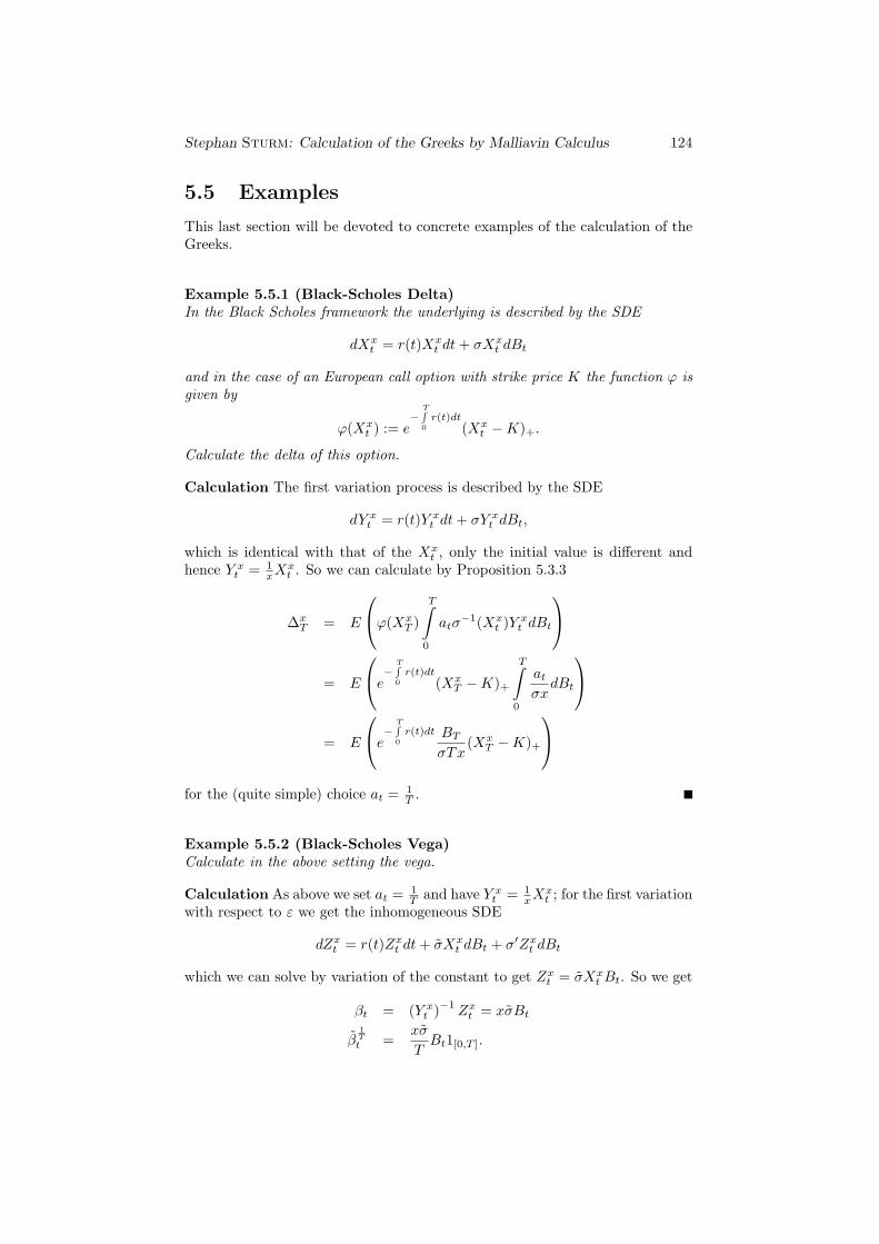
Stephan Sturm: Calculation of the Greeks by Malliavin Calculus 124
5.5 Examples
This last section will be devoted to concrete examples of the calculation of theGreeks.
Example 5.5.1 (Black-Scholes Delta)In the Black Scholes framework the underlying is described by the SDE
dXxt = r(t)Xx
t dt+ σXxt dBt
and in the case of an European call option with strike price K the function ϕ isgiven by
ϕ(Xxt ) := e
−T∫0r(t)dt
(Xxt −K)+.
Calculate the delta of this option.
Calculation The first variation process is described by the SDE
dY xt = r(t)Y xt dt+ σY xt dBt,
which is identical with that of the Xxt , only the initial value is different and
hence Y xt = 1xX
xt . So we can calculate by Proposition 5.3.3
∆xT = E
ϕ(XxT )
T∫0
atσ−1(Xx
t )Y xt dBt
= E
e− T∫0r(t)dt
(XxT −K)+
T∫0
atσxdBt
= E
e− T∫0r(t)dt BT
σTx(Xx
T −K)+
for the (quite simple) choice at = 1
T .
Example 5.5.2 (Black-Scholes Vega)Calculate in the above setting the vega.
Calculation As above we set at = 1T and have Y xt = 1
xXxt ; for the first variation
with respect to ε we get the inhomogeneous SDE
dZxt = r(t)Zxt dt+ σXxt dBt + σ′Zxt dBt
which we can solve by variation of the constant to get Zxt = σXxt Bt. So we get
βt = (Y xt )−1Zxt = xσBt
β1Tt =
xσ
TBt1[0,T ].
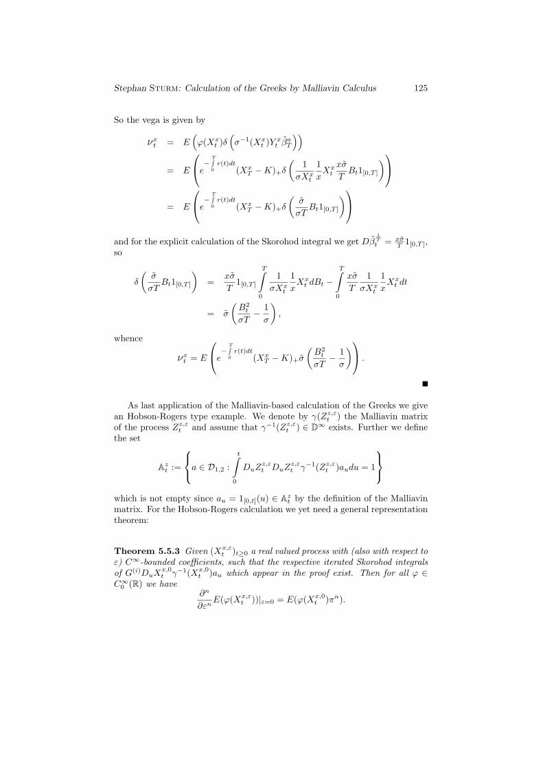
Stephan Sturm: Calculation of the Greeks by Malliavin Calculus 125
So the vega is given by
νxt = E(ϕ(Xx
t )δ(σ−1(Xx
t )Y xt βaT
))= E
e− T∫0r(t)dt
(XxT −K)+δ
(1
σXxt
1xXxt
xσ
TBt1[0,T ]
)= E
e− T∫0r(t)dt
(XxT −K)+δ
(σ
σTBt1[0,T ]
)and for the explicit calculation of the Skorohod integral we get Dβ
1Tt = xσ
T 1[0,T ],so
δ
(σ
σTBt1[0,T ]
)=
xσ
T1[0,T ]
T∫0
1σXx
t
1xXxt dBt −
T∫0
xσ
T
1σXx
t
1xXxt dt
= σ
(B2t
σT− 1σ
),
whence
νxt = E
e− T∫0r(t)dt
(XxT −K)+σ
(B2t
σT− 1σ
) .
As last application of the Malliavin-based calculation of the Greeks we givean Hobson-Rogers type example. We denote by γ(Zz,εt ) the Malliavin matrixof the process Zz,εt and assume that γ−1(Zz,εt ) ∈ D∞ exists. Further we definethe set
Azt :=
a ∈ D1,2 :
t∫0
DuZz,εt DuZ
z,εt γ−1(Zz,εt )audu = 1
which is not empty since au = 1[0,t](u) ∈ Azt by the definition of the Malliavinmatrix. For the Hobson-Rogers calculation we yet need a general representationtheorem:
Theorem 5.5.3 Given (Xx,εt )t≥0 a real valued process with (also with respect to
ε) C∞-bounded coefficients, such that the respective iterated Skorohod integralsof G(i)DuX
x,0t γ−1(Xx,0
t )au which appear in the proof exist. Then for all ϕ ∈C∞0 (R) we have
∂n
∂εnE(ϕ(Xx,ε
t ))|ε=0 = E(ϕ(Xx,0t )πn).
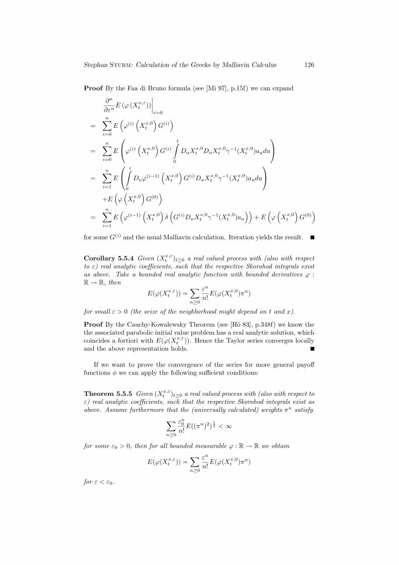
Stephan Sturm: Calculation of the Greeks by Malliavin Calculus 126
Proof By the Faa di Bruno formula (see [Mi 97], p.15f) we can expand
∂n
∂εnE (ϕ (Xx,ε
t ))∣∣∣∣ε=0
=n∑i=0
E(ϕ(i)
(Xx,0t
)G(i)
)
=n∑i=0
E
ϕ(i)(Xx,0t
)G(i)
t∫0
DuXx,0t DuX
x,0t γ−1(Xx,0
t )audu
=
n∑i=1
E
t∫0
Duϕ(i−1)
(Xx,0t
)G(i)DuX
x,0t γ−1(Xx,0
t )audu
+E
(ϕ(Xx,0t
)G(0)
)=
n∑i=1
E(ϕ(i−1)
(Xx,0t
)δ(G(i)DuX
x,0t γ−1(Xx,0
t )au))
+ E(ϕ(Xx,0t
)G(0)
)for some G(i) and the usual Malliavin calculation. Iteration yields the result.
Corollary 5.5.4 Given (Xx,εt )t≥0 a real valued process with (also with respect
to ε) real analytic coefficients, such that the respective Skorohod integrals existas above. Take a bounded real analytic function with bounded derivatives ϕ :R → R, then
E(ϕ(Xx,εt )) =
∑n≥0
εn
n!E(ϕ(Xx,0
t )πn)
for small ε > 0 (the seize of the neighborhood might depend on t and x).
Proof By the Cauchy-Kowalewsky Theorem (see [Ho 83], p.348f) we know thethe associated parabolic initial value problem has a real analytic solution, whichcoincides a fortiori with E(ϕ(Xx,ε
t )). Hence the Taylor series converges locallyand the above representation holds.
If we want to prove the convergence of the series for more general payofffunctions φ we can apply the following sufficient conditions:
Theorem 5.5.5 Given (Xx,εt )t≥0 a real valued process with (also with respect to
ε) real analytic coefficients, such that the respective Skorohod integrals exist asabove. Assume furthermore that the (universally calculated) weights πn satisfy∑
n≥0
εn0n!E((πn)2)
12 <∞
for some ε0 > 0, then for all bounded measurable ϕ : R → R we obtain
E(ϕ(Xx,εt )) =
∑n≥0
εn
n!E(ϕ(Xx,0
t )πn)
for ε < ε0.
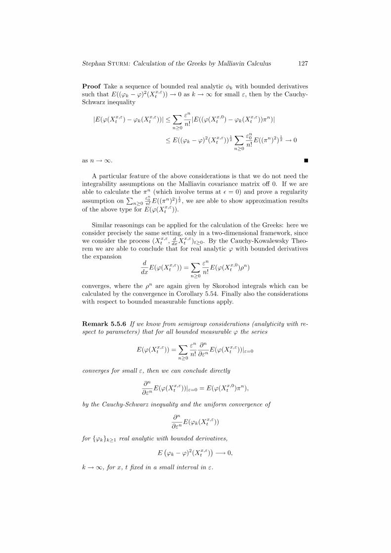
Stephan Sturm: Calculation of the Greeks by Malliavin Calculus 127
Proof Take a sequence of bounded real analytic φk with bounded derivativessuch that E((ϕk − ϕ)2(Xx,ε
t )) → 0 as k →∞ for small ε, then by the Cauchy-Schwarz inequality
|E(ϕ(Xx,εt )− ϕk(X
x,εt ))| ≤
∑n≥0
εn
n!|E((ϕ(Xx,0
t )− ϕk(Xx,εt ))πn)|
≤ E((ϕk − ϕ)2(Xx,εt ))
12
∑n≥0
εn0n!E((πn)2)
12 → 0
as n→∞.
A particular feature of the above considerations is that we do not need theintegrability assumptions on the Malliavin covariance matrix off 0. If we areable to calculate the πn (which involve terms at ε = 0) and prove a regularityassumption on
∑n≥0
εn0n!E((πn)2)
12 , we are able to show approximation results
of the above type for E(ϕ(Xx,εt )).
Similar reasonings can be applied for the calculation of the Greeks: here weconsider precisely the same setting, only in a two-dimensional framework, sincewe consider the process (Xx,ε
t , ddxXx,εt )t≥0. By the Cauchy-Kowalewsky Theo-
rem we are able to conclude that for real analytic ϕ with bounded derivativesthe expansion
d
dxE(ϕ(Xx,ε
t )) =∑n≥0
εn
n!E(ϕ(Xx,0
t )ρn)
converges, where the ρn are again given by Skorohod integrals which can becalculated by the convergence in Corollary 5.54. Finally also the considerationswith respect to bounded measurable functions apply.
Remark 5.5.6 If we know from semigroup considerations (analyticity with re-spect to parameters) that for all bounded measurable ϕ the series
E(ϕ(Xx,εt )) =
∑n≥0
εn
n!∂n
∂εnE(ϕ(Xx,ε
t ))|ε=0
converges for small ε, then we can conclude directly
∂n
∂εnE(ϕ(Xx,ε
t ))|ε=0 = E(ϕ(Xx,0t )πn),
by the Cauchy-Schwarz inequality and the uniform convergence of
∂n
∂εnE(ϕk(X
x,εt ))
for ϕkk≥1 real analytic with bounded derivatives,
E(ϕk − ϕ)2(Xx,ε
t ))−→ 0,
k →∞, for x, t fixed in a small interval in ε.
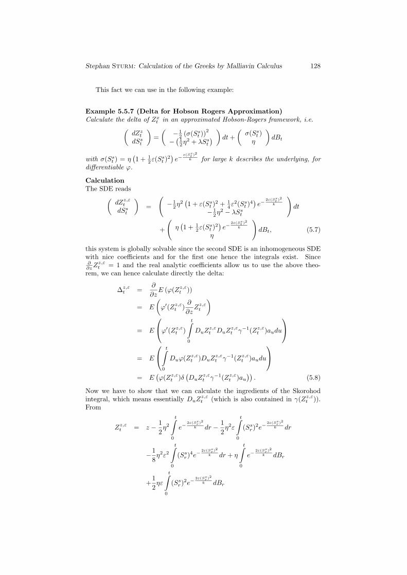
Stephan Sturm: Calculation of the Greeks by Malliavin Calculus 128
This fact we can use in the following example:
Example 5.5.7 (Delta for Hobson Rogers Approximation)Calculate the delta of Zxt in an approximated Hobson-Rogers framework, i.e.(
dZztdSst
)=(
− 12 (σ(Sst ))
2
−(
12η
2 + λSst) ) dt+
(σ(Sst )η
)dBt
with σ(Sst ) = η(1 + 1
2ε(Sst )
2)e−
ε(Sst )2
k for large k describes the underlying, fordifferentiable ϕ.
CalculationThe SDE reads(
dZz,εtdSst
)=
(− 1
2η2(1 + ε(Sst )
2 + 14ε
2(Sst )4)e−
2ε(Sst )2
k
− 12η
2 − λSst
)dt
+
(η(1 + 1
2ε(Sst )
2)e−
2ε(Sst )2
k
η
)dBt, (5.7)
this system is globally solvable since the second SDE is an inhomogeneous SDEwith nice coefficients and for the first one hence the integrals exist. Since∂∂zZ
z,εt = 1 and the real analytic coefficients allow us to use the above theo-
rem, we can hence calculate directly the delta:
∆z,εt =
∂
∂zE (ϕ(Zz,εt ))
= E
(ϕ′(Zz,εt )
∂
∂zZz,εt
)
= E
ϕ′(Zz,εt )
t∫0
DuZz,εt DuZ
z,εt γ−1(Zz,εt )audu
= E
t∫0
Duϕ(Zz,εt )DuZz,εt γ−1(Zz,εt )audu
= E
(ϕ(Zz,εt )δ
(DuZ
z,εt γ−1(Zz,εt )au
)). (5.8)
Now we have to show that we can calculate the ingredients of the Skorohodintegral, which means essentially DuZ
z,εt (which is also contained in γ(Zz,εt )).
From
Zz,εt = z − 12η2
t∫0
e−2ε(Ss
r)2
k dr − 12η2ε
t∫0
(Ssr)2e−
2ε(Ssr)2
k dr
−18η2ε2
t∫0
(Ssr)4e−
2ε(Ssr)2
k dr + η
t∫0
e−2ε(Ss
r)2
k dBr
+12ηε
t∫0
(Ssr)2e−
2ε(Ssr)2
k dBr
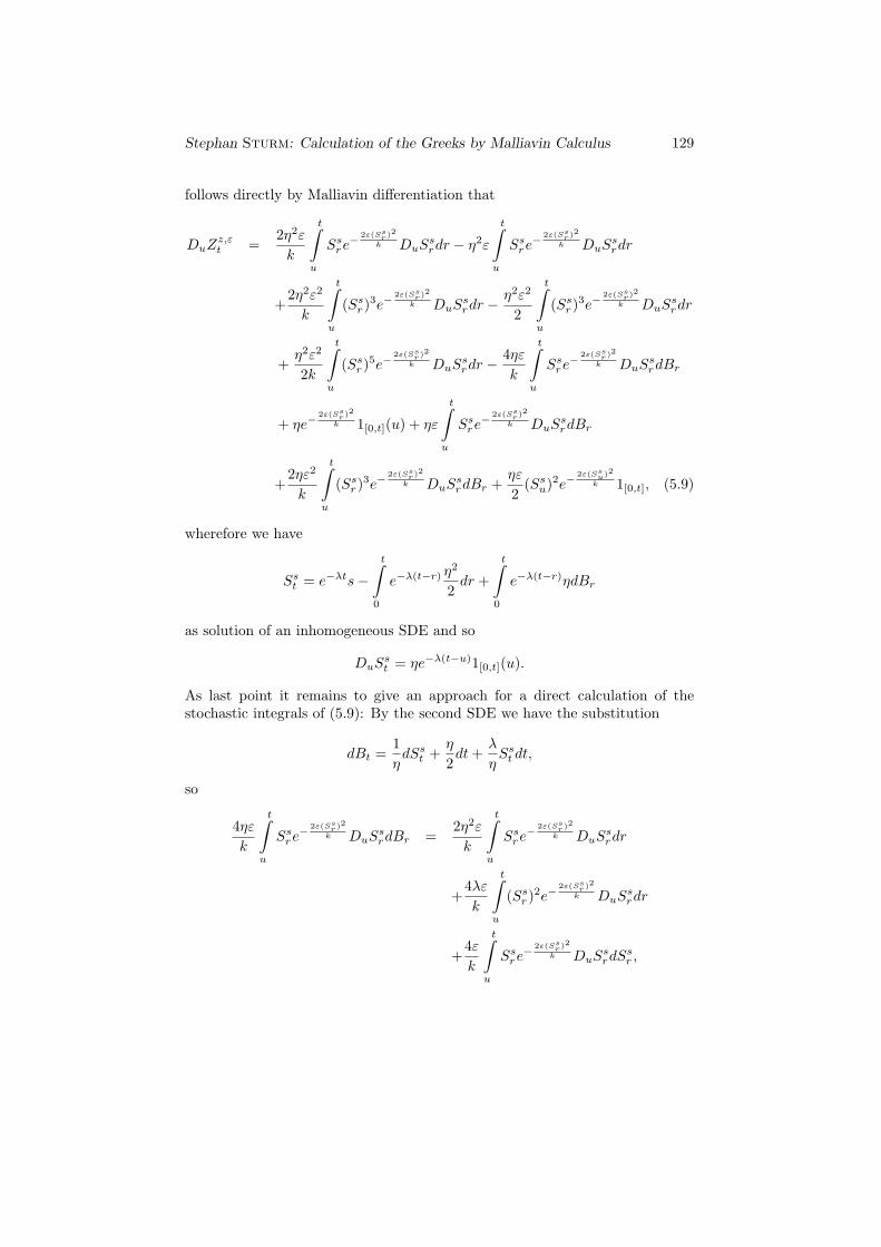
Stephan Sturm: Calculation of the Greeks by Malliavin Calculus 129
follows directly by Malliavin differentiation that
DuZz,εt =
2η2ε
k
t∫u
Ssre− 2ε(Ss
r)2
k DuSsrdr − η2ε
t∫u
Ssre− 2ε(Ss
r)2
k DuSsrdr
+2η2ε2
k
t∫u
(Ssr)3e−
2ε(Ssr)2
k DuSsrdr −
η2ε2
2
t∫u
(Ssr)3e−
2ε(Ssr)2
k DuSsrdr
+η2ε2
2k
t∫u
(Ssr)5e−
2ε(Ssr)2
k DuSsrdr −
4ηεk
t∫u
Ssre− 2ε(Ss
r)2
k DuSsrdBr
+ ηe−2ε(Ss
r)2
k 1[0,t](u) + ηε
t∫u
Ssre− 2ε(Ss
r)2
k DuSsrdBr
+2ηε2
k
t∫u
(Ssr)3e−
2ε(Ssr)2
k DuSsrdBr +
ηε
2(Ssu)
2e−2ε(Ss
u)2
k 1[0,t], (5.9)
wherefore we have
Sst = e−λts−t∫
0
e−λ(t−r) η2
2dr +
t∫0
e−λ(t−r)ηdBr
as solution of an inhomogeneous SDE and so
DuSst = ηe−λ(t−u)1[0,t](u).
As last point it remains to give an approach for a direct calculation of thestochastic integrals of (5.9): By the second SDE we have the substitution
dBt =1ηdSst +
η
2dt+
λ
ηSst dt,
so
4ηεk
t∫u
Ssre− 2ε(Ss
r)2
k DuSsrdBr =
2η2ε
k
t∫u
Ssre− 2ε(Ss
r)2
k DuSsrdr
+4λεk
t∫u
(Ssr)2e−
2ε(Ssr)2
k DuSsrdr
+4εk
t∫u
Ssre− 2ε(Ss
r)2
k DuSsrdS
sr ,
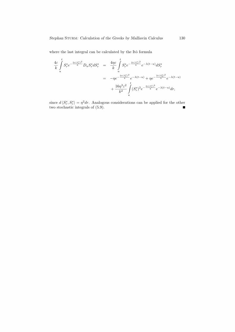
Stephan Sturm: Calculation of the Greeks by Malliavin Calculus 130
where the last integral can be calculated by the Ito formula
4εk
t∫u
Ssre− 2ε(Ss
r)2
k DuSsrdS
sr =
4ηεk
t∫u
Ssre− 2ε(Ss
r)2
k e−λ(t−u)dSsr
= −ηe−2ε(Ss
t )2
k e−λ(t−u) + ηe−2ε(Ss
0)2
k e−λ(t−u)
+16η3ε2
k2
t∫u
(Ssr)2e−
2ε(Ssr)2
k e−λ(t−u)dr,
since d 〈Ssr , Ssr〉 = η2dr. Analogous considerations can be applied for the othertwo stochastic integrals of (5.9).
Stephan Sturm: Calculation of the Greeks by Malliavin Calculus 131
Bibliography
[Ba 95] Bass, Richard F. Probabilistic Techniques in Analysis. New York(Springer) 1995
[Ba 98] Bass, Richard F. Diffusions and Elliptic Operators. New York(Springer) 1998
[Bor 95] Borkar, Vivek S. Probability Theory. An Advanced Course. NewYork (Springer) 1995
[ChW 83] Chung, Kai Lai and Williams, Ruth J. Introduction to Stochas-tic Integration. Boston (Birkhauser) 1983
[DM 78] Dellacherie, Claude and Meyer, Paul-Andre. Probabilitiesand Potential (Chapter 0 - IV). Paris (Hermann) and Amsterdam (North Hol-land) 1978
[DM 80] Dellacherie, Claude and Meyer, Paul-Andre. Probabilites etPotentiel (Chapitre V - VIII). Paris (Hermann) 1980
[Eth 02] Etheridge, Alison. Financial Calculus. Cambridge (CambridgeUniversity Press) 2002
[FLLLT 99] Fournie, Eric, Lasry, Jean-Michel, Lebuchoux, Jerome,Lions, Pierre-Louis and Touzi, Nizar. Application of Malliavin calculus toMonte Carlo methods in finance. Finance and Stochastics, 3 (1999), 391-412
[FLLL 01] Fournie, Eric, Lasry, Jean-Michel, Lebuchoux, Jerome andLions, Pierre-Louis. Application of Malliavin calculus to Monte Carlo methodsin finance. II. Finance and Stochastics, 5 (2001), 201-236
[GM 02] Gobet, Emmanuel and Munos, Remi. Sensitivity Analysis us-ing Ito-Malliavin Calculus and Martingales. Application to Stochastic OptimalControl. 2002 (preprint)
[Ho 83] Hormander, Lars. The Analysis of Partial Differential OperatorsI. Distribution Theory and Fourier Analysis. Berlin (Springer) 1983
[HTT] Hubalek, Friedrich, Teichmann, Josef and Tompkins, Robert.Flexible Complete Models with Stochastic Volatility Generalising Hobson &Rogers. 2003 (working paper)
[Im 97] Imkeller, Peter. Der stochastische Variationskalkul und Anwen-dungen in der multiplikativen Ergodentheorie. Manuscript. 1997(http://wws.mathematik.hu-berlin.de/˜imkeller/teaching lectures/Supplement/buckow.pdf)
[Kal 02] Kallenberg, Olav. Foundations of Modern Probability. NewYork (Springer) 22002
Stephan Sturm: Calculation of the Greeks by Malliavin Calculus 132
[KS 88] Karatzas, Ioannis and Shreve, Steven E. Brownian Motion andStochastic Calculus. New York (Springer) 1988
[Mal 95] Malliavin, Paul e.a. Integration and Probability. New York(Springer) 1995
[Mi 97] Michor, Peter W. Transformation Groups. Lecture Notes of acourse in Vienna. 1997 (http://www.mat.univie.ac.at/˜michor/tgbook.ps)
[MT 03] Malliavin, Paul and Thalmaier, Anton. Stochastic Calculusof Variations in Mathematical Finance. Preliminary draft of the first chapters.Berlin (Springer) 2003 (preprint)
[Nua 95] Nualart, David. The Malliavin Calculus and Related Topics.New York (Springer) 1995
[Øks 85] Øksendal, Bernt Karsten. Stochastic Differential Equations. AnIntroduction with Applications. Berlin (Springer) 1985
[Øks 97] Øksendal, Bernt. An Introduction to Malliavin Calculus withApplications to Economics. Manuscript. Oslo 1997(http://www.nhh.no/for/dp/1996/wp0396.pdf)
[Rud 87] Rudin, Walter. Real and Complex Analysis. New York (McGraw-Hill) 31987
[Rud 91] Rudin, Walter. Functional Analysis. New York (McGraw-Hill)21991
[RY 91] Revuz, Daniel and Yor, Marc. Continuous Martingales and Brow-nian Motion. Berlin (Springer) 1991
[Sch 99] Schaefer, H.H. with Wolff, M.P. Topological Vector Spaces.New York (Springer) 21999
[Tei 02] Teichmann, Josef. The Malliavin Calculus. Manuscript. Vienna2002 (http://www.fam.tuwien.ac.at/˜jteichma/lecture.html)
[Tei 03] Teichmann, Josef. Stochastic Analysis with Applications to Fi-nancial and Actuarial Mathematics. Manuscript. Vienna 2003(http://www.fam.tuwien.ac.at/˜jteichma/lecture.html)
[TT] Teichmann, Josef and Touzi, Nizar. Calculating the Greeks for hy-poelliptic Problems. (working paper)
[Wat 84] Watanabe, S. Stochastic Differential Equations and MalliavinCalculus. Bombay (Tata Institute of Fundamental Research) and Berlin (Springer)1984
Contents
1 Preliminaries 51.1 Stochastic Processes and Martingales . . . . . . . . . . . . . . . . 5
1.1.1 Stochastic Processes . . . . . . . . . . . . . . . . . . . . . 51.1.2 Martingales . . . . . . . . . . . . . . . . . . . . . . . . . . 8
1.2 Tensor Products . . . . . . . . . . . . . . . . . . . . . . . . . . . 14
2 Brownian Motion and Stochastic Integration 162.1 Gaussian Processes . . . . . . . . . . . . . . . . . . . . . . . . . . 192.2 Brownian Motion . . . . . . . . . . . . . . . . . . . . . . . . . . . 202.3 Ito Integration . . . . . . . . . . . . . . . . . . . . . . . . . . . . 232.4 Generalizing the Ito Integral: Integration along Continuous Semi-
martingales . . . . . . . . . . . . . . . . . . . . . . . . . . . . . . 322.4.1 Martingales and Quadratic Variation . . . . . . . . . . . . 332.4.2 Stochastic Integrals with respect to
Continuous Semimartingales . . . . . . . . . . . . . . . . 432.4.3 Ito’s Formula . . . . . . . . . . . . . . . . . . . . . . . . . 462.4.4 The Stratonovich Integral . . . . . . . . . . . . . . . . . . 49
2.5 Transformations of the Probability Measure . . . . . . . . . . . . 51
3 Stochastic Differential Equations 583.1 Some Inequalities . . . . . . . . . . . . . . . . . . . . . . . . . . . 583.2 Solutions of SDEs . . . . . . . . . . . . . . . . . . . . . . . . . . 643.3 Flows and the First Variation . . . . . . . . . . . . . . . . . . . . 69
4 Wiener Chaos and Malliavin Derivatives 784.1 The Wiener Chaos Decomposition . . . . . . . . . . . . . . . . . 78
4.1.1 Hermite Polynomials . . . . . . . . . . . . . . . . . . . . . 784.1.2 Wiener Chaos . . . . . . . . . . . . . . . . . . . . . . . . . 82
4.2 Multiple Wiener-Ito Integrals . . . . . . . . . . . . . . . . . . . . 854.2.1 Multiple Wiener-Ito Integrals . . . . . . . . . . . . . . . . 864.2.2 Wiener-Ito Integrals as Stochastic Integrals . . . . . . . . 89
4.3 Malliavin Derivatives . . . . . . . . . . . . . . . . . . . . . . . . . 914.4 The Skorohod Integral . . . . . . . . . . . . . . . . . . . . . . . . 1004.5 Malliavin Derivative and First Variation . . . . . . . . . . . . . . 107
133
Stephan Sturm: Calculation of the Greeks by Malliavin Calculus 134
5 Calculating the Greeks 1115.1 Pricing Options: A very rough Primer . . . . . . . . . . . . . . . 1115.2 The Greeks . . . . . . . . . . . . . . . . . . . . . . . . . . . . . . 1125.3 The Elliptic Case . . . . . . . . . . . . . . . . . . . . . . . . . . . 114
5.3.1 The Rho . . . . . . . . . . . . . . . . . . . . . . . . . . . . 1145.3.2 The Delta . . . . . . . . . . . . . . . . . . . . . . . . . . . 1165.3.3 The Vega . . . . . . . . . . . . . . . . . . . . . . . . . . . 118
5.4 Beyond Ellipticity . . . . . . . . . . . . . . . . . . . . . . . . . . 1215.5 Examples . . . . . . . . . . . . . . . . . . . . . . . . . . . . . . . 124
![Malliavin Calculus MethodforAsymptotic … · Malliavin calculus has found applications in other areas of mathematical finance, such 20], to computation of sensitivity parameters](https://img.pdfslide.net/doc/110x75/604d8e0a0789235d9d4ffc7f/malliavin-calculus-methodforasymptotic-malliavin-calculus-has-found-applications.jpg)


![[B][i]Grasselli{Matheus}Hurd{Tom}-Malliavin Calculus](https://img.pdfslide.net/doc/110x75/577d1ec11a28ab4e1e8f2cf1/bigrassellimatheushurdtom-malliavin-calculus.jpg)


![[Oksendal B.] Introductiont to Malliavin Calculus (BookFi.org)](https://img.pdfslide.net/doc/110x75/55cf9d6a550346d033ad8405/oksendal-b-introductiont-to-malliavin-calculus-bookfiorg.jpg)