Embed Size (px)
Citation preview
CAN UNCLASSIFIED
Calculation software for ballistic limit and Vproof tests from ballistic tests results (BLC)
Daniel Bourget Manon Bolduc DRDC – Valcartier Research Centre
The body of this CAN UNCLASSIFIED document does not contain the required security banners according to DND security standards. However, it must be treated as CAN UNCLASSIFIED and protected appropriately based on the terms and conditions specified on the covering page.
CAN UNCLASSIFIED
July 2020
DRDC-RDDC-2020-R056
Scientific Report
Defence Research and Development Canada

CAN UNCLASSIFIED
Template in use: EO Publishing App for SR-RD-EC Eng 2018-12-19_v1 (new disclaimer).dotm © Her Majesty the Queen in Right of Canada (Department of National Defence), 2020
© Sa Majesté la Reine en droit du Canada (Ministère de la Défense nationale), 2020
CAN UNCLASSIFIED
IMPORTANT INFORMATIVE STATEMENTS
This document was reviewed for Controlled Goods by Defence Research and Development Canada (DRDC) using the Schedule to the Defence Production Act.
Disclaimer: This publication was prepared by Defence Research and Development Canada an agency of the Department of National Defence. The information contained in this publication has been derived and determined through best practice and adherence to the highest standards of responsible conduct of scientific research. This information is intended for the use of the Department of National Defence, the Canadian Armed Forces (“Canada”) and Public Safety partners and, as permitted, may be shared with academia, industry, Canada’s allies, and the public (“Third Parties”). Any use by, or any reliance on or decisions made based on this publication by Third Parties, are done at their own risk and responsibility. Canada does not assume any liability for any damages or losses which may arise from any use of, or reliance on, the publication.
Endorsement statement: This publication has been peer-reviewed and published by the Editorial Office of Defence Research and Development Canada, an agency of the Department of National Defence of Canada. Inquiries can be sent to: [email protected].
DRDC-RDDC-2020-R056 i
Abstract
This document provides scientific information on the mathematical and statistical methods used by the
BLC (Ballictic Limit Calculator) Beta Version 2 program to generate ballistic limit and Vproof data and
their related statistics based on experimental ballistic data.
The BLC software enables the analysis of ballistic data using 5 different statistical models (namely, the
Probit, Logit, Gompit, Scobit and Weibull models) that, at least for the Probit and Logit models, follow
the data analysis procedures of NATO STANAG 2920 and NIJ 0101.06 standards. In addition to the
model parameters, BLC calculates standard errors and confidence limits on the model parameters, on the
ballistic limit, on the standard deviation and on the Vproof. Furthermore, a series of statistical tests
enables the comparison of the different models and allows to assess their significance and goodness of fit.
This document is also the user manual of the BLC Beta version 2 program. As such, this document
provides details on the nature and meaning of input and output information and presents its different
features.
Significance to defence and security
This document describes the use and scientific foundation of the Ballistic Limit Calculator (BLC)
software. The BLC provides straightforward statistical analysis of raw ballistic data to determine the
protection level provided by armour against specific projectiles.
ii DRDC-RDDC-2020-R056
Résumé
Ce document fournit des informations scientifiques sur les méthodes mathématiques et statistiques
utilisées par le programme BLC (Ballictic Limit Calculator) Beta Version 2 pour générer des données de
limite balistique et Vproof et leurs statistiques associées basées sur des données balistiques
expérimentales.
Le logiciel BLC permet l'analyse de données balistiques à l'aide de 5 modèles statistiques différents (à
savoir, les modèles Probit, Logit, Gompit, Scobit et Weibull) qui, au moins pour les modèles Probit et
Logit, suivent les procédures d'analyse des données des normes OTAN STANAG 2920 et NIJ 0101.06
STANAG 2920 et NIJ Normes 0101.06. En plus des paramètres du modèle, BLC calcule les erreurs
standards et les limites de confiance sur les paramètres du modèle, sur la limite balistique, sur l'écart type
et sur le Vproof. En outre, une série de tests statistiques permet la comparaison des différents modèles et
permet d'évaluer leur signification et leur qualité d'ajustement.
Ce document est également le manuel d'utilisation du programme BLC Beta version 2. À ce titre, ce
document fournit des détails sur la nature et la signification des informations d'entrée et de sortie et
présente ses différentes caractéristiques.
Importance pour la défense et la sécurité
Ce document décrit l'utilisation et les fondements scientifiques du logiciel Ballistic Limit
Calculator (BLC). Le BLC fournit une analyse statistique simple des données balistiques brutes
pour déterminer le niveau de protection fourni par l'armure contre des projectiles spécifiques.
DRDC-RDDC-2020-R056 iii
Table of contents
Abstract . . . . . . . . . . . . . . . . . . . . . . . . . . . . . . . . . . . i
Significance to defence and security . . . . . . . . . . . . . . . . . . . . . . . . . i
Résumé . . . . . . . . . . . . . . . . . . . . . . . . . . . . . . . . . . . ii
Importance pour la défense et la sécurité . . . . . . . . . . . . . . . . . . . . . . . ii
Table of contents . . . . . . . . . . . . . . . . . . . . . . . . . . . . . . . iii
List of figures . . . . . . . . . . . . . . . . . . . . . . . . . . . . . . . . . v
List of tables . . . . . . . . . . . . . . . . . . . . . . . . . . . . . . . . . vi
1 Introduction . . . . . . . . . . . . . . . . . . . . . . . . . . . . . . . . 1
1.1 General . . . . . . . . . . . . . . . . . . . . . . . . . . . . . . . . 1
1.2 Ballistic tests for which this software can be used . . . . . . . . . . . . . . . . 1
2 User manual . . . . . . . . . . . . . . . . . . . . . . . . . . . . . . . . 3
2.1 How to use the BLC . . . . . . . . . . . . . . . . . . . . . . . . . . . 3
2.2 Execution warnings . . . . . . . . . . . . . . . . . . . . . . . . . . . 6
2.3 Execution errors . . . . . . . . . . . . . . . . . . . . . . . . . . . . . 7
3 Ballistic limit calculation procedures . . . . . . . . . . . . . . . . . . . . . . . 8
3.1 General . . . . . . . . . . . . . . . . . . . . . . . . . . . . . . . . 8
3.2 Link Functions . . . . . . . . . . . . . . . . . . . . . . . . . . . . . 8
3.2.1 Probit . . . . . . . . . . . . . . . . . . . . . . . . . . . . . . 8
3.2.2 Logit . . . . . . . . . . . . . . . . . . . . . . . . . . . . . . 9
3.2.3 Gompit . . . . . . . . . . . . . . . . . . . . . . . . . . . . . 9
3.2.4 Scobit . . . . . . . . . . . . . . . . . . . . . . . . . . . . . . 9
3.2.5 Weibull . . . . . . . . . . . . . . . . . . . . . . . . . . . . . 9
3.2.6 Summary of link functions . . . . . . . . . . . . . . . . . . . . . 10
3.3 Fitting Process Calculations . . . . . . . . . . . . . . . . . . . . . . . 11
3.3.1 General . . . . . . . . . . . . . . . . . . . . . . . . . . . . 11
3.3.2 Maximum Likelihood Estimation (ML) . . . . . . . . . . . . . . . . 12
3.4 Confidence Interval and Standard Error Calculation . . . . . . . . . . . . . . 13
3.4.1 General . . . . . . . . . . . . . . . . . . . . . . . . . . . . 13
3.4.2 Standard Error Estimation . . . . . . . . . . . . . . . . . . . . . 13
3.4.3 Confidence interval curves . . . . . . . . . . . . . . . . . . . . . 14
3.4.3.1 Normal error distribution confidence interval . . . . . . . . . . . 14
3.4.3.2 Binomial error distribution confidence interval . . . . . . . . . . 15
4 Diagnostic tools . . . . . . . . . . . . . . . . . . . . . . . . . . . . . . 17
4.1 General . . . . . . . . . . . . . . . . . . . . . . . . . . . . . . . 17
4.2 Information on the data sample . . . . . . . . . . . . . . . . . . . . . . 17
4.2.1 Sample Statistics section of the “Results 1” sheet . . . . . . . . . . . . . 17
4.2.2 Box Plot sheet. . . . . . . . . . . . . . . . . . . . . . . . . . 18

iv DRDC-RDDC-2020-R056
4.3 Tests on validity of the data . . . . . . . . . . . . . . . . . . . . . . . 19
4.3.1 Criteria for validity of dependent variable value independency . . . . . . . . 20
4.3.1.1 MONOBIT Test . . . . . . . . . . . . . . . . . . . . . 20
4.3.1.2 RUNS Test . . . . . . . . . . . . . . . . . . . . . . . 21
4.3.1.3 Cumulative Sum Test . . . . . . . . . . . . . . . . . . . 21
4.4 The Goodness-of-Fit and Significance of the model . . . . . . . . . . . . . . 22
4.4.1 Significance of the parameters and independent variables . . . . . . . . . . 22
4.4.1.1 Likelihood Ratio Test . . . . . . . . . . . . . . . . . . . 22
4.4.1.2 Wald Test . . . . . . . . . . . . . . . . . . . . . . . . 23
4.4.2 Goodness-of-Fit Tests . . . . . . . . . . . . . . . . . . . . . . . 24
4.4.2.1 Anderson-Darling Test . . . . . . . . . . . . . . . . . . . 24
4.4.2.2 Sensitivity, Specificity and area under the ROC curve (AUC) . . . . . 26
4.4.2.3 The Stukel Test . . . . . . . . . . . . . . . . . . . . . . 28
4.4.2.4 Pseudo-R2 . . . . . . . . . . . . . . . . . . . . . . . . 28
4.4.2.5 Information Criterion (IC): General considerations. . . . . . . . . 29
4.4.2.6 The small sample size corrected AIC . . . . . . . . . . . . . . 31
4.4.2.7 Small sample size correction using the Bootstrap method (EIC) . . . . 31
5 Results description . . . . . . . . . . . . . . . . . . . . . . . . . . . . . 33
5.1 Summary data (“Results 1” sheet) . . . . . . . . . . . . . . . . . . . . . 33
5.1.1 Experimental data sample statistics . . . . . . . . . . . . . . . . . . 33
5.1.2 Independency of dependent variable . . . . . . . . . . . . . . . . . 33
5.1.3 Parameter values and statistics. . . . . . . . . . . . . . . . . . . . 34
5.1.4 Significance of the model . . . . . . . . . . . . . . . . . . . . . 34
5.1.5 Goodness-of-fit of the model . . . . . . . . . . . . . . . . . . . . 35
5.1.6 Data analysis based on STANAG 2920 . . . . . . . . . . . . . . . . 36
5.1.7 Confidence Interval at V50 based on Normal of Binomial error distribution . . . 37
5.1.8 Vproof statistics . . . . . . . . . . . . . . . . . . . . . . . . . 38
5.2 Experimental data points and confidence limit curves (“Results 2” sheet) . . . . . . 39
5.3 Other sheets . . . . . . . . . . . . . . . . . . . . . . . . . . . . . 39
5.3.1 Box Plot sheet. . . . . . . . . . . . . . . . . . . . . . . . . . 39
5.3.2 Proofing Statistics sheet . . . . . . . . . . . . . . . . . . . . . . 40
5.3.3 Graphical output sheets . . . . . . . . . . . . . . . . . . . . . . 41
5.3.4 ROC sheet . . . . . . . . . . . . . . . . . . . . . . . . . . . 41
6 Data analysis example . . . . . . . . . . . . . . . . . . . . . . . . . . . . 42
6.1 General . . . . . . . . . . . . . . . . . . . . . . . . . . . . . . . 42
6.2 Determination of the correct model . . . . . . . . . . . . . . . . . . . . . 42
6.2.1 Guidelines . . . . . . . . . . . . . . . . . . . . . . . . . . . 42
6.2.2 Correct model determination: An example . . . . . . . . . . . . . . . 44
6.3 Ballistic limit and Vproof analysis . . . . . . . . . . . . . . . . . . . . . 46
7 Conclusion . . . . . . . . . . . . . . . . . . . . . . . . . . . . . . . . 48
References . . . . . . . . . . . . . . . . . . . . . . . . . . . . . . . . . 49
DRDC-RDDC-2020-R056
List of figures
Figure 1: The “Main” sheet. ................................................................................................................. 3
Figure 2: The “Navigation Menu”. ...................................................................................................... 4
Figure 3: Screen during code execution. .............................................................................................. 5
Figure 4: Density probability (left) and cumulative probability (right) distribution curves for the
Probit, Logit, Gompit, Scobit and Weibull distributions. For the Scobit and the Weibull
distributions, curves for 2 different shape parameter values are shown
(δ = 0.5 and δ = 2.0). ........................................................................................................... 10
Figure 5: Box plot of a symmetric sample distribution (left side, calculated skewness = -0.19)
and a positively-skewed sample distribution (right side, calculated skewness = +1.51). ... 19
Figure 6: Example of an ROC curve. ................................................................................................. 26
Figure 7: Illustration of V50 statistics. In this example, STANAG 2920 maximal and minimal
V50 values are located within the normal error distribution bracket. It is not necessary
always the case. .................................................................................................................. 37
Figure 8: Schematic illustrating Vproof statistics with an example for 10% probability of
perforation. The fitted cumulative function is presented in red, the lower confidence
limit is presented in purple and the upper confidence limit is presented in green. ............ 39
Figure 9: Example of perforation probability fitted curve for normal error (left) and binomial
error (right) distribution for 95% confidence level. ............................................................ 41
Figure 10: Decision process to determine best model. ......................................................................... 44
Figure 11: Curve fit statistics data for the Logit, Probit and Scobit models. ....................................... 46
v
DRDC-RDDC-2020-R056
List of tables
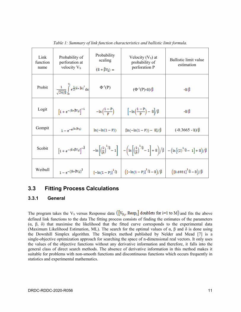
Table 1: Summary of link function characteristics and ballistic limit formula. . . . . . . . 11
Table 2: List of assumptions for OLS versus GLM fitting process. . . . . . . . . . . . . 19
Table 3: Power level of the AD test for normality for symmetric and asymmetric distributions
with varying skewness (Sk), kurtosis (Ku), Type I error level (α) and number of data
points in the distribution (n). Data from [28]. . . . . . . . . . . . . . . . . . 25
Table 4: Classification table for a predetermined threshold value. . . . . . . . . . . . . 27
Table 5: – ROC AUC qualitative level of discrimination . . . . . . . . . . . . . . . . 35
Table 6: Example of the number of perforation allowed (Allowed Nb of failure) and total
number of shots to fire (Nb of shot required) to test 10% probability of perforation
(V10%) with a confidence level of 95% (CL = 95%). . . . . . . . . . . . . . . 40
Table 7: Variables of interest for Ballistic Limit and Vproof data analysis in “Result 1”
Worksheet. . . . . . . . . . . . . . . . . . . . . . . . . . . . . . . 46
vi
DRDC-RDDC-2020-R056 1
1 Introduction
1.1 General
Armour is an integral part of Personal Protective Ensemble (PPE) provided to soldiers and Law
Enforcement personnel. Because they are live saving devices their performance is strictly controlled by
standards and test procedures. Different national and international bodies are managing standards (e.g.,
NATO [1][2], National Institute of Justice, NIJ [3]). Because armour material and capabilities are
evolving as well as our understanding of their interaction with the human subject wearing it, standards are
continually evolving. One recent evolution concerns the number of ballistic impacts used to assess
ballistic limit performance of armours and the use of ballistic data fitting techniques to model the
probability of perforation. In addition, requirements to specify confidence intervals for safe protection
impact velocity value (Vproof) have appeared in different NATO standards. Due to the extensive
mathematical process related to these new ways of assessing armour performance and new requirements,
an Microsoft Excel ballistic data analysis package calle BLC (Ballistic Limit Calculator) was created.
This document provides scientific information on the mathematical and statistical methods used by the
BLC Beta version 2 program to generate ballistic limit and Vproof data and their related statistics based
on experimental ballistic data. This document is also the user manual of the BLC Beta version 2 program.
Therefore, this document addresses the needs of technicians, engineers and scientists on the capability,
procedures, scientific background, usage and caveats of BLC with the goal of providing enlightened
assessment of armour performance.
1.2 Ballistic tests for which this software can be used
The MS Excel “BLC Beta version 2.xls” file can be used to calculate the ballistic limit value and the
Vproof statistics based on experimental ballistic data. These two tests are the most common ballistic
control tests.
Ballistic limit (V50) tests: Ballistic limit is the velocity at which the probability of perforation of an
armour is 50% That velocity is calculated, using statistical procedure, for a specific armour and a
specific threat. The ballistic limit is often used during armour production for controlling the
performance variability between batches (combination of material and manufacturing variabilities)
and maintaining the quality of the armour material. The ballistic limit is calculated based on a series
of shots fired at an armour following a pre-defined impact pattern for a range of impact velocity
above and below the V50 value for which perforation (1) or non-perforation (0) are recorded. The
sequence of impact velocity follows an up and down procedure described in STANAG 2920 ([1],
[2]) and NIJ 0101.06 [3]. The ballistic limit can also be considered as the upper limit of protection
where the probability of perforation is 50% in comparison to the Vproof test where the probability
of perforation is lower.
Vproof tests: It is also called a ballistic resistance tests. The Vproof is a PASS/FAIL test for which
a certain number of shot is fired at a fixed velocity and for which a certain number of penetration
through the armour is allowed. These two values are determined depending on the probability of
perforation (e.g., 5%) for which the test needs to be done and for the confidence level (e.g., 95%)

2 DRDC-RDDC-2020-R056
that the probability of perforation is real. In BLC, Vproof statistics are calculated based on the
perforation/no perforation test results of ballistic limit tests.
DRDC-RDDC-2020-R056 3
2 User manual
2.1 How to use the BLC
To use BLC Beta version 2.xls, do the following steps:
1. Load the BLC Beta version 2.xls file into Excel by double clicking on the file icon.
2. Once loaded, the program displays the “Main” page where inputs can be entered and a floating
“Navigation Menu”on top of it. The “Navigation Menu” cannot be closed, but it can be minimized
and placed anywhere on the screen for further recall.
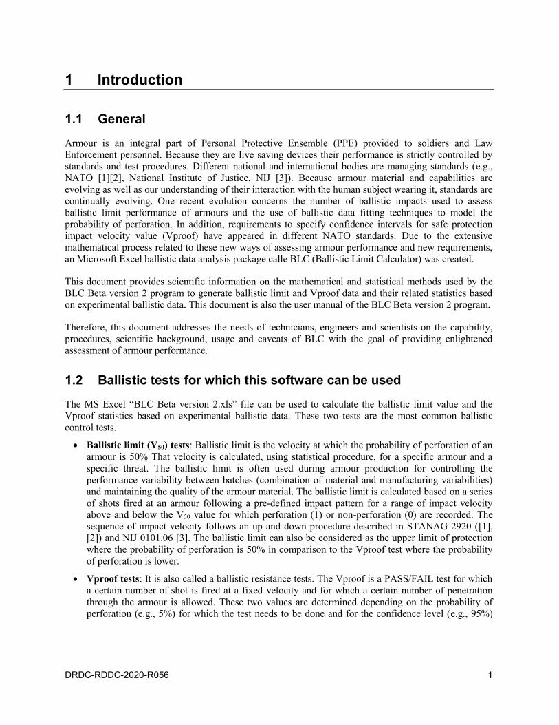
3. Following is a description of the “Main” sheet and “Navigation Menu” features
Figure 1: The “Main” sheet.
a. The “Main” sheet (Figure 1):
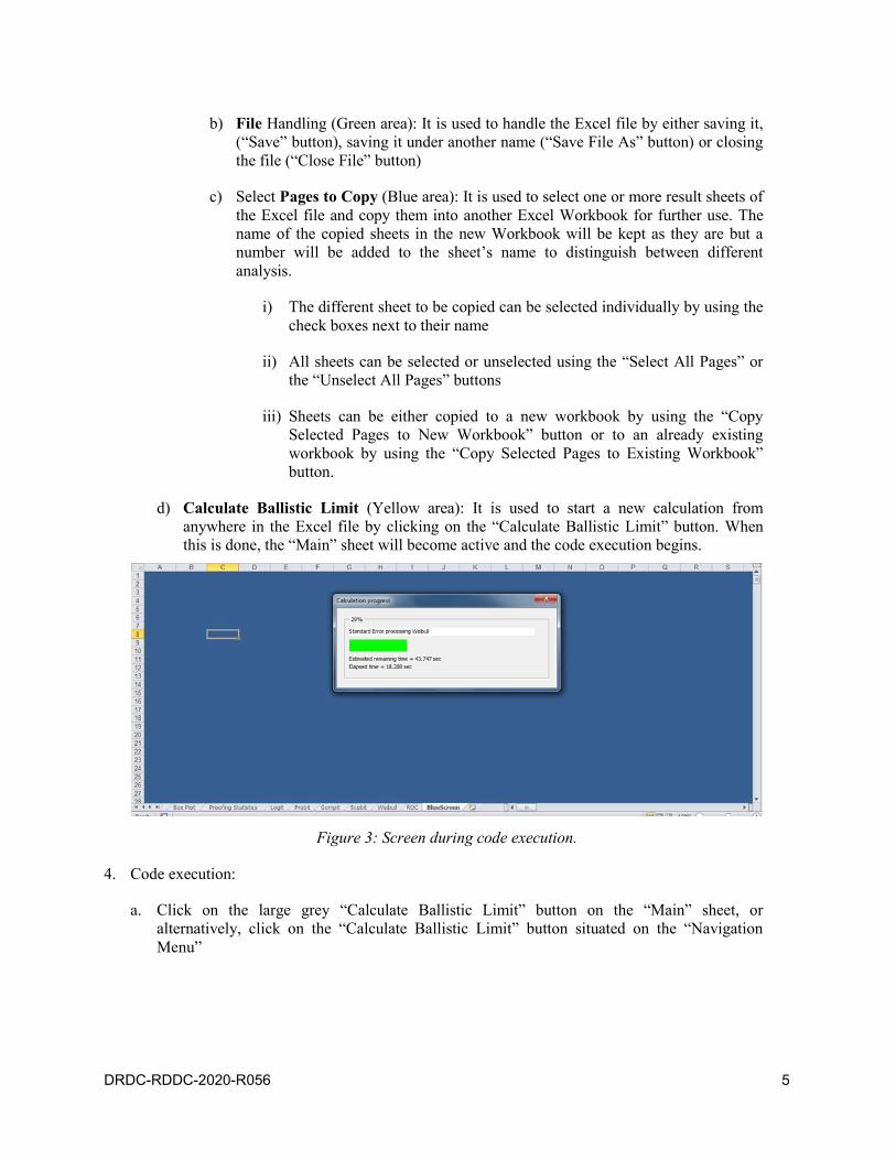
i. In the “Main” sheet, enter your experimental ballistic data in the order in which they
were fired (see Section 4.3.1):
a) Column A: Striking velocities (VS).
b) Column B: Response. For a complete perforation of the target, the value entered
can be either 1, “Y”, “y” or “CP”. For a partial perforation, the value entered can
be either 0, “N”, “n” or “PP”.
c) Column C: Wether or not you want the data be used in the ballistic limit and
Vproof calculation. If you want to use the data point, enter a 1. If you do not
want to use the data point, enter 0. This feature was added to allow flexibility for
removing or adding data points.
4 DRDC-RDDC-2020-R056
d) It is possible to enter up to 500 data points. Copy/paste can be used to insert data
in the different columns
ii. Select the Error distribution shape. For this version of the software, it can be either
Normal or Binomial.
iii. Select the confidence level for error distribution (value between 0.001 and 0.999) for
the V50 and Vproof confidence interval calculation.
iv. Select the Vproof probability value (value between 0.001 and 0.999). Vproof
probability is the perforation probability for which Vproof statistics are calculated by
the program.
v. Select the statistical test confidence level (value between 0.001 and 0.999), This value
will be used by the program as the threshold probability for the statistical inference
tests.
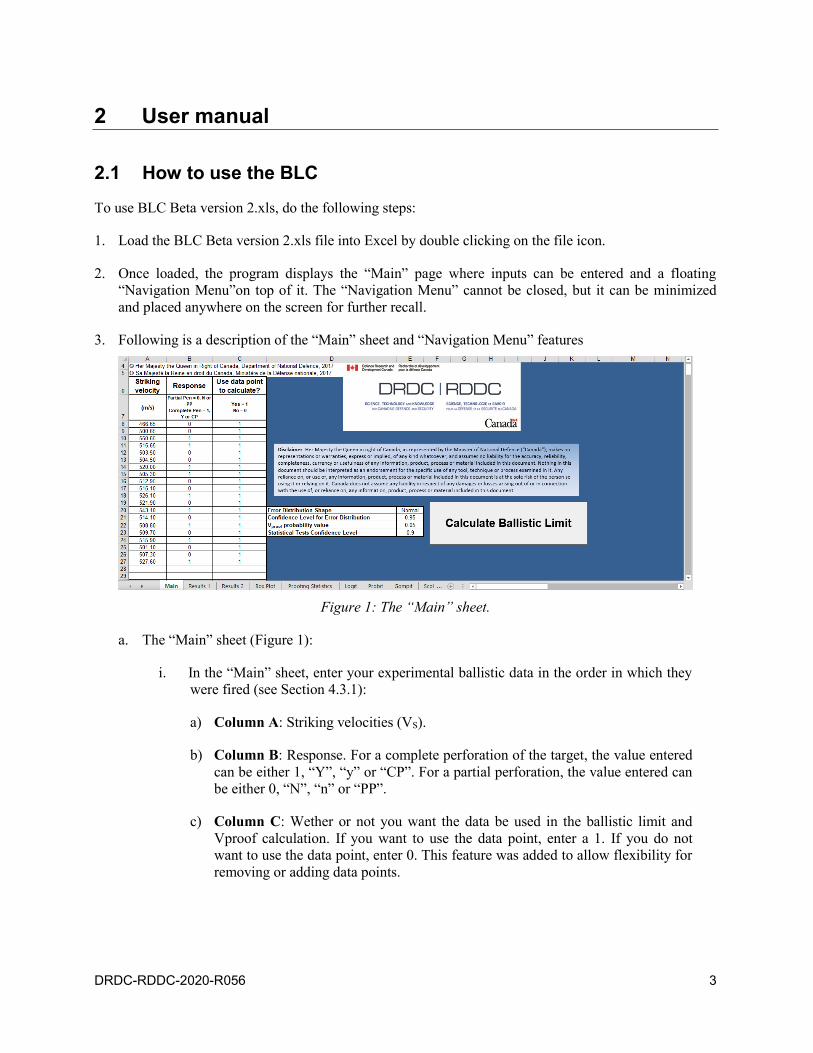
Figure 1 – The “Navigation Menu” Figure 2: The “Navigation Menu”.
b. Navigation in the software
i. It is possible to navigate in the program by using the Excel tabs located at the bottom
of the screen.
ii. It is also possible to navigate in the program by using The “Navigation Menu”
(Figure 2). It is divided as follows:
a) Navigation (Red area): It is is used to navigate from any pages in the Excel file
to the 3 most frequently used pages, that is the “Main” sheet, the “Results 1”
sheet and the “Results 2” sheet by using the respective buttons.
DRDC-RDDC-2020-R056 5
b) File Handling (Green area): It is used to handle the Excel file by either saving it,
(“Save” button), saving it under another name (“Save File As” button) or closing
the file (“Close File” button)
c) Select Pages to Copy (Blue area): It is used to select one or more result sheets of
the Excel file and copy them into another Excel Workbook for further use. The
name of the copied sheets in the new Workbook will be kept as they are but a
number will be added to the sheet’s name to distinguish between different
analysis.
i) The different sheet to be copied can be selected individually by using the
check boxes next to their name
ii) All sheets can be selected or unselected using the “Select All Pages” or
the “Unselect All Pages” buttons
iii) Sheets can be either copied to a new workbook by using the “Copy
Selected Pages to New Workbook” button or to an already existing
workbook by using the “Copy Selected Pages to Existing Workbook”
button.
d) Calculate Ballistic Limit (Yellow area): It is used to start a new calculation from
anywhere in the Excel file by clicking on the “Calculate Ballistic Limit” button. When
this is done, the “Main” sheet will become active and the code execution begins.
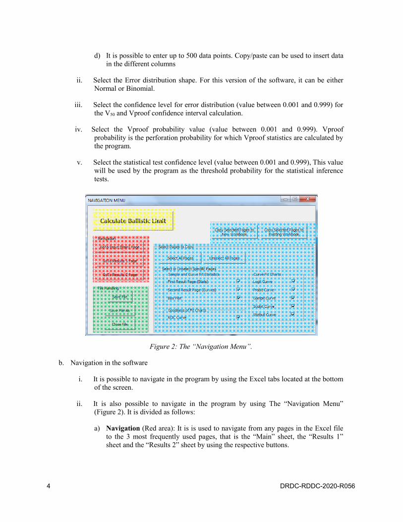
Figure 3: Screen during code execution.
4. Code execution:
a. Click on the large grey “Calculate Ballistic Limit” button on the “Main” sheet, or
alternatively, click on the “Calculate Ballistic Limit” button situated on the “Navigation
Menu”
6 DRDC-RDDC-2020-R056
b. The program will ask to select the range of cells containing the experimental data that were
entered on the “Main” sheet. Data must be selected in columns A, B and C.
c. After you have selected the range, click OK
d. If there are issues with the data, the program will display warning messages. See Section 2.2
and 2.3 on execution warnings and execution errors.
e. During execution, the program stays on a blank blue page and displays a progress bar.
(Figure 3). Be patient. A typical 12 to 25 data points analysis takes about 50 to 60 seconds. A
100 data points analysis takes about 80 seconds
f. At the end of the execution, the progress bar displays a “Done” button. Pressing enter or
clicking on the “Done” button will close the progress bar and the “Navigation Menu” will
reappear.
2.2 Execution warnings
The program may display warnings in circumstances describe below. For some warnings (Termination
Errors), the user will have to click the “Ok” button, check data on the “Main” sheet and click again on the
“Calculate Ballistic Limit” button to start the calculation again.
For some others (Warning to the User), the User can either click on the “Cancel” button in which case
he/she will check data on the “Main” sheet and click again on the “Calculate Ballistic Limit” button to
start the calculation again, or the User can click on the “Retry” button in which case the calculation
continues using the same data.
1. Termination Errors:
a. If more then three columns were selected for the VS/Response/Calculation data.
b. If less then two rows were selected for the VS/Response/Calculation data.
c. If a value of VS in the VS/Response list is less then or equal to 0.
d. If a value of Response in the VS/Response list is different from 0, “n”, “N” and “PP” or
different from 1, “y”, “Y” and “CP”.
e. If the selected values of Response contains only 0 or only 1 values.
f. If the Confidence Level for Error Distribution, the Vproof probability value or the
Statistical Tests Confidence Level values entered are not between 0 and 1 (0 and 1 excluded).
2. Warning to the User
a. If the number of partial perforation is more then 0 and less than 3
b. If the number of complete perforation is more then 0 and less than 3
DRDC-RDDC-2020-R056 7
c. If the highest VS value is not a complete perforation
d. If the lowest VS value is not a partial perforation
2.3 Execution errors
Although it has been extensively tested, the BLC software can still present errors during runtime. Usually,
when such an error occurs, a message is displayed on the screen starting with “Error in” followed by the
name of a function or a subroutine name. A “Ok” button also appears on the message. When click, the
“Ok” button will resume the code execution.
In case such errors occur, please contact the author of this document. Please also provide the error
message along with all the data that was used in the “Main” sheet.
The author’s coordinate are:
By e-mail at [email protected], or [email protected]
By phone at (001) 418-844-4000 ext 4228.

8 DRDC-RDDC-2020-R056
3 Ballistic limit calculation procedures
3.1 General
The V50 is the convergence value from the data produced by the up and down technique around the
velocity at which 50 % of shots penetrated and 50% are stopped by the armour system. The procedure to
evaluate the V50 is well described in the the STANAG 2920 (Edition 3) [1] and [2] and the NIJ 0101.06
[3]. The up and down technique is used to minimize the number of shots while finding the convergence
point. For each impact velocity, the status of the shot (either penetration or no penetration) is recorded.
That type of dependent variable is said to be binary and consequently, different type of “link functions”
can be used to model the probability of armour perforation.
In the current version of BLC, 5 different link functions are used: the Probit distribution, the Logit
distribution, the Gompit distribution, the Scobit distribution and the Weibull distribution. Each of these
link function will be detailed in the next section. As these link functions are non-linear, the Maximum
Likelihood estimation (ML) technique has to be used to provide the estimate of the parameters. Both, NIJ
and STANAG suggest using maximum likelihood and have described the procedure to develop the
model. Both of these processes are described in the next sections.
3.2 Link Functions
3.2.1 Probit
The Probit link function is also called the cumulative normal distribution (Φ) with mean µ and variance σ.
The cumulative normal distribution at an impact velocity VS can be written as:
(1)
The same can be written using different parameters like α = -µ/σ and β = 1/σ. Replacing µ and σ by α and
β results in the following equation:
(2)
In this case, α is the location parameter and β is the scale parameter. It is Equation (2) that is fitted as
described below by BLC. Note that the Probit link function is symmetric around α+βx = 0 which
corresponds to the location where VS = V50. This means that using the Probit link function, the rate of
change of the probability of penetration versus striking velocity is the same above and below V50.
DRDC-RDDC-2020-R056 9
3.2.2 Logit
The Logit link function is also called the cumulative Logistic distribution. It is frequently used to model
dichotomic data with continuous independent variables because of its simplicity. It has two parameters: α
is the location parameter and β is the scale parameter. The cumulative Logistic distribution at an impact
velocity VS can be written as:
(3)
Like to Probit link function, the Logit link function is symmetric at VS = V50. Also, the Probit and Logit
link functions have very close shapes, the only exception being at the tails of the distribution where the
Logit link function is heavier.
3.2.3 Gompit
The Gompit link function is also called the cumulative complementary log log (CLogLog) distribution. It
is part of the extreme value for minima family of distribution. It has two parameters: α is the location
parameter and β is the scale parameter. The Gompit distribution at an impact velocity VS can be written
as:
(4)
The Gompit link function is not symmetrical and has a fixed negative skewness of -1.1396 (skewed to the
left). This means that the response has an S-shaped curve, that approaches 0 fairly slowly but approaches
1 quite sharply, when β > 0.
3.2.4 Scobit
The Scobit link function [4] is also called the Burr-10 distribution or a Type I skewed-logit function. It
has tree parameters: α is the location parameter, β is the scale parameter and δ is the shape parameter. The
Scobit distribution at an impact velocity VS can be written as:
(5)
It is shown in [5] that the Scobit distribution is actually a special case of the Logit-Type distribution.
Furthermore, the Logit distribution is a special case of the Scobit distribution: for δ = 1, the Scobit and
Logit distributions are equivalent. The Scobit link function is not symmetrical, except when δ = 1.
Consequently, data that are skewed can be more realistically modeled using this link function. Contrary to
the Gompit distribution, it does not have limitation in the amount of skewness it can model
3.2.5 Weibull
The Weibull link function has tree parameters: α is the location parameter, β is the scale parameter and δ
is the shape parameter. The Weibull distribution at an impact velocity VS can be written as:
10 DRDC-RDDC-2020-R056
(6)
The Weibull link function is not symmetrical. Consequently, data that are skewed can be more
realistically modeled using this link function. Contrary to the Gompit distribution, it does not have
limitation in the amount of skewness it can model
3.2.6 Summary of link functions
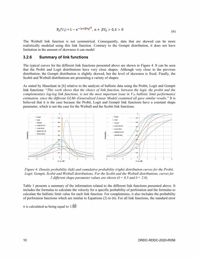
The typical curves for the different link functions presented above are shown in Figure 4. It can be seen
that the Probit and Logit distributions have very close shapes. Although very close to the previous
distribution, the Gompit distribution is slightly skewed, but the level of skewness is fixed. Finally, the
Scobit and Weibull distributions are presenting a variety of shapes.
As stated by Mauchant in [6] relative to the analysis of ballistic data using the Probit, Logit and Gompit
link functions: “This work shows that the choice of link function, between the logit, the probit and the
complementary log-log link functions, is not the most important issue in V50 ballistic limit performance
estimation, since the different GLMs (Generalized Linear Model) examined all gave similar results.” It is
believed that it is the case because the Probit, Logit and Gompit link functions have a constant shape
parameter, which is not the case for the Weibull and the Scobit link functions.
Figure 4: Density probability (left) and cumulative probability (right) distribution curves for the Probit,
Logit, Gompit, Scobit and Weibull distributions. For the Scobit and the Weibull distributions, curves for
2 different shape parameter values are shown (δ = 0.5 and δ = 2.0).
Table 1 presents a summary of the information related to the different link functions presented above. It
includes the formulas to calculate the velocity for a specific probability of perforation and the formulas to
calculate the ballistic limit value for each link function. For completeness, it also includes the probability
of perforation functions which are similar to Equations (2) to (6). For all link functions, the standard error
σ is calculated as being equal to 1/
DRDC-RDDC-2020-R056 11
Table 1: Summary of link function characteristics and ballistic limit formula.
Link
function
name
Probability of
perforation at
velocity VS
Probability
scaling
(
Velocity (VS) at
probability of
perforation P
Ballistic limit value
estimation
Probit
Φ-1(P) (Φ-1(P)- )/ - /
Logit
- /
Gompit (-0.3665 - )/
Scobit
Weibull
3.3 Fitting Process Calculations
3.3.1 General
The program takes the VS versus Response data and fits the above
defined link functions to the data The fitting process consists of finding the estimates of the parameters
(α, β, δ) that maximise the likelihood that the fitted curve corresponds to the experimental data
(Maximum Likelihood Estimation, ML). The search for the optimal values of α, β and δ is done using
the Downhill Simplex algorithm. The Simplex method published by Nelder and Mead [7] is a
single-objective optimization approach for searching the space of n-dimensional real vectors. It only uses
the values of the objective functions without any derivative information and therefore, it falls into the
general class of direct search methods. The absence of derivative information in this method makes it
suitable for problems with non-smooth functions and discontinuous functions which occurs frequently in
statistics and experimental mathematics.
12 DRDC-RDDC-2020-R056
The Simplex method is simplex-based. A simplex S in Rn is defined as the convex hull of n+1 vertices x0,
x1, … xn ϵ Rn. For example, a simplex in R1 is a line, in R2 is a triangle, and in R3 is a tetrahedron. For the
case of the cumulative normal equation (Probit), the dimension n of the simplex is 2 (α and β). The
method begins with a working simplex S and the corresponding set of function values at the vertices ƒ(xj)
for j = 0, 1, …, n. The function ƒ is the maximum likelihood equation. The method then performs a
sequence of transformations of the working simplex aimed at decreasing the function values at its
vertices. At each step, the transformation is determined by computing one or more test points, together
with their function values, and by comparison of these function values with those at the vertices.
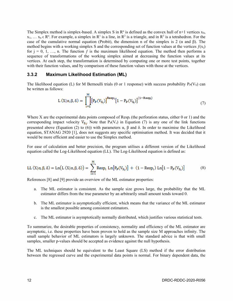
3.3.2 Maximum Likelihood Estimation (ML)
The likelihood equation (L) for M Bernoulli trials (0 or 1 response) with success probability PP(VS) can
be written as follows:
(7)
Where X are the experimental data points composed of Respi (the perforation status, either 0 or 1) and the
corresponding impact velocity . Note that PP(Vs) in Equation (7) is any one of the link functions
presented above (Equation (2) to (6)) with parameters α, β and δ. In order to maximise the Likelihood
equation, STANAG 2920 [1], does not suggests any specific optimisation method. It was decided that it
would be more efficient and easier to use the Simplex method.
For ease of calculation and better precision, the program utilises a different version of the Likelihood
equation called the Log-Likelihood equation (LL). The Log-Likelihood equation is defined as:
(8)
References [8] and [9] provide an overview of the ML estimator properties:
a. The ML estimator is consistent. As the sample size grows large, the probability that the ML
estimator differs from the true parameter by an arbitrarily small amount tends toward 0.
b. The ML estimator is asymptotically efficient, which means that the variance of the ML estimator
is the smallest possible among consistent estimators.
c. The ML estimator is asymptotically normally distributed, which justifies various statistical tests.
To summarize, the desirable properties of consistency, normality and efficiency of the ML estimator are
asymptotic, i.e. these properties have been proven to hold as the sample size M approaches infinity. The
small sample behavior of ML estimators is largely unknown. The standard advice is that with small
samples, smaller p-values should be accepted as evidence against the null hypothesis.
The ML techniques should be equivalent to the Least Square (LS) method if the error distribution
between the regressed curve and the experimental data points is normal. For binary dependent data, the

DRDC-RDDC-2020-R056 13
error distribution is not normal and therefore both techniques are not equivalent. Furthermore, in ballistic
applications, the data set is typically small or moderate in size (less than 500 data points) which induces a
bias in the estimations, resulting in models that are not equivalent
Some simulation studies have shown that for small data size where there are only a few failures, the ML
method is better than the LS method [10]. Also, some authors have shown that for binary dependent data,
the error distribution might not follow the normal distribution [11]. Therefore, the ML method is used by
this program. It should be considered that the model that results in the lowest standard error on the V50,
SD and fit values should be more accurate.
3.4 Confidence Interval and Standard Error Calculation
3.4.1 General
There are three different methods used to calculated the confidence limits in BLC. The first is explained
in details in STANAG 2920 ([1], [2]) and won’t be detailed further herein. The results of that process for
the ballistic limit and the standard deviation values is shown in the “Results 1” sheet for each link
functions on the 5 lines labeled “STANAG 2920 method”.
The second and third are explained in the subsection on Confidence interval curves below and the result
of that process for each link functions are shown in the “Results 1” sheet on the 3 lines labeled either
“Normal CI curves” (the second method) or “Binomial CI curves” (the third method). The first line
presents the Confidence Interval length for 50% probability of perforation whereas the second line and
third line presents the maximal and minimal ballistic limit values for the selected Confidence Level and
assumed error distribution. Other results of the second or third process are presented in the “Results 2”
sheet under the headings “CL Upper” and “CL Lower” for each link functions and presented graphically
on the graphics sheets named Probit, Logit, Scobit, Gompt and Weibull.
For the second method that assumes the Normal distribution of the error , it is first necessary to evaluate
the standard error of the different fitted parameters. The process to estimate the standard error is therefore
explained first.
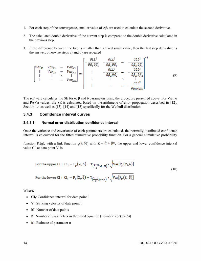
3.4.2 Standard Error Estimation
Standard errors (SE) are calculated based on the estimated variance (Var) and covariance of the fitted
parameters ( ). The variance of an equation with N parameters (βi, i = 1 to N) is
given by Equation (9). Notice that the variance/covariance matrix is symetric and that all the values of the
diagonal are positive while the others can be either positive or negative. Once the best fit parameters for
each link functions are defined using the ML technique, a numerical double derivative of the LL function
is calculated for each parameters. The double derivatives are calculated using a 5 points central stencil
with a truncation error O(Δβi4) for the unidirectional derivatives and a 4 points central stencil with a
truncation error O(Δβi2, Δβj
2), i ≠ j for the cross derivatives.
To minimize errors in the double derivative calculation, the double derivatives are calculated by a
convergence algorithm that optimises the balance between the round-off error of the computer arithmetic
and the truncation error of the double derivative. Briefly, the convergence algorithm works as follows:
14 DRDC-RDDC-2020-R056
1. For each step of the convergence, smaller value of Δβi are used to calculate the second derivative.
2. The calculated double derivative of the current step is compared to the double derivative calculated in
the previous step.
3. If the difference between the two is smaller than a fixed small value, then the last step derivative is
the answer, otherwise steps a) and b) are repeated
(9)
The software calculates the SE for α, β and δ parameters using the procedure presented above. For V50 , σ
and PP(Vi) values, the SE is calculated based on the arithmetic of error propagation described in [12],
Section 1.4 as well as [13], [14] and [15] specifically for the Weibull distribution.
3.4.3 Confidence interval curves
3.4.3.1 Normal error distribution confidence interval
Once the variance and covariance of each parameters are calculated, the normally distributed confidence
interval is calculated for the fitted cumulative probability function. For a general cumulative probability
function Pp(g), with a link function g( ) with Z = , the upper and lower confidence interval
value CIi at data point Vi is:
(10)
Where:
CIi: Confidence interval for data point i
Vi: Striking velocity of data point i
M: Number of data points
N: Number of parameters in the fitted equation (Equations (2) to (6))
: Estimate of parameter α
DRDC-RDDC-2020-R056 15
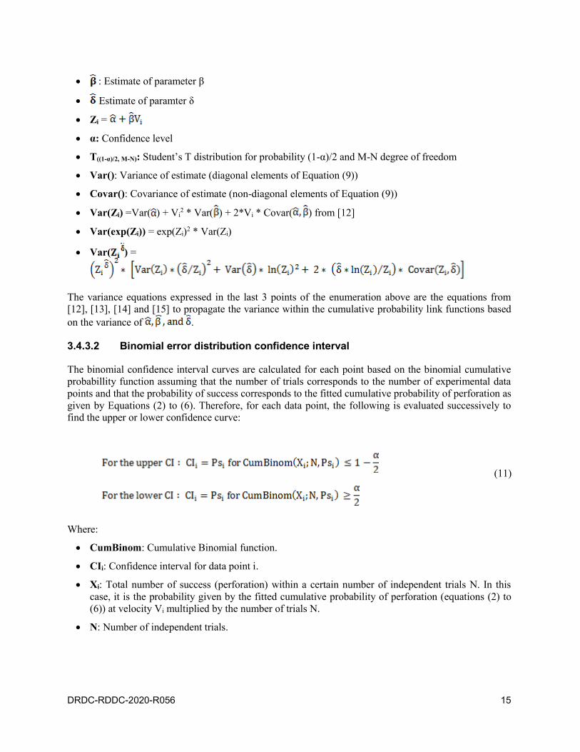
: Estimate of parameter β
Estimate of paramter δ
Zi =
α: Confidence level
T((1-α)/2, M-N): Student’s T distribution for probability (1-α)/2 and M-N degree of freedom
Var(): Variance of estimate (diagonal elements of Equation (9))
Covar(): Covariance of estimate (non-diagonal elements of Equation (9))
Var(Zi) =Var( ) + Vi2 * Var( ) + 2*Vi * Covar( ) from [12]
Var(exp(Zi)) = exp(Zi)2 * Var(Zi)
Var( ) =
The variance equations expressed in the last 3 points of the enumeration above are the equations from
[12], [13], [14] and [15] to propagate the variance within the cumulative probability link functions based
on the variance of .
3.4.3.2 Binomial error distribution confidence interval
The binomial confidence interval curves are calculated for each point based on the binomial cumulative
probabillity function assuming that the number of trials corresponds to the number of experimental data
points and that the probability of success corresponds to the fitted cumulative probability of perforation as
given by Equations (2) to (6). Therefore, for each data point, the following is evaluated successively to
find the upper or lower confidence curve:
(11)
Where:
CumBinom: Cumulative Binomial function.
CIi: Confidence interval for data point i.
Xi: Total number of success (perforation) within a certain number of independent trials N. In this
case, it is the probability given by the fitted cumulative probability of perforation (equations (2) to
(6)) at velocity Vi multiplied by the number of trials N.
N: Number of independent trials.

16 DRDC-RDDC-2020-R056
: Probability of success for each independent trails.
For the upper CI, the value of is varied from 0.999 to 0 and Equation (11) is evaluated until the
condition for the upper CI is true. For the lower CI, the value of is varied from 0 to 0.999 and
Equation (11) is evaluated until the condition for the lower CI is true.
DRDC-RDDC-2020-R056 17
4 Diagnostic tools
4.1 General
With the fitted parameters, the ballistic limit and standard deviation values and their standard error, BLC
also executes a series of tests to assess:
Information on the data sample
Tests to assess the validity of the data for use with the different tests below
The goodness of fit of the link functions to the data points
The significance of the fitted parameters
The following sections will describe the different diagnostic tools used in BLC.
4.2 Information on the data sample
Information on the data sample can be found under the heading “SAMPLE STATISTICS” of the
“Results 1” sheet and on the Box Plot sheet.
4.2.1 Sample Statistics section of the “Results 1” sheet
The data included in that section are:
Sample median: The velocity value that splits the ordered data sample in two halfs. Within the
sample, 50% of the data points are higher and 50% of the data points are lower than that velocity.
Sample mean: The average of all velocities .
Sample standard deviation: The standard deviation of the sample .
Spread: Defined as the difference between the highest impact velocity and the lowest impact
velocity of the data sample.
LC: Velocity of the lowest complete perforation within the sample
HP: Velocity of the highest partial perforation within the sample
ZMR: Zone of mixed results defined as the difference between HP and LC of the data sample. If the
value is negative, then there is no ZMR (ZMR = 0)
Skewness: Measure of the symmetry of the sample. It is defined as (this
is the Fisher-Pearson adjusted coefficient of skewness, adjusted for sample size [16]) That value can
18 DRDC-RDDC-2020-R056
be positive or negative. For a positive skewness or right-skewed sample, the longest tail of the
sample density function is at the right of the distribution and the mean of the sample is at the right of
the median (higher than the median) of the sample. Inversely, for a negative skewness or
left-skewed sample, the longest tail of the sample density function is at the left of the distribution
and the mean of the sample is at the left of the median (lower than the median) of the sample. A
sample skewness of 0 or near 0 indicates symmetry. Based on [17], the skewness value can be
interpreted as:
If skewness is between −½ and +½, then the distribution is approximately symmetric
If skewness is less than -1 or higher than +1, then the distribution is highly skewed
If the skewness is between −½ and -1 or between +½ and +1 then the distribution is
moderately skewed.
Kurtosis: Measure of the heaviness of the sample distribution tails. It is defined as
(this is actually the excess kurtosis as discussed in [16]) That value can be
positive or negative. A value of 0 indicates that the tails of the sample distribution are identical to
the tail of a standard normal distribution. Positive kurtosis indicates that the tails of the sample
distribution are heavier than the tail of a normal density distribution. Inversely, negative kurtosis
kurtosis indicates that the tails of the sample distribution are lighter than the tail of a standard
normal distribution [16].
Number of data points: Indicates the number of data points used in the calculation.
4.2.2 Box Plot sheet
A summary of the data are displayed graphically on the “Box Plot” sheet. That chart presents the
following information:
Maximum (“Max” label) and minimum (“Min” label) impact velocities of the sample
The median, first quartile (“Q1” label) and third quartile (“Q3” label) values of the sample
The interquartile range (“IQR” label). It is defined as the difference between Q3 and Q1
The sample mean value (“Mean” label), marked with a blue “X” on the chart
Vertical bars outside the Q3-Q1 box that describe the 1.5 IQR limit above and below Q3 and Q1
respectively. Data points outside those bars are sometimes designated as outliers by some authors
Data points that are outside the Q1-Q3 range
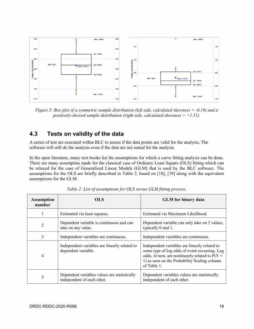
The Box plot chart can be used to assess the sample characteristics. If the distance Median-Q3 and
Median-Max is about the same as the distance Median-Q1 and Median-Min, and that the Mean value is
about the same as the Median value, then the sample distribution is almost symmetric (see Figure 5 left
side). If it is not the case, the data is skewed either negatively or positively (see Figure 5 right side).
DRDC-RDDC-2020-R056 19
Figure 5: Box plot of a symmetric sample distribution (left side, calculated skewness = -0.19) and a
positively-skewed sample distribution (right side, calculated skewness = +1.51).
4.3 Tests on validity of the data
A series of test are executed within BLC to assess if the data points are valid for the analysis. The
software will still do the analysis even if the data are not suited for the analysis.
In the open literature, many text books list the assumptions for which a curve fitting analysis can be done.
There are many assumptins made for the classical case of Ordinary Least Square (OLS) fitting which can
be relaxed for the case of Generalized Linear Models (GLM) that is used by the BLC software. The
assumptions for the OLS are briefly described in Table 2, based on [18], [19] along with the equivalent
assumptions for the GLM.
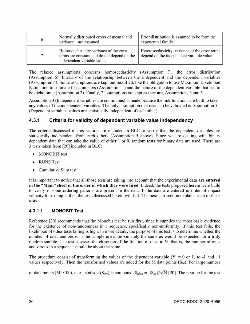
Table 2: List of assumptions for OLS versus GLM fitting process.
Assumption
number
OLS GLM for binary data
1 Estimated via least squares. Estimated via Maximum Likelihood.
2 Dependent variable is continuous and can
take on any value.
Dependent variable can only take on 2 values,
typically 0 and 1.
3 Independent variables are continuous. Independent variables are continuous.
4
Independent variables are linearly related to
dependent variable.
Independent variables are linearly related to
some type of log odds of event occurring. Log
odds, in turn, are nonlinearly related to P(Y =
1) as seen on the Probability Scaling column
of Table 1.
5 Dependent variables values are statistically
independent of each other.
Dependent variables values are statistically
independent of each other.
20 DRDC-RDDC-2020-R056
6 Normally distributed errors of mean 0 and
variance 1 are assumed.
Error distribution is assumed to be from the
exponential family.
7
Homoscedasticity: variance of the error
terms are constant and do not depend on the
independent variable value.
Heteroscedasticity: variance of the error terms
depend on the independent variable value.
The relaxed assumptions concerns homoscedasticity (Assumption 7), the error distribution
(Assumption 6), linearity of the relationship between the independent and the dependent variables
(Assumption 4). Some assumptions are kept but modified, like the obligation to use Maximum Likelihood
Estimation to estimate fit parameters (Assumption 1) and the nature of the dependent variable that has to
be dichotomic (Assumption 2). Finally, 2 assumptions are kept as they are, Assumptions 3 and 5.
Assumption 3 (Independent variables are continuous) is made because the link functions are built to take
any values of the independent variables. The only assumption that needs to be validated is Assumption 5
(Dependent variables values are statistically independent of each other)
4.3.1 Criteria for validity of dependent variable value independency
The criteria discussed in this section are included in BLC to verify that the dependent variables are
statistically independent from each others (Assumption 5 above). Since we are dealing with binary
dependent data that can take the value of either 1 or 0, random tests for binary data are used. There are
3 tests taken from [20] included in BLC:
MONOBIT test
RUNS Test
Cumulative Sum test
It is important to notice that all those tests are taking into account that the experimental data are entered
in the “Main” sheet in the order in which they were fired. Indeed, the tests proposed herein were build
to verify if some ordering patterns are present in the data. If the data are entered in order of impact
velocity for example, then the tests discussed herein will fail. The next sub-section explains each of these
tests.
4.3.1.1 MONOBIT Test
Reference [20] recommends that the Monobit test be run first, since it supplies the most basic evidence
for the existence of non-randomness in a sequence, specifically non-uniformity. If this test fails, the
likelihood of other tests failing is high. In more details, the purpose of this test is to determine whether the
number of ones and zeros in the sample are approximately the same as would be expected for a truly
random sample. The test assesses the closeness of the fraction of ones to ½, that is, the number of ones
and zeroes in a sequence should be about the same.
The procedure consist of transforming the values of the dependent variable (Yj = 0 or 1) to -1 and +1
values respectively. Then the transformed values are added for the M data points (SM). For large number
of data points (M ≥100), a test statistic (Sobs) is computed: [20]. The p-value for the test
DRDC-RDDC-2020-R056 21
statistic is then calculated: , where erfc is the complementary error
function. For small number of data points [21], the statistic is calculated and its p-value is
calculated from the cumulative binomial distribution of the statistic for M data points and the probability
of occurrence of ½.
If the computed p-value is < α, then conclude that the sequence is non-random. Otherwise, conclude that
the sequence is random.
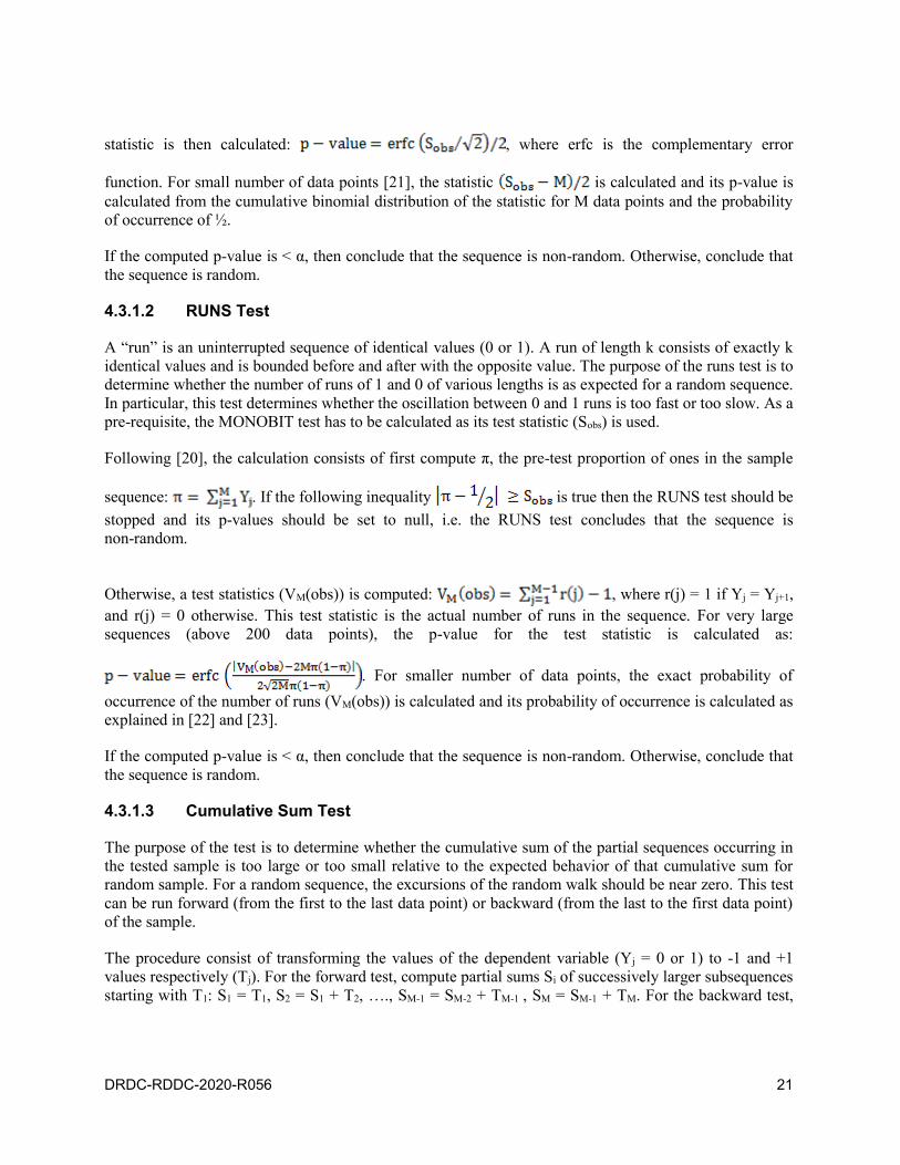
4.3.1.2 RUNS Test
A “run” is an uninterrupted sequence of identical values (0 or 1). A run of length k consists of exactly k
identical values and is bounded before and after with the opposite value. The purpose of the runs test is to
determine whether the number of runs of 1 and 0 of various lengths is as expected for a random sequence.
In particular, this test determines whether the oscillation between 0 and 1 runs is too fast or too slow. As a
pre-requisite, the MONOBIT test has to be calculated as its test statistic (Sobs) is used.
Following [20], the calculation consists of first compute π, the pre-test proportion of ones in the sample
sequence: . If the following inequality is true then the RUNS test should be
stopped and its p-values should be set to null, i.e. the RUNS test concludes that the sequence is
non-random.
Otherwise, a test statistics (VM(obs)) is computed: , where r(j) = 1 if Yj = Yj+1,
and r(j) = 0 otherwise. This test statistic is the actual number of runs in the sequence. For very large
sequences (above 200 data points), the p-value for the test statistic is calculated as:
. For smaller number of data points, the exact probability of
occurrence of the number of runs (VM(obs)) is calculated and its probability of occurrence is calculated as
explained in [22] and [23].
If the computed p-value is < α, then conclude that the sequence is non-random. Otherwise, conclude that
the sequence is random.
4.3.1.3 Cumulative Sum Test
The purpose of the test is to determine whether the cumulative sum of the partial sequences occurring in
the tested sample is too large or too small relative to the expected behavior of that cumulative sum for
random sample. For a random sequence, the excursions of the random walk should be near zero. This test
can be run forward (from the first to the last data point) or backward (from the last to the first data point)
of the sample.
The procedure consist of transforming the values of the dependent variable (Yj = 0 or 1) to -1 and +1
values respectively (Tj). For the forward test, compute partial sums Si of successively larger subsequences
starting with T1: S1 = T1, S2 = S1 + T2, …., SM-1 = SM-2 + TM-1 , SM = SM-1 + TM. For the backward test,
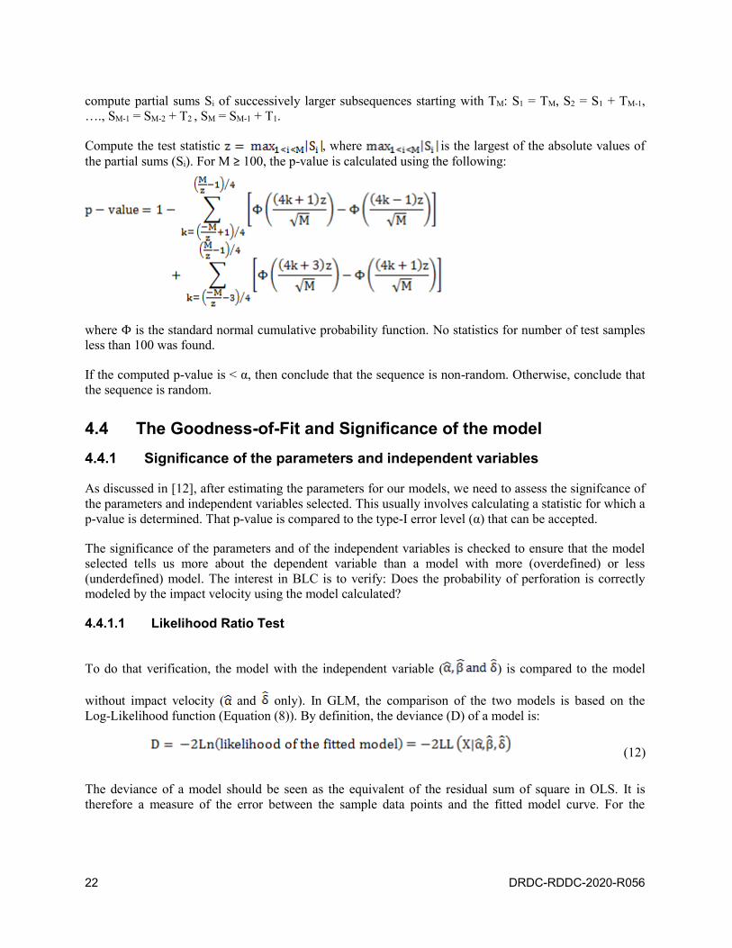
22 DRDC-RDDC-2020-R056
compute partial sums Si of successively larger subsequences starting with TM: S1 = TM, S2 = S1 + TM-1,
…., SM-1 = SM-2 + T2 , SM = SM-1 + T1.
Compute the test statistic , where is the largest of the absolute values of
the partial sums (Si). For M ≥ 100, the p-value is calculated using the following:
where Φ is the standard normal cumulative probability function. No statistics for number of test samples
less than 100 was found.
If the computed p-value is < α, then conclude that the sequence is non-random. Otherwise, conclude that
the sequence is random.
4.4 The Goodness-of-Fit and Significance of the model
4.4.1 Significance of the parameters and independent variables
As discussed in [12], after estimating the parameters for our models, we need to assess the signifcance of
the parameters and independent variables selected. This usually involves calculating a statistic for which a
p-value is determined. That p-value is compared to the type-I error level (α) that can be accepted.
The significance of the parameters and of the independent variables is checked to ensure that the model
selected tells us more about the dependent variable than a model with more (overdefined) or less
(underdefined) model. The interest in BLC is to verify: Does the probability of perforation is correctly
modeled by the impact velocity using the model calculated?
4.4.1.1 Likelihood Ratio Test
To do that verification, the model with the independent variable ( ) is compared to the model
without impact velocity ( and only). In GLM, the comparison of the two models is based on the
Log-Likelihood function (Equation (8)). By definition, the deviance (D) of a model is:
(12)
The deviance of a model should be seen as the equivalent of the residual sum of square in OLS. It is
therefore a measure of the error between the sample data points and the fitted model curve. For the
DRDC-RDDC-2020-R056 23
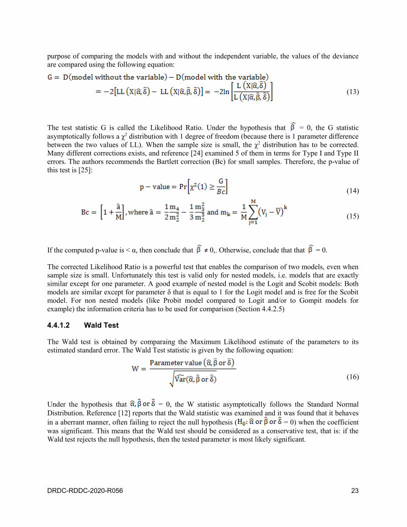
purpose of comparing the models with and without the independent variable, the values of the deviance
are compared using the following equation:
(13)
The test statistic G is called the Likelihood Ratio. Under the hypothesis that = 0, the G statistic
asymptotically follows a χ2 distribution with 1 degree of freedom (because there is 1 parameter difference
between the two values of LL). When the sample size is small, the χ2 distribution has to be corrected.
Many different corrections exists, and reference [24] examined 5 of them in terms for Type I and Type II
errors. The authors recommends the Bartlett correction (Bc) for small samples. Therefore, the p-value of
this test is [25]:
(14)
(15)
If the computed p-value is < α, then conclude that ≠ 0,. Otherwise, conclude that that = 0.
The corrected Likelihood Ratio is a powerful test that enables the comparison of two models, even when
sample size is small. Unfortunately this test is valid only for nested models, i.e. models that are exactly
similar except for one parameter. A good example of nested model is the Logit and Scobit models: Both
models are similar except for parameter δ that is equal to 1 for the Logit model and is free for the Scobit
model. For non nested models (like Probit model compared to Logit and/or to Gompit models for
example) the information criteria has to be used for comparison (Section 4.4.2.5)
4.4.1.2 Wald Test
The Wald test is obtained by comparaing the Maximum Likelihood estimate of the parameters to its
estimated standard error. The Wald Test statistic is given by the following equation:
(16)
Under the hypothesis that = 0, the W statistic asymptotically follows the Standard Normal
Distribution. Reference [12] reports that the Wald statistic was examined and it was found that it behaves
in a aberrant manner, often failing to reject the null hypothesis ( = 0) when the coefficient
was significant. This means that the Wald test should be considered as a conservative test, that is: if the
Wald test rejects the null hypothesis, then the tested parameter is most likely significant.
24 DRDC-RDDC-2020-R056
4.4.2 Goodness-of-Fit Tests
Goodness-of-Fit tests are use to assess if the values predicted by the model are representative of the
experimental values in the absolute sense.
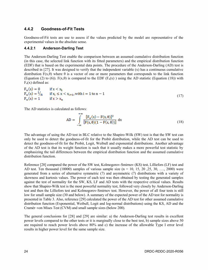
4.4.2.1 Anderson-Darling Test
The Anderson-Darling Test enable the comparison between an assumed cumulative distribution function
(in this case, the selected link function with its fitted parameters) and the empirical distribution function
(EDF) that is based on the experimental data points. The procedure of the Anderson-Darling (AD) test is
described in [27]. It was designed to verify that the independent variable (x) has a continuous cumulative
distribution F(x,θ) where θ is a vector of one or more parameters that corresponds to the link function
(Equation (2) to (6)). F(x,θ) is compared to the EDF (Fn(x) ) using the AD statistic (Equation (18)) with
Fn(x) defined as:
(17)
The AD statistics is calculated as follows:
(18)
The advantage of using the AD test in BLC relative to the Shapiro-Wilk (SW) test is that the SW test can
only be used to detect the goodness-of-fit for the Probit distribution, while the AD test can be used to
detect the goodness-of-fit for the Probit, Logit, Weibull and exponential distributions. Another advantage
of the AD test is that its weight function is such that it usually makes a more powerful test statistic by
emphasizing the tail differences between the empirical distribution function and the assumed cumulative
distribution function.
Reference [28] compared the power of the SW test, Kolmogorov-Smirnov (KS) test, Lilliefors (LF) test and
AD test. Ten thousand (10000) samples of various sample size (n = 10, 15, 20 ,25, 30, …., 2000) were
generated from a series of alternative symmetric (7) and asymmetric (7) distributions with a variety of
skewness and kurtosis values. The power of each test was then obtained by testing the generated samples
against the test of normality for the SW, KS, LF and AD tests with the respective critical values. Results
show that Shapiro-Wilk test is the most powerful normality test, followed very closely by Anderson-Darling
test and then the Lilliefors test and Kolmogorov-Smirnov test. However, the power of all four tests is still
low for small sample size (30 and below). A summary of the expected power of the AD test for normality is
presented in Table 3. Also, reference [29] calculated the power of the AD test for other assumed cumulative
distribution function (Exponential, Weibull, Logit and log-normal distributions) using the KS, AD and the
Cramér–von Mises Test (CVM) and small sample sizes (below 200).
The general conclusions for [28] and [29] are similar: a) the Anderson-Darling test results in excellent
power levels compared to the other tests or it is marginally close to the best test, b) sample sizes above 50
are required to reach power levels above 80% and c) the increase of the allowable Type I error level
results in higher power level for the same sample size.
DRDC-RDDC-2020-R056 25
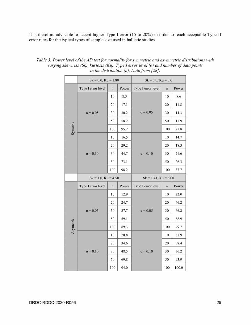
It is therefore advisable to accept higher Type I error (15 to 20%) in order to reach acceptable Type II
error rates for the typical types of sample size used in ballistic studies.
Table 3: Power level of the AD test for normality for symmetric and asymmetric distributions with
varying skewness (Sk), kurtosis (Ku), Type I error level (α) and number of data points
in the distribution (n). Data from [28].
Sk = 0.0, Ku = 1.80 Sk = 0.0, Ku = 5.0
Sy
met
ric
Type I error level n Power Type I error level n Power
α = 0.05
10 8.5
α = 0.05
10 8.6
20 17.1 20 11.8
30 30.2 30 14.3
50 58.2 50 17.9
100 95.2 100 27.8
α = 0.10
10 16.5
α = 0.10
10 14.7
20 29.2 20 18.3
30 44.7 30 21.6
50 73.1 50 26.3
100 98.2 100 37.7
Sk = 1.0, Ku = 4.50 Sk = 1.41, Ku = 6.00
Asy
met
ric
Type I error level n Power Type I error level n Power
α = 0.05
10 12.9
α = 0.05
10 22.0
20 24.7 20 46.2
30 37.7 30 66.2
50 59.1 50 88.9
100 89.3 100 99.7
α = 0.10
10 20.8
α = 0.10
10 31.9
20 34.6 20 58.4
30 48.5 30 76.2
50 69.8 50 93.9
100 94.0 100 100.0
26 DRDC-RDDC-2020-R056
4.4.2.2 Sensitivity, Specificity and area under the ROC curve (AUC)
The use of Sensitivity,Specificity and AUC tries to answer the following question: How good a job the
model does of predicting outcomes? Or said anotherway: What percent of the observations the model
correctly predicts? Can my model discriminates between positive and negative outcomes?
These questions can be answered by measuring how good the model is to measure true positive and true
negative answers while minimizing the number of false positive and false negative. All of these are
calculated by comparing the model outcome to the sample measured outcome
But first, here are some definitions:
1. Sensitivity (or true positive rate) is the proportion of positives (complete perforation) correctly
identified by the model. This value has to be has high a possible.
2. Specificity (or true negative rate) is the proportion of negative (partial perforation) correctly
identified by the model. This value has to be has high a possible. On contrary the value of
1-Specificity is the false negative rate, and it has to be as small as possible
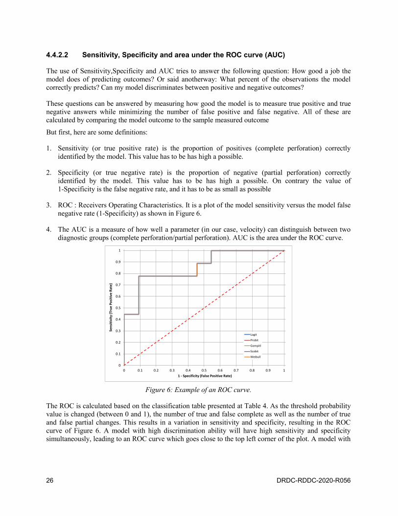
3. ROC : Receivers Operating Characteristics. It is a plot of the model sensitivity versus the model false
negative rate (1-Specificity) as shown in Figure 6.
4. The AUC is a measure of how well a parameter (in our case, velocity) can distinguish between two
diagnostic groups (complete perforation/partial perforation). AUC is the area under the ROC curve.
0
0.1
0.2
0.3
0.4
0.5
0.6
0.7
0.8
0.9
1
0 0.1 0.2 0.3 0.4 0.5 0.6 0.7 0.8 0.9 1
Sen
siti
vity
(Tr
ue
Po
siti
ve R
ate
)
1 - Specificity (False Positive Rate)
Logit
Probit
Gompitl
Scobit
Weibull
Figure 6: Example of an ROC curve.
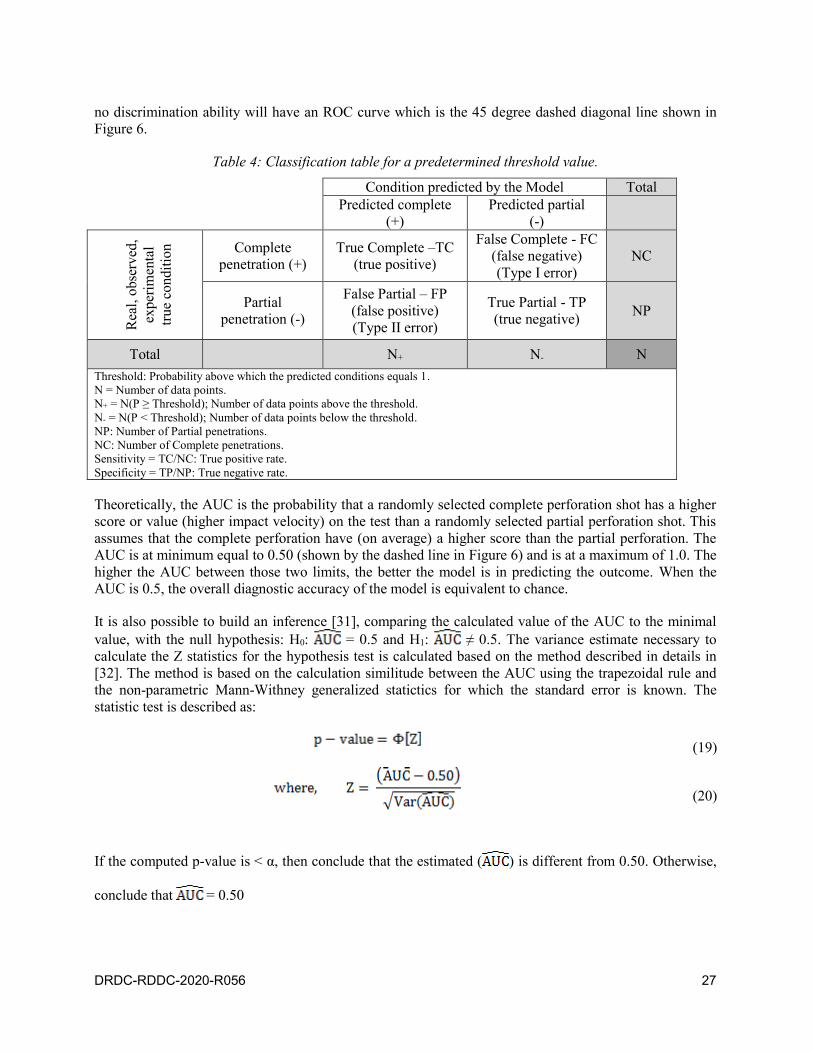
The ROC is calculated based on the classification table presented at Table 4. As the threshold probability
value is changed (between 0 and 1), the number of true and false complete as well as the number of true
and false partial changes. This results in a variation in sensitivity and specificity, resulting in the ROC
curve of Figure 6. A model with high discrimination ability will have high sensitivity and specificity
simultaneously, leading to an ROC curve which goes close to the top left corner of the plot. A model with
DRDC-RDDC-2020-R056 27
no discrimination ability will have an ROC curve which is the 45 degree dashed diagonal line shown in
Figure 6.
Table 4: Classification table for a predetermined threshold value.
Condition predicted by the Model Total
Predicted complete
(+)
Predicted partial
(-)
Rea
l, o
bse
rved
,
exp
erim
enta
l
tru
e co
ndit
ion
Complete
penetration (+)
True Complete –TC
(true positive)
False Complete - FC
(false negative)
(Type I error)
NC
Partial
penetration (-)
False Partial – FP
(false positive)
(Type II error)
True Partial - TP
(true negative) NP
Total N+ N- N
Threshold: Probability above which the predicted conditions equals 1.
N = Number of data points.
N+ = N(P ≥ Threshold); Number of data points above the threshold.
N- = N(P < Threshold); Number of data points below the threshold.
NP: Number of Partial penetrations.
NC: Number of Complete penetrations.
Sensitivity = TC/NC: True positive rate.
Specificity = TP/NP: True negative rate.
Theoretically, the AUC is the probability that a randomly selected complete perforation shot has a higher
score or value (higher impact velocity) on the test than a randomly selected partial perforation shot. This
assumes that the complete perforation have (on average) a higher score than the partial perforation. The
AUC is at minimum equal to 0.50 (shown by the dashed line in Figure 6) and is at a maximum of 1.0. The
higher the AUC between those two limits, the better the model is in predicting the outcome. When the
AUC is 0.5, the overall diagnostic accuracy of the model is equivalent to chance.
It is also possible to build an inference [31], comparing the calculated value of the AUC to the minimal
value, with the null hypothesis: H0: = 0.5 and H1: ≠ 0.5. The variance estimate necessary to
calculate the Z statistics for the hypothesis test is calculated based on the method described in details in
[32]. The method is based on the calculation similitude between the AUC using the trapezoidal rule and
the non-parametric Mann-Withney generalized statictics for which the standard error is known. The
statistic test is described as:
(19)
(20)
If the computed p-value is < α, then conclude that the estimated ( ) is different from 0.50. Otherwise,
conclude that = 0.50

28 DRDC-RDDC-2020-R056
4.4.2.3 The Stukel Test
The Stukel Test [12], [30] works only for the Logit link function. It consist of adding two parameters to
the Logit equation to make it more general (Generalized Logistic Model). Again, those additional
parameters are giving weight to the tails of the Logit distribution. The 4 parameter equation is then fitted
using the ML estimation technique and its resulting likelihood is compared to the likelihood of the
standard Logit (Equation (4)) using the likelihood ratio test described is Section 4.4.1.1. If the ratio is not
significant, then the two additional paramters are not significant, which means that the sample data at the
tails of the distribution are well described by the Logit model.
The test can be briefly described as
1. Fit the data sample using the Logit link function (Equation (3))
2. Using the fitted parameters, create two new variables (za and zb):
If
3. Fit the data sample using the Generalized Logistic Model:
4. Calculated the Log Likelihood Ratio (G) statistic
5. Find the p-value of the G statistic using Equations (14) and (15).
Reference [30] compared the power of the Stukel test relative to 8 other tests for the Logit link function
using Monte Carlo simulations of 15 different symmetric and asymmetric distributions with 100 and
500 data points. The authors recommend the use of the Stukel Test to detect departure from Logistic
distribution. Similarly to the Anderson-Darling Test above, the authors also add that “In all cases one
must keep in mind the lack of power with small sample sizes to detect subtle deviations from the logistic
model”. With this in mind the same conclusion as for the Anderson=Darling Test holds here: It is
therefore advisable to accept higher Type I error (15 to 20%) in order to reach acceptable Type II error
rates for the typical types of sample size used in ballistic studies.
4.4.2.4 Pseudo-R2
The use of R2,the coefficient of determination, is well established in classical regression analysis (OLS).
By definition it is the proportion of the dependent variable variance 'explained' by the regression model to
the total variance of the dependent variable observed. It is therefore useful as a measure of success of
predicting the dependent variable from the independent variables. Unfortunately, that definition is invalid
for GLM because of the invalidity of the total Sum of Square equation: Sum of Square Regression + Sum
of Square Error = Sum of Square Total
DRDC-RDDC-2020-R056 29
The extension of R2 to generalized linear models (GLMs) and other more general models is not
straightforward. Different perspectives led to several generalizations to the coefficient of determination.
In BLC, 2 pseudo-R2 are presented: Nagelkerke and Tjur.
The Nagelkerke pseudo-R2 should be seen as a measure of the improvement from null model to the fitted
model. It is based on the following equation:
Actually, R2N is the ratio of the Cox and Snell pseudo-R2 (R2
CS) to the maximum possible value for R2CS
which is R2max. This value lies between 0 and 1. The R2
CS value contains the L0/L1 ratio which is the ratio
between the “null” model (containing the intercept parameter α only) to the full model (containing α, β
and δ parameters). M is the number of data points. Hence, the Nagelkerke pseudo-R2 measures the
improvement from null model to the fitted model.
The Tjur pseudo-R2 should be seen as a coefficient of discrimination: It measures the ability of the model
to discriminate between successes and failures. It is calculated as the difference in the average of the
event probabilities between the groups of observations with observed events ( ) and nonevents (( ))
To conclude this section, reference [12] provides a interesting insight in the use and the typical values of
R2 in logistic regression and GLM:
...low R2 values in logistic regression are the norm and this presents a problem when reporting
their values to an audience accustomed to seeing linear regression values. ... Thus [arguing by
reference to running examples in the text] we do not recommend routine publishing of R2 values
with results from fitted logistic models. However, they may be helpful in the model building state
as a statistic to evaluate competing models.
4.4.2.5 Information Criterion (IC): General considerations
As pointed above, the Log-Likelihood Ratio cannot be used to compare non nested models (like Probit
model compared to Logit and/or to Gompit models for example). For non nested models, the information
criterion has to be used [26]. It is based on the information theory using the Kullback-Leibler information
equation that measures the 'information' lost when approximating reality using a function. The
information criterion accounts for how well the model fits the data and also accounts for the complexity
of the model. Model complexity is its ability to fit any data set and can be approximated as the number of
parameters in the model [26]. It is well known that some models can be so complex that they can fit any
data set [26]: A model that seems to fit all data sets because it is overly complex may include so many

30 DRDC-RDDC-2020-R056
parameters that it is of little use to explain the outcome score that is of interest, which goes against the
purpose of developing models, that is to explain a particular facet of a phenomenon.
The Kullback-Leibler information ([34], [35]) or “distance” between f(x), which is a function that
represents the “full truth”or “the real model” and an approximating model gj(x) that represents a series of
M possible models (j= 1, 2, … M) is defined as the first part of Equation (21). In this case, x represents a
series of independent variable. The approximating model g(x) has p parameters (θ) that are estimated
from the finite data set x using the maximum likelihood method for example.
(21)
The quantity I(f(x), g(x)) measures the 'information' lost when g(x) is used to approximate f(x) (the truth).
If f(x)=g(x), then I(f(x), g(x))= 0, since there is no information lost when the model reflects the truth
perfectly. In reality, there is always some information that will be lost when a model is used to
approximate reality and thus l(f(x), g(x)) > 0. In reality, I(f(x), g(x)) cannot be used in that form for model
selection because it requires knowledge of the truth (f(x)) and of the parameters (θ) in g(x) = g(x|θ). But,
the relative Kullback-Leibler information can be estimated from the data based on the maximized log
likelihood function.
The Kullback-Leibler information equation can also be written as the second part of Equation (21) where
Ef is the expectation with respect to the distribution f(x) ([34], [35]). Noting that is an
unknown constant, the second part of Equation (21) can be rewritten as
, hence the above mention about the relative Kullback-
Leibler information. Takeuchi [36] found the general asymptotic relationship between the target criterion,
I(f(x), g(x))] - constant, and Ef [ln(g(x| ))] which is the expected empirical maximized Log-Likelihood. In
this case, is the MLE of model g(x) with p parameters, based on the data set x. Takeuchi result is:
(22)
The Log-Likelihood, Equation (8), is un unbiased estimator of and can therefore be used in
the evaluation of the IC. Matrices J and I are of size p x p and represents the first and second partial
derivatives of with respect to θ. The matrices are evaluated at θ = θ0, which is the value of
θ that minimizes I(f(x),g(x)) for the model g(x) over all possible values of θ (i.e. the ML estimator of θ).
The term reduces to p when the number of data points to estimate the Kullback-
Leibler becomes large.
To summarize, the Information Criteria (IC) can be written as the AIC (Akaike Information Criterion
[37]), noting that there is only a factor of 2 between the two criterion (that factor appeared for historical
reasons). AIC can asymptotically be written as:
(23)
Remember that the AIC (IC) accounts for the fitted model goodness of fit and the complexity of the
model. For comparison between models, the AIC value as to be as small as possible. As Log-Likelihood
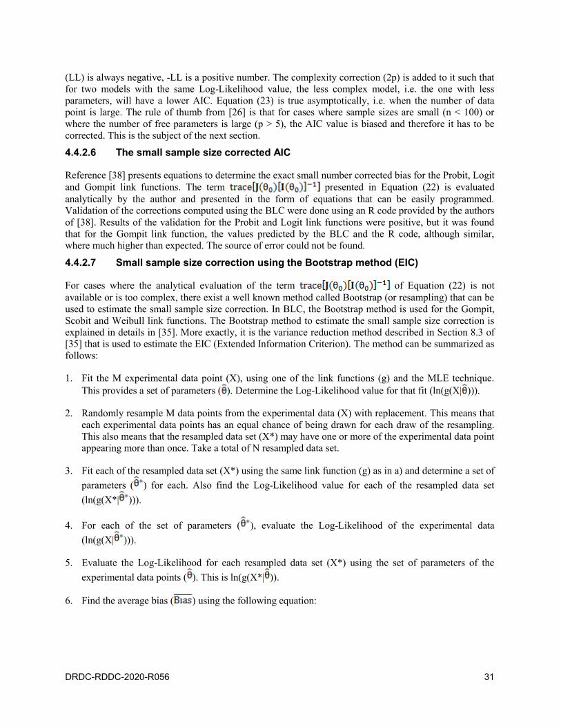
DRDC-RDDC-2020-R056 31
(LL) is always negative, -LL is a positive number. The complexity correction (2p) is added to it such that
for two models with the same Log-Likelihood value, the less complex model, i.e. the one with less
parameters, will have a lower AIC. Equation (23) is true asymptotically, i.e. when the number of data
point is large. The rule of thumb from [26] is that for cases where sample sizes are small (n < 100) or
where the number of free parameters is large (p > 5), the AIC value is biased and therefore it has to be
corrected. This is the subject of the next section.
4.4.2.6 The small sample size corrected AIC
Reference [38] presents equations to determine the exact small number corrected bias for the Probit, Logit
and Gompit link functions. The term presented in Equation (22) is evaluated
analytically by the author and presented in the form of equations that can be easily programmed.
Validation of the corrections computed using the BLC were done using an R code provided by the authors
of [38]. Results of the validation for the Probit and Logit link functions were positive, but it was found
that for the Gompit link function, the values predicted by the BLC and the R code, although similar,
where much higher than expected. The source of error could not be found.
4.4.2.7 Small sample size correction using the Bootstrap method (EIC)
For cases where the analytical evaluation of the term of Equation (22) is not
available or is too complex, there exist a well known method called Bootstrap (or resampling) that can be
used to estimate the small sample size correction. In BLC, the Bootstrap method is used for the Gompit,
Scobit and Weibull link functions. The Bootstrap method to estimate the small sample size correction is
explained in details in [35]. More exactly, it is the variance reduction method described in Section 8.3 of
[35] that is used to estimate the EIC (Extended Information Criterion). The method can be summarized as
follows:
1. Fit the M experimental data point (X), using one of the link functions (g) and the MLE technique.
This provides a set of parameters ( ). Determine the Log-Likelihood value for that fit (ln(g(X| ))).
2. Randomly resample M data points from the experimental data (X) with replacement. This means that
each experimental data points has an equal chance of being drawn for each draw of the resampling.
This also means that the resampled data set (X*) may have one or more of the experimental data point
appearing more than once. Take a total of N resampled data set.
3. Fit each of the resampled data set (X*) using the same link function (g) as in a) and determine a set of
parameters ( ) for each. Also find the Log-Likelihood value for each of the resampled data set
(ln(g(X*| ))).
4. For each of the set of parameters ( ), evaluate the Log-Likelihood of the experimental data
(ln(g(X| ))).
5. Evaluate the Log-Likelihood for each resampled data set (X*) using the set of parameters of the
experimental data points ( ). This is ln(g(X*| )).
6. Find the average bias ( ) using the following equation:
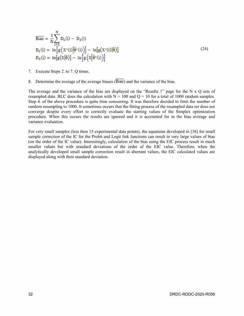
32 DRDC-RDDC-2020-R056
(24)
7. Execute Steps 2. to 7. Q times.
8. Determine the average of the average biases ( ) and the variance of the bias.
The average and the variance of the bias are displayed on the “Results 1” page for the N x Q sets of
resampled data. BLC does the calculation with N = 100 and Q = 10 for a total of 1000 random samples.
Step 4. of the above procedure is quite time consuming. It was therefore decided to limit the number of
random resampling to 1000. It sometimes occurs that the fitting process of the resampled data set does not
converge despite every effort to correctly evaluate the starting values of the Simplex optimization
procedure. When this occurs the results are ignored and it is accounted for in the bias average and
variance evaluation.
For very small samples (less then 15 experimental data points), the equations developed in [38] for small
sample correction of the IC for the Probit and Logit link functions can result in very large values of bias
(on the order of the IC value). Interestingly, calculation of the bias using the EIC process result in much
smaller values but with standard deviations of the order of the EIC value. Therefore, when the
analytically developed small sample correction result in aberrant values, the EIC calculated values are
displayed along with their standard deviation.
DRDC-RDDC-2020-R056 33
5 Results description
The principal results are provided in the “Results 1” and “Results 2” sheets. The “Results 1” sheet
contains summary data while the “Results 2” sheet displays experimental data points along with their
confidence limit values based on either a Normal or a Binomial distribution of the error.
Other summary data are provided in graphical form in the “Box Plot” sheet. In addition, raw data points
along with their fitted curves and the confidence limits curves are presented graphically in the “Probit”,
“Logit”, “Scobit”, Gompit” and “Weibull” sheets.
5.1 Summary data (“Results 1” sheet)
5.1.1 Experimental data sample statistics
This part concerns descriptive statistics of the experimental data sample
Sample median (m/s): The sample data median value.
Sample mean (m/s): The sample arithmetic mean.
Sample σ (m/s): The sample standard deviation.
Spread (m/s): The sample spread (difference between the maximum velocity value and the
minimum velocity value of the sample).
ZMR (m/s): The Zone of Mixed Results (ZMR) of the sample. It is the difference between the
highest maximum partial perforation velocity (HP) and the lowest minimum complete perforation
(LC) velocity.
LC (m/s): Lowest Complete (LC) perforation of the sample.
HP (m/s): Highest Partial (HP) perforation of the sample.
Skewness: It defines the level of skewness of the data sample, By convention, right skewed is a
positive value and results in a distribution with the longest tail to the right. Left skewed is a negative
value with the longest tail to the left of the distribution.
Kurtosis: It defines the level of kurtosis. Positive kurtosis means that the tails of the data sample
distribution are heavier than standard normal and negative kurtosis means that the tails of the data
sample distribution are lighter than standard normal.
5.1.2 Independency of dependent variable
This part of the “Results 1” sheet concerns random tests done on the experimental data sample to ensure
the mutual independence of the dependent variables. Independace of the dependent variable is one of the
important assumption of the GLM process as described in Section 4.3. The message displayed in green
means that it is a positive answer, i.e., the test sample can be assumed as random, while the message
displayed in red means that it is a negative answer, i.e., the test sample cannot be assumed as random.

34 DRDC-RDDC-2020-R056
MONOBIT Test p-value for sample randomness: Provides the result of the Monobit Test (H0:
data are randomly distributed) with the p-value related to the test statistic. The Monobit test
procedure is described in Section 4.3.1.1.
RUN Test p-value for sample randomness: Provides the result of the Run Test (H0: data are
randomly distributed) with the p-value related to the test statistic. The Run test procedure is
described in Section 4.3.1.2.
Cumulative Sum Test p-value for sample randomness: Provides the result of the Cumulative
Sum Test (H0: data are randomly distributed) with the p-value related to the test statistic. The
Cumulative Sum test procedure is described in Section 4.3.1.3.
5.1.3 Parameter values and statistics
In this part, the fitted parameter values and statistics, based on the calculations described above are
provided for each different link function.
V50 ± SE (m/s): The ballistic limit calculated from the fitted values of and (following the
equations specified in the last column of Table 1, section 3.2.6) and the calculated standard error of
the parameters as described in Section 3.4.2. are displayed.
σ ± SE (m/s): The standard deviation calculated from the fitted values of and , following the
process described in Section 3.2.6 and the calculated standard error as described in section 3.4.2.
α± SE (m/s): The value of parameter as determined for the ML fitting process along with its
standard error estimation as described in Section 3.4.2.
β± SE (m/s): The value of parameter as determined for the ML fitting process along with its
standard error estimation as described in Section 3.4.2.
δ± SE (m/s): The value of parameter as determined for the ML fitting process along with its
standard error estimation as described in Section 3.4.2.
Standard Error of Estimate at V50 (m/s): The standard error of the fitted equation:
, where p is the number of parameter in the fitted equation, is the
probability of perforation evaluated using the fitted function evaluated at velocity Vi and Pri is the
response of the material (either 0 or 1) obtained experimentally.
5.1.4 Significance of the model
The significance of the model is assessed through the evaluation of the significance of the different fitted
parameters of the model. The message displayed in green means that it is a positive answer, i.e., the
parameter is significant, while the message displayed in red means that it is a negative answer, i.e., the
parameter is not significant. The confidence level that is used to compare with the calculated p-value is
specified on the “Main” sheet (Statistical Test confidence level). The calculated p-value of the test is also
provided to give insight on how close it is to the confidence level.
Wald Test p-value on α: Result of the test of significance of the α parameter using the Wald Test as
described in Section 4.4.1.2.
Wald Test p-value on β: Result of the test of significance of the β parameter using the Wald Test as
described in Section 4.4.1.2.
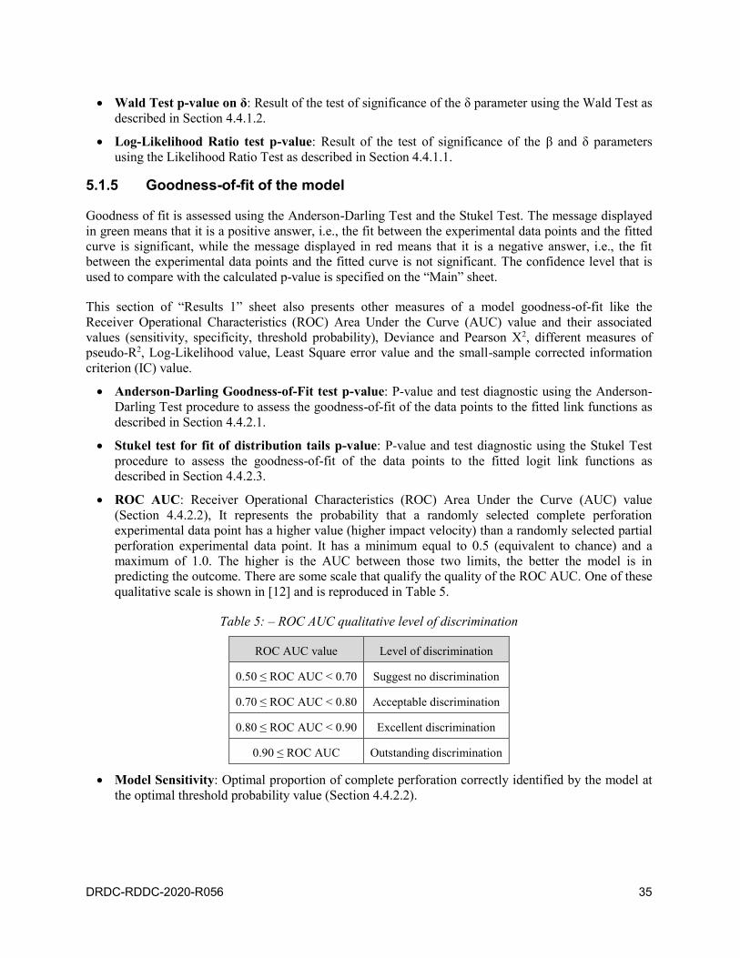
DRDC-RDDC-2020-R056 35
Wald Test p-value on δ: Result of the test of significance of the δ parameter using the Wald Test as
described in Section 4.4.1.2.
Log-Likelihood Ratio test p-value: Result of the test of significance of the β and δ parameters
using the Likelihood Ratio Test as described in Section 4.4.1.1.
5.1.5 Goodness-of-fit of the model
Goodness of fit is assessed using the Anderson-Darling Test and the Stukel Test. The message displayed
in green means that it is a positive answer, i.e., the fit between the experimental data points and the fitted
curve is significant, while the message displayed in red means that it is a negative answer, i.e., the fit
between the experimental data points and the fitted curve is not significant. The confidence level that is
used to compare with the calculated p-value is specified on the “Main” sheet.
This section of “Results 1” sheet also presents other measures of a model goodness-of-fit like the
Receiver Operational Characteristics (ROC) Area Under the Curve (AUC) value and their associated
values (sensitivity, specificity, threshold probability), Deviance and Pearson X2, different measures of
pseudo-R2, Log-Likelihood value, Least Square error value and the small-sample corrected information
criterion (IC) value.
Anderson-Darling Goodness-of-Fit test p-value: P-value and test diagnostic using the Anderson-
Darling Test procedure to assess the goodness-of-fit of the data points to the fitted link functions as
described in Section 4.4.2.1.
Stukel test for fit of distribution tails p-value: P-value and test diagnostic using the Stukel Test
procedure to assess the goodness-of-fit of the data points to the fitted logit link functions as
described in Section 4.4.2.3.
ROC AUC: Receiver Operational Characteristics (ROC) Area Under the Curve (AUC) value
(Section 4.4.2.2), It represents the probability that a randomly selected complete perforation
experimental data point has a higher value (higher impact velocity) than a randomly selected partial
perforation experimental data point. It has a minimum equal to 0.5 (equivalent to chance) and a
maximum of 1.0. The higher is the AUC between those two limits, the better the model is in
predicting the outcome. There are some scale that qualify the quality of the ROC AUC. One of these
qualitative scale is shown in [12] and is reproduced in Table 5.
Table 5: – ROC AUC qualitative level of discrimination
ROC AUC value Level of discrimination
0.50 ≤ ROC AUC < 0.70 Suggest no discrimination
0.70 ≤ ROC AUC < 0.80 Acceptable discrimination
0.80 ≤ ROC AUC < 0.90 Excellent discrimination
0.90 ≤ ROC AUC Outstanding discrimination
Model Sensitivity: Optimal proportion of complete perforation correctly identified by the model at
the optimal threshold probability value (Section 4.4.2.2).
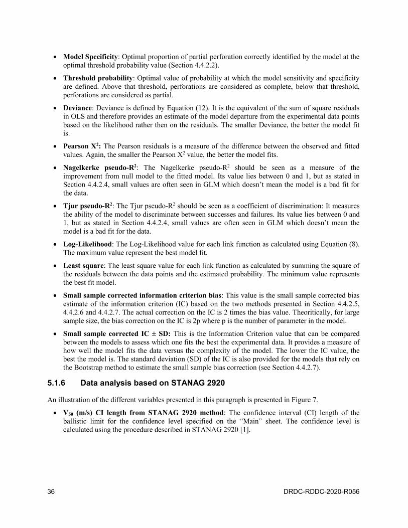
36 DRDC-RDDC-2020-R056
Model Specificity: Optimal proportion of partial perforation correctly identified by the model at the
optimal threshold probability value (Section 4.4.2.2).
Threshold probability: Optimal value of probability at which the model sensitivity and specificity
are defined. Above that threshold, perforations are considered as complete, below that threshold,
perforations are considered as partial.
Deviance: Deviance is defined by Equation (12). It is the equivalent of the sum of square residuals
in OLS and therefore provides an estimate of the model departure from the experimental data points
based on the likelihood rather then on the residuals. The smaller Deviance, the better the model fit
is.
Pearson X2: The Pearson residuals is a measure of the difference between the observed and fitted
values. Again, the smaller the Pearson X2 value, the better the model fits.
Nagelkerke pseudo-R2: The Nagelkerke pseudo-R2 should be seen as a measure of the
improvement from null model to the fitted model. Its value lies between 0 and 1, but as stated in
Section 4.4.2.4, small values are often seen in GLM which doesn’t mean the model is a bad fit for
the data.
Tjur pseudo-R2: The Tjur pseudo-R2 should be seen as a coefficient of discrimination: It measures
the ability of the model to discriminate between successes and failures. Its value lies between 0 and
1, but as stated in Section 4.4.2.4, small values are often seen in GLM which doesn’t mean the
model is a bad fit for the data.
Log-Likelihood: The Log-Likelihood value for each link function as calculated using Equation (8).
The maximum value represent the best model fit.
Least square: The least square value for each link function as calculated by summing the square of
the residuals between the data points and the estimated probability. The minimum value represents
the best fit model.
Small sample corrected information criterion bias: This value is the small sample corrected bias
estimate of the information criterion (IC) based on the two methods presented in Section 4.4.2.5,
4.4.2.6 and 4.4.2.7. The actual correction on the IC is 2 times the bias value. Theoritically, for large
sample size, the bias correction on the IC is 2p where p is the number of parameter in the model.
Small sample corrected IC ± SD: This is the Information Criterion value that can be compared
between the models to assess which one fits the best the experimental data. It provides a measure of
how well the model fits the data versus the complexity of the model. The lower the IC value, the
best the model is. The standard deviation (SD) of the IC is also provided for the models that rely on
the Bootstrap method to estimate the small sample bias correction (see Section 4.4.2.7).
5.1.6 Data analysis based on STANAG 2920
An illustration of the different variables presented in this paragraph is presented in Figure 7.
V50 (m/s) CI length from STANAG 2920 method: The confidence interval (CI) length of the
ballistic limit for the confidence level specified on the “Main” sheet. The confidence level is
calculated using the procedure described in STANAG 2920 [1].
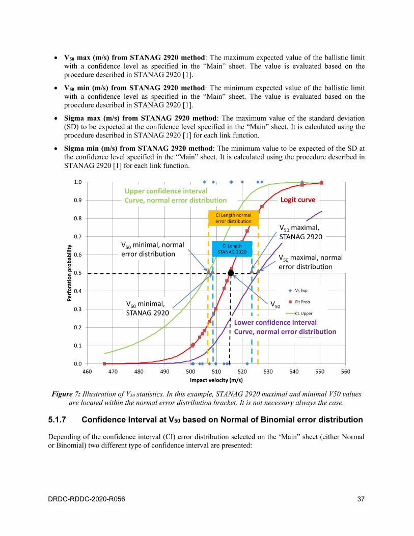
DRDC-RDDC-2020-R056 37
V50 max (m/s) from STANAG 2920 method: The maximum expected value of the ballistic limit
with a confidence level as specified in the “Main” sheet. The value is evaluated based on the
procedure described in STANAG 2920 [1].
V50 min (m/s) from STANAG 2920 method: The minimum expected value of the ballistic limit
with a confidence level as specified in the “Main” sheet. The value is evaluated based on the
procedure described in STANAG 2920 [1].
Sigma max (m/s) from STANAG 2920 method: The maximum value of the standard deviation
(SD) to be expected at the confidence level specified in the “Main” sheet. It is calculated using the
procedure described in STANAG 2920 [1] for each link function.
Sigma min (m/s) from STANAG 2920 method: The minimum value to be expected of the SD at
the confidence level specified in the “Main” sheet. It is calculated using the procedure described in
STANAG 2920 [1] for each link function.
0.0
0.1
0.2
0.3
0.4
0.5
0.6
0.7
0.8
0.9
1.0
460 470 480 490 500 510 520 530 540 550 560
Pe
rfo
rati
on
pro
bab
ility
Impact velocity (m/s)
Vs Exp.
Fit Prob
CL Upper
CL Lower
Fitted curve
V50
V50 maximal, normalerror distribution
V50 minimal, normalerror distribution
V50 maximal, STANAG 2920
V50 minimal, STANAG 2920
Upper confidence intervalCurve, normal error distribution Logit curve
Lower confidence intervalCurve, normal error distribution
CI Length STANAG 2920
CI Length normal error distribution
Figure 7: Illustration of V50 statistics. In this example, STANAG 2920 maximal and minimal V50 values
are located within the normal error distribution bracket. It is not necessary always the case.
5.1.7 Confidence Interval at V50 based on Normal of Binomial error distribution
Depending of the confidence interval (CI) error distribution selected on the ‘Main” sheet (either Normal
or Binomial) two different type of confidence interval are presented:
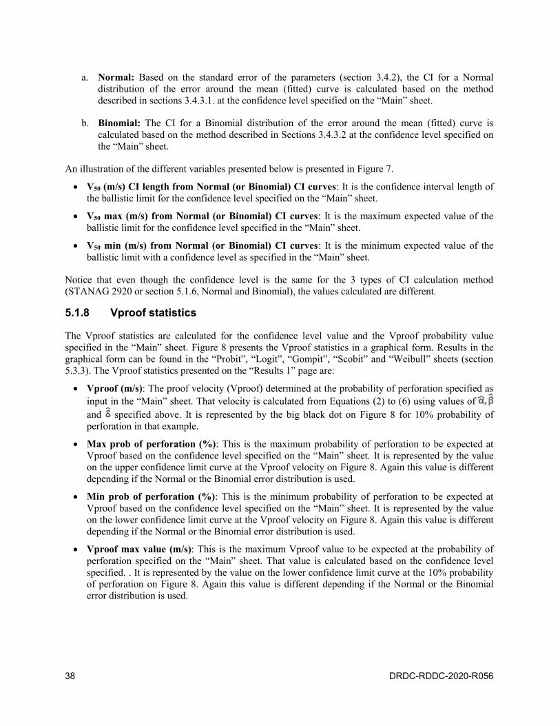
38 DRDC-RDDC-2020-R056
a. Normal: Based on the standard error of the parameters (section 3.4.2), the CI for a Normal
distribution of the error around the mean (fitted) curve is calculated based on the method
described in sections 3.4.3.1. at the confidence level specified on the “Main” sheet.
b. Binomial: The CI for a Binomial distribution of the error around the mean (fitted) curve is
calculated based on the method described in Sections 3.4.3.2 at the confidence level specified on
the “Main” sheet.
An illustration of the different variables presented below is presented in Figure 7.
V50 (m/s) CI length from Normal (or Binomial) CI curves: It is the confidence interval length of
the ballistic limit for the confidence level specified on the “Main” sheet.
V50 max (m/s) from Normal (or Binomial) CI curves: It is the maximum expected value of the
ballistic limit for the confidence level specified in the “Main” sheet.
V50 min (m/s) from Normal (or Binomial) CI curves: It is the minimum expected value of the
ballistic limit with a confidence level as specified in the “Main” sheet.
Notice that even though the confidence level is the same for the 3 types of CI calculation method
(STANAG 2920 or section 5.1.6, Normal and Binomial), the values calculated are different.
5.1.8 Vproof statistics
The Vproof statistics are calculated for the confidence level value and the Vproof probability value
specified in the “Main” sheet. Figure 8 presents the Vproof statistics in a graphical form. Results in the
graphical form can be found in the “Probit”, “Logit”, “Gompit”, “Scobit” and “Weibull” sheets (section
5.3.3). The Vproof statistics presented on the “Results 1” page are:
Vproof (m/s): The proof velocity (Vproof) determined at the probability of perforation specified as
input in the “Main” sheet. That velocity is calculated from Equations (2) to (6) using values of
and specified above. It is represented by the big black dot on Figure 8 for 10% probability of
perforation in that example.
Max prob of perforation (%): This is the maximum probability of perforation to be expected at
Vproof based on the confidence level specified on the “Main” sheet. It is represented by the value
on the upper confidence limit curve at the Vproof velocity on Figure 8. Again this value is different
depending if the Normal or the Binomial error distribution is used.
Min prob of perforation (%): This is the minimum probability of perforation to be expected at
Vproof based on the confidence level specified on the “Main” sheet. It is represented by the value
on the lower confidence limit curve at the Vproof velocity on Figure 8. Again this value is different
depending if the Normal or the Binomial error distribution is used.
Vproof max value (m/s): This is the maximum Vproof value to be expected at the probability of
perforation specified on the “Main” sheet. That value is calculated based on the confidence level
specified. . It is represented by the value on the lower confidence limit curve at the 10% probability
of perforation on Figure 8. Again this value is different depending if the Normal or the Binomial
error distribution is used.
DRDC-RDDC-2020-R056 39
Vproof min value (m/s): This is the minimum Vproof value to be expected at the probability of
perforation specified on the “Main” sheet. That value is calculated based on the confidence level
specified. Again this value is different depending if the Normal or the Binomial error distribution is
used.
10% probability of perforation
Vproof
Max prob of perforation
Min prob of perforation
Upper confidence limit
Lowerconfidence limit
Vproofmax value
Cumulative normal curve
Figure 8: Schematic illustrating Vproof statistics with an example for 10% probability of perforation.
The fitted cumulative function is presented in red, the lower confidence limit is presented in purple and
the upper confidence limit is presented in green.
5.2 Experimental data points and confidence limit curves (“Results 2” sheet)
On the “Results 2” Sheet, the experimental data points and confidence limit curves can be found. It
consists of a serie of six tables. The first table contains the ordered experimental data. The second, third,
fourth, fifth and sixth tables contain the fitted probability values and the upper and lower confidence limit
curves for each of the link function (Logit, Probit, Scobit, Gompit and Weibull). The confidence limit
curves are calculated based on the selected confidence interval error distribution and the confidence level
for the error distribution (both specified on the “Main” sheet) and they are compatible with the values
described in section 5.1.7 (Confidence Interval at V50 based on Normal of Binomial error distribution).
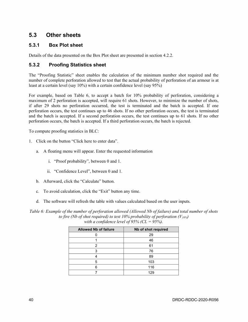
40 DRDC-RDDC-2020-R056
5.3 Other sheets
5.3.1 Box Plot sheet
Details of the data presented on the Box Plot sheet are presented in section 4.2.2.
5.3.2 Proofing Statistics sheet
The “Proofing Statistic” sheet enables the calculation of the minimum number shot required and the
number of complete perforation allowed to test that the actual probability of perforation of an armour is at
least at a certain level (say 10%) with a certain confidence level (say 95%)
For example, based on Table 6, to accept a batch for 10% probability of perforation, considering a
maximum of 2 perforation is accepted, will require 61 shots. However, to minimize the number of shots,
if after 29 shots no perforation occurred, the test is terminated and the batch is accepted. If one
perforation occurs, the test continues up to 46 shots. If no other perforation occurs, the test is terminated
and the batch is accepted. If a second perforation occurs, the test continues up to 61 shots. If no other
perforation occurs, the batch is accepted. If a third perforation occurs, the batch is rejected.
To compute proofing statistics in BLC:
1. Click on the button “Click here to enter data”.
a. A floating menu will appear. Enter the requested information
i. “Proof probability”, between 0 and 1.
ii. “Confidence Level”, between 0 and 1.
b. Afterward, click the “Calculate” button.
c. To avoid calculation, click the “Exit” button any time.
d. The software will refresh the table with values calculated based on the user inputs.
Table 6: Example of the number of perforation allowed (Allowed Nb of failure) and total number of shots
to fire (Nb of shot required) to test 10% probability of perforation (V10%)
with a confidence level of 95% (CL = 95%).
Allowed Nb of failure Nb of shot required
0 29
1 46
2 61
3 76
4 89
5 103
6 116
7 129

DRDC-RDDC-2020-R056 41
Allowed Nb of failure Nb of shot required
8 142
9 154
10 167
5.3.3 Graphical output sheets
The 5 graphical output sheets are “Probit”, “Logit”, “Gompit”, “Scobit” and “Weibull” sheets. These
5 sheets present the graphical representation of the experimental data, the fitted curve using the ML fitting
process and the confidence limit curves based on the error distribution shape and the confidence level for
the error distribution values provided in the “Main” sheet.
0.0
0.1
0.2
0.3
0.4
0.5
0.6
0.7
0.8
0.9
1.0
460 470 480 490 500 510 520 530 540 550 560
Pe
rfo
rati
on
pro
bab
ility
Impact velocity (m/s)
Vs Exp.
Fit Prob
CL Upper
CL Lower
Fitted curve
0.0
0.1
0.2
0.3
0.4
0.5
0.6
0.7
0.8
0.9
1.0
460 470 480 490 500 510 520 530 540 550 560
Pe
rfo
rati
on
pro
bab
ility
Impact velocity (m/s)
Vs Exp.
Fit Prob
CL Upper
CL Lower
Fitted curve
Figure 9: Example of perforation probability fitted curve for normal error (left) and binomial error
(right) distribution for 95% confidence level.
As example, Figure 9 presents the probability of perforation for the Logit link function with the normal
error distribution shape and the binomial error distribution shape. Experimental data points are presented
in blue of the 0.0 and 1.0 probability of perforation axis, the fitted data points corresponding to the
experimental data points are presented as red squares, the fitted curve is the continuous line in red and
finally the upper and lower confidence limit curves are represented by continuous green and purple curves
respectively. The processes to calculate the confidence limits is explained in Section 3.4.3.
5.3.4 ROC sheet
Receiver Operating Characteristcs curves for each of the link function are presented on the ROC sheet.
Details of what is an ROC curve and its signification can be found in Section 4.4.2.2.
42 DRDC-RDDC-2020-R056
6 Data analysis example
6.1 General
This section provides a description of the proposed process for the analysis of ballistic data. It is divided
in two parts: The first concerns the selection of the best model and how to determine which models are
valid for further analysis, while the second details where the data for ballistic data analysis can be found
in BLC. Both processes are illustrated by an example.
6.2 Determination of the correct model
This section deals with the question: How to determine which model is correct? Keeping in mind George
Box quotation: "The most that can be expected from any model is that it can supply a useful
approximation to reality: All models are wrong; some models are useful", this question then become
which model is closer to reality? To answer that question, guidelines on how to analyse data calculated by
BLC are presented. Then, an example of typical output is presented and guidelines mentionned above are
applied.
6.2.1 Guidelines
Various output on the “Results 1” sheet can help diagnose which model better represent the data:
1. The first thing is to verify if the calculated parameters ( and ) are significant. To verify that
point, the Wald test and Likelihood Ratio results can be analysed.
a. Each of the 2 or 3 parameters have to be significant using the Wald Test (that is, the message
“Reject that (α or β or δ) is null” appears in green). Remember that the Wald test should be
considered as a conservative test, that is: if the Wald test rejects the null hypothesis, then the
tested parameter is most likely significant, because as mentioned in [12], it often fails to reject the
null hypothesis even though the parameter is significant.
b. Similarly, the Likelihood Ratio tests compares the full model to the constant only ( parameter
only) model. Again, if the message “Reject that α, β and δ is null” appears in green, then this
means that β (for 2 parameters link functions) or β and δ (for 3 parameters link functions) are
significant.
2. The other thing to verify is the goodness-of-fit of the model relative to the data. This can be verified
using the Anderson-Darling (AD) test, and the ROC.
a. The ROC AUC has to be as close as possible to 1.0. Use of the BLC until now have very often
shown that the value of the ROC AUC is the same for all link function. The model should at least
have an ROC AUC value above 0.70, which represents an acceptable discrimination (Table 5).

DRDC-RDDC-2020-R056 43
b. Because they represent the proportion of complete and partiel perforation correctly identified by
the model, sensitivity and specificity of the model has to be as close as possible to 1.
c. The use of the AD test to assess if the experimental data sample is a good fit to the ML fitted link
function can be done keeping in mind, as mentionned in Section 4.4.2.1, that:
i. Sample sizes above 50 are required to reach power levels above 80%.
ii. For lower sample size, the increase of the allowable Type I error level results in higher
power level for the same sample size. As a result, it is advisable to accept higher Type I
error (15 to 20%) in order to reach acceptable Type II error rates for the typical types of
sample size used in ballistic studies. Therefore, despite the diagnostic provided by BLC, the
actual p-value should be verified and should be above 0.15 to 0.20.
3. The Information Criterion values. The lowest the IC value, the best the model is. Of all the criteria
presented in this section, this is the only one that can be directly compared between the different
models. Different aspects have to be considered when comparing the IC values between models:
a. Use of the BLC until now have shown that the bias correction for sample size as small as 15 can
result in large bias correction which can throw off otherwise promising models.
b. The variance on the IC value for the models which require the Bootstrap method can be quite
large. Therefore, when compared to each others, the difference between the values of IC can be
unsignificant.
c. Reduction of the variance on the bias estimate can be achieved by increasing the number of
experimental data point.
d. A more accurate evaluation of the bias and its variance can be obtained by increasing the total
number of Bootstrap sample from 1000 to say 1000000, but this can only be done at the cost of
very long execution durations.
The selection process to determine the best model can be described in graphical form (Figure 10). A
model that has insignificant parameters is useless, hence the first step is verifying the parameter
significance. The second step is to select the highest ROC AUC value indicating that the selected model
has the highest predictive capability. Finally, the IC has to be verified. It is a combination of the lowest
Log likelihood value and the lowest model complexity. It has to be as low as possible.
For some reasons, it is possible that only one specific model needs to be used (for example, because it is
necessary to follow the STANAG 2920 or the NIJ 0101.06 standard). In this case, only the validity of the
model has to be verified and therefore only the parameter significance and the ROC AUC (higher than
0.70) needs to be checked (Figure 10).
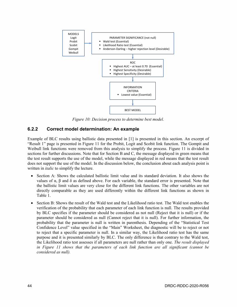
44 DRDC-RDDC-2020-R056
PARAMETER SIGNIFICANCE (not null) Wald test (Essential) Likelihood Ratio test (Essential) Anderson-Darling – higher rejection level (Desirable)
ROC Highest AUC – at least 0.70 (Essential) Highest Sensitivity (Desirable) Highest Specificity (Desirable)
INFORMATIONCRITERIA
Lowest value (Essential)
MODELSLogit
ProbitScobit
GompitWeibull
BEST MODEL
Figure 10: Decision process to determine best model.
6.2.2 Correct model determination: An example
Example of BLC results using ballistic data presented in [1] is presented in this section. An excerpt of
“Result 1” page is presented in Figure 11 for the Probit, Logit and Scobit link function. The Gompit and
Weibull link functions were removed from this analysis to simplify the process. Figure 11 is divided in
sections for further discussions. Note that for Section B and C, the message displayed in green means that
the test result supports the use of the model, while the message displayed in red means that the test result
does not support the use of the model. In the discussion below, the conclusion about each analysis point is
written in italic to simplify the lecture.
Section A: Shows the calculated ballistic limit value and its standard deviation. It also shows the
values of α, β and δ as defined above. For each variable, the standard error is presented. Note that
the ballistic limit values are very close for the different link functions. The other variables are not
directly comparable as they are used differently within the different link functions as shown in
Table 1.
Section B: Shows the result of the Wald test and the Likelihood ratio test. The Wald test enables the
verification of the probability that each parameter of each link function is null. The results provided
by BLC specifies if the parameter should be considered as not null (Reject that it is null) or if the
parameter should be considered as null (Cannot reject that it is null). For further information, the
probability that the parameter is null is written in parenthesis. Depending of the “Statistical Test
Confidence Level” value specified in the “Main” Worksheet, the diagnostic will be to reject or not
to reject that a specific parameter is null. In a similar way, the Likelihood ratio test has the same
purpose and it is presented similarly by BLC. The only difference is that contrary to the Wald test,
the Likelihood ratio test assesses if all parameters are null rather than only one. The result displayed
in Figure 11 shows that the parameters of each link function are all significant (cannot be
considered as null).
DRDC-RDDC-2020-R056 45
Section C: Shows the result of the Anderson-Darling test and the Stukel test. The Anderson-Darling
test compares the experimental distribution of partial-complete penetrations to the fitted curve and
assesses if they correspond. It therefore assesses if the experimental data corresponds to the best
fitted link function. The results provided by BLC specifies if we can or cannot reject that the
experimental data corresponds to a specific link function. Again the probability values is specified in
parenthesis. The Stukel test was designed for the Logit link function and verifies if its parameters
are significant (not null). This is done by enhancing the capability of the Logit function at its tails
and therefore provides information on the tail of the fitted Logit function. The result displayed in
Figure 11 shows that the experimental data corresponds to the Logit and Probit fitted function. It
also shows that the experimental data do not corresponds well to the fitted Scobit function. Finally,
the Stukel test shows that the experimental data are poorly modeled by the tails of the Logit
function.
Section D: Shows the model’s AUC, sensitivity and specificity. The closer the AUC is from 1.0, the
better the model is. Each model sensitivity (proportion of complete penetration correctly predicted
by the model) and specificity (proportion of partial penetration correctly predicted by the model)
also needs to be as close to 1.0 as possible. The result displayed in Figure 11 shows that the 3
models are equivalent in terms of AUC, sensitivity and specificity. With a AUC of 85.86%, the
models are showing excellent discrimination (Table 5).
Section E: Shows the Tjur and Nagelkerke pseudo-R2 values for the different models. The value has
to be as close as possible to 1.0. Nagelkerke pseudo-R2 measures the improvement from null model
to the fitted model. The Tjur pseudo-R2 should be seen as a coefficient of discrimination and
therefore measures the ability of the model to discriminate between successes and failures. The
result displayed in Figure 11 shows that the Scobit model has the highest values of pseudo-R2.
Section F: Shows the Log Likelihood value and the Least-square value for the different models.
Remember that the model which has the highest likelihood (highest possible value of likelihood is
1.0) corresponds to the model that has the Log likelihood value closest to 0 (log(1) = 0). The result
displayed in Figure 11 shows that the model that has the Log likelihood value closest to 0 is the
Scobit model whereas the model that has the lowest least-square value is the Probit model.
Section G: Shows the Information Criterion for each model. The IC accounts for how well the
model fits the data and also accounts for the complexity of the model. It is the summation of the Log
likelihood value and the number of parameters (Equation (23)). This is the only criteria that enables
the comparison between the different models. The model with the lowest IC values is the best
model. The result displayed in Figure 11 shows that the Probit is the best of the 3 models because it
fits well the data and because of his simplicity. The Scobit model has a lower Log likelihood value,
therefore better fit the data, but it is more complex than the Probit model.
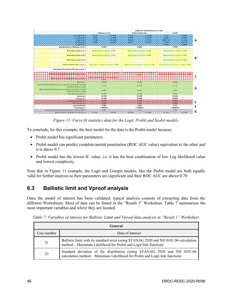
46 DRDC-RDDC-2020-R056
± 4.0419 516.06 ± 1394.2220
± 4.5551 1164816.3056 ± 1394.8439
± 8.4774 0.9996 ± 0.0012
± 0.0164 0.0000 ± 0.0000
128917.4142 ± 64342.6965
± 9.0753 32.4126 ± 5.7077
Reject that α is null (p = 0.000)
Reject that β is null (p = 0.000)
0.8586
0.7778
0.9091
0.4800
-9.276
1.8615E-01
6.930
18.5521
Weibull
Cannot reject that α is null (p = 1.000)
Reject that β is null (p = 0.000)
Reject that δ is null (p = 0.023)
Reject that α, β and δ are null (p = 0.005)
Reject that distribution is Weibull (p = 0.012)Reject that distribution is Gompit (p = 0.013)
Reject that α and β are null (p = 0.005)
0.4314
0.3711
16.2410
0.4837
Figure 11: Curve fit statistics data for the Logit, Probit and Scobit models.
To conclude, for this example, the best model for the data is the Probit model because:
Probit model has significant parameters
Probit model can predict complete/partial penetration (ROC AUC value) equivalent to the other and
it is above 0.7.
Probit model has the lowest IC value, i.e. it has the best combination of low Log likelihood value
and lowest complexity.
Note that in Figure 11 example, the Logit and Gompit models, like the Probit model are both equally
valid for further analysis as their parameters are significant and their ROC AUC are above 0.70.
6.3 Ballistic limit and Vproof analysis
Once the model of interest has been validated, typical analysis consists of extracting data from the
different Worksheets. Most of data can be found in the “Result 1” Worksheet. Table 7 summarises the
most important variables and where they are located.
Table 7: Variables of interest for Ballistic Limit and Vproof data analysis in “Result 1” Worksheet.
General
Line number Data of interest
21 Ballistic limit with its standard error (using STANAG 2920 and NIJ 0101.06 calculation
method – Maximum Likelihood for Probit and Logit link function)
22 Standard deviation of the distribution (using STANAG 2920 and NIJ 0101.06
calculation method – Maximum Likelihood for Probit and Logit link function)
V50 ± SE (m/s) = 515.25 ± 3.8825 515.20 ± 3.8295 517.24 ± 0.7923
σ ± SE (m/s) = 6.6496 ± 3.3908 10.9791 ± 5.3795 0.0841 ± 0.0001
α ± SE (m/s) = -77.4866 ± 24.5426 -46.9257 ± 19.3767 -6260.7103 ± 9.4536
β ± SE (m/s) = 0.1504 ± 0.0478 0.0911 ± 0.0378 11.8953 ± 0.0179
δ ± SE (m/s) = 0.0064 ± 0.0022
Standard Error of Estimate at V50 =
Wald test p-value on α =
Wald test p-value on β =
Wald test p-value on δ =
Likelihood Ratio test p-value =
Osius-Rojek Goodness-of-Fit test p-value =
Anderson-Darling Goodness-of-Fit test p-value =
Stukel test for fit of distribution tails p-value =
ROC AUC =
Model Sensitivity (Proportion of complete perforation correctly
identified by the model)
Model Specificity (Proportion of partial perforation correctly
identified by the model)
Threshold probability =
Deviance =
Pearson X2 =
Nagelkerke pseudo R2 =
Tjur pseudo R2 =
Log Likelihood =
Least square =
Small Sample Corrected Information Criterion Bias =
Small Sample Corrected IC ± SD (m/s) = 23.5451 ± 0.0000 23.0840 ± 0.0000 24.1334 ± 2.7488
18.6390
0.4309
0.8586
16.2809
0.4799
0.3669
0.8586
2.223
1.8566E-011.7683E-01
0.8586
0.7778
0.9091
0.5100
1.7656E-01
0.7778
0.9091
0.5100
18.7279
16.3956
0.4761
0.3636
-9.364
Logit (NIJ 0101.06)
0.4202
Reject that α is null (p = 0.008)
Reject that β is null (p = 0.008)
0.4205
Probit (STANAG 2920)
0.9091
Reject that δ is null (p = 0.002)
Scobit
Reject that α is null (p = 0.001)
Reject that β is null (p = 0.000)
Reject that distribution is Scobit (p = 0.000)
Reject that α is null (p = 0.000)
Reject that α, β and δ are null (p = 0.004)
Cannot reject that distribution is Probit (p =
0.222)
Reject that α and β are null (p = 0.005)
Reject that β is null (p = 0.001)
Cannot reject that distribution is Logit (p =
0.382)
Logit model tails do not fit the data (p =
0.001)
Reject that α and β are null (p = 0.005)
CURVE FIT STATISTICS for Cl = 95%
-9.320
2.409
0.7778
0.4400
18.2416
15.8247
0.4968
0.3830
-9.121
2.946
A
B
C
D
E
G
F
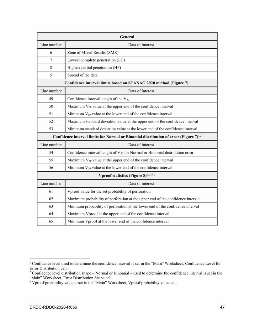
DRDC-RDDC-2020-R056 47
General
Line number Data of interest
6 Zone of Mixed Results (ZMR)
7 Lowest complete penetration (LC)
8 Highest partial penetration (HP)
5 Spread of the data
Confidence interval limits based on STANAG 2920 method (Figure 7)1
Line number Data of interest
49 Confidence interval length of the V50
50 Maximum V50 value at the upper end of the confidence interval
51 Minimum V50 value at the lower end of the confidence interval
52 Maximum standard deviation value at the upper end of the confidence interval
53 Minimum standard deviation value at the lower end of the confidence interval
Confidence interval limits for Normal or Binomial distribution of error (Figure 7)1,2
Line number Data of interest
54 Confidence interval length of V50 for Normal or Binomial distribution error
55 Maximum V50 value at the upper end of the confidence interval
56 Minimum V50 value at the lower end of the confidence interval
Vproof statistics (Figure 8)1, 2 & 3
Line number Data of interest
61 Vproof value for the set probability of perforation
62 Maximum probability of perforation at the upper end of the confidence interval
63 Minimum probability of perforation at the lower end of the confidence interval
64 Maximum Vproof at the upper end of the confidence interval
65 Minimum Vproof at the lower end of the confidence interval
1 Confidence level used to determine the confidence interval is set in the “Main” Worksheet, Confidence Level for
Error Distribution cell. 2 Confidence level distribution shape – Normal or Binomial – used to determine the confidence interval is set in the
“Main” Worksheet, Error Distribution Shape cell. 3 Vproof probability value is set in the “Main” Worksheet, Vproof probability value cell.

48 DRDC-RDDC-2020-R056
7 Conclusion
This document provides scientific information on the mathematical and statistical methods used by the
BLC (Ballictic Limit Calculator) Beta version 2 program to generate ballistic limit and Vproof data and
their related statistics based on experimental ballistic data.
The BLC software enables the analysis of ballistic data using 5 different statistical models (namely, the
Probit, Logit, Gompit, Scobit and Weibull models) that, at least for the Probit and Logit models, follow
the data analysis procedures of STANAG 2920 and NIJ 0101.06 standards. In addition, different
statistical measures and statistical tests are presented along with their limitations and details on their
meaning. This enables the BLC user to have a clear understanding of the significance and the goodness of
fit of the different models. In addition, typical data analysis process is presented through an example.
This document is also the user manual of the BLC Beta version 2 program. As such, this document
provides details on the nature and meaning of input and output information and presents its different
features.
DRDC-RDDC-2020-R056 49
References
[1] AEP 2920 – Procedures for the Evaluation and Classification of Personal Armour, Bullet and
Fragmentation Threats, Edition A, Version 1, 22 June 2015, NATO Standardization Office, Brussels.
[2] STANAG 2920 – Classification of Personal Armour (EDITION 3), 22 June 2015, NATO
Standardization Office, Brussels.
[3] NIJ Standard-0101.06 – Ballistic Resistance of Body Armour, July 2008, U.S. Department of Justice,
Office of Justice Programs, National Institute of Justice.
[4] Nagler, J., Scobit: An Alternative Estimator to Logit and Probit, Americam Journal of Political
Science, Vol. 38, No. 1, February 1994, pp 230–255.
[5] Brathwaite, T. and Walker, J.L., Asymmetric, closed-form, finite-parameter models of multinomial
choice, Journal of Choice Modelling (2017), http://dx.doi.org/10.1016/j.jocm.2018.01.002
[6] Mauchant, D., Rice, K.D., Riley, M.A., Leber, D., Samarov, D., and Forster, A.L., Analysis of Three
Different Regression Models to Estimate the Ballistic Performance of New and Environmentally
Conditioned Body Armor, U.S. Department of Commerce, National Institute of Standards and
Technology, NISTIR 7760, February 2011.
[7] Nelder, J.A. and Mead, R.A., A simplex method for function minimization. Computer Journal, Vol. 7,
308–313, 1965.
[8] Williams, R., Maximum Likelihood Estimation, University of Notre-Dame,
http://www3.nd.edu/~rwilliam/, Last revised January 14, 2016, Accessed 13 July 2016.
[9] Watkins, J., Topic 15 – Maximum Likelihood Estimation, University of Arizona,
http://math.arizona.edu/~jwatkins/o-mle.pdf, November 1 and 3 2011. Accessed 13 July 2016.
[10] Genschel, U. and Meeker, W.Q., A Comparison of Maximum Likelihood and Median-Rank
Regression for Weibull Estimation. Quality Engineering, 22 (4), pp. 236–255, 2010.
[11] Nemes, S.,Jonasson, J.M., Genell, A. and Steineck, G., Bias in odds ratios by logistic regression
modelling and sample size, BMC Medical Research Methodology, Vproof. 9, No. 56, 2009.
[12] Hosmer, D.W. and Lemeshow, S., Applied Logistic Regression, Second Edition, Wiley Series on
Probability and Statistics, 2000.
[13] Ku, H.H., Notes on the Use of Propagation of Error Formulas, Journal of Research of the National
Bureau of Standards - C. Engineering and Instrumentation, Vol. 70C, No.4, October–December
1966.
[14] Lorenz, V., Yang, L., Grosse Perdekamp, M., Hertzog, D., Clegg, R., Error Analysis,
https://courses.physics.illinois.edu/phys403/sp2016/lectures/ErrorAnalysis_Lorenz2016.pdf .
PHYS403 Course lecture, University of Illinois at Urbana, College of Engineering, Spring 2016.
50 DRDC-RDDC-2020-R056
[15] Heo, J.H., Salas, J.D, Kim, K.D., Estimation of Confidence Intervals of Quantiles for the Weibull
Distribution, Stochastic Environmental Research and Risk Assessment, Vol. 15, 2001, pp 284–309.
[16] NIST/SEMATECH, e-Handbook of Statistical Methods: Measures of Skewness and Kurtosis,
https://www.itl.nist.gov/div898/handbook/eda/section3/eda35b.htm ,
[17] Bulmer, M.G., Principles of Statistics,. The M. I. T. Press, 1965, 214 pages.
[18] Williams, R., Logistic Regression, Part III: Hypothesis Testing, Comparisons to OLS, University of
Notre Dame, http://www3.nd.edu/~rwilliam/ , Last revised February 22, 2015.
[19] DeCook, R., 22s:152 Applied Linear Regression: Ch. 14 (sec. 1) and Ch. 15 (sec. 1 & 4), Logistic
Regression, Department of Statistics and Actuarial Science, University of Iowa,
http://homepage.stat.uiowa.edu/~rdecook/stat3200/notes/LogReg_part2_4pp.pdf , STAT3200
course notes, July 2011.
[20] Rukhin, A., Soto, J., Nechvatal, J., Smid, M., Barker, E., Leigh,S., Levenson, M., Vangel, M.,
Banks, D., Heckert, A., Dray,J. and Vo, S., A Statistical Test Suite for Random and Pseudorandom
Number Generators for Cryptographic Applications, US Department of Commerce, National
Institute of Standards and Technology, NIST Special Publication 800-22, Revision 1a, 2010.
[21] Rukhin, A.L., Statistical Testing of Randomness : New and Old Procdures, Appeared as Chapter 3
in Randomness Through Computation by Zenil, H. ed., World Scientific, pp 33-51, 2011.
[22] Pennsylvania State University, Department of Statistics Online Programs, Stat 414/415, Lesson 49,
The Run Test, https://online.stat.psu.edu/stat414/node/329/, 2018.
[23] NCSS Statistical Software, Chapter 256, Analysis of Runs, https://ncss-wpengine.netdna-
ssl.com/wp-content/themes/ncss/pdf/Procedures/NCSS/Analysis_of_Runs.pdf.
[24] Das, U., Dhar, S.S. and Pradhan, V., Corrected likelihood-ratio tests in logistic regression using
small-sample data, Communications in Statistics—Theory and Methods, 2017.
[25] Tanizaki, H., POWER COMPARISON OF EMPIRICAL LIKELIHOOD RATIO TESTS - SMALL
SAMPLE PROPERTIES THROUGH MONTE CARLO STUDIES, Kobe University Economic
Review, Vol. 50, 2004.
[26] Cousineau, D. and Allen, T.A., Likelihood and its use in Parameter Estimation and Model
Comparison, Mesure et évaluation en éducation, Vol 37, No. 3, pp 63–98, 2015.
[27] Stephens, M.A., The Anderson-Darling Statistic, Prepared under Grant DAAG29-77-G-0O31 For
the U.S. Army Research Office, Technical Report No. 39, October 31, 1979.
[28] Razali, N.M. and Wah, Y.B., Power comparisons of Shapiro-Wilk, Kolmogorov-Smirnov, Lilliefors
and Anderson-Darling tests, Journal of Statistical Modeling and Analytics Vol.2 No.1, 21–33, 2011.
DRDC-RDDC-2020-R056 51
[29] Bispo, R., Marques. T.A. and Pestana, D., Statistical power of goodness-of-fit test based on
empirical distribution function for Type-I right censored data, Journal of Statistical Computation
and Simulation, 2011, pp 1–9.
[30] Hosmer, D.W., Hosmer, T., , LE CESSIE, S. and S. Lemeshow, S., A COMPARISON OF
GOODNESS-OF-FIT TESTS FOR THE LOGISTIC REGRESSION MODEL, Statistics in
Medicine, Vol. 16, 1997, pp 965–980.
[31] Mandrekar, J.N., Receiver Operating Characteristic Curve in Diagnostic Test Assessment,
Biostatistics for Clinicians, Journal of Thoracic Oncology, Vol 5, No 9, September 2010.
[32] Hanley, J.A. and Hajian, K.O., Sampling variability of nonparametric estimates of the areas under
receiver operating characteristic curves - An update, Statics in Radiology, Acad Radiol, Vol. 4,
No. 1, January 1997, pp 49-58.
[33] Wonnacott, T.H. and Wonnacott, R.J., Introductory statistics for business and economics, Second
edition, Wiley and Sons Inc., 1997.
[34] Anderson, D.R and Burnham, K.P., Understanding information criteria for selection among capture-
recapture or ring recovery models, Bird Study, 46 (suppl.), 1999, pp S14-21.
[35] Konishi, S. and Kitagawa, G., Information Criteria and Statistical Modeling, Spriger Series in
Statistics, 2008, ISBN: 978-0-387-71886-6.
[36] Takeuchi, K., Distribution of informational statistics and a criterion of model fitting, Suri Kagaku
(Mathematic Sciences), 153, 1976, pp.12–18 (in Japanese)
[37] Akaike, H., A new look at the statistical model identification. IEEE Transactions on Automatic
Control, Vol. 19, No. 6, pp 716–723, 1974.
[38] Imori, S., Yanagihara, H., and Wakaki, H., General Formula of Bias-Corrected AIC in
Generalizwed Linear Models, Scandinavian Journal in Statiststics, Vol. 41,No. 2, pp 535–555,
2014.
DOCUMENT CONTROL DATA *Security markings for the title, authors, abstract and keywords must be entered when the document is sensitive
1. ORIGINATOR (Name and address of the organization preparing the document. A DRDC Centre sponsoring a contractor's report, or tasking agency, is entered in Section 8.)
DRDC – Valcartier Research Centre Defence Research and Development Canada 2459 route de la Bravoure Québec (Québec) G3J 1X5 Canada
2a. SECURITY MARKING (Overall security marking of the document including special supplemental markings if applicable.)
CAN UNCLASSIFIED
2b. CONTROLLED GOODS
NON-CONTROLLED GOODS DMC A
3. TITLE (The document title and sub-title as indicated on the title page.)
Calculation software for ballistic limit and Vproof tests from ballistic tests results (BLC)
4. AUTHORS (Last name, followed by initials – ranks, titles, etc., not to be used)
Bourget, D.; Bolduc, M.
5. DATE OF PUBLICATION (Month and year of publication of document.)
July 2020
6a. NO. OF PAGES
(Total pages, including Annexes, excluding DCD, covering and verso pages.)
60
6b. NO. OF REFS
(Total references cited.)
38
7. DOCUMENT CATEGORY (e.g.,, Scientific Report, Contract Report, Scientific Letter.)
Scientific Report
8. SPONSORING CENTRE (The name and address of the department project office or laboratory sponsoring the research and development.)
DRDC – Valcartier Research Centre Defence Research and Development Canada 2459 route de la Bravoure Québec (Québec) G3J 1X5 Canada
9a. PROJECT OR GRANT NO. (If appropriate, the applicable research and development project or grant number under which the document was written. Please specify whether project or grant.)
02ab - Soldier System Effectiveness (SoSE)
9b. CONTRACT NO. (If appropriate, the applicable number under which the document was written.)
10a. DRDC PUBLICATION NUMBER (The official document number by which the document is identified by the originating activity. This number must be unique to this document.)
DRDC-RDDC-2020-R056
10b. OTHER DOCUMENT NO(s). (Any other numbers which may be assigned this document either by the originator or by the sponsor.)
11a. FUTURE DISTRIBUTION WITHIN CANADA (Approval for further dissemination of the document. Security classification must also be considered.)
Public release
11b. FUTURE DISTRIBUTION OUTSIDE CANADA (Approval for further dissemination of the document. Security classification must also be considered.)
12. KEYWORDS, DESCRIPTORS or IDENTIFIERS (Use semi-colon as a delimiter.)
Ballistic Limit; Body armour; Applied Statistics; Personal protective equipment; Personal ballistic protection; Vehicle ballistic protection; Test method
13. ABSTRACT (When available in the document, the French version of the abstract must be included here.)
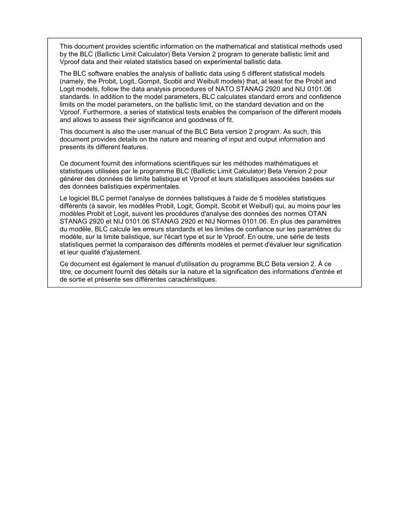
This document provides scientific information on the mathematical and statistical methods used by the BLC (Ballictic Limit Calculator) Beta Version 2 program to generate ballistic limit and Vproof data and their related statistics based on experimental ballistic data.
The BLC software enables the analysis of ballistic data using 5 different statistical models (namely, the Probit, Logit, Gompit, Scobit and Weibull models) that, at least for the Probit and Logit models, follow the data analysis procedures of NATO STANAG 2920 and NIJ 0101.06 standards. In addition to the model parameters, BLC calculates standard errors and confidence limits on the model parameters, on the ballistic limit, on the standard deviation and on the Vproof. Furthermore, a series of statistical tests enables the comparison of the different models and allows to assess their significance and goodness of fit.
This document is also the user manual of the BLC Beta version 2 program. As such, this document provides details on the nature and meaning of input and output information and presents its different features.
Ce document fournit des informations scientifiques sur les méthodes mathématiques et statistiques utilisées par le programme BLC (Ballictic Limit Calculator) Beta Version 2 pour générer des données de limite balistique et Vproof et leurs statistiques associées basées sur des données balistiques expérimentales.
Le logiciel BLC permet l'analyse de données balistiques à l'aide de 5 modèles statistiques différents (à savoir, les modèles Probit, Logit, Gompit, Scobit et Weibull) qui, au moins pour les modèles Probit et Logit, suivent les procédures d'analyse des données des normes OTAN STANAG 2920 et NIJ 0101.06 STANAG 2920 et NIJ Normes 0101.06. En plus des paramètres du modèle, BLC calcule les erreurs standards et les limites de confiance sur les paramètres du modèle, sur la limite balistique, sur l'écart type et sur le Vproof. En outre, une série de tests statistiques permet la comparaison des différents modèles et permet d'évaluer leur signification et leur qualité d'ajustement.
Ce document est également le manuel d'utilisation du programme BLC Beta version 2. À ce titre, ce document fournit des détails sur la nature et la signification des informations d'entrée et de sortie et présente ses différentes caractéristiques.