Calculus 3 Final Exam Review, Spring 2009faculty.madisoncollege.edu/kmirus/20082009C/804233/... · Web viewThus, there is an equivalent of the vertical line test from two dimensions,

Calculus 3 Final Exam Review Sheet Page 1 of 50

Section 11.1: Vector-Valued FunctionsDefinition 1.1: Vector-Valued FunctionA vector-valued function r(t) is a mapping from its domain to its range , so that for each t in D, r(t) = v for exactly one v V3. We can write a vector-valued function as

r(t) = f(t)i + g(t)j + h(t)k,for some scalar functions f, g, and h (called the components of r).

The vector functioncorresponds to the set of parametric equations

Arc length of a curve defined by a vector-valued function r(t) = f(t)i + g(t)j + h(t)k, on an interval t [a, b]:

Parametric equations for an intersection of surfaces:1. Eliminate one variable2. Set another variable to the parameter t.3. Write all variables in terms of t.

Section 11.2: The Calculus of Vector-Valued FunctionsDefinition 2.1: Definition of the Limit of a Vector-Valued FunctionGiven a vector-valued function , we define the limit of as t approaches a as follows:

,

provided all three of the above limits exist. If any one of the limits does not exist, then does not exist.

Definition 2.2: Continuity of a Vector-Valued FunctionWe say the vector-valued function is continuous at t = a if

.

Theorem 2.1: Condition for the Continuity of a Vector-Valued FunctionA vector-valued function is continuous at t = a if and only if all of f, g, and h are continuous at t = a.


Definition 2.3: Definition of the Derivative of a Vector-Valued FunctionThe derivative of the vector-valued function is defined by

at any value of t for which this limit exists. If this limit exists at some value t = a, we say r is differentiable at a.

Theorem 2.2: Derivative of a Vector-Valued Function in Terms of its ComponentsIf , and the components f, g, and h are all differentiable for some value of t,

then r is also differentiable at that value of t and its derivative is given by .

Theorem 2.3: Derivatives of Combinations of Vector-Valued Functions and ScalarsSuppose and are differentiable vector-valued functions, is a differentiable scalar function, and c is a constant. Then

(i)

(ii)

(iii)

(iv)

(v)

Theorem 2.4: Orthogonality of a Constant-Magnitude Vector-Valued Function and Its Derivative

is constant throughout some interval if and only if r(t) and r(t) are orthogonal for all t in that interval.

Definition 2.4: Antiderivative of a Vector-Valued FunctionThe vector-valued function R(t) is an antiderivative of the vector-valued function r(t) if R(t) = r(t).


Definition 2.5: Indefinite Integral of a Vector-Valued FunctionIf R(t) is any antiderivative of the vector-valued function r(t), then the indefinite integral of r(t) is defined as

,

where is an arbitrary constant vector.

Note that this simply corresponds to

Definition 2.6: Definite Integral of a Vector-Valued FunctionFor the vector-valued function , the definite integral of r(t) on the interval [a, b] is defined as:

,

provided all three integrals on the right exist.

Theorem 2.5: Extension of the Fundamental Theorem of Calculus to Vector-Valued FunctionsIf R(t) is an antiderivative of a vector-valued function r(t) on the interval [a, b], then:

.

Section 11.3: Motion in Spacer(t) = v(t), the velocity vector.v(t) = r(t) = a(t), the acceleration vector.Newton’s Second Law states that F = ma.

The general equations for a projectile launched with an initial velocity v0 at an angle of inclination from a location (x0, y0) are:

Time to reach maximum altitude:

Maximum altitude:

Range: Find the time to reach the ground, then use that time to calculate horizontal distance.


Section 11.4: Curvature

Unit Tangent Vector

Curvature

(nearly impossible to calculate this way)

(this is easier to work with, but still pretty hard)

(this is the easiest to compute)

For a 2D plane curve defined by the Cartesian function y = f(x),

For a 2D plane curve defined by the polar function r = f(),

Section 11.5: Tangent and Normal Vectors

The Unit Tangent Vector:

The Principal Unit Normal Vector (Definition 5.1):

(Note: N(t) always points toward the concave side of the curve.)

The Binormal Vector (Definition 5.2)


The osculating circle . . . . has the same curvature as the curve itself at a point P has the same tangent vector as the curve at P (namely, T is tangent to both). has a radius of , called the radius of curvature for the curve at P. is considered the circle of “best fit” for the curve at P.

Tangential and Normal Components of Acceleration

, ,

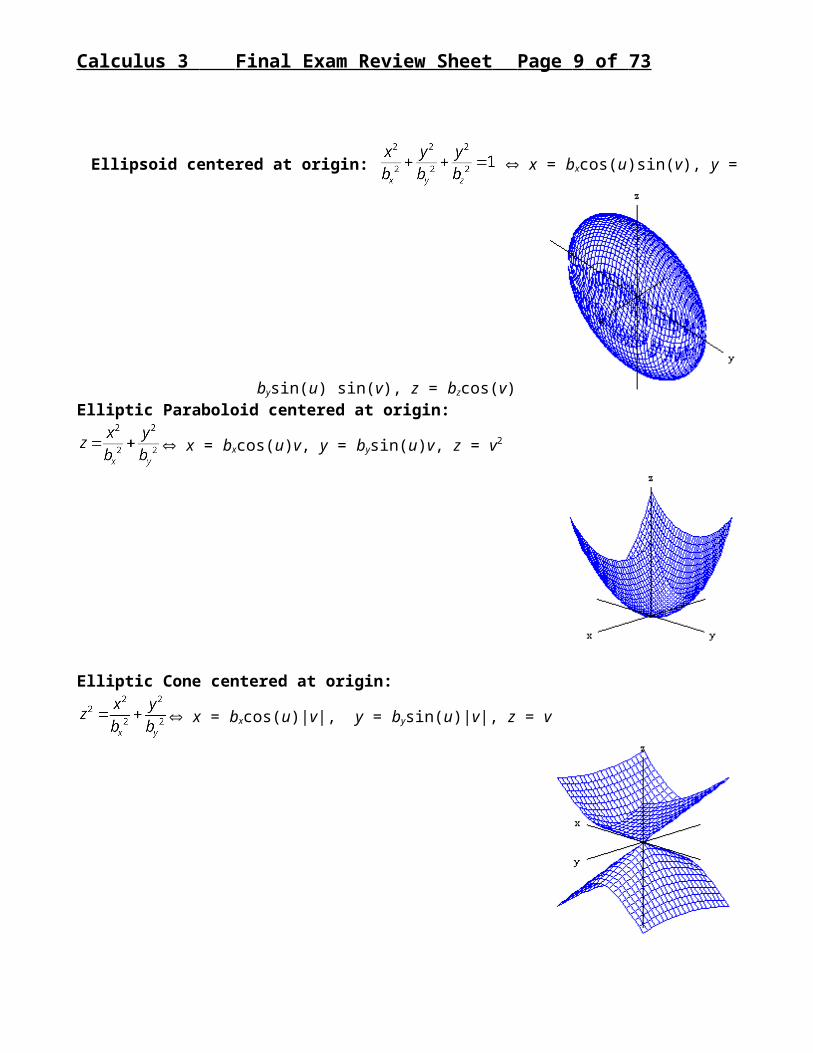
Section 11.6: Parametric SurfacesFor any cylindrical surface formed by “drawing out” a curve defined by x = cos(t), y = sin(t) along the z axis:x = cos(u), y = sin(u), z = v

Sphere centered at origin:x2 + y2 + z2 = r2 x = rcos(u)sin(v), y = rsin(u) sin(v), z = rcos(v)

2 general tricks for converting quadric surface equations to parametric equations:cos2(u) + sin2(u) = 1cosh2(u) – sinh2(u) = 1


Ellipsoid centered at origin: x = bxcos(u)sin(v), y = bysin(u) sin(v), z = bzcos(v)

Elliptic Paraboloid centered at origin:

x = bxcos(u)v, y = bysin(u)v, z = v2

Elliptic Cone centered at origin:

x = bxcos(u)|v|, y = bysin(u)|v|, z = v


Hyperboloid of One Sheet centered at origin:

x = bxcos(u)cosh(v), y = bysin(u)cosh(v), z = bzsinh(v)

Hyperboloid of Two Sheets centered at origin:

x = bxcos(u)sinh(v), y = bysin(u)sinh(v), z = bzcosh(v)


Hyperbolic Paraboloid centered at origin:

x = bxcosh(u)v, y = bysinh(u)v, z = v2

ANDx = bxsinh(u)v, y = bycosh(u)v, z = –v2


Section 12.1: Functions of Several Variables

Definition: Function of Two VariablesA function of two variables is a rule that assigns a single real number to each ordered pair of numbers (x, y) in the domain of the function. We usually write the function as f(x, y) x and y are the independent variables, and are chosen independently of each other If we set z = f(x, y), then z is the dependent variable. The graph of z = f(x, y) will be a surface embedded in a 3D space. For a function f defined on a domain of , we sometimes write to indicate f maps points in two dimensions to real numbers. Not every surface is a function, because by definition, f(x, y) will generate exactly one output for z given any x and y. Thus, there is an equivalent of the vertical line test from two dimensions, which is that a surface in three dimensions is a function if and only if no line parallel to the z-axis intersects the surface more than once. The unit sphere x2 + y2 + z2 = 1 is not a function, but a sphere can be represented using the two functions and . The domain of a function of two variables is the set of all ordered pairs (x, y) for which f(x, y) is defined.

Definition: Function of Three VariablesA function of three variables is a rule that assigns a single real number to each ordered triple of numbers (x, y, z) in the domain of the function. Example: w = f(x, y, z) represents a surface embedded in 4 dimensions…

Contour Plots & Level Curves

Contour plots are 2-dimensional images (drawn in the xy-plane) that provide valuable information about a surface that lives in 3D space. A contour plot consists of a number of level curves for the surface.

Specifically, given a function of two variables, , a level curve is the (2D) graph of the curve , for some constant c. This amounts to intersecting the surface with the place

(a plane perpendicular to the z-axis), and projecting the resulting curve of intersection into the xy-plane. If we generate a number of level curves and plot them all on the same set of axes, the resulting graph is called a contour plot.

The figure on the left below is a graph of the paraboloid . On the right is a contour plot for the surface. The level curves appear to be ellipses, as can easily be confirmed from the equation by setting .


x y

z


Section 12.2: Limits and Continuity

Definition 2.1: Formal Definition of Limit for a Function of Two VariablesLet f be defined on the interior of a circle centered at the point (a, b), except possibly at (a, b) itself.

We say that if for every > 0 there exists a > 0 such that

whenever .

Corollary results for limits of combinations of functions: The limit of a sum or difference is the sum or difference of the limits.

The limit of a product is the product of the limits

The limit of a quotient is the quotient of the limits (except where the denominator is zero)

The limit of a polynomial always exists and is found simply by substitution.

Notes on disproving limits: For a limit to exist, the function must approach that limit for every possible path of (x, y) approaching (a, b). Thus, it is usually very hard to prove a limit exists, and easier to show a limit does not exist. So, if a function f(x, y) approaches L1 as (x, y) approaches (a, b) along a path P1 and f(x, y)

approaches L2 L1 as (x, y) approaches (a, b) along a different path P2, then does

not exist. Some simple paths to try are the lines along x = a, y = b, or any other line through the point.

How can you show a limit does exist? One way is with our old friend the squeeze theorem.Theorem 2.1 (Squeeze Theorem)Suppose that for all (x, y) in the interior of some circle centered at (a, b), except

possibly at (a, b). If , then .


Definition 2.2: Continuity of a Function of Two VariablesSuppose f(x, y) is defined in the interior of a circle centered at the point (a, b). We say that f is

continuous at (a, b) if . If f(x, y) is not continuous at (a, b), then we call (a,

b) a discontinuity of f.

Corollary results for continuity of combinations of functions: The sum or difference of continuous functions is continuous. The product of continuous functions is continuous. The quotient of continuous functions is continuous. (except where the denominator is zero) When discussing the continuity of a composition of functions, one has to be a bit careful:

Theorem 2.2 (Continuity of a Composition of Continuous Functions)Suppose that f(x, y) is continuous at (a, b), and g(x) is continuous at the point f(a, b). Then

is continuous at (a, b).

Extension of the concepts of limit and continuity to functions of three variables:Definition 2.3: Formal Definition of Limit for a Function of Three VariablesLet f(x, y, z) be defined on the interior of a circle centered at the point (a, b, c) except possibly at

(a, b, c) itself. We say that if for every > 0 there exists a > 0 such that

whenever .

Definition 2.4: Continuity of a Function of Three VariablesSuppose f(x, y) is defined in the interior of a sphere centered at the point (a, b, c). We say that f is

continuous at (a, b, c) if . If f(x, y, z) is not continuous at (a, b, c),

then we call (a, b, c) a discontinuity of f.


Section 12.3: Partial DerivativesBig idea: The notion of the derivative of a single-variable function can be extended to a multivariate function if a derivative is taken with respect to one variable while holding the value(s) of the other variable(s) constant. This is called a partial derivative.

Big skill: You should be able to compute first-order and higher-order partial derivatives.

The derivative f (a) of a univariate function f (x) tells us the slope of the tangent line to the

curve y = f(x) at the point (a, f(a)). The partial derivative tells us the slope of the tangent line

to the surface at the point (a, b, f(a, b)) in the plane y = b. The partial derivative

tells us the slope of the tangent line to the surface at the point (a, b, f(a, b)) in the plane x = a.

A graph of and the tangent line to the curve at (1, 2). Note

that and the equation of the tangent line is .


A graph of and the plane y = 1. The plane intersects the surface

along a curve specified by . The

tangent line to the surface at (1, 1, 2) in the plane y = 1 is also shown. Note that in this plane, and the equation of the

tangent line is

For the function ,

.

A graph of and the plane x = 1. The plane intersects the surface

along a curve specified by . The

tangent line to the surface at (1, 1, 2) in the plane x = 1 is also shown. Note that in this plane, and the equation of the

tangent line is

For the function ,

.

Definition 3.1: Partial Derivative

The partial derivative of f(x, y) with respect to x, written as , is defined by

for any values of x and y for which the limit exists.

The partial derivative of f(x, y) with respect to y, written as , is defined by

for any values of x and y for which the limit exists.


Note: To compute a partial derivative in practice, just treat all independent variables as constants except for the variable with respect to which the derivative is being taken.

Various notations for partial derivatives of :

(Likewise for partial derivatives with respect to y)

The expression is a partial differential operator; it indicates to take the partial derivative with

respect to x of whatever expression follows it.

Higher order partial derivatives are partial derivatives of partial derivatives.For a function of two variables, there are four different second-order partial derivatives:

The partial derivative with respect to x of is .

Alternative notations:

The partial derivative with respect to y of is .

Alternative notations:

The partial derivative with respect to x of is .

Alternative notations: . This is a mixed second-order partial

derivative.

The partial derivative with respect to y of is .

Alternative notations: . This is also a mixed second-order

partial derivative.

Theorem 3.1 (Equality of Mixed Second-Order Partial Derivatives)If fxy(x, y) and fyx(x, y) are continuous on an open set containing (a, b), then fxy(x, y) = fyx(x, y).


Section 12.4: Tangent Planes and Linear ApproximationsTheorem 4.1: Equation of a Plane Tangent to a SurfaceSuppose that f(x, y) has continuous first partial derivatives at (a, b). A normal vector to the tangent plane at z = f(x, y) at (a, b) is then <fx(a, b), fy(a, b), -1>. Further, an equation of the tangent plane is given by:

z = f(a, b) + fx(a, b)(x – a) + fy(a, b) (y – b).

Also, the equation of the normal line through the point (a, b, f(a, b)) is given by:x = a + fx(a, b)t, y = b + fy(a, b)t, z = f(a, b) – t.

Just as the tangent line is a linear approximation for a curve near the tangent point, the tangent plane is a linear approximation for a surface near the tangent point. Thus, the linear approximation L(x, y) to a function f(x, y) at the point (a, b) is:

L(x, y) = f(a, b) + fx(a, b)(x – a) + fy(a, b) (y – b).

Increments and Differentials

Defintion: The Differential of a Univariate FunctionLet y = f(x) be a differentiable function. The differential dx is an independent variable. The differential dy is: dy = f (x)dx.

The quantity z = f(a + x, b + y) – f(a, b) is called the increment in z.Theorem 4.2: Increment for a Function of Two Variables in Terms of Partial DerivativesSuppose that z = f(x, y) is defined on the rectangular region R = {(x, y) | x0 < x < x1 and y0 < y < y1} and fx and fy are defined on R and are continuous at (a, b) R. Then for (a + x, b + y) R,

z = fx(a, b)x + fy(a, b)y + 1x + 2y,where 1 and 2 are functions of x and y that both tend to zero as x and y tend to zero.

Definition 4.1: Differentiability of a Function of Two VariablesLet z = f(x, y). We say that z is differentiable at (a, b) if we can write

z = fx(a, b)x + fy(a, b)y + 1x + 2y,where 1 and 2 are functions of both x and y and 1 and 2 0 as (x, y) 0. We say that f is differentiable on a region R R2 whenever f is differentiable at every point in R.

DEFINITION: Total Differential of a Function of Two Variables

Definition 4.2: Linear Approximation for a Function of Three VariablesThe linear approximation to at the point is given by:


Section 12.5: The Chain Rule

Theorem 5.1: The Chain RuleIf , where x(t) and y(t) are differentiable and f(x, y) is a differentiable function of x and y, then

Tree Diagram to sort out the dependencies:

Theorem 5.2: The Chain RuleIf , where f(x, y) is a differentiable function of x and y, and where and

both have first-order partial derivatives, then the following chain rules apply:

and

Tree Diagram:


Dimensionless Variables…Are easier to work with than unit-carrying variables once you get the hang of them.

Implicit Differentiation

If , then , , etc.

If , then , , etc.


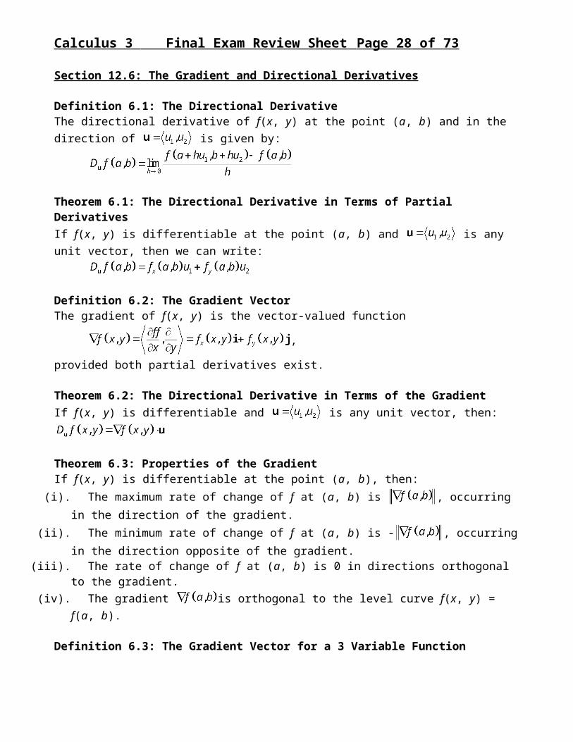
Section 12.6: The Gradient and Directional Derivatives

Definition 6.1: The Directional DerivativeThe directional derivative of f(x, y) at the point (a, b) and in the direction of is given by:

Theorem 6.1: The Directional Derivative in Terms of Partial DerivativesIf f(x, y) is differentiable at the point (a, b) and is any unit vector, then we can write:

Definition 6.2: The Gradient VectorThe gradient of f(x, y) is the vector-valued function

,

provided both partial derivatives exist.

Theorem 6.2: The Directional Derivative in Terms of the GradientIf f(x, y) is differentiable and is any unit vector, then:

Theorem 6.3: Properties of the GradientIf f(x, y) is differentiable at the point (a, b), then:(i). The maximum rate of change of f at (a, b) is , occurring in the direction of the

gradient.(ii). The minimum rate of change of f at (a, b) is - , occurring in the direction opposite of

the gradient.(iii). The rate of change of f at (a, b) is 0 in directions orthogonal to the gradient.(iv). The gradient is orthogonal to the level curve f(x, y) = f(a, b).

Definition 6.3: The Gradient Vector for a 3 Variable FunctionThe directional derivative of f(x, y, z) at the point (a, b, c) and in the direction of is given by:

The gradient of f(x, y, z) is the vector-valued function

.


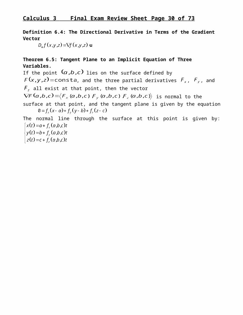
Definition 6.4: The Directional Derivative in Terms of the Gradient Vector

Theorem 6.5: Tangent Plane to an Implicit Equation of Three Variables.If the point lies on the surface defined by , and the three partial derivatives , , and all exist at that point, then the vector

is normal to the surface at that point, and the tangent plane is given by the equation

The normal line through the surface at this point is given by:


Section 12.7: Extrema of Functions of Several Variables

Definition 7.1: Local ExtremaWe call f(a, b) a local maximum of f if there is an open disk R cantered at point (a, b) for which f(a, b) f(x, y) for all (x, y) R. Similarly, we call f(a, b) a local minimum of f if there is an open disk R cantered at point (a, b) for which f(a, b) f(x, y) for all (x, y) R. In either case, f(a, b) is called a local extremum.

Definition 7.2: Critical PointThe point (a, b) is a critical point of the function f(x, y) if (a, b) is in the domain of f and either

or one or both of and do not exist at (a, b).

Theorem 7.1: Condition for a Local ExtremumIf f(x, y) has a local extremum at (a, b), then (a, b) must be a critical point of f.

Definition 7.3: Saddle PointThe point P(a, b, f(a, b)) is a saddle point of z = f(x, y) if (a, b) is a critical point of f and if every open disk centered at (a, b) contains points (x, y) in the domain of f for which f(x, y) < f(a, b) and points (x, y) in the domain of f for which f(x, y) > f(a, b).

Theorem 7.2: Second Derivatives TestSuppose that f(x, y) has continuous second-order partial derivatives in some open disk containing the point (a, b) and that fx(a, b) = fy(a, b) = 0. Define the discriminant D for the point (a, b) by:

D(a, b) = fxx(a, b)fyy(a, b) – [fxy(a, b)]2.(i). If D(a, b) > 0 and fxx(a, b) > 0, then f has a local minimum at (a, b).

(ii). If D(a, b) > 0 and fxx(a, b) < 0, then f has a local maximum at (a, b).(iii). If D(a, b) < 0, then f has a saddle point at (a, b).(iv). If D(a, b) = 0, then no conclusion can be drawn.


One very useful application of max/min theory for functions of two variables is the statistical technique of linear regression, which is a particular case of a more general technique called least squares. Linear regression involves finding a line of “best fit” for a given set of data points. The goal is to find the line that minimizes the sum of the squares of the vertical distances between the data points and the line. This problem can be formulated as a minimization problem involving finding the absolute minimum of a certain function f (the square of the residuals) of the two variables m and b.

You can show that, in general, for n data points (x1, y1), (x2, y2), …, (xn, yn), the linear least square fit yields the two equations

Which have solution


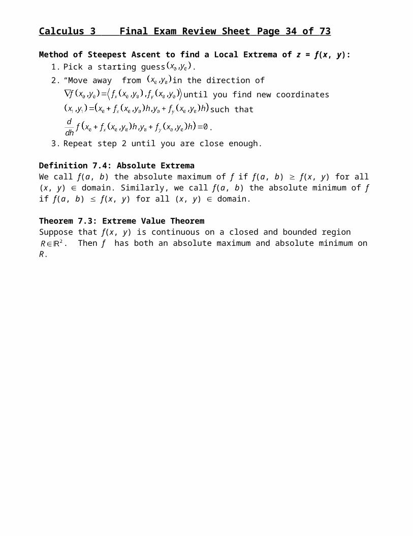
Method of Steepest Ascent to find a Local Extrema of z = f(x, y):1. Pick a starting guess .

2. “Move away” from in the direction of until you

find new coordinates such that

.

3. Repeat step 2 until you are close enough.

Definition 7.4: Absolute ExtremaWe call f(a, b) the absolute maximum of f if f(a, b) f(x, y) for all (x, y) domain. Similarly, we call f(a, b) the absolute minimum of f if f(a, b) f(x, y) for all (x, y) domain.

Theorem 7.3: Extreme Value TheoremSuppose that f(x, y) is continuous on a closed and bounded region . Then f has both an absolute maximum and absolute minimum on R.


Section 12.8: Constrained Optimization and Lagrange Multipliers

Theorem 8.1: If and are functions with continuous first partial derivatives and

on the surface and either the minimum or maximum value of subject to the

constraint occurs at , then

for some constant (called the Lagrange multiplier).

Notice that Theorem 8.1 implies a system of four equations in four variables to be solved:

When Theorem 8.1 is applied to functions of two variables, it implies solving a system of three equations in three unknowns:

Optimization with two constraints:To optimize the function subject to the constraints and , solve

Notice that two constraints on a function of three variables implies a system of five equations in five variables to be solved:


Section 13.1: Double Integrals

Definition 1.1: The Definite Integral of a Function of a Single VariableFor any function f defined on the interval [a, b] and ||P|| (the norm of the partition) defined as the maximum of all the intervals on [a, b] (i.e., ||P|| = max{xi}), the definite integral of f on [a, b] is:

,

provided the limit exists and is the same for all values of the evaluation points ci [xi-1, xi] for i = 1, 2, …, n. In this case, we say f is integrable on [a, b].

Riemann Sum Over a Region:

Definition 1.2: Double Integral of a Function of Two Variables Over a Rectangular RegionFor any function f(x, y) defined on the rectangle R = {(x, y) | a ≤ x ≤ b, c ≤ y ≤ d}, and ||P|| (the norm of the partition) defined as the maximum diagonal of any rectangle in the partition, the double integral of f over R is defined as:

,

provided the limit exists and is the same for all choices of the evaluation points (ui, vi) R for i = 1, 2, …, n. In this case, we say f is integrable over R.

Theorem 1.1: Fubini’s Theorem (Order of Integration is Interchangeable)If a function f(x, y) is integrable on the rectangle R = {(x, y) | a ≤ x ≤ b, c ≤ y ≤ d}, then we can write the double integral of f over R as either of the iterated integrals:

.

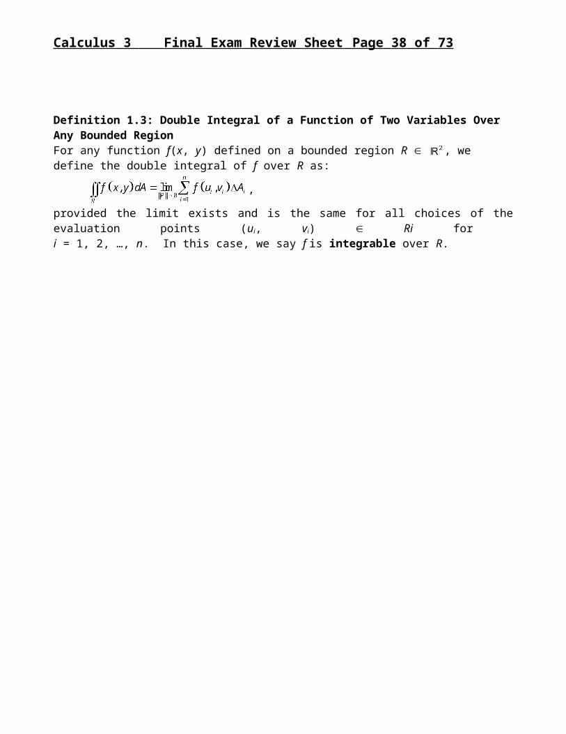
Definition 1.3: Double Integral of a Function of Two Variables Over Any Bounded RegionFor any function f(x, y) defined on a bounded region R , we define the double integral of f over R as:

,

provided the limit exists and is the same for all choices of the evaluation points (ui, vi) Ri for i = 1, 2, …, n. In this case, we say f is integrable over R.


Theorem 1.2: Double Integral Over a Region with Nonconstant Bounds in the x DirectionIf a function f(x, y) is continuous on a bounded region R defined by R = {(x, y) | a ≤ x ≤ b, g1(x) ≤ y ≤ g2(x)} for continuous functions g1 and g2 where g1(x) ≤ g2(x) for all x [a, b], then:

.

Theorem 1.3: Double Integral Over a Region with Nonconstant Bounds in the y DirectionIf a function f(x, y) is continuous on a bounded region R defined by R = {(x, y) | h1(y) ≤ x ≤ h2(y)} c ≤ y ≤ d} for continuous functions h1 and h2 where h1(x) ≤ h2(x) for all y [c, d], then:

.

Theorem 1.4: Linear Combinations of Double IntegralsLet the function f(x, y) and g(x, y) be integrable over the region R R , and let c be any constant. Then the following hold:

i.

ii.

iii. if R = R1 R2, where R1 and R2 are nonoverlapping regions, then

.


Section 13.2: Area, Volume, and Center of MassDouble Riemann Sum Over a Region to Compute Volume under the Surface z = f(x, y):

Note: if we pick the upper surface of z = 1, then

Application of Double Integrals: First Moment and Center of MassGiven a flat plate (or lamina) in the shape of some bounded region R with an area density (x, y), the mass of the lamina is given by:

.

The (first) moments with respect to the x- and y-axes are defined by:

The center of mass of the lamina is given by:

Application of Double Integrals: Second Moment and Moments of Inertia

The (second) moments, or moments of inertia, of a lamina with respect to the x- and y-axes are defined by:


Section 13.3: Double Integrals in Polar CoordinatesBig idea: Making a change of variables to polar coordinates (x = rcos(), y = rsin()) can make many integrals easier to compute. The differential area element in polar coordinates is dA = rdrd.

Cartesian polar conversion formulas:x = rcos() and y = rsin(), which implies x2 + y2 = r2

In addition to making the substitution f(x, y) = f(rcos(), rsin()),we also need to: Describe the region of integration R in terms of r and , which is usually pretty easy to do. Write the differential element of surface area dA in terms of r and , which is just a formula

derived below that you have to remember.

A rr dA = rdrd.

Theorem 3.1: Fubini’s TheoremIf f(r, ) is continuous on the region R = {(r, ) | ≤ ≤ , g1() ≤ r ≤ g2()}, where 0 ≤ g1() ≤ g2() for all [, ], then:

.

Theorem Not-Important-Enough-To-Get-A-Number-Because-No-One-Ever-Uses-It: If f(r, ) is continuous on the region R = {(r, ) | h1(r) ≤ ≤ h2(r)}, a ≤ r ≤ b}, where h1(r) ≤ h2(r) for all r [a, b], then:

.


Section 13.4: Surface Area

Big skill: You should be able to compute the area of a surface defined by a function of two variables

using the formula .

Section 13.5: Triple IntegralsDefinition 5.1: The Definite Integral of a Function of Three VariablesFor any function f(x, y, z) defined in the rectangular box Q = {(x, y, z) | a ≤ x ≤ b, c ≤ y ≤ d, r ≤ z ≤ s }, and ||P|| (the norm of the partition) defined as the maximum diagonal of any rectangular box region in the partition, the triple integral of f over Q is defined as:

,

provided the limit exists and is the same for all choices of the evaluation points (ui, vi, wi) Qi for i = 1, 2, …, n. In this case, we say f is integrable over Q.

Theorem 5.1: Fubini’s Theorem (Order of Integration is Interchangeable)If a function f(x, y) is integrable on the box Q = {(x, y, z) | a ≤ x ≤ b, c ≤ y ≤ d, r ≤ z ≤ s }, then we can write the triple integral of f over Q as:

.

Definition 5.2: Triple Integral of a Function of Three Variables Over Any Bounded VolumeFor any function f(x, y, z) defined on the bounded solid Q, we define the triple integral of f over Q as:

,

provided the limit exists and is the same for all choices of the evaluation points (ui, vi, wi) Qi for i = 1, 2, …, n. In this case, we say f is integrable over Q.


Special Case of a Triple Integral over a Bounded Volume:If Q has the form Q = {(x, y, z) | (x, y) R (a bounded region in the xy plane) and g1(x, y) ≤ z ≤ g2(x, y)}, then

Application of Triple Integrals: First Moment and Center of MassGiven a shape bounding a region Q with a density (x, y, z), the mass of the shape is given by:

.

The first moment with respect to the yz plane is defined by:

The first moment with respect to the xz plane is defined by:

The first moment with respect to the xy plane is defined by:

The center of mass of the shape is given by:


Section 13.6: Cylindrical Coordinates

Special Case of a Triple Integral over a Bounded Volume Using Cylindrical Coordinates:If Q has the form Q = {(r, , z) | (r, ) R and k1(r, ) ≤ z ≤ k2(r, )}, and R has the formR = {(r, ) | ≤ ≤ and g1() ≤ r ≤ g2() },then

Section 13.7: Spherical CoordinatesBig idea: Integrals involving integration volumes and integrands that are spherically symmetric are more easily integrated using spherical coordinates.

Big skill: You should be able to do a triple integral in spherical coordinates.


Triple Integral over a Bounded Volume Using Spherical Coordinates:

Note:

Section 13.8: Change of Variables in Multiple Integrals

Definition 8.1: Jacobian of a TransformationThe determinant

is called the Jacobian of a transformation T and is written using the notation

Theorem 8.1: Change of Variables in Double IntegralsIf a region S in the u-v plane is mapped onto the region R in the x-y plane by the one-to-one transformation T defined by and , where g and h have continuous first

derivatives on S, and if f is continuous on R and the Jacobian is nonzero on S, then

.


Change of variables for triple integrals:In three dimensions, a change of variables is fairly analogous to the two dimensional case:Given a transformation T from a region S of u-v-w space onto a region R of x-y-z space, specified by the functions

, , and , the Jacobian is defined as:

Theorem 8.2: Change of Variables in Triple IntegralsIf a region S in u-v-w space is mapped onto the region R in x-y-z space by the one-to-one transformation T defined by , , and , where g, h, and have

continuous first derivatives on S, and if f is continuous on R and the Jacobian is nonzero on

S, then

.


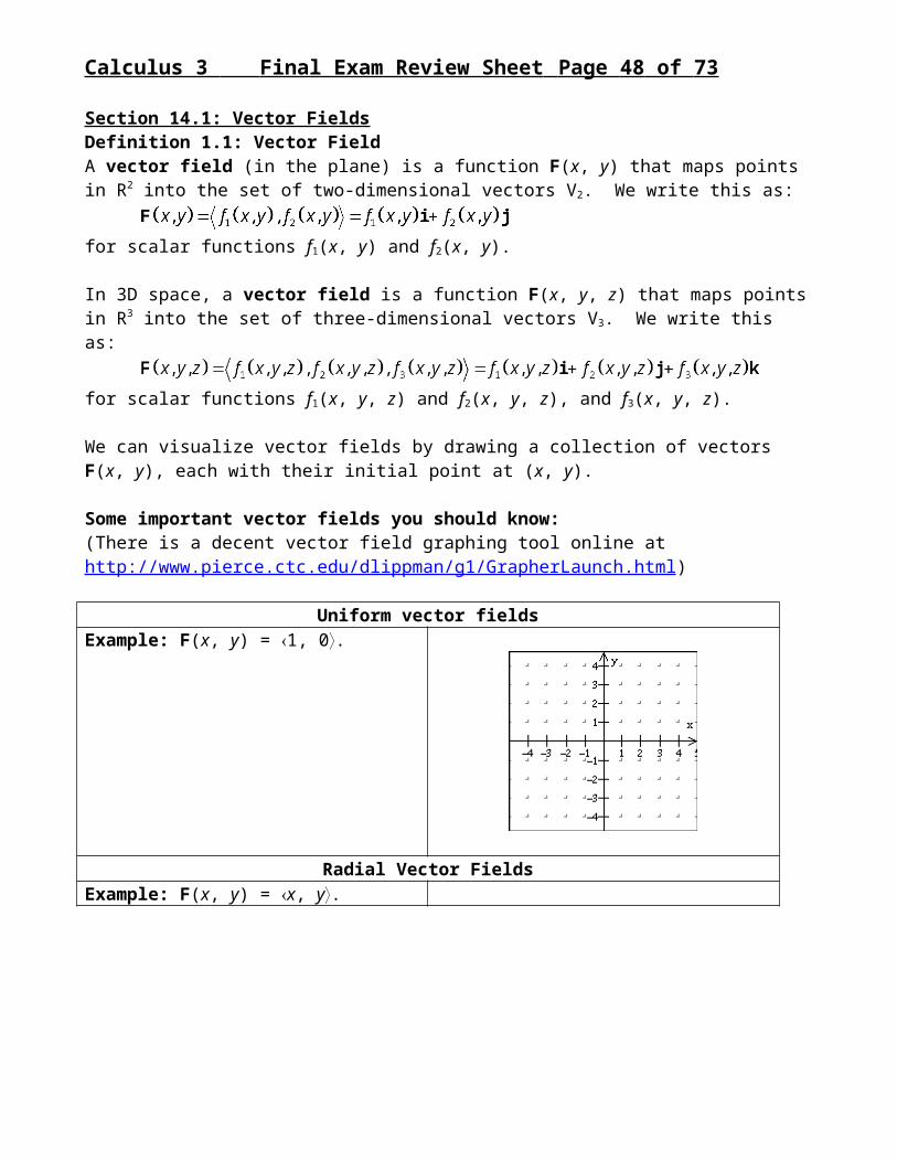
Section 14.1: Vector FieldsDefinition 1.1: Vector FieldA vector field (in the plane) is a function F(x, y) that maps points in R2 into the set of two-dimensional vectors V2. We write this as:

for scalar functions f1(x, y) and f2(x, y).

In 3D space, a vector field is a function F(x, y, z) that maps points in R3 into the set of three-dimensional vectors V3. We write this as:

for scalar functions f1(x, y, z) and f2(x, y, z), and f3(x, y, z).

We can visualize vector fields by drawing a collection of vectors F(x, y), each with their initial point at (x, y).

Some important vector fields you should know:(There is a decent vector field graphing tool online at http://www.pierce.ctc.edu/dlippman/g1/GrapherLaunch.html)

Uniform vector fieldsExample: F(x, y) = 1, 0.

Radial Vector FieldsExample: F(x, y) = x, y.

http://www.pierce.ctc.edu/dlippman/g1/GrapherLaunch.html


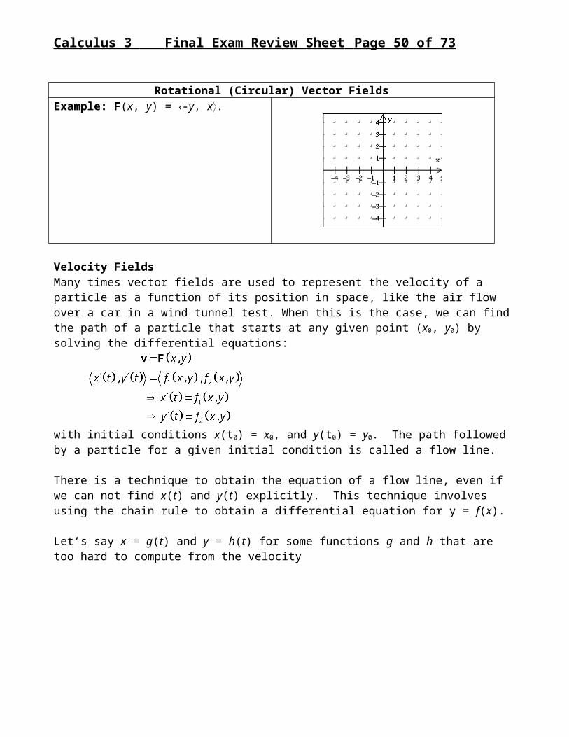
Rotational (Circular) Vector FieldsExample: F(x, y) = -y, x.

Velocity FieldsMany times vector fields are used to represent the velocity of a particle as a function of its position in space, like the air flow over a car in a wind tunnel test. When this is the case, we can find the path of a particle that starts at any given point (x0, y0) by solving the differential equations:

with initial conditions x(t0) = x0, and y(t0) = y0. The path followed by a particle for a given initial condition is called a flow line.

There is a technique to obtain the equation of a flow line, even if we can not find x(t) and y(t) explicitly. This technique involves using the chain rule to obtain a differential equation for y = f(x).

Let’s say x = g(t) and y = h(t) for some functions g and h that are too hard to compute from the velocity

When the right hand side is separable, we know how to solve this differential equation…


Definition 1.2: Gradient Fields and Potential FunctionsThe vector field is called gradient field for any scalar function f(x, y). f is also called the potential function for F. Whenever for some scalar function f, we refer to F as a conservative vector field.

Clearly, given any differentiable scalar function , one can always define a corresponding vector field by computing .

However, the converse of this statement is not true. That is, given a vector field F(x, y), it is not always possible to find a corresponding potential function f(x, y) such that (but sometimes it is…).

To find a potential function, either integrate or , making sure to leave your constant of

integration as a function of the other variable, then take the partial derivative of your answer with respect to the other variable to find the “constant function” of integration.

Section 14.2: Line IntegralsDefinition 2.1: Line Integral with Respect to Arc LengthThe line integral of f(x, y, z) with respect to arc length along the oriented curve C in three-

dimensional space, written as is defined by

,

provided the limit exists and is the same for all choices of evaluation points.

Theorem 2.1: Evaluation Theorem (for Line Integrals)If f(x, y, z) is continuous in a region D containing a curve C, C can be described parametrically by (x(t), y(t), z(t)) for a t b, and x(t), y(t), and z(t) have continuous first derivatives, then

.

Likewise, if f(x, y) is continuous in a region D containing a curve C, C can be described parametrically by (x(t), y(t)) for a t b, and x(t) and y(t) have continuous first derivatives, then

.

A curve C is called smooth if it can be described parametrically by (x(t), y(t), z(t)) for a t b, x(t), y(t), and z(t) have continuous first derivatives, and on the interval [a, b].


For example, the curve C = (t2, t3, t2) is not smooth on the interval [-1, 1] because when t = 0:

x y

z

This means that the line integral

is undefined, but if we break up the curve into two subpieces C = C1 C2 over the intervals [-1,0] and [0, 1], then we can break up the integral into two subpieces as well. A curve that can be subdivided into smooth subpieces is called piecewise smooth.

Theorem 2.2: Line Integrals on a Piecewise Smooth CurveIf f(x, y, z) is continuous in a region D containing an oriented curve C, and C is piecewise-smooth with C = C1 C2 … Cn and all the Ci are smooth and the terminal point of Ci is the initial point of Ci+1 for all i = 1, 2, … n-1, THEN

AND

Geometric interpretation of the line integral:

Just as is the area bounded by x = a, x = b, y = 0 and y = f(x),

is the area of the “vertical” surface bounded by the “vertical” line

through (x(a), y(a)), the vertical line through (x(b), y(b)), the parametric curve (x(t), y(t), 0), and the parametric curve ( x(t), y(t), f(x(t), y(t)) ).

Theorem 2.3: Arc Length of a Curve from a Line Integral


For any piecewise-smooth curve C, gives the arc length of the curve C.

Next, we worry about evaluating a line integral where the integrand is the dot product of a vector field and the differential tangent vector to the curve, as arises in the computation of work:

Definition 2.2: Component-Wise Line IntegralsThe line integral of f(x, y, z) with respect to x along the oriented curve C in three-dimensional space

is written as and is defined by:

,


The line integral of f(x, y, z) with respect to y along the oriented curve C in three-dimensional space


,


The line integral of f(x, y, z) with respect to z along the oriented curve C in three-dimensional space


,


Theorem 2.4: Evaluation Theorem (for Component-Wise Line Integrals)If f(x, y, z) is continuous in a region D containing a curve C, C can be described parametrically by (x(t), y(t), z(t)) for a t b, and x(t), y(t), and z(t) have continuous first derivatives, then

.


Theorem 2.5: Evaluation Theorem (for Component-Wise Line Integrals)If f(x, y, z) is continuous in a region D containing an oriented curve C, then:If C is piecewise-smooth:

If C is piecewise-smooth and forms a closed loop:

Consequence:

Section 14.3: Independence of Path and Conservative Vector Fields

Vocabulary: the line integral is path independent in a domain D if the integral is the same for

every path in D that has the same beginning and ending points.

Definition 3.1: Connected RegionA region (for n 2) is called connected if every pair of points in D can be connected by a piece-wise smooth curve lying entirely in D.


Theorem 3.1: Path Independence of the Line Integral of a Conservative Vector FieldIf the vector field is continuous on the open, connected region ,

then the line integral is independent of path in D if and only if F is conservative in D.

Theorem 3.2: Fundamental Theorem for Line Integrals in Two VariablesIf the vector field is continuous on the open, connected region ,

C is any piecewise-smooth curve lying in D with initial point and terminal point , and

F is conservative in D with , then

.

What happens if the curve C starts and ends at the same point? We call a curve C closed if its endpoints are the same, which can be described mathematically as:

for .

Theorem 3.3: The Line Integral of a Conservative Vector Field along a Closed Curve is ZeroIf the vector field is continuous on the open, connected region , then F is conservative

on D if and only if for every piecewise-smooth curve C lying in D.

Here we can see why the word conservative is used to describe these vector fields: if we think of F as a “force field”, then moving an object through the field along a closed path results in no net work being done, so energy is conserved when the object starts and stops at the same point.

Here is a simple test for whether a vector field is conservative:Theorem 3.4If and have continuous first partial derivatives on a simply-connected region

, then is independent of path in D if and only if

for all (x, y) in D.


Conservative Vector FieldsIf the vector field is continuous on the open, simply-connected

region and and have continuous first partial derivatives on D, then the following five statements are equivalent (i.e., they are either all true or all false)

1. is conservative in D.

2. is a gradient field in D. (i.e., ).

3. is independent of path in D.

4. foe every piecewise-smooth closed curve C lying in D.

5. for all (x, y) in D.

Theorem 3.5: Fundamental Theorem for Line Integrals in Three VariablesIf the vector field is continuous on the open, connected region , then the line

integral is independent of path in D if and only if F is conservative in D. That is,

for all (x, y, z) in D for some scalar function f (the potential function for F).

Further, any for any piecewise-smooth curve C lying in D with initial point and terminal

point , it is true that

.

Another way to tell if a three-component vector field is conservative is to use partial derivatives like we did with two-component fields:


Remember the last row of equalities when we later learn that another condition for a conservative vector field is if its curl is zero:

Section 14.4: Green's Theorem

Vocabulary:Curve C: A curve C is called simple if it does not intersect itself except at the endpoints.

A simple closed curve C has positive orientation if the region R that it bounds “stays to the left” of C as it is traversed.

The notation is used to denote a line integral along a simple closed curve C with a positive

orientation.


Theorem 4.1: Green’s TheoremIf C is a piecewise-smooth, simple closed curve in the plane with positive orientation, R is the region enclosed by C together with C, and are continuous with continuous first partial derivatives in some open region D, and R D, then

.

Vocabulary:

is the contour C that bounds a region R. Thus, .

Theorem 4.2:Suppose and have continuous first partial derivatives on a simply-connected region

D. Then is independent of path if and only if for all

(x, y) in D.

Section 14.5: Curl and Divergence

Definition 5.1: Curl of a Vector FieldThe curl of the vector field is the vector field

,

defined at all points at which the partial derivatives exist.

Alternative notation:


Definition 5.2: Divergence of a Vector FieldThe divergence of the vector field is the scalar function

,

defined at all points at which the partial derivatives exist.

Alternative notation:

Vocabulary: irrotational fluid does not tend to rotate at a given point (curl is zero)source-free / incompressible amount that flows in is equal to amount that flows out (divergence is zero)

Theorem 5.1: A Conservative Field is IrrotationalIf a conservative vector field has components with continuous first-order partial derivatives throughout an open region , then .

Theorem 5.2: An Irrotational Vector Field is ConservativeIf a vector field has components with continuous first-order partial derivatives throughout an open region , then F is conservative if and only if

.

Conservative Vector FieldsIf the vector field has components with continuous first partial derivatives on , then the following five statements are equivalent (i.e., they are either all true or all false)




4. for every piecewise-smooth closed curve C lying in D.

5. .


Alterative Form of Green’s Theorem:

Section 14.6: Surface IntegralsDefinition 6.1: Surface Integral

The surface integral of a function g(x, y, z) over a surface S R3, written as , is defined

by

,

provided the limit exists and is the same for all choices of evaluation points .

Notice that we have to do two things to evaluate this integral: Write g(x, y, z) as a function of two variables, since a double integral involves only two

variables. Write dS, the differential element of surface area on the surface S, in terms of dA, the

differential element of surface area in the x-y plane over which the double integration is performed.

In section 13.4, we found the differential surface element dS for a surface S defined by z = f(x, y) to be .

In this section, the book makes the point that is normal to the plane Ti, and so we can define a normal vector to that small area element . The upshot of this approach is the we can define dS as: , which will be useful for thinking about parametrically defined surfaces. This

expression simplifies to .

Theorem 6.1: Evaluation Theorem for Surface IntegralsIf a surface S is given by z = f(x, y) for (x, y) in the region R R2, and f has continuous first partial derivatives, then


Parametric Representation of SurfacesFor a surface defined parametrically as , define

and .

ru and rv will be in the tangent plane at any point, which means .

Definition 6.2: FluxLet be a continuous vector field defined on an oriented surface S with unit normal vector n.

The surface integral of F over S (or the flux of S over S) is given by

Section 14.7: The Divergence TheoremTheorem 7.1: The Divergence Theorem:If F is a vector field whose components have continuous first partial derivatives over some region

bounded by the closed surface Q with an exterior unit normal vector N, then

Section 14.8: Stokes' Theorem

Theorem 8.1: Stokes’s TheoremIf S is an oriented, piecewise-smooth surface with unit normal vector n, is bounded by the simple closed, piece-wise smooth boundary curve S with positive orientation, and F is a vector field whose components have continuous first partial derivatives over some region containing S, then

.


Theorem 8.2: Irrotational Fields are ConservativeSuppose that F(x, y, z) is a vector field whose components have continuous first partial derivatives

throughout the simply-connected open region D R3. Then, curl F = 0 in D if and only if

for every simple closed curve C contained in the region D.

Theorem 8.3: Conservative Vector FieldsConservative Vector FieldsIf the vector field has components with continuous first partial derivatives in a simply-connected region on D, then the following five statements are equivalent (i.e., they are either all true or all false)




4. for every piecewise-smooth closed curve C lying in D.

5. is irrotational. (i.e., ).


Section 15.1: Second-Order Differential Equations with Constant CoefficientsBig idea: Linear second-order differential equations with constant coefficients can be solved by assuming a solution with an exponential form: i.e., has solution or

for some values r.

Here are four foundational differential equations and their solutions:

Note that the most general solution of the last two is a linear combination of both answers. This is a general result: if you can find two linearly independent solutions of a second-order

equation, then all possible solutions can be written as a linear combination of those two solutions.

The constants in the linear combination are determined by the initial value problem. Cool trick: you can write the trigonometric solution as a single sine or cosine.

o ,

o where

Cool trick: you can write the sum of exponentials as a sum of hyperbolics. Also notice that the trig function and exponential function are related by Euler’s Formula:

o

To solve a second-order differential equation with constant coefficients:,

assume a solution of the form (where r may be a complex number), plug this assumed function into the equation, and find the values of r that satisfy the resulting characteristic equation:


Section 15.2: Non-Homogeneous Equations: Undetermined CoefficientsIn section 15.1, we found that has solution (or ) for some values r. Equations of this form (with zero on the right-hand side) are called homogeneous.

In this section, we extend the equation we can solve to: (for some given

function ). Equations of this form (with a function on the right-hand side) are called nonhomogeneous.

The general solution to the nonhomogeneous equation will be the general solution of the corresponding homogeneous equation plus one or more additional terms that called the particular solution. This is essentially because we can write this linear nonhomogeneous equation as

.

Theorem 2.1: General Solution of a Nonhomogeneous, Linear Second-Order Differential Equation

Let be the general solution of the homogeneous equation

, and let be any solution of the nonhomogeneous equation

. Then the general solution of the nonhomogeneous equation is:

To solve the nonhomogeneous equations in this section, we make use of the “Method of Undetermined Coefficients,” which basically amounts to “make a guess and find the multiplicative constants that make the guess work.”

Steps to solve the nonhomogeneous equation :

Solve the corresponding homogeneous equation . Make a guess for the particular solution:

o If , then guess If are roots of the characteristic equation, then chose

.

o If , then guess

If is a single root of the characteristic equation, then chose .

If is a double root of the characteristic equation, then chose .

o If (i.e., a polynomial of degree n), then guess (i.e., another polynomial of degree n).

If is a single root of the characteristic equation, then chose .


If is a double root of the characteristic equation, then chose .

o If is a product of the above three types of functions, then choose a particular solution that is a product of the above particular solutions.

o Multiplying by t or t2 is done to guarantee that no term in the particular solution is a solution of the corresponding homogeneous equation.

Plug in the guess for the particular solution; equate like terms to determine the value(s) of the undetermined coefficient(s).

Write the general solution as the sum of the homogeneous solution and the particular solution.

Section 15.4: Power Series Solutions of Differential Equations

When the coefficients of a second-order differential equation are not constants, but instead are polynomial functions of the independent variable, like , then one way to solve the equation is using a power series technique:

Assume a power series form of the solution

Plug the power series into the equation and equate like terms Obtain a recurrence relation for the coefficients of higher-order terms in terms of the first two

coefficients, then try to obtain an explicit function for the coefficients based on the term index. Write the final answer in terms of those coefficients.

Documents

Calculus 3 Final Exam Review, Spring 2009faculty.madisoncollege.edu/kmirus/20082009C/804233/... · Web viewThus, there is an equivalent of the vertical line test from two dimensions,