Embed Size (px)
Citation preview

CalculusCalculus for Bioinformatics

Aims of the course i
Providing background in calculus to deal with requirements in othermathematical, computational or modelling issues to appear further.
Providing calculus tools and strategies to endow the student with aminimal experience to study biological phenomena in a formal andcooperative way.

Competencies iiGeneral, basic, specific
Acquire an intra- and interdisciplinary training in both computational and scientificsubjects with a solid basic training in biology.
To acquire knowledge and understanding in a field of study that starts from the basis ofgeneral secondary education, and is typically at a level that although it is supported byadvanced textbooks, includes some aspects that involve knowledge of the forefront of theirfield of study.
To know how to apply the acquired knowledge to the work or vocation in a professionalmanner and have competencies typically demonstrated through devising and defendingarguments and solving problems within their field of study.
To be able to convey information, ideas, problems and solutions to both specialist andnon-specialist audiences.
Develop the skills needed to undertake further studies with a high degree of autonomy.
To manage and exploit all kinds of biological and biomedical information to transform it into knowledge.
To apply mathematical foundations, algorithmic principles and computational theories in the modeling anddesign of biological systems.
To identify meaningful and reliable sources of scientific information to substantiate the state of arts of abioinformatic problem and to address its resolution.

Contents iii
We distinguish 3 types of sessions: theory, seminars and lab.
Theory sessions will be basically devoted to the so-called conceptualline.
Seminar and Lab sessions will be basically devoted to the so-calledpractical line. In both type of sessions, the students will developproposed problems.
In the lab sessions, we will focus mostly on projects requiring the use ofcomputer tools.

Contents ivConceptual line
Conceptual line: It will consist of introductory lectures, motivated by specificbiological problems. The contents of the course will be:
Interpolation and approximation.
Continuity and differentiability.
Integration.
Differential equations and dynamical systems.
Numerical methods.
Every subject will include both expository sessions by the teaching staff andproblem solving sessions.

Contents vPractical line
Practical line: It will turn around short projects where the previousmotivational biological problems will be extended. As the course evolves, theprojects will integrate concepts and techniques from different chapters.
Instances of topics for these problems, which will be described using modelsas simple as possible, are:
Population dynamics.
Models in epidemiology.
Models of neuron activity.

Attention hours vi
Attention hours will hold after every session by appointment.
Toni Guillamon: [email protected]
Àlex Haro: [email protected]

Methodology viiSoftware
The use of the software Octave (or Matlab) will be essential both in Seminarand Lab sessions.
Octave (https://www.gnu.org/software/octave/, distributed under the terms ofthe GNU General Public License).
The support material (slides, problem/project lists, scientific papers,. . . ) willbe posted and updated during the course at the aula@-ESCI.

Bibliography viiiBasic bibliography
Ledder, Glenn. Mathematics for the Life-Sciences: Calculus, Modeling,Probability and Dynamical Systems, Springer Undergraduate Texts inMathematics and Technology, New York : Springer, 2013. ISBN:978-1-461-47276-6.
Strang, Gilbert. Calculus, 2nd edition, Wellesley-Cambridge Press, 2010. ISBN978-09802327-4-5. Also available at the MIT Open CourseWare.http://ocw.mit.edu/resources/res-18-001-calculus-online-textbook-spring-2005/textbook/
Allman, Elizabeth S.; Rhodes, John A. Mathematical models in biology: an introduction.Cambridge: Cambridge University Press, 2004. ISBN 978-0-521-81980-0. Seehttp://cataleg.upc.edu/record=b1297072 S1*cat
Istas, Jacques. Mathematical modeling for the life sciences [on line]. Berlin: Springer, 2005.
Available on: http://dx.doi.org/10.1007/3-540-27877-X. ISBN 354025305X.

Bibliography ixSupplementary bibliography
Salas, Saturnino L.; Etgen, Garret T.; Hille, Einar. Calculus: One and Several Variables, 10thEdition. Wiley [hardcover: January 2007, ISBN : 978-0-471-69804-3] [electronic version:August 2010, ISBN: 978-0-470-47276-7]
Ermentrout, Bard G.; Terman, David H. Mathematical foundations of neuroscience. New York:Springer, 2010. ISBN 978-0-387-87708-2.
Hirsch, Morris W.; Smale, Stephen. Differential equations, dynamical systems, and linearalgebra. Academic Press; American Elsevier Publishing Co., 1975. ISBN :978-0-720-42609-0.
Murray, J.D. Mathematical biology [on line]. 3rd ed. Berlin: Springer, 2002. Available on:http://link.springer.com/book/10.1007/b98868 (volume 1). ISBN 978-0-387-95223-9.
Keener, James P.; Sneyd, James. Mathematical physiology. Vol 1. 2nd ed. New York:
Springer Verlag, 2009. ISBN 978-0-387-75846-6.

Assessment x
A1 Assessment of the concepts and seminar projects introduced in Weeks1–4. Week 5 (October 17th). Weight/value: 20%+10%
A2 Assessment of practical abilities in solving short projects. Week 10(November 23rd). Weight/value: 20%
A3 Assessment of concepts and projects introduced along the course.Week 12 (December 12th). Weight/value: 50%
To obtain a PASS it is necessary to have obtained a grade above 3 over 10 inA1, A2 and A3.

Lecture 1 1
Calculus and modeling

Calculus 2What is it?
Calculus (from Latin calculus, literally "small pebble used for counting") is themathematical study of change, in the same way that geometry is the study ofshape and algebra is the study of operations and their application to solvingequations.
Calculus has two major branches:
differential calculus (concerning rates of change and slopes of curves);
integral calculus (concerning accumulation of quantities and the areasbetween curves);
Both branches are related to each other by the fundamental theorem ofcalculus.

Calculus 3Who invented it?
Modern calculus is considered to have been developed from 17th century byIsaac Newton and Gottfried Leibniz.
Isaac Newton (1643-1727) Gottfried W. Leibniz (1646-1716)
The Kerala school in India had already developed some rudiments of calculusat least 200 years before!

Calculus 4... but why?
Calculus is one of the greatest intellectual achievements ofhumankind. It allows us to solve mathematical problems that cannotbe solved with ordinary algebra, and that in turn allows us to makepredictions about the behavior of real-world systems that could notbe made with algebra alone. (Ledder)

Mathematical models 5The scientific method
The sciences do not try to explain, theyhardly even try to interpret, they mainly makemodels. By a model is meant a mathemati-cal construct which, with the addition of cer-tain verbal interpretations, describes obser-ved phenomena. The justification of such amathematical construct is solely and preci-sely that it is expected to work-that is, cor-rectly to describe phenomena from a reaso-nably wide area. (Von Neumann)
John von Neumann(1903-1957)

Mathematical models 6Characteristics
A mathematical model is a description of a system using mathematicalconcepts and language.
A mathematical model is an approximation of a real phenomenon, that has tobe tested by experiment.
The model has a certain scope, a validity domain.
A model may help to explain a system and to study the effects of differentcomponents, and to make predictions about behavior.
Qualitative models: idealized models that let us to describe the main featuresof a phenomenon.
Quantitative models: let us to make predictions, and simulations.

Mathematical models 7An example: the planetary motions (I)
Johannes Kepler (1571-1630), mathematicianand astronomer, discovered that the Earth andthe rest of planets move in elliptic orbits aroundde Sun, postulating the three fundamental lawsof the planetary motions.
Isaac Newton (1643-1727), mathematician,physicist and astronomer, mathematically provedthe three Kepler’s laws from his own laws ofmotion and law of universal gravitation.

Mathematical models 8An example: the planetary motions (II)
U.J. Le Verrier (1811-1877) and J.C. Adams (1819-1892), independently,predicted the existence of an eighth planet perturbing the orbit ofUranus, that was discovered in 1791.
The planet Neptune was discovered by the astronomer J.G. Galle en1845, in the previously computed position.
A cartoon published in France about the controversy over the discovery of Nep-
tune. Adams seeks the planet and finds it in the pages of Le Verrier’s book.

Mathematical models 9An example: the planetary motions (III)
Le Verrier discovered in 1859 a discrepancy in the orbit of Mercury, thatwas not predicted by Newton’s mechanics.
Albert Einstein (1879-1955),physicist-mathematician, improved the theory ofgravitation in 1915, with the Theory of GeneralRelativity, and explained the orbit of Mercury.
Newton’s gravitational theory is nowadays used in most of the spacemissions.
Einstein’s gravitational theory is used in the Global Positioning System (GPS).

Evolutionary processes 10Determinism ...
An evolutionary process, a system that evolves with time, is said to be:
finite-dimensional if the phase space, the set of all possible states of theprocess, can be identified with an (open) set of the n-dimensional space;
deterministic if its evolution is determined by its state at the present time;
differentiable if the evolution depends not only continuously, but alsodifferentiability, with respect to time, the state at the present time andother parameters of the phenomenon.
The identification of phase space with an n-dimensional space lead to thegeometrization of evolutionary processes, since evolutions are identified withgraphs of functions of the state variables with respect to time, known astrajectories.

Evolutionary processes 11... leads to predictivity
The properties of continuity and differentiability are very useful to makepredictions:
since initial data and parameters are only known with finite accuracy,continuity is important to avoid “jumps” in the behavior of the systemwhen slightly perturbing it;
differentiability is useful to estimate rates of changes with respect to time(velocity), initial conditions and parameters;
predictions are produced by integrating the law of evolution of thesystem, which encodes the relations between the velocities and thestates.
Previous properties are local, but when one considers global properties thereis room for:
changes in the qualitatve structure of a given family of evolutionaryprocesses (bifurcation theory);
long-term unpredictability (chaos theory).
These matters are studied by the theory of dynamical systems.
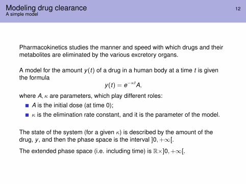
Modeling drug clearance 12A simple model
Pharmacokinetics studies the manner and speed with which drugs and theirmetabolites are eliminated by the various excretory organs.
A model for the amount y(t) of a drug in a human body at a time t is giventhe formula
y(t) = e−κtA,
where A, κ are parameters, which play different roles:
A is the initial dose (at time 0);
κ is the elimination rate constant, and it is the parameter of the model.
The state of the system (for a given κ) is described by the amount of thedrug, y , and then the phase space is the interval ]0,+∞[.
The extended phase space (i.e. including time) is R×]0,+∞[.

Modeling drug clearance 13A particular example
Example1. Jan takes two tablets of acetaminophen (paracetamol) for herheadache, so that the dose is 650 mg. The elimination rate constant isκ = 0.3 h−1.
Question. At what time will there be only 130 mg of acetaminophen in Jan’ssystem?
Solution. Given y = 130 mg, we have to find t so that y = e−κtA. An easycomputation leads to the formula 2
t =1κ
log(
Ay
).
In particular, for the specific problem we are solving, t = 10.3 log 5 ' 5.36 h.
1Example 1.1.1 in Ledder’s2In the following log means natural logarithm, the inverse of the exponential function.
Modeling drug clearance 14Reliability of the results
The fact that the model depends continuously on parameters let us to rely inthe results. Small discrepancies either in parameter or the dose produce justsmall discrepancies in the results.
The elimination rate constant κ can depend not only on the specific drug, butalso on the age, sex, weight and many other instances that depend on theindividual. But the results are qualitatively the same.

Modeling drug clearance 15The half-life for a decaying process
Question. At what time Jan’s system has half of the initial amount ofacetaminophen?
Solution. We are asked to find t 12
so that y(t 12) = 1
2 A. This is very easy fromthe previous formula:
t 12=
log 2κ' 2.31h
Observations:
t 12
is the half-life for the constant decaying system;
t 12
depends on κ, and it does not depend on the initial dose;
Public resources generally provide this quantity for a given drug ratherthan the elimination rate κ, but
κ =1t 1
2
log 2.

Modeling drug clearance 16The law of decay
The rate of change of the amount of drug is the derivative with respect totime:
y(t) = −κe−κtA.
The velocity and the state itself are related by
y(t) = −κy(t).
This is the law of the decay of the drug, a differential equation that encodesall possible evolutions of the system.
Similar laws describe other a priori very different phenomena, such asradioactive decay (useful for 14C dating test) and cooling of bodies.
In general, the differential equation of an evolutionary process is the equationthat relates the rates of change of the states with the states themselves.

Modeling drug clearance 17Solving a simple differential equation
An evolution of the system is (presumably) determined by the initial condition,say y(0) = A.We have then to solve an initial value problem:
y(t) = −κy(t), y(0) = A.
Notice that y(t) > 0, so that we can divide by y(t) to get
−κ =y(t)y(t)
=ddt
(log y(t)).
Integrating from time 0 to t both sides of the equation, we get:
−κt =∫ t
0
ddt
(log y(t)) dt = [log y(t)]t0 = log y(t)− log A = log(
y(t)A
),
where we have used the fundamental theorem of calculus, aka Barrow’s rule.Finally, we get the expected evolution
y(t) = e−κtA.
Modeling drug clearance 18Solving a simple differential equation
Observations:
most of the differential equations can not be solved by hand, and onecan use numerical methods;
global features of the systems can be studied by using qualitative ratherthan quantitative approach.

Modeling drug clearance 19Model test and parameter selection by optimization
Example. Jim has participated in a clinical analysis in order to test the effectsof two tablets of acetaminophen in his body. The results of the analysis areshown in the following table:
Time (h) 0 0.5 1.0 1.5 2.0 2.5 3.0 3.5 4.0
Acetaminophen (mg) 650.0 552.3 471.5 406.7 347.1 297.6 254.9 219.8 184.2
Problem. We want to test the exponential decay behavior y(t) = e−κtA ofthe drug clearance in Jim’s body.
Modeling drug clearance 20Guess and check analysis
0
100
200
300
400
500
600
700
0 0.5 1 1.5 2 2.5 3 3.5 4
Jim datag= 0.30g= 0.31
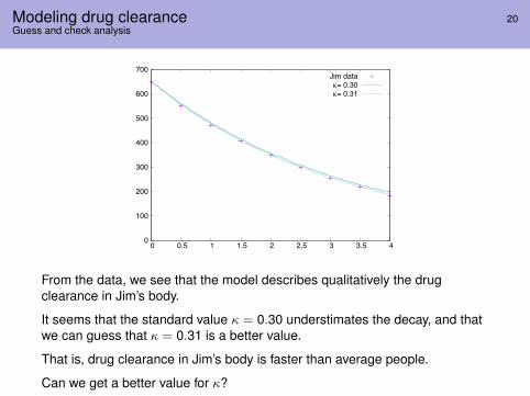
From the data, we see that the model describes qualitatively the drugclearance in Jim’s body.
It seems that the standard value κ = 0.30 understimates the decay, and thatwe can guess that κ = 0.31 is a better value.
That is, drug clearance in Jim’s body is faster than average people.
Can we get a better value for κ?
Modeling drug clearance 21Optimization
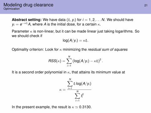
Abstract setting: We have data (ti , yi) for i = 1, 2, . . .N. We should haveyi = e−κti A, where A is the initial dose, for a certain κ.
Parameter κ is non-linear, but it can be made linear just taking logarithms. Sowe should check if
log(A/yi) = κti .
Optimality criterion: Look for κ minimizing the residual sum of squares
RSS(κ) =N∑
i=1
(log(A/yi)− κti)2 .
It is a second order polynomial in κ, that attains its minimum value at
κ =
N∑i=1
ti log(A/yi)
N∑i=1
t2i
In the present example, the result is κ ' 0.3130.

Population dynamics 22Some simple models
Population dynamics is the branch of life sciences that studies the size andage composition of populations as dynamic systems, and the biological andenvironmental processes driving them (such as birth and death rates,migrations, . . . ).
Several simple models for the size x of a biological population:Malthus’ model, or equation of normal reproduction:
x = κx , κ > 0.
The rate of reproduction is proportional (with constant κ) to the numberof organisms present.Velhurst’s model, or logistic equation:
x = ax − bx2, a > 0, b > 0.
The competition of food leads to a decrease of the rate of reproduction,with κ = a− bx .Logistic growth with emigration:
x = ax − bx2 − c, a > 0, b > 0, c > 0.
It includes the effect of the emigration at a constant rate c.
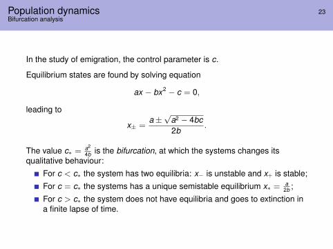
Population dynamics 23Bifurcation analysis
In the study of emigration, the control parameter is c.
Equilibrium states are found by solving equation
ax − bx2 − c = 0,
leading to
x± =a±√
a2 − 4bc2b
.
The value c∗ = a2
4b is the bifurcation, at which the systems changes itsqualitative behaviour:
For c < c∗ the system has two equilibria: x− is unstable and x+ is stable;
For c = c∗ the systems has a unique semistable equilibrium x∗ = a2b ;
For c > c∗ the system does not have equilibria and goes to extinction ina finite lapse of time.

Population dynamics 24Qualitative analysis of harvesting
The previous model can be applied also to the study of harvesting (forinstance, we catch fish of a pond at a constant rate).
We have observed the dramatic changes produced if we harvest too much.
A presumably better way of harvesting is taking a rate proportional to thepopulation. The model is
x = ax − bx2 − px , a > 0, b > 0, p > 0.
This is in fact a logistic model, writen as
x = (a− p)x − bx2.
In order to preserve the population, we take p < a.
The limiting value of the population is x+ = a−pb .
Observation: Bifurcation analysis let us to study the different possiblebehaviours of a system with respect to certain control parameters, so we cantune them appropriately to get a desired effect.

Lecture 2 1
Continuity

Continuity
Definition (the concept of limit).
Examples: elementary functions.
Properties: sum, product, composition.
Resources: Geogebra calculus applets at
http://webspace.ship.edu/msrenault/GeoGebraCalculus/GeoGebraCalculusApplets.html, by Marc
Renault.

Example: match the elementary function
(a) x6 − 3 x5 + 1, (b) 1/(x − 1), (c) ln(x2),(d) exp(x/10) sin(x), (e) 1/(1 + exp(−x)), (f) − x7 + 2.
-5 5 10 15 20 25
-10
-5
5
(A)
-10 -5 5 10
0.2
0.4
0.6
0.8
1(B)
-2 -1 1 2
-20
-15
-10
-5
(C)
-1 1 2 3
-2000
-1500
-1000
-500
500
1000
1500 (D)
-2 -1 1 2 3
-50
50
100
150
200(E)
-3 -2 -1 1 2 3
-2000
-1000
1000
2000(F)

4
Derivatives of one-variable realfunctions

Atmospheric carbon dioxide concentration
Mean annual atmospheric carbon dioxide concentration at MaunaLoa observatory in Hawaii:
Year 1960 1965 1970 1975 1980 1985 1990Average CO2 316.91 320.04 325.68 331.08 338.68 345.87 354.16
Year 1995 2000 2005 2007 2008 2009 2010AverageCO2 360.63 369.40 379.78 383.72 385.57 387.36 389.78
Source: [Ledder]

Atmospheric carbon dioxide concentration
Mean annual atmospheric carbon dioxide concentration at MaunaLoa observatory in Hawaii:
Year 1960 1965 1970 1975 1980 1985 1990Average CO2 316.91 320.04 325.68 331.08 338.68 345.87 354.16
Year 1995 2000 2005 2007 2008 2009 2010AverageCO2 360.63 369.40 379.78 383.72 385.57 387.36 389.78
Average rate period 1960–1970:
∆y∆t
=325.68− 316.91
1970− 1960≈ 0.877
Average rate period 2005–2010:
∆y∆t
=389.78− 379.78
2010− 2005≈ 2.000

Atmospheric carbon dioxide concentration
Year 1960 1965 1970 1975 1980 1985 1990Average CO2 316.91 320.04 325.68 331.08 338.68 345.87 354.16
Year 1995 2000 2005 2007 2008 2009 2010AverageCO2 360.63 369.40 379.78 383.72 385.57 387.36 389.78
Source: www.esrl.noaa.gov/gmd/ccgg/trends/

Atmospheric carbon dioxide concentration
Mean annual atmospheric carbon dioxide concentration at MaunaLoa observatory in Hawaii:
Source: www.esrl.noaa.gov/gmd/ccgg/trends/
In many biological processes, either observed quantities or timeunits are continuous. Even though the number of molecules maybe discrete, the chemical masses, biomasses,. . . can beassumed continuous.We must find a way to understand the rate of change ofcontinuous quantities over continuous time.
Difference quotients
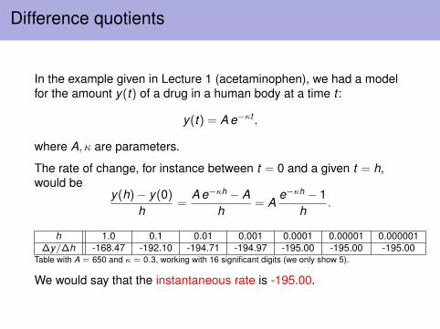
In the example given in Lecture 1 (acetaminophen), we had a modelfor the amount y(t) of a drug in a human body at a time t :
y(t) = A e−κt ,
where A, κ are parameters.
The rate of change, for instance between t = 0 and a given t = h,would be
y(h)− y(0)
h=
A e−κh − Ah
= Ae−κh − 1
h.
h 1.0 0.1 0.01 0.001 0.0001 0.00001 0.000001∆y/∆h -168.47 -192.10 -194.71 -194.97 -195.00 -195.00 -195.00
Table with A = 650 and κ = 0.3, working with 16 significant digits (we only show 5).
We would say that the instantaneous rate is -195.00.
Difference quotients
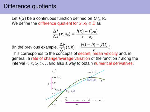
Let f (x) be a continuous function defined on D ⊆ R.We define the difference quotient for x , x0 ∈ D as
∆f∆x
(x , x0) =f (x)− f (x0)
x − x0
(In the previous example,∆y∆t
(t ,h) =y(t + h)− y(t)
h.)
This corresponds to the concepts of secant, mean velocity and, ingeneral, a rate of change/average variation of the function f along theinterval < x , x0 >. . . and also a way to obtain numerical derivatives.

Derivatives
We define the derivative of f at x0 ∈ D as
f ′(x0) :=df (x)
dx(x0) := lim
x→x0
f (x)− f (x0)
x − x0.
(In the previous example, y ′(t) =dydt
(t) = limh→0
y(t + h)− y(t)h
.)
It corresponds to the concepts of tangent, instantaneous velocity and,in general, the instantaneous variation of the function f at the point x0.Note that it involves the concept of limit.

The derivative as a function
When the limit f ′(x) exists for all x ∈ D ⊆ R (D open), we say that f isdifferentiable on D. We can, then, consider f ′ as a new functiondefined on D:
Which curve is f ′(x)? And −f ′′(x)?

The derivative as a function
When the limit f ′(x) exists for all x ∈ D ⊆ R (D open), we say that f isdifferentiable on D. We can, then, consider f ′ as a new functiondefined on D:

Derivatives in biology
We will find derivatives in many problems, mainly:Optimization problems in one and more variables.Differential equations (from the previous lecture):
Law of decay of a drug quantity: y(t) = −κy(t).Malthus-Verhulst-logistic with emigration laws in populationdynamics:
x = ax − bx2 − c, a > 0, b > 0, c > 0.

Computing derivatives
Elementary derivative formulas.General derivative rules.
Remark: Using elementary derivative formulas and general derivativerules we can differentiate any function given explicitly.
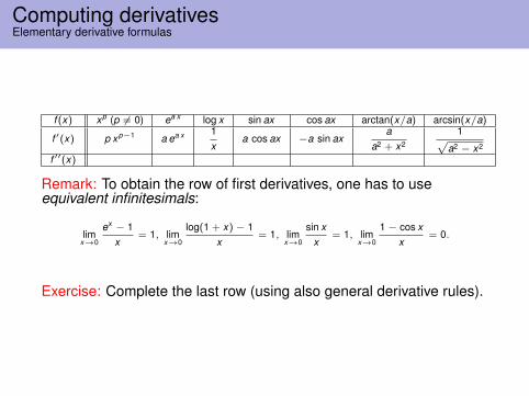
Computing derivativesElementary derivative formulas
f (x) xp (p 6= 0) ea x log x sin ax cos ax arctan(x/a) arcsin(x/a)
f ′(x) p xp−1 a ea x 1x
a cos ax −a sin axa
a2 + x2
1√a2 − x2
f ′′(x)
Remark: To obtain the row of first derivatives, one has to useequivalent infinitesimals:
limx→0
ex − 1x
= 1, limx→0
log(1 + x)− 1x
= 1, limx→0
sin xx
= 1, limx→0
1− cos xx
= 0.
Exercise: Complete the last row (using also general derivative rules).
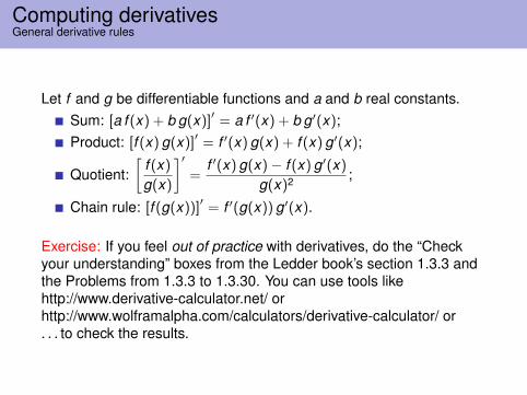
Computing derivativesGeneral derivative rules
Let f and g be differentiable functions and a and b real constants.Sum: [a f (x) + b g(x)]′ = a f ′(x) + b g′(x);Product: [f (x) g(x)]′ = f ′(x) g(x) + f (x) g′(x);
Quotient:[
f (x)
g(x)
]′=
f ′(x) g(x)− f (x) g′(x)
g(x)2 ;
Chain rule: [f (g(x))]′ = f ′(g(x)) g′(x).
Exercise: If you feel out of practice with derivatives, do the “Checkyour understanding” boxes from the Ledder book’s section 1.3.3 andthe Problems from 1.3.3 to 1.3.30. You can use tools likehttp://www.derivative-calculator.net/ orhttp://www.wolframalpha.com/calculators/derivative-calculator/ or. . . to check the results.

The chain rule: interpretation I
The chain rule is an essential technique in mathematical modeling.
Example:t time;x position of any point along the rod (measured from hot end).s(t) location of insect on the x axis;T (x) temperature at any point on the rod;u(t) temperature at insect’s location.
Clearly, u(t) = T (s(t)); we want to know du/dt at some instant t1,assuming that we know s(t) and T (x) for any time (and so, theirderivatives).Let x1 = s(t1). Insects’s position changes as ∆x in a small amount oftime; using linear approximation (see below):
∆x ≈ dsdt
(t1) ∆t .
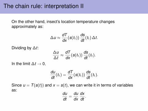
The chain rule: interpretation II
On the other hand, insect’s location temperature changesapproximately as:
∆u ≈ dTdx
(s(t1))dsdt
(t1) ∆t .
Dividing by ∆t :∆u∆t≈ dT
dx(s(t1))
dsdt
(t1).
In the limit ∆t → 0,
dudt
(t1) =dTdx
(s(t1))dsdt
(t1).
Since u = T (s(t)) and x = s(t), we can write it in terms of variablesas:
dudt
=dudx
dxdt.

Tangent line
Since we seek for a straight line passing through (x0, f (x0)) and theslope must be f ′(x0), then the tangent line to a graph y = f (x) at apoint (x0, f (x0)) is given by
y = f (x0) + f ′(x0)(x − x0).
Tangent line to the graph of x3 − 3 x at x = −1.2.

Tangent line
Since we seek for a straight line passing through (x0, f (x0)) and theslope must be f ′(x0), then the tangent line to a graph y = f (x) at apoint (x0, f (x0)) is given by
y = f (x0) + f ′(x0)(x − x0).
Tangent line to the graph of x3 − 3 x at x = −1.2. Zoom 1.

Tangent line
Since we seek for a straight line passing through (x0, f (x0)) and theslope must be f ′(x0), then the tangent line to a graph y = f (x) at apoint (x0, f (x0)) is given by
y = f (x0) + f ′(x0)(x − x0).
Tangent line to the graph of x3 − 3 x at x = −1.2. Zoom 2.

Linear approximation
Tangent line to the graph of x3 − 3 x at x = −1.2. Zoom 2.
y = f (x0) + f ′(x0)(x − x0) ≈ f (x)
Close to x0, taking ∆x = x − x0 and ∆f = f (x)− f (x0), we have that
∆f ≈ f ′(x0) ∆x Linear Approximation

Function growth and extrema
If f ′(x0) = 0, then the tangent line is
y = f (x0) + 0 (x − x0) ≡ f (x0).
A local extremum of a continuous function f is a point x0 where f ′
changes sign.A critical point of a continuous function f is a point x0 wheref ′(x0) = or f ′(x0) does not exist.If f is differentiable, f ′(x0) = 0 is a necessary condition for x0 tobe a local extremum, but not sufficient.The local behavior of a function f near a point x0 is determinedby the lowest order derivative whose value is not zero, providedsuch a nonzero derivative exists.Remark: If f is differentiable, f ′(x0) = 0 and f ′′(x0) > 0, then x0 isa local minimum; if f is differentiable, f ′(x0) = 0 and f ′′(x0) < 0,then x0 is a local maximum.

Function growth and extrema
Example:f (x) = x3 − 2 x2 + b x .
Octave scriptx =-2:0.01:3;
iMax=5
bIni=-2
bFin=4
for i=0:iMax
b=bIni+i*(bFin-bIni)/iMax;
c=i/iMax;
plot(x,x.ˆ3-2*x.ˆ2+b*x,“Color",[c*c,1-c,c*(1-c)],“linewidth",2);
hold on
end
hold off
From b=-2 to b=420
10
0
-10
-20
-303210-1-2
30

Global extrema
Suppose x∗ yields the largest or smallest value of a continuousfunction f (x) on an interval a ≤ x ≤ b. Then either x∗ is a criticalpoint, x∗ = a or x∗ = b.

Example: Fitness of gene pool
The gene responsible for sickle cell disease has two possible alleles, A and a. Individuals with the
aa genotype have sickle cell anemia. Under natural conditions, people with sickle cell anemia did
not live long enough to have children. Since the gene reduces fitness (adaptability), one would
expect it to have been eliminated by natural selection. Indeed, people whose ancestors come from
cold climates do not have the a allele, but this allele is not uncommon in parts of Africa. Individuals
with the Aa genotype have a higher natural resistance to malaria than individuals with the AA
genotype; where malaria is endemic, individuals with the Aa genotype have a longer life
expectancy, which means they are likely to have more surviving children. Thus, the a allele has an
indirect benefit along with its direct liability. To model the population dynamics of the sickle cell
gene, let p be the fraction of A genes in the gene pool. We assume that the fitness of the aa
genotype is 0, the fitness of the Aa genotype is 1, and the fitness of the AA genotype is a parameter
w. According to the theory of genetics, the overall fitness of the gene pool is...
F (p) = w p2 + 2 p (1− p) = · · · = 2 p + (w − 2) p2.

Example: Fitness of gene pool
F (p) = w p2 + 2 p (1− p) = · · · = 2 p + (w − 2) p2.
F (0) = 0; F (1) = w ; p∗ = 1/(2− w) critical point.F (p∗) = p∗ = 1/(2− w).
(Left) Graph for different w . (Right) Critical point in terms of w .
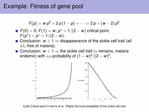
Example: Fitness of gene pool
F (p) = w p2 + 2 p (1− p) = · · · = 2 p + (w − 2) p2.
F (0) = 0; F (1) = w ; p∗ = 1/(2− w) critical point.F (p∗) = p∗ = 1/(2− w).Conclusion: w ≥ 1⇒ disappearance of the sickle cell trait (allAA, free of malaria).Conclusion: w < 1⇒ the sickle cell trait (a remains, malariaendemic) with aa-probability of (1− w)2/(2− w)2.
(Left) Critical point in terms of w . (Right) Survival probability of the sickle cell trait.

Application: The marginal value theorem
Imagine a process occurring at different patches (in general,locations) and consisting of collecting something with increasingdifficulty.
Apples from different trees Distributed parallel computing Animals foraging at different food sources
Trade-off:It costs some time to move from one tree to the next, whichsuggests that you should stay longer at the first tree.However, the apples get harder to pick as time goes on, whichsuggests that you should move to a new tree sooner.
Goal:Find the right amount of perseverance (evolutionary advantages).
Application: The marginal value theorem
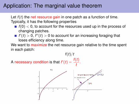
Let f (t) the net resource gain in one patch as a function of time.Typically, it has the following properties
f (0) < 0, to account for the resources used up in the process ofchanging patches.f ′(t) > 0, f ′′(t) > 0 to account for an increasing foraging thatloses efficiency along time.
We want to maximize the net resource gain relative to the time spentin each patch:
f (t)/t
A necessary condition is that f ′(t) =f (t)
t.
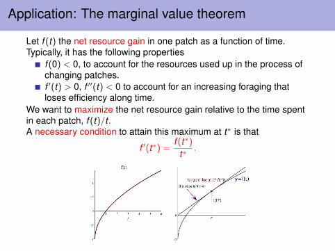
Application: The marginal value theorem
Let f (t) the net resource gain in one patch as a function of time.Typically, it has the following properties
f (0) < 0, to account for the resources used up in the process ofchanging patches.f ′(t) > 0, f ′′(t) < 0 to account for an increasing foraging thatloses efficiency along time.
We want to maximize the net resource gain relative to the time spentin each patch, f (t)/t .A necessary condition to attain this maximum at t∗ is that
f ′(t∗) =f (t∗)
t∗.

Application: The marginal value theorem
Let f (t) the net resource gain in one patch as a function of time withf (0) < 0, f ′(t) > 0, f ′′(t) < 0 to account for the resources usedup in the process of changing patches and an increasingforaging that loses efficiency along time.
A necessary condition (indeed, also sufficient1) for f (t)/t to attain this
maximum at t∗ is that f ′(t∗) =f (t∗)
t∗.
1Prove that (f (t∗)/t∗)′′ = f ′′(t∗)/t3
Lecture 3 1
Numerical solution of equations

An example: the chemical equilibrium 2
Problem:An equimolecular mix of carbon monoxide and oxigen reaches the equilibriumat temperature T = 300◦K and pressure P = 5 atm. The theoretical chemicalreaction is CO + 1
2 O2 CO2, while the real chemical reactions isCO + O2 → xCO + 1
2 (1 + x)O2 + (1− x)CO2, where x is the fraction ofremaining CO. The equation for equilibrium that determines de fraction x is:
Kp =(1− x)(3 + x)1/2
x(x + 1)1/2P1/2 , 0 < x < 1 ,
where Kp = 3.06 is the equilibrium constant for such temperature andpressure.
Question: Which is the value of x?
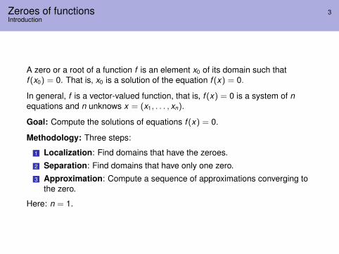
Zeroes of functions 3Introduction
A zero or a root of a function f is an element x0 of its domain such thatf (x0) = 0. That is, x0 is a solution of the equation f (x) = 0.
In general, f is a vector-valued function, that is, f (x) = 0 is a system of nequations and n unknows x = (x1, . . . , xn).
Goal: Compute the solutions of equations f (x) = 0.
Methodology: Three steps:
1 Localization: Find domains that have the zeroes.
2 Separation: Find domains that have only one zero.
3 Approximation: Compute a sequence of approximations converging tothe zero.
Here: n = 1.
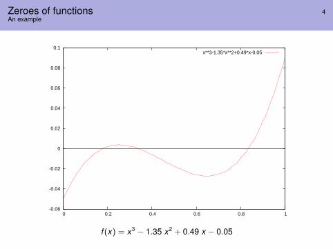
Zeroes of functions 4An example
-0.06
-0.04
-0.02
0
0.02
0.04
0.06
0.08
0.1
0 0.2 0.4 0.6 0.8 1
x**3-1.35*x**2+0.49*x-0.05
f (x) = x3 − 1.35 x2 + 0.49 x − 0.05
Localizing zeroes: Bolzano’s theorem 5Bisection method
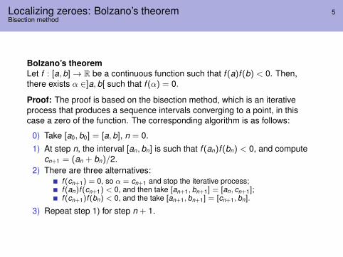
Bolzano’s theoremLet f : [a, b]→ R be a continuous function such that f (a)f (b) < 0. Then,there exists α ∈]a, b[ such that f (α) = 0.
Proof: The proof is based on the bisection method, which is an iterativeprocess that produces a sequence intervals converging to a point, in thiscase a zero of the function. The corresponding algorithm is as follows:
0) Take [a0, b0] = [a, b], n = 0.
1) At step n, the interval [an, bn] is such that f (an)f (bn) < 0, and computecn+1 = (an + bn)/2.
2) There are three alternatives:f (cn+1) = 0, so α = cn+1 and stop the iterative process;f (an)f (cn+1) < 0, and then take [an+1, bn+1] = [an, cn+1];f (cn+1)f (bn) < 0, and the take [an+1, bn+1] = [cn+1, bn].
3) Repeat step 1) for step n + 1.

Localizing zeroes: Bolzano’s theorem 6Bisection method
If the iteration stops is due to the fact we have found α.
Otherwise, we construct a squence of nested intervals
[a, b] = [a0, b0] ⊃ [a1, b1] ⊃ . . . ⊃ [an, bn] ⊃ . . . ,
whose lengths go to 0.
Since the sequence (an)n is increasing, and bounded from above, it has alimit, say α. Analogously, since the sequence (bn)n is decreasing, andbounded from below, then it has also a limit, β.
Since0 = lim
n→∞(bn − an) = β − α,
then β = α.
At this point we use the continuity property of the function f , so that
limn→∞
f (an) = limn→∞
f (bn) = f (α).
Since f (an)f (bn) < 0 for all n, then,
0 ≥ limn→∞
f (an)f (bn) = f (α)2.
But this is only possible if f (α) = 0. �
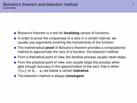
Bolzano’s theorem and bisection method 7Comments
Bolzano’s theorem is a tool for localizing zeroes of functions.
In order to prove the uniqueness of a zero in a certain interval, weusually use arguments involving the monotonicity of the function.
The mathematical proof of Bolzano’s theorem provides a computationalmethod to approximate the zero of a function: the bisection method.
From a theoretical point of view, the iterative process usually never stops.
From the practical point of view, one usually stops the process whengets enough accuracy in the approximation of the zero, that is when|f (cn)| or bn − an are below a certian tolerance.
The bisection method is always convergent.

Example: the equation exp(x − 0.5)− 2x + 0.35 = 0 8Localization of zeroes
Exemple: We want to solve equation f (x) = exp(x − 0.5)− 2x + 0.35.
1) Study of the function.Since f ′(x) = exp(x − 0.5)− 2, then function f has an unique localextremum at xm = log(2) + .5 ' 1.19315. In fact:
f is stricly decreasing at ]−∞, xm[;
f is stricly increasing at ]xm,+∞[;
xm is a global minimum, with f (xm) = 1.35− 2 log(2) ' −0.0362944 < 0.
Moreover, since limx→−∞
f (x) = +∞ and limx→+∞
f (x) = +∞, llavors
f has one zero α1 at ]−∞, xm[;
f has one zero α2 at ]xm,+∞[;
α1 and α2 are the zeroes of f .

Example: the equation exp(x − 0.5)− 2x + 0.35 = 0 9Graphical representation

Example: the equation exp(x − 0.5)− 2x + 0.35 = 0 10Application of bisection method
2) Computation of α1 (with 8 figures): α1 = 0.99639033n an bn bn − an f (an) f (bn) cn+1 f (ci+1)
0 0.950000000 1.050000000 1.0e-01 1.8e-02 -1.7e-02 1.000000000 -1.3e-031 0.950000000 1.000000000 5.0e-02 1.8e-02 -1.3e-03 0.975000000 8.0e-032 0.975000000 1.000000000 2.5e-02 8.0e-03 -1.3e-03 0.987500000 3.2e-033 0.987500000 1.000000000 1.2e-02 3.2e-03 -1.3e-03 0.993750000 9.5e-044 0.993750000 1.000000000 6.2e-03 9.5e-04 -1.3e-03 0.996875000 -1.7e-045 0.993750000 0.996875000 3.1e-03 9.5e-04 -1.7e-04 0.995312500 3.9e-046 0.995312500 0.996875000 1.6e-03 3.9e-04 -1.7e-04 0.996093750 1.1e-047 0.996093750 0.996875000 7.8e-04 1.1e-04 -1.7e-04 0.996484375 -3.4e-058 0.996093750 0.996484375 3.9e-04 1.1e-04 -3.4e-05 0.996289063 3.6e-059 0.996289063 0.996484375 2.0e-04 3.6e-05 -3.4e-05 0.996386719 1.3e-06
10 0.996386719 0.996484375 9.8e-05 1.3e-06 -3.4e-05 0.996435547 -1.6e-0511 0.996386719 0.996435547 4.9e-05 1.3e-06 -1.6e-05 0.996411133 -7.4e-0612 0.996386719 0.996411133 2.4e-05 1.3e-06 -7.4e-06 0.996398926 -3.1e-0613 0.996386719 0.996398926 1.2e-05 1.3e-06 -3.1e-06 0.996392822 -8.9e-0714 0.996386719 0.996392822 6.1e-06 1.3e-06 -8.9e-07 0.996389771 2.0e-0715 0.996389771 0.996392822 3.1e-06 2.0e-07 -8.9e-07 0.996391296 -3.5e-0716 0.996389771 0.996391296 1.5e-06 2.0e-07 -3.5e-07 0.996390533 -7.3e-0817 0.996389771 0.996390533 7.6e-07 2.0e-07 -7.3e-08 0.996390152 6.3e-0818 0.996390152 0.996390533 3.8e-07 6.3e-08 -7.3e-08 0.996390343 -5.3e-0919 0.996390152 0.996390343 1.9e-07 6.3e-08 -5.3e-09 0.996390247 2.9e-0820 0.996390247 0.996390343 9.5e-08 2.9e-08 -5.3e-09 0.996390295 1.2e-0821 0.996390295 0.996390343 4.8e-08 1.2e-08 -5.3e-09 0.996390319 3.2e-0922 0.996390319 0.996390343 2.4e-08 3.2e-09 -5.3e-09 0.996390331 -1.0e-0923 0.996390319 0.996390331 1.2e-08 3.2e-09 -1.0e-09 0.996390325 1.1e-0924 0.996390325 0.996390331 6.0e-09 1.1e-09 -1.0e-09 0.996390328 1.1e-09

Newton’s method 11Description of the method
Problem: Let x0 be an approximate zero of f . How could we improve theestimate?(Assume we know f ′).
Let h be the correction of x0, so that the new approximation is x1 = x0 + h.Then, we would like
0 = f (x0 + h) ≈ f (x0) + f ′(x0)h.
Then, we choose
h = − f (x0)
f ′(x0)
Newton’s method (aka known Newton–Raphson method) consists in, givenan initial approximation x0 of a root of f , generate the sequence ofapproximations (xn)n, by the recurrence:
xn+1 = xn −f (xn)
f ′(xn), n = 0, 1 . . . .

Newton’s method 12Geometrical idea
Newton’s method 13Comments
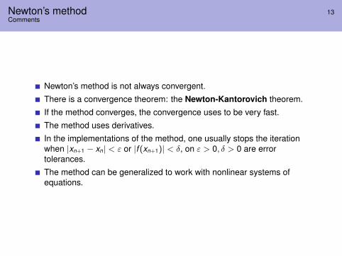
Newton’s method is not always convergent.
There is a convergence theorem: the Newton-Kantorovich theorem.
If the method converges, the convergence uses to be very fast.
The method uses derivatives.
In the implementations of the method, one usually stops the iterationwhen |xn+1 − xn| < ε or |f (xn+1)| < δ, on ε > 0, δ > 0 are errortolerances.
The method can be generalized to work with nonlinear systems ofequations.

Example: the equation exp(x − 0.5)− 2x + 0.35 = 0 14Application of Newton’s method
We compute α1, zero of f (x) = exp(x − 0.5)− 2x + 0.35 at [0.95, 1.05], withNewton’s method, from initial value x0 = 0.95.
n xn f (xn) f ′(xn) |xn − xn−1|0 0.95000000000 1.8312185490e-02 -4.3168781451e-011 0.99241997313 1.4312185890e-03 -3.6372883516e-01 0.4e-012 0.99635482363 1.2683863782e-05 -3.5727766888e-01 0.4e-023 0.99639032504 1.0352153579e-09 -3.5721934888e-01 0.4e-044 0.99639032794 1.1102230246e-16 -3.5721934412e-01 0.3e-08

Secant method 15Description of the method
Problem: Let x0, x1 be approximate zeroes of f . How could we improve theestimate?
Let h be the correction of x1 to obtain the new approximation x2 = x1 + h.Then, we want
0 = f (x1 + h) ≈ f (x1) + f ′(x1)h ≈ f (x1) + δf (x0, x1) h ,
where δf (x0, x1) =f (x1)−f (x0)
x1−x0. Hence, we take
h = − f (x1)
δf (x0, x1).
Secant method consist in, given two different approximations of a root,generate a sequence of approximations (xn)n, given by
xn+1 = xn − f (xn)xn − xn−1
f (xn)− f (xn−1), n = 1, 2 . . . .

Secant method 16Geometrical idea

Secant method 17Comments
Secant method is not always convergent.
There is a convergence theorem.
If the method converges, the convergence use to be fast, but not as fastas Newton’s method.
The method does not use derivatives.
In the implementations of the method, one usually stops the iterationwhen |xn+1 − xn| < ε or |f (xn+1)| < δ, on ε > 0, δ > 0 are errortolerances.
The method can be generalized to work with nonlinear systems ofequations (quasi-Newton’s methods).

Example: the equation exp(x − 0.5)− 2x + 0.35 = 0 18Application of secant method
We compute α1, zero of f (x) = exp(x − 0.5)− 2x + 0.35 at [0.95, 1.05], withsecant method, from initial value x0 = 0.95, x1 = 1.05.
n xn f (xn) δf (xn−1, xn) |xn − xn−1|0 9.5000000000e-01 1.8312185490e-021 1.0500000000e+00 -1.6746982133e-02 -3.5059167623e-01 0.1e+002 1.0022322312e+00 -2.0587539114e-03 -3.0749244921e-01 0.5e-013 9.9553693212e-01 3.0544752958e-04 -3.5311364194e-01 0.7e-024 9.9640194410e-01 -4.1494063644e-06 -3.5791057710e-01 0.9e-035 9.9639035069e-01 -8.1245864481e-09 -3.5720978398e-01 0.2e-046 9.9639032794e-01 2.1704860131e-13 -3.5721932772e-01 0.3e-077 9.9639032794e-01 2.1704860131e-13 -3.5721932772e-01 0.0

The problem of the chemical equilibrium 19Planning the equation
We are asked to solve equation
Kp =(1− x)(3 + x)1/2
x(x + 1)1/2P1/2 , 0 < x < 1 ,
where Kp = 3.06 and P = 5.This is equivalent to find the zeroes of function
f (x) = (1− x)√
3 + x − Kp√
Px√
1 + x
−1 −0.8 −0.6 −0.4 −0.2 0 0.2 0.4 0.6 0.8 1−10
−8
−6
−4
−2
0
2
4
6f(x)
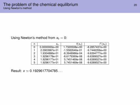
The problem of the chemical equilibrium 20Using Newton’s method
Using Newton’s method from x0 = 0:
n xn f (xn) f ′(xn)0 0.0000000e+00 1.7320508e+00 -8.2857437e+001 2.0903987e-01 -1.5582646e-01 -9.7446356e+002 1.9304886e-01 -8.3948986e-04 -9.6394777e+003 1.9296178e-01 -8.6179369e-08 -9.6389027e+004 1.9296177e-01 5.7451469e-08 -9.6389027e+005 1.9296177e-01 5.7451469e-08 -9.6389027e+00
Result: x ' 0.1929617704785 . . .
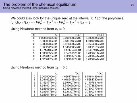
The problem of the chemical equilibrium 21Using Newton’s method (other possible choices)
We could also look for the unique zero at the interval [0, 1] of the polynomialfunction f (x) = (PK 2
p − 1)x3 + (PK 2p − 1)x2 + 5x − 3.
Using Newton’s method from x0 = 0.
n xn f (xn) f ′(xn)0 0.0000000e+00 -3.0000000e+00 5.0000000e+001 6.0000002e-01 2.6391169e+01 1.0946504e+022 3.5890782e-01 6.8148637e+00 5.5594986e+013 2.3632728e-01 1.3453506e+00 3.4332970e+014 1.9714189e-01 1.1747546e-01 2.8407431e+015 1.9300650e-01 1.2435187e-03 2.7806711e+016 1.9296178e-01 1.9213077e-07 2.7800241e+017 1.9296178e-01 1.9213077e-07 2.7800241e+01
Using Newton’s method from x0 = 0.5
n xn f (xn) f ′(xn)0 5.0000000e-01 1.6681749e+01 8.5181496e+011 3.0416229e-01 4.0489445e+00 4.5588730e+012 2.1534771e-01 6.5910071e-01 3.1107981e+013 1.9416019e-01 3.3420280e-02 2.7973827e+014 1.9296549e-01 1.0334284e-04 2.7800777e+015 1.9296178e-01 1.9213077e-07 2.7800241e+016 1.9296178e-01 1.9213077e-07 2.7800241e+01

The problem of the chemical equilibrium 22Using secant method
We look for the unique zero at [0, 1] of the functionf (x) = (1− x)
√3 + x − Kp
√Px√
1 + x , using secant method with x0 = 0and x1 = 1.
n xn f (xn) δf (xn−1, xn)0 0.0000000e+00 1.7320508e+001 1.0000000e+00 -9.6765690e+00 -1.1408620e+012 1.5181950e-01 3.9093074e-01 -1.1869525e+013 1.8475516e-01 7.8879923e-02 -9.4745569e+004 1.9308060e-01 -1.1454452e-03 -9.6121454e+005 1.9296144e-01 3.2173295e-06 -9.6392937e+006 1.9296177e-01 5.7451469e-08 -9.6389017e+007 1.9296177e-01 5.7451469e-08 -9.6389017e+00

Lecture 4 1
Polynomial interpolation

An example: the antifreeze 2Statement of the problem
“Glycerin has lots of uses besides being used to make nitroglycerin. Some uses for glycerin
include: conserving preserved fruit, as a base for lotions, to prevent freezing in hydraulic jacks, to
lubricate molds, in some printing inks, in cake and candy making, and (because it has an antiseptic
quality) sometimes to preserve scientific specimens in jars in your high school biology lab."Goal: We want to estimate the freezing point of an antifreezeconsisting of a solution of glycerin and water at a 45% concentrationlevel in weight.
Data. We have a table of values (taken from previous experiments)with the values of the freezing point (in Celsius degrees) (y ), as afunction of the concentration of glycerin (x).
x 0 10 20 30 40 50 60 70 80 90 100y 0 −1.6 −4.8 −9.5 −15.4 −21.9 −33.6 −37.8 −19.1 −1.6 17
Glycerol: Molecular representation and 3D model showing the atoms and a pair ofelectrons (pink balls) for each oxygen atom.
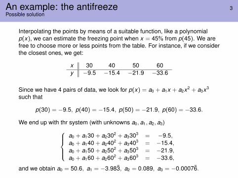
An example: the antifreeze 3Possible solution
Interpolating the points by means of a suitable function, like a polynomialp(x), we can estimate the freezing point when x = 45% from p(45). We arefree to choose more or less points from the table. For instance, if we considerthe closest ones, we get:
x 30 40 50 60y −9.5 −15.4 −21.9 −33.6
Since we have 4 pairs of data, we look for p(x) = a0 + a1x + a2x2 + a3x3
such that
p(30) = −9.5, p(40) = −15.4, p(50) = −21.9, p(60) = −33.6.
We end up with thr system (with unknowns a0, a1, a2, a3)a0 + a130 + a2302 + a3303 = −9.5,a0 + a140 + a2402 + a3403 = −15.4,a0 + a150 + a2502 + a3503 = −21.9,a0 + a160 + a2602 + a3603 = −33.6,
and we obtain a0 = 50.6, a1 = −3.983, a2 = 0.089, a3 = −0.00076.
An example: the antifreeze 4Possible solution
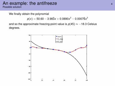
We finally obtain the polynomial
p(x) = 50.60 − 3.983x + 0.0890x2 − 0.00076x3
and so the approximate freezing-point value is p(45) ≈ −18.3 Celsiusdegrees.

An example: the antifreeze 5Possible solution
In the previous plot, we can appreciate that the approximation fails at theends. To improve this failure, there are other interpolation schemes, likesplines:
The interpolating polynomial 6Existence and uniqueness theorem
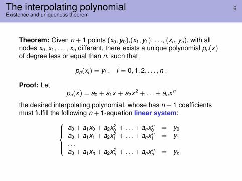
Theorem: Given n + 1 points (x0, y0),(x1, y1), . . ., (xn, yn), with allnodes x0, x1, . . . , xn different, there exists a unique polynomial pn(x)of degree less or equal than n, such that
pn(xi ) = yi , i = 0,1,2, . . . ,n .
Proof: Letpn(x) = a0 + a1x + a2x2 + . . .+ anxn
the desired interpolating polynomial, whose has n + 1 coefficientsmust fulfill the following n + 1-equation linear system:
a0 + a1x0 + a2x20 + . . .+ anxn
0 = y0a0 + a1x1 + a2x2
1 + . . .+ anxn1 = y1
. . .a0 + a1xn + a2x2
n + . . .+ anxnn = yn

The interpolating polynomial 7Existence and uniqueness theorem (end of proof)
The determinant of the system is
∆ =
∣∣∣∣∣∣∣∣1 x0 . . . xn
01 x1 . . . xn
1· · . . . ·1 xn . . . xn
n
∣∣∣∣∣∣∣∣ =n∏
i, j = 0,i > j
(xi − xj ) .
Since ∆ 6= 0 by hypothesis, the system is compatible and determined.Therefore, the problem has a solution and it is unique.
Remark: ∆ is called the Vandermonde determinant.
Remark: The proof also provides a direct (but inefficient) algorithm tocompute the interpolating polynomial.
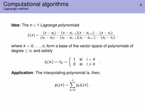
Computational algorithms 8Lagrange method
Idea: The n + 1 Lagrange polynomials
lk (x) =(x − x0) · · · (x − xk−1)(x − xk+1) · · · (x − xn)
(xk − x0) · · · (xk − xk−1)(xk − xk+1) · · · (xk − xn),
where k = 0, . . . ,n, form a base of the vector space of polynomials ofdegree ≤ n, and satisfy
lk (xi ) = δik =
{1 si i = k0 si i 6= k .
Application: The interpolating polynomial is, then,
pn(x) =n∑
k=0
yk lk (x) .

Computational algorithms 9Lagrange method (example)
Example: Consider the following table of values of a function f
x 30 40 50 60y −9.5 −15.4 −21.9 −33.6
We want to estimate f (45) using a polynomial of degree 3.
1) The Lagrange polynomials are:
l0(x) =−1
6000(x − 40)(x − 50)(x − 60) ,
l1(x) =1
2000(x − 30)(x − 50)(x − 60) ,
l2(x) =−1
2000(x − 30)(x − 40)(x − 60) ,
l3(x) =1
6000(x − 30)(x − 40)(x − 50) .
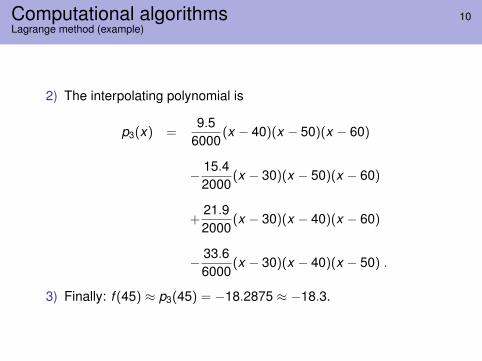
Computational algorithms 10Lagrange method (example)
2) The interpolating polynomial is
p3(x) =9.5
6000(x − 40)(x − 50)(x − 60)
− 15.42000
(x − 30)(x − 50)(x − 60)
+21.92000
(x − 30)(x − 40)(x − 60)
− 33.66000
(x − 30)(x − 40)(x − 50) .
3) Finally: f (45) ≈ p3(45) = −18.2875 ≈ −18.3.

Computational algorithms 11Lagrange method (example)
Question: To extrapolate one result from a table of values, how manynodes do we have to consider?Answer: We can increment the number of nodes since theextrapolated value stabilizes.Remark: It seems reasonable to take more interpolation nodes inorder to improve the estimations. The following example illustratessome inherent problems . . .Example: In order to estimate the valor f (45) corresponding to thefreezing point of the antifreeze at 45% of glycerin:
nodes 40− 50, p1(45) = −18.6500 ≈ −18.7;nodes 30− 60, p3(45) = −18.2875 ≈ −18.3;nodes 20− 70, p5(45) = −18.1457 ≈ −18.1;nodes 10− 80, p7(45) = −18.1234 ≈ −18.1;nodes 00− 90, p9(45) = −18.1363 ≈ −18.1.
Thus, it seems reasonable to approximate f (45) ≈ −18.1.Remark: The value 45 occupies a “central” place within the table.

Computational algorithms 12Lagrange method (example)
Example: In order to estimate the valor f (85) corresponding to thefreezing point of the antifreeze at 85% of glycerin:
nodes 80− 90, p1(85) = −10.35;
nodes 70− 100, p3(85) = −10.3437 . . . ≈ −10.34;
nodes 50− 100, p5(85) = −8.9528 ≈ −8.95;
nodes 30− 100, p7(85) = −7.6172 ≈ −7.62;
nodes 10− 100, p9(85) = −7.1235 ≈ −7.12.

Computational algorithms 13(Newton) Divided differences method
Idea: Express the interpolating polynomial of {(x0, y0), . . . , (xn, yn)} inthe form:
pn(x) = c0 + c1(x − x0) + · · ·+ cn(x − x0)(x − x1) · · · (x − xn−1) .
We have
y0 = pn(x0) = c0
y1 = pn(x1) = c0 + c1(x1 − x0) = y0 + c1(x1 − x0)
y2 = pn(x2) = c0 + c1(x2 − x0) + c2(x2 − x0)(x2 − x1)
. . .
and so
c0 = y0, c1 =y1 − y0
x1 − x0, c2 =
y2−y1x2−x1
− y1−y0x1−x0
x2 − x0, . . .

Computational algorithms 14(Newton) Divided differences method
We compute divided differences
x0 f [x0] = y0 = c0
f [x0, x1] = f [x1]−f [x0]x1−x0
= c1
x1 f [x1] = y1 f [x0, x1, x2] = f [x1,x2]−f [x0,x1]x2−x0
= c3
f [x1, x2] = f [x2]−f [x1]x2−x1
x2 f [x2] = y2...
...... . . .
...... f [xn−1, xn] =
f [xn ]−f [xn−1]
xn−xn−1
xn f [xn] = yn
Then: cj = f [x0, x1, . . . , xj ] per j = 0,1, . . . ,n.

Computational algorithms 15(Newton) Divided differences method (example)
Example: Consider the following table of values of a function f
x 30 40 50 60y −9.5 −15.4 −21.9 −33.6
We want to estimate f (45) using a polynomial of degree 3.
1) The table of divided differences is
30 −9.5−15.4+9.5
40−30 =−0.5940 −15.4 −0.65+0.59
50−30 =−0.003−21.9+15.4
50−40 =−0.65 −0.026+0.00360−30 =−0.00076
50 −21.9 −1.17+0.6560−40 =−0.026
−33.6+21.960−50 =−1.17
60 −33.6

Computational algorithms 16(Newton) Divided differences method (example)
2) The interpolating polynomial, p3(x), is
p3(x) = −9.5− 0.59(x − 30)
−0.003(x − 30)(x − 40)
−0.00076(x − 30)(x − 40)(x − 50) .
3) Finally: f (45) ≈ p3(45) = −18.2875.
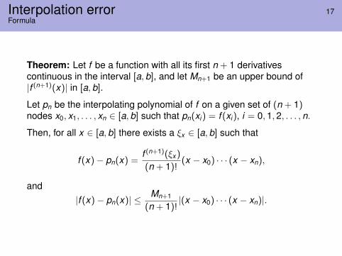
Interpolation error 17Formula
Theorem: Let f be a function with all its first n + 1 derivativescontinuous in the interval [a,b], and let Mn+1 be an upper bound of|f (n+1)(x)| in [a,b].
Let pn be the interpolating polynomial of f on a given set of (n + 1)nodes x0, x1, . . . , xn ∈ [a,b] such that pn(xi ) = f (xi ), i = 0,1,2, . . . ,n.
Then, for all x ∈ [a,b] there exists a ξx ∈ [a,b] such that
f (x)− pn(x) =f (n+1)(ξx )
(n + 1)!(x − x0) · · · (x − xn),
and|f (x)− pn(x)| ≤ Mn+1
(n + 1)!|(x − x0) · · · (x − xn)|.
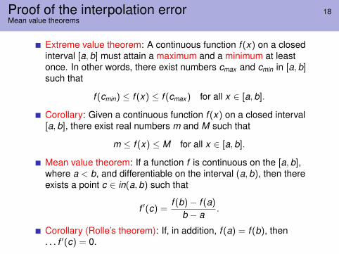
Proof of the interpolation error 18Mean value theorems
Extreme value theorem: A continuous function f (x) on a closedinterval [a,b] must attain a maximum and a minimum at leastonce. In other words, there exist numbers cmax and cmin in [a,b]such that
f (cmin) ≤ f (x) ≤ f (cmax ) for all x ∈ [a,b].
Corollary: Given a continuous function f (x) on a closed interval[a,b], there exist real numbers m and M such that
m ≤ f (x) ≤ M for all x ∈ [a,b].
Mean value theorem: If a function f is continuous on the [a,b],where a < b, and differentiable on the interval (a,b), then thereexists a point c ∈ in(a,b) such that
f ′(c) =f (b)− f (a)
b − a.
Corollary (Rolle’s theorem): If, in addition, f (a) = f (b), then. . . f ′(c) = 0.
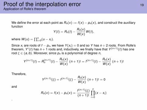
Proof of the interpolation error 19Application of Rolle’s theorem
We define the error at each point as Rn(x) := f (x)− pn(x), and construct the auxiliaryfunction
Y (t) = Rn(t)−Rn(x)W (x)
W (t),
where W (u) =∏n
i=0(u − xi ).
Since xi are roots of f − pn, we have Y (xi ) = 0 and so Y has n + 2 roots. From Rolle’stheorem, Y ′(t) has n + 1 roots and, inductively, we finally have that Y (n+1)(t) has oneroot ξ ∈ (a, b). Moreover, since pn is a polynomial of degree n,
Y (n+1)(t) = R(n+1)n (t)−
Rn(x)W (x)
(n + 1)! = f (n+1)(t)−Rn(x)W (x)
(n + 1)!
Therefore,
Y (n+1)(ξ) = f (n+1)(ξ)−Rn(x)W (x)
(n + 1)! = 0
and
Rn(x) = f (x)− pn(x) =f (n+1)(ξ)
(n + 1)!
n∏i=0
(x − xi )
.

Interpolation error: f (x)− pn(x) =f (n+1)(ξx )
(n+1)! (x − x0) · · · (x − xn), 20Remarks
1 The error at the interpolation nodes is zero.2 If f (x) is a polynomial of degree n, the error is zero everywhere.3 General bounds:
If a = x0 ≤ x1 ≤ . . . ≤ xn = b, and |f (n+1)(x)| ≤ Mn+1 for allx ∈ [a,b], then:
|f (x)− pn(x)| ≤ Mn+1
(n + 1)!(b − a)n+1 .
4 Specific bounds (equally spaced nodes):If xi = x0 + i · h for i = 0,1, . . . ,n, with h = (b−a)
n , and|f (n+1)(x)| ≤ Mn+1 for all x ∈ [a,b], then:
|f (x)− pn(x)| ≤ Mn+1
4(n + 1)
(b − a
n
)n+1
.

Interpolation error 21Example
Example: We interpolate the functions sinus and cosinus in theinterval [0, π2 ] for a polynomial of degree 6, using equally spacesnodes. Which is the truncating error?
Solution: Both for f (x) = sin x and f (x) = cos x , we can bound anyderivative (in particular, the 7th one) by 1. Then, at any pointx ∈ [0, π2 ], we can bound the truncating error by
|f (x)− p6(x)| ≤ 14 · 7
(π/26
)7
≤ 3.02 · 10−6 .
Exercise: How many equally spaced nodes (and so, which degree ofthe interpolating polynomial) are needed for the truncating error atany point in the interval [0, π2 ] to be less than 10−10?
Answer: 11 nodes (degree 10) since the value of 14(n+1)
(π2n
)(n+1) for n = 9 is still oforder 10−9 but for n = 10 it is 0.3x10⁻¹⁰.

Runge’s phenomenon 22A surprising feature
Question: Does the approximation obtained with the interpolatingpolynomial improves when we increase the number of nodes (and sothe degree of pn)?
Example: (C. Runge(1901)) Let pn(x) the interpolating polynomial ofthe function
f (x) =1
1 + 25x2 , x ∈ [−1,1],
on the set of equally spaced points xi = −1 + 2in , i = 0,1, . . . ,n.
Then, if 0.726 . . . ≤ |x | < 1, supn≥0 |f (x)− pn(x)| =∞.
Remark: The error near the origin is small but nearby −1 and 1 itgrows with n.

Runge’s phenomenon 23Graphics
We observe the function f (x) = 1/(1 + 25x2) and its interpolatingpolynomials of degrees 4, 8 and 12.

Lecture 5 1
Taylor polynomials and powerseries

An example: real gases 2The virial equation of state
Example: The virial 1expansion or virial series of a gas is its stateequation in the form
Z :=PVnRT
= 1 + B2(T )( n
V
)+ B3(T )
( nV
)2+ . . .
where P is the pressure, V is the volume, T is the absolutetemperature, n is the number of moles, and R ' 8.3145 J K−1mol−1
is the ideal gas constant.
Z is the compressibility factor (for an ideal gas, Z = 1).
The addends are successive corrections to the ideal case, andcorrespond to intramolecular forces between pairs (B2(T )), triplets(B3(T )), and so on.
Other forms of the virial equation use the molar volumeV = Vm := V/n or the molar density ρ := n/V . In the latter 2,
PRT
= ρ+ B2(T )ρ2 + B3(T )ρ3 + . . . .
1From latin, “virial” means “force”. Here refers the fact that gases are not ideal sincethere are intramolecular forces.
2The equation was proposed in 1901 by the Nobel laureate Heike KamerlinghOnnes (1853-1926).
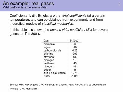
An example: real gases 3Virial coefficients: experimental data
Coefficients 1, B2, B3, etc. are the virial coefficients (at a certaintemperature), and can be obtained from experiments and fromtheoretical models of statistical mechanics.
In this table it is shown the second virial coefficient (B2) for severalgases, at T = 300 K.
Gas B2(300)ammonia -265argon -16carbon dioxide -126chlorine -299ethylene -139hidrogen 15methane -43nitrogen -4oxigen -16sulfur hexafluoride -275water -1126
Source: W.M. Haynes (ed.) CRC Handbook of Chemistry and Physics, 97a ed., Boca Raton
(Florida), CRC Press 2016.

An example: real gases 4Van der Waals equation of state
Problem: How can we compute the virial expansion from a givenstate equation, obtained theoretically from the intramolecularpotential of a gas?
An important example is the Van der Waals equation of state:(P + a
( nV
)2)
(V − nb) = nRT ,
where a and b are gas dependent constants.
The second virial coefficient B2(T ) is the most important, since it isthe main correction term.
The Boyle temperature is the temperature for which the second virialcoefficient is zero, that is TB such that B2(TB) = 0. At thistemperature, the gas behaves as if it were ideal.
Problem: Which is the Boyle temperature for the Van der Waalsequation of state?
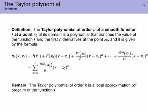
The Taylor polynomial 5Definition
Definition: The Taylor polynomial of order n of a smooth functionf at a point x0 of its domain is a polynomial that matches the value ofthe function f and the first n derivatives at the point x0, and it is givenby the formula:
pn(x , x0) = f (x0) + f ′(x0)(x − x0) +f ′′(x0)
2!(x − x0)2 + · · ·+ f (n)(x0)
n!(x − x0)n
=n∑
k=0
f (k)(x0)
k !(x − x0)k .
Remark: The Taylor polynomial of order n is a local approximation (oforder n) of the function f .
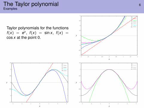
The Taylor polynomial 6Examples
Taylor polynomials for the functionsf (x) = ex , f (x) = sin x , f (x) =cos x at the point 0.

Taylor’s theorem 7Lagrange form of the remainder
Theorem: Let f :]a,b[→ R be a (n + 1) times differentiable function,and x0 ∈]a,b[. Let
rn(x , x0) = f (x)− pn(x , x0)
be the remainder or truncation error at a point x ∈]a,b[. Then, thereexists ξx ∈]x0, x [ such that
rn(x , x0) =f (n+1)(ξx )
(n + 1)!(x − x0)n+1.

Taylor’s theorem 8An application in evaluation of functions
Example: We want to approximate sine and cosine functions usingtheir Taylor polynomials of order 6, centered at 0. We also want toestimate the truncation error for any x ∈ [0, π/2].
For the sine function, we have
ps6(x) = x − 1
3!x3 +
15!
x5,
and the remainder is
|r s6 (x)| =
| − cos(ξs)|7!
x7 ≤ 17!
x7.
For the cosine function, we have
pc6(x) = 1− 1
2!x2 +
14!
x4 − 16!
x6,
and the remainder is
|r c6 (x)| =
| sin(ξc)|7!
x7 ≤ 17!
x7.

Taylor’s theorem 9An application in computer approximations of functions
For x ∈ [0, π/2], we obtain the following bound for the remainders, inboth the sine and cosine cases:
17!
(π2
)7≤ 0.47 · 10−2.
Question: What is the order we have to reach in such a way that thetruncation error is smaller than 10−10? Answer: 15.

Power series 10Definition
If we “take” n =∞ in the definition of the Taylor polynomial, we get
S(f )(x , x0) =∞∑
k=0
f (k)(x0)
k !(x − x0)k ,
which is the Taylor series or the power series of the function f at thepoint x0.
Remark: In order that f (x) = S(f )(x , x0), the remainder rn(x , x0) hasto go to zero when n goes to +∞. A convergence criteria for generalpower series
S(f )(x , x0) =∞∑
k=0
ak (x − x0)k ,
is as follows:
If limk→∞
∣∣∣∣ ak
ak+1
∣∣∣∣ = R, the series S(f )(x , x0) converges for x s.t.
|x − x0| < R.
In the Taylor case, ak =f (k)(x0)
k !, and a posteriori S(f )(x , x0) = f (x)
for x s.t. |x − x0| < R.

Power series 11Taylor series of some elementary functions
11− x
=∞∑
n=0
xn = 1 + x + x2 + x3 + · · · , − 1 < x < 1
(1 + x)α =∞∑
n=0
(αn
)xn = 1 + αx +
α(α− 1)2!
x2 + · · · , α ∈ R, − 1 < x < 1
ex =∞∑
n=0
xn
n!= 1 + x +
x2
2!+
x3
3!+ · · · , −∞ < x <∞
sin x =∞∑
n=0
(−1)n x2n+1
(2n + 1)!= x −
x3
3!+
x5
5!−
x7
7!+ · · · , −∞ < x <∞
cos x =∞∑
n=0
(−1)n x2n
(2n)!= 1−
x2
2!+
x4
4!−
x6
6!+ · · · , −∞ < x <∞
ln(1− x) =∞∑
n=1
−1n
xn = −x −x2
2−
x3
3−
x4
4+ · · · , − 1 < x < 1
ln(1 + x) =∞∑
n=1
(−1)n+1
nxn = x −
x2
2+
x3
3−
x4
4+ · · · , − 1 < x < 1
n! = 1 · 2 · · · · · n,(αn
)=α(α− 1) . . . (α− n + 1)
n!

Power series 12The geometric series
Example: Compute the power series (at x0 = 0) of the function
f (x) =1
1− x= (1− x)−1.
Solution: We have that
f (k)(x) = k !(1− x)−k−1.
Therefore, f (k)(0) = k ! and
S(f )(x) =∞∑
k=0
k !
k !xk =
∞∑k=0
xk = 1 + x + x2 + . . .
The formula works for −1 < x < 1.

Power series 13The geometric series
x 0.2 -0.5 2f (x) 1.25 0.6 -1
p0(x) 1.00000000 1.00000000 1p1(x) 1.20000000 5.00000000E-001 3p2(x) 1.24000000 7.50000000E-001 7p3(x) 1.24800000 6.25000000E-001 15p4(x) 1.24960000 6.87500000E-001 31p5(x) 1.24992000 6.56250000E-001 63p6(x) 1.24998400 6.71875000E-001 127p7(x) 1.24999680 6.64062500E-001 255p8(x) 1.24999936 6.67968750E-001 511p9(x) 1.24999988 6.66015625E-001 1023p10(x) 1.24999998 6.66992188E-001 2047p11(x) 1.25000000 6.66503906E-001 4095p12(x) 1.25000000 6.66748047E-001 8191p13(x) 1.25000000 6.66625977E-001 16383p14(x) 1.25000000 6.66687012E-001 32767p15(x) 1.25000000 6.66656494E-001 65535
Question: Which is the series for x = 1/2?

Power series 14Manipulation
We can do algebraic operations with power series, as well ascompose, compute derivatives and integrals.
Example 1: We want to compute the power series of the function
f (x) =1
1− 8x3 .
Solution: Define y = 8x3. We know that, for −1 < y < 1,
11− y
=∞∑
k=0
yk .
Hence, if −12< x <
12
11− 8x3 =
∞∑k=0
(8x3)k =∞∑
k=0
8k x3k = 1 + 8x3 + 82x6 + . . .

Power series 15Manipulation
Exemple 2: We want to compute the power series of the function
f (x) =12
log(
1 + x1− x
).
Solution 1: The series of log(1 + x) and log(1− x) work for−1 < x < 1, and subtracting them and dividing by 2 we obtain:
12
log(
1 + x1− x
)= x +
x3
3+
x5
5+
x7
7+ . . .
Solution 2: Differentiating f (x), we obtain f ′(x) =1
1− x2 , and,
hence,f ′(x) = 1 + x2 + x4 + . . .
at the interval −1 < x < 1. By integrating the series (term by term)from 0 to x , and taking into account that f (0) = 0, we reach the samesolution.
Application: To compute log z for any z > 0, one can compute firstx ∈]− 1,1[ such that z = 1+x
1−x , that is x = z−1z+1 , and apply the previous
formula.

Applications 16Van der Waals state equation and virial coefficients
Problem: Find the virial series of Van der Waals equation(P + a
( nV
)2)
(V − nb) = nRT ,
and Boyle’s temperature.
Solution: We have to expand with respect to the molar densityρ = n/V the compressibility factor Z :
Z =PVnRT
=1
1− b nV− a
RT
( nV
)=
11− bρ
− aRT
ρ.
If −1 < bρ < 1, then:
Z = 1 +(
b − aRT
)ρ+ b2ρ2 + b3ρ3 + · · · .
In particular B2(T ) =∂Z∂ρ |ρ=0
=(
b − aRT
)Boyle temperature is TB =
aRb
.

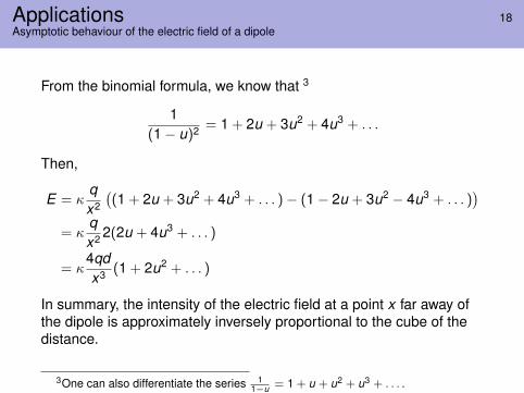
Applications 17Asymptotic behaviour of the electric field of a dipole
Problem: Given a dipole with charges q i −q, at distance 2d of eachother, what is the order of magnitude of the electric field of thecorresponding dipole far away in a point in the axis?
Solution: If the charges q,−q are at points d ,−d , respectively, of Xaxis, the intensity of electric field generated by the dipole at a point xon the axis is
E = κ
(q
(x − d)2 −q
(x + d)2
).
By hypothesis, x � d . By defining u = dx � 1, we have
E = κqx2
(1
(1− u)2 −1
(1 + u)2
).
Applications 18Asymptotic behaviour of the electric field of a dipole
From the binomial formula, we know that 3
1(1− u)2 = 1 + 2u + 3u2 + 4u3 + . . .
Then,
E = κqx2
((1 + 2u + 3u2 + 4u3 + . . . )− (1− 2u + 3u2 − 4u3 + . . . )
)= κ
qx2 2(2u + 4u3 + . . . )
= κ4qdx3 (1 + 2u2 + . . . )
In summary, the intensity of the electric field at a point x far away ofthe dipole is approximately inversely proportional to the cube of thedistance.
3One can also differentiate the series 11−u = 1 + u + u2 + u3 + . . . .
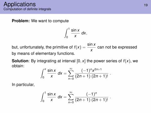
Applications 19Computation of definite integrals
Problem: We want to compute∫ 1
0
sin xx
dx ,
but, unfortunately, the primitive of f (x) =sin x
xcan not be expressed
by means of elementary functions.
Solution: By integrating at interval [0, x ] the power series of f (x), weobtain: ∫ x
0
sin xx
dx =∞∑
n=0
(−1)nx2n+1
(2n + 1) (2n + 1)!.
In particular, ∫ 1
0
sin xx
dx =∞∑
n=0
(−1)n
(2n + 1) (2n + 1)!.

Lecture 6 1
Integration in one variable

An example: area under glucose curve 2
Recordings of glucose levels are performed in diabetes control to getinformation about an individual’s glucose tolerance. It is commonpractice to use simple summary measures: fasting value, two-hour (2-h)value or area under the curve (AUC),. . . .
t 0 30 60 90 120y 4.00 5.77 5.27 4.12 2.98
Table shows OGTTs (oral glucose tolerance tests)
with 5 glucose measurements over two hours
recorded for healthy pregnant women in their first
trimester (averages over population).
Goal: Compute the area under thecurve.
1008060400 20 1202.5
3
3.5
4
4.5
5
5.5
6
Time (min)
Glu
cose
con
cent
ratio
n (m
mol
/ l)
Glucose "curve"

An example: area under glucose curve 3
Recordings of glucose levels are performed in diabetes control to getinformation about an individual’s glucose tolerance. It is commonpractice to use simple summary measures: fasting value, two-hour (2-h)value or area under the curve (AUC),. . . .
t 0 30 60 90 120y 4.00 5.77 5.27 4.12 2.98
Table shows OGTTs (oral glucose tolerance tests)
with 5 glucose measurements over two hours
recorded for healthy pregnant women in their first
trimester (averages over population).
Goal: Compute the area under thecurve.
120100802.5
3
3.5
4
4.5
5
5.5
6
Time (min)
Glu
cose
con
cent
ratio
n (m
mol
/ l)
Glucose "curve"
6040200
An example: area under glucose curve 4
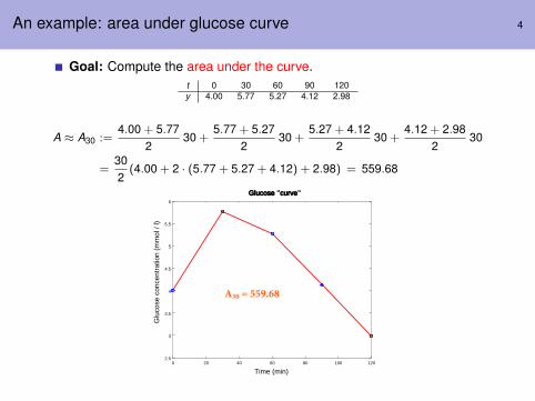
Goal: Compute the area under the curve.t 0 30 60 90 120y 4.00 5.77 5.27 4.12 2.98
A ≈ A30 :=4.00 + 5.77
230 +
5.77 + 5.272
30 +5.27 + 4.12
230 +
4.12 + 2.982
30
=302(4.00 + 2 · (5.77 + 5.27 + 4.12) + 2.98) = 559.68
120100802.5
3
3.5
4
4.5
5
5.5
6
Time (min)
Glu
cose
con
cent
ratio
n (m
mol
/ l)
Glucose "curve"
6040200
A30 = 559.68

An example: area under glucose curve 5
Assume that you have a non-invasive way to record glucose levels andyou can take more measurements.
t 0 10 20 30 40 50 60 70 80 90 100 110 120y 4.00 5.02 5.56 5.77 5.75 5.56 5.27 4.91 4.52 4.12 3.73 3.34 2.98
Table shows OGTTs (oral glucose tolerance tests)
with 13 glucose measurements over two hours
recorded for healthy pregnant women in their first
trimester (averages over population).
5
5.5
6
Time (min)
Glu
cose
con
cent
ratio
n (m
mol
/ l)
Glucose "curve"
4.5
4
3.5
3
2.5120100806040200

An example: area under glucose curve 6
Goal: Compute the area under the curve.t 0 10 20 30 40 50 60 70 80 90 100 110 120y 4.00 5.02 5.56 5.77 5.75 5.56 5.27 4.91 4.52 4.12 3.73 3.34 2.98
A ≈ A10 :=10
2(4.00 + 2 · (5.02 + 5.56 + 5.77 + 5.75 + 5.56 + 5.27 + 4.91+
4.52 + 4.12 + 3.73 + 3.34) + 2.98) = 570.47
5
5.5
6
Time (min)
Glu
cose
con
cent
ratio
n (m
mol
/ l)
Glucose "curve"
4.5
4
3.5
3
2.5120100806040200
A10=570.47

An example: area under glucose curve 7
Heuristics: If we could take infinitely many measurements, we could get thearea under the curve through a limiting process, taking finer partitions of theinterval.
The area under the curve, defined with the limiting process, is the definiteintegral
A =
∫ 120
0y(t) dt .
In fact, the values of the table have an excellent fitwith the function
y(t) = (a + bt) exp(−ct)
where
a ' 4.0014, b ' 0.20549, c ' 0.018858.
The area is A ' 571.77. 2.5
3
3.5
4
4.5
5
5.5
6
0 20 40 60 80 100 120
"glucose.dat"
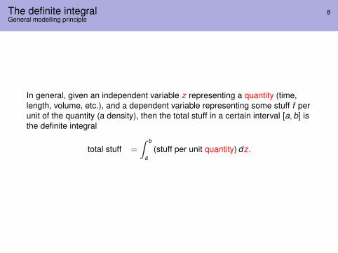
The definite integral 8General modelling principle
In general, given an independent variable z representing a quantity (time,length, volume, etc.), and a dependent variable representing some stuff f perunit of the quantity (a density), then the total stuff in a certain interval [a, b] isthe definite integral
total stuff =
∫ b
a(stuff per unit quantity) dz.
The definite integral 9Upper and lower sums
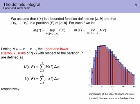
We assume that f (x) is a bounded function defined on [a, b] and that{x0, . . . , xn} is a partition (P) of [a, b]. For each i we let
Mi (f ) = supx∈[xi−1,xi ]
f (x), mi (f ) = infx∈[xi−1,xi ]
f (x).
Letting ∆xi = xi − xi−1, the upper and lower(Darboux) sums of f (x) with respect to the partition Pare defined as
U(f ,P) =n∑
i=1
Mi (f ) ∆xi ,
L(f ,P) =n∑
i=1
mi (f ) ∆xi ,
respectively.Comparison of the upper (blueish) and lower
(reddish) Riemann sums for a fixed partition.
The definite integral 10Definition
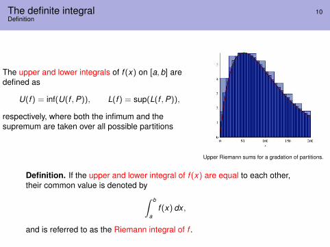
The upper and lower integrals of f (x) on [a, b] aredefined as
U(f ) = inf(U(f ,P)), L(f ) = sup(L(f ,P)),
respectively, where both the infimum and thesupremum are taken over all possible partitions
Upper Riemann sums for a gradation of partitions.
Definition. If the upper and lower integral of f (x) are equal to each other,their common value is denoted by∫ b
af (x) dx ,
and is referred to as the Riemann integral of f .

The definite integral 11Examples
Example 1: ∫ 1
0x2 dx
Take ∆ x = 1/n:
1n
n−1∑k=0
(kn
)2
≤∫ 1
0x2 dx ≤ 1
n
n∑k=1
(kn
)2
From Problem 2 in Exam Model, we know thatn∑
k=1k2 = 1
3 n3 + 12 n2 + 1
6 n, so:
1n3
(13(n − 1)3 +
12(n − 1)2 +
16(n − 1)
)≤∫ 1
0x2 dx ≤
1n3
(13
n3 +12
n2 +16
n).
Since both sides of the inequality tend to 13 when n goes to∞, then∫ 1
0x2 dx =
13.

The definite integral 12Examples
Example 2: [Ledder, Example 1.7.6.]Goal and strategy:
We want to relate the birth rate of a population with survival andfecundity data in a female population.We will calculate the birth rate at time t by adding up the births tomothers of various ages.
Ingredients:B(t) is the birth rate at time t .Take all possible mothers of age in [a, a + da]. Observe that they wereborn when the birth rate was B(t − a). So, the initial size of this cohortwas B(t − a) da.Let `(a) be the fraction of individuals who survive to age a or greater.Then, the size of the age-a cohort is `(a) B(t − a) da.Let a ∈ [a1, a2], the age-interval of fertility and m(a) be the rate of birthsper capita for age-a individuals. Then the total rate of births for mothersof age a is m(a) `(a) B(t − a) da.
Thus, the birth rate satisfies the equation
B(t) =
∫ a2
a1
m(a) `(a) B(t − a) da.

The definite integral 13Examples
Example 3: [Ledder, Example 1.7.7.]Goal and strategy:
A population of microorganisms is distributed along a stream of length10 with linear density 1000 e−0.1x individuals per unit length.
We aim at computing the the total number p of individuals in the stream.
Ingredients:The number of individuals associated in an infinitesimal portion of thestream [x , x + dx ] is 1000 e−0.1 x dx .
Thus,
p =
∫ 10
01000 e−0.1 x dx .

The definite integral 14Properties
Linearity rule. Let a, b, A, and B be any constants. If thefunctions f and g have integrals on the interval [a, b], then∫ b
a[Af (x) + Bg(x)] dx = A
∫ b
af (x) dx + B
∫ b
ag(x) dx .
Partition rule. If the function f has integrals on the intervals[a, b] and [b, c], then∫ c
af (x) dx =
∫ b
af (x) dx +
∫ c
bf (x) dx .

Riemann integrable functions 15Important results
We have the following important results.
Let f : [a, b]→ R be a bounded function.
If f is monotone (increasing or decreasing), then it is Riemann integrablein [a, b].
If f is continuous, then it is Riemann integrable in [a, b].
If f is Riemann integrable in [a, b], with f ([a, b]) ⊂ [c, d ], andg : [c, d ]→ R is continuous, then g ◦ f is Riemann integrable in [a, b].
Warning! Not all bounded functions are Riemann integrable. For instance,the function f : R→ R defined by
f (x) =
{1 if x /∈ Q0 if x ∈ Q
,
is not Riemann integrable in any interval [a, b].

The fundamental theorem of calculus 16Motivation and first statement
Motivation. x(b)− x(a) =∫ b
a v(t) dt since ∆ x ≈ v(t) ∆ t .
Statement (first “issue"). Suppose F ′ is continuous on the interval[a, b]. Then, ∫ b
aF ′(t) dt = F (b)− F (a).
In every accumulation problem, we express the total change in a quantity as the integral of the rate of change.
Example. ∫ π
0sin x dx = −cosπ + cos 0 = −(−1) + 1 = 2
taking f (x) = − cos x and so f ′(x) = sin x as desired.

The fundamental theorem of calculusStatement and sketch proof
Theorem. Let f : [a, b]→ R be a continuous function. Define F : [a, b]→ Ras
F (x) =
∫ x
af (z) dz.
Then F is continuously differentiable, and F ′ = f .
Sketch of the proof. Notice that
F ′(x) = limh→0
F (x + h)− F (x)
h= lim
h→0
1h
∫ x+h
xf (z) dz
and that, in [x , x + h], ∫ x+h
xf (z) dz ' f (x)h.
The fundamental theorem of calculusBarrow’s rule
Definition: It is said that F , defined as F (x) =∫ x
a f (z) dz, is a primitive orantiderivative of f . A primitive of f is defined up to an additive constant. Theset of all primitives of f is its indefinite integral, denoted by
∫f (x) dx . Hence,
we have: ∫f (x) dx = F (x) + C.
Corollary [Barrow’s rule] Let f : [a, b]→ R be a continuous function, andg : [a, b]→ R a primitive of f . Then:∫ b
af (x) dx = [g(x)]b
a := g(b)− g(a).

Computation of antiderivatives/primitives 19Elementary integrals
Table of elementary integrals (antiderivatives/primitives) (justflipping the table of derivatives).
f ′(x) x r (r 6= −1)1
xea x cos a x sin a x
1
a2 + x2
1√a2 − x2
f (x)x r+1
r + 1log |x|
1
aea x 1
asin a x −
1
acos a x
1
aarctan
x
aarcsin
x
a
Example.∫
(x2 + 1) dx = 13 x3 + x + C.
Exercise. Using a double-angle trigonometric formula, compute∫2 sin x cos x dx .
Exercise. Check that∫
2 sin x cos x dx = sin2 x + C, but also∫2 sin x cos x dx = − cos2 x + C. Why?
Exercise. The functions sinh x = 12
(ex − e−x) and cosh = 1
2
(ex + e−x) are
the hyperbolic sine and cosine functions. Compute their primitives.

Computation of antiderivatives/primitives 20Change of variables (substitution)
Change of variables (substitution).
If f is differentiable and g is continuous with G as a primitive, then, by thechain rule, G(f (x)) is a primitive of g(f (x))f ′(x).
This is often written as∫g(f (x))f ′(x) dx =
∫g(f (x)) df (x) =
∫g(y)dy , y = f (x),
and it is said that the change of variable y = f (x) is performed.

Computation of antiderivatives/primitives 21Change of variables (substitution)
Change of variables (substitution).
∫g(f (x))f ′(x) dx =
∫g(f (x)) df (x) =
∫g(y)dy , where y = f (x).
Example.∫
sin(f (x))f ′(x) dx = − cos(f (x)) + C,∫cos(f (x))f ′(x) dx = sin(f (x)) + C.
Example.∫
f ′(x)
f (x)dx = log |f (x)|+ C.
Example.∫
x√
2x2 + 1 dx =
∫ √y
4dy , with y = 2x2 + 1. Then,∫
x√
2x2 + 1 dx =16
y3/2 + C =16
(2x2 + 1)3/2 + C.
Exercise. Compute: (a)∫
x sin(x2) dx ; (b)∫
log xx
dx .
Computation of antiderivatives/primitives 22Integration by parts
Integration by parts.
If F ,G are two primitives of f , g respectively, then, by Leibniz rule of thederivative of the product, (FG)′ = fG + Fg, so that Fg = (FG)′ − fG. Then,∫
F (x)g(x) dx = F (x)G(x)−∫
f (x)G(x) dx .
A usual way of writing the formula is∫udv = uv −
∫vdu, where du = u′dx , dv = v ′dx .
Example.∫
x sin x dx = −x cos x +∫
cos x dx = −x cos x + sin x + C.
Example.∫
log x dx =∫
1 · log x dx = x log x −∫
x 1x dx = x log x − x + C.
Example.∫
x2ex dx = x2ex −∫
2xex dx = x2ex −(2xex −
∫2ex dx
)=
x2ex − 2xex + 2ex + C = (x2 − 2x + 2)ex .
Exercise. Write an algorithm to compute∫
p(x)ex dx , where p(x) is apolynomial.
Exercise. Compute∫
ex sin x dx by integrating by parts two times.

Computation of antiderivatives/primitives 23Some generalities
The art of computing primitives is based on the previous two methods. Theidea is simply get a suitable change of variable or performing integration byparts, so that the following integral is simpler and reduced to one we cansolve. With these methods, one can compute explicitly the primitives of thefollowing functions:
p(x)eax , p(x) sin(ax), p(x) cos(ax), p(x) log(x), p(x) arctan(x) (p(x) isa polynomial);eax sin(bx), eax cos(bx);
rational functions p(x)q(x) , where p(x), q(x) are polynomials;
trigonometric rational functions R(sin x , cos x), where R(s, c) is arational function in the variables s, c;(some) irrational functions;functions with square roots of polynomials.
There are implementations of these methodologies, based on symboliccalculus.
Unfortunately, there are much more functions for which one can not obtain anexplicit formula for the primitive. Some simple examples are the apparentlynaive functions e−x2
, sin x2 or 1x sin x .
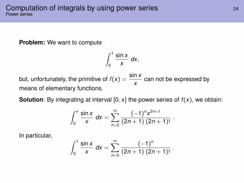
Computation of integrals by using power series 24Power series
Problem: We want to compute ∫ 1
0
sin xx
dx ,
but, unfortunately, the primitive of f (x) =sin x
xcan not be expressed by
means of elementary functions.
Solution: By integrating at interval [0, x ] the power series of f (x), we obtain:∫ x
0
sin xx
dx =∞∑
n=0
(−1)nx2n+1
(2n + 1) (2n + 1)!.
In particular, ∫ 1
0
sin xx
dx =∞∑
n=0
(−1)n
(2n + 1) (2n + 1)!.

Numerical integration 25Introduction
Problem: We aim at computing the integral of a function f in an interval[a, b]. . . but several restrictions may arise:
we have the expression of f , but we are not able to explicitly compute aprimitive; or,
we do not have the expression of f , but we have a recipe to evaluate it; or
we have a table of values of f (most likely, coming from experimentaldata).
Then, we can approximate the integral by means of some numericalintegration formula.
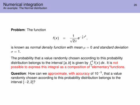
Numerical integration 26An example: The Normal distribution
Problem: The function
f (x) =1√2π
e−12 x2,
is known as normal density function with mean µ = 0 and standard deviationσ = 1.
The probability that a value randomly chosen according to this probabilitydistribution belongs to the interval [a, b] is given by
∫ ba f (x) dx . It is not
possible to express this integral as a composition of “elementary"functions.
Question: How can we approximate, with accuracy of 10−5, that a valuerandomly chosen according to this probability distribution belongs to theinterval [−2, 2]?

Numerical integration 27Basic ideas
Problem: Numerical computation of the integral defined by a function f in aninterval [a, b],
I(f ) =
∫ b
af (x)dx ,≈
n∑i=1
ci f (xi ) for some ci ∈ R
either from the mathematical expression of f or from a table of values of f .Basic ideas:
Approximate f by a polynomial p, and take
I(f ) ≈∫ b
ap(x)dx .
(simple numerical integration formulas).
Divide the interval [a, b] in subintervals, and use the simple numericalintegration formulas in each of the subintervals.(composite numerical integration formulas).

Simple numerical integration formulas 28Some interpolating formulas
In order to estimate the value of I(f ) from the values of f at points a, b andc = 1
2 (a + b), we can use:
Rectangle rule: Approximating f by the constant f (c) we get
I(f ) ≈ IR(f ) = (b − a)f (c) .
Trapezoid rule: Approximating f by the straight line through (a, f (a))and (b, f (b)), we get
I(f ) ≈ IT (f ) =(b − a)
2(f (a) + f (b)) .
Simpson’s formula: Approximating f by the parabola through the points(a, f (a)), (c, f (c)) and (b, f (b)), we get
I(f ) ≈ IS(f ) =b − a
6(f (a) + 4f (c) + f (b)) =
c − a3
(f (a) + 4f (c) + f (b)) .

Composite numerical integration formulas 29Some interpolating formulas
Dividing the interval [a, b] in subintervals, we can apply the simple formulas ineach of them: we choose the nodes {xi = a + ih}n
i=0, on h = b−an .
Composite rectangle rule. If yi = 12 (xi−1 + xi ):
IR(f , h) = h(f (y1) + f (y2) + f (y3) + · · ·+ f (yn−1) + f (yn)).
Composite trapezoid rule:
IT (f , h) =h2
(f (x0) + 2f (x1) + 2f (x2) + · · ·+ 2f (xn−1) + f (xn)).
Composite Simpson’s formula. If n is even, we can apply Simpson’srule to the intervals [x0, x2], [x2, x4], ..., [xn−2, xn]:
IS(f , h) =h3
(f (x0)+4f (x1)+2f (x2)+4f (x3)+· · ·+2f (xn−2)+4f (xn−1)+f (xn)).

Composite numerical integration formulas 30Geometrical idea
Approximation by rectangles Approximation by trapezoids

Composite numerical integration formulas 31Example
Example: Computation of∫ 2
0sin(x2) dx
n Rectangles Trapezoids Simpson2 1.025477156142 0.463069737154 0.8696938146414 0.837368896902 0.744273446648 0.8380080164808 0.811881955543 0.790821171775 0.806337080151
16 0.806496669270 0.801351563659 0.80486169428732 0.805203153963 0.803924116465 0.80478163406764 0.804882946231 0.804563635214 0.804776808130128 0.804803090517 0.804723290722 0.804776509225256 0.804783138822 0.804763190620 0.804776490586512 0.804778151662 0.804773164721 0.804776489421
1024 0.804776904920 0.804775658192 0.8047764893492048 0.804776593238 0.804776281556 0.8047764893444096 0.804776515317 0.804776437397 0.8047764893448192 0.804776495837 0.804776476357 0.804776489344
16384 0.804776490967 0.804776486097 0.804776489344
Exact value: 0.8047764893437561 . . .
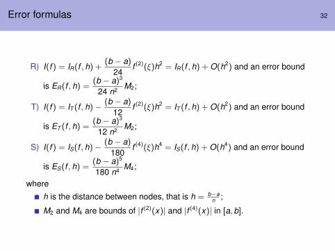
Error formulas 32
R) I(f ) = IR(f , h) +(b − a)
24f (2)(ξ)h2 = IR(f , h) + O(h2) and an error bound
is ER(f , h) =(b − a)3
24 n2 M2;
T) I(f ) = IT (f , h)− (b − a)
12f (2)(ξ)h2 = IT (f , h) + O(h2) and an error bound
is ET (f , h) =(b − a)3
12 n2 M2;
S) I(f ) = IS(f , h)− (b − a)
180f (4)(ξ)h4 = IS(f , h) + O(h4) and an error bound
is ES(f , h) =(b − a)5
180 n4 M4;
where
h is the distance between nodes, that is h = b−an ;
M2 and M4 are bounds of |f (2)(x)| and |f (4)(x)| in [a, b].
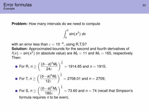
Error formulas 33Example
Problem: How many intervals do we need to compute∫ 2
0sin(x2) dx
with an error less than ε = 10−6, using R,T,S?Solution: Approximated bounds for the second and fourth derivatives off (x) = sin(x2) (in absolute value) are M2 = 11 and M4 = 165, respectively.Then:
For R, n ≥(
(b−a)3M2
24ε
) 12
= 1914.85 and n = 1915;
For T, n ≥(
(b−a)3M2
12ε
) 12
= 2708.01 and n = 2709;
For S, n ≥(
(b−a)5M4
180ε
) 14
= 73.60 and n = 74 (recall that Simpson’s
formula requires n to be even).
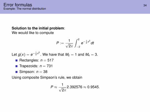
Error formulas 34Example: The normal distribution
Solution to the initial problem:We would like to compute
P :=1√2π
∫ 2
−2e−
12 x2
dt
Let g(x) = e−12 x2
. We have that M2 = 1 and M4 = 3.
Rectangles: n = 517
Trapezoids: n = 731
Simpson: n = 38
Using composite Simpson’s rule, we obtain
P ≈ 1√2π
2.392576 ≈ 0.9545.

Lecture 7 1
Differential equations

Definitions and examples 2
Definitions and examples
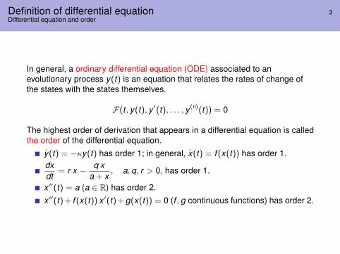
Definition of differential equation 3Differential equation and order
In general, a ordinary differential equation (ODE) associated to anevolutionary process y(t) is an equation that relates the rates of change ofthe states with the states themselves.
F(t , y(t), y ′(t), . . . , y (n)(t)) = 0
The highest order of derivation that appears in a differential equation is calledthe order of the differential equation.
y(t) = −κy(t) has order 1; in general, x(t) = f (x(t)) has order 1.dxdt
= r x − q xa + x
, a, q, r > 0, has order 1.
x ′′(t) = a (a ∈ R) has order 2.
x ′′(t)+ f (x(t)) x ′(t)+g(x(t)) = 0 (f , g continuous functions) has order 2.

Definition of differential equations 4Additional remarks
Sometimes, we avoid writing the independent variable (it is implicitlyassumed to be there and can be deduced from the context):
y = −κy , x = r x − q x/(a + x), x ′′ = a, x ′′ + f (x) x ′ + g(x) = 0,. . .
Note also that the derivative is expressed with different notations:dxdt
= x ′(t) = x(t) = . . .
When the evolutionary process depends on more than one variable, thedifferential equation is called a partial differential equation. For instance
∂2u∂t2 = α
∂2u∂x2 ,
where u = u(t , x) is the temperature at time t on the position x along a1D axis (it is called the heat equation).
We have seen different examples of ordinary differential equations along thecourse that we revisit here in short.
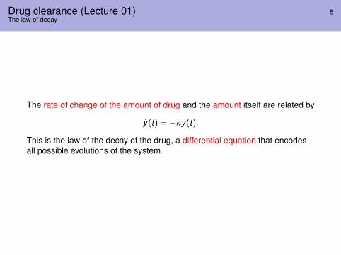
Drug clearance (Lecture 01) 5The law of decay
The rate of change of the amount of drug and the amount itself are related by
y(t) = −κy(t).
This is the law of the decay of the drug, a differential equation that encodesall possible evolutions of the system.

Drug clearance (Project 1, List 01) 6Adding digestive absorption
Assume Ibuprofen is slowly absorbed from the digestive system and relativelyquickly eliminated from the body.Let be:
x , the amount of drug in the digestive system;
y , the amount of drug in the bloodstream.
Notice that, initially, the whole dose A is in the digestive system, thusx(0) = A, y(0) = 0. We get the system of ODEs:{
x(t) = −b x(t),y(t) = −k y(t) + b x(t),
where k is the clearance rate for the bloodstream, and b is the clearance ratefor the digestive system.
x(t) = Ae−bt , y(t) =A b
b − k
(e−k t − e−b t
)
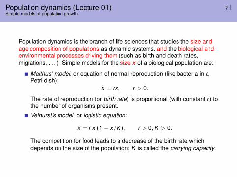
Population dynamics (Lecture 01) 7 ISimple models of population growth
Population dynamics is the branch of life sciences that studies the size andage composition of populations as dynamic systems, and the biological andenvironmental processes driving them (such as birth and death rates,migrations, . . . ). Simple models for the size x of a biological population are:
Malthus’ model, or equation of normal reproduction (like bacteria in aPetri dish):
x = rx , r > 0.
The rate of reproduction (or birth rate) is proportional (with constant r ) tothe number of organisms present.
Velhurst’s model, or logistic equation:
x = r x (1− x/K ), r > 0,K > 0.
The competition for food leads to a decrease of the birth rate whichdepends on the size of the population; K is called the carrying capacity.
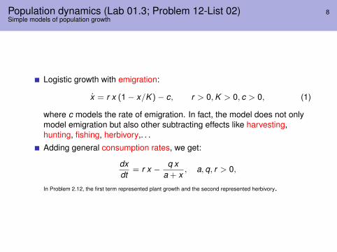
Population dynamics (Lab 01.3; Problem 12-List 02) 8Simple models of population growth
Logistic growth with emigration:
x = r x (1− x/K )− c, r > 0,K > 0, c > 0, (1)
where c models the rate of emigration. In fact, the model does not onlymodel emigration but also other subtracting effects like harvesting,hunting, fishing, herbivory,. . .
Adding general consumption rates, we get:
dxdt
= r x − q xa + x
, a, q, r > 0,
In Problem 2.12, the first term represented plant growth and the second represented herbivory.

Solving differential equations 9Quantitative and qualitative methods
Solving differential equations: quantitative and qualitativemethods

Drug clearance 10The initial value problem
The evolution of the system is (presumably) determined by the initialcondition, say y(0) = A. We have then to solve an initial value problem1:
y(t) = −κy(t), y(0) = A.
Notice that y(t) > 0, so that we can divide by y(t) to get
−κ =y(t)y(t)
=ddt
(log y(t)).
Integrating from time 0 to t both sides of the equation, we get:
−κt =∫ t
0
ddt
(log y(t)) dt = [log y(t)]t0 = log y(t)− log A = log(
y(t)A
),
where we have used the fundamental theorem of calculus, aka Barrow’s rule.Finally, we get the expected evolution
y(t) = e−κtA.
1General solution, particular solution.

Modeling drug clearance 11Solving a simple differential equation
Remarks:
Observe that we need to integrate to solve a differential equations. Inparticular ODEs of type y ′(x) = f (x) are equivalent to solving
∫f (x) dx .
Differential equation/initial value problem are related, respectively, toindefinite/definite integral;
Most of the differential equations can not be solved by hand, and onecan use numerical methods (also known as integration methods, as inLecture 06), whose theoretical basis are, generally, Taylor expansion andinterpolation.
Global features of the systems can be studied by using qualitative ratherthan quantitative approach. In the present example:
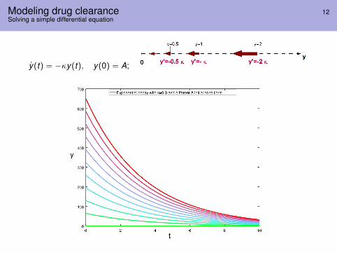
Modeling drug clearance 12Solving a simple differential equation
y(t) = −κy(t), y(0) = A;

Population dynamics 13Qualitative analysis and bifurcation analysis for the logistic growth with (constant) emigration
x = r x (1− x/K )− c =: f (x ; r ,K , c), r > 0,K > 0, c > 0.
We study the sign of x . Accordingly, we solve
f (x ; r ,K , c) = 0⇒ x (1− x/K ) = c/r ,
which are called equilibria.
Obs.: f = 0 at x = 0,K , f > 0 iff x ∈ (0,K ), f ′ = 0 at x = K/2, f (K/2) = K/4and f ′(0; r ,K , c) = r .

Population dynamics 14Qualitative analysis and bifurcation analysis for the logistic growth with (constant) emigration
x = r x (1− x/K )− c =: f (x ; r ,K , c), r > 0,K > 0, c > 0.
f = 0 at x = 0,K ; f > 0 iff x ∈ (0,K ); f ′ = 0 at x = K/2, f (K/2) = K/4;f ′(0; r ,K , c) = r .
The equation can have 0, 1 or 2 equilibria. There is a (saddle-node)bifurcation when c = (r K )/4 (computations on the blackboard).
When c < (r K )/4, x∗± :=K2 r
(r ±
√r 2 − 4 c r/K
)are the equilibria;
x∗− unstable and x∗+ is stable (hint: look at the sign of f (x).)
When c = (r K )/4, x∗ := x∗− = x∗+ =K2
is the unique equilibrium and issemistable.

Population dynamics 15Qualitative analysis and bifurcation analysis for the logistic growth with (constant) emigration.
Remark: Bifurcation analysis let us study the different possible behaviours ofa system with respect to certain control parameters (like r ,K , c), so we cantune them appropriately to get a desired effect.
Exercise: Prove that f ′(x∗−) > 0 and f ′(x∗+) < 0 when c < (r K )/4, andf ′(x∗) = 0, f ′′(x∗) < 0 when c = (r K )/4. Observe that, in general, the signof f ′ at the equilibrium points determines their stability character. Find andclassify the equilibrium points of x = f (x) when f (x) = x2 and f (x) = x3.

A model for Spruce Budworm 16
Spruce budworm (Choristoneura fumiferana) damage appears in May.Evidence of a spruce budworm infestation includes the destruction of buds,abnormal spreading of new twigs, defoliation of current-year shoots and, if anaffected branch is disturbed, the presence of large numbers of larvaesuspended from strands of silk.
Pest damage: Examples of LIGHT, MODERATE andSEVERE mortality of lodgepole pine. See also
http://www.ncrs.fs.fed.us/gla/natdist/mn_sbw.htm

A model for Spruce Budworm 17Qualitative analysis and bifurcation analysis for the logistic growth with general rate of consumption
x = r x (1− x/K )− x2
1 + x2 , r > 0,K > 0, q > 0.
x = 0 is always an unstable equilibrium.Depending on the parameter values, we can have 0, 1 or 2 moreequilibria. All is reduced to study the intersections between functionsg(x) := r (1− x/K ) and h(x) := x/(1 + x2) (see figures below and computations on
the blackboard).
Intersections giving equilibria and2-parameter bifurcation diagram (q = K
in our example).

Neuronal dynamics 18How to model action potentials
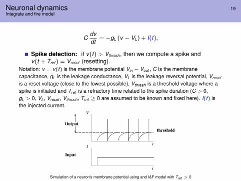
Neuronal dynamics 19Integrate and fire model
Cdvdt
= −gL (v − VL) + I(t),
Spike detection: if v(t) > Vthresh, then we compute a spike andv(t + Tref ) = Vreset (resetting).
Notation: v = v(t) is the membrane potential Vin − Vout , C is the membranecapacitance, gL is the leakage conductance, VL is the leakage reversal potential, Vreset
is a reset voltage (close to the lowest possible), Vthresh is a threshold voltage where aspike is initiated and Tref is a refractory time related to the spike duration (C > 0,gL > 0, VL, Vreset , Vthresh, Tref ≥ 0 are assumed to be known and fixed here). I(t) isthe injected current.
Simulation of a neuron’s membrane potential using and I&F model with Tref > 0

Neuronal dynamics 20Integrate and fire model
The equation
Cdvdt
= −gL (v − VL) + I(t),
is a linear differential equation. We will solve it both quantitatively (LDE canbe always solved) and qualitatively. We take C = 1 for simplicity).
Case I(t) = I constant:v = VL + I/gL is a stable fixed point. Then, we will have spikes if andonly if Vthresh < VL + I/gL.
For I = 0, v(t) = VL + (v0 − VL) exp(−gL (t − t0)), assuming v(t0) = v0
(initial value problem). Hint: use z(t) := v(t)− VL. Observe that
limt→+∞
v(t) = VL.
For I 6= 0, we assume z(t) = C(t) exp(−gL(t − t0)) and we get (aftercomputations):
v(t)−VL = I/gL+(v0−VL−I/g) exp(−gL (t−t0)); thus, limt→+∞
v(t) = VL+I/gL.
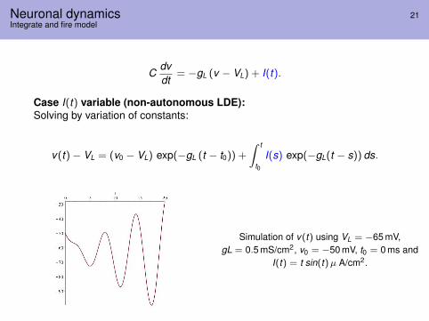
Neuronal dynamics 21Integrate and fire model
Cdvdt
= −gL (v − VL) + I(t).
Case I(t) variable (non-autonomous LDE):Solving by variation of constants:
v(t)− VL = (v0 − VL) exp(−gL (t − t0)) +∫ t
t0
I(s) exp(−gL(t − s)) ds.
Simulation of v(t) using VL = −65 mV,gL = 0.5 mS/cm2, v0 = −50 mV, t0 = 0 ms and
I(t) = t sin(t)µ A/cm2.