Embed Size (px)
Citation preview

1
CALCULUS AS GEOMETRY
FRANK ARNTZENIUS AND CIAN DORR
Near-‐final draft. Forthcoming as chapter 8 of Frank Arntzenius, Space, Time and Stuff (Oxford University Press).
• • •
Geometry is the only science that it hath pleased God to bestow on mankind.
Thomas Hobbes Mathematicians are like Frenchmen: whatever you say to them they translate into their own language and forthwith it is something entirely different.
Johann Wolfgang von Goethe
8.1 Introduction
Modern science is replete with mathematics. The idea that an understanding of mathematics is an essential prerequisite to understanding the physical world is expressed in a famous quote from Galileo:
Philosophy is written in that great book which ever lies before our eyes — I mean the universe — but we cannot understand it if we do not first learn the language and grasp the symbols, in which it is written. This book is written in the language of mathematics…. (Galilei 1623, p. 197).
And the centrality of mathematics to physics has increased immeasurably since Galileo’s time, thanks in large part to two mathematical innovations of the 17th Century: the invention of analytic geometry (principally due to Descartes and Fermat) and the invention of the calculus (principally due to Newton and Leibniz). First let’s consider analytic geometry. We nowadays are used to the idea that geometrical figures correspond to numerical functions and algebraic equations. But this is not how geometry was done before the 17th Century. Euclid never represented geometrical figures by numerical functions; he talked of straight lines, triangles, conic sections, etc. without ever mentioning any corresponding numerical (coordinate) functions characterising these shapes. It is true that prior to the 17th Century on occasion real numbers were used in order to represent geometrical figures, but there

2
was no systematic use of algebraic equations to represent and solve geometrical problems until the early 17th Century. It was Descartes and Fermat who first established a systematic connection between geometrical objects on the one hand and functions and algebraic equations on the other hand by putting ‘Cartesian’ coordinates on space, and then using the numerical coordinate values of the locations occupied by the geometrical objects to characterize their shapes. This made a vast supply of new results and techniques available in geometry, physics and science more generally. Now let’s turn to the calculus. We are also used to the idea that whenever one has a quantity which varies (smoothly) in time, one can ask what its instantaneous rate of change is at any given time. More generally when one has a quantity which varies (smoothly) along some continuous dimension, we nowadays immediately assume the existence of another quantity which equals the rate of change of the first quantity at any given point along the dimension in question. However, until Galileo started to make use of instantaneous velocities in the early 17th Century, instantaneous rates of change had almost no use in science. Even Galileo himself had no general theory of instantaneous velocities, had no general method for calculating instantaneous velocities given a position development, and at times made incoherent assertions about instantaneous velocities.1 It took Newton and Leibniz to develop a general theory of instantaneous rates of change, and to develop an algorithm for calculating their values. This theory was the calculus. And of course most of physics, indeed much of modern science, could not possibly have developed without the calculus.
There are two ways in which this incursion of mathematics into physics is worrying. The first worry involves the relations that physical objects bear to mathematical entities like numbers, functions, groups, and so forth. Much of the vocabulary used in standard physical theories expresses such relations: for example, ‘the mass in grams of body b is real number r’; ‘the ratio between the mass of b1 and that of b2 is r’; ‘the strength of the gravitational potential field at point p is r’; ‘the acceleration vector of body b at time t is v’. Some of these “mixed” mathematico-‐physical predicates have standard definitions in terms of others; but in general, some such predicates are left undefined. But there would be something unsatisfactory about this, even if we were completely comfortable with the idea that entities like real numbers are every bit as real as ordinary physical objects. We would like to think that the physical world has a rich intrinsic structure that has nothing to do with its relations to the mathematical realm, and that facts about this intrinsic structure explain the holding of the mixed relations between concrete and mathematical entities. The point
1For instance, he gave a fallacious argument that it was impossible for instantaneous velocities to be proportional to distance traversed.

3
of talking about real numbers and so forth is surely to be able to represent the facts about the intrinsic structure of the concrete world in a tractable form. But physics books say hardly anything about what the relevant intrinsic structure is, and how it determines the mixed relations that figure in the theories. So there is a job here that philosophers need to tackle, if they want to sustain the idea that the truth about the physical world is determined by its intrinsic structure.
The second worry has to do with the very existence of mathematical entities—numbers, sets of ordered pairs, Abelian groups, homological dimensions of modular rings, and so on. These things are not part of the physical universe around us. They do not interact with physical objects, or at least, they do not do so in anything like the way in which physical objects interact with one another. Some, including us, consequently cannot shake the suspicion that mathematical objects do not really exist.2 But if they don’t exist, shouldn’t it be possible, at least in principle, to characterise the physical world without talking about them at all? Here is another job for philosophers: to find alternatives to standard ‘platonistic’ (mathematical-‐entity-‐invoking) physical theories which can do the same empirical explanatory work without requiring any mathematical entities to exist.
We will call the project of responding to the first worry, by showing how all the ‘mixed’ vocabulary of some platonistic physical theory can be eliminated in favour of ‘pure’ predicates all of whose arguments are concrete physical entities, the ‘easy nominalistic project’. To the extent that we are moved by the second worry, we will want not only to find such predicates, but to write down some simple laws stated in terms of them which presuppose nothing about the existence of mathematical entities. Call this the ‘hard nominalistic project’.
There is an influential line of thought (propounded by Putnam (1971) amongst others) that has convinced many philosophers that the first worry, about the very existence of mathematical entities, is misplaced. The idea is that just as the success of theories which entail that there are electrons (for example) gives us good reason to believe that electrons do in fact exist, so the success of theories which entail that there are real numbers gives us the same kind of reason to believe that real numbers do in fact exist.
One concern about this thought is the fact that, whereas we ended up with electron-‐positing theories as a result of a rather thorough exercise in which these theories were compared with a wide range of rivals which didn’t posit electrons, and the latter theories were found wanting, scientists have generally invested no effort in
2 See Dorr 2007 (section 1) for some attempts to clarify the meaning of this claim.

4
even developing alternatives to standard theories that don’t posit the same range of mathematical entities, let alone in comparing their merits. Instead, practicing scientists simply take it for granted that they can to help themselves to as many mathematical entities as they like—their attitude in this case is utterly different to their attitude towards the positing of physical entities. Because of this, it looks rash to take the fact that all of our currently most empirically successful theories presuppose the existence of certain mathematical entities as a good reason to assume that there are no other, equally successful theories that avoid such presuppositions. Since scientists don’t seem interested, the task of looking for such theories and comparing them with the usual ones—the hard nominalistic project—falls on philosophers.3
There are prima facie reasons to be optimistic about this undertaking. For very often, standard mathematical physics invokes mathematical entities that have “surplus structure” relative to the physical phenomena. For example, when we ‘put’ a coordinate t on, say, time, we are assuming the existence of a function from a very rich structure, namely the real line, onto a much less rich structure, namely time. The rich structure of the real number line includes both an ‘addition structure’ and a ‘multiplication structure’: there are facts about which real number you get when you add two real numbers, and which real number you get when you multiply two real numbers. Time does not have any such structure: it does not make sense to ask which location in time you get when you ‘add’ two locations in time, or ‘multiply’ two locations in time. Or to be more precise: we could introduce meanings for ‘add’ and ‘multiply’ on which this would make sense; but in order to do this, we would have to make some arbitrary choices which are not in any sense dictated by the nature of the entities we are dealing with, namely times. (For example, assuming the falsity of the view discussed in chapter 1 according to which time lacks metric structure we could institute such meanings by choosing one instant of time, arbitrarily, to call ‘zero’, and another to call ‘one’.) The disparity between the two structures shows up in the fact that there are many different coordinate functions that are equally “good”, equally well adapted to the task of representing the kind of structure that time really does have. It is natural to suspect that this detour through an unnecessarily rich structure can be cut out. There has to be 3 Dorr (2010) argues that the it is not so hard to find such laws, since given any platonistic theory T, the theory that T follows from the truth about the concrete world together with certain mathematical axioms can provide satisfactory explanations of the phenomena putatively explained by T, without committing us to the actual existence of mathematical entities. However, the task of evaluating such ‘parasitic’ theories raises tricky epistemological issues. In this chapter, we will be looking for theories which avoid talking about mathematical entities altogether, even in the scope of modal operators. If we can find them, our response to the ‘indispensability argument’ for the existence of mathematical entities will be on firmer epistemological ground.

5
some way of characterising time intrinsically, other than by saying which coordinate functions on it count as “good”; and once we have settled on a systematic way of doing this, it seems plausible that we would then have a way to say what needs to be said without dragging real numbers into the picture at all.
Even if the hard nominalistic project went as well as we could possibly hope—even if we found some general algorithm for systematically turning any scientific theory into an equally simple, empirically equivalent theory free from all presuppositions about the existence of mathematical entities—some philosophers would remain unmoved. There are some who think it is just obvious that mathematical entities do exist, independent of any detailed results from empirical science. Some say: look, real scientists seem to treat it as obvious that these things exist, since they constantly presuppose their existence in theorising about other subject matters, and take no interest (at least, no professional interest) in the project of coming up with theories which do not make require such a presupposition; if this attitude is good enough for them, it should be good enough for us. We will not try to argue anyone out of attitudes like this. But we will just note a couple of things. First, if it turns out that the kinds of empirical considerations that might support belief in electrons do not similarly support the belief that there are mathematical entities, that would be an interesting epistemological discovery even if it in fact the latter belief is well-‐justified for some other reasons. Second, your understanding of platonistic physical theories will be deeper if you understand when quantification over mathematical entities is merely playing an expressive role that could equally well have been achieved in some other way, and when—if ever—it is really essential. And third, even if you think it is completely absurd to suppose that mathematical entities don’t exist, you could and should be interested in the easy nominalistic project, of finding some pure predicates which characterise the intrinsic structure of the physical world upon which the relations between physical and mathematical entities supervene. And once you have gone this far, you should care about finding physical laws that are simple when expressed in terms of your chosen primitive predicates. Even if you don’t mind quantifying over mathematical entities, this could turn out to be a highly non-‐trivial task, and might require overcoming many of the same challenges posed by the hard nominalistic project. For example, you will want to find simple geometric axioms which entail that the intrinsic structure of space is such as to allow coordinates to be assigned in a way that respects that structure.
Historically, those who have worried about the existence of numbers, sets and so forth have often also worried about the existence of regions of space, time or spacetime. Other chapters of this book have argued that we really do have good empirical reason to

6
believe in these entities. Theories that posit them are genuinely simpler, and for that reason more credible, than theories that don’t. So in searching for ways of doing physics without quantifying over real numbers, sets, functions, etc., we will want to pay special attention to the work that geometric entities can do in providing substitutes for such quantification. It is instructive in this regard to see that two of the fathers of the mathematisation of physics, Galileo and Newton, favoured the ‘geometrisation’ of physics, not the ‘arithmetisation’ of physics. To see that this is what Galileo thought, let us extend that famous quote from Galileo a little beyond the place that it is usually ended. Here is how it continues:
… This book is written in the language of mathematics, and the symbols are triangles, circles and other geometrical figures, without whose help it is impossible to comprehend a single word of it; without which one wanders in vain through a dark labyrinth.
Galileo’s ‘language of mathematics’ seems to be the language of geometry, not of arithmetic or algebra. Newton, in turn, was extremely critical of Descartes’ analytic geometry, in which geometry and algebra are joined together:
To be sure, their [the ancients’] method is more elegant by far than the Cartesian one. For he [Descartes] achieved the result by an algebraic calculus which, when transposed into words would prove to be so tedious and entangled as to provoke nausea, nor might it be understood. (Newton 1674−84, p. 317).
Henry Pemberton, who knew Newton well, had this to say:
I have often heared him [Newton] censure the handling of geometrical subjects by algebraic calculations…… and speak with regret of his mistake at the beginning of his mathematical studies, in applying himself to the works of Des Cartes and other algebraic writers before he had considered the elements of Euclide with that attention which so excellent a writer deserves. (Pemberton 1728)
Newton eventually came to the opinion that the proper way to do calculus was as a geometric theory, by means of his ‘synthetic method of fluxions’, and was critical of his own earlier ‘analytic method of fluxions’ which relied on algebraic classifications of curves and numerical power series:

7
Men of recent times, eager to add to the discoveries of the ancients, have united specious arithmetic with geometry. Benefitting from that, progress has been broad and far-‐reaching if your eye is on the profuseness of an output, but the advance is less of a blessing if you look at the complexity of its conclusions. For these computations, progressing by means of arithmetical operations alone, very often express in an intolerably roundabout way quantities which in geometry are designated by the drawing of a single line. (Newton 1674−84, p. 421)
Perhaps the above quotes do not quite amount to a ringing endorsement of a full-‐on attempt to rid physics of all real numbers, sets, functions, groups and the like. Still, we will take ourselves to be encouraged by Newton and Galileo, and set off on that enterprise. We will start by summarising, and slightly amending, the one serious attack on the hard nominalistic project that has been made up to now: Hartry Field’s nominalisation of Newtonian gravitational physics (Field 1980). After that we will attempt to push the project forward, by developing a way of nominalising the theory that lies at the heart of modern calculus and modern physics, namely the theory of differentiable manifolds.
8.2 Nominalizing Newtonian Gravitation.
Field undertakes a case study in the hard nominalistic project. He considers a certain physical theory formulated in the standard way (that is, using lots of mathematical entities), and shows how to write down a completely nominalistic successor for this theory, which can do just as good a job as the original theory at explaining the phenomena. The particular physical theory that Field chooses for this case study is a version of Newtonian gravitation. Of course this theory doesn’t have a hope of being true. For one thing, it says that the only form of interaction is by gravitation, and we know perfectly well that this is not the case. So the nominalistic successor theory doesn’t actually do a good job at explaining all that needs to be explained by a physical theory. But the point of a case study like this is to notice general strategies which we can put to work in finding nominalistic successors for other platonistic physical theories. Ultimately, we would like to consider whole families of theories sharing some general structural features. Then we could formulate general results of the form ‘so long as the phenomena do not require us to reach for mathematical tools beyond those invoked by theories of this class, they can be explained without invoking mathematical entities at all’.

8
One salient feature of the Newtonian theory chosen by Field is its flat spacetime setting—that of so-‐called Neo-‐Newtonian (or “Galilean”) spacetime. (See chapter 1, section 2 for an explanation.) The basis of Field’s nominalistic physics is an axiomatic characterisation of this Neo-‐Newtonian spacetime, which builds on the axiomatic Euclidean geometry developed by Hilbert (1899) and Tarski, and the axiomatic affine geometry developed by Tarski and Szczerba. This axiomatisation uses just three primitive predicates, all of which take spacetime points as arguments: a two-‐place Simultaneity predicate, a three-‐place Betweenness predicate, and a four-‐place ‘spatial congruence’ predicate ‘S-‐Cong’. (‘S-‐Cong(a,b,c,d)’ intuitively means that points a and b are exactly as far apart as points c and d. It is a consequence of the axioms that whenever SCong(a,b,c,d), a and b are Simultaneous and c and d are Simultaneous: this captures the fact that no notion of absolute rest is definable within Neo-‐Newtonian spacetime.) The axioms that Field uses are essentially nothing more than a modern, rigorous, version of the axioms that Euclid set down more than 2000 years ago. For example, one of them is the ‘Axiom of Pasch’: if Between(x,u,z) and Between(y,v,z), then for some a, Between(u,a,y) and Between(v,a,x). Or in words: given a triangle xyz, with a
point u on the side xz and a point v on the side yz, there is a point a where the
xor
c
y
v
z u
aa
Figure 1: The Axiom of Pasch

9
lines uy and vx intersect (see Figure 1.) These axioms do not mention real numbers, functions, sets, or anything like that. Like Newton himself, the theory shuns Descartes and imitates Euclid. We will later on discuss one of the axioms, a ‘richness’ axiom that is quite different in character from the other axioms, in a little bit more detail. But for now, let us push ahead and sketch Field’s treatment of the contents of this space-‐time. The particular mathematical version of Newtonian gravity that Field takes as his input has two parts. First, there is a theory about the relations between two spacetime fields—the mass density field and the gravitational potential. Second, there is a theory about the relations between the second of these fields and the spatiotemporal trajectories of so-‐called ‘test particles’. Let us begin by considering just the first part. In mathematical terms, one would think of both the mass-‐density field and the gravitational potential as functions from spacetime points to real numbers. Relative to any coordinate system, each such function will correspond to a function from quadruples of real numbers to real numbers. The claim the theory makes about the relation between these fields can then be expressed as a condition on the latter functions, namely Poisson’s equation:
∂2φ/∂x2+∂2φ/∂y2+∂2φ/∂z2=−kρ
Here φ(x,y,z,t) is the function from ℝ4 to ℝ that represents the gravitational potential, and ρ(x,y,z,t) is the one that represents the mass-‐density field. k is a constant.
This is a good illustration of the challenges involved in both the easy and the hard nominalistic project. To carry out the easy project, we would have to explain what it is for a given real number to be the value of the gravitational potential or of the mass density field at a spacetime point. Moreover, our explanation should do justice to the fact that there is something arbitrary about the use of real numbers in this connection, insofar as the mapping depends on an arbitrary choice of a unit for mass, and of a unit and a zero for the gravitational potential. To carry out the hard project, we will also have to dispense with the extensive quantification over mathematical entities required by this formulation: as things stand, we are quantifying over functions from spacetime points to real numbers (the coordinate functions), over functions from real numbers to real numbers (the coordinate representatives of the fields), and over functions from some such functions to other such functions (since differentiation is standardly explained as “the” function of this sort satisfying certain properties).

10
Field’s approach is as follows.4 To talk about the gravitational potential we will use two predicates, GravPotBetweenness and GravPotCongruence, subject to one-‐dimensional analogues of the axioms for spatial betweenness and congruence discussed earlier. Just as the geometric axioms entail that a unique mapping from points of space to points of ℝ4 is determined once we settle which points we want to map to <0,0,0,0>, <1,0,0,0>, <0,1,0,0>, <0,0,1,0> and <0,0,0,1>, so the axioms for GravPotBetweenness and GravPotCongruence will let us determine a unique mapping from points of space to ℝ once we decide on a pair of points which we want to map to 0 and 1 respectively. To talk about the mass density field, we can use a single predicate MassDensitySum—where intuitively MassDensitySum(x,y,z) means that the real number that is the value of the mass density field at z is the sum of those that are its values at x and y—subject to axioms which determine a unique mapping to the real numbers once we have chosen a point (with nonzero mass density) to map to the real number 1. (We use MassDensitySum rather MassDensityBetwenness and MassDensityCongruence because there is an objective fact about which points have zero mass-‐density, whereas there is no objective fact as to which points have zero gravitational potential, any more than there is an objective fact about which instant of time is the ‘zero instant’. This also explains why numerical representations of mass-‐density are unique up to transformations of the form m→am, rather than of the form m→am+b.)
Thinking of the gravitational potential as a fundamental field on a par with mass-‐density may seem surprising. Since Poisson’s equation completely determines the facts about the gravitational potential at each time given the facts about the mass-‐density field at that time, it is tempting to regard the gravitational potential as nothing more than a device for summarising certain facts about the distribution of mass-‐density that have a special relevance when we are trying to figure out how things (in Field’s theory, “test particles”) will accelerate at a given point. Someone who was only concerned with the easy nominalistic project could afford to go along with this attitude. But Field is engaged in the hard project: he wants a simple nominalistic theory which can do all of the explanatory work of the platonistic theory it replaces. Taking the gravitational potential to be a fundamental scalar field is a crucial part of Field’s strategy for doing this. Without it, it is completely unclear how one could express in a nominalistically acceptable way a law determining the net force on each particle as a sum of component forces deriving from all the rest of the mass in the universe. We think Field is thinking in the right way here. As has been emphasised many times in this book, the right way to form views about the fundamental structure of the world is to be guided by the idea that
4 Field isn’t quite explicit about the primitive predicates he wants to use in the case of the mass density field; what we describe is one way of doing it.

11
the laws are simple when stated in terms of fundamental predicates. In this way we can be justified in positing fundamental structure that is “nomologically redundant”, in the sense that the facts about part of the structure follow, given the laws, from facts about the rest of the structure. For such redundacy might obtain without there being any simple definition of the redundant predicates in terms of the others.
To state a nominalistic version of Poisson’s equation as given above, the central thing we need to be able to do is to take directional derivatives. For instance we need to give a nominalistic expression which says that the derivative of the gravitational potential φ at spatial point p in direction V equals the derivative of gravitational potential φ at spatial point q in direction W (see Figure 2).
Figure 2: Sameness of directional derivative
How do we say that? Well, in the friendly setting of Euclidean space, a vector V at a point p can be identified with a straight line p→p′ which runs from p to another point p′ (the direction of the line corresponding to the direction of V, and the length of the line corresponding to its magnitude), and a vector W at q can be identified with a straight line q→q′. If φ were to change at a constant rate along the lines p→p′ and q→q′, then directional derivatives of φ at p in direction V and at q in direction W would be equal iff the ratio between the difference in the value of φ between p′ and p and the difference in the value of φ between q′ and q were equal to the ratio between the lengths of p→p′ and q→q′. Of course, generically the potential does not change at a constant rate between a point p and a point p′ which is a finite distance away. So we need to take limits as we get closer and closer to p and q, while keeping the ratio and directions fixed. Here is how to express the claim nearly nominalistically:
For all points w,x,y,z such that φ(w)−φ(x):φ(y)−φ(z) > 1, there exist a point p′′ Between p and p′, and a point q′′ Between q and q′, such that, for any point p′′′ Between p and p′′ and any point q′′′ Between q and q′′: if |q→q′′′|:|p→p′′′|=|q→q′|:|p→p′|, then φ(y)−φ(z):φ(w)−φ(x) < φ(p′′′)−φ(p):φ(q′′′)−φ(q) < φ(w)−φ(x):φ(y)−φ(z).
Here |q→q′′′|:|p→p′′′| is the ratio of the lengths of lines q→q′′′ and p→p′′′. The idea is that the directional derivative of φ at p in direction V equals the directional derivative of φ at q in direction W iff for any desired degree of accuracy one can find a point p′′ in direction V from p, and a point q′′ in direction W from q, such that for any points p′′′ and q′′′ in the same directions from p, such that their distances from p and q respectively
p v p
φ
q'
q Space w

12
stand in the same ratio as V to W, the ratio of the difference between values of φ at p and p′′′ and the difference between values of φ at q and q′′′ is within that degree of accuracy of 1. The ‘degree of accuracy’ demand is imposed by saying that it has to be smaller than φ(w)−φ(x):φ(y)−φ(z) for any such ratio that is larger than 1, and also larger than its inverse.
The above is not yet expressed in terms of the primitive congruence and betweenness predicates: we have not said how to express claims about the inequality and equality of ratios of lengths of lines and of gravitational potential differences. But it is not surprising that this can in fact be done, given the central role such claims play in Euclid’s geometry. (For the details of this, and about how to use these tools to express the more complicated claim about differentiation required to nominalise Poisson’s equation, see Field 1980, chapter 8.) Thus in this case at least, the grounds for optimism we mentioned in section 8.1 are vindicated. The aspects of calculus that are needed to state the physical theory can be developed using just the geometric structure expressed by the relevant betweenness and congruence predicates, without appeal to the richer structure characteristic of the real number line. The claim quoted above may look dauntingly complex, but in fact the result of unpacking the standard definitions of differentiation in terms of limit, and of limit claims in terms of quantification over epsilons and deltas, results in something formally isomorphic.5
So far this is far from being anything like a fully worked out Newtonian gravitational theory. Poisson’s equation determines the gravitational potential given the mass density field, but it does nothing at all to constrain the mass-‐density field. The second part of Field’s theory, which concerns particles, gives us something a bit more like what we would have expected, since it tells us how “test particles” move in response to the gravitational potential. The claim is aversion of Newton’s second law: the acceleration of each particle p is proportional to the gradient of the gravitational potential at the place where it is, divided by the particle’s mass. However, the total package is still manifestly unsatisfactory, in that it says nothing about the relation between the mass-‐density function and the point particles, and indeed still leaves the former entirely unconstrained. There are various ways in which this particular defect could be remedied. For example, we could replace point-‐particles with little spheres of constant mass-‐density, which respond to the gravitational potential as if their masses were concentrated at their centres. Or we could try to get rid of point particles in favour 5 Moreover, since the nominalistic theory lets us avoid all the complexity attendant on the usual constructions of real numbers (e.g. as Dedekind cuts of rationals, themselves construed as sets of ordered pairs of natural numbers…), it seems to us that even setting questions of ontological economy to one side, the nominalistic theory has a substantial advantage in terms of simplicity (when formulated in terms of fundamental predicates).

13
of a fully fledged continuous fluid dynamics. Each of these routes raises some tricky issues. For example, with spherical particles, we would need to specify what happens when there is a collision. (The easiest approach is to allow them to pass through each other; but then we will need to take all the particles that may occupy a given point into account when figuring its mass density.) Meanwhile, known theories of continuum dynamics involve lots of unrealistic singularities and discontinuities. However, none of these problems is particularly germane to the nominalistic project.
If we stipulated that all the test particles are equally massive, nominalising the second part of the theory wouldn’t raise any new technical difficulties. We could just add one new primitive predicate Occupies, relating the particles to the spacetime points in their trajectories. The resources required to express the differential equation governing Occupation are similar to the ones required for stating Poisson’s equation. However, allowing the particles to differ in mass brings in a few more complications, which we will discuss in the next section.
8.3 Richness and the existence of property spaces.
Now let us return to the richness axiom that we briefly mentioned in the discussion of geometry above. For the sake of simplicity, let’s see how this would work if we were only concerned with a one-‐dimensional space like time, instead of four-‐dimensional Neo-‐Newtonian spacetime. We want to say something about the TimeBetweenness and TimeCongruence facts which entails, modulo standard mathematics, that any two functions from instants of time to real numbers which ‘respect’ the TimeBetweenness and TimeCongruence facts in certain specified ways are related by a linear transformation. In order to achieve this, our axioms will have to entail that there are lots of instants of time. For instance, if (bizarrely) there were only three instants of time a, b and c, then there would only be one TimeBetweenness fact, and, generically, no TimeCongruence facts other than trivial ones such as TimeCongruent(a,b,a,b). Requiring a mapping from the three instants of time to real numbers to respect these facts does very little to constrain it, and certainly does not pin it down up to a linear transformation. And all of this holds, mutatis mutandis, for spacetime, mass, mass density and the gravitational potential.
So, in each case, Field assumes a richness axiom. Here is the basic idea of the richness axiom in the case of time:
Between any two distinct instants lies another distinct instant, and for any instant there are two distinct instants that it lies between

14
There are two worries about this axiom as stated. The first is that it is not strong enough to force a representation by the real numbers (as opposed to, say, the rational numbers). The second is that in some cases—for example, those of mass and mass density—the axiom is too strong, since there might not be that many distinct masses or mass densities in the world. Field discusses the first worry at length, but largely ignores the second. Let us discuss each in turn. The above axiom is consistent with a set of temporal congruence and betweenness facts which is representable by the rational numbers. After all, for each pair of rational numbers there is one that lies between them, and each rational number lies between two rationals. But the temporal coordinates that are used in physics are real numbers, not rational numbers. Moreover, ever since Pythagoras it has been known that the ratio between the diagonal of a square and its side is irrational. So it looks like we will need the reals rather than the rationals in order to characterize spatial distances.
Field’s response to this worry involves an important new element, namely quantification over arbitrary regions of spacetime as well as points. Given an ontology of regions, and a primitive predicate ‘Part’ that expresses their structure, one can supplement the above “density” axiom with something like the following axiom of “Dedekind completeness”:
For all temporal regions R1 and R2, if no instantaneous Part of R1 is Between two instantaneous Parts of R2, and no instantaneous Part of R2 is Between two instantaneous Parts of R1, there is an instant a such that whenever b is an instantaneous Part of R1 and c is an instantaneous Part of R2, and a≠b and a≠c, then a is Between b and c.
Here is why, intuitively speaking, this forces one to have the real numbers as coordinates. Suppose one had the rationals as coordinates. Now consider the following regions:
R1: all the instants the square of whose coordinate is smaller than 2 R2: all the instants the square of whose coordinate is greater than 2
Since no instant of either of these regions is between two instants of the other, our axiom of Dedekind completeness entails that there is an instant between R1 and R2. But such an instant cannot consistently be assigned any rational-‐numbered coordinate. Every rational number is either smaller than √2, in which case there other rational

15
numbers are bigger than it and yet still smaller than √2, or larger than √2, in which case other rational numbers are smaller than it and yet larger than √2. So we need the reals. This response works only to the extent that our theory entails that there are regions like R1 and R2. So our theory will need to include some axioms about Parthood which provide for the necessary plenitude of regions. The canonical way of doing this is to adopt “classical mereology”, which can be axiomatised as follows:
M1 (‘Reflexivity’): everything is Part of itself M2 (‘Transitivity’): if x is Part of y and y is Part of z, x is Part of z M3 (‘Antisymmetry’): if x is Part of y and y is Part of x, x=y M4 (‘Weak Supplementation’): If x is Part of y, then either x=y or y has a Part that has no Part in common with x. M5 (‘Universal Composition’): For any condition φ: if something is φ, then there is a “fusion of the φs”—something which has every φ as a Part, and each of whose Parts shares a Part with some φ M6 (‘Atomicity’): everything has a Part with no Parts other than itself
However, even then there is a problem, associated with the talk of ‘conditions’ in M5. The problem is a somewhat technical problem in logic. Since this problem is pretty much orthogonal to the main problem that we are interested in this chapter, namely the problem of doing calculus, and differential geometry in particular, in a nominalistic way, we will be brief, referring you for further details to Cohen 1983, Field 1985b, and Burgess and Rosen 1997.
One way to interpret claims like M5 is to take them as expressed in something like second order logic. Or if one wants to use English, one can use plural quantification: ‘For any things whatsoever, there is something that has each of them as a Part, and each of whose Parts shares a Part with one of them’. Another approach to axioms like M5 construes them as first-‐order schemas. On this approach, M5 is shorthand for the infinite collection of axioms we get by substituting particular expressions for ‘φ’. The question which of these approaches is preferable involves deep issues in the foundations of logic which we cannot adjudicate here. But both approaches require one to be careful about the sense in which one might regard the total package of nominalistic theory as “equivalent” to the platonistic theory upon which it was based.
It would be convenient if we could claim that the platonistic theory is nominalistically conservative with respect to the nominalistic one, in the sense that every consequence of the platonistic theory in which all quantifiers are restricted to spacetime regions is already a consequence of the nominalistic theory. This would give

16
us a nice, simple story about why it is acceptable to use the platonistic theory when making calculations. It would be sufficient for this to be the case if we could prove, from the mathematical axioms, a representation theorem to the effect that every model of the nominalistic axioms can be extended to a model of the platonistic theory (with betweenness and congruence defined in the usual ways). However, if we go for the first order construal of the nominalistic theory, this just isn’t true. Anyone who has internalised the lessons of Gödel’s theorems will readily understand why. Just by being so very strong, the platonistic theory (which, let’s suppose, includes something like first-‐order Zermelo-‐Fränkel set theory) can prove sentences which express the consistency of the nominalistic theory, whereas by Gödel’s second incompleteness theorem, these sentences cannot be proved in the nominalistic theory itself. (Such ‘consistency’ sentences can be expressed perfectly well in geometric terms—for example we can construe ‘proofs’ as certain intricately-‐shaped spacetime regions.)
So, the (first order) platonistic theory entails nominalistically-‐statable sentences which are not consequences of the (first order) nominalistic theory. And indeed some of these consequences are extremely plausible, such as the claim that there are no pieces of paper upon which are ink marks that constitute a proof of a contradiction from the axioms of the nominalistic theory. But so what? The claim we wanted to make on behalf of the nominalistic theory was not that it systematises absolutely everything that it is plausible for us to accept on the subject matter of spacetime and its contents. Rather, the claim was just to the effect that the nominalistic theory does as good a job as the platonistic theory at explaining the experimental data that matter for physics; the point of making this claim was to undercut a certain style of argument for the existence of mathematical entities, to the effect that only by positing them can we adequately explain those data. There are many claims about the physical world that are quite plausible for reasons that have nothing to do with experiments. Someone might argue that we should believe in the existence of an enormous hierarchy of sets on the grounds that this satisfyingly explains these kinds of truths. This strikes us as an odd sort of reason for believing in mathematical entities. In any case, it is very different in character from the one which the nominalisation project is designed to undercut.
If we accept the second-‐order or plural version of the nominalistic theory, and think that we understand a notion of “semantic consequence” that floats free from derivability in any formal system, then we are free to accept the claim of nominalistic conservativeness, understood as the claim that every semantic consequence of the platonistic theory with appropriately restricted quantifiers is a semantic consequence of the nominalistic theory. On this approach, the platonistic theory really can be thought of as nothing more than a useful computational device for systematising the

17
semantic consequences of the nominalistic theory—not all of them, but a larger subset than can be derived by applying any ordinary second-‐order proof theory directly to the nominalistic axioms. The question whether this notion of semantic consequence can be understood without commitment to mathematical entities raises deep foundational questions which we will not attempt to engage with here.
An aspect of a second order nominalistic theory that we find more worrying is the following. Once one has a second order theory of regions, one can state claims in one’s language which in effect mean the same thing as claims such as the continuum hypothesis (i.e. the hypothesis that there is no cardinality in between that of the integers and that of the real numbers). Claims like this are puzzling, in part because it is hard to see how one could get evidence for or against their truth. Many have thought it an attractive feature of nominalism that it lets us avoid positing unknowable facts of the matter about questions such as this. But this alleged advantage is not one that can be retained if we embrace a second-‐order theory. (One response to the worry holds that although second order language is intelligible, it is vague enough that claims such as the continuum hypothesis do not get a determinate truth value. But if one takes this view, it is not clear that one can legitimately claim the advantages of simplicity for a theory expressed in such vague terms.)
We will not take a stand about which of the two approaches is the better. None of the problems strike us as devastating. And even if one did think they were devastating, there would still be many reasons to be interested in the details of the nominalisation project, insofar as it is illuminating to understand when talk about mathematical entities is merely giving us a way of saying something we could equally well have expressed “intrinsically”, and when it is really essential to the claim being made.
So let’s set this first worry aside and turn to the second worry, to the effect that that even the “density” axiom might be too strong to be plausibly true of the physical world. Let’s consider the case of mass qua property of point-‐particles. Suppose, e.g. that there are only finitely many point particles in the world, or at any rate only finitely many equivalence classes under the ‘same mass’ relation. Then richness axioms about mass will plainly be false. Indeed, unless the facts about mass are especially well-‐behaved, there will not be anywhere near enough MassSum facts to fix numerical mass values that are unique up to scale transformations. (Note that if the particles are spatially extended and arbitrarily divisible, then there is no such problem: assuming that the mass of a particle is continuously distributed over its parts, any extended particle will then have a continuum of parts with a continuum of distinct mass properties, which will suffice to determine mass values that are unique up to scale transformations.) The same problem may arise if we take mass density as a

18
fundamental quantity. Certainly the laws we have stated do not rule out the hypothesis that the mass-‐density field is discontinuous, in such a way that the world can be divided into finitely many regions each of which is of uniform mass density. And it is not completely physically unrealistic to imagine that the world works like that, at least with respect to some fundamental quantities. What should we do, if we want our strategy for nominalisation not to break down in such cases? One attitude would be to say: so what?—if that is so, then numerical attributions of mass are in fact much more conventional than we took them to be. This, however, seems to us to be the wrong attitude. After all, we can get good evidence that mass values are not conventional (other than up to re-‐scalings), for we can empirically confirm that the amount of acceleration that a particle undergoes, when it is subject to a non-‐gravitational force, is proportional to its mass. That is to say, we can read mass values, up to a re-‐scaling factor, off from the accelerations that objects undergo when subject to certain forces. (Of course this requires certain assumptions about the magnitudes of forces in certain circumstances, but we can have well-‐confirmed simple laws regarding this.)
Now, the fact that we can read mass values off accelerations also suggests a remedy to our problem. For one might suggest that mass is not a fundamental quantity, but rather implictly defined by Newton’s second law: the mass of particle p at t equals the ratio of the gradient of the potential at the point occupied by p at t to the acceleration of p at t. If the only mass-‐facts we were concerned with were facts about the mass of Fieldian ‘test particles’, this would be fine. We could state the laws governing such particles’ trajectories as follows: (i) For any particle and any time, the particle’s acceleration vector points in the same direction as the gradient of the gravitational potential; (ii) For any particle and any two times t1 and t2 at which its acceleration vector and the gradient of the potential are not both zero, the ratio of the magnitudes of these two vectors at t1 is the same at their ratio at t2. We know how to say this sort of thing nominalistically. If we wanted to allow the particles to serve as sources of gravity, by generating curvature in the gravitational potential, we can adapt a similar idea: we would then need a law to the effect that for any two particles p and q, the ratio between the ‘inertial mass ratio’ of p and that of q equals the ratio between the curvature of the gravitational potential around p to that around q.6
However, this programme crucially depends on the fact that the quantity we are interested in (mass) is intimately associated, given the laws, with another quantity
6 Ernst Mach (1893) famously argued that mass is implicitly defined by means of its role in the laws. However, since Mach was equally eager to eliminate the gravitational potential in this way, his project leads to difficulties similar to those we discuss in the next paragraph.

19
(gravitational potential) which, being continuous, is well-‐behaved from the point of richness axioms. In other theoretical settings, no such fall-‐back quantities are available. For instance, we could consider a theory of extended particles of varying mass, which move inertially except for elastic collisions. If we didn’t want to take any facts about the masses of the particles as fundamental, it is very hard to see how we could define them in terms of the other fundamental facts, namely the facts about the shapes of the particles’ trajectories. Well: what we can do is to say that the “mass function” is the unique function from particles to numbers such that product of it with velocity (“momentum”) and the product of it with velocity squared (“kinetic energy”) are both conserved. If collisions are common enough, this may pin down a unique function (up to a linear scaling). But this definition is not at all helpful to us if we are looking for laws that are simple when stated in terms of the fundamental predicates. For it is totally unclear what we could say about the particles that would entail that there is any function that plays the “mass” role just described. And it seems obviously unsatisfactory merely to stipulate that there is such a function, not on nominalistic grounds—probably we could code up such function talk somehow as talk about spacetime regions—but because, as has already been remarked on several occasions in this book, this sort of brute existential quantification is not the sort of thing that could be regarded as an explanatorily satisfactory or plausible fundamental theory.7
There is another strategy for dealing with this problem, which is less dependent on the details of the physical theory in question. One can assume the existence of a ‘mass space’, whose structure is given by MassSum relations, subject to the usual axioms, holding between points in mass space. Each particle is then assumed to ‘Occupy’ a single point in mass space. Note that there can be many points in mass space which are not occupied by anything. One can therefore safely assume that a richness axiom is satisfied, since all that this means is that mass space has points—whether occupied or unoccupied—corresponding to a continuum of distinct mass values. And then it will follow that the mass values of all particles (and all their parts) are determined up to re-‐scalings, no matter how many or how few points in mass space are occupied by particles.8 7 See Dorr 2010 for some tentative attempts to say something general about this kind of explanatory badness. 8 The worry about richness can be dealt with in another way, by using the richness of physical space as a surrogate for the richness of the space of possible masses. One could have a primitive predicate such as this: ‘the ratio between the mass of particle x and particle y equals the ratio between the distance between points a and b and the distance between points c and d’. See Burgess and Rosen 1997 (section II.A.3.c) for more discussion of this kind of approach, which can arise as part of a systematic recipe for nominalising a theory by replacing each variable ranging over real numbers with a quartet of variables ranging over points.

20
Instead of calling the points of mass space ‘points of mass space’ and saying that particles ‘occupy’ them, one could call them ‘mass properties’ and say that particles ‘have’ them. We take it that nothing substantive turns on this choice of terminology. Calling them ‘properties’ might seem to make the positing of them less controversial. There are some views in metaphysics according to which we are obliged to posit a realm of properties as part of our fundamental ontology in any case, no matter how physics turns out. If one subscribed to such a view, one might see a big difference between thinking of some entities as points in an unfamiliar new kind of ‘space’, on the one hand, and thinking of them as belonging to the familiar category of properties, on the other hand. But this is not our attitude. As we have tried to make clear by talking (most of the time) about ‘predicates’ rather than ‘properties’, we think it is an open question, to be settled on physical grounds, whether we should posit any entities that could by any stretch of the imagination deserve the label ‘properties’. And as we will see, it is quite helpful to think of entities like the ones we are currently contemplating as points in spaces with the same kind of geometrical structure as more familiar spaces.
In fact, the positing of ordinary space or space-‐time is essentially the same sort of move as the positing of mass space: the structure of position properties of particles is (arguably, as we have seen in chapter 5) best given by assuming the existence of a structured space-‐time, and then assuming that each particle occupies a particular region in this structured space-‐time. So why not similarly assume the existence of mass space, when its structure can so simply and nicely explain the usefulness, and the scale arbitrariness, of the canonical numerical representation of the mass properties of objects, and can do so however few distinct mass properties are had by all existing objects? It seems to us that such a posit might not be so hard to justify on the grounds of the theoretical simplicity it yields.
8.4 Differentiable manifolds
Field’s case study is a success so far as it goes. But we would like to be able to nominalise more recent physics. In particular, we would like to be able to have a nominalistic way of stating differential equations governing fields and particles in curved space-‐times and vector bundles, since that is how much of modern physics is done. Key to this is the notion of a differentiable manifold. When one does general relativity, one starts with a differentiable manifold. One can then endow it with metric and affine structure, by means of a metric tensor field (and a compatible connection and volume form); and one can endow it with other kinds of physical properties, in the form of scalar, vector, and tensor fields. When one develops gauge theories, one starts with two differentiable manifolds, namely the space-‐time manifold and the fibre manifold

21
(which are connected via a projection map), and one posits physically interesting structure in the form of sections of the fibre bundle, a connection on the fibre bundle, etc. Moreover, differentiable manifolds are the minimal structure that one needs in order to do calculus. That is to say, given just a differentiable manifold (without a metric), there are facts as to which curves in the manifold are differentiable, which are n-‐times differentiable, which are smooth; there are facts as to which scalar functions on the manifold are differentiable, n-‐times differentiable, smooth; one can define vectors and vector fields; one can define directional derivatives of scalar functions; one can define differential forms; and so on. With anything less than a differentiable manifold one could not do any of this, one would just have a space with a topology, which, from the point of view of calculus, is useless.
How is a differentiable manifold normally defined? Well, one starts with a topological space M, the ‘manifold’. One then divides M up into overlapping open patches (regions) P, and provides each patch P with n coordinate functions, i.e. for each patch P one provides a continuous, one-‐to-‐one map from P to a patch of ℝn (the space of n-‐tuples of real numbers, with its standard topology). Using these coordinates, various calculus-‐related notions that can be defined on ℝn get carried back to M. For this procedure to make sense, we need to guarantee that the notions in question behave in a consistent way when the patches overlap. This is achieved by requiring that when patches P1 and P2 overlap, then on the overlap, each of the coordinates provided for P1 must be a C∞ function of the coordinates provided for P2: that is, for any finite integer m, the coordinates provided for P1 must be m times differentiable with respect to the coordinates provided for P2.
Given this condition, we can consistently make definitions such as the following. A function f from the M to ℝ is smooth iff for each coordinate patch, the induced function from ℝn to ℝ is smooth(C∞). Likewise, a parameterised curve in M—a function from ℝ to M—is smooth iff for any coordinate patch, each of the real number coordinates of the curve is a C∞ function from ℝ to ℝ.
A vector vp at a point p∈M is a map from smooth functions on M to real numbers, such that
(a) vp(f+g)=vp(f) + vp(g), (b) vp(αf)=αvp(f) (c) vp(fg)=f(p)vp(g) + vp(f)g(p).
(See section 2.5 above for why such a map, intuitively speaking, corresponds to a vector at a point.) A covector at a point p is a linear map from vectors at p to real numbers.

22
And a tensor of rank j, k at p is a map that takes j covectors at p and k vectors at p to a real number, and is linear in each of its arguments.
We can define a smooth vector field as a function v that maps each point p to a vector at p, in such a way that whenever f is a smooth function, the function whose value at each point p is v(p)(f) is itself smooth. Alternatively, we can simply identify smooth vector fields with the functions from smooth functions to smooth functions which they induce in this way. On this approach, we define a smooth vector field as a function v from smooth functions to smooth functions such that (a) v(f+g)=v(f) + v(g) (b) v(αf)=αv(f) (c) v(fg)=fv(g) + v(f)g
Similarly, a smooth covector field can be defined as a ‘C∞-‐linear map’ from smooth vector fields to smooth functions, that is, a function ω such that (a) ω(v1+v2) = ω(v1)+ω(v2) (b) ω(fv) = fω(v)9
And a smooth tensor field of rank j, k can be defined as a function that takes j smooth covector fields and k smooth vector fields to a smooth function, and is C∞-‐linear in each of its argument. (Alternatively, as with smooth vector fields, we could treat smooth covector and tensor fields “pointwise”, as functions assigning points to covectors or tensors at those points.)
Note that by this definition covector fields are just tensor fields of rank 0,1. Also, there is a natural correspondence between vector fields and tensor fields of rank 1,0, given in one direction by tv(ω) = ω(v), and in the other by vt(f)=t(df), where df is the covector field defined by df(v)=v(f). So vector fields too can be regarded as a special case of tensor fields.
In the above we used a single specific set of coordinates for certain specific patches P. Of course this seems unnecessarily specific, since any set of patches together with coordinate systems which are everywhere smooth with respect to the specific set in question would have resulted in the same characterisation of differentiability and smoothness, the same vector fields, etc. Therefore often textbooks characterize a differentiable manifold not by a unique coordinate system for a unique set of patches,
9 Here v1+v2 is the vector field defined by (v1+v2)(f) = v1(f)+v2(f), and fv is defined by (fv)(g) = fv(g).

23
but by a maximal equivalence class of coordinate systems and patches which all result in the same characterisation of differentiability etc. These ways of defining differentiable manifolds are not merely awash in real numbers, functions, sets, sets of sets, etc.; they is also spectacularly unsatisfying from a foundational point of view. The fact that a given function from a region of physical spacetime to ℝn is admissible as a coordinate system surely must have some explanation in terms of the region’s intrinsic structure; but the standard approach gives us no clue about what the relevant intrinsic structure might be like. And surely that intrinsic structure is something that could be described independently of any division of the manifold into patches. There is another way of defining differentiable manifolds that is a bit less hamfisted. While it too is replete with mathematical objects, it is more suggestive of directions for the nominalistic project. In this alternative approach, a differentiable manifold is defined as a set of points M together with a distinguished set of functions from those points to the real numbers, which we call the “smooth” functions. These functions are required to obey certain characteristic axioms. Here is one version of the axioms (for an n-‐dimensional manifold), from Penrose and Rindler 1984, section 4.1; similar axiomatisations appear in Chevalley 1946, Nomizu 1956 and Sikorski 1972:
F1 If f1, …, fm are smooth functions on M, and h is any C∞ function from ℝm to ℝ,
then the function from M to ℝ whose value for any point p is h(f1(p), …, fm(p)) is smooth.
F2 If g is a function from M to ℝ, such that for each p∈M there is an open set O containing p, and a smooth function f which agrees with g in O, then g is smooth.
F3 For every p∈M, there is an open set O containing p, and n smooth functions x1, … , xn, such that (i) given any two points in O, at least one of the functions has a different value at the two points, and (ii) for each smooth function f, there is a C∞ function h from ℝn to ℝ, such that f(p) = h(x1(p), …, xn(p)) for all p in O.
Here there is no need to take the notion of an “open set” in M as a further primitive: we can define S to be ‘open’ iff for some smooth h, S = {x: h(x)≠0}.10 10 Given the standard topological definition of a ‘continuous’ function as one such that the inverse image of any open set is itself open, it follows from this that all smooth functions are continuous. For any open O⊂ℝ, we can find a C∞ function hO:ℝ→ℝ that is nonzero at all and only the points in O. If a region R⊂M is the inverse image of O under a smooth function f, then provided O does not contain zero, the function hO∘f, which is smooth by F1, is nonzero at all and

24
These axioms are equivalent to the standard characterization in terms of coordinate patches. It is easy to verify that when we define smooth functions in terms of coordinates, F1–F3 hold; conversely, for any model of F1–F3, the functions x1, … , xn whose existence is required by F3 will play the role of coordinates for patches. So the other notions mentioned above can all be defined in terms of ‘smooth function’. And in many cases—for example, the definitions of smooth vector, covector and tensor fields given above—there is no need to mention coordinates at all in the definitions.
This is far from being a nominalistically acceptable account of differential geometry: an essential role is played not only by real numbers, but by sequences of real numbers; functions whose values are real numbers; functions whose values are such functions; and so on quite far up into the set-‐theoretic hierarchy. There is an attitude towards all this which sees the triumph of calculus as a way of doing physics, as developed by Descartes, Fermat, Newton and Leibniz, as equally a triumph for the ontology of mathematical entities. But if were not persuaded by this attitude when we were considering only Newtonian space, we should remain suspicious in the current, more general setting. Perhaps we can find a way to see the invocation of mathematical ontology in the theory as nothing more than a representational convenience.
8.5 Nominalising differential geometry
One way for nominalists to approach physical theories stated in the vocabulary of differential geometry involves completely giving up on the idea that the metric is “just another physical tensor field”. On this approach, one would (staying close to the approach that worked for Field in flat spacetime) characterise the geometric structure of spacetime using predicates that in the mathematical setting would be defined in terms of the metric (e.g. sameness of length). Differential structure would simply be a consequence of this richer metric structure. For several reasons, we are unsatisfied with this kind of approach.
First, what if the physical theory we are trying to nominalise speaks of a space with a differential structure but no metric—a fibre bundle space, for example? Given the wide range of uses which physics has found for the concepts of differential geometry, we risk losing a lot of important generality if we only know how to nominalise theories about spaces with metrics.
Second, we don’t know how to state simple axioms on predicates like ‘geodesic line segment’ and ‘same length’ which entail that space can be endowed with a only the points in R, and so R is open. If O contains zero but not the whole of ℝ, we can instead consider hO∘(f+α), where α is not in O: by F1, f+α is smooth if f is. If O is ℝ, its inverse image is just M, which is open because constant functions are smooth, again by F1.

25
differential structure and a metric in such a way that the primitive facts about geodesics and sameness of length behave as if they were defined in terms of that mathematical structure. (Of course, this won’t matter to those who only care about what we have been calling the ‘easy’ nominalistic project, of finding some predicates of concrete physical objects which pin down the mathematical structure we are interested in.11)
Third, a special-‐purpose reconstruction of metric facts does not suggest any general method of nominalising arbitrary physical tensor fields. Field (1980) uses quantification over pairs of points as a surrogate for quantification over vectors—essentially, vectors at p are represented as straight line segments starting at p, the length of the line segment being proportional to the magnitude of the vector. But this representation breaks down in general curved spaces. On a sphere, if you head out in a straight line from any point you eventually get back to where you started. So there are not enough geodesic line segments emanating from a point to represent all the vectors there. There may be other, more complicated, “codings” which avoid this difficulty. But the more complex the coding, the less simple the laws will look when the fundamental predicates are taken to apply to the objects which serve as surrogates for vectors under the coding.
Fourth, simplicity matters. The formalism of differential geometry allows for very simple and elegant ways of stating physical theories. Nominalistic theories which treat differential structure merely as an ancillary to metric structure risk sacrificing these virtues.
Our aim in the rest of this chapter will be to investigate the prospects for a nominalistic treatment of differential geometry, and of physical theories stated in differential-‐geometric terms, that stays closer to the mathematics, in treating differential structure as something independent of metric structure. In the next section we will consider whether this can be done while staying within the usual nominalistic ontology of spacetime points and regions. After that, we will turn to approaches which in one way or another go beyond this ontology.
11 Mundy (1992) shows that the structure of a manifold carrying a metric (of any signature) can be determined by means of a three place ‘Betweenness’ predicate and a four-‐place ‘Congruence’ predicate. (Figuring out what to mean by ‘between’ in a curved spacetime is non-‐straightforward.) In his 1992 he seems to be concerned only with the “easy” nominalistic project. In Mundy 1994 (pp. 92−3), he writes ‘I also have some explicit axiom systems using these two primitives, but they are too complex to state here’—this is the sort of thing required by the “hard” nominalistic project, although the remark about complexity suggests that Mundy’s way of doing things will not look attractive by our standards.

26
8.6 Can we make do with points and regions?
This section will consider whether we can find what we need for nominalisation of differential geometry within the usual nominalistic ontology of spacetime points and regions. We will start with the ‘easy’ nominalistic project: as we will see, even this turns out to be rather tricky. While it is possible to pin down the differential structure of spacetime, and physical tensor fields, using predicates of spacetime points and regions, the only ways we have found of doing this are quite ungainly. This ungainliness might well motivate even philosophers who have no scruples about mathematical entities to posit concrete objects other than spacetime points and regions. And things look even worse from the point of view of those who, like us, care about the hard nominalistic project. We have found no way to state simple axioms using predicates only of spacetime points and regions which capture the differential structure of spacetime, let alone some fully worked out physical theory about physical tensor fields on spacetime. And given the awkwardly artificial-‐looking character of the predicates we would have to work with, we are not optimistic that this can be done. We can first note that there can be no hope of pinning down the differential structure of spacetime using only predicates of spacetime points. In a differentiable manifold with no additional structure, not only are any two points indistinguishable; any n-‐tuple of points all of which are distinct is indistinguishable from any other such n-‐tuple (i.e. there is a diffeomorphism which maps each element of one n-‐tuple onto the corresponding element of the other n-‐tuple). So no nontrivial relations among points are determined by the geometric structure. By contrast, once we allow our primitive predicates to apply to regions, there are plenty of reasonable-‐looking candidates. For one thing, differentiable manifolds have topological structure, so it would be natural to begin with a predicate expressing topological openness (or some other topological concept interdefinable with openness).12 And the differential structure of the space determines many other distinctive properties of regions. For example, there is the notion of a smooth line, or more generally, of a smoothly embedded m-‐dimensional subregion of an n-‐dimensional differentiable manifold. Mathematically, a smooth line is a one-‐dimensional region such that for each of its points, we can find a coordinate patch in which the region in question is one of the coordinate axes. Similarly, a smoothly embedded m-‐dimensional region is one each of whose points has a coordinate
12 Taking ‘Open’ as primitive does not, however, look very appealing from the point of view of the hard nominalistic project: we don’t know of any simple ‘intrinsic’ axioms which can express that a topological space is “homeomorphic to ℝn”, or which express that a space can be divided into patches each of which is homeomorphic to ℝn (as must be the case in an n-‐dimensional manifold).

27
neighbourhood within which the region in question contains all and only those points whose last n−m coordinates are zero. These look like appealing candidates to be the primitive predicates in a nominalistic treatment of differential geometry.
Unfortunately, the facts about which regions of a manifold are smoothly embedded are not sufficient to determine its differential structure. This is obvious for a one-‐dimensional manifold: in that case, the smoothly embedded 0-‐dimensional manifolds are just nowhere-‐dense collections of points, and the smoothly embedded 1-‐dimensional manifolds are just the open regions, so the facts about embedded regions give us nothing beyond the topological structure. One might reasonably hope that things would work out better in higher-‐dimensional manifolds. After all, in a two-‐dimensional manifold, the facts about which lines count as smoothly embedded contain an enormous amount of information about the differential structure of the manifold, going far beyond its topological structure. But it turns out that this hope is misplaced: the facts about which regions in a manifold are smoothly embedded are never enough to pin down its differential structure. This can be seen most easily by thinking about differential structures which fail to be equivalent only at a single point. We can construct an example using the function Φ from ℝ2 to ℝ2, where Φ(<x,y>) = <x(x2+y2),y(x2+y2)>. (Φ is just a natural generalisation to ℝ2 of the function x→x3 on the x axis: it moves points outside the unit circle further out, and points inside the unit circle further in, while leaving (0,0) and points on the unit circle alone.) We can use Φ to put a nonstandard differential structure D′ on ℝ2: D′ counts a function f as smooth iff f∘Φ is smooth according to D, where D is the standard differential structure on ℝ2. Since Φ is itself C∞, every function that is smooth according to D is also smooth according to D′. But because the inverse of Φ (given by Φ−1(<x,y>)=<x/(x2+y2)1/3,y/(x2+y2)1/3> when <x,y>≠<0,0>, and Φ−1(<0,0>)=<0,0>) fails to be C∞ at <0,0>, some functions that are smooth according to D′ are not smooth according to D.13 D and D′ differ only at <0,0>, in the sense that any coordinates for a patch that doesn’t include <0,0> are admissible according to D iff they are admissible according to D′. This means that if any line were smooth according to the one structure but not the other, the lack of smoothness would have to occur at <0,0>. But in fact, D and D′ agree about which lines are smooth at <0,0>. While the Φ-‐induced ‘blowing up” of the neighbourhood of <0,0> makes a difference as regards what counts as a smoothly paramaterised curve through <0,0>, it does not affect the smoothness of lines, since each curve that is smooth
13Thus for example the function f(<x,y>) = x/(x2+y2)1/3, f(<0,0>)=0 is not smooth according to D but is smooth according to D′, since f∘Φ(<x,y>) = x(x2+y2)/(x2(x2+y2)2+y2(x2+y2)2)1/3 = x(x2+y2)/((x2+y2)3)1/3 = x.)

28
according to one differential structure can be reparameterised so as to make it smooth according to the other. (See Appendix A for details).14
So, it looks like we are going to have to be more creative in our efforts to fully characterise the differential structure of spacetime using some predicates applying to spacetime regions. If predicates of “nice” regions such as embedded submanifolds aren’t giving us what we need, we had better start thinking about predicates of “nasty” regions. For example, we might think of having a primitive predicate ‘Rational’, which applies to a region R iff there is some smooth function f that takes rational-‐number values at all and only the points in R. This gives us a finer-‐grained grip on the structure of the space than we get just by being told which n−1-‐dimensional surfaces are smoothly embedded: the facts about Rationality also tell us what counts as a smooth way of “stacking up” smoothly embedded surfaces. Are the facts about Rationality enough by themselves to determine the differential structure of the manifold? The answer is no for a one-‐dimensional manifold.15 We are not sure of the answer in the case of a manifold of more than one dimension. However, we do have something that we know works in manifolds of more than one dimension. Consider a three-‐place predicate Diag(R1,R2,R3), given by the following mathematical condition:
For some smooth functions x and y and open region O such that x and y are two of the coordinates of an admissible coordinate system which maps O onto a convex open subset of ℝn: R1 comprises exactly the points in O where x is rational, and R2 comprises exactly the points in O where y is rational, and R3 comprises exactly the points in O where x=y.
We can show (see Appendix B) that in a manifold of dimension at least two, the facts about Diag determine the differential structure. This is good news for those who only care about the easy nominalistic project, and are not too fussy about having artificial-‐looking primitives. But it is of no obvious use for the hard nominalistic project: we have no idea how to write down some simple axioms involving ‘Diag’ which guarantee that the Diag facts behave in such a way as to be generated by some differential structure. Well, of course we could just have an axiom that says “there is a differential structure on the set of spacetime points such that Diag(R1,R2,R3) holds exactly when the above condition obtains according to that 14 Special thanks to Sam Lisi for giving us this counterexample, and to Teru Thomas for helping us to understand why it is in fact a counterexample. 15 For example, the Rationality facts in the standard differential structure on ℝ will be the same as in a nonstandard structure according to which f is smooth iff the function g is smooth in the standard sense, where g(x)=f(x) when x≤0 and g(x)=f(2x) when x>0.

29
differential structure”. But first, this involves quantification over mathematical entities, which we are trying to avoid. And second, even if one didn’t mind this, the existentially quantified form of this axiom is something we have learned to be suspicious of. Saying that there is a differential structure from which the Diag relation can be generated is like saying that there is an assignment of masses and charges to particles that fits with the pattern of their accelerations, or like saying that there is a way of assigning a velocity field to the points within some homogeneous sphere in such a way that such-‐and-‐such laws are obeyed. As we keep on saying, this isn’t the sort of thing we are looking for when we look for simple laws. Still, maybe we are just being dim—maybe there is some lovely set of primitives and axioms that we haven’t thought of, that has exactly the desired effect of capturing the differential structure of spacetime without recourse to any unorthodox ontological posits. So let’s continue our investigation of the easy nominalistic project, and see what further predicates of spacetime points and regions we might need to introduce in order to characterise the physical fields that make the world an interesting place rather than a mere void. We already have encountered the tools we need for a nominalistic treatment of physical scalar fields—these can be characterised using appropriate FieldSum, or FieldBetweenness and FieldCongruence, predicates. But physical theories also talk about other kinds of tensor fields; how are we to capture these? As we have seen, the standard mathematical treatment of these entities places them quite high up in the set-‐theoretic hierarchy. If we want even to be able to talk about these fields nominalistically, we will need to find some nominalistic surrogates for vectors and covectors at points. Given such surrogates, we could hope to capture, say, a physical covector field Ω using a 3-‐place predicate ‘Ω(v1)=Ω(v2)+Ω(v3)’, where v1, v2 and v3 are (surrogates for) vectors at points, not necessarily the same point. Similarly, a physical tensor field T of rank 1,1 would be captured by an 6-‐place predicate ‘T(v1,ω1)=T(v2,ω2)+T(v3,ω3)’, which holds only when v1 is a vector(-‐surrogate) at a certain point, ω1 is a covector(-‐surrogate) at that point, etc.16 As we saw, Field uses straight line-‐segments emanating from a point as his surrogates for vectors at that point. But in the present context, this option is not available to us, since we do not have notions of straightness or length to work with—we are hoping to treat the metric as just another tensor field, rather than crafting some
16For a physical vector field V, we might think of simply using a one-‐place predicate which applies to a vector-‐(surrogate) at p iff it is the value of V at p. But this would give us no way of accomodating the idea that there is an arbitrariness involved in the choice of units for a vector field, which is physically plausible in many cases. One easy way to represent a physical vector field while allowing for such arbitrariness is to use a 3-‐place predicate “ω1(V) = ω2(V)+ω3(V)” taking covector(-‐surrogates) as arguments.

30
special-‐purpose accounts of metric notions like straightness and length. Fortunately, classical mereology is strong enough to provide us with other entities which can more directly and naturally play the role of vectors and covectors at points. Before we see how this can be done, let us first see how we could proceed if we were allowed to help ourselves not only to regions, but to countably infinite ordered sequences of points. In that case, we could take the infinite sequences of points converging to p as our surrogates for the vectors at p. (See Figure 3).
This works because intuitively, vectors are things with “directions” and “rates”. We can make sense of the question whether two sequences of points approach p from the same direction, and when they do approach from the same direction, we can make sense of the question how much faster one approaches than the other. To be more precise, recall that the essential job description of a vector at p is to be something which, given a smooth function f as input, returns a real number, “the directional derivative of f with respect to that vector”. When σ is a sequence of points <σ(1), σ(2), …> converging to p, define the directional derivative of f with respect to σ, wich we will call σ[f], as limn→∞n(f(σ(n))−f(p)). (Essentially, what we are doing here is treating the nth point of σ as if it were the point γ(1/n) on a curve γ such that γ(0)=p, and taking the directional derivative of f along γ.) It is straightforward to show that when σ[f] and σ[g] are both defined, the defining rules of a directional derivative at p are satisfied: (a) σ[f+g]=σ[f]+σ[g] (b) σ[αf]= ασ[f] (c) σ[fg]=f(p)σ[g]+g(p)σ[f]
Of course, many different sequences of points will serve as surrogates for the same vector at p, in the sense that they yield exactly the same directional derivative for each smooth function. Intuitively, two sequences correspond to the same vector when they approach p at the same rate and from the same direction. This will happen whenever two sequences share a terminal segment; it can also happen even if the sequences have no points in common. This multiplicity in the representation of vectors is not a worry insofar as we are only looking for some entities which can serve as arguments for some
σ(1) p σ(2)
Figure 3: sequence σ is a surrogate for a vector at p

31
primitive predicate representing a physical covector field, or tensor field of rank 0, k: we can simply claim that whenever two sequences are equivalent in this way, they are intersubstitutable with respect to the relevant predicates. Similarly, there are ill-‐behaved sequences which converge to a point but don’t correspond to any vector at that point, because they approach the point too densely or too irregularly for the directional derivative of each smooth function to be defined. But we could simply claim that the relevant physical predicates do not apply to these ill-‐behaved sequences. Among the well-‐behaved sequences of points converging to p, the differential structure of the space will let us introduce relations corresponding to the structure of a vector space. We can say that σ1 “represents the sum of σ2 and σ3” iff for any smooth function f, σ1[f] = σ2[f]+σ3[f]. Similarly, for any real number α, σ1 “represents the result of multiplying σ2 by α” iff for any smooth function f, σ1[f] = ασ2[f]. Of course, since the relation between well-‐behaved sequences and vectors is many-‐one, there are many different sequences that represent the sum of two given sequences, or that represent the result of multiplying a given sequence by a real number. Since we are currently only dealing with the easy nominalistic project, there is no need to take these relations as primitive. The facts about which functions are smooth are determined by the facts about the Diag relation, and the facts about which sequences are well-‐behaved, and which represent sums and multiples of which, are determined by the facts about which functions are smooth. So in an ontology enriched with the capacity to build infinite sequences, finding surrogates for vectors would be easy. And it turns out that sequences are unnecessary: their work can be done equally well by certain regions. Let a ‘half-‐line-‐sieve’ HLS with ‘home point’ p be a topological line which has countably many point-‐sized holes, such that the holes converge to p from one side only. (See Figure 4.) More precisely, a region HLS is a half-‐line-‐sieve with home point p iff
HLS[1]
HLS[2] P
Figure 4: a half-‐l ine sieve HLS with home point p

32
(a) Cl(HLS) (the topological closure of HLS) is a non-‐self-‐intersecting topological
line (i.e. a connected region such that there are at most two points the deletion of which fails to yield a disconnected region).
(b) The holes of HLS—that is, the points that are not part of HLS but are part of Cl(HLS)—are infinite in number.
(c) In Cl(HLS), p is not between any two of the holes of HLS. That is, for any two of the holes of HLS, there is a connected part of Cl(HLS) that includes them but does not include p.
(d) Any open region containing p includes all but finitely many of the holes of HLS.17
See figure 2 for a picture of a half-‐line sieve. (Note the we have drawn HLS as a straight line (with holes), since that is easiest to draw, but no significance is attached to this. Being a half-‐line-‐sieve with home point p is a purely topological relation between regions and points.)
Clause (iv) ensures (given a reasonably well-‐behaved topology, to wit, a Hausdorff space) that each half-‐line sieve has a unique home point. Moreover, there is a natural ordering on the holes of any half-‐line sieve HLS. q comes before r in this ordering iff every continuous path within Cl(HLS) from q to the home point of HLS passes through r. Since by (iv) each half-‐line-‐sieve HLS at p has only finitely many holes outside any open region that includes p, each hole can have only finitely many predecessors in this ordering. Thus HLS must have an outermost hole—one such that in Cl(HLS), all the other holes of HLS are between it and the home point of HLS. Call this
17 Note that the above definition requires us to have a predicate which means that a region contains at most finitely many points. Intuitively speaking such a predicate seems nominalistically acceptable: to say that there are finitely many points in a region need not commit us to the existence of numbers, or any other mathematical entities. We could add ‘contains finitely many points’ to our list of primitive predicates. Or to be more flexible, we could have ‘contains at least as many points as’ as primitive, and define ‘R contains finitely many points’ as ‘no proper part of R contains at least as many points as R’. If we want to write down axioms which ensure that these new primitive predicates behave in the way we want, we will be confronted with puzzles similar to those discussed in section 8.3 with respect to first-‐ and second-‐order formulations of richness axioms. But these puzzles are going to arise in any case for the hard nominalistic project.
Another possible route is to define such cardinality predicates in topological terms. In a well-‐behaved manifold of dimension at least two, when R and S are disjoint regions each of whose points has an open neighbourhood that contains none of their other points, R contains at least as many points as S iff there is a region that contains both R and S, every maximal connected part of which contains exactly one point of R and at most one point of S. And we can extend this to non-‐disjoint regions by taking disjoint regions as intermediaries.

33
hole ‘HLS[1]’. Similarly, HLS[2] is the second-‐to-‐last hole of HLS; HLS[3] is the third-‐to-‐last hole, and so on. Thus each half-‐line-‐sieve with home point p encodes an infinite sequence of points converging on p. When HLS encodes a sequence of points σ, we let the directional derivative of f with respect to HLS, HLS[f], be the same as σ[f] as defined above.
Mereology and topology also provide entities suited to serve as surrogates for covectors at points. Again, we will first show how to proceed in an ontology enriched with infinite sequences, and then show how to encode the relevant sequences as single regions. Our approach will codify a common heuristic thought according to which covectors at a point are like collections of n−1-‐dimensional surfaces near that point. (See Figure 5.)
Our initial surrogate for a covector at p will be an infinite sequence ρ = <p, O, P1, P2, …>, where O is a simply connected, regular open region containing p, and the Pi are pairwise disjoint, connected regions each of which contains just enough points to split O
p
P1
P2
P3
Figure 5: <p , O , P1, P2, P3…> codes a covector at p

34
in two. That is, O\Pi (the fusion of parts of O that don’t overlap Pi) is disconnected, while for every point q in Pi, O\(Pi\q) is connected. (In an n-‐dimensional manifold, this ensures that the Pi are n−1-‐dimensional.) We also require that the Pi get closer and closer to p from one side. That is, (i) whenever j>i, getting from Pi to p while staying on a connected path within O requires passing through Pj, and (ii) every open region containing p should intersect all but finitely many of the Pis.
The essential job of a covector at p is to yield a real number when given a vector at p as input. So what we need to do with our sequences ρ is to say what it is for a real number to be the result of applying ρ to σ, when σ is a well-‐behaved infinite sequence of points converging to p, i.e. a surrogate for a vector at p. We will start by using ρ=<p, O, P1, P2, …>, to define a function which maps each point q in O to a natural number, which we will write as ρ[q]. When every continuous path from q to p passes through one of the Pi, ρ[q] is the number of surfaces Pi in ρ that lie “outside” q—i.e. for which there is a path from p to q in O that does not pass through Pi. Otherwise, ρ[q]=0. We will use this to define ρ[σ], where σ is one of the well-‐behaved sequences that serve as surrogates for vectors at points. Let “σ−” name any well-‐behaved sequence that “represents the result of multiplying σ by −1”—as we saw above, for each well-‐behaved σ this operation is well-‐defined (though not unique). Then we let ρ[σ] name whichever of the following quantities is nonzero:
ρ+[σ] = limn→∞n/(ρ[σ[n]]) ρ−[σ] = −limn→∞n/(ρ[σ−[n]])
(We define ρ[σ] to be zero if both ρ+[σ] and ρ−[σ] are zero; we let it go undefined if both of them are undefined, or both of them are nonzero, or if ρ−[σ] takes different values depending on which well-‐behaved sequence we choose to play the role of “−σ”.)
The idea is that a sequence ρ serves a surrogate for a covector ωp at p iff whenever σ is a surrogate for vp, ρ[σ] = ωp(vp). We can show that for each covector ωp, there is at least one (in fact, infinitely many) sequences ρ which can serve as surrogates for ωp. For given any covector ωp, we can find a convex coordinate system x, y… on an open neighbourhood O of p such that ωp is dpx—that is, for any vector vp at p, vp(x) = ωp(vp)—and such that x(p)=0 and x(q)=1 for some q in O. Given such a system of coordinates, we can take the sequence ρx corresponding to ωp to be {p, O, x=1, x=1/2, x=1/3, x=1/4, …}. The requirement that the coordinates map O to a convex set in ℝn
means that each of the regions x=1/n is just big enough to split O in two, as the definition of a covector-‐surrogate requires. Note that when x(q) is positive, ρx[q] is approximately equal to 1/x(q)—to be precise, ρx[q] is the greatest whole number less

35
than or equal to 1/x(q). ρx[q] is zero when x(q) is zero or negative. Because of this, it follows from the definitions of ρx[σ] and σ[x] that these quantities are equal.18
We can call ρ “well-‐behaved” if ρ[σ] is defined for every well-‐behaved σ. (Of course not every ρ meeting the given topological conditions is well-‐behaved: the surfaces may crowd in on p too densely or too irregularly.) When ρ1, ρ2 and ρ3 are well-‐behaved sequences of surfaces, we can say that “ρ1 represents the sum of ρ2 and ρ3” iff ρ1[σ] = ρ2[σ]+ρ3[σ] for every well-‐behaved σ, and we can say that “ρ1 represents the result of multiplying ρ2 by α” iff ρ1[σ] = αρ2[σ] for every well-‐behaved σ.
So, given the ability to form sequences, there is no trouble cooking up entities which can play the role of covectors at points. And it turns out that with a bit of trickery, we can find single regions which can serve as codes for the relevant sequences of surfaces. The idea is simple: we will code <p, O, P1, P2, P3,…> as the result of mereologically subtracting p and all the Pis from O. Call the result of doing this O−: a region with one point-‐sized hole and infinitely many n−1-‐dimensional “cracks”. We can recover O from O-‐ as the interior of its closure (recall that O was required to be a regular open region). We can recover p itself as the only disconnected point in O\O−. (This will work provided our manifold is at least 2-‐dimensional, so that the Pi are not points.) The Pi are just the remaining maximal connected parts of O\O−. Finally, we need to recover the numerical indices on the Pi: this can be done because of the requirement that the relation ‘every path from Pi to p in O must pass through Pj’ holds exactly when i<j. Let us call the kind of region that can be derived in this way from an appropriate <p, O, P1, P2, P3,…> a “surface sieve”. (See figure 6 for a picture.) Surface sieves, then, can serve as surrogates for covectors at points within an ontology of spacetime regions. Any physical tensor field can thus be taken as determined by some appropriately polyadic predicate applying to half-‐line sieves and surface sieves.
18Let σ and σ− be some well-‐behaved sequences of points converging to p such that σ[x] and σ−[x] are well-‐defined and σ−[x] = −σ[x]. It is easy to see that if σ[x] = limn→∞ nx(σ[n]) is positive, it must be equal to ρx+[σ] = limn→∞n/ρ[σ[n]]. For if the former limit is positive, then the points of σ must eventually settle into the region of O where x is positive; but within that region, x(σ[n]) and 1/ρ[σ[n]] are approximately equal. For the same reason, if ρx+[σ] is positive, it must be equal to σ[x]. Similarly, if σ[x] is negative, it must be equal ρx−[σ] = limn→∞n/ρ[σ−[n]], and if the latter quantity is negative, it must be equal to −σ−[x]=σ[x]. Finally, if σ[x] and σ−[x] are zero, both limn→∞n/ρ[σ[n]] and limn→∞n/ρ[σ−[n]] must be well-‐defined and equal to zero. For if it is true that for every positive ε we can find an n such that −ε<x(σ[m])<ε for all m>n, it must also be true that for every positive ε we can find an n such that −ε<1/ρ[σ[m]])<ε for all m>n.

36
Figure 6: a surface sieve

37
If you only care only about the easy nominalistic project of finding pure relations among concrete objects in terms of which the mixed predicates that appear in platonistic physical theories can be defined, then you may feel satisfied at this point. However, we have found no way to carry out the hard nominalistic project (of stating simple nominalistically acceptable laws) within the confines of an ontology of spacetime points and regions. When we attempt to describe the distinctive behaviour of our Diag relation, to characterise the “well-‐behaved” half-‐line sieves and surface-‐sieves, or to say what it is for two half-‐line sieves to “correspond to the same vector” or for two surface sieves to “correspond to the same covector”, we constantly run up against the need to quantify over functions on the manifold, entities for which we have no nominalistic surrogates. It looks like the hard project can only be carried out if we somehow enrich the ontology. In the next section, we will consider one especially simple way to do this.
Note that even if you don’t agree with us about the importance of the hard nominalistic project, you might find this investigation interesting. For as you have probably noticed, the ways we have found of recovering the vocabulary of a platonistic physical theory from primitive predicates applying to points and regions seem a bit cheesy and artificial. Even if you don’t care about nominalism, you may find it unsatisfying to have to accept such predicates as primitive. If so, it will be worth seeing whether an enriched ontology can provide a more elegant way of doing things.
8.7 Differentiable structure via scalar value space
Since our expressive difficulties involved the need to quantify over functions from spacetime points to real numbers, the obvious strategy to consider is to enrich the ontology in such a way as to provide nominalistic surrogates for such functions. In this section, we will do this by positing, for each spacetime point, a miniature one-‐dimensional space—a “scalar value line”—endowed with a rich structure making it in effect a copy of the real line. We will call the collection of all the points on all these scalar value lines “scalar value space”. One option would be to regard points in scalar value space as further entities disjoint from spacetime points, with a primitive relation determining a mapping from the former to the latter. Alternatively, we could simply identify the spacetime points with the scalar value lines themselves. For we are still going to be helping ourselves to classical mereology—so as well as all the points of scalar value space, our ontology will contain arbitrary regions of scalar value space, including the scalar value lines themselves. We will choose the latter approach, on the grounds of parsimony. To work out this approach rigorously, we will need to say what the structure is which determines a natural equivalence relation of “belonging to the same scalar value

38
line”, and makes each of these lines “work like a copy of the real numbers”. We can borrow here from any of the many known axiomatisations of the theory of real numbers. Since we have mereology, we have regions within each scalar value line, which will work like sets of real numbers; so we will want to look at second-‐order axiomatisations of the real numbers. The axiomatisation we will choose owes much to one developed by Tarski(1936), although we will not avail ourselves of all of Tarski’s ingenious simplifications. Besides the primitive predicate ‘Part’ from mereology, it has one three-‐place primitive predicate Sum, and two one-‐place primitive predicates Positive and Unit. The Sum relation holds only within each scalar value line: in fact, we will officially define a scalar value line as a maximal region such that whenever x and y are atomic parts of it, there is a z which is an atomic part of it such that Sum(x,y,z). The axioms we need are as follows.
First, we have some axioms for ‘Sum’, according to which it gives each scalar value line the structure of an Abelian group. A1 If Sum(x,y,z), then x, y and z lack proper parts (are scalar value points) A2 If Sum(x,y,z1) and Sum(x,y,z2) then z1=z2 (Functionality) A3 If Sum(x1,x2,y1) and Sum(x2,x3,y2) then for some y3, Sum(x1,x3,y3) (scalar
value lines do not overlap) A4 If Sum(x,y,z) then Sum(y,x,z) (Commutativity) A5 If Sum(a,b,c), Sum(c,d,e) and Sum(b,d,f), then Sum(a,f,e) (Associativity) A6 If a is atomic, then there is a b (“minus a”) such that whenever Sum(a,b,z) and
a and c belong to the same scalar value line, Sum(c,z,c). (Existence of additive inverses)
We will henceforth allow ourselves to use standard arithmetical notation to talk about scalar addition, writing ‘a+b=c’ instead of Sum(a,b,c), and so on. ‘z is a zero’ will abbreviate ‘z lacks proper parts and whenever Sum(z,x,y), x=y’. Of course we have many zeroes, one in each scalar value line.
Second, we have axioms for ‘Positive’. To state these axioms it will help to have some definitions: ‘x<y’ abbreviates ‘there is a Positive z such that Sum(x,z,y))’; ‘x≤y’ means ‘x=y or x<y’; for regions X and Y, ‘X<Y’ means that for any atomic parts x and y of X and Y respectively, x<y; and similarly for ‘X≤Y’. In these terms, the axioms say that ≤ is a Dedekind-‐complete, dense, total order on each scalar value line. P1 Everything Positive lacks proper parts P2 If x and y are Positive, x+y is Positive (‘< is transitive’)

39
P3 Whenever x is Positive, −x is not Positive. (‘≤ is antisymmetric’) P4 Whenever x is atomic and not zero, either x or −x is Positive (‘≤ is total’) P5 If x is Positive, there exist Positive y and z such that Sum(y,z,x) (‘≤ is dense’) P6 If X<Y, then there is a z such that X≤z and z≤Y (‘≤ is Dedekind complete’)
Finally we have two axioms about Units:
U1 Every scalar value line contains exactly one Unit U2 Every Unit is Positive
Note that we need not take multiplication as primitive: using quantification over regions, it can be defined in terms of Sum, Positive and Unit.19 Also, note that in this theory it makes perfectly good sense to ask whether two points in different scalar value lines are “equal in value” (correspond to the same real number). For we can think of all the zeroes as equal in value and all the Units as equal in value; and this extends to other points in a uniquely natural way.20 Appendix C shows that, assuming standard mathematics, the above axioms determine a unique one-‐to-‐one mapping πl from the real numbers to points in each scalar value line l, with the properties that πl(α+β)=πl(α)+πl(β), πl(α) is Positive iff α>0, and πl(α) is a Unit iff α=1.
A scalar field will be a special kind of region in scalar value space—one which overlaps each scalar value line at exactly one point. Given the structure of the scalar lines, there is a natural correspondence between scalar fields so defined and functions
19 The definition uses Eudoxus’s method of ratios. First we define what it is for a region R of a scalar line to be ‘x-‐spaced’, when x is Positive: R is x-‐spaced iff x is part of R, and every atomic part of R is Positive, and whenever y and z are parts of R such that y<z, y+x is a part of R and y+x≤z. Next we define “a:b ≤ c:d” in the case where a and b are both Positive and on the same scalar value line, and c and d are both Positive and on the same scalar value line: this means that whenever we have regions A, B, C and D which are respectively a-‐spaced, b-‐spaced, c-‐spaced and d-‐spaced, and A and C contain equally many points, and B and D contain equally many points, and no point in B is greater than every point in A, then no point in D is greater than every point in C. “a:b = c:d” means “a:b ≤ c:d and c:d ≤ a:b”. This lets us define multiplication of Positive scalar value points: “a×b = c” means that a:u = c:b, where u is the Unit in the same scalar value line as a. Finally we extend this definition in the obvious way to the case where a, b and c are not all Positive: “ab = c” means “either a×b = c or −a×−b = c or −a×b = −c or a×−b = −c or c and at least one of a and b are zero”. (We have helped ourselves here to the notion of two regions containing equally many points. See note 17 above for further discussion.) 20 We can define “equal in value” using the Eudoxan definition of “a:b = c:d” from note 19: a and b are equal in value iff either a and b are both zeroes, or a and b are both Positive and a:u1 = b:u2 (where u1 is the Unit in a’s scalar value line and u2 is the Unit in b’s scalar value line), or a and b are both negative and −a:u = −b:u.

40
from the manifold to the real numbers. But our “scalar fields” are regions in a concrete space, not mathematical constructs. This fundamental ontology doesn’t merely contain many collections of entities isomorphic to the real numbers: it also contains some entities we might think of as uniquely natural candidates to be the real numbers, namely the constant scalar fields: those scalar fields any two points of which are equal in value. The notions of addition and multiplication of scalar value points can be extended to constant scalar fields in an obvious way. Because of this, one might doubt whether this fundamental ontology properly deserves to be thought of as ‘nominalistic’. But let us not get hung up on the label. The project is to look for an ontologically parsimonious, simple theory of the world; we should not be ashamed to take inspiration from mathematics in working out such a theory. We have entities that behave just like the real numbers; indeed, we also have entities—namely, the fusions of constant scalar fields—that behave like sets of real numbers. But we still are far from having to accept the full set-‐theoretic hierarchy. This seems to us like a genuine theoretical gain.
Since we now have scalar fields in the ontology, there is a very obvious strategy for charaterising the differential structure of the space: we will simply introduce a new, one-‐place primitive predicate ‘Smooth’, taking scalar fields as arguments. For as we saw in section 8.4, there is a natural mathematical characterisation of a differentiable manifold as a set together with a distinguished class of “smooth” functions from that set to the real numbers; our nominalistic theory of Smooth scalar fields can be developed in analogy to this characterisation. What we need to do now is show how to state some axioms that guarantee that ‘Smooth’ behaves as it should, i.e. that the facts about which scalar fields are Smooth uniquely determine a differentiable structure in the mathematical sense (assuming standard mathematical axioms).21 Basically, we are just going to adapt axioms F1–F3 from section 8.4, replacing talk of functions with talk of scalar fields. The technical challenges we face in doing this are first, reconstructing quantification over finite sequences of functions/scalar fields; and second, saying nominalistically that one scalar field “can be represented as a C∞ function of” a given sequence of scalar fields. The trick we use to respond to both challenges involves using mereological fusions of scalar fields as proxies for certain sets of scalar fields—namely,
21 The precise status of this representation theorem will depend on the logical issues discussed in section 8.3 above. If we use second order logic to formulate the mereological axiom of universal composition, then it will be true that the conjunction of the nominalistic axioms and (second order versions of) the set-‐theoretic axioms has as a semantic consequence that there is a unique differentiable structure that fits in the natural way with the Smoothness facts. In a first-‐order setting, the truth in the vicinity will be a bit more complex, but the dialectical situation will in any case be the same as was discussed in section 8.3 vis-‐à-‐vis Field’s theory.

41
those sets where all the scalar fields involved are continuous, and no two of them overlap. (In that case, the members of the relevant set can be recovered as the parts of the fusion that are continuous scalar fields.) To state the axioms we will need some more defined predicates, as follows:
• ‘R is a spacetime region’: every scalar value line that overlaps R is part of R • ‘c is the value of f at p’ (‘f[p] = c’): c is a constant scalar field, f is a scalar field, p is
a scalar value line (i.e. a spacetime point—remember that we are identifying them with scalar value lines), and c, f and p have a part in common
• ‘R is a basic open spacetime region’: for some Smooth scalar field h, R contains all and only those scalar value lines at which the value of h is nonzero
• ‘R is an open spacetime region’: R is composed of basic open spacetime regions (every part of R shares a part with some basic open region that is part of R)22
• ‘f is a continuous scalar field’: f is a scalar field, and for any constant scalar fields a and b, the fusion of spacetime points p such that a[p]<f[p]<b[p] is an open spacetime region.
• ‘F is a multifield’: F is a fusion of non-‐overlapping, continuous scalar fields. (That is: every part of F overlaps some continuous scalar field that is part of F, and no two continuous scalar fields that are part of F overlap).
• ‘f is a component of F’: f is a continuous scalar field that is part of F • ‘f is fixed by F in O’: f is a scalar field, and F is a multifield, and whenever two
spacetime points p and q in O are such that every component of F takes the same value at p and q, f takes the same value at p and q.
• ‘g is the partial derivative of f in coordinate h of F in O’: f and g are scalar fields, and F is a multifield, and O is an open spacetime region, and h is a component of F, and f and g are both fixed by F in O, and for each point p in O, and each constant scalar field ε, there is a nonzero constant scalar field δ such that: for any q in O, if every component of F other than h takes the same value at p and q, and h[p]−δ<h[q]<h[p]+δ, then g[p]−ε<(f[q]−f[p])/δ<g[p]+ε. (This looks daunting, but it is really just a transcription of the usual definition of a partial derivative.)
• ‘f is C∞ relative to F in O’: f is a continuous scalar field, and f is a component of some multifield G such that whenever g is a component of G and h is a component of F, there exist g′, α, β such that: α and β are constant scalar fields,
22 It turns out that given the axioms all open regions are basic open regions (see Penrose and Rindler 1984).

42
and α is nonzero, and g′ is continuous, and g′ is the first derivative of g with respect to coordinate h of F in O, and αg′+β is part of G.
What is going on this last definition is this. If we had arbitrary sets of scalar fields to work with, we could define ‘f is C∞ relative to set S in O’ as ‘there is a countable set H of continuous scalar fields which contains f, and is closed under the operation of taking partial derivatives in O with respect to members of S’. The fact we are appealing to is that when O is bounded, the existence of such a set H is equivalent to the existence of a countable set of continuous scalar fields G no two of which overlap (and which is thus representable by a multifield), such that whenever a scalar field g is in G, and g′ is the partial derivative of g with respect to some member of S in O, then some function of the form αg′ + β (where α is nonzero) is in G. For on a bounded O, all the members of H will be bounded, so we can choose the αs and βs in such a way as to make sure they don’t overlap. With these definitions in place, we can state our nominalistic versions of F1–F3: FN1 If F is a multifield with finitely many components each of which is Smooth, and
f is C∞ relative to F in every open region O, then f is Smooth. FN2 If f is a scalar field and if for each spacetime point p there is an open region O
containing p, and a Smooth scalar field g which coincides with f in O, then f is Smooth.
FN3 For each spacetime point p there exists an open region O containing p, and a multifield X composed of n Smooth scalar fields, such that (i) X does not take the same values at any two points of O, and (ii) every Smooth scalar field is C∞ relative to X in O.
If we were being really careful we would at this point prove a representation theorem showing that any model of FN1–FN3 corresponds to a differentiable manifold in the sense of F1–F3. But since the axioms are so close, this is routine and we will not try your patience with more details. OK, that is it, we have shown how to say that the world has the structure of an n-‐dimensional differentiable manifold, without making use of sets, sets of sets etc. All we have done is posit a scalar value space whose structure is given by a few simple axioms, stated using just five primitive predicates: Part, Sum, Positive, Unit and Smooth.

43
8.8 Physical fields in scalar value space
However, this is not the end of the matter. We want to be able to describe not just a featureless void but an interesting manifold with physical fields (and perhaps particles too, but that is not difficult). Let’s start with the simplest physical fields, namely scalar fields. If we were dealing with a physical scalar field that had a “preferred” unit value, this would just be a matter of introducing a corresponding primitive one-‐place predicate that picks out exactly one of the scalar fields as “physically distinguished” or “occupied”. But more commonly, talk of physical scalar fields turns out to involve some arbitrary choices. It is a matter of convention when to say that the field ‘has value 1’ at a point of spacetime; in some cases, it may also a matter of convention when to say that the field ‘has value 0’ at a point of spacetime. If so, we will want our primitive predicate to give us a way of describing the physical field without making these conventional choices. The easiest way to achieve this is to keep a one-‐place primitive predicate “Occupied” of scalar fields, now governed by a law according to which whenever s2 is a nonzero constant multiple of s1 (or if the field lacks a nonarbitrary zero point, whenever s2 is the sum of a nonzero constant multiple of s1 and a constant), then s2 is Occupied iff s1 is. Another, less stipulative way to avoid arbitrary choices of units is one we have encountered before, namely to employ primitive “FieldAddition” (or “FieldBetween” and “FieldCongruence”) relations whose relata are spacetime points. Given laws guaranteeing the relevant richness assumption (e.g. guaranteeing that the field varies continuously), this would let us define what it is for a scalar field to be ‘occupied’, and it would be a theorem rather than an axiom that scalar fields that differ only by a constant multiple (or by a constant multiple and the addition of a constant) are alike as regards occupation.
Note that we do not need to assume a separate ontology of “field value points” corresponding to each physical scalar field. No matter how many physical scalar fields there are, we can characterise their behaviour using predicates of regions in our single scalar value space. Now let us turn to physical vector fields. There are at least three ways in which one could incorporate a physical vector field into the current approach.
In the first place one could be old-‐fashioned, and think of a vector field V in terms of its coordinate representations relative to local coordinate systems. For instance, in a 4-‐dimensional space-‐time manifold, a vector field V in a region R can be represented by a quadruple of four components v1, v2, v3, v4 relative to coordinate system x1, x2, x3, x4 for R. These components are different relative to different coordinate systems: relative to coordinates y1, y2, y3, y4 , the components of V are:

44
v′1=v1(∂y1/∂x1)+ v2(∂y1/∂x2)+ v3(∂y1/∂x3)+ v4(∂y1/∂x4) v′2=v1(∂y2/∂x1)+ v2(∂y2/∂x2)+ v3(∂y2/∂x3)+ v4(∂y2/∂x4) v′3=v1(∂y3/∂x1)+ v2(∂y3/∂x2)+ v3(∂y3/∂x3)+ v4(∂y3/∂x4) v′4=v1(∂y4/∂x1)+ v2(∂y4/∂x2)+ v3(∂y4/∂x3)+ v4(∂y4/∂x4)
In the current approach this conception can be used in the following way. Our physical vector field V is characterised by a (2N+1)-‐place relation V(v1, …, vn, x1, …, xn, R) such that if x1, …, xn are Smooth scalar functions which coordinatise R, then there are unique smooth scalar functions v1, …, vn such that V(v1, …, vn, x1, …, xn, R). Moreover, the above rule of transformation applies: if V(v1,…, vn, x1,…, xn, R), then V(v′1,…, v′n, y1,…, yn, R) iff v′υ=(∂yυ/∂xµμ)vµμ.23 The disadvantage of this approach is that it takes as a mere law something that cries out for further explanation. Why should there be primitive relations V that take that number of arguments, and why should the first block of n arguments transform as they do relative to the second block of n arguments?
The second approach is the obvious one. As we saw in section 8.4, mathematically a smooth vector field can be characterised as a map v from smooth functions to smooth functions which satisfies the following three rules: (a) v(f+g) = v(f)+v(g), (b) v(αf) = αv(f) (for any real number α) (c) v(fg) = fv(g)+gv(f).
This suggests that the primitive predicate we use to characterise a particular physical vector field should be a two-‐place relation V(r, s) between scalar fields, subject to the following laws: V1 If V(r, s) and V(r, t) then s=t. V2 For every Smooth r there exists a Smooth s such that V(r, s) V3 If V(r, s) and V(t, u) then V(r+t, s+u) V4 If V(r, s) and α is a constant scalar field, then V(αr, αs) V5 If V(r, s) and V(t, u), then V(rt, ru+st)
23 Differential geometry aficionados: we are ignoring the usual top and bottom indexing convention.

45
This approach is much simpler than the previous approach. One can use it to explain what the components of a vector field relative to a set of coordinates are, and why they transform as they do: see chapter 2, or any textbook on differential geometry, for such an explanation.
The first and second approaches both pick out a particular vector field as physically special, without any need for an arbitrary choice of unit. There are ways one could avoid this unwanted specificity. For example, one could modify the second approach by replacing its two-‐place predicate V(r, s) with a four-‐place predicate V*(r1, s1, r2, s2), with the intuitive meaning ‘for some choice of units, the physical vector field maps r1 to s1, and in those units it maps r2 to s2’. However, these modifications seem a bit artificial. It would be nicer if the multiplicity of mathematical representations of the physical vector field arose naturally, as it does in the case of scalar fields represented by betweenness and congruence relations. The third approach to characterising a physical vector field is to use a primitive predicate whose arguments are nominalistic surrogates for vectors and/or covectors at points. In section 8.6 we saw that some such surrogates—namely half-‐line sieves and surface sieves—can be found in any ontology that includes arbitrary fusions of spacetime points. Unsurprisingly, the rich ontology of scalar value space gives us many new options for constructing such surrogates—for example, we could represent a vector at a spacetime point p as a line in scalar value space corresponding to a function from real numbers to spacetime points, which maps zero to p. (As with half-‐line sieves, many such lines will represent the same vector at p.) The approach to representing a physical vector field (without a natural unit) developed in section 8.6 was to use a three-‐place predicate V(ω1, ω2, ω3) whose arguments are surface sieves (or some other surrogates for covectors at points), with the intuitive meaning that ω1(V)=ω2(V)+ω3(V). The challenge was to express the laws governing this predicate in a nominalistically acceptable way. Given the ontology of scalar value space, this challenge can be met. We can say what it is for a given constant scalar field to be the directional derivative of a scalar field according to a half-‐line sieve; thus we can say what it is for a half-‐line sieve to be “well-‐behaved” (it must assign a directional derivative to every Smooth scalar field) and for two half-‐line sieves to “correspond to the same vector” (they assign the same directional derivative to every Smooth scalar field). Given this, we can say what it is for a surface sieve to be “well-‐behaved” (it assigns a value to every well-‐behaved half-‐line sieve), and what it is for two surface sieves to “correspond to the same covector” (they assign the same value to any two half-‐line sieves that correspond to the same vector). So we can state laws such as this:

46
whenever surface sieves χ1, χ2, and χ3 correspond to the same covectors as surface sieves ω1, ω2, and ω3, and V(χ1, χ2, χ3), then V(ω1, ω2, ω3). The first and third of these approaches generalise straightforwardly to physical covector fields and physical tensor fields of arbitrary rank. In the first approach these will be represented using primitive predicates taking large numbers of arguments (nj+k+n+1 arguments for a tensor field of rank j, k in an n-‐dimensional manifold), subject to stipulative transformation laws. In the third approach, these will be represented by predicates taking half-‐line sieves and surface sieves, or some other surrogates, as arguments (3j+3k arguments for a tensor field of rank j, k without natural unit). The second approach, by contrast, has no natural analogue for covector fields or general tensor fields. For while the ontology of scalar value space gives us nominalistic surrogates for scalar functions, it doesn’t contain any natural nominalistic surrogates for vector and covector fields. Half-‐line sieves and surface sieves are surrogates for vectors and covectors at points, not vector and covector fields. So it gives us no way to base a nominalistic account of a physical covector or tensor field on the standard mathematical construction of such entities as functions taking vector and covector fields as arguments. As it happens, this is no problem as regards tensor fields of rank j, 0. For while we defined these officially as functions taking j smooth covector fields as arguments, they can just as well be treated analogously to vector fields, i.e. as functions taking j smooth functions as arguments, which behave like vector fields in each argument: (a) T(…, f+g, …) = T(…, f, …)+T(…, g, …) (b) T(…,αf, …) = αT(…, f, …) (for any real number α) (c) T(…, fg, …) = fT(…, g, …)+gT(…, f, …).
(Essentially, we are using the smooth functions f1, …, fj as surrogates for the corresponding covector fields df1, …, dfj. It is easy to show that the action of the tensor field on an arbitrary sequence of covector fields is determined by its action on these special covector fields.) So we can represent any physical tensor field of rank j, 0 as an j+1-‐ary relation among scalar fields. What about a physical tensor field of rank j, k where k>0? Without vector fields in the ontology, there is no general way to treat these as relations among scalar fields, short of the first, brute-‐force approach using coordinate representations. However, the physical theories we are interested in generally feature a metric, which is a physical tensor field g of rank 0, 2 with the special property of being nondegenerate. Any tensor field T of rank 0, 2 determines a linear mapping ΦT from vector fields to covector fields,

47
via the equivalence ΦT(v1)(v2) = T(v1,v2): to say that g is nondegenerate is to say that the mapping Φg is a bijection. Given this mapping, any tensor field T of rank j, k can be represented as a tensor field T# of rank j+k, 0. To apply T# to a sequence of j+k covector fields, we turn the last k of them into vector fields using Φg-‐1, and then apply T. (This is the operation generally known as “index raising”.) So if we are dealing with the usual form of physical theory involving a metric, the method of representing physical tensor fields of rank j, 0 discussed in the previous paragraph gives us everything we need to represent any physical tensor field. (This includes the metric itself, which we can represent using a three-‐place predicate G(f1, f2, f3) of Smooth scalar fields, with the mathematical meaning that g#(df1, df2)=f3, or equivalently g(Φg−1(df1),Φg−1(df2))=f3.) So, we have seen several reasonable strategies for supplementing the basic theory of scalar value space with primitive predicates corresponding to physical tensor fields. Now we should say something about how we can express in a nominalistically acceptable way the tensor equations which play the role of dynamical laws in physical theories expressed in the language of differential geometry. These equations are identities between tensor fields; but the tensor fields being identified are generally defined in terms of other, more basic physical tensor fields. These definitions can be formalised using the following four operations, which build new tensor fields out of old ones: (a) Permutation. We can permute the arguments of one tensor field to get
another. For example, if we have a 0, 2 tensor field Tab, we can apply permutation to get a new 0, 2 tensor field Tba defined by Tba(v1,v2)=Tab(v2,v1).
(b) Addition. Given tensor fields T and T′ both of rank j, k, T+T′ is a tensor field defined by (T+T′)(ω1,…,ωj,v1,…,vk)=T(ω1,…,ωj,v1,…,vk)+T′(ω1,…,ωj,v1,…,vk).
(c) Tensor product. Given tensor fields T and T′ of ranks j, k and j′, k′ respectively, we can form a new tensor field T⊗T′ of rank j+j′, k+k′, defined by
T⊗T′(ω1,…,ωj+j′,v1,…,vk+k′)=T(ω1,…,ωj,v1,…,vk)T′(ωj+1,…,ωj+j′,vk+1,…,vk+k′)
(In abstract index notation, we write T and T′ as T!!…!!
!!…!! and T′!!…!!!!!…!!! , and T⊗T′
is T!!…!!!!…!!T′!!…!!!
!!…!!! ). (d) Contraction. Given a tensor field T=T!!…!!!!
!!…!!!! of rank j+1, k+1, we can form a new tensor field CT of rank j, k by “contracting the last upper argument of T with its last lower argument”. In abstract index notation, CT can be written as !!!…!!!
!!…!!!. In a system of local coordinates x1, …, xn,

48
CT(ω1,…,ωj,v1,…,vk)=Σ1≤i≤nT(ω1,…,ωj,dxi,v1,…,vk,∂/∂xi) (We could also allow ourselves a more general contraction operation which
can target arguments other than the last one of each sort. But this gives us nothing essentially new, since we can always use Permutation to move the arguments we want to contract into the last place.)
In our nominalistic treatment, these operations for building new tensor fields out of basic ones will correspond to logical operations which build new logically complex predicates—or what comes to the same thing in conventional logical notation, namely, logically complex open sentences—starting with the primitive predicates representing basic tensor fields. Suppose we follow the second strategy discussed above, in which physical tensor fields of rank j, 0 are represented using j+1-‐ary predicates of scalar fields, using the metric to avoid ever having to talk about tensor fields of rank j, k with k>0. If tensor fields T and T′ of rank j, 0 are represented nominalistically by open sentences Φ(f1, …, fj, fj+1) and Ψ(f1, …, fj, fj+1), a physical law given mathematically in the form “T=T′” corresponds to the nominalistic statement ∀f1,…,fj+1(Φ(f1, …, fj+1) iff Ψ(f1, …, fj+1)). So all that remains is to find operations on open sentences corresponding to the four tensor-‐building operations given above. This is completely straightforward for permutation, addition and tensor product. For example, if we have an open sentence Φ(f1, f2, f3) representing a tensor field of rank 2, 0, the permutated tensor field will be represented by the open sentence Φ(f2, f1, f3). If we have open sentences Φ(f1, …, fj, fj+1) and Ψ(f1, …, fj′, fj′+1) representing tensor fields of rank j,0, their sum (in case j=j′) is represented by the open sentence ‘∃g∃h(Φ(f1, …, fj, g)∧Ψ(f1, …, fj, h)∧fj+1=g+h)’, while their tensor product is represented by the open sentence ‘∃g∃h(Φ(f1, …, fj, g)∧Ψ(fj+1, …, fj+j′, h)∧fj+j′+1=gh)’ (where multiplication of scalar fields is defined as in note 19).
Finally, we need to represent contraction—or rather, the combined operation of “lowering an index using the metric and then contracting” (or equivalently, “contracting the last two indices with the metric”), which stands in for it in the current system where we only have predicates corresponding to tensors of rank j,0. This is a bit more complicated.
First, let Dk(O, x1, …, xn, h, j) stand for the claim that x1,…,xn coordinatise the open region O, and throughout O, j=δ/δxk(h): we have already seen how to express this nominalistically. Then the open sentence Θk(O, x1, ..., xn, g1, …, gn) defined as follows:
∀h∀j(Dk(O, x1, …, xn, h, j) ↔∃f1…fn(G(x1, h, f1)∧…∧G(xn, h, fn)∧j=g1f1+…+gnfn)

49
means that ‘in O, ∂/∂xk(h)=Σigig#(dxi, dh)’, or equivalently, ‘∂/∂xk(h)=g#(Σigidxi, dh)’—or in other words, ‘Σigidxi is what we get when we use the metric to “lower” the vector field ∂/∂xk into a covector field’. So, finally, if we have a predicate Φ(f1,…,fj+3) representing a tensor field T of rank j+2,0, the following complex predicateCΦ(f1,…,fj+1) represents the result of contracting the last two arguments of T with the metric:
∀O,p,x1,…,xn,g11,…,g1n,…,gn1…,gnn,α11,,…,α1n,…,αn1,…,αnn (x1…xncoordinatise O ∧ Θ1(O,x1,...,xn,g11,…,g1n)∧…∧Θn(O,x1,...,xn,gn1,…,gnn) ∧
Φ(f1,…,fj,x1,g11x1,α11) ∧…∧ Φ(f1,…,fj,x1,g1nxn,α1n)∧…∧…∧ Φ(f1,…,fj,xn,gn1x1,αn1) ∧…∧ Φ(f1,…,fj,xn,gnnxn,αnn) ∧ p a point of O →
(fj+1[p] = α11[p]+…+αnn[p]) In a similar way, we can define a complex predicate CαβΦ(f1,…,fj+1) which represents the result of contracting the αth and βth arguments of T with the metric.24
This gives us a mechanical way of expressing any tensor equation as a quantified claim using our primitive predicates. For an example, take Einstein’s equation for vacuum general relativity,
Racbc=−gabgdeRdcec where R is the Riemann tensor, with rank 3,1. We first rewrite this so that all indices except for those on the metric are upper indices: Racbdgcd=−gabRcdefgdfgce. When Φ is our five-‐place predicate representing Rabcd and G is our primitive predicate representing gab, we can rewrite this as
∀f1,f2,f3(C13Φ)(f1,f2,f3)=(−1⊗G⊗C12C13Φ)(f1,f2,f3). Turning this abbreviation into a sentence expressed using primitive vocabulary is then just a matter of repeatedly applying the above definitions of contraction and tensor product.25
24 It is easier to define contraction if we adopt the third approach, representing tensor fields as predicates of half-‐line sieves and surface sieves. Given that we can say that a half-‐line sieve at a point equals ∂/∂xi, and that a surface sieve at a point equals dxi, we can just mimic the mathematical definition of contraction given above, without having to drag in the metric. 25 The Riemann tensor is not itself primitive. It is commonly defined in terms of the spacetime connection: but the task of representing the connection using a nominalistically acceptable

50
The laws we get by applying this algorithm are somewhat more complicated than we need to be. As we have set things up, every application of the contraction operation will introduce a fresh battery of quantifiers over coordinate systems x1,…,xn and the components g11, …, gnn of the metric relative to these coordinate systems. This can be avoided by having just one such battery of quantifiers at the beginning, and recycling the same variables every time we need to do a contraction. This does something to mitigate the feelings of artificiality that may be prompted by laws generated in accordance with the above algorithm. In some ways of developing the mathematics, the contraction operation is defined without mentioning coordinate systems at all. Most commonly, the contraction operation C is said to be the unique linear function from tensors of rank j+1, k+1 to tensors of rank j, k with the property that for any vector field v and covector field ω, C(T⊗v⊗ω)=ω(v)T: one can show that there is exactly one such function. This gives a way of glossing on the content of tensor equations in which no mention ever needs to be made of coordinate systems. But this involves a kind of quantification—over functions from tensor fields to tensor fields—that is simply not available in a nominalistic framework. Within that framework, there seems to be no way to avoid bringing coordinate systems in at some point. Some philosophers of physics, who have been schooled to think that it is of paramount importance to avoid ever having to talk about coordinates, will think that this is a problem. But we think that the measure of complexity introduced by the quantifiers we use in characterising contraction is a small price to pay for the advantage of not having to posit tensor fields, and functions among tensor fields, as entities in the fundamental ontology. There is one way for coordinate systems to show up in putatively fundamental laws that we agree is very problematic: namely, when a law takes the form of an existential quantification over coordinate systems—for example, if one characterised the facts about spatial betweenness and congruence by saying that there is a system of coordinates in which these relations take such-‐and-‐such form. But this especially problematic character is not due to the fact that the laws in question mention coordinate systems: other kinds of existentially quantified laws (e.g. ‘there is an assignment of masses such that Newton’s laws hold’) are bad in the same way. Since our laws involve only universal quantification over coordinate systems, at least when
predicate raises new difficulties which we want to postpone for now. However, there is also a way of defining the Riemann tensor directly from the metric. This definition uses differentiation relative to coordinates; given that our formulation of the laws already involves a universal quantification ‘for all O, and for all scalar fields x1…xn which coordinatise O…’, nominalising this definition raises no new problems, although the length of the definition would make writing it out nominalistically a laborious exercise.

51
simplified in the manner suggested above, we don’t see any special reason to think ill of them.26 Of course it would be nicer not to have quite so many universal quantifiers out in front, but in the present ontology we see no way of avoiding this. The conclusion of this section is that by positing the rich structure of scalar value space, nominalists can give a workable account of the differential-‐geometric structure of spacetime, within which it looks to be a fairly trivial task to formulate nominalistically acceptable versions of physical theories written in the language of differential geometry.
8.9 Differential structure via vector bundles
Positing scalar value space makes it easy to nominalise differential geometry and physical theories based in it. But it is worth seeing whether we can get by without positing a space with such a rich structure for which we have no motivation independent of the nominalistic project. As we saw in chapter 6, gauge field theories play an important role in modern physics, and the success of such theories provides motivation for “fibre bundle substantivalism”. Scalar value space is in fact a special case of a fibre bundle over spacetime, insofar as it contains a miniature space (a fibre) corresponding to each point of spacetime. In fact it is a vector bundle, since the points of each fibre carry a natural vector space structure (that of the real number line). But scalar value space has several special features that vector bundles need not have. First, the fibres of a vector bundle need not be one-‐dimensional. Second, there is generally no distinguished “unit” in a fibre. And third, there is in general no non-‐arbitrary way to make sense of the question whether points in different fibres are “equal in value”. But as we will see in this section, the relatively impoverished structure of a vector bundle is still enough to characterise differential structure, both of the underlying manifold and of the vector bundle itself. The rich, real-‐number-‐like structure of scalar value space turns out to be superfluous. The first task in giving a nominalistic account of a vector bundle is to characterise the vector space structure on each fibre without helping ourselves to real numbers. This can be done in various ways. One easy way has just the two primitive relations “Sum” and “SameDirection”, where SameDirection(v1, v2) has the intuitive meaning that for some α>0, v1 = αv2.) The axioms for Sum are just the Abelian group axioms A1–A6 from section 8.7. For SameDirection, what we basically want to do is to adapt axioms P1–P6 by replacing the one-‐place primitive predicate ‘Positive(x)’ with the two-‐place primitive predicate ‘SameDirection(v, x)’, while restricting the quantifiers
26 Section 6 of Dorr 2010 makes much of this contrast between existential and universal quantification.

52
to multiples of a given nonzero v. Here we define a ‘multiple’ of v as anything of the form b−c, where SameDirection(v, b) and SameDirection(v, c). Making these transformations to P1–P6 (with some small adjustments to allow zero vectors to bear the SameDirection relation to themselves) gives us SD1–SD6: SD1 If SameDirection(v, x), then v and x lack proper parts SD2 If SameDirection(v, x) and SameDirection(v, y), SameDirection(v, x+y) SD3 If v is nonzero and SameDirection(v, x), then not SameDirection(v, −x) SD4 Whenever x is a nonzero multiple of v, either SameDirection(v, x) or
SameDirection(v, −x) SD5 For any v, there exist x and y such that x+y=v and SameDirection(v, x) and
SameDirection(v, y) SD6 If X and Y are fusions of multiples of v and X<vY, then there is a multiple z of v
such that X≤vz and z≤vY.
The predicates ‘<v’ and ‘≤v’ in SD6 are defined just like ‘<’ and ‘≤’ were, substituting ‘SameDirection(v, x)’ for ‘Positive(x)’.
To capture the claim that the fibres are vector spaces, we will need three more axioms: SD7 SameDirection is an equivalence relation SD8 SameDirection(−v1, −v2) whenever SameDirection(v1,v2) SD9 If SameDirection(v+w, x), then for some y and z such that y+z=x,
SameDirection(v, y) and SameDirection(w, z). The key to seeing that these axioms pin down the structure of a vector space is noticing that if we choose any nonzero v, interpret ‘Positive(x)’ as ‘SameDirection(v, x)’ and ‘Unit(x)’ as ‘x=v’, and restrict all quantifiers to multiples of v, we get back axioms P1–P6 and U1–U2, which as we have already seen, suffice to characterise the structure of the real numbers. So in each model of A1–A6 and SD1–SD9, each nonzero v generates a particular isomorphism πv between the real numbers and the multiples of v, such that πv(v)=1, πv(x)+πv(y)=πv(x+y), and πv(x)>0 iff SameDirection(v, x). When πv(α) = x (where α is a real number) or x and v are both zero, we can write ‘x = αv’. And we can show (see Appendix D for the proof) that scalar multiplication, so defined, satisfies the defining properties of scalar multiplication in a vector space, namely (a) 1v = v

53
(b) (α+β)v = αv+βv (c) α(βv) = (αβ)v (d) α(v+w) = αv+αw
Of course there is no uniquely natural way to define multiplication of vectors in a
vector space. However, we can still make sense, in the same way as before (see note 19), of the claim that a:b=c:d (whenever a is a multiple of b and c is a multiple of d, not necessarily in the same fibre as a and b). We can think of this as a relativised notion of multiplication, writing ‘a×vb=c’ to mean ‘either a:v=c:b or b and c are both zero’. In general, every relation that we could define among points in a scalar value line can be carried over to the points in a fibre in a general vector bundle by giving it an extra parameter, to be filled by a nonzero vector v, serving as an arbitrarily chosen unit.
A section of the vector bundle will be the counterpart of a scalar field in scalar value space: a region that overlaps each fibre at exactly one point. When s is a section and p is a fibre (i.e. a spacetime point), s[p] will denote the intersection of s and p. The Sum and SameDirection relations, and other relations defined in terms of them, can be generalised to sections: Sum(s1, s2, s3) iff Sum(s1[p], s2[p], s3[p]) for each p, and SameDirection(s1,s2) iff SameDirection(s1[p],s2[p]) for each p. Again, while there is no uniquely natural way to define multiplication of sections, we can make sense of multiplication when relativised to a nowhere-‐zero section s0 which serves as an arbitrary unit: s1×s0 s2 = s3 iff for each p, either s1[p]:s0[p]=s3[p]:s2[p] or s2[p] and s3[p] are both zero. Similarly, while we cannot make natural sense of the notion of a “constant” section, we can say that s1 is a ‘constant multiple’ of s0, or ‘constant relative to the choice of s0 as unit’: this is true when for any p and q, s1[p]:s0[p]=s1[q]:s0[q]. (If spacetime has an interesting shape there may be no nowhere-‐zero Smooth sections; but this is not a problem, since our “unit” section s0 does not have to be Smooth.)
As in the case of scalar value space, the other primitive we will use capturing differential structure is a one-‐place predicate Smooth, applying now to sections. Our aim is to write down some axioms for Smoothness from which it follows that the space can indeed be given the mathematical structure of a vector bundle. The key insight we will rely on in order to do this is the fact that pairs of sections s, s0 such that s0 is nowhere zero and s is a multiple of s0 can be used as surrogates for scalar fields. We say that s1 is a smooth multiple of s0 iff for every spacetime point p, there exists an open spacetime region O containing p, and Smooth sections s2 and s3, such that s1(q):s0(q)=s3(q):s2(q) for each q in O. ‘Open spacetime region’ is defined essentially as before: a ‘basic open region’ is one that contains all and only the points where some Smooth section is nonzero, and an open region is one composed of basic open regions.

54
Given this, all of the definitions in the bulleted list in section 8.7 can be carried over to the context of a vector bundle by introducing an extra argument place, to be filled by a nowhere-‐zero section s0 serving as an arbitrary unit, replacing ‘is a scalar field’ with ‘is a multiple of s0’, and replacing ‘is Smooth’ with ‘is a smooth multiple of s0’. So, for example, we can define what it is for s1 to be continuous taking s0 as unit; what it is for R to be a multifield taking s0 as unit; what it is for s1 to be the partial derivative of s2 in coordinate s3 of R in O taking s0 as unit; etc. Given these definitions, it is a straightforward matter to adapt axioms FN1–FN3 into the present setting, as follows:
SN1 For any nowhere-‐zero s0, if S is a multifield relative to s0 with finitely many
components each of which is a smooth multiple of s0, and s1 is C∞ relative to S and s0 in every open region O, then s1 is a smooth multiple of s0.
SN2 If s is a section, and for each spacetime point p, there is an open region O containing p, and a Smooth section t that coincides with s on O, then s is Smooth.
SN3 For each nowhere-‐zero s0, and each spacetime point p, there is an open set O containing p, and a region S that is a smooth multifieldrelative to s0 composed of n smooth multiples of s0, such that (i) relative to s0, S does not take the same values at any two points in O, and (ii) every smooth multiple s1 of s0 coincides in O with some section that is C∞ relative to S and s0 in O.
These axioms are not yet enough to say all we want to say about the Smooth sections. For example, they are consistent with the claim that some fibres contain points that are not part of any Smooth section. But we can finish the job by adding three more axioms: SN4 If s1 is Smooth and s2 is Smooth, then s1+s2 is Smooth. SN5 If s1 is a smooth multiple of s2, and s2 is Smooth, then s1 is Smooth. SN6 For every point p in M, there exists an open region O containing M, and m
Smooth sections s1, … , sm, such that (i) every Smooth section coincides on O with some sum of smooth multiples of s1, … , sm, and (ii) at every spacetime point q in O, s1[q], … and sm[q] form a basis at q.
(Here m is the dimensionality of the fibres. v1 … vm “form a basis” for a fibre iff every point in the fibre is a sum of a multiple of v1 …. and a multiple of vm, and none of the vi is a sum of multiples of the others.) SN6 tells us that we are dealing with a locally trivial, m-‐dimensional vector bundle. For the m-‐tuples of Smooth sections which exist according to SN6 do the work of a local trivialisation on O (see section 6.3), in that they

55
determine a unique, linear mapping between the points of any fibre within O and the points of any other fibre within O. We define this mapping by expressing a point v in fibre p as a sum of multiples of s1[p],… and sm[p], and letting the image of v in fibre q be the sum of the corresponding multiples of s1[q],… and sm[q]. This means we can treat any of the fibres within O as a “standard fibre”.
Provided that the dimension m of the fibres is greater than 0 (so that there exist nowhere-‐zero sections—not necessarily Smooth ones, of course), SN1–SN3 work just as FN1–FN3 did to fix a differential structure on spacetime. Once we have introduced the operation of scalar multiplication, we can define a function f from points of spacetime real numbers to be “smooth” iff for some sections s1, s0 such that s1 is a smooth multiple of s0, s1[p] = f(p)s0[p] for each spacetime point p. And the smooth functions so defined will satisfy axioms F1−F3, so we know that they uniquely determine a differential structure on spacetime. This isn’t all we want: a vector bundle is itself a certain kind of differentiable manifold, so if we want the right to call the structure we have just been talking about a “vector bundle”, we need to make sure that our primitive relations suffice to determine a unique differential structure on the set of all points in all fibres as well as on the set of all points of spacetime. But this is straightforward to show.27
27By SN6, every spacetime point has a spacetime neighbourhood O within which we can find a basis of Smooth sections s1 … sm. Since we have a differential structure on spacetime, any such O has a subset O-‐ still containing p, such that there is a sequence of scalar functions x1… xn which form an admissible coordinate system on O-‐. Having chosen x1… xn and s1 … sm, we use them to define a coordinate system on the vectors in fibres in O-‐. Each point v in the fibre over a spacetime point q in O-‐ has a unique expression of the form α1s1[q] + … + αmsm[q], so we let the coordinates of v be x1(q), … ,xn(q), α1, …,αm. Now we just need to check that any two coordinate systems defined in this way are smoothly related in their region of overlap. That is, if we choose a different coordinate system y1, …, yn and basis of smooth sections t1 … tm on an open region O* overlapping O-‐ to define coordinates y1, …,yn, β1, …,βm on the fibres of O*, then each of the coordinate functions y1, …,yn, β1, …, βm can be expressed as a smooth function of x1, …,xn, α1, …, αm. For y1, … ,yn this is straightforward: we already have a differential structure on spacetime, and we know that x1… xn and y1, … ,yn are both admissible coordinate systems on O-‐∩O*, so each yi must be expressible as fi(x1, … ,xn), where fi is C∞. For β1, …,βm, we use clause (i) of SN6. Since each si is Smooth and {ti} is a basis of Smooth sections on O-‐∩O*, each si can be represented in O-‐∩O* as γi1t1 + … + γimtm, where γi1 … γim are smooth functions. So if a point v in the fibre over q can be expanded in the si[q] basis as α1s1[q] + … + αmsm[q], it can be expanded in the ti(q) basis as
(α1γ11 + α2γ21… + αmγm1)t1[q] + … + (α1γ1m + α2γ2m… + αmγmm)tm[q]
But since the γji are smooth, each of them can be expressed as gji(x1, … , xn), where gji is C∞. So βi can be expressed as a smooth function of x1, … ,xn, α1, …,αm as follows:
βi = α1g1i(x1, …, xn) + α2g2i(x1, …, xn) … + αmgmi(x1, …, xn)
Thus each of the βi is a C∞ function of x1, … ,xn, α1, …,αm, as required.

56
Given this, we have all the structure definitive of a vector bundle: a base manifold (spacetime), a fibre bundle manifold, a projection map π from points of the latter to points of the former (namely, the function that maps each v to its fibre); and a vector space structure on each set of points which have the same image under π.28 For applications in physics, we would normally want a vector bundle whose fibres have a structure richer than that of a mere vector space. For example, the main example of chapter 6 dealt with bundles whose fibres have further structure (“angle-‐and-‐length structure”) in addition to vector space structure, in virtue of which the group of permutations which preserve all of the structure of the bundle (the gauge group) is a subgroup of the group of all permutations which preserve its vector-‐space structure. Adding this to the current nominalistic picture would be a straightforward matter of picking some appropriate new primitive predicate applying to points in fibres. (For angle-‐and-‐length structure, we could have a four place primitive predicate ‘the inner product of v1 and v2 is the same as the inner product of v3 and v4’).29 So far, so good. Now, what about adding some physical fields to this setting? The most obvious kind of physical field we can add is a physically distinguished section of the vector bundle. We can do this with a one-‐place primitive predicate picking out the ‘Occupied’ section. By contrast to the analogous strategy for incorporating a physical scalar field in the setting of scalar value space, this does not in any sense build in a “preferred unit” for the field in question. The arbitrariness of units is fully captured by the fact that there is no privileged system of coordinates on the fibres, and thus no privileged way to represent our physically distinguished section as an n-‐tuple of real-‐number valued functions on spacetime. As regards spacetime tensor fields, we essentially have the same options that were discussed in section 8.8 in the context of scalar value space, since pairs of sections one of which is a multiple of the other can do all the work of a scalar field. Each of these options can be generalised in an obvious way to account for the kinds of hybrid tensor fields that occur in gauge field theory, such as section-‐valued and endomorphism-‐valued covector fields. For example, we might represent a section-‐valued covector field
28 Moreover, π is obviously a smooth map (as required by the definition of a fibre bundle), since each our admissible coordinate systems for the fibre bundle include admissible coordinate systems on spacetime points. 29One might also consider positing some other fibre bundles in addition to the vector bundle that is used in characterising the differential structure of spacetime. These additional fibre bundles might have quite different kinds of structure in place of vector space structure: for example, they could be “principal” bundles which carry a group structure rather than a vector space structure. However we will not investigate this further, since we see no straightforward physical motivation for a substantivalist attitude towards such bundles.

57
by means of a relation mapping half-‐line sieves to points in the fibre over their home point.30 As was discussed in chapter 6, there is one other kind of physical field that plays a very important role in physical theories which use fibre bundles, namely a connection. Mathematically, a connection on a vector bundle can be defined as a function D that takes a smooth spacetime vector field v and a section s and yields another section Dv(s), in such a way that
(a) Dv(s1+s2) = Dv(s1)+Dv(s2) (b) Dv(fs) = v(f)s+fDv(s) (c) Dv+w(s) = Dv(s)+Dw(s) (d) Dfv(s) = fDv(s)
(for any smooth sections s, s1 and s2, smooth function f and smooth vector fields v and w). Since our current nominalistic ontology doesn’t contain any single entities corresponding to vector fields, it is not so clear how to endow it with a connection. There are various options we could explore, including the following. (i) As we noted in section 8.7, a smooth vector field in an n-‐dimensional spacetime manifold can be represented by a 2n+1-‐ary relation whose arguments are an open region and 2n Smooth scalar fields, the latter n of which coordinatise the given region. In a vector bundle, we can achieve the same effect with a 2n+2-‐ary relation whose arguments are an open region, a section s0 that is nowhere zero within that region, and 2n smooth multiples of s0. This gives us a “brute force” way to nominalise a connection using a 2n+4-‐ary predicate whose first 2n+2 arguments represent the vector field v and whose last two arguments stand respectively for s and Dv(s).
(ii) While we don’t have entities corresponding to vector fields, we have plenty of good nominalistic surrogates for vectors at points, for example the half-‐line sieves of section 8.6. A connection in the sense defined above determines a mapping d!! from vectors at a spacetime point p and smooth sections to points in the fibre over p. Conditions (c) and (d) entail that whenever smooth vector fields v and w coincide at p, Dv(s) and Dw(s) must also coincide at p; so we can without ambiguity define d!!(!)= Dv(s)(p) where v is any smooth vector field whose value at p is vp. Moreover, two distinct connections D and D′ will always determine distinct such functions d and d′. So we could talk about a connection nominalistically using a three-‐place predicate whose
30 Similarly, an endomorphism-‐valued covector field, such as the electromagnetic field, can be represented as a three-‐place relation that takes a half-‐line sieve and a point in its home fibre, and yields another such point.

58
arguments are first, some nominalistic surrogate for a vector at a spacetime point (e.g. a half-‐line sieve); second, a smooth section; and third, a point in the fibre at the given spacetime point. But how are we to write down laws using such a predicate which guarantee that it does indeed behave in the right way to generate a connection? We want to say, essentially, that when we smoothly vary vp (either holding p fixed or allowing it to vary), d!!(!) will also vary smoothly. And how do we say that? We could fall back here on the trick from the first approach, of representing vector fields by their coordinate representations. We can say something like this: for every open region O, nowhere-‐zero section s0, smooth multiples x1, …, xn of s0 which encode a coordinate system on O, smooth multiples v1, …, vn of s0, Smooth section s, and section s′, if for every point p in O, when vp is the vector(-‐surrogate) at p whose coordinate representation relative to x1, …, xn is v1(p)∂/∂x1 +…+ vn(p)∂/∂xn, s′[p]=d!!(!), then s′ is Smooth. This is not the world’s most elegant law, but at least on this strategy the primitive predicate itself does not need a large number of argument places. (iii) The mathematical representation of a connection as a function from vector fields and sections to sections is at some remove from the intuition people (such as the author of chapter 6) appeal to in introducing the concept of a connection. According to this intuition, the essential job of a connection is to give us a notion of what it is to “parallel transport” a point in the fibre over p along a smooth path from p to q, yielding a point in the fibre over q. We could take this intuitive explanation as the basis for our nominalistic treatment. Specifically, we could represent a connection using a single, one-‐place predicate ‘Parallel’ applying to certain regions in the fibre bundle, subject to at least the following axioms: PT1 If Parallel(R), then R is a smooth path (embedded one-‐dimensional
submanifold) in the fibre bundle, which intersects each fibre at most once.31 PT2 For each smooth path λ in spacetime, and each point in each fibre over λ, there
is a Parallel path through that point whose projection into spacetime is λ. PT3 Two distinct Parallel paths R and S which have the same projection into
spacetime cannot share any points. PT4 If R, S and T are Parallel and have the same projection into spacetime, then for
any spacetime points p and q that they intersect, R[p]+S[p]=T[p] iff R[q]+S[q]=T[q].
31 Alternatively, we could allow Parallel paths to loop back on themselves. But this would make other claims, such as PT4, more awkward to state.

59
PT5 If R and S are Parallel and have the same projection into spacetime, then for any spacetime points p and q that they intersect, SameDirection(R[p],S[p]) iff SameDirection(R[q],S[q]).
These axioms aren’t yet enough to determine that we are dealing with a bona fide notion of parallel transport corresponding to a connection. What remains to be said is something to the effect that as we smoothly vary the spacetime path, we will smoothly vary the result of parallel transporting a given point in a fibre along that path. How could we say something like that? One strategy is to fall back on quantification over coordinate systems again, defining the 2n+4-‐ary predicate that was taken as primitive in the first approach in terms of ‘Parallel’, and then saying in these terms that operating with the connection on a smooth vector field and a smooth section yields a smooth section. This is feasible, since we have nominalistic surrogates for curves in the sense of functions from real numbers to spacetime points, and we can say that such a curve is an ‘integral curve’ of a given vector field expressed in coordinate terms. So we can define ‘Dv(s)=t’ as ‘for any integral curve λ of v, t[λ(0)] = limh→0 (s[λ(0)]−the result of parallel transporting s[λ(h)] back along λ to λ(0))/h’. But probably this is unnecessarily indirect: there may be some more straightforward way to express the smoothness constraint on Parallel paths. For instance, while we do not have nominalistic surrogates for all smoothly parameterised families of smooth paths in spacetime, we do have nominalistic surrogates for some such families, namely those in which the paths are the intersections of the level sets of n–1 smooth functions, restricted to some open spacetime region. So we can express something like this: if F is such a family, and J is a smooth path through the fibre bundle whose projection into spacetime intersects each member of F at most once, and K is a path through the fibre bundle whose projection into spacetime is smooth, and for each point of K, there is a Parallel path which contains some point of J and whose projection into spacetime is a member of F, then K itself is smooth. (See Figure 7.)
Figure 7: a candidate smoothness axiom for Parallel paths

60
F Fibres
J
Parallel Paths K
Spacetime
Figure 7: a candidate smoothness axiom for parallel transport
61
We conjecture that this should be enough to capture the smoothness requirement on parallel transport, but we are not sure how to show this. Once we have settled on an approach to representing a connection, it should be a fairly straightforward exercise to write down nominalistic versions of the equations which characterise gauge field theories, such as the Yang-‐Mills equation. At the very least, we know we can do everything in terms of components, with an initial universal quantification over coordinate systems (both in spacetime and in the fibre bundle). Once we have a way of defining the polyadic predicate which expresses the connection in coordinate terms, we can use it to define other predicates, e.g. one corresponding to the curvature of the connection (an endomorphism-‐valued two form, F); we can then perform various tensorial operations involving these predicates using the techniques sketched in section 8.8 above. Another option is to exploit the metric to turn all the relevant tensors into ones of rank j, 0, which can be represented in a coordinate independent way using predicates of smooth scalar fields (or smooth multiples of a given nowhere-‐zero section).
So to conclude this section: the independently-‐motivated ontology of fibre bundle substantivalism provides not only the resources for a nominalistic account of differential structure, but also provides a range of plausible strategies for nominalising interesting physical theories, including gauge field theories.
8.10 Tangent bundle substantivalism
Since gauge field theories are the state of the art in classical physics, we could stop here: the task of coming up with nominalistic versions of other kinds of classical theories is to some extent of merely antiquarian interest. However, insofar as we are not dealing with the question how to nominalise quantum theories, the same could be said of this whole chapter; as discussed in the Introduction to this book, it is in the nature of the philosophy of physics to consider conceptual problems raised by outdated physical theories in the hope that we will thereby learn something that continues to be of use in the light of new discoveries. It is a safer bet that future developments in physics will preserve a role for differential geometry of some sort than that they will preserve a role for fibre bundles. Thus it may be an interesting intellectual exercise to think about how we might best approach the task of nominalising a theory like vacuum general relativity, in which the notion of a fibre bundle has no obvious application. Of course, there is a sense in which any physical theory that uses the basic apparatus of differential geometry is a fibre bundle theory. For these theories will talk about vector fields, covector fields, and other kinds of tensor fields. And each of these entities has a mathematical representation as a section of a fibre bundle. For example, a

62
vector field on a n-‐dimensional manifold M can be identified with a section of the tangent bundle TM, a 2n-‐dimensional manifold each of whose points can be identified with a tangent vector at some point of M. Similarly, a covector field can be identified with a section of the cotangent bundle T*M, and a tensor field of rank j, k can be identified with a section of the tensor product bundle TMj⊗T*Mk. However, it is unlikely that it would occur to anyone who wasn’t concerned with the question of nominalism to adopt a substantivalist attitude towards any of these bundles. Rather, they would typically be thought of as mere mathematical constructs, rather than as collections of fundamental concrete entities like spacetime points. While chapter 6 of this book argued that such an attitude is extremely problematic in the case of the bundles that feature in gauge field theory, those arguments do not carry over to spaces like the tangent bundle. But now that we are concerned with nominalism, we might think of revising this attitude. As we have seen, we can characterise the differential structure of spacetime nominalistically provided that we take a substantivalist attitude towards some richer space, certain regions of which can serve as surrogates for functions from spacetime points to real numbers. So one avenue worth exploring is that of adopting the substantivalist attitude towards one or more of the bundles mentioned above. Suppose we choose the tangent bundle. What would be involved in developing a nominalistic tangent bundle substantivalism? We already know how to describe a vector bundle, so our task is to identify some additional structure which can explain why it should be natural to identify the points in a vector bundle with tangent vectors at points in spacetime. There are several workable ways to do this.
(i) The mathematical job of a vector at a point is to assign a number (a directional derivative) to each smooth scalar function. We could capture this idea in the present framework using a primitive four-‐place predicate Derivative(x, s0, s1, s2), where x is a point in the fibre bundle, s0 is a nowhere-‐zero section, s1 is a smooth multiple of s0 and s2 is a constant multiple of s0, with the intuitive meaning “x(s1:s0) = s2:s0”. We would need axioms on this relation guaranteeing, for example, that if Derivative(x, s-‐0, s1, s2) and Derivative(y, s0, s1, s3), then Derivative(x+y, s0, s1, s2+s3).
(ii) As we have seen, there are plenty of composite entities that can serve as representatives of vectors at points—half-‐line sieves, for example. One could express the distinctive “vector” nature of the points in the tangent bundle by means of a primitive binary relation of “correspondence” between points in the tangent bundle and half-‐line sieves. This would be a one-‐many relation, with a basic axiom guaranteeing that when half-‐line sieves H1 and H2 are “equivalent”, v corresponds to H1 iff v corresponds to H2. (Half-‐line sieves are equivalent iff they assign the same directional

63
derivative to each smooth function: we can express this nominalistically using our usual device of replacing quantification over smooth functions with quantification over smooth multiples of a nowhere-‐zero section s0.) This approach might seem oddly indirect. If we already have entities in the ontology to play the role of vectors at points, what do we gain by adding new entities (points in the tangent bundle) that play the same role? The answer is that we now have entities that play the role of vector fields (sections of the tangent bundle). Since half-‐line sieves are themselves spread out in spacetime, mereological sums of them are not going to work as surrogates for vector fields. (In a one-‐dimensional space it is obvious that if we have some half-‐line sieves such that every point in the space is the home point of one of them, their fusion will be the whole space; and thinking about this makes it clear that the problem is not going to go away in higher-‐dimensional spaces.)
(iii) We could also capture the distinctive character of the tangent bundle using primitive predicates applying to sections rather than points. Mathematically, the job of a smooth vector field is to yield a smooth scalar function as output when given one as input: we could capture this using a four-‐place relation D(s,s0,s1,s2) holding between a Smooth section s, a nowhere-‐zero section s0, and smooth multiples s1 and s2 of s0, with the intuitive meaning that s(s1:s0)=s2:s0. Slightly more elegantly, we could have a primitive predicate LieBracket(s1,s2,s3). In the usual construction of vector fields as functions from smooth scalar functions to smooth scalar functions, the Lie bracket [v1,v2] of vector fields v1 and v2 is the vector field defined by [v1,v2](f) = v1(v2(f))−v2(v1(f)). Although the functions v1(v2(f)) and v2(v1(f)) are not vector fields (since they do not generally satisfy the Leibniz product rule: v1(v2(fg))≠v1(v2(f))g+fv1(v2(g))), it is straightforward to show that their difference is a vector field.32 So the Lie bracket defines a distinctive structure on the sections of the tangent bundle. In fact, the Lie bracket relation fully pins down the correspondence between sections of the tangent bundle and vector fields in the standard sense. We use the fact that [v, fv] = v(f)v.33 If we are given f in the form of a ratio of two vector fields v1:v0, we can thus specify v(f) as the ratio of [v,fv] to v (where fv is the vector field such that fv:v = v1:v0). By plugging this definition of v(f) back into the definition of [v1,v2] as v1(v2(f))−v2(v1(f)), we can formulate an axiom involving the primitive LieBracket
32Proof: [v1,v2](fg) = v1(v2(fg))−v2(v1(fg)) = v1(fv2(g)+gv2(f))−v2(fv1(g)+gv1(f)) = fv1(v2(g))+v2(g)v1(f) + gv1(v2(f))+v2(f)v1(g) − fv2(v1(g))−v1(g)v2(f) − gv2(v1(f))−v1(f)v2(g) = fv1(v2(g)) + gv1(v2(f)) − fv2(v1(g)) − gv2(v1(f)) = f[v1,v2](g) + g[v1,v2](f). 33 [v,fv](g)=v((fv)(g))−(fv)(v(g))=v(f∙v(g))−f∙v(v(g))=v(f)v(g)+f∙v(v(g))−f∙v(v(g))=v(f)v(g)
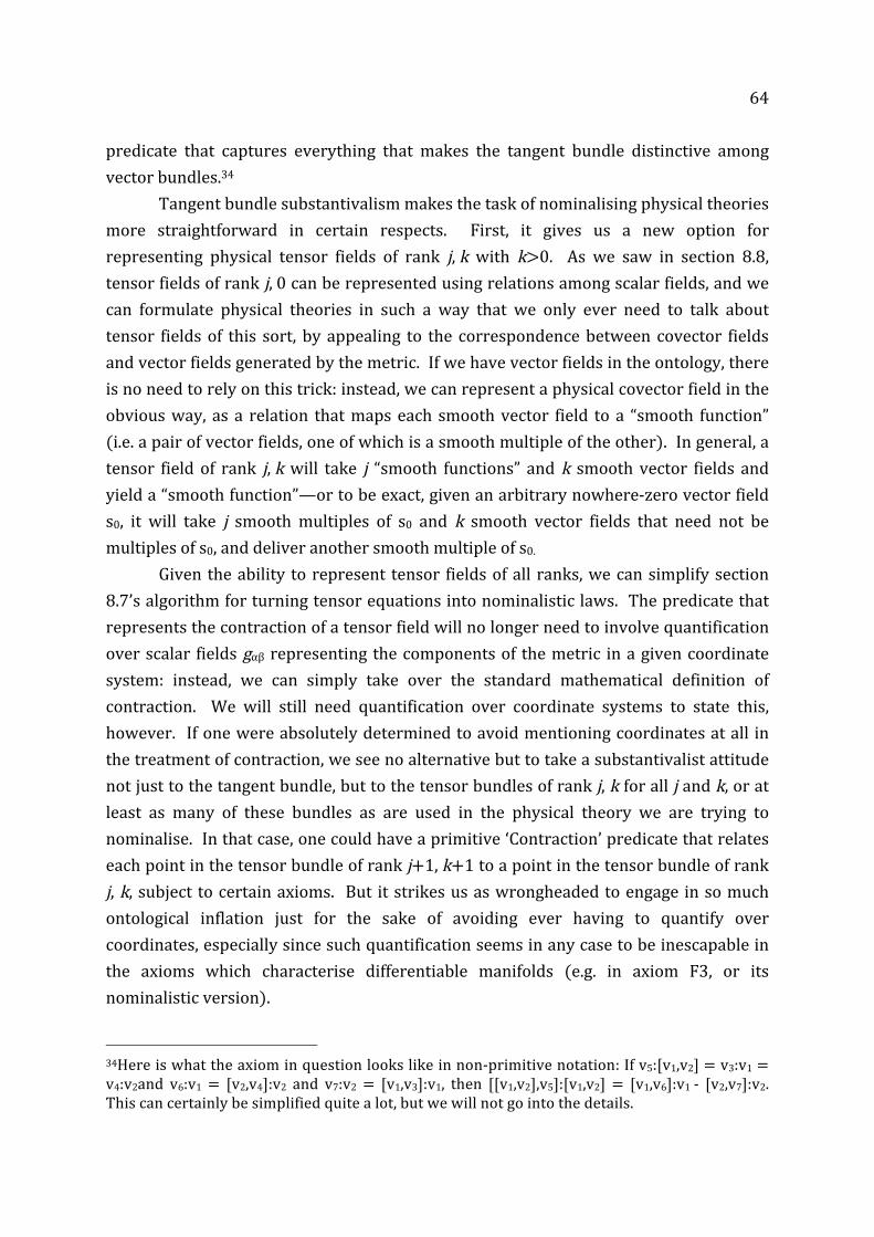
64
predicate that captures everything that makes the tangent bundle distinctive among vector bundles.34
Tangent bundle substantivalism makes the task of nominalising physical theories more straightforward in certain respects. First, it gives us a new option for representing physical tensor fields of rank j, k with k>0. As we saw in section 8.8, tensor fields of rank j, 0 can be represented using relations among scalar fields, and we can formulate physical theories in such a way that we only ever need to talk about tensor fields of this sort, by appealing to the correspondence between covector fields and vector fields generated by the metric. If we have vector fields in the ontology, there is no need to rely on this trick: instead, we can represent a physical covector field in the obvious way, as a relation that maps each smooth vector field to a “smooth function” (i.e. a pair of vector fields, one of which is a smooth multiple of the other). In general, a tensor field of rank j, k will take j “smooth functions” and k smooth vector fields and yield a “smooth function”—or to be exact, given an arbitrary nowhere-‐zero vector field s0, it will take j smooth multiples of s0 and k smooth vector fields that need not be multiples of s0, and deliver another smooth multiple of s0.
Given the ability to represent tensor fields of all ranks, we can simplify section 8.7’s algorithm for turning tensor equations into nominalistic laws. The predicate that represents the contraction of a tensor field will no longer need to involve quantification over scalar fields gαβ representing the components of the metric in a given coordinate system: instead, we can simply take over the standard mathematical definition of contraction. We will still need quantification over coordinate systems to state this, however. If one were absolutely determined to avoid mentioning coordinates at all in the treatment of contraction, we see no alternative but to take a substantivalist attitude not just to the tangent bundle, but to the tensor bundles of rank j, k for all j and k, or at least as many of these bundles as are used in the physical theory we are trying to nominalise. In that case, one could have a primitive ‘Contraction’ predicate that relates each point in the tensor bundle of rank j+1, k+1 to a point in the tensor bundle of rank j, k, subject to certain axioms. But it strikes us as wrongheaded to engage in so much ontological inflation just for the sake of avoiding ever having to quantify over coordinates, especially since such quantification seems in any case to be inescapable in the axioms which characterise differentiable manifolds (e.g. in axiom F3, or its nominalistic version).
34Here is what the axiom in question looks like in non-‐primitive notation: If v5:[v1,v2] = v3:v1 = v4:v2and v6:v1 = [v2,v4]:v2 and v7:v2 = [v1,v3]:v1, then [[v1,v2],v5]:[v1,v2] = [v1,v6]:v1 -‐ [v2,v7]:v2. This can certainly be simplified quite a lot, but we will not go into the details.

65
One other nice thing about tangent bundle substantivalism is that it gives us several natural ways of introducing a primitive predicate representing a connection on the tangent bundle—all the strategies for representing connections on general vector bundles considered in section 8.8 work just as well when the vector bundle is the tangent bundle. Since the spacetime connection is fully determined by the metric, it is not indispensable to have a primitive predicate which represents it. However, having such a predicate will probably allow for simpler formulations of the laws, and will certainly allow our nominalistic versions of the laws to follow their platonistic counterparts more closely.35
If we are not dealing with a gauge field theory, so that we don’t have any independent motivation for substantivalism about some other vector bundle, the special properties of the tangent bundle make it an especially attractive candidate to provide the vector bundle structure we need for capturing the differential structure of spacetime. Even if we are trying to nominalise a gauge field theory, so that we have an independent reason to be substantivalists about some other vector bundle, it might be worth taking a substantivalist view of the tangent bundle in addition, in view of the simplifications in the statements of physical laws which this would allow. The relative merits here depend on delicate issues about the tradeoff between simplicity in the statement of laws and ontological economy, concerning which we have no firm general views.
8.11 Further possible simplifications
As we have developed the ontology of fibre bundle substantivalism, sections are mereological fusions: the atoms of the mereology are points in fibre bundles. This is not the most ontologically economical way of proceeding. We can make the ontology smaller by throwing away the points, and instead taking the sections as the atoms of the mereology.36 The work previously done by spacetime points considered as certain fusions of fibre-‐points could be taken over by certain special sections, or fusions of sections. For example, we might identify a spacetime point with the fusion of all
35 See note 25. Even without the ontology of tangent bundle substantivalism, we might consider representing a connection using a polyadic primitive predicate of scalar fields—something like “the covariant derivative with respect to the gradient of f0 of the g1 grad f1+…+g4 grad f4 = h1 grad f1+…+h1 grad f4” (where grad f is Φg−1(df)). Or our primitive predicate could express a function from a quadruple of scalar fields (representing a coordinate system) to the components of the connection with respect to those coordinates (the Christoffel symbols). However, tangent bundle substantivalism makes it possible to use primitive predicates that are less artificial-‐looking, and have fewer argument places. 36 Dorr (2011) considers this approach in a bit more detail.

66
sections that are zero at that point. Two sections s1 and s2 “have the same value” at a spacetime point iff s1−s2 is part of that spacetime point.37 Since we have not just Smooth sections to play with, but also highly un-‐Smooth sections (e.g. sections that are zero everywhere except for one spacetime point, which can do almost all the work previously done by the points of fibre bundles), it would not be a technically difficult matter to rewrite the axioms in such a way as to work in this alternative ontological scheme. On this approach, the primitive predicates can all be taken to be predicates of mereological atoms. Because of this, a further simplification becomes available, in which we get rid of the mereological element of the theory altogether and have nothing but sections in the fundamental ontology. For this to work, we will need to be tolerant of something like plural or second order quantification: this will be needed in order to take over the crucial work that quantification over “multifields” played in the statement of axioms SN1 and SN3 (in particular, in defining what it is for one section to be a “C∞ relative to” certain other sections). If such quantification is legitimate, then quantification over mereological fusions of sections is redundant from the point of view of the project of nominalising physics. (Some think that mereological fusions “come for free”, so that there is nothing to be gained by abandoning them. We disagree.)38 Having eliminated everything except for sections (and perhaps fusions of sections) from the ontology, it is tempting to venture even further, by eliminating all the non-‐smooth sections in addition. For the special case of smooth sections in scalar value space, this kind of ontology has been considered under the name ‘Einstein Algebras’ by Robert Geroch (1972) and under the name ‘Leibniz Algebras’ by John Earman (1989, sect. 9.9). However, the challenges facing such an approach are daunting. If we cannot quantify over all sections, how can we nominalistically express the content of axiom F1, i.e. that ‘C∞ functions of smooth sections are smooth’? If we had access to all the resources of set theory, we could reconstruct such quantification using quantification
37 We can pick out the fusions that are spacetime points in this schema as the “maximal ideals”—fusions with the property that (i) whenever two sections are part of them, their sum is part of them, and (ii) whenever s1 and s2 are part of them, any other sections s3 and s4 such that s1:s2=s3:s4 are also part of them, and (iii) which are not parts of any other fusions satisfying (i) and (ii), except for the fusion of all sections. 38 By contrast, in order to replace quantification over mereological fusions of fibre-‐points with plural or second-‐order quantification, one would need to allow for primitive predicates (such as ‘Smooth’) to take plural or second-‐order arguments: we would speak of some points as “collectively” Smooth in a way that doesn’t require there to be such a thing as the “collection” of those points. The question whether primitive predicates of this sort are even intelligible raises deep foundational issues. Even if one regarded them as intelligible, one might still think that they introduced a kind of complexity which we would be better off avoiding by introducing something like mereology.

67
over ordered pairs of spacetime points and sections, where points are in turn constructed as sets of sections. And if we were completely blasé about using higher-‐order logic, we could do something similar within that framework, which might arguably be counted as nominalistic. But this would take us quite far from the kind of nominalisation project in which we have been engaged in this chapter.
8.12 Conclusions
The strategies we have presented allow for the nominalisation of a wide range of modern theories in fundamental physics. There is still work to be done, since we haven’t said anything in this chapter about the nominalisation of quantum theories. However, it seems to us that the main problem here is simply the one that was discussed in Chapter 3 of this book: that of finding a satisfactory account of what quantum theories are telling us about the fundamental structure of the world. We want to be able to understand these theories not just as pragmatic devices for predicting the outcomes of experiments, but as accounts of what there is, fundamentally speaking, and of the pattern of fundamental properties and relations. Once one has given a clear and satisfactory account of the fundamental structure of the world according to quantum theory, we foresee no distinctively new obstacles to the project of nominalising such an account. For example, one view takes the wavefunction over configuration space as a straightforward representation of the fundamental structure of the world. On this view, the fundamental ontology includes entities standing in some geometric relations that make it natural to think of them as “points of configuration space”, and standing in some other relations that pick out a function from them to the complex numbers as “the wavefunction” (or to be more precise, that pick out a certain small equivalence class of functions from them to the complex numbers as “legitimate choices of wavefunction”). The techniques required for nominalising classical field theories should extend quite easily to theories of this sort. Other accounts of the fundamental ontology of quantum theories will involve a similarly “substantivalist” attitude towards other high-‐dimensional spaces: the Hilbert space, the space of operators, or some interesting subspaces of the space of operators such as the space of field-‐configuration operators. Again, with such a richly structured domain of concrete entities to work with, nominalisation seems unlikely to be very difficult. The dialectical situation seems quite similar to the case of classical gauge field theories: the richly structured ontology of concrete objects which makes nominalisation feasible can be motivated quite independently of any commitment to nominalism, simply by the demand for a satisfactory account of the concrete facts upon which the phenomena supervene.

68
One might think that, e.g., a Hilbert space is a paradigm mathematical object, so that no theory positing such a thing could count as genuinely “nominalistic”. But as we have already said, we don’t want to quibble about the label. We are simply interested in the question which entities exist, and how they are structured. We take it that our best theories of the phenomena are our best guide to answering this question, and that a parsimonious, simple theory is more likely to be true than a complex, rich theory. Since the mathematical realm, as conceived by those who believe in it, contains instantiations of more or less every possible structure, any answer we might come up with will have the feature that according to it, the structure of the concrete world is isomorphic to that of some (putative) mathematical entity. It may strike some readers that the theories we have been developing are much more complex than familiar platonistic ones, so that even by our own standards, we should be willing, for the sake of having simple laws, to embrace the mathematical ontology those theories require. We disagree: much of the complexity of platonistic theories is hidden behind a hierarchy of definitions, which practitioners rarely have any need to consult.
But even if it is true that there are some additions to the ontology we have been advocating that can be justified by gains in simplicity, we think it is a mistake to think of mathematical ontology as an all-‐or-‐nothing deal. Otherwise we might as well have thrown in the towel at the point when Sumerians first discovered how to use abacuses to keep track of the size of their herds! Mathematics is a stupendously useful tool. It describes and systematises a vast array of possible structures, any one of which we might find ourselves having reason to ascribe to part of the real world. We should feel free to avail ourselves of these options, without fearing that once we start doing so, we will somehow end up having to believe that every one of those structures is instantiated somewhere in reality.

69
APPENDICES
Appendix A: Different differential structures that generate the same embedded subregions
Let D be the standard differential structure on ℝ2. Let D′ be the non-‐standard structure such that a function f is smooth according to D′ iff f∘Φ is smooth according to D. We will show that for any set S, S is the image of a smooth embedding of a one-‐dimensional manifold into D iff S is the image of a smooth embedding of a one-‐dimensional manifold into D′. Since D and D′ disagree only at <0,0>, it suffices to consider curves γ: (−1,1)→ℝ2 with γ(0)=<0,0> and γ′(0) nonzero (as required for γ to be an embedding).39 Lemma 1: A curve γ (function from ℝto ℝ2) is smooth according to D′ iff Φ-‐1∘γ is smooth according to D. Proof: A curve is smooth iff its composition with any smooth function is smooth. But if f is smooth according to D′, it is of the form g∘Φ−1 with g smooth according to D. So γ is smooth according to D′ iff f∘Φ−1∘γ is smooth according to D for every smooth f. This entails that Φ−1∘γ is smooth (taking f to be the identity function), and since composition of smooth functions preserves smoothness, it is also entailed by Φ−1∘γ being smooth. Corollary: If γ is smooth according to D′, it is smooth according to D. Lemma 2: Suppose γ(t) is a function from [−1,1] to ℝ2 such that γ(0)=<0,0> and γ′(0) is nonzero. Then if γ is smooth according to D, γ(t3) is smooth according to D′. Proof: We will show that Φ-‐1(γ(t3)) is smooth according to D; this is sufficient for γ(t3) to be smooth according to D′ by Lemma 1.
Let γ(t) = <f(t),g(t)>. Since γ′(0) is nonzero, we know that either f′(0) or g′(0) is nonzero; without loss of generality, let us suppose f′(0) is nonzero. Then when t≠0,
Φ-‐1(f(t3)) = <f(t3)/((f(t3))2+(g(t3))2)1/3, g(t3)/((f(t3))2+(g(t3))2)1/3>
Define f*(t)=f(t3)/t3 when t≠0, f*(0) = 6f′(0); g*(t)=g(t3)/t3 when t≠0, g*(0)=6g′(0). Then when t≠0,
Φ-‐1(f(t3)) = <t∙f*(t)/((f*(t))2+(g*(t))2)1/3, t∙g*(t)/((f*(t))2+(g*(t))2))1/3>
39 This proof is essentially due to Teru Thomas.

70
To show that this is smooth at 0, it is sufficient—since the product of two smooth functions is smooth, and the quotient of two smooth functions is smooth wherever the denominator is nonzero, and any power of a smooth function is smooth wherever that function is nonzero—to show that f* and g* are smooth at 0, and that f* is nonzero at 0 (since in that case (f*(t))2 must be positive at 0, and hence so must (f*(t))2+(g*(t))2) and ((f*(t))2+(g*(t))2))1/3).
To show that f* and g* are smooth at 0, we use the fact—which can be verified by manipulating the epsilon-‐delta definition of differentiation—that if the first two derivatives of a smooth function h(t) vanish at 0, then the function j defined by j(t)=h(t)/t3, j(0)=h′(0) is also smooth at 0. The first two derivatives of f(t3) and g(t3) do vanish at 0, since
d/dt f(t3)|0 = 3f′(t3)t2 |0 = 0
d2/dt2 f(t3)|0 = 9f′′(t3)t4+6f′(t3)t|0 = 0 and similarly for g. And the third derivative of f(t3) and g(t3) are respectively equal to 6f′(0) and 6g′(0), since
d3/dt3 f(t3)|0 = 27f′′′(t3)t6+36f′′(t3)t3+18f′′(t3)t+6f′(t3)|0 = 6f′(0) and similarly for g. This tells us that f* and g* are smooth at 0; also, since f′(0)≠0, we have that f*(0) is nonzero, as required. Corollary: for any set S, if according to D, S is the image of a function γ:[−1,1]→ℝ2 with γ(0)=<0,0> and γ′(0) nonzero, then this is also the case according to D′, and conversely.
Appendix B: ‘Diag’ determines differential structure
In this appendix we will show that if we have differential structures D and D′ on a topological manifold of dimension at least two, and they agree on the extension of the predicate Diag(R1,R2,R3) defined as follows:
For some smooth functions x and y and open region O such that x and y form part of an admissible coordinate system mapping O onto a convex open subset of ℝn:

71
R1 comprises exactly the points where x is rational, and R2 comprises exactly the points where y is rational, and R3 comprises exactly the points where x=y.
then D=D′. Lemma 3: If f and g are continuous functions on an open region O, and for every x, the subregions f=x and g=x of O are connected, and the points in O where the value of f is rational are exactly those where the value of g is rational, then there is a continuous function h: ℝ→ℝ such that f =h(g). Proof. Suppose we had two points a and b in O such that g(a)=g(b) but f(a)≠f(b). Let r be a rational number between f(a) and f(b). Since f is continuous, every path from a to b must pass through a point where f=r. Since the region where g=g(a) is connected, no path from a to b has to pass through a point where the value of g is anything other than g(a). But g is rational whenever f=r. So g(a) must be rational. So f(a) and f(b) must be rational. But then there is some irrational number x between f(a) and f(b). Since f is continuous, every path from a to b has to pass through a point where f=x. But g is irrational whenever f=x. So every path from a to b has to pass through a point where g is irrational. This cannot be the case, since g(a)=g(b) is rational the set of points where g=g(a) is connected. Lemma 4: Suppose D is a differentiable structure, and x and y form part of a convex coordinate system on an open region O that is admissible according to D. Let R1 comprise the points where x is rational and R2, the points where y is rational. Then for any region R3, Diag(R1,R2,R3) iff for some diffeomorphism f on the real line, R3 comprises the points where y=f(x). Proof. Left-‐to-‐right: if Diag(R1,R2,R3), there is a D-‐admissible convex coordinate system x′,y′ such that x′ is rational exactly in R1, y′ is rational exactly in R2, and x′=y′ exactly in R3. Since x and x′ both form parts of convex coordinate systems on O, both are continuous, and their level sets within O must all be connected. So by Lemma 3, x′ must equal g(x) for some g: ℝ→ℝ. Similarly, y′ must equal h(y) for some h: ℝ→ℝ. Since x′ and y′ are part of an admissible coordinate system, g and h must be diffeomorphisms. Since R3 comprises the points where y′=x′, it comprises the points where y=h-‐1(g(x)); so h-‐1∘g is a diffeomorphism f as required.
Right-‐to-‐left: suppose f is a diffeomorphism on the real line, and R3 comprises the points where y=f(x). If x and y form part of a convex coordinate system on O that is admissible according to D, so do x′=f(x) and y. (Applying f to one coordinate while
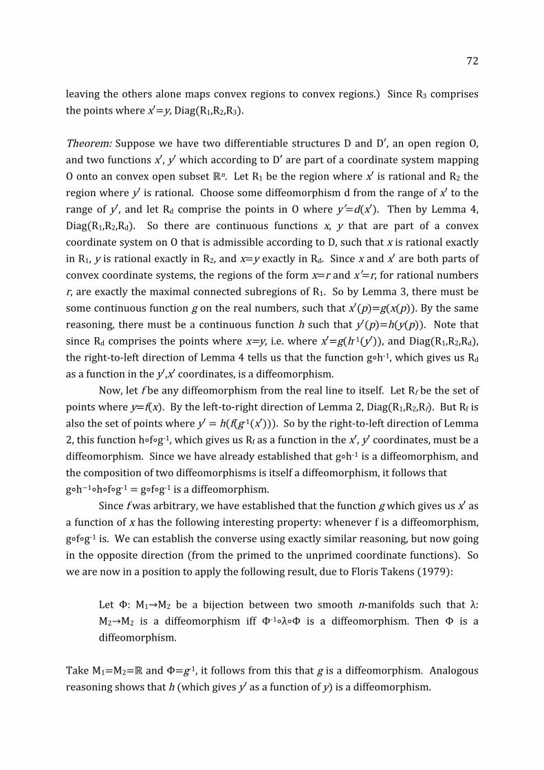
72
leaving the others alone maps convex regions to convex regions.) Since R3 comprises the points where x′=y, Diag(R1,R2,R3). Theorem: Suppose we have two differentiable structures D and D′, an open region O, and two functions x′, y′ which according to D′ are part of a coordinate system mapping O onto an convex open subset ℝn. Let R1 be the region where x′ is rational and R2 the region where y′ is rational. Choose some diffeomorphism d from the range of x′ to the range of y′, and let Rd comprise the points in O where y′=d(x′). Then by Lemma 4, Diag(R1,R2,Rd). So there are continuous functions x, y that are part of a convex coordinate system on O that is admissible according to D, such that x is rational exactly in R1, y is rational exactly in R2, and x=y exactly in Rd. Since x and x′ are both parts of convex coordinate systems, the regions of the form x=r and x′=r, for rational numbers r, are exactly the maximal connected subregions of R1. So by Lemma 3, there must be some continuous function g on the real numbers, such that x′(p)=g(x(p)). By the same reasoning, there must be a continuous function h such that y′(p)=h(y(p)). Note that since Rd comprises the points where x=y, i.e. where x′=g(h-‐1(y′)), and Diag(R1,R2,Rd), the right-‐to-‐left direction of Lemma 4 tells us that the function g∘h-‐1, which gives us Rd as a function in the y′,x′ coordinates, is a diffeomorphism.
Now, let f be any diffeomorphism from the real line to itself. Let Rf be the set of points where y=f(x). By the left-‐to-‐right direction of Lemma 2, Diag(R1,R2,Rf). But Rf is also the set of points where y′ = h(f(g-‐1(x′))). So by the right-‐to-‐left direction of Lemma 2, this function h∘f∘g-‐1, which gives us Rf as a function in the x′, y′ coordinates, must be a diffeomorphism. Since we have already established that g∘h-‐1 is a diffeomorphism, and the composition of two diffeomorphisms is itself a diffeomorphism, it follows that g∘h−1∘h∘f∘g-‐1 = g∘f∘g-‐1 is a diffeomorphism.
Since f was arbitrary, we have established that the function g which gives us x′ as a function of x has the following interesting property: whenever f is a diffeomorphism, g∘f∘g-‐1 is. We can establish the converse using exactly similar reasoning, but now going in the opposite direction (from the primed to the unprimed coordinate functions). So we are now in a position to apply the following result, due to Floris Takens (1979):
Let Φ: M1→M2 be a bijection between two smooth n-‐manifolds such that λ: M2→M2 is a diffeomorphism iff Φ-‐1∘λ∘Φ is a diffeomorphism. Then Φ is a diffeomorphism.
Take M1=M2=ℝ and Φ=g-‐1, it follows from this that g is a diffeomorphism. Analogous reasoning shows that h (which gives y′ as a function of y) is a diffeomorphism.

73
So we have established that the coordinates x′, y′, which are admissible according to differential structure D′, are also admissible according to differential structure D. This means that in general, any convex coordinatisation of an open neighbourhood that is admissible according to D′ is admissible according to D. And the reverse is true too (by isomorphic reasoning). But if so, D and D′ must be the same differential structure: for if any coordinate system were admissible according to one but not the other, some of its restrictions to convex regions of ℝn would have to be admissible according to the one but no the other, admissibility being a local matter. So from the assumption that D and D′ agree about the extension of Diag, we have deduced that they are the same differential structure.40
Appendix C: Adequacy of our axioms for scalar value lines
In this appendix we will sketchily prove the following representation theorem: in any model of M1−M5 (second-‐order classical mereology+atomicity), A1−A6 (‘addition is an abelian group on each scalar value line’) and P1−P6 (repeated below), and every scalar value line l in that model, there is a unique function πl from the real numbers to points in u’s scalar value line such that πl(α+β)=πl(α)+πl(β), πl(α) is Positive iff α>0, and πl(α) is a Unit iff α=1. And this πl is one-‐to-‐one. P1 Everything Positive lacks proper parts P2 If x and y are Positive, x+y is Positive (i.e. ‘< is transitive’, where ‘x<y’ means
‘x−y is Positive’.) P3 Whenever x is Positive, −x is not Positive. (‘≤ is antisymmetric’) P4 Whenever x is atomic and not zero, either x or −x is Positive. (‘≤ is total’) P5 If x is Positive, there exist Positive y and z such that Sum(y,z,x). (‘≤ is dense’) P6 If X<Y, then there is a z such that X≤z and z≤Y. (‘≤ is Dedekind complete’:
X<Y means ‘whenever x is an atomic part of X and y is an atomic part of Y, x<y’.)
We will need a lemma: Lemma 5: For every x, there is exactly one y such that y+…+y [m terms]=x. Proof. Let S be the fusion of points s such that s+…+s≤x, and B the fusion of b such that b+…+b>x. S<B, since if x>y, x+…_+x>y+…+y by P2. So by P6 there is a z such that
40 Thanks to Andrew Stacey for pointing us to the Takens result and explaining its relevance to our question.

74
S≤z and z≤B. Now, suppose that z+…_+z>y. Then by P5, there is a w such that 0<w<z+…+z−y. By repeated applications of P5, w=w1+…+wm for some Positive w1,…,wm. Let wi be the smallest of w1,…,wm; then wi+…+wi≤w. So (z+…+z)−(wi+…+wi)≥(z+…+z)−w>y. Hence z-‐wi belongs to B, contradicting our assumption. The possibility that z+…+z<y can be ruled out by similar reasoning, leaving z+…+z=y the only possibility by P4. Could there be some other z’ such that z′+…+z′=y? No: if z+…+z=z′+…+z′, then (z−z′)+…+(z−z′) is zero, which by P2 could not happen if z−z′ or z′−z were Positive. We are now in a position to prove our representation theorem.
(i) Existence. We start by defining πinductively for integers, by requiring that πl(1) be the unique Unit of l, and that πl(n+m)=πl(n)+πl(m) and πl(n−m)=πl(n)−πl(m). When α is a rational number of the form n/m (where m is positive), we let πl(α) be the point z such that z+…+z [m terms]=πl(n), which exists by Lemma 5. This extension of π will obviously still respect the addition facts. Finally, when α is irrational, we let πl(α) be the point z such that X≤z and z≤Y, where X is the fusion of points πl(n/m) where n/m< α, and Y is the fusion of points πl(n/m) where n/m>α. By P6, there is such a z. Showing thaton this definition πl(α)+πl(β)=πl(α+β) comes down to showing that whenever x<y, x<πl(n/m)<y for some n and m. For this, we use P6 to show that every Positive z is greater than some point of the form πl(1/m), and then argue inductively that if so, some point of the form πl(n/m) must occur between any two points whose difference is at least z.
(ii) Uniqueness. Suppose πl and ρl both meet the specified conditions. By induction, πl(n)=ρl(n) for each integer n. If α is a rational number n/m (m positive), we have that πl(α)+…+πl(α) [m terms]=πl(n)=ρl(n)=ρl(α)+…+ρl(α); but if πl(α)<ρl(α), P2 tells us that πl(α)+…+πl(α)<ρl(α)+…+ρl(α) and hence πl(α)+…+πl(α)≠ρl(α)+…+ρl(α) (by P3). And since πl and ρl both respect the ordering facts, they must also agree on the points they assign to irrational numbers, again using the fact that any two points are separated by some point of the form πl(n/m).
(iii) One-‐to-‐oneness: First, since πl(α)+πl(β)=πl(α+β), πl(0)+πl(0)=πl(0), so πl(0) is zero. We first show that πl(α) is not zero for any other α. First, πl(α)+πl(−α) is zero for every α, so πl(−α)=−πl(α), so it suffices to show that πl(α) is not zero for any Positive α. Suppose otherwise. Then for some m, mα≥1; so, arguing inductively, and appealing to the fact that πl respects ordering facts, πl(α)+…+πl(α) [m terms]≥πl(1). But πl(1) is the Unit of l, which is Positive by U2; so by P2 πl(α)+…+πl(α) is Positive. This cannot happen if πl(α) is zero, by P3.

75
Suppose then that πl(α) = πl(β). Then πl(α)−πl(β) is zero, so πl(α)+πl(−β) is zero, so πl(α−β) is zero, so α−β is zero by the result we just proved. So α=β, proving that πl is one-‐to-‐one.
Appendix D: Nominalistic treatment of vector spaces
In this appendix we prove a representation theorem: in any model of axioms M1−M5 (classical mereology), A1−A6 (‘addition is an abelian group on each fibre’) and SD1−SD9 (given in section 8.9, and repeated here for convenience), there is a unique way of assigning each fibre the structure of a vector space over the real numbers, in such a way that SameDirection(x,y) iff x=αy for some positive real number α. SD1 If SameDirection(v, x), then v and x lack proper parts SD2 If SameDirection(v, x) and SameDirection(v, y), SameDirection(v, x+y) SD3 If v is nonzero and SameDirection(v, x), then not SameDirection(v, −x) SD4 Whenever x is a nonzero multiple of v, either SameDirection(v, x) or
SameDirection(v, −x) SD5 For any v, there exist x and y such that x+y=v and SameDirection(v, x) and
SameDirection(v, y) SD6 If X and Y are fusions of multiples of v and X<vY, then there is a multiple z of v
such that X≤vz and z≤vY. SD7 SameDirection is symmetric, transitive, and reflexive on nonzero vectors SD8 SameDirection(−v1, −v2) whenever SameDirection(v1,v2) SD9 If SameDirection(v+w,x), then for some y and z such that y+z=x,
SameDirection(v,y) and SameDirection(w,z). Here ‘x is a multiple of y’ means ‘for some z1 and z2 SameDirection(y,z1) and SameDirection(y,z2) and x=z1+z2’. Lemma 6: x+…+x = y+…+y only whenx=y. Proof. Suppose x+…+x = y+…+y. If x is zero, then x+…+x = y+…+y is zero. But then y must be zero, since otherwise we would have SameDirection(y,y) by SD7, and hence SameDirection(y,y+…+y) by SD2, and hence SameDirection(y+…+y,y) by SD7, and SameDirection(y+…+y,y+…+y) by SD2 again, contradicting SD3. Similarly, if y is zero, x must be. So we can assume that neither x nor y is zero. Then SameDirection(x,x) and SameDirection(y,y) by SD7. So by SD2, SameDirection(x,x+…+x) and SameDirection(y,y+…+y). So by transitivity (SD7), SameDirection(x,y). Then since x−y is a multiple of x, SD4 tells us that either SameDirection(x,x−y) or
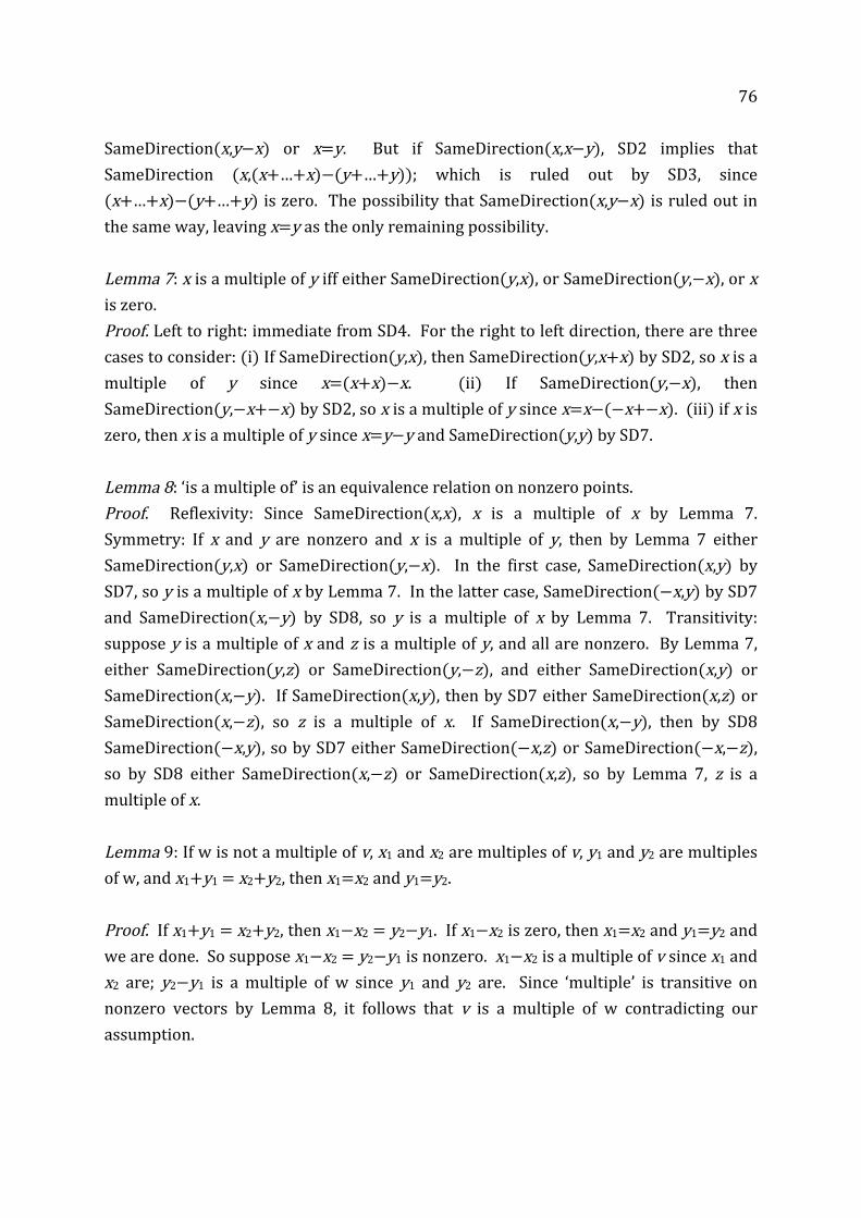
76
SameDirection(x,y−x) or x=y. But if SameDirection(x,x−y), SD2 implies that SameDirection (x,(x+…+x)−(y+…+y)); which is ruled out by SD3, since (x+…+x)−(y+…+y) is zero. The possibility that SameDirection(x,y−x) is ruled out in the same way, leaving x=y as the only remaining possibility. Lemma 7: x is a multiple of y iff either SameDirection(y,x), or SameDirection(y,−x), or x is zero. Proof. Left to right: immediate from SD4. For the right to left direction, there are three cases to consider: (i) If SameDirection(y,x), then SameDirection(y,x+x) by SD2, so x is a multiple of y since x=(x+x)−x. (ii) If SameDirection(y,−x), then SameDirection(y,−x+−x) by SD2, so x is a multiple of y since x=x−(−x+−x). (iii) if x is zero, then x is a multiple of y since x=y−y and SameDirection(y,y) by SD7. Lemma 8: ‘is a multiple of’ is an equivalence relation on nonzero points. Proof. Reflexivity: Since SameDirection(x,x), x is a multiple of x by Lemma 7. Symmetry: If x and y are nonzero and x is a multiple of y, then by Lemma 7 either SameDirection(y,x) or SameDirection(y,−x). In the first case, SameDirection(x,y) by SD7, so y is a multiple of x by Lemma 7. In the latter case, SameDirection(−x,y) by SD7 and SameDirection(x,−y) by SD8, so y is a multiple of x by Lemma 7. Transitivity: suppose y is a multiple of x and z is a multiple of y, and all are nonzero. By Lemma 7, either SameDirection(y,z) or SameDirection(y,−z), and either SameDirection(x,y) or SameDirection(x,−y). If SameDirection(x,y), then by SD7 either SameDirection(x,z) or SameDirection(x,−z), so z is a multiple of x. If SameDirection(x,−y), then by SD8 SameDirection(−x,y), so by SD7 either SameDirection(−x,z) or SameDirection(−x,−z), so by SD8 either SameDirection(x,−z) or SameDirection(x,z), so by Lemma 7, z is a multiple of x. Lemma 9: If w is not a multiple of v, x1 and x2 are multiples of v, y1 and y2 are multiples of w, and x1+y1 = x2+y2, then x1=x2 and y1=y2. Proof. If x1+y1 = x2+y2, then x1−x2 = y2−y1. If x1−x2 is zero, then x1=x2 and y1=y2 and we are done. So suppose x1−x2 = y2−y1 is nonzero. x1−x2 is a multiple of v since x1 and x2 are; y2−y1 is a multiple of w since y1 and y2 are. Since ‘multiple’ is transitive on nonzero vectors by Lemma 8, it follows that v is a multiple of w contradicting our assumption.

77
Theorem: In any model of the axioms, whenever v is nonzero, there is a unique function πv from real numbers to vectors with the properties that (a) πv(1)=v, (b) πv(α+β)=πv(α)+πv(β), and (c) SameDirection(v,πv(α)) iff α>0. And this function is one-‐to-‐one. Proof. From the theorem of Appendix C, noting that P1−P6 and U1−U2 are true when we restrict all quantifiers to multiples of v, interpret ‘Positive(x)’ as ‘SameDirection(v,x)’ and ‘Unit(x)’ as ‘x=v’. Theorem: The operation ‘x = αv’ defined by ‘eitherv is nonzero andπv(α) = x, or vis zero and x=v’ satisfies the axioms for scalar multiplication in a vector space, i.e.: (i) 1v = v (ii) (α+β)v = αv+βv (iii) α(βv) = (αβ)v (iv) α(v+w) = αv+αw
Proof. (i) and (ii) are immediate from the properties (a) and (b) of πv. For (iii), there are four cases to consider. Case 1: v is zero; then both sides are zero. Case 2: v is nonzero and β=0. Then v=(1+β)v=v+βv, so βv is zero, so α(βv) is zero.
And (αβ)v = 0v = (1−1)v=v−v, which is also zero. Case 3: v is nonzero and β>0. Then SameDirection(v,βv) by (c). By SD7, for any x,
SameDirection(v,x) iff SameDirection(βv,x). So 0<πv(x) iff 0<πβv(x). And more generally, πv(x)≤πv(y) iff πβv(x)≤πβv(y). Also, by Lemma 8, the multiples of v are exactly the multiples of βv. We know that πβv is the one and only additive function from the multiples of βv to the reals such that π(βv)=1 and πβv(x)≤πβv(y) whenever x≤βvy. But we have just seen that the function f(x):= πv(x)/β has exactly these properties. So in general, πβv(x) = πv(x)/β. In other words, x=α(βv) iff x = (αβ)v.
Case 4: v is nonzero and β<0. Then SameDirection(v,−βv). By SD7 and SD8, for any x, SameDirection(v,x) iff SameDirection(βv,−x). So 0<πv(x) iff 0<πβv(−x) which is true iff πβv(x)<0. More generally, πv(x)≤πv(y) iff πβv(y)≤πβv(x). Also, by Lemma 8, the multiples of v are exactly the multiples of βv. Thus as in Case 3, the function f(x):=πv(x)/β has exactly the properties that we know are unique to πβv.
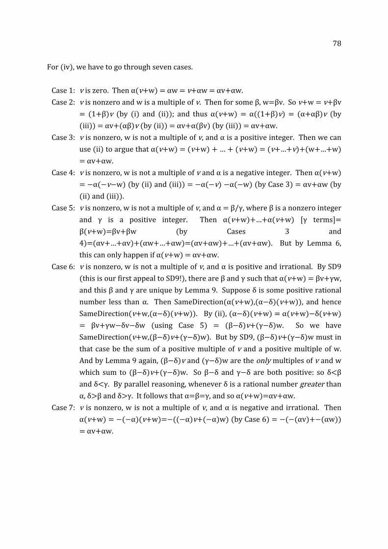
78
For (iv), we have to go through seven cases. Case 1: v is zero. Then α(v+w) = αw = v+αw = αv+αw. Case 2: v is nonzero and w is a multiple of v. Then for some β, w=βv. So v+w = v+βv
= (1+β)v (by (i) and (ii)); and thus α(v+w) = α((1+β)v) = (α+αβ)v (by (iii)) = αv+(αβ)v (by (ii)) = αv+α(βv) (by (iii)) = αv+αw.
Case 3: v is nonzero, w is not a multiple of v, and α is a positive integer. Then we can use (ii) to argue that α(v+w) = (v+w) + … + (v+w) = (v+…+v)+(w+…+w) = αv+αw.
Case 4: v is nonzero, w is not a multiple of v and α is a negative integer. Then α(v+w) = −α(−v−w) (by (ii) and (iii)) = −α(−v) −α(−w) (by Case 3) = αv+αw (by (ii) and (iii)).
Case 5: v is nonzero, w is not a multiple of v, and α = β/γ, where β is a nonzero integer and γ is a positive integer. Then α(v+w)+…+α(v+w) [γ terms]= β(v+w)=βv+βw (by Cases 3 and 4)=(αv+…+αv)+(αw+…+αw)=(αv+αw)+…+(αv+αw). But by Lemma 6, this can only happen if α(v+w) = αv+αw.
Case 6: v is nonzero, w is not a multiple of v, and α is positive and irrational. By SD9 (this is our first appeal to SD9!), there are β and γ such that α(v+w) = βv+γw, and this β and γ are unique by Lemma 9. Suppose δ is some positive rational number less than α. Then SameDirection(α(v+w),(α−δ)(v+w)), and hence SameDirection(v+w,(α−δ)(v+w)). By (ii), (α−δ)(v+w) = α(v+w)−δ(v+w) = βv+γw−δv−δw (using Case 5) = (β−δ)v+(γ−δ)w. So we have SameDirection(v+w,(β−δ)v+(γ−δ)w). But by SD9, (β−δ)v+(γ−δ)w must in that case be the sum of a positive multiple of v and a positive multiple of w. And by Lemma 9 again, (β−δ)v and (γ−δ)w are the only multiples of v and w which sum to (β−δ)v+(γ−δ)w. So β−δ and γ−δ are both positive: so δ<β and δ<γ. By parallel reasoning, whenever δ is a rational number greater than α, δ>β and δ>γ. It follows that α=β=γ, and so α(v+w)=αv+αw.
Case 7: v is nonzero, w is not a multiple of v, and α is negative and irrational. Then α(v+w) = −(−α)(v+w)=−((−α)v+(−α)w) (by Case 6) = −(−(αv)+−(αw)) = αv+αw.

79
REFERENCES
Burgess, J. and Rosen, G. (1997): A Subject with No Object. Oxford: Clarendon Press. Chevalley, C. (1946): Theory of Lie Groups. Princeton: Princeton University Press. Dorr, C. (2007): “There Are No Abstract Objects”, in T. Sider, J. Hawthorne and D.
Zimmerman (eds.): Contemporary Debates in Metaphysics: 32-‐64. Malden, Mass: Wiley-‐Blackwell.
— (2010): “Of Numbers and Electrons”. Proceedings of the Aristotelian Society 110: 133-‐181.
— (2011): “Physical Geometry and Fundamental Metaphysics”, Proceedings of the Aristotelian Society 111. Earman, J. (1989): World Enough and Space-‐time. Cambridge, Mass.: MIT Press. Field, H. (1980): Science Without Numbers. Oxford: Blackwell. — (1985b): “On Conservativeness and Incompleteness”, Journal of Philosophy 82: 239-‐
260. Galilei, G. (1623): Il Saggiatore, in Opere Vol 6. Geroch, R. (1972): “Einstein Algebras”, Communications in Mathematical Physics 26:
271-‐275. Mach, E. (1893): The Science of Mechanics. La Salle, Illinois: Open Court. Mundy, B. (1992): “Space-‐Time and Isomorphism”, Proceedings of the 1992 Biennial
Meeting of the Philosophy of Science Association, Vol. 1, pp 515-‐527. East Lansing, Michigan: Philosophy of Science Association.
Mundy, B. (1994): “Quantity, Representation and Geometry”, in P. Humphreys (ed., 1994): Patrick Suppes: Scientific Philosopher, Vol 2: 59-‐102. Berlin: Springer Verlag.
Newton, I. (1674-‐1689): The Mathematical Papers of Isaac Newton, volume 4, ed. D. T. Whiteside. New York: Johnson Reprint Corporation, 1964.
Nomizu, K. (1956): Lie Groups and Differential Geometry. Mathematical Society of Japan.
Pemberton, H. (1728): A View of Sir Isaac Newton’s Philosophy. London: S. Palmer. Penrose, R. & Rindler, W. (1984): Spinors and Space-‐Time, Volume 1. Cambridge:
Cambridge University Press. Putnam, H. (1971): Philosophy of Logic. New York: Harper and Row. Reprinted in
Mathematics, Matter and Method: Philosophical Papers, vol. 1: 323-‐-‐357. Cambridge: Cambridge University Press.
Sikorski, R. (1972): Introduction to Differential Geometry. Warszawa: Polish Scientific Publishers. (In Polish)

80
Takens, F. (1979): “Characterization of a Differentiable Structure by Its Group of Diffeomorphisms”, Bol. Soc. Bras. Mat. 10: 17-‐26.


![dl.abcbourse.irFrank_Wood]_Business... · Business Accounting Basics Frank Wood David Horner Frank Wood’s Business Accounting Basics Frank Wood David Horner Frank Wood’s Front](https://img.pdfslide.net/doc/110x75/5f5382125c13e2675439dc65/dl-frankwoodbusiness-business-accounting-basics-frank-wood-david-horner.jpg)


![[Book] Frank Zappa - Frank Zappa Songbook Vol 1](https://img.pdfslide.net/doc/110x75/568c4a5b1a28ab491697cd91/book-frank-zappa-frank-zappa-songbook-vol-1.jpg)


![[123doc.vn] ebook nhat ky anne frank anne frank](https://img.pdfslide.net/doc/110x75/5587b548d8b42a9d688b46ab/123docvn-ebook-nhat-ky-anne-frank-anne-frank.jpg)

![«The Fabulous Frank Gigliotti» [Il Favoloso Frank Gigliotti]](https://img.pdfslide.net/doc/110x75/579077f91a28ab6874c04501/the-fabulous-frank-gigliotti-il-favoloso-frank-gigliotti.jpg)