Embed Size (px)
Citation preview
Calculus I Lecture Notes
David M. McClendon
Department of MathematicsFerris State University
Spring 2017 edition
1
Contents
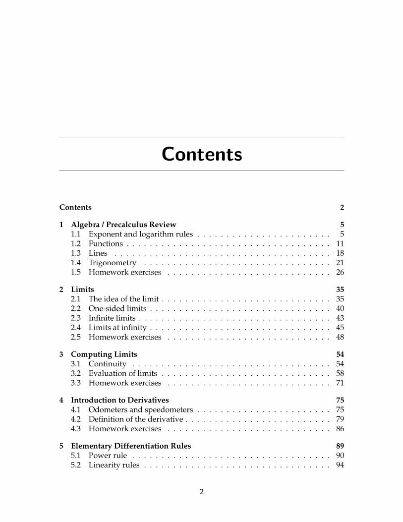
Contents 2
1 Algebra / Precalculus Review 51.1 Exponent and logarithm rules . . . . . . . . . . . . . . . . . . . . . . . 51.2 Functions . . . . . . . . . . . . . . . . . . . . . . . . . . . . . . . . . . . 111.3 Lines . . . . . . . . . . . . . . . . . . . . . . . . . . . . . . . . . . . . . 181.4 Trigonometry . . . . . . . . . . . . . . . . . . . . . . . . . . . . . . . . 211.5 Homework exercises . . . . . . . . . . . . . . . . . . . . . . . . . . . . 26
2 Limits 352.1 The idea of the limit . . . . . . . . . . . . . . . . . . . . . . . . . . . . . 352.2 One-sided limits . . . . . . . . . . . . . . . . . . . . . . . . . . . . . . . 402.3 Infinite limits . . . . . . . . . . . . . . . . . . . . . . . . . . . . . . . . . 432.4 Limits at infinity . . . . . . . . . . . . . . . . . . . . . . . . . . . . . . . 452.5 Homework exercises . . . . . . . . . . . . . . . . . . . . . . . . . . . . 48
3 Computing Limits 543.1 Continuity . . . . . . . . . . . . . . . . . . . . . . . . . . . . . . . . . . 543.2 Evaluation of limits . . . . . . . . . . . . . . . . . . . . . . . . . . . . . 583.3 Homework exercises . . . . . . . . . . . . . . . . . . . . . . . . . . . . 71
4 Introduction to Derivatives 754.1 Odometers and speedometers . . . . . . . . . . . . . . . . . . . . . . . 754.2 Definition of the derivative . . . . . . . . . . . . . . . . . . . . . . . . . 794.3 Homework exercises . . . . . . . . . . . . . . . . . . . . . . . . . . . . 86
5 Elementary Differentiation Rules 895.1 Power rule . . . . . . . . . . . . . . . . . . . . . . . . . . . . . . . . . . 905.2 Linearity rules . . . . . . . . . . . . . . . . . . . . . . . . . . . . . . . . 94
2
Contents
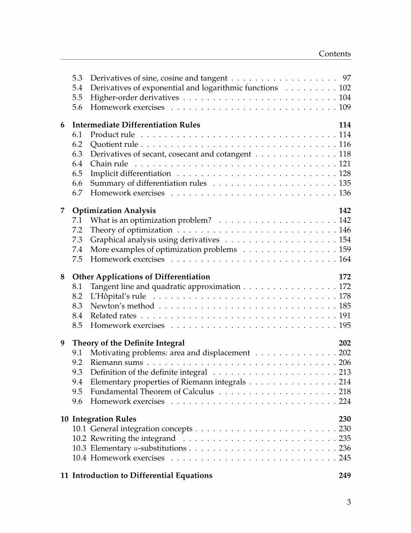
5.3 Derivatives of sine, cosine and tangent . . . . . . . . . . . . . . . . . . 975.4 Derivatives of exponential and logarithmic functions . . . . . . . . . 1025.5 Higher-order derivatives . . . . . . . . . . . . . . . . . . . . . . . . . . 1045.6 Homework exercises . . . . . . . . . . . . . . . . . . . . . . . . . . . . 109
6 Intermediate Differentiation Rules 1146.1 Product rule . . . . . . . . . . . . . . . . . . . . . . . . . . . . . . . . . 1146.2 Quotient rule . . . . . . . . . . . . . . . . . . . . . . . . . . . . . . . . . 1166.3 Derivatives of secant, cosecant and cotangent . . . . . . . . . . . . . . 1186.4 Chain rule . . . . . . . . . . . . . . . . . . . . . . . . . . . . . . . . . . 1216.5 Implicit differentiation . . . . . . . . . . . . . . . . . . . . . . . . . . . 1286.6 Summary of differentiation rules . . . . . . . . . . . . . . . . . . . . . 1356.7 Homework exercises . . . . . . . . . . . . . . . . . . . . . . . . . . . . 136
7 Optimization Analysis 1427.1 What is an optimization problem? . . . . . . . . . . . . . . . . . . . . 1427.2 Theory of optimization . . . . . . . . . . . . . . . . . . . . . . . . . . . 1467.3 Graphical analysis using derivatives . . . . . . . . . . . . . . . . . . . 1547.4 More examples of optimization problems . . . . . . . . . . . . . . . . 1597.5 Homework exercises . . . . . . . . . . . . . . . . . . . . . . . . . . . . 164
8 Other Applications of Differentiation 1728.1 Tangent line and quadratic approximation . . . . . . . . . . . . . . . . 1728.2 L’Hôpital’s rule . . . . . . . . . . . . . . . . . . . . . . . . . . . . . . . 1788.3 Newton’s method . . . . . . . . . . . . . . . . . . . . . . . . . . . . . . 1858.4 Related rates . . . . . . . . . . . . . . . . . . . . . . . . . . . . . . . . . 1918.5 Homework exercises . . . . . . . . . . . . . . . . . . . . . . . . . . . . 195
9 Theory of the Definite Integral 2029.1 Motivating problems: area and displacement . . . . . . . . . . . . . . 2029.2 Riemann sums . . . . . . . . . . . . . . . . . . . . . . . . . . . . . . . . 2069.3 Definition of the definite integral . . . . . . . . . . . . . . . . . . . . . 2139.4 Elementary properties of Riemann integrals . . . . . . . . . . . . . . . 2149.5 Fundamental Theorem of Calculus . . . . . . . . . . . . . . . . . . . . 2189.6 Homework exercises . . . . . . . . . . . . . . . . . . . . . . . . . . . . 224
10 Integration Rules 23010.1 General integration concepts . . . . . . . . . . . . . . . . . . . . . . . . 23010.2 Rewriting the integrand . . . . . . . . . . . . . . . . . . . . . . . . . . 23510.3 Elementary u-substitutions . . . . . . . . . . . . . . . . . . . . . . . . . 23610.4 Homework exercises . . . . . . . . . . . . . . . . . . . . . . . . . . . . 245
11 Introduction to Differential Equations 249
3
Contents
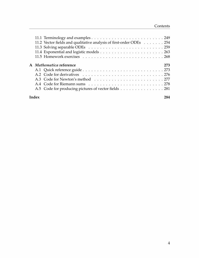
11.1 Terminology and examples . . . . . . . . . . . . . . . . . . . . . . . . . 24911.2 Vector fields and qualitative analysis of first-order ODEs . . . . . . . 25411.3 Solving separable ODEs . . . . . . . . . . . . . . . . . . . . . . . . . . 25911.4 Exponential and logistic models . . . . . . . . . . . . . . . . . . . . . . 26311.5 Homework exercises . . . . . . . . . . . . . . . . . . . . . . . . . . . . 268
A Mathematica reference 273A.1 Quick reference guide . . . . . . . . . . . . . . . . . . . . . . . . . . . . 273A.2 Code for derivatives . . . . . . . . . . . . . . . . . . . . . . . . . . . . 276A.3 Code for Newton’s method . . . . . . . . . . . . . . . . . . . . . . . . 277A.4 Code for Riemann sums . . . . . . . . . . . . . . . . . . . . . . . . . . 278A.5 Code for producing pictures of vector fields . . . . . . . . . . . . . . . 281
Index 284
4

Chapter 1
Algebra / Precalculus Review
1.1 Exponent and logarithm rulesExponent rules
Here is a list of exponent rules you should be familiar with. In calculus, we usethese exponent rules to rewrite a given expression in a way that makes it easier toperform calculus operations on the expression.
Theorem 1.1 (Exponent rules I) Let x, a, b and n be numbers, where x 6= 0. Then:
• xaxb = xa+b
• xa
xb= xa−b
• x0 = 1
• x−a = 1xa
• (xa)b = xab
• n√x = x1/n (in particular,
√x = x1/2)
• xm/n = n√xm = ( n
√x)m (this last way of writing xm/n is most useful)
Example: Simplify each expression as much as possible and write the answerso that it has no radical signs (i.e. no √ or 3
√ , etc.) or fractions with xs in thedenominators:
1. 642/3
Solution: 642/3 =(
3√
64)2
= 42 = 16.
5

1.1. Exponent and logarithm rules
2. 2−3
Solution: 2−3 = 123 = 1
8 .
3. 4−5/2
Solution: 4−5/2 = 145/2 = 1
(√
4)5 = 125 = 1
32 .
4. 3x4x−2(x3)3
Solution: 3x4x−2(x3)3 = 3x4x−2x9 = 3x4−2+9 = 3x11.
5. 1x7
Solution: 1x7 = x−7
6. 2x2
x4
Solution: 2x2
x4 = 2x2−4 = 2x−2
7.√x
Solution:√x = x1/2
8. 4√x7
Solution: 4√x7 = 4
x7/2 = 4x−7/2
Remark on existence of square roots:√x DNE if x < 0, and
√x means only
the nonnegative square root of x, i.e.√
25 = 5, not ±5. This is so that the processof taking a square root is a function (later).
Remark on simplifying square roots: For any positive number x,
(√x)2
= x.
But, if you do the square root and the squaring in the other order, the operationsdon’t cancel: √
x2 =
In general, if n is even then n√xn = |x|, but if n is odd, then n
√xn = x.
6

1.1. Exponent and logarithm rules
Theorem 1.2 (Exponent rules II) Let x, a, b and n be numbers, where x 6= 0. Then:
• (xy)a = xaya
•(xy
)a= xa
ya
Example: Simplify each expression as much as possible, and write the answerso that it has no radical signs or fractions with xs in the denominators:
1.(x3
)−3
Solution:(x3
)−3= x−3
3−3 = x−31
27= 27x−3.
2. x2√
x2
Solution: x2√
x2 = x2
√x√2 = x2 x1/2
√2 = x2+1/2
√2 = x5/2
√2 .
3. (2x)3x4
(4x)2
Solution: (2x)3x4
(4x)2 = 23x3x4
42x2 = 8x7
16x2 = 12x
5.
4. x0 3√
2(2x)2
Solution: x0 3√
2(2x)2 = 1 3√
2(22)(x2) = 3√
8x2 = 3√
8 3√x2 = 2x2/3.
WARNING: In general,
(x+ y)a 6= xa + ya and (x− y)a 6= xa − ya
As a special case of this, when a = −1 we see that
1x+ y
6= 1x
+ 1y
andA
x+ y6= A
x+ A
y.
7

1.1. Exponent and logarithm rules
Logarithm rules
Logarithms are the “inverse” operation of exponentials:
Definition 1.3 Let y and b be positive numbers. To say that x is the logarithm baseb of y means that by = x, i.e.
x = logb y ⇐⇒ bx = y.
The common logarithm of y is the logarithm base 10 of y, i.e.
x = log y ⇐⇒ 10x = y.
Euler’s constant is an irrational number denoted by e. It is approximately 2.7182818...The natural logarithm of y is the logarithm base e of y, i.e.
x = ln y ⇐⇒ ex = y.
(Logarithms of non-positive numbers are not defined.)
The reason why we care about the number e and natural logarithms has to dowith calculus: it turns out that calculus operations are “easier” when dealing withnatural exponentials and logarithms rather than exponentials and logarithms withbases other than e.
Notation: ex is also written exp(x), so exp(3x2 + y) means e3x2+y, etc.
Example: Evaluate the following expressions:
1. log 10000Solution: 104 = 10000, so log 10000 = log10 10000 = 4.
2. log3127
Solution: 3−3 = 133 = 1
27 , so log3127 = −3.
3. log6 36Solution: 62 = 36 so log6 36 = 2.
4. log4 32Solution: We know 32 = 4 · 4 · 2 = 4 · 4 · 41/2 = 41+1+1/2 = 45/2 so log4 32 = 5
2 .
5. ln e9
Solution: ln e9 = 9.
8
1.1. Exponent and logarithm rules
As with exponent rules, it is often convenient to rewrite expressions with loga-rithms in them before doing calculus:
Theorem 1.4 (Logarithm Rules) Let b, C and D be positive numbers, and let n beany number. Then:
• logb(CD) = logbC + logbD
• logb(CD
)= logbC − logbD
• logb 1 = 0
• logb(
1D
)= − logbD
• logb(Cn) = n logbC
• blogb C = C
• logb bC = C
Example: Use properties of logarithms to expand each logarithmic expressionas much as possible:
1. ln a5
b2
Solution: ln a5
b2 = ln a5 − ln b2 = 5 ln a− 2 ln b
2. log3√
5rSolution: log3
√5r = log3(5r)1/2 = 1
2 log3(5r) = 12 log3 5 + 1
2 log3 r
Example: Suppose x = log2 A, y = log2 B and z = log2 C. Find the following, interms of x, y and z:
1. log2 AB2
2. log28CA√B
3. 8A
Example: Write each of these expressions as the logarithm of a single quantity:
1. log x+ log ySolution: log x+ log y = log(xy)
9
1.1. Exponent and logarithm rules
2. 3 log x− 12 log y
Solution: 3 log x− 12 log y = log x3 − log y1/2 = log x3
y1/2
The world’s most underrated exponent rule allows you to write an arbitraryexponent as an exponent with base e:
Theorem 1.5 (Change of base formula for exponents) Let A and B be numberswith A > 0. Then:
AB = eB lnA.
Example: Rewrite the following expressions as a single exponent, so that thebase of the exponent is e:
1. e3exe−2y
Solution: e3exe−2y = e3+x−2y.
2. (e2x)4e−3x
Solution: (e2x)4e−3x = e2x·4e−3x = e8xe−3x = e8x−3x = e5x.
3. 53x
Solution: 53x = e3x ln 5 by the preceding Theorem.
4. e2x4x
Solution: e2x4x = e2xex ln 4 = e(2+ln 4)x.
A similar rule allows you to write an arbitrary logarithm in terms of naturallogarithms:
Theorem 1.6 (Change of base formula for logarithms) Let B and C be positivenumbers. Then:
logB C = lnClnB.
Example: Rewrite the following expressions in terms of natural logarithms:
1. log x
2. 4 log3(4x)
Example: Suppose x = lnA and y = lnB. What is logAB in terms of x and y?
Solution: logAB = lnBlnA = y
x.
10
1.2. Functions
Example: Solve the following equations for x:
1. e3x − 4 = 0
2. log3(4x− 1) = 2
1.2 FunctionsQuestion: What is a function?
11

1.2. Functions
Definition 1.7 Let A and B be sets. A function f from A to B is
We denote such a function by writing “f : A → B”. The set A of inputs is called thedomain of f . The set of outputs of the function is called the range of f .
In Math 220, we study functions where:
• the domain is R, the set of real numbers (sometimes the domain is a subsetof R like an interval), and
• the outputs are also real numbers.
Such a function f is often denoted by the symbols “f : R→ R”.
Example: Let f be the function R → R which takes the input, squares it, andthen adds 3 to produce the output.
To describe this function f , we could take some example inputs and see whatthe outputs are, arranging the results in a table:
INPUT OUTPUT
-2
-1
0
1
2
12
1.2. Functions
Rather than continuing to list inputs and outputs like this, it is easier to take ageneric input (something we call x and figure out what the generic output is. Thisoutput is called f(x). Writing down a formula for f(x) in terms of x is sufficient todescribe any function f : R→ R; such a formula is called a “rule” for the function.
In the example on the previous page, we can therefore describe the function bywriting
f(x) = x2 + 3.
Definition 1.8 Let f : A → B and let x ∈ A. We write the output associated toinput x as f(x); this is pronounced “f of x”. A formula for f(x) in terms of x iscalled a rule for the function.
Notation:
f (x)
Idea: Think of the x as a placeholder which represents where the input goes.Given a rule for f , you take whatever input you are given and replace all the xs inthe rule with that input.
Example: Let f(x) = 2x2 +x. Compute and simplify the following expressions:
1. f(2) = 2 · 22 + 2 = 2 · 4 + 2 = 10.
2. f(−1)
3. f(x) + f(3)
4. f(trumpet)
5. f(hamburger) = 2(hamburger)2 + hamburger
6. f(2x)
7. f(x− 1)
8. f(x)− f(1)
13

1.2. Functions
9. f(x+ h)
10. f(x+3)−f(x)3
WARNING: All your life you have been told that parenthesis means multipli-cation, i.e. 3(2) = 6 or a(b + c) = ab + ac. The parenthesis in the definition off(x) do not mean multiplication. In particular, f(x) does not mean f times x, andf(a+ b) is not the same thing as f(a) + f(b) (in general). f(x) means:
“the output of function f when x is the input”.
and is better denoted by the diagram
xf−→ f(x)
The graph of a function f : R→ REarlier, we saw the following table of values for the function whose rule is f(x) =x2 + 3:
INPUT OUTPUTx f(x)
-2 7
-1 4
0 3
1 4
2 7
-2 -1 1 2
1
2
3
4
5
6
7
14
1.2. Functions
Turning each of the inputs and outputs to the function into an ordered pair andplotting all these points produces a picture called the graph of the function. Notethat since every input has at most one output, functions from R to R must pass theVertical Line Test (i.e. every vertical line must hit the graph in at most one point).
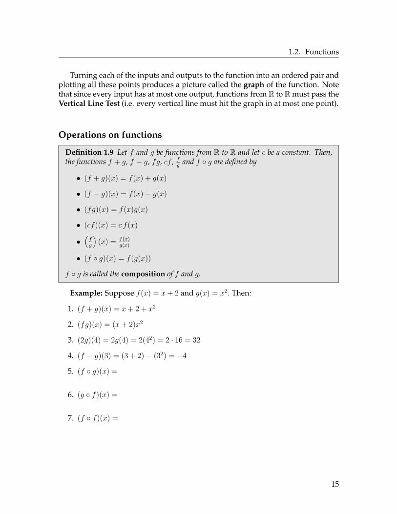
Operations on functions
Definition 1.9 Let f and g be functions from R to R and let c be a constant. Then,the functions f + g, f − g, fg, cf , f
gand f ◦ g are defined by
• (f + g)(x) = f(x) + g(x)
• (f − g)(x) = f(x)− g(x)
• (fg)(x) = f(x)g(x)
• (cf)(x) = c f(x)
•(fg
)(x) = f(x)
g(x)
• (f ◦ g)(x) = f(g(x))
f ◦ g is called the composition of f and g.
Example: Suppose f(x) = x+ 2 and g(x) = x2. Then:
1. (f + g)(x) = x+ 2 + x2
2. (fg)(x) = (x+ 2)x2
3. (2g)(4) = 2g(4) = 2(42) = 2 · 16 = 32
4. (f − g)(3) = (3 + 2)− (32) = −4
5. (f ◦ g)(x) =
6. (g ◦ f)(x) =
7. (f ◦ f)(x) =
15
1.2. Functions
Example: Given each function F , write F = f ◦ g where f and g are “easy”functions:
1. F (x) = (3x− 2)12
Solution: f(x) = x12; g(x) = 3x− 2
2. F (x) = ln7 x
3. F (x) = ln x7
4. F (x) = 5 cos(ex + 2x− 1)
5. F (x) = e−x
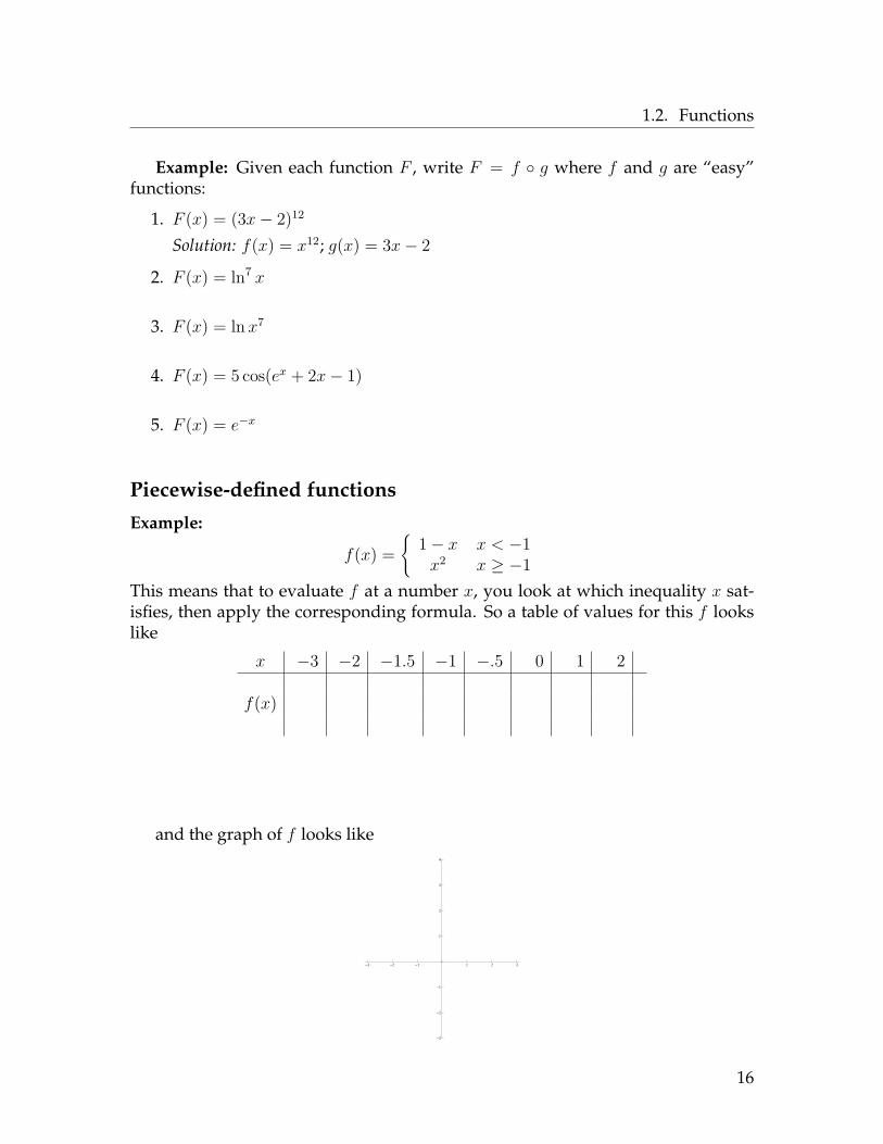
Piecewise-defined functions
Example:
f(x) ={
1− x x < −1x2 x ≥ −1
This means that to evaluate f at a number x, you look at which inequality x sat-isfies, then apply the corresponding formula. So a table of values for this f lookslike
x −3 −2 −1.5 −1 −.5 0 1 2
f(x)
and the graph of f looks like
-3 -2 -1 1 2 3
-3
-2
-1
1
2
3
4
16

1.2. Functions
Example:
f(x) ={x2 x 6= 2−1 x = 2
-5 -4 -3 -2 -1 1 2 3 4 5
-2
-1
1
2
3
4
5
6
Common functions whose graphs you should know
f(x) = x f(x) = x2 f(x) = x3
-3 -2 -1 1 2 3
-3
-2
-1
1
2
3
-3 -2 -1 1 2 3
-3
-2
-1
1
2
3
-3 -2 -1 1 2 3
-3
-2
-1
1
2
3
f(x) = 1x
f(x) = |x| f(x) = ex
-3 -2 -1 1 2 3
-3
-2
-1
1
2
3
-3 -2 -1 1 2 3
-3
-2
-1
1
2
3
1
1
e
f(x) = ln x f(x) = sin x f(x) = cos x
1 e
1
-2 Π -3 Π
2-Π -
Π
2
Π
2Π
3 Π
22 Π
-1
1
-2 Π -3 Π
2-Π -
Π
2
Π
2Π
3 Π
22 Π
-1
1
17

1.3. Lines
Transformations on functions
It is useful to know how the graph of a function changes if you alter the rule of thefunction a little bit. Suppose you know the graph of function f . Then:
Altered version of function f(all cs are positive numbers) Corresponding transformation on the graph
f(x) + c graph shifts up c units
f(x)− c graph shifts down c units
f(x+ c) graph shifts left c units
f(x− c) graph shifts right c units
cf(x) graph stretched vertically by factor of c(taller if c > 1, shorter if 0 < c < 1)
f(−x) graph reflected through y-axis
−f(x) graph reflected through x-axis
1.3 LinesBy far the most important class of functions are lines. Reasons:
1. Linear equations model a large class of real-world problems
2. Linear equations are relatively easy to work with.
3. You can often approximate the solution to hard problems (using calculustechniques) by considering something related to a linear equation.
18
1.3. Lines
Question: What “determines” a line? That is, what makes one line differentfrom another one?
1.
2.
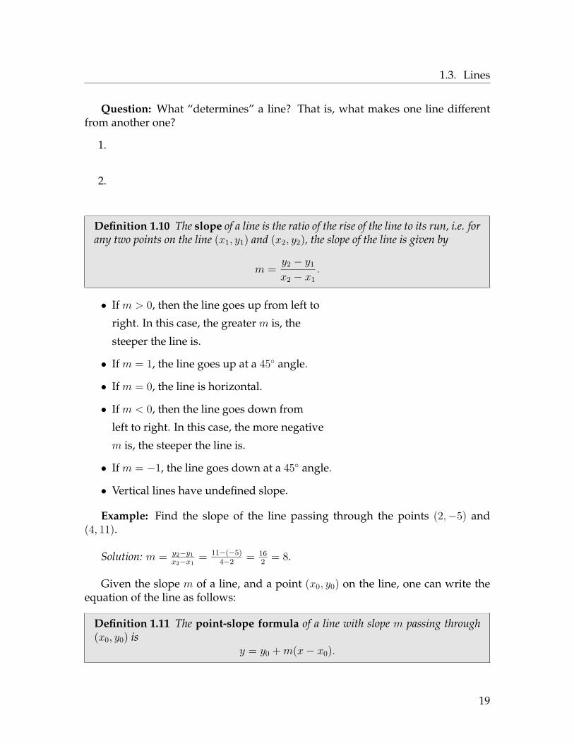
Definition 1.10 The slope of a line is the ratio of the rise of the line to its run, i.e. forany two points on the line (x1, y1) and (x2, y2), the slope of the line is given by
m = y2 − y1
x2 − x1.
• If m > 0, then the line goes up from left to
right. In this case, the greater m is, the
steeper the line is.
• If m = 1, the line goes up at a 45◦ angle.
• If m = 0, the line is horizontal.
• If m < 0, then the line goes down from
left to right. In this case, the more negative
m is, the steeper the line is.
• If m = −1, the line goes down at a 45◦ angle.
• Vertical lines have undefined slope.
Example: Find the slope of the line passing through the points (2,−5) and(4, 11).
Solution: m = y2−y1x2−x1
= 11−(−5)4−2 = 16
2 = 8.
Given the slope m of a line, and a point (x0, y0) on the line, one can write theequation of the line as follows:
Definition 1.11 The point-slope formula of a line with slope m passing through(x0, y0) is
y = y0 +m(x− x0).
19

1.3. Lines
You may be familiar with the “slope-intercept” formula y = mx + b for a line.The point-slope formula
y = y0 +m(x− x0)
is equivalent, because it can be rewritten as
It is extremely useful to know the point-slope formula, because it is easierthan the y = mx+ b formula to apply in calculus.
Example: Write the equation of the line passing through (2,−5) and (6,−7).
Example: Write the equation of the line passing through (−3,−2) with slope 25 .
NOTE: Vertical lines do not have a slope, so their equation cannot be writtenusing the point-slope formula. The equation of a vertical line is x = h, where h is aconstant. For example, the vertical line passing through (6,−5) is x = 6.
20
1.4. Trigonometry
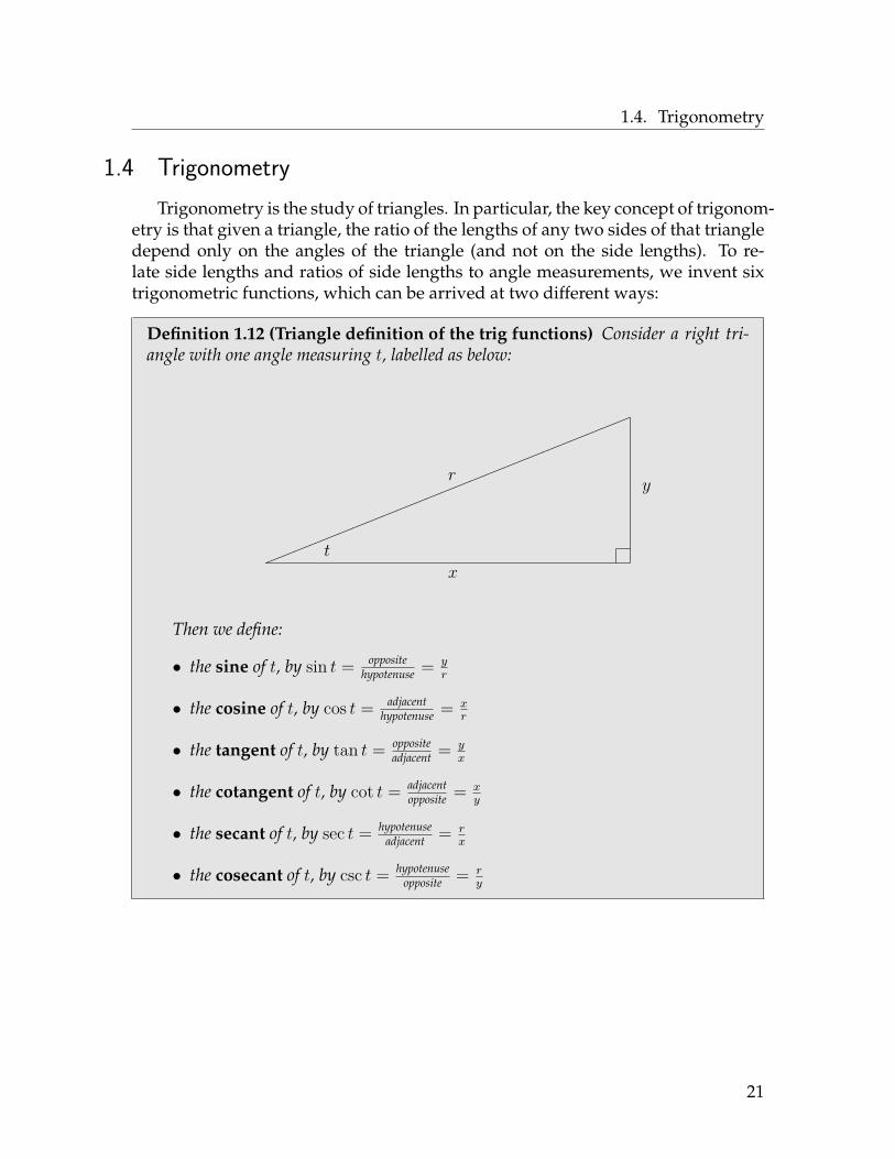
1.4 TrigonometryTrigonometry is the study of triangles. In particular, the key concept of trigonom-
etry is that given a triangle, the ratio of the lengths of any two sides of that triangledepend only on the angles of the triangle (and not on the side lengths). To re-late side lengths and ratios of side lengths to angle measurements, we invent sixtrigonometric functions, which can be arrived at two different ways:
Definition 1.12 (Triangle definition of the trig functions) Consider a right tri-angle with one angle measuring t, labelled as below:
!!!!
!!!!
!!!!
!!!!
!!!!
!!!!
!
x
yr
t
Then we define:
• the sine of t, by sin t = oppositehypotenuse = y
r
• the cosine of t, by cos t = adjacenthypotenuse = x
r
• the tangent of t, by tan t = oppositeadjacent = y
x
• the cotangent of t, by cot t = adjacentopposite = x
y
• the secant of t, by sec t = hypotenuseadjacent = r
x
• the cosecant of t, by csc t = hypotenuseopposite = r
y
21
1.4. Trigonometry
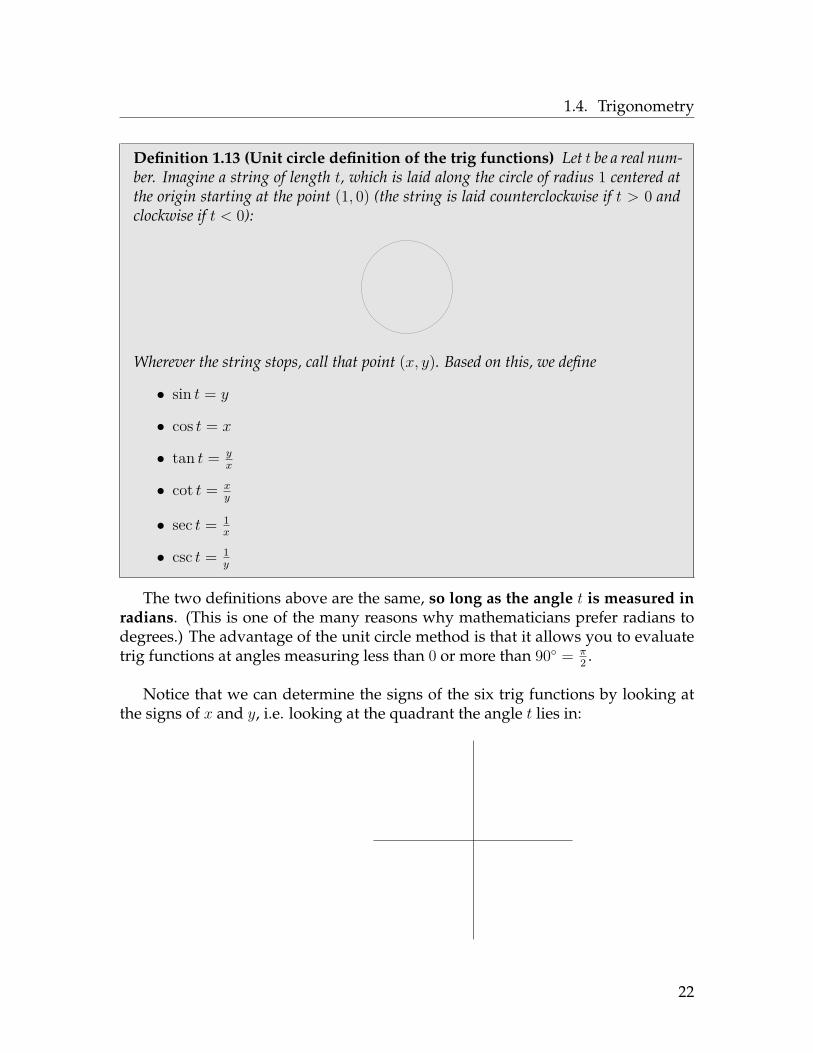
Definition 1.13 (Unit circle definition of the trig functions) Let t be a real num-ber. Imagine a string of length t, which is laid along the circle of radius 1 centered atthe origin starting at the point (1, 0) (the string is laid counterclockwise if t > 0 andclockwise if t < 0):
Wherever the string stops, call that point (x, y). Based on this, we define
• sin t = y
• cos t = x
• tan t = yx
• cot t = xy
• sec t = 1x
• csc t = 1y
The two definitions above are the same, so long as the angle t is measured inradians. (This is one of the many reasons why mathematicians prefer radians todegrees.) The advantage of the unit circle method is that it allows you to evaluatetrig functions at angles measuring less than 0 or more than 90◦ = π
2 .
Notice that we can determine the signs of the six trig functions by looking atthe signs of x and y, i.e. looking at the quadrant the angle t lies in:
22

1.4. Trigonometry
Either way you choose to define the trig functions, it is straightforward to de-duce the following relationships:
Theorem 1.14 (Trigonometric identites) Given the trig functions as defined above,the following identities hold for all x:
• Quotient identities:
1. tan x = sinxcosx
2. cotx = cosxsinx
• Reciprocal identities:
1. cotx = 1tanx
2. secx = 1cosx
3. cscx = 1sinx
• Pythagorean identities:
1. sin2 x+ cos2 x = 12. 1 + cot2 x = csc2 x
3. 1 + tan2 x = sec2 x
• Odd-even identities:
1. sin(−x) = − sin x2. cos(−x) = cos x3. tan(−x) = − tan x
Using these identities and the “All Scholars Take Calculus” rules, you can findthe values of all six trig functions if you are given the value of one trig function,and the sign of a second trig function:
Example: Find the values of all six trig functions of θ, if sin θ = 711 and tan θ < 0.
23
1.4. Trigonometry
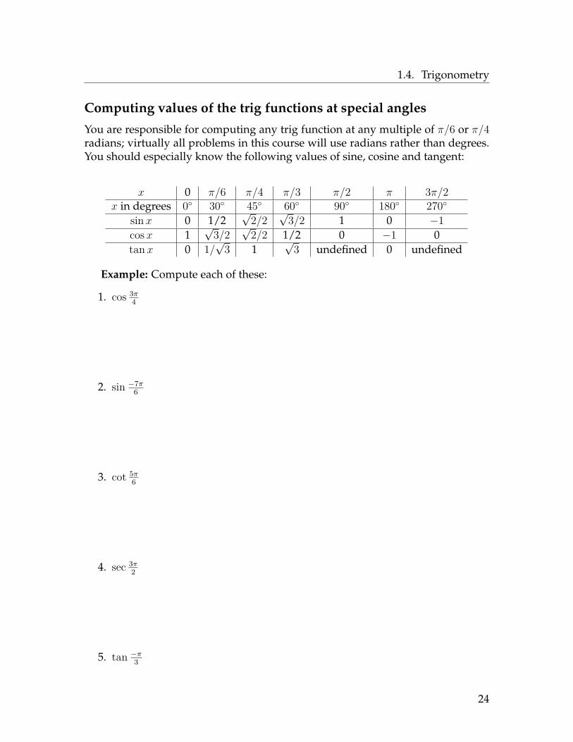
Computing values of the trig functions at special angles
You are responsible for computing any trig function at any multiple of π/6 or π/4radians; virtually all problems in this course will use radians rather than degrees.You should especially know the following values of sine, cosine and tangent:
x 0 π/6 π/4 π/3 π/2 π 3π/2x in degrees 0◦ 30◦ 45◦ 60◦ 90◦ 180◦ 270◦
sin x 0 1/2√
2/2√
3/2 1 0 −1cosx 1
√3/2
√2/2 1/2 0 −1 0
tan x 0 1/√
3 1√
3 undefined 0 undefined
Example: Compute each of these:
1. cos 3π4
2. sin −7π6
3. cot 5π6
4. sec 3π2
5. tan −π3
24

1.4. Trigonometry
Inverse trigonometric functions
It will be convenient to have notation for inverses of two of the trigonometric func-tions:
Definition 1.15 The arctangent (a.k.a. inverse tangent) function is the functionarctan : R→ R defined by
arctan x = an angle (in radians) between−π2 and
π
2 , whose tangent is x.
The arcsine (a.k.a. inverse sine) function is the function arcsin : [−1, 1] → Rdefined by
arcsin x = an angle (in radians) between−π2 and
π
2 , whose sine is x.
Example: arctan 1 = π4 because tan π
4 = 1.
Example: arcsin√
32 = π
3 because sin π3 =
√3
2 .
Notation: arctan x is sometimes written as tan−1 x, and arcsin x is sometimeswritten as sin−1 x.
Graphs of arctangent and arcsine:
f(x) = arctan x f(x) = arcsin x
-1 1
-Π
2
-Π
4
Π
4
Π
2
-1 1
-Π
2
-Π
4
Π
4
Π
2
Theorem 1.16 (Properties of arctangent and arcsin) These hold for all real num-bers x, y:
• arctan(−x) = − arctan x and arcsin(−x) = − arcsin x.
• y = arctan x ⇐⇒ x = tan y
• y = arcsin x ⇐⇒ x = sin y
25
1.5. Homework exercises
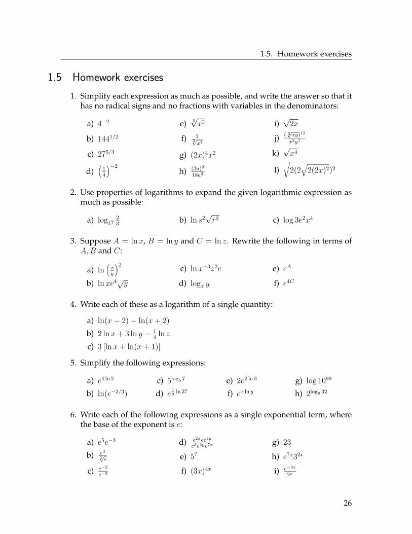
1.5 Homework exercises1. Simplify each expression as much as possible, and write the answer so that it
has no radical signs and no fractions with variables in the denominators:
a) 4−2
b) 1441/2
c) 275/3
d)(
14
)−2
e) 5√x3
f) 13√x4
g) (2x)4x2
h) (3a)2
18a3
i)√
2x
j) ( 3√xy)12
x3y7
k)√x4
l)√
2(2√
2(2x)2)2
2. Use properties of logarithms to expand the given logarithmic expression asmuch as possible:
a) log1723 b) ln s2
√r3 c) log 3e2x4
3. Suppose A = ln x, B = ln y and C = ln z. Rewrite the following in terms ofA,B and C:
a) ln(xy
)2
b) ln xe4√y
c) ln x−3z2e
d) logx y
e) eA
f) e4C
4. Write each of these as a logarithm of a single quantity:
a) ln(x− 2)− ln(x+ 2)b) 2 ln x+ 3 ln y − 1
4 ln zc) 3 [ln x+ ln(x+ 1)]
5. Simplify the following expressions:
a) e4 ln 2
b) ln(e−2/3)c) 5log5 7
d) e13 ln 27
e) 2e2 ln 3
f) ex ln y
g) log 1099
h) 2log8 32
6. Write each of the following expressions as a single exponential term, wherethe base of the exponent is e:
a) e5e−3
b) e33√e
c) e−2
e−5
d) e2xee4y
e3e2ye7x
e) 57
f) (3x)4x
g) 23
h) e7x32x
i) e−3x
2x
26
1.5. Homework exercises
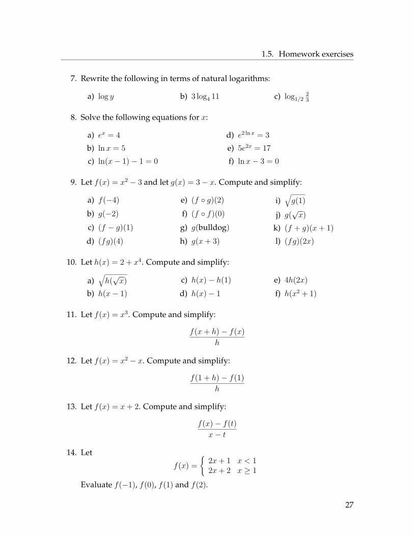
7. Rewrite the following in terms of natural logarithms:
a) log y b) 3 log4 11 c) log1/223
8. Solve the following equations for x:
a) ex = 4b) ln x = 5c) ln(x− 1)− 1 = 0
d) e2 lnx = 3e) 5e2x = 17f) ln x− 3 = 0
9. Let f(x) = x2 − 3 and let g(x) = 3− x. Compute and simplify:
a) f(−4)b) g(−2)c) (f − g)(1)d) (fg)(4)
e) (f ◦ g)(2)f) (f ◦ f)(0)g) g(bulldog)h) g(x+ 3)
i)√g(1)
j) g(√x)
k) (f + g)(x+ 1)l) (fg)(2x)
10. Let h(x) = 2 + x4. Compute and simplify:
a)√h(√x)
b) h(x− 1)c) h(x)− h(1)d) h(x)− 1
e) 4h(2x)f) h(x2 + 1)
11. Let f(x) = x3. Compute and simplify:
f(x+ h)− f(x)h
12. Let f(x) = x2 − x. Compute and simplify:
f(1 + h)− f(1)h
13. Let f(x) = x+ 2. Compute and simplify:
f(x)− f(t)x− t
14. Let
f(x) ={
2x+ 1 x < 12x+ 2 x ≥ 1
Evaluate f(−1), f(0), f(1) and f(2).
27

1.5. Homework exercises
15. Sketch the graph of the function
f(x) ={
1− x x < 1x+ 1 x ≥ 1
16. Sketch the graph of the function
f(x) ={
x x 6= 1−1 x = 1
17. Given the graphs below (where f is the solid line and g is the dashed line):
-4 -2 2 4
-4
-2
2
4
a) Find f(−2)b) Find g(3).
c) Find g(−3).
d) Find (f + g)(−1).
e) Find (f ◦ g)(3).
f) Find (fg)(1).
g) Find all value(s) x (if any) such that f(x) = g(x).
h) Find all value(s) x (if any) for which f(x) = −1.
i) Find all value(s) x (if any) for which g(x) = 0.
28

1.5. Homework exercises
18. Suppose the graph below is the picture of a function where the output ofthe function is a company’s profit (in millions of dollars), and the input isthe price at which the company sells its product. At (roughly) what priceshould the company sell its product, if its goal is to make as much money aspossible? How much profit will be made at this price?
0 5 10 15 20 25 30 35 40 45 50 55 60 65 70 75 80 85 90 95 100
5
10
15
20
25
30
35
40
45
50
55
60
65
70
75
80
85
90
95
100
19. Determine which one or ones of the following pictures (a)-(d) depict situa-tions where y is a function of x.
a)
-4 -2 2 4
-4
-2
2
4
b)
-4 -2 2 4
-4
-2
2
4
c)
-4 -2 2 4
-4
-2
2
4
d)
-4 -2 2 4
-4
-2
2
4
20. Suppose y = f(x) is a function whose graph is:
-3 -2 -1 1 2 3
-2
-1
1
2
Sketch the graphs of the following functions:
a) y = f(x+ 5)b) y = f(x)− 5
c) y = f(−x)d) y = −f(x) + 5
e) y = f(x− 2) + 1f) y = −f(−x)
29

1.5. Homework exercises
21. Sketch the graphs of the following functions:
a) y = 2 sin xb) y = (x− 3)2 + 1c) y = − ln x
d) y = e−x
e) y = cos(−x)f) y = −(x+ 2)3
g) y = −|x|+ 2h) y = − 1
x
i) y = −(x+ 2)2 − 4
22. Estimate the slope of each of the following lines by looking at its graph:
a)
-4 -2 2 4
-4
-2
2
4
b)
-4 -2 2 4
-4
-2
2
4
c)
-4 -2 2 4
-4
-2
2
4
d)
-4 -2 2 4
-4
-2
2
4
e)
-4 -2 2 4
-4
-2
2
4
23. Find the slope of the line passing through these pairs of points:
a) (3,−4) and (5, 2)b) (−1
2 ,23) and (−3
4 ,16)
c) (a, b) and (a+ s, b+ r)
d) (2, 7) and (2,−1)e) (x, f(x)) and (x+ h, f(x+ h))f) (−1, 4) and (5,−8)
24. Find the equation of the line with each set of properties:
a) passes through (0, 3) and has slope 34
b) passes through the origin; m = 23
c) passes through (2, 1) and (0,−3)d) passes through (−3,−2); m = 4e) passes through (2, 6) and is vertical
f) passes through (−4, 2) and is horizontal
g) passes through (5, 1) and (5, 8)h) passes through (−7, 3) and (2,−5)
25. Suppose sin x = 513 . Assuming the values of the other five trig functions of x
are positive, find them.
26. Suppose cosx = 725 . If tan x < 0, find the values of the other five trig functions
of x.
27. Suppose cscx = 52 . What is sin x?
28. Suppose tan x = 2. If cosx < 0, what is sin x?
30
1.5. Homework exercises
29. Compute each of the following (if they are not defined, say so). Try to dothese without looking anything up (to simulate how you will have to do thesethings on quizzes and exams).
a) sin π3
b) cos π2
c) tan π4
d) cos 0e) cos π
6
f) cos 2π3
g) sin 3π2
h) cot 3π4
i) sin 0j) sec π
k) tan π6
l) sin 7π4
m) sec π3
n) tan 3π2
o) sin π
p) csc 5π6
q) sec −π4r) sin −5π
6
s) tan−πt) tan −8π
3
30. Evaluate each of the following:
a) arcsin 12
b) arcsin 0
c) arctan 1
d) arctan(−√
3)
e) arctan√
33
f) arcsin −√
32
g) arcsin−1h) arctan−1
i) arcsin −√
22
Answers
DISCLAIMER: Throughout the lecture notes, the provided answers are answersonly (not complete solutions) and may contain errors and/or typos.
1. a) 116
b) 12c) 243d) 16
e) x3/5
f) x−4/3
g) 16x6
h) 12a−1
i) 21/2x1/2
j) xy−3
k) x2
l) 8|x|
2. a) log17 2− log17 3b) 2 ln s+ 3
2 ln rc) log 3 + 2 log e+ 4 log x
3. a) 2A− 2Bb) A+ 4 + 1
2B
c) −3A+ 2C + 1d) B
A
e) x
f) z4
4. a) ln(x−2x+2
)b) ln (x2y3 4
√z) c) ln [x(x+ 1)]3
5. a) 16b) −2
3
c) 7d) 3
e) 18f) yx
g) 99h) 25/3
31

1.5. Homework exercises
6. a) e2
b) e8/3
c) e3
d) e−5x+2y−2
e) e7 ln 5
f) e4x ln(3x)
g) eln 23
h) e7x+2x ln 3
i) e−3x−x ln 2
7. a) ln yln 10 b) 3 ln 11
ln 4 c) ln(2/3)ln(1/2) = ln 2−ln 3
− ln 2
8. a) x = ln 4b) x = e5
c) x = e+ 1
d) x =√
3e) x = 1
2 ln 175
f) x = e3
9. a) 13b) −1c) −4d) −13
e) −2f) 6g) 3− bulldog
h) x
i)√
2j) 3−
√x
k) (x+ 1)2 − x− 1l) (4x2 − 3)(3− 2x)
10. a)√
2 + x2
b) 2 + (x− 1)4
c) x4 − 1d) x4 + 1
e) 8 + 64x4
f) 2 + (x2 + 1)4
11. 3x2 + 3xh+ h2
12. h+ 1
13. 1
14. f(−1) = −1; f(0) = 1; f(1) = 4; f(2) = 6.
15.
-3 -2 -1 1 2 3
-1
1
2
3
16.
-2 -1 1 2
-2
-1
1
2
32

1.5. Homework exercises
17. a) 3b) 0c) DNE
d) 4e) 1f) 4
g) x = 1h) x = −4, x = −2i) x = 3
18. The price should be roughly $45, and their profit will be about $92, 000, 000.
19. (a) and (d) are functions.
20. a)
-7 -6 -5 -4 -3 -2 -1 1 2 3
-2
-1
1
2
b)
-3 -2 -1 1 2 3
-6
-5
-4
-3
-2
-1
1
c)
-3 -2 -1 1 2 3
-2
-1
1
2
d)-3 -2 -1 1 2 3
-1
1
2
3
4
5
6
7
e)-1 1 2 3 4 5
-1
1
2
3
f)
-3 -2 -1 1
-2
-1
1
2
21. a)-6 -5 -4 -3 -2 -1 1 2 3 4 5 6
-3
-2
-1
1
2
3
b) -1 1 2 3 4 5 6
-1
1
2
3
4
5
6
c)
-1 1 2 3 4 5 6
-3
-2
-1
1
2
3
d)-3 -2 -1 1 2 3 4
-1
1
2
3
4
5
e)-6 -5 -4 -3 -2 -1 1 2 3 4 5 6
-3
-2
-1
1
2
3
f)
-5 -4 -3 -2 -1 1
-3
-2
-1
1
2
3
g)
-3 -2 -1 1 2 3
-2
-1
1
2
3
33

1.5. Homework exercises
h)
-3 -2 -1 1 2 3
-3
-2
-1
1
2
3
i)
-5 -4 -3 -2 -1 1
-8
-7
-6
-5
-4
-3
-2
-1
1
22. a) 0 b) ≈ 13 c) ≈ −1 d) DNE e) ≈ 4
23. a) 3b) 2
c) rs
d) DNE
e) f(x+h)−f(x)h
f) −2
24. a) y = 34x+ 3
b) y = 23x
c) y = 2x− 3d) y = −2 + 4(x+ 3)
e) x = 2f) y = 2g) x = 5h) y = −5 + −8
9 (x− 2)
25. cosx = 1213 ; tan x = 5
12 ; cotx = 125 ; secx = 13
12 ; cscx = 135 .
26. sin x = −2425 ; tan x = −24
7 ; cotx = −724 ; secx = 25
7 ; cscx = −2524 .
27. 25
28. −1√5
29. a)√
32
b) 0c) 1d) 1
e)√
32
f) −12
g) −1h) −1
i) 0j) −1
k)√
33
l) −√
22
m) 2n) DNE
o) 0p) 2
q)√
2r) −1
2
s) 0t)√
3
30. a) π6
b) 0c) π
2
d) −π3e) π
6
f) −π3
g) −π2h) −π4i) −π4
34

Chapter 2
Limits
2.1 The idea of the limitWarmup: Given the graphs of each of these functions, tell me the value of f(2):
(1)
-1 1 2 3 4
-1
1
2
3
4
(3)
-1 1 2 3 4
-1
1
2
3
4
(2)
-1 1 2 3 4
-1
1
2
3
4
Answers:
(1)
(2)
(3)
35

2.1. The idea of the limit
Modified warmup: Here is the graph of some function f . The portion of thegraph above x = 2 is “covered” (by a strip of tape, for example). Based only onwhat you see, what would you guess the value of f(2) is?
-1 1 2 3 4
-1
1
2
3
4
First idea of the limit: graphical interpretation
Suppose you can see the entire graph of a function f except for the possible pointon the graph sitting above (or below) x = a. If, based on the picture, you’d guessthat f(a) = L, then you say
“the limit as x approaches a of f(x) is L”
and you’d write
limx→a
f(x) = L or “f(x)→ L as x→ a′′.
Examples: In the modified warmup above,
limx→2
f(x) =
In all three warmup examples,limx→2
f(x) =
Note: f(2) is different in the three warmup examples. In one example, f(2) doesn’teven exist!
36

2.1. The idea of the limit
In general, if you have a function f which satisfies
limx→a
f(x) = L,
then the graph of f should look like one of these three pictures:
Back to the modified warmup:
-1 1 2 3 4
-1
1
2
3
4
In this example, we said limx→2
f(x) = 1.Why was 1 the most reasonable guess for the value of f(2)?
Second idea of the limit: approximation via tables
To saylimx→a
f(x) = L
means that as x gets closer and closer to a (without ever reaching a), the corre-sponding values f(x) of the function get closer and closer to L.
37
2.1. The idea of the limit
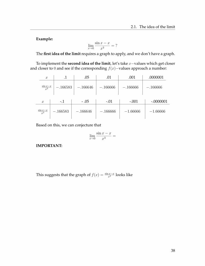
Example:
limx→0
sin x− xx3 = ?
The first idea of the limit requires a graph to apply, and we don’t have a graph.
To implement the second idea of the limit, let’s take x−values which get closerand closer to 0 and see if the corresponding f(x)−values approach a number:
x .1 .05 .01 .001 .0000001
sinx−xx3 −.166583 −.166646 −.166666 −.166666 −.166666
x -.1 - .05 -.01 -.001 -.0000001
sinx−xx3 −.166583 −.166646 −.166666 −1.66666 −1.66666
Based on this, we can conjecture that
limx→0
sin x− xx3 =
IMPORTANT:
This suggests that the graph of f(x) = sinx−xx3 looks like
38

2.1. The idea of the limit
The method of the previous example sometimes works well, but it can lie:
Example: f(x) = cos 1x.
limx→0
f(x) = ?
Here’s a graph of f(x):
1
10 Π
1
8 Π
1
7 Π
1
6 Π
1
5 Π
1
4 Π
1
3 Π
1
2 Π
-1
1
Let’s try the method of the previous example:
x 12π
14π
16π
1100π
11000π
f(x)
x 13π
15π
17π
1101π
11001π
f(x)
39

2.2. One-sided limits
Third idea of the limit: formal definition
Suppose f(x) is defined for all x near a but possibly not at a. If f(x) is as close to Las we like for all x sufficiently close to a (but not a itself), we say
limx→a
f(x) = L.
In the previous example,
2.2 One-sided limitsExample: Let
f(x) = |x|x
={
1 if x > 0−1 if x < 0 .
limx→0
f(x) = ?
-3 -2 -1 1 2 3
-2
-1
1
2
40

2.2. One-sided limits
Definition 2.1 Suppose f(x) is defined for all x near a with x > a. If (whenever xgets closer and closer to a from the right, f(x) approaches L), then we say the limit off(x) as x approaches a from the right is L and we write
limx→a+
f(x) = L.
Suppose f(x) is defined for all x near a with x < a. If (whenever x gets closer andcloser to a from the left, f(x) approaches L), then we say the limit of f(x) as xapproaches a from the left is L and we write
limx→a−
f(x) = L.
These are also called, respectively, left-hand limits and right-hand limits. Collec-tively, left- and right-hand limits are referred to as one-sided limits.
Example: In the previous example where f(x) = |x|x
,
limx→0+
f(x) = limx→0−
f(x) =
Theorem 2.2 limx→a
f(x) exists only if limx→a+
f(x) and limx→a−
f(x) both exist and areequal. In this situation,
limx→a
f(x) = limx→a+
f(x) = limx→a−
f(x).
Example: For the function f(x) = |x|x
, since
limx→0+
f(x) = 1 6= −1 = limx→0−
f(x),
we see thatlimx→0
f(x) DNE.
41

2.2. One-sided limits
Example: Consider the following graph of some unknown function f :
-7 -6 -5 -4 -3 -2 -1 1 2 3 4 5 6 7
-4
-3
-2
-1
1
2
3
4
5
6
Based on this graph, find the following:
1. limx→2
f(x)
2. limx→0
f(x)
3. f(2)
4. f(0)
5. limx→2+
f(x)
6. limx→−3−
f(x)
7. limx→−3+
f(x)
8. limx→−3
f(x)
9. f(4)
10. limx→4+
f(x)
11. limx→4−
f(x)
12. limx→4
f(x)
42

2.3. Infinite limits
2.3 Infinite limitsConsider the function f(x) = 1
x. What happens to f(x) as x→ 0?
x 1 .5 .1 .001 .0000001
f(x) 1 2 10 1000 1000000
x -1 - .5 -.1 -.001 -.0000001
f(x) −1 −2 −10 −1000 −1000000
-4 -2 2 4
-4
-2
2
4
We invent new notation to describe this situation. We say
limx→0+
1x
=∞ and limx→0−
1x
= −∞.
43

2.3. Infinite limits
Formally:
• to say limx→a+
f(x) =∞means that as x gets closer and closer to a from the right,
the numbers f(x) grow without bound.
• to say limx→a+
f(x) = −∞ means that as x gets closer and closer to a from the
right, the numbers f(x) become more and more negative without bound.
• to say limx→a−
f(x) =∞means that as x gets closer and closer to a from the left,
the numbers f(x) grow without bound.
• to say limx→a−
f(x) = −∞ means that as x gets closer and closer to a from the
left, the numbers f(x) become more and more negative without bound.
All these situations are called infinite limits. The graphical description of aninfinite limit is as follows:
44

2.4. Limits at infinity
Definition 2.3 If limx→a+
f(x) = ±∞ or limx→a−
f(x) = ±∞, we say the vertical line
x = a is a vertical asymptote (VA) for f(x).
Example: x = 0 is a VA for f(x) = 1x.
NOTE: ∞ is not a number. It is only a symbol. However, in the context oflimits,∞ can be manipulated in some ways as if it was a number (we’ll see how inChapter 3). For now you should remember these facts:
limx→0+
1x
=∞ limx→0−
1x
= −∞
One infinite limit to memorize:
limx→0+
ln x = −∞
1 e
1
Other infinite limits are computed using techniques we will study later, to-gether with the rules of arithmetic with∞ described above.
2.4 Limits at infinityWe want to consider the values of f(x) when x gets larger and larger without
bound.
Example: f(x) = 1x.
x 1 10 10000 10100 1010000
f(x) 1 110
110000
110100
11010000
45

2.4. Limits at infinity
We say limx→∞
f(x) = L if
• (heuristically) when x grows without bound, f(x) approaches L.• (graphically) the graph of f looks like
or
We say limx→−∞
f(x) = L if
• (heuristically) when x becomes more and more negative without bound, f(x)approaches L.
• (graphically) the graph of f looks like
or
Definition 2.4 If limx→∞
f(x) = L or limx→−∞
f(x) = L, we say the horizontal line y = L
is a horizontal asymptote (HA) for f(x).
46

2.4. Limits at infinity
Example: Consider the following graph of some unknown function f :
-10 -9 -8 -7 -6 -5 -4 -3 -2 -1 1 2 3 4 5 6 7 8
-6
-5
-4
-3
-2
-1
1
2
3
4
5
6
7
8
Based on this graph, find the following:
1. limx→∞
f(x)
2. limx→−∞
f(x)
3. limx→−3+
f(x)
4. limx→−3−
f(x)
5. limx→−3
f(x)
6. limx→3+
f(x)
7. limx→3−
f(x)
8. limx→3
f(x)
9. the equation(s) of any vertical asymptote(s) of f
10. the equation(s) of any horizontal asymptote(s) of f
47

2.5. Homework exercises
2.5 Homework exercisesIn Problems 1-2 below, use a calculator or computer to complete the tables and
use the results to estimate the value of the limit:
1.limx→3
x− 3x2 − 7x+ 12
x 2.9 2.99 2.999f(x)x 3.1 3.01 3.001
f(x)
2.
limx→−2
√2− x− 2x+ 2
x -2.1 -2.01 -2.001f(x)x -1.9 -1.99 -1.999
f(x)
3. Find the value of the following limit using tables similar to Problems 1 and2. (This time, you have to pick your own x values.)
limx→0
ln(x+ 1)− xx2
4. Find the value of the following limit using tables similar to Problems 1 and2. (Again, you have to pick your own x values.)
limx→1
1− 2x+1
x− 1
5. Complete the following charts for the function f(x) = |x−5|x−5 :
x 5.1 5.01 5.001f(x)x 4.9 4.99 4.999
f(x)
What do these charts suggest to you about limx→5
|x−5|x−5 ?
48

2.5. Homework exercises
6. Given the graph of f below, evaluate the given expressions. If the quantitydoes not exist, say so.
-8 -7 -6 -5 -4 -3 -2 -1 1 2 3 4 5 6 7 8
-6
-5
-4
-3
-2
-1
1
2
3
4
5
6
a) limx→−5
f(x)
b) f(−5)c) lim
x→−1f(x)
d) limx→1−
f(x)
e) limx→1+
f(x)
f) limx→1
f(x)
g) limx→4−
f(x)
h) limx→4+
f(x)
i) limx→4
f(x)
j) f(4)
7. Given the graph of g below, evaluate the given expressions. If the quantitydoes not exist, say so.
-10 -9 -8 -7 -6 -5 -4 -3 -2 -1 1 2 3 4 5 6 7 8 9 10
-8
-7
-6
-5
-4
-3
-2
-1
1
2
3
4
a) limx→−8
g(x)
b) f(−8)c) lim
x→−5g(x)
d) limx→0−
g(x)
e) limx→1
g(x)
f) limx→7−
g(x)
g) limx→7+
g(x)
h) limx→7
g(x)i) g(7)j) lim
x→−2−g(x)
49

2.5. Homework exercises
8. Sketch a graph of a function f which has all of the following four properties(there are many possible correct answers):
• f(0) is not defined;• limx→0 f(x) = 4;• f(2) = 6;• limx→2 f(x) = 3.
9. Sketch a graph of a function f which has all of the following five properties(there are many possible correct answers):
• limx→−1+ f(x) = 3;• limx→−1− f(x) = −2;• limx→2− f(x) DNE;• f(2) = 0;• limx→2+ f(x) = 3.
In Problems 10-11 below, complete the tables (use a calculator or computer ifnecessary) and use the results to estimate the value of the limit:
10.limx→∞
4x+ 32x− 1
x 10 100 1000 106 1010
f(x)
11.limx→∞
−6x√4x2 + 5
x 10 100 1000 106 1010
f(x)
In Problems 12-17 below, graph the function inside the limit using Mathematica(or a calculator) and use the graph of the function to estimate lim
x→∞f(x):
12. f(x) = |x|x+1
13. f(x) = lnx√x
14. f(x) = sinxx
15. f(x) = x arctan(
1x
)16. f(x) = x−
√x(x− 1)
17. f(x) = x+1x√x
50

2.5. Homework exercises
In Problems 18-19 below, complete the tables (use a calculator or computer ifnecessary) and use the results to estimate the value of the limit:
18.limx→1+
2 + x
1− x
x 2 1.1 1.01 1.0001 1.000001f(x)
19.
limx→3−
x2 + 7x− 3
x 2 2.9 2.99 2.9999 2.999999f(x)
In Problems 20-25 below, graph the function inside the limit using Mathematica anduse the graph of the function to estimate the given limit:
20. limx→π−
sec(x2 )
21. limx→π+
sec(x2 )
22. limx→0
(x−1)2
x2
23. limx→π−
(cotx− secx)
24. limx→4−
3x2−6x+5x2−5x+4
25. limx→1−
x−4ex−e
26. Find the equation of any horizontal and/or vertical asymptotes of the func-tion
f(x) = x2 + 3x3 − 5x2 + 4x.
27. Find the equation of any horizontal and/or vertical asymptotes of the func-tion
f(x) = 2x2 − 8x− 42x2 − 25 .
28. Find the equation of any horizontal and/or vertical asymptotes of the func-tion
f(x) = (x− 3)(x+ 4)(x− 7)x(x− 3)(x+ 1) .
51

2.5. Homework exercises
29. Given the graph of f below, evaluate the given limits.
-10 -9 -8 -7 -6 -5 -4 -3 -2 -1 1 2 3 4 5 6 7 8 9 10
-10-9-8-7-6-5-4-3-2-1
123456789
10
a) limx→∞
f(x)
b) limx→−∞
f(x)
c) limx→−5−
f(x)
d) limx→−5+
f(x)
e) limx→−5
f(x)
f) limx→1+
f(x)
g) limx→1−
f(x)
h) limx→1
f(x)
30. Given the graph of g below, evaluate the given limits.
-5 -4 -3 -2 -1 1 2 3 4 5 6 7 8 9 10
-3
-2
-1
1
2
3
4
5
6
7
a) limx→∞
g(x)
b) limx→−∞
g(x)
c) limx→2−
g(x)
d) limx→2+
g(x)
e) limx→2
g(x)
f) limx→5+
g(x)
g) limx→5−
g(x)
h) limx→5
g(x)
52
2.5. Homework exercises
Answers
1. limx→3
x−3x2−7x+12 = −1
2. limx→−2
√2−x−2x+2 = −1
4
3. −12
4. 12
5. limx→5
|x−5|x−5 DNE (left-
and right-hand lim-its are unequal)
6. a) 1b) −3c) −1d) 1e) DNE
f) DNE
g) 5h) 1i) DNE
j) 1
7. a) −4b) 2c) −2d) 3e) about −1f) about 1.5g) −3
h) DNE
i) DNE
j) −5
8. Many answers arepossible.
9. Many answers arepossible.
10. limx→∞
4x+32x−1 = 2
11. limx→∞
−6x√4x2+5 = −3
12. 1
13. 0
14. 0
15. 1
16. 12
17. 0
18. limx→1+
2+x1−x = −∞
19. limx→3−
x2+7x−3 = −∞
20. ∞
21. −∞
22. ∞
23. −∞
24. −∞
25. ∞
26. HA: y = 0VA: x = 0, x = 1, x =4.
27. HA: y = 2VA: x = 5, x = −5.
28. HA: y = 1VA: x = 0, x = −1.
29. a) 3b) −2c) −∞d) ∞e) DNE
f) −∞g) −∞h) −∞
30. a) ∞b) 1c) ∞d) ∞e) ∞f) ∞g) −∞h) DNE
53
Chapter 3
Computing Limits
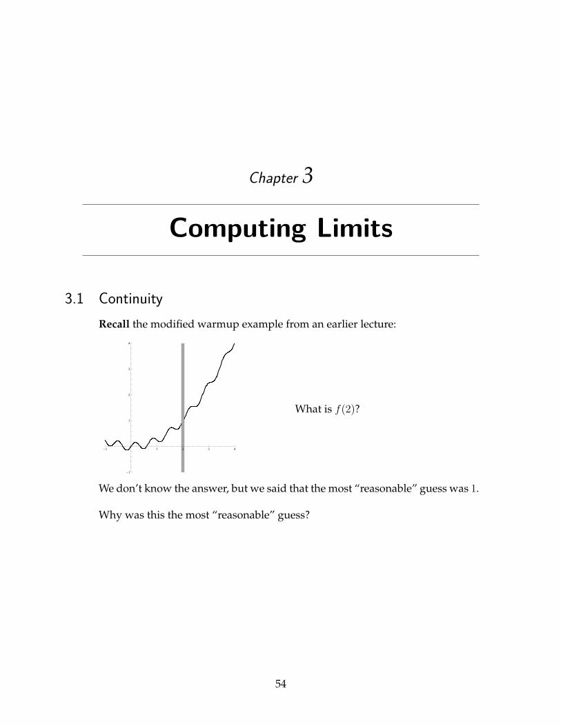
3.1 ContinuityRecall the modified warmup example from an earlier lecture:
-1 1 2 3 4
-1
1
2
3
4
What is f(2)?
We don’t know the answer, but we said that the most “reasonable” guess was 1.
Why was this the most “reasonable” guess?
54

3.1. Continuity
Mathematically, this is described by the notion of “continuity”. For example:
Functions whose graphs have no breaks are called “continuous”. More pre-cisely:
Definition 3.1 A function f is called continuous at the point x = a if
1. f(a) exists;
2. limx→a
f(x) exists (i.e. limx→a+
f(x) = limx→a−
f(x)); and
3. limx→a
f(x) = f(a) (i.e. limx→a+
f(x) = limx→a−
f(x) = f(c)).
Otherwise we say f is discontinuous at x = a.
The word continuous is abbreviated “cts”.
Classification of discontinuities
1. If limx→a
f(x) exists but either f(a) DNE or f(a) 6= limx→a
f(x), we say f has a re-movable discontinuity (a.k.a. hole discontinuity) at a:
55

3.1. Continuity
2. If limx→a−
f(x) and limx→a+
f(x) both exist but are not equal, then we say f has a
jump discontinuity at a.
3. If limx→a+
f(x) or limx→a−
f(x) = ±∞, we say f has an infinite discontinuity at a.
4. If limx→a+
f(x) or limx→a−
f(x) DNE because of too many wiggles, we say f has an
oscillating discontinuity at a.
Example: Given the following graph of some unknown function f , determinethe places where f is discontinuous; and classify the type of discontinuity at eachof these points:
-3 -2 -1 1 2 3 4 5 6 7
-1
1
2
3
4
56

3.1. Continuity
Definition 3.2 A function f is called continuous on an interval if it is continuousat every point in that interval. A function f is called continuous if it is continuousat every point in its domain.
Dictionary of continuous functions
The following functions are continuous, because there are no breaks in their graphs:
Theorem 3.3 Suppose f and g are continuous functions. Then:
1. f + g, f − g, fg, and f ◦ g are continuous; and
2. fg
is continuous at all x where g(x) 6= 0.
Theorem 3.4 Any function made up of powers of x, sines and cosines, arcsines, arct-angents, exponentials and/or logarithms using addition, subtraction, and/or multipli-cation is continuous (at every point of its domain).
Theorem 3.5 Any function which is the quotient of functions made up of powers ofx, sines, cosines, arcsines, arctangents, exponentials and/or logarithms is continuouseverywhere except where the denominator is zero.
57

3.2. Evaluation of limits
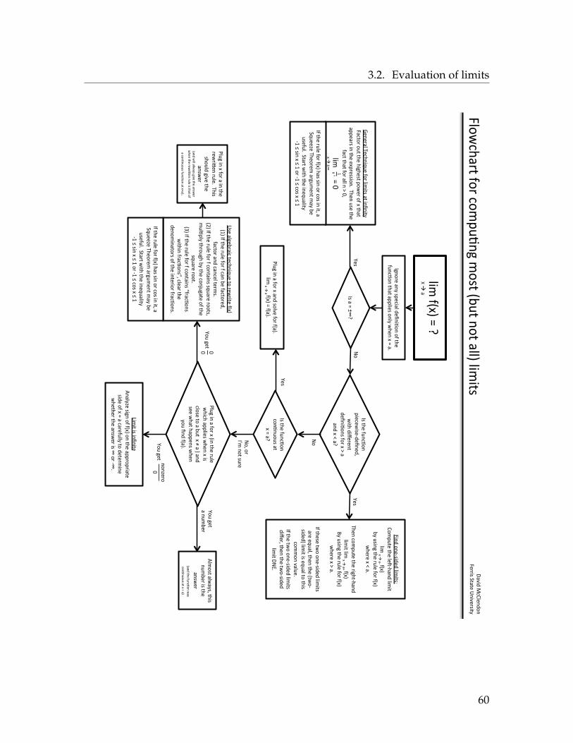
3.2 Evaluation of limitsFor the most part, one should use the flowchart on page 60 to evaluate limits.
However, it is good to keep in mind the following concepts:
First concept: limits behave “nicely” with respect to arithmetic
Theorem 3.6 (Main Limit Theorem) Suppose limx→a
f(x) and limx→a
g(x) both exist andare finite, where a is either ±∞ or a finite number. Then:
1. limx→a
[f(x) + g(x)] = limx→a
f(x) + limx→a
g(x);
2. limx→a
[f(x)− g(x)] = limx→a
f(x)− limx→a
g(x);
3. limx→a
[k f(x)] = k · limx→a
f(x) for any constant k;
4. limx→a
[f(x)g(x)] =[limx→a
f(x)] [
limx→a
g(x)];
5. limx→a
[f(x)g(x)
]=
limx→a
f(x)
limx→a
g(x) provided the denominator is nonzero.
6. limx→a
n
√f(x) = n
√limx→a
f(x) provided both sides exist.
7. limx→a
ef(x) = exp(
limx→a
f(x))
.
8. limx→a
ln f(x) = ln(
limx→a
f(x))
.
Second concept: evaluate limits of cts functions by plugging in
If f is continuous at a, then limx→a
f(x) = f(a).
Third concept: ignore f(a) in general
f(a) has nothing to do with the value of limx→a
f(x).
The second and third concepts seem contradictory, but aren’t.
Fourth concept: manipulate expressions with∞ using rules
Although ∞ is not a number, it can be mainpulated in some ways as if it is anumber. (See the next page for details.)
58
3.2. Evaluation of limits
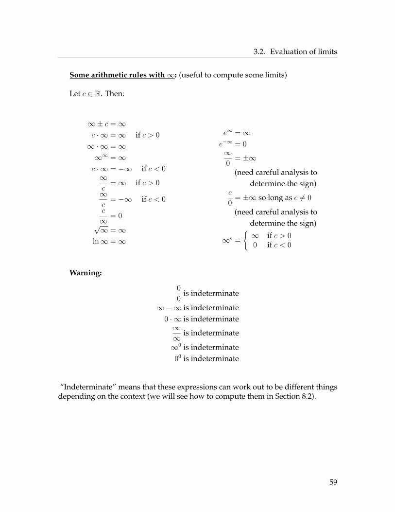
Some arithmetic rules with∞: (useful to compute some limits)
Let c ∈ R. Then:
∞± c =∞c · ∞ =∞ if c > 0∞ ·∞ =∞∞∞ =∞c · ∞ = −∞ if c < 0∞c
=∞ if c > 0∞c
= −∞ if c < 0c
∞= 0
√∞ =∞
ln∞ =∞
e∞ =∞e−∞ = 0∞0 = ±∞
(need careful analysis todetermine the sign)
c
0 = ±∞ so long as c 6= 0
(need careful analysis todetermine the sign)
∞c ={∞ if c > 00 if c < 0
Warning:
00 is indeterminate
∞−∞ is indeterminate0 · ∞ is indeterminate∞∞
is indeterminate
∞0 is indeterminate00 is indeterminate
“Indeterminate” means that these expressions can work out to be different thingsdepending on the context (we will see how to compute them in Section 8.2).
59
3.2. Evaluation of limits
!"#$%&'($)
$*$
$+$!
$,$
-./012$,/3$45
26",
!$728/"90/$0%$:;
2$
%</690/$:;
,:$,
55!"24$0
/!3$=
;2/$'$)
$,>$
-4$,$)$?@*$
A24$
B2/21,!$C26;/"D<2$%0
1$!"#":4$,
:$"/8/":3$
E,6:0
1$0<:$:;
2$;".;
24:$5
0=21$0
%$'$:;,:$
,552,14$"/
$:;2$2'51244"0
/>$$C
;2/$<42$:;
2$
%,6:$:;
,:$%0
1$,!!$/
$F$GH$
!"#$$$$$$$)
$G$
'$!$?@$
I$
'$ /$
J0$
-4$:;2$%<
/690/$
5"262="42
K728/27H$
=":;
$7"L212/:$
728/"90/4$%0
1$'$F$,$
,/7$'$M
$,*$
A24$
E"/7$0/2K4"7
27$!"#
":4N$
O0#5<:2$:;
2$!2PK;,/7$!"#
":$$
!"#$'$!
$,K$ %&'($
Q3$<
4"/.$:;
2$1<
!2$%0
1$%&'($
=;212$'$M
$,>$
$
C;2/$60
#5<:2$:;
2$1".;
:K;,/7$
!"#":$!"#
$'$!$,R$ %&'($
S3$<
4"/.$:;
2$1<
!2$%0
1$%&'($
=;212$'$F
$,>$
$
-%$:;242$:=
0$0/2K4"7
27$!"#
":4$
,12$2D<,!H$:;
2/$:;
2$&:=
0K
4"727($!"#
":$"4$2D<,!$:0
$:;"4$
60##0/$T,
!<2>$
-%$:;2$:=
0$0/2K4"7
27$!"#
":4$
7"L21H$:;
2/$:;
2$:=
0K4"7
27$
!"#":$U
JV>$
J0$
-4$:;2$%<
/690/$
60/9/<0<4$,
:$
'$)$,*$J0H$01$
-W#$/0:$4<
12$
A24$
X!<.$"/
$,$%0
1$'$,/7$40
!T2$%0
1$%&,(>$
!"#$'$!
$,$ %&'($)
$%&,(>$
X!<.$"/
$,$%0
1$'$&"/$:;
2$1<
!2$
=;"6;
$,55!"24$=
;2/$'$"4$
6!042$:0
$,$Q<:$$'$Y
$,$($,
/7$
422$=;,:$;
,552/4$=
;2/$
30<$8/7$%&,
(>$
A0<$.2
:$$ G$
G$
Z42$,!.2
Q1,"6$:2
6;/"D<2$:0
$12=1":2
$%&'($
&I($-%$:;
2$1<
!2$%0
1$%$6,/$Q2$%,6:0
127H$
%,6:0
1$,/7$6,
/62!$:2
1#4>$$$
&[($-%$:;
2$1<
!2$%0
1$%$60/:,"/4$4D
<,12$10
0:4H$
#<!95!3$:;
10<.;$Q3$:;
2$60
/\<.,:2$0%$:;
2$
4D<,12$10
0:>$
&]($-%$:;
2$1<
!2$%0
1$%$60/:,"/4$^%1,
690/4$
=":;
"/$%1,
690/4_H$6!2
,1$:;
2$
72/0#"/,:014$0
%$:;2$"/:21"0
1$%1,690/4>$
X!<.$"/
$'$%01$,
$"/$:;
2$
12=1"`
2/$1<
!2>$$C
;"4$
4;0<!7$."T2
$:;2$
,/4=
21$$
&,/7$="!!$,
!=,34$."T2
$:;2$,/4=
21$
=;2/$:;
2$12
=1"`
2/$1<
!2$"4$:;
,:$0
%$
,$60
/9/<0<4$%<
/690/$,:$')
,(>$
A0<$.2
:$$
,$/<#Q21$$
a!#
04:$,
!=,34H$:;
"4$
/<#Q21$"4$:;
2$
,/4=
21$
$&,/7$:;
2$%<
/690/$=,4$
60/9/<0<4$,
:$'$)$,($
-%$:;2$1<
!2$%0
1$%&'($;,4$4"/
$01$60
4$"/$":H$,
$
bD<22c2$C;2012#$,1.<
#2/:$#
,3$Q
2$
<42%<!>$$b:,
1:$=":;
$:;2$"/2D<,!":3$$
KI$d$4"/
$'$d$I$01$KI
$d$60
4$'$d$I$
-%$:;2$1<
!2$%0
1$%&'($;,4$4"/
$01$60
4$"/$":H$,
$
bD<22c2$C;2012#$,1.<
#2/:$#
,3$Q
2$
<42%<!>$$b:,
1:$=":;
$:;2$"/2D<,!":3$$
KI$d$4"/
$'$d$I$01$KI
$d$60
4$'$d$I$
A0<$.2
:$$ /0/c210$
G$
e"#":$"4$"/
8/":2
$
a/,!3c2
$4"./$0%$%&'($0
/$:;
2$,551051",
:2$
4"72$0%$'$)
$,$6,
12%<!!3$:0
$72:21#
"/2$
=;2:;21$:;
2$,/4=
21$"4$@
$01$K@
>$
E!0=6;,1:$%0
1$60#5<9/.$#
04:$&Q
<:$/
0:$,
!!($!"#":4$
U,T"7
$f6O!2/70/$
E211"4$b:,
:2$Z/"T2
14":3$
60

3.2. Evaluation of limits
Evaluating limits at infinity
Example 1
limx→∞
4 + 3x2
8x2 + 3x+ 2
Example 1 could have been phrased differently: suppose you were asked to findthe horizontal asymptotes of f(x) = 4+3x2
8x2+3x+2 .
Example 2
limx→∞
x√2x2 + 1
61

3.2. Evaluation of limits
Example 3
limx→∞
−3− 5x2
2x4 − x+ 52
Example 4
limx→∞
2x2 + 7x− 2x− 1
62
3.2. Evaluation of limits
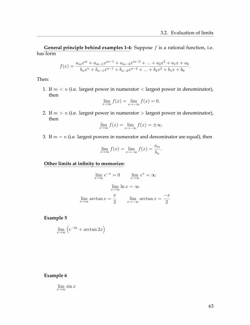
General principle behind examples 1-4: Suppose f is a rational function, i.e.has form
f(x) = amxm + am−1x
m−1 + am−2xm−2 + ...+ a2x
2 + a1x+ a0
bnxn + bn−1xn−1 + bn−2xn−2 + ...+ b2x2 + b1x+ b0.
Then:
1. If m < n (i.e. largest power in numerator < largest power in denominator),then
limx→∞
f(x) = limx→−∞
f(x) = 0.
2. If m > n (i.e. largest power in numerator > largest power in denominator),then
limx→∞
f(x) = limx→−∞
f(x) = ±∞.
3. If m = n (i.e. largest powers in numerator and denominator are equal), then
limx→∞
f(x) = limx→−∞
f(x) = ambn.
Other limits at infinity to memorize:
limx→∞
e−x = 0 limx→∞
ex =∞
limx→∞
ln x =∞
limx→∞
arctan x = π
2 limx→−∞
arctan x = −π2
Example 5
limx→∞
(e−3x + arctan 2x
)
Example 6
limx→∞
sin x
63

3.2. Evaluation of limits
Evaluation of limits of piecewise-defined functions
Example 7
limx→2
f(x) where f(x) =
x2 − 2 x < 2
5 x = 2x+ 3 x > 2
Example 8
limx→2
f(x) where f(x) ={x2 − 1 x < 2x+ 1 x ≥ 2
64

3.2. Evaluation of limits
Evaluation of limits of continuous functions
Key fact: If f is continuous at a, then limx→a
f(x) = f(a).
Example 9
limx→3
x2 + 3x− 1
Example 10limx→π
2
3 cos 2x
Example 11limx→0
e2x
65

3.2. Evaluation of limits
Evaluation of limits of functions which are not known to becontinuous
Given limit limx→a
f(x), start by plugging in a to the function f .
1. if you get a number when you plug in, almost always this is the answer (andthe function is actually continuous at a);
2. if you get nonzero0 , the limit is infinite; carefully analyze the sign of f(x) to
determine whether the answer is∞ or −∞;
3. if you get 00 , use an algebraic technique to rewrite f :
a) if f can be factored, factor and cancel terms;b) if f contains square roots which are added or subtracted, multiply through
by the conjugate (then factor and cancel);c) if f contains “fractions within fractions”, clear the denominators of the
interior fractions (then factor and cancel).
Example 12
limx→3+
(2
(x− 3)2 + 2x2)
Example 13
limx→2+
44− x2
66

3.2. Evaluation of limits
Example 14
limx→2−
44− x2
Example 15
limx→2
44− x2
Example 16
limx→3
x2 + 2x− 15x2 − 7x+ 12
67

3.2. Evaluation of limits
Example 17
limx→−1
√x2 + 8− 3x+ 1
Example 18
limt→4
√t− 2
2t− 8
68

3.2. Evaluation of limits
Example 19
limx→−1
1x
+ 11
x+2 − 1
69

3.2. Evaluation of limits
Example 20
limx→0
x2 sin(1x
)
Theorem 3.7 (Squeeze Theorem) Suppose f(x) ≤ g(x) ≤ h(x). If
limx→a
f(x) = limx→a
h(x) = L,
then limx→a
g(x) = L as well.
A picture to explain:
Back to Example 20
The Squeeze Theorem is a useful “last-resort” technique for evaluating limitswith sines and cosines in it, since−1 ≤ sin(anything) ≤ 1 and−1 ≤ cos(anything) ≤1.
70

3.3. Homework exercises
3.3 Homework exercisesIn Problems 1-9, discuss the continuity of each function (that means list the
values x at which the function is not continuous, and for each of these x, classifythe discontinuity as “removable”, “jump”, “infinite”, or “oscillating”. (If necessary,use Mathematica to obtain a graph of the function.)
1. The function whose graph is
-8 -7 -6 -5 -4 -3 -2 -1 1 2 3 4 5 6 7 8
-6
-5
-4
-3
-2
-1
1
2
3
4
5
6
2. The function whose graph is
-5 -4 -3 -2 -1 1 2 3 4 5 6 7 8 9 10
-3
-2
-1
1
2
3
4
5
6
7
3. f(x) = −3x−3
4. f(x) = 1x2+1
5. f(x) = cos(πx)
6. f(x) = cos(x−2) + 2
7. f(x) = xx2−x
8. f(x) ={
x x ≤ 1x2 x > 1
9. f(x) ={
1− x x ≤ 1x2 x > 1
71

3.3. Homework exercises
In Problems 10-57, evaluate the given limit (algebraically, by hand). If the limitdoes not exist, say so.
10. limx→∞
x2+3x3−2
11. limx→∞
x2+3x2−2
12. limx→∞
x2+3x−2
13. limx→∞
3−2x2+x4x(x−1)
14. limx→∞
√x
x+1
15. limx→∞
x+1√4x2−x
16. limx→−∞
7x3
x3+1
17. limx→∞
ln(4x+ 1)
18. limx→∞
8 arctan x2
19. limx→∞
4ex+x
20. limx→∞
e4x−5
21. limx→∞
e−x2
22. limx→∞
sin 3xx
23. limx→2−
x−3x−2
24. limx→5+
x2
x2−25
25. limx→−2+
x+3x2+x−2
26. limx→4
x+2(x−4)2
27. limx→0−
(x2 − 1
x
)28. lim
x→0+x+1ex−1
29. limx→0+
3sinx
30. limx→0−
3sinx
31. limx→4
x+2x−4
32. limx→3+
ln(x− 3)
33. limx→−2
(x2 − 4x)
34. limx→3
x+5x2−1
35. limx→0
e−x
36. limx→5
3√x+ 3
37. limx→π
tan(x3
)38. lim
x→−3sin πx
39. limx→e2
ln x2
40. limx→5+
xx2−5
41. limx→−1
arctan x
42. limx→3
1x− 1
3x+3
43. limx→2
f(x), where f(x) ={x+ 2 x < 2x2 x ≥ 2
44. limx→2
f(x), where f(x) =
2x− 1 x < 2
8 x = 2x2 − 1 x > 2
72

3.3. Homework exercises
45. limx→2
f(x), where f(x) ={x2 − 1 x ≤ 2x+ 4 x > 2
46. limx→2
f(x), where f(x) ={x2 − x+ 1 x ≤ 1x3 + 3 x > 1
47. limx→−2
x2−3x−10x2+5x+6
48. limx→4
x2−16x2+x−20
49. limx→1
x3−3x2+2xx−1
50. limx→0
√x+7−
√7
x
51. limx→1
1−x√x+3−2
52. limx→2
1x− 1
2x−2
53. limx→−1
2x−1 +1
1x
+1
54. limx→∞
sin 3xx
55. limx→0
x2 cos 2x
56. limx→0
x4 sin(x−2)
57. limx→0
cos 2x
Answers
1. x = −5 (removable)
x = 1 (infinite)
x = 3 (jump)
2. x = 0 (jump)
x = 2 (infinite)
x = 6 (oscillating)
3. x = 3 (infinite)
4. none
5. none
6. x = 0 (oscillating)
7. x = 0 (removable)
x = 1 (infinite)
8. none
9. x = 1 (jump)
10. 0
11. 1
73

3.3. Homework exercises
12. ∞
13. −12
14. 0
15. 12
16. 7
17. ∞
18. 4π
19. 0
20. ∞
21. 0
22. 0
23. ∞
24. ∞
25. −∞
26. ∞
27. ∞
28. ∞
29. ∞
30. −∞
31. DNE
32. −∞
33. 12
34. 1
35. 1
36. 2
37.√
3
38. −√
32
39. 4
40. 14
41. −π4
42. 0
43. 4
44. 3
45. DNE
46. 11
47. −7
48. 89
49. −1
50. 12√
7
51. −4
52. −14
53. 12
54. 0
55. 0
56. 0
57. DNE
74

Chapter 4
Introduction to Derivatives
4.1 Odometers and speedometersSuppose you get in your car and drive to Grand Rapids. There are two ways to
record your motion as a function of elapsed time t:
1.
2.
As an example, here are two graphs representing the same trip:
time t
odometer reading
time t
speedometer reading
Essentially, the content of Math 220 centers on the conversion from one of thesepictures to the other. In particular, we want to know:
1.
2.
75
4.1. Odometers and speedometers
In Chapters 4-8, we focus on the first question above and its other applications.We will turn to the second question in Chapter 9.
First major problem of calculus
Given a function f = f(t) which represents theposition of an object at time t, compute the object’s
instantaneous velocity at time t.
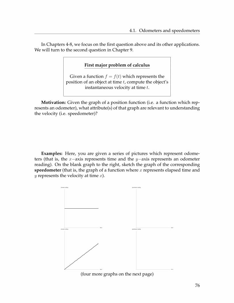
Motivation: Given the graph of a position function (i.e. a function which rep-resents an odometer), what attribute(s) of that graph are relevant to understandingthe velocity (i.e. speedometer)?
Examples: Here, you are given a series of pictures which represent odome-ters (that is, the x−axis represents time and the y−axis represents an odometerreading). On the blank graph to the right, sketch the graph of the correspondingspeedometer (that is, the graph of a function where x represents elapsed time andy represents the velocity at time x).
time t
odometer reading
time t
speedometer reading
time t
odometer reading
time t
speedometer reading
(four more graphs on the next page)
76

4.1. Odometers and speedometers
time t
odometer reading
time t
speedometer reading
time t
odometer reading
time t
speedometer reading
time t
odometer reading
time t
speedometer reading
time t
odometer reading
time t
speedometer reading
Punchline: Given a function f which measures distance traveled at time t, thecorresponding velocity at time t is the slope or steepness of the graph of f at time t.
But what is meant by “slope”? We know how to find the slope of a line (fromhigh-school algebra), but what is meant by the “slope” of a curve?
Idea:
Definition 4.1 Given a function f and a number x in the domain of f , the tangentline to f at x (if it exists) is the line which most closely approximates the graph of fat points very near x.
77

4.1. Odometers and speedometers
This definition implies a few things about tangent lines:
1.
2.
3.
Second major problem of calculus
Given a function f and a particular number x(sometimes I’ll use a for the value of x),
find (if possible) the slope of the line tangent to f at x.
Why do we care about finding the slope of a tangent line to a graph?
price
profit
(There will be other reasons coming later.)
Can we find the slope of a tangent line to a graph using just algebra?
78

4.2. Definition of the derivative
4.2 Definition of the derivativeLet’s try to find the slope of the line tangent to this function f at the indicated
point x:
79
4.2. Definition of the derivative
Back to the first major problem(find instantaneous velocity given position function)
Note: An object’s average velocity over some interval of time is given by
vavg = change in object’s positionelapsed time
.
Therefore if the object’s position at time t is given by f(t), then the object’s averagevelocity between times t1 and t2 is
v[t1,t2] =
So the object’s velocity over the time interval [x, x+ h] is
v[x,x+h] =
and its instantaneous velocity at time x is
80

4.2. Definition of the derivative
Notice that the formula
limh→0
f(x+ h)− f(x)h
solves both of the two major problems of calculus posed earlier in this chapter.This motivates the following definition:
Definition 4.2 (Limit definition of the derivative) Let f : R → R be a functionand let x be in the domain of f . If the limit
limh→0
f(x+ h)− f(x)h
exists and is finite, say that f is differentiable at x. In this case, we call the value ofthis limit the derivative of f and denote it by f ′(x) or df
dxor dy
dx.
The word “differentiable” is abbreviated “diffble”.
Some algebraic manipulation of the derivative formula:
Theorem 4.3 (Alternate limit definition of the derivative) Let f : R → R be afunction and let f be differentiable at x. Then
f ′(x) = limt→x
f(t)− f(x)t− x
.
Notation and verbiage:
• “derivative” is a noun. The verb form of this noun is “differentiate”, i.e. to“differentiate” a function means to compute the derivative of that function.
81

4.2. Definition of the derivative
• Given a function f and a particular value of x (say 4), the derivative of f atx = 4 is denoted
These are numbers.
• We can also think of the derivative as a function.
• Given an expression y = f(x), the derivative (thought of as a function) is alsodenoted
• The fractional notation with “d”s above is called Leibniz notation. In general,
d
dx(blah) = derivative of (blah)
At this point, we know that the derivative is used to compute the followingquantities:
1. f ′(x) gives the slope of the tangent line to f at the value x;
2. f ′(x) gives the slope of the curve f at the value x;
3. f ′(t) gives the instantaneous velocity of an object at time t, given that theobject’s position at time t is f(t);
4. f ′(x) gives the instantaneous rate of change of y = f(x) with respect to x.
Units: If y = f(x) is measured in some unit Uy and x is measured in some unitUx, then the units of f ′(x) are Uy/Ux. For example, if y is measured in lbs and x ismeasured in ft, then f ′(x) will be measured in lbs/ft.
82

4.2. Definition of the derivative
Question: What is the equation of the line tangent to differentiable function fat the point where x = a (a is a constant)?
Example 1 Use the definition of derivative to compute the slope of the linetangent to f(x) =
√x at the point (9, 3).
Example 2 Use the definition of derivative to compute the instantaneous ve-locity of an object at time 3, given that the object’s position at time t is given byf(t) = t2 − t.
83

4.2. Definition of the derivative
Example 3 Let f(x) = |x|. Find f ′(0).
Solution: Again, use the definition:
f ′(0) = limh→0
f(0 + h)− f(0)h
= limh→0
|h| − 0h
= limh→0
|h|h
What does it really mean for a function to be “differentiable” at x?
Theorem 4.4 (Differentiability implies continuity) Suppose f : R → R is dif-ferentiable at x. Then f must be continuous at x.
Theorem 4.5 A function f fails to be differentiable at x if:
1. f is not continuous at x; or
2. the tangent line to f at x is vertical; or
3. the graph of f has a corner or cusp at x.
84

4.2. Definition of the derivative
Example 4 Given below is the graph of some unknown function f :
-6 -5 -4 -3 -2 -1 1 2 3 4 5 6
-5
-4
-3
-2
-1
1
2
3
4
Use this graph to answer the questions below:
1. Give the values of x at which f is not continuous.
2. Give the values of x at which f is not differentiable.
3. Estimate f(1).
4. Estimate f ′(1).
5. Find two values of x for which f ′(x) = 0.
6. Estimate dfdx
∣∣∣x=5
Example 5 Compute the derivative f ′(0), given that
f(x) = (x+ 2)4√cosx.
85

4.3. Homework exercises
4.3 Homework exercisesIn these problems, you must compute all derivatives using the definition of the
derivative (do not use any “rules” you may know if you already took calculus).
1. Let f(x) = 4− 23x. Find f ′(x).
2. Find the derivative of f(x) = 1x+3 .
3. Compute dydx
if y =√
3x− 2.
4. Find the equation of the line tangent to the function f(x) = x3+1 when x = 1.
5. Find the slope of the line tangent to y =√x when x = 4.
6. Find the instantaneous velocity of an object at time 6, given that the object’sposition at time t is f(t) = 2t2 + 3t− 1.
7. Given the following graph of function f , give all the values x at which f isnot differentiable:
-10 -9 -8 -7 -6 -5 -4 -3 -2 -1 1 2 3 4 5 6 7 8 9 10
-6
-5
-4
-3
-2
-1
1
2
3
4
5
6
86

4.3. Homework exercises
8. Use the graph of the function f given below to answer the following ques-tions:
-10 -9 -8 -7 -6 -5 -4 -3 -2 -1 1 2 3 4 5 6 7 8 9 10 11 12
-4
-3
-2
-1
1
2
3
4
5
6
7
8
9
10
a) Estimate f(−6).
b) Estimate f ′(−6).
c) Estimate a value of x between −3 and 5 for which f ′(x) = 0.
d) Find all values of x at which f is not continuous.
e) Find all values of x at which f is not differentiable.
f) Estimate dfdx
∣∣∣x=−3
.
g) Is f ′(2) positive, negative or zero? Explain.
h) Estimate dydx
∣∣∣x=5
.
i) Estimate limx→∞ f(x).
j) Estimate limx→∞ f′(x).
k) Find the slope of the function f when x = −3.
l) Find the equation of the line tangent to f when x = −3.
m) Find the equation of the line tangent to f when x = 8.
n) On the graph above, sketch the graph of the tangent line to x when x =2.
87
4.3. Homework exercises
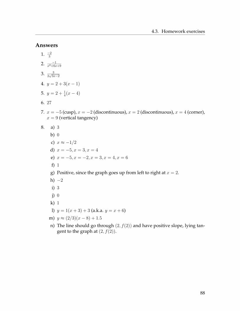
Answers
1. −23
2. −1x2+6x+9
3. 32√
3x−2
4. y = 2 + 3(x− 1)
5. y = 2 + 14(x− 4)
6. 27
7. x = −5 (cusp), x = −2 (discontinuous), x = 2 (discontinuous), x = 4 (corner),x = 9 (vertical tangency)
8. a) 3b) 0c) x ≈ −1/2d) x = −5, x = 3, x = 4e) x = −5, x = −2, x = 3, x = 4, x = 6f) 1g) Positive, since the graph goes up from left to right at x = 2.
h) −2i) 3j) 0
k) 1l) y = 1(x+ 3) + 3 (a.k.a. y = x+ 6)
m) y ≈ (2/3)(x− 8) + 1.5n) The line should go through (2, f(2)) and have positive slope, lying tan-
gent to the graph at (2, f(2)).
88

Chapter 5
Elementary DifferentiationRules
Recall: we want to figure out how to compute derivatives without using the limitdefinition.
General procedure for computing derivatives
1. Memorize the derivatives of a few basic functions(power, exponential, trigonometric, logarithmic, etc.)
2. Learn some rules which tell you how to compute the derivatives ofmore complicated functions in terms of the derivatives you havememorized.
Over the next two chapters we will develop these rules, which allow us to com-pute derivatives without having to resort to the limit definition.
89
5.1. Power rule
5.1 Power ruleExample: Find the derivative of f(x) = c, where c is a constant.Solution:
Theorem 5.1 (Constant Function Rule) Let c be a constant. Then ddx
(c) = 0.
Example: Find the derivative of f(x) = mx+ b, where m and b are constants.Solution:
f ′(x) = limh→0
f(x+ h)− f(x)h
= limh→0
[m(x+ h) + b]− [mx+ b]h
=
Theorem 5.2 (Linear Function Rule) If f(x) = mx+ b, then f ′(x) = m.
90
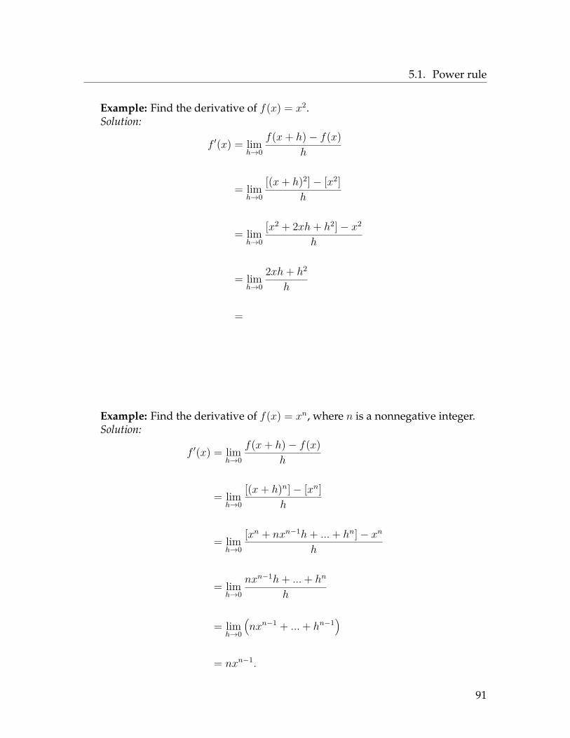
5.1. Power rule
Example: Find the derivative of f(x) = x2.Solution:
f ′(x) = limh→0
f(x+ h)− f(x)h
= limh→0
[(x+ h)2]− [x2]h
= limh→0
[x2 + 2xh+ h2]− x2
h
= limh→0
2xh+ h2
h
=
Example: Find the derivative of f(x) = xn, where n is a nonnegative integer.Solution:
f ′(x) = limh→0
f(x+ h)− f(x)h
= limh→0
[(x+ h)n]− [xn]h
= limh→0
[xn + nxn−1h+ ...+ hn]− xnh
= limh→0
nxn−1h+ ...+ hn
h
= limh→0
(nxn−1 + ...+ hn−1
)
= nxn−1.
91

5.1. Power rule
Example: Find the derivative of f(x) =√x.
Solution: Just to show you that you can use either definition of derivative, we’lldo this example with the alternate definition:
f ′(x) = limt→x
f(t)− f(x)t− x
= limt→x
√t−√x
t− x
= limt→x
(√t−√x)
(t− x) ·
(√t+√x)
(√t+√x)
= limt→x
t− x(t− x)
(√t+√x)
= limt→x
1√t+√x
= 1√x+√x
= 12√x.
Example: Find the derivative of f(x) = 1x.
Solution:
f ′(x) = limt→x
f(t)− f(x)t− x
= limt→x
1t− 1
x
t− x
=
92
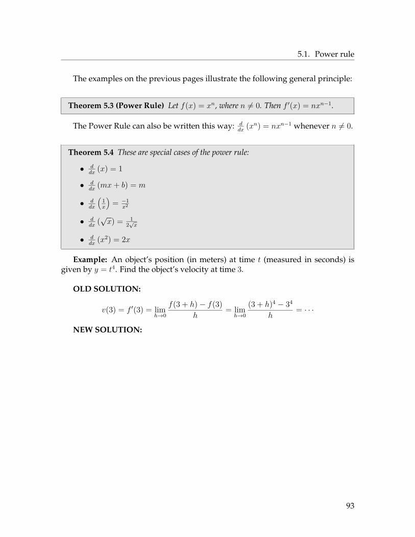
5.1. Power rule
The examples on the previous pages illustrate the following general principle:
Theorem 5.3 (Power Rule) Let f(x) = xn, where n 6= 0. Then f ′(x) = nxn−1.
The Power Rule can also be written this way: ddx
(xn) = nxn−1 whenever n 6= 0.
Theorem 5.4 These are special cases of the power rule:
• ddx
(x) = 1
• ddx
(mx+ b) = m
• ddx
(1x
)= −1
x2
• ddx
(√x) = 1
2√x
• ddx
(x2) = 2x
Example: An object’s position (in meters) at time t (measured in seconds) isgiven by y = t4. Find the object’s velocity at time 3.
OLD SOLUTION:
v(3) = f ′(3) = limh→0
f(3 + h)− f(3)h
= limh→0
(3 + h)4 − 34
h= · · ·
NEW SOLUTION:
93

5.2. Linearity rules
5.2 Linearity rulesQuestion: Do derivatives add/subtract/multiply/divide as expected?
In particular,
• Does (f + g)′ = f ′ + g′ ?
• Does (f − g)′ = f ′ − g′ ?
• Does (cf)′ = c · f ′ for a constant c?
• Does (fg)′ = f ′ · g′?
• Does(fg
)′= f ′
g′?
Theorem 5.5 (Sum Rule) If f and g are differentiable at x, then f+g is differentiableat x and (f + g)′(x) = f ′(x) + g′(x).
Proof of the Sum Rule: By definition, (f + g)(x) means f(x) + g(x). Now usingthe definition of the derivative,
(f + g)′(x) = limh→0
(f + g)(x+ h)− (f + g)(x)h
= limh→0
[f(x+ h) + g(x+ h)]− [f(x) + g(x)]h
= limh→0
f(x+ h)− f(x) + g(x+ h)− g(x)h
= limh→0
f(x+ h)− f(x)h
+ limh→0
g(x+ h)− g(x)h
= f ′(x) + g′(x).
Theorem 5.6 (Difference Rule) If f and g are differentiable at x, then f − g isdifferentiable at x and (f − g)′(x) = f ′(x)− g′(x).
Proof of the Difference Rule: similar to the proof of the Sum Rule.
94
5.2. Linearity rules
Theorem 5.7 (Constant Multiple Rule) If f is differentiable at x, then cf is differ-entiable at x for any constant c and (cf)′(x) = c · f ′(x).
Proof of the Constant Multiple Rule:
(cf)′(x) = limh→0
(cf)(x+ h)− (cf)(x)h
= limh→0
c f(x+ h)− c f(x)h
= limh→0
c[f(x+ h)− f(x)]h
= c limh→0
[f(x+ h)− f(x)]h
= c f ′(x).
Together, the Sum Rule, Difference Rule and Constant Multiple Rule are calledthe linearity rules for differentiation (for reasons that you learn in linear algebra(Math 322)).
Example: Compute the derivative of y = 3x2 + 2√x− 1.
Example: Let f(x) = 10x15 − 8x+ 7. Find f ′(−1).
95
5.2. Linearity rules
Example: Let y = 3 3√x− 2
3x3 + (3x− 2)2. Find dydx
.
WARNING: Products do not behave nicely under differentiation. Here is anexample to show why (fg)′ 6= f ′ · g′:
Suppose f(x) = x2 and g(x) = x3.
Then f ′(x) = 2x and g′(x) = 3x2.Therefore the product of the derivatives is f ′(x)g′(x) = (2x)(3x2) = 6x3.
BUT (fg)(x) = f(x)g(x) = x2x3 = x5.
Therefore the derivative of the product is (fg)′(x) =
96

5.3. Derivatives of sine, cosine and tangent
5.3 Derivatives of sine, cosine and tangentQuestion:
d
dx(sin x) = ?
d
dx(cosx) = ?
d
dx(tan x) = ?
To address these questions, we will use the limit definition of derivative foreach function. In computing these derivatives, we will need some trigonometricidentities, which are listed here for convenience:
sin(x+ h) = sin x cosh+ cosx sin h (5.1)
cosx = 1− 2 sin2(x
2
)(5.2)
cos(x+ h) = cos x cosh− sin x sin h (5.3)
tan(x+ h) = tan x+ tan h1− tan x tan h (5.4)
1 + tan2 x = sec2 x (5.5)
Example: Find the derivative of f(x) = sin x.
Solution:
d
dx(sin x) = lim
h→0
sin(x+ h)− sin xh
= limh→0
sin x cosh+ cosx sin h− sin xh
(by trig identity (5.1) above)
= limh→0
(cosx)sin hh
+ limh→0
(sin x)cosh− 1h
= cosx(
limh→0
sin hh
)+ sin x
(limh→0
cosh− 1h
).
97

5.3. Derivatives of sine, cosine and tangent
Side question 1:
limh→0
sin hh
= ?
Solution to side question 1:
1
1
This picture generates some shapes which sit inside one another. In particular, wehave
area of red triangle ≤ area of blue pizza wedge ≤ area of green triangle
12(base)(height) ≤ angle
2π (π radius2) ≤ 12(base)(height)
12(cosh)(sin h) ≤ h
2π (π12) ≤ 12(1)(tan h)
12 cosh sin h ≤ h
2 ≤ 12
sinhcosh
cosh sin h ≤ h ≤ sinhcosh
cosh ≤ hsinh ≤ 1
cosh
98
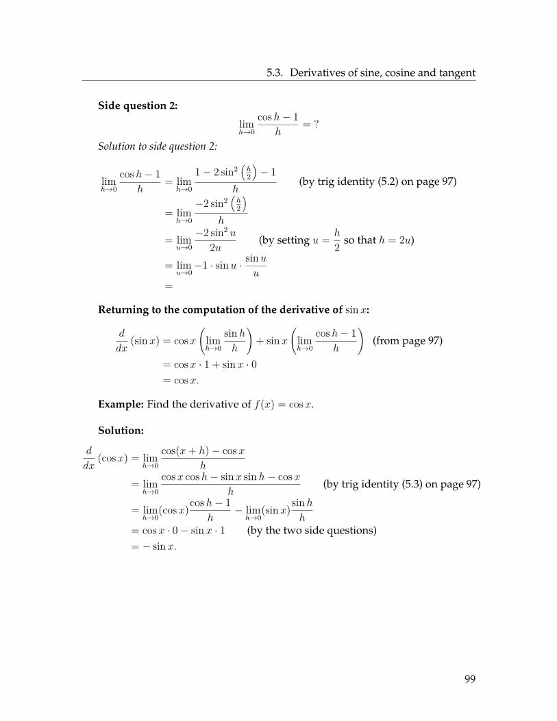
5.3. Derivatives of sine, cosine and tangent
Side question 2:
limh→0
cosh− 1h
= ?
Solution to side question 2:
limh→0
cosh− 1h
= limh→0
1− 2 sin2(h2
)− 1
h(by trig identity (5.2) on page 97)
= limh→0
−2 sin2(h2
)h
= limu→0
−2 sin2 u
2u (by setting u = h
2 so that h = 2u)
= limu→0−1 · sin u · sin u
u=
Returning to the computation of the derivative of sin x:
d
dx(sin x) = cos x
(limh→0
sin hh
)+ sin x
(limh→0
cosh− 1h
)(from page 97)
= cosx · 1 + sin x · 0= cosx.
Example: Find the derivative of f(x) = cos x.
Solution:
d
dx(cosx) = lim
h→0
cos(x+ h)− cosxh
= limh→0
cosx cosh− sin x sin h− cosxh
(by trig identity (5.3) on page 97)
= limh→0
(cosx)cosh− 1h
− limh→0
(sin x)sin hh
= cosx · 0− sin x · 1 (by the two side questions)= − sin x.
99

5.3. Derivatives of sine, cosine and tangent
Example: Find the derivative of f(x) = tan x.
Solution:
d
dx(tan x) = lim
h→0
tan(x+ h)− tan xh
= limh→0
tanx+tanh1−tanx tanh − tan x
h(by trig identity (5.4) on page 97)
= limh→0
tan x+ tan h− tan x(1− tan x tan h)h(1− tan x tan h)
= limh→0
tan x+ tan h− tan x+ tan2 x tan hh(1− tan x tan h)
= limh→0
tan h+ tan h tan2 x
h(1− tan x tan h)
= limh→0
tan h(1 + tan2 x)h(1− tan x tan h)
= limh→0
tan h sec2 x
h(1− tan x tan h) (by trig identity (5.5) on page 97)
= sec2 x · limh→0
sin hcosh · h · (1− tan x tan h)
= sec2 x · limh→0
( 1cosh
)(sin hh
)1
1− tan x tan h
= sec2 x · 11 · (1) · 1
1− tan x · 0 (by the first side question)
= sec2 x.
Theorem 5.8 (Derivatives of Sine, Cosine and Tangent)
d
dx(sin x) = cos x d
dx(cosx) = − sin x d
dx(tan x) = sec2 x
The derivatives of cotx, secx and cscx, as well as the derivatives of arctan xand arcsin x will be derived in the next chapter.
100

5.3. Derivatives of sine, cosine and tangent
Example: Find f ′(x) if f(x) = 2 sin x− 3 cosx+ 4.
Example: Find dydx
if y =√x3 + 5x− 2 tan x.
Example: Let y = 4 cos x− 2. Find dydx
∣∣∣x=π/2
.
101
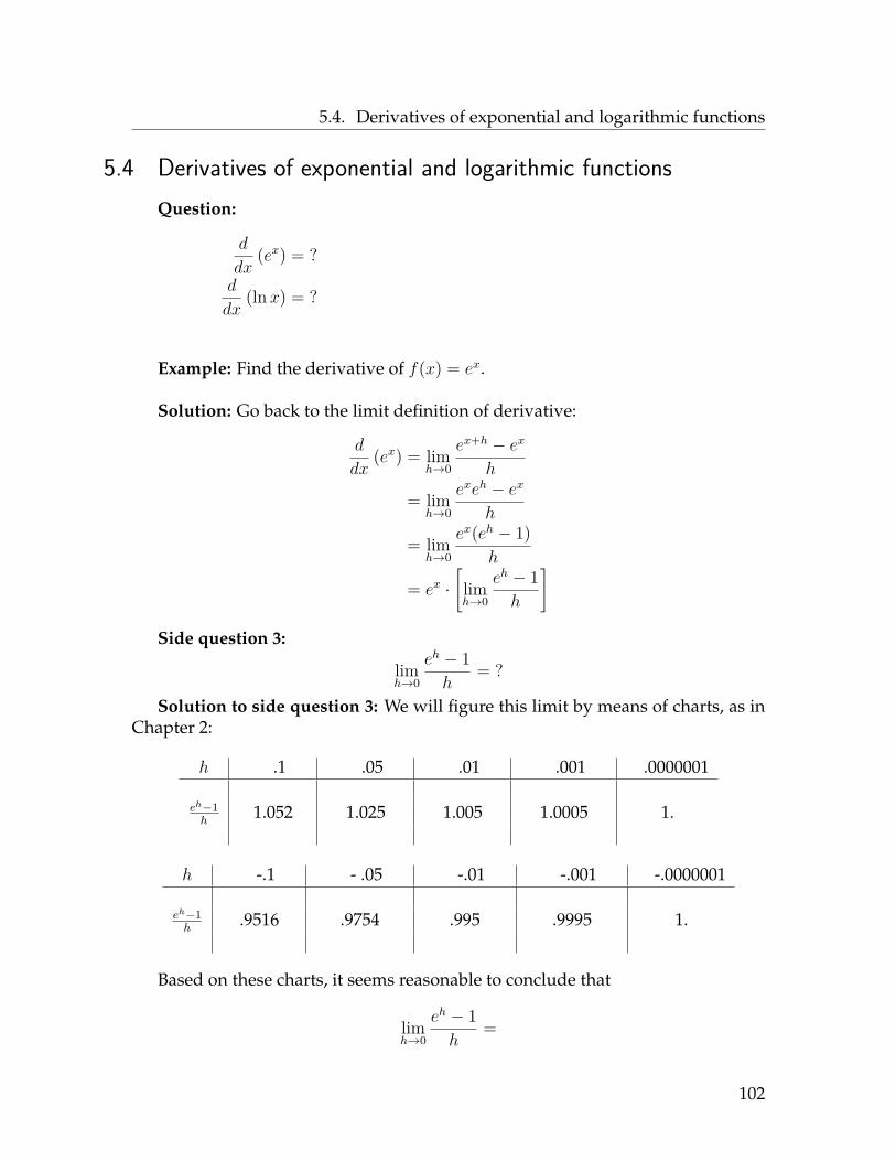
5.4. Derivatives of exponential and logarithmic functions
5.4 Derivatives of exponential and logarithmic functionsQuestion:
d
dx(ex) = ?
d
dx(ln x) = ?
Example: Find the derivative of f(x) = ex.
Solution: Go back to the limit definition of derivative:
d
dx(ex) = lim
h→0
ex+h − ex
h
= limh→0
exeh − ex
h
= limh→0
ex(eh − 1)h
= ex ·[limh→0
eh − 1h
]
Side question 3:
limh→0
eh − 1h
= ?
Solution to side question 3: We will figure this limit by means of charts, as inChapter 2:
h .1 .05 .01 .001 .0000001
eh−1h
1.052 1.025 1.005 1.0005 1.
h -.1 - .05 -.01 -.001 -.0000001
eh−1h
.9516 .9754 .995 .9995 1.
Based on these charts, it seems reasonable to conclude that
limh→0
eh − 1h
=
102

5.4. Derivatives of exponential and logarithmic functions
and therefore, returning to the example,
d
dx(ex) = ex
[limh→0
eh − 1h
]= ex · 1 = ex.
Theorem 5.9 (Derivative of the natural exponential function)) ddx
(ex) = ex.
In Section 6.5, we will derive the following rule for the natural logarithm func-tion:
Theorem 5.10 (Derivative of the natural logarithm function) ddx
(ln x) = 1x.
Example: Find the slope of the line tangent to the function f(x) = 3 ln x +√x
at x = 4.
Example: Find the derivative of y = 2ex − 4 sin x+ cosx− 2x6 − 1.
Example: Find the derivative of f(x) = log10 x.
103
5.5. Higher-order derivatives
5.5 Higher-order derivativesWe will see that many problems can be studied not just by differentiating a
function once, but by repeatedly differentiating it many times. First, we establishnotation to describe this procedure:
Definition 5.11 Let f : R→ R be a function.
• The zeroth derivative of f , sometimes denoted f (0), is just the function f itself.
• The first derivative of f , sometimes denoted f (1) or dydx
, is just f ′.
• The second derivative of f , denoted f ′′ or f (2) or d2ydx2 , is the derivative of f ′; in
other words, f ′′ = (f ′)′. The third derivative of f , denoted f ′′′ or f (3) or d3ydx3 ,
is the derivative of f ′′; in other words, f ′′′ = ((f ′)′)′.
• More generally, the nth derivative of f , denoted f (n) or dnydxn
,is the derivative off (n−1); in other words f (n) = ((((f ′)′) · · ·′)′.
Example: Let f(x) = 2x6. Find f ′′′(x).
Example: If y = cosx+ sin x, find d2ydx2
∣∣∣x=π/4
.
104

5.5. Higher-order derivatives
Physical interpretation of the second derivative
Suppose an object’s position on a number line after t units of time is given by f(t).Then
f ′(t) = rate of change of position = velocity
f ′′(t) = (f ′)′(t) = rate of change of velocity =
Example: A bee is flying back and forth along a number line, so that its positionafter t units of time is f(t) = −1
3 t3 + 3t2. What is the velocity of the object at the
instant where its acceleration is zero?
105
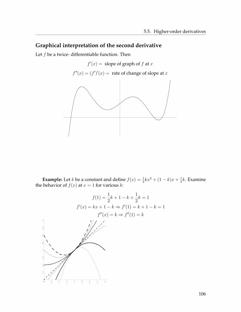
5.5. Higher-order derivatives
Graphical interpretation of the second derivative
Let f be a twice- differentiable function. Then
f ′(x) = slope of graph of f at x
f ′′(x) = (f ′)′(x) = rate of change of slope at x
Example: Let k be a constant and define f(x) = 12kx
2 + (1− k)x+ 12k. Examine
the behavior of f(x) at x = 1 for various k:
f(1) = 12k + 1− k + 1
2k = 1
f ′(x) = kx+ 1− k ⇒ f ′(1) = k + 1− k = 1f ′′(x) = k ⇒ f ′′(1) = k
0 1
4
1
2
3
41 5
4
3
2
7
42
1
4
1
2
3
4
1
5
4
3
2
7
4
2
106

5.5. Higher-order derivatives
Compiling information from the first and second derivative, we can determinethe general shape of a graph near a value x as follows:
f ′(x) > 0 f ′(x) < 0 f ′(x) = 0
f ′′(x) > 0
f ′′(x) < 0
f ′′(x) = 0
Before the days of Mathematica and graphics calculators, this is how peoplelearned to sketch the graphs of functions.
Example: Suppose f is some unknown function such that f(3) = −2, f ′(3) = 1and f ′′(3) = 2. Sketch a picture of what the graph of f looks like near x = 3:
-1 1 2 3 4 5
-3
-2
-1
1
2
3
107

5.5. Higher-order derivatives
Example: Suppose f is some function whose graph is given below:
-10 -9 -8 -7 -6 -5 -4 -3 -2 -1 1 2 3 4 5 6 7 8 9 10
-5
-4
-3
-2
-1
1
2
3
4
5
6
7
8
9
10
1. Estimate f(−6).
2. Estimate f ′(−6).
3. Estimate f ′′(−6).
4. Estimate f ′′(1).
5. Estimate f ′′(−3).
6. Estimate a value of x for which f ′(x) = 0 but f ′′(x) < 0.
7. Estimate a value of x for which f ′(x) < 0 but f ′′(x) > 0.
8. Is f ′′(9) positive, negative, or zero? Explain.
108

5.6. Homework exercises
5.6 Homework exercisesIn these problems (and all future problems), you may use rules to compute any
necessary derivatives (i.e. you do not have to use the limit definition).
1. Find dydx
if y = 3.
2. Find f ′(x) if f(x) = x6 + 2√x.
3. Find ddx
(3x− 4
5x + 1).
4. Find f ′(2) if f(x) = 2x3 + 2− x−1.
5. Find the derivative of h(x) = (x− 2)(x2 + 4).
6. Find the slope of the line tangent to y = 2x5/2 − x3/2 when x = 4.
7. Find the equation of the line tangent to f(x) = 3− x4 + 1x
when x = 1.
8. Suppose an object is traveling along a number line so that its position at timet is f(t) = 2t− 4t−2. Find the object’s velocity when t = 2.
9. Suppose an object’s position at time t is given by f(t) = 4t2 − 5t+ 2. Find alltimes t where the velocity of the object is −1.
10. Find f ′(x) if f(x) = 3 + 4x− 3√x.
11. Find ddx
√2x.
12. Find the derivative of f(x) = x2−1√x
.
13. Find f ′(x) if f(x) = 23 sin x+ 3
4 cosx− x2.
14. Find the derivative of y = 2− x− 4 tan x.
15. Let f(x) = cos x− 3. Find dfdx
∣∣∣x=π/4
.
16. Find the slope of the line tangent to y = 3 tan x− cosx when x = π6 .
17. Find the instantaneous velocity of an object at time t, if the object’s positionat time t is f(t) = 3t+ sin t.
18. Let g(x) = 4ex − 5x+ sin x. Find g′(x).
19. Find the derivative of f(x) = 4− 3x
+ 2 ln x.
20. Find the derivative of y = 3ex when x = 0.
21. Find the derivative of f(x) = ln x+ 4 3√x.
109
5.6. Homework exercises
22. Find the second derivative of f(x) = x3 − 1x
+ 4 sin x.
23. Find f ′′(x) if f(x) = 23x
6 − 2x
+ 4.
24. Let y = 2 sin t. Find d2ydt2
.
25. Find d2fdx2
∣∣∣x=1
if f(x) =(
2x
+√x).
26. If f(x) = 4ex − 5x4 + 3x, find f ′′(x).
27. Find the third derivative of f(x) = ln x when x = 2.
28. Find the 33rd derivative of f(x) = ex.
29. Let f(x) = sin x. Find f (801)(x).
30. Find the acceleration of an object at time 3, if the object’s position at time t isf(t) = 2t3 − t2 + 4t.
31. Find the acceleration of an object at time 2π3 , if the object’s velocity at time t is
v(t) = 3 sin t+ 2.
32. An object moves in such a fashion that its position after t units of time isf(t) = et − 2t. As time passes, is the object speeding up or slowing down?
33. An object moves in such a fashion that its position at time t is f(t) = t3 − 9t2.Find all times t where the acceleration of the object is zero.
34. Suppose f is some unknown function such that f(4) = 0, f ′(4) = −1 andf ′′(4) = 5. Sketch a picture of what the graph of f looks like near x = 4.
35. Suppose f is some unknown function such that f(−1) = 3, f ′(−1) = 0 andf ′′(−1) = −2
5 . Sketch a picture of what the graph of f looks like near x = −1.
36. Suppose f is some unknown function such that f(4) = 1, f ′(4) = 17 and
f ′′(4) = −23 . Sketch a picture of what the graph of f looks like near x = 4.
110

5.6. Homework exercises
37. Pictured below is the graph of some unknown function f . Use this graph toanswer the questions below:
-9 -8 -7 -6 -5 -4 -3 -2 -1 1 2 3 4 5 6 7 8 9
-5
-4
-3
-2
-1
1
2
3
4
5
6
7
8
Use the graph to determine, with justification, whether each of the followingquantities are positive, negative, or zero:
a) f(5)b) f ′(5)c) f ′′(5)
d) f(−6)e) f ′(−6)f) f ′′(−6)
g) f(−1)h) f ′(−1)i) f ′′(−1)
j) f(3)k) f ′(3)l) f ′′(3)
38. Pictured below is the graph of some unknown function g. Use this graph toanswer the questions below:
-9 -8 -7 -6 -5 -4 -3 -2 -1 1 2 3 4 5 6 7 8 9
-8
-7
-6
-5
-4
-3
-2
-1
1
2
3
4
5
6
7
8
Use the graph to answer the following questions:
a) Estimate g′′(1).b) Estimate g′′(5).c) Estimate g′′(−7).d) Find a value of x such that
g′(x) = 0 but g′′(x) > 0.
e) Find a value of x such thatg′(x) = 0 but g′′(x) < 0.
f) Find a value of x for which g′′(x)DNE.
111
5.6. Homework exercises
Answers
1. 0
2. 6x5 + 1√x
3. 3 + 45x−2
4. 974
5. 3x2 − 4x+ 4
6. 37
7. y = 3− 5(x− 1)
8. 3
9. t = 12
10. 4− 13x−2/3
11.√
22√x
12. 32x
1/2 − x−1/2
13. 23 cosx− 3
4 sin x− 2x
14. −1− 4 sec2 x
15. −√
22
16. 92
17. 3 + cos t
18. 4ex − 5 + cos x
19. 3x−2 + 2x
20. 3
21. 1x
+ 43x−2/3
22. 6x− 2x−3 − 4 sin x
23. 20x4 − 4x−3
24. −2 sin t
25. 154
26. 4ex − 60x2
27. 14
28. ex.
29. f(x) = cos x
30. 34
31. −32
32. Speeding up (since acceleration ispositive)
33. t = 3
34. Passes through (4, 0), slope of tangent line is −1 and lies above the tangentline at 4:
2 4 6 8
-3
-2
-1
1
2
3
4
35. Passes through (−1, 3), curved downward such that the “peak” of the graphis at (−1, 3):
112

5.6. Homework exercises
-3 -2 -1 0 1 2
1
2
3
4
36. Passes through (4, 1), slope of tangent line is 17 , and graph lies below the
tangent line:
1 2 3 4 5 6
-1.0
-0.5
0.0
0.5
1.0
1.5
2.0
37. a) f(5) = 0 (graph at x−axis at x = 5)
b) f ′(5) > 0 (graph going up from left to right)
c) f ′′(5) > 0 (graph lies above tangent line)
d) f(−6) > 0 (graph above x−axis at x = −6)
e) f ′(−6) > 0 (graph going up from left to right)
f) f ′′(−6) < 0 (graph lies below tangent line)
g) f(−1) > 0 (graph above x−axis at x = −1)
h) f ′(−1) < 0 (graph going down from left to right)
i) f ′′(−1) = 0 (graph is straight at x = −1)
j) f(3) < 0 (graph below x−axis at x = 3)
k) f ′(3) = 0 (tangent line horizontal)
l) f ′′(3) > 0 (graph lies above tangent line)
38. a) 0b) ≈ 1
4 (a small positive number)
c) ≈ −5 (a negative number)
d) x ≈ −5.25, x ≈ 8.1e) x ≈ −6.8, x ≈ −2.8f) x = −2
113
Chapter 6
Intermediate DifferentiationRules
6.1 Product ruleQuestion: What is d
dx(fg) (a.k.a. (fg)′) in terms of f , g, f ′ and g′?
Answer:
(fg)′(x) = limh→0
(fg)(x+ h)− (fg)(x)h
= limh→0
f(x+ h) g(x+ h)− f(x) g(x)h
= limh→0
f(x+ h) g(x+ h)− f(x) g(x+ h) + f(x) g(x+ h)− f(x) g(x)h
= limh→0
[f(x+ h) g(x+ h)− f(x) g(x+ h)
h+ f(x) g(x+ h)− f(x) g(x)
h
]
= limh→0
[g(x+ h)f(x+ h)− f(x)
h
]+ lim
h→0
[f(x)g(x+ h)− g(x)
h
]= g(x) f ′(x) + f(x) g′(x).
This proves the following theorem:
Theorem 6.1 (Product Rule) Let f and g be differentiable at x. Then fg is differen-tiable at x and
(fg)′(x) = f ′(x) g(x) + g′(x) f(x).
114

6.1. Product rule
The Product Rule says, in English, the following:
the derivative of a product is “the derivative of the first times the second plus thederivative of the second times the first”.
Example: Find y′ if y = 3x2 sin x.
Example: Find f ′(0) if f(x) = (2x3 + 4x− 1) tan x.
Example: Find d2ydx2 if y = x4ex.
Solution: First, by the Product Rule,
dy
dx= 4x3ex + exx4.
Example: Find f ′(x) if f(x) = cos2 x.
115

6.2. Quotient rule
6.2 Quotient ruleTheorem 6.2 (Quotient Rule) Let f and g be differentiable at x, where g(x) 6= 0.Then f
gis differentiable at x and
(f
g
)′(x) = f ′(x) g(x)− g′(x) f(x)
[g(x)]2 .
The proof of this is similar to the proof of the Product Rule and is omitted.
The Quotient Rule says, in English, the following:
the derivative of a quotient is “the derivative of the top times the bottom minus thederivative of the bottom times the top, all over the bottom squared”.
Example: Find g′(x) if g(x) = 2√x−3x+15 lnx .
Example: Let f(x) = x2+1x2−1 . Find the slope of the line tangent to f when x = 0.
116

6.2. Quotient rule
Example: Find d2ydx2 if y = 3ex
x.
Example: Find f ′(x) if f(x) = 3 tanx+6x2−5x+2−4 cosx−3x−2/3+2 .
117
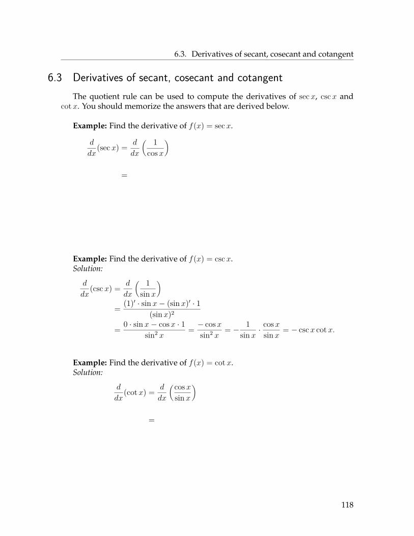
6.3. Derivatives of secant, cosecant and cotangent
6.3 Derivatives of secant, cosecant and cotangentThe quotient rule can be used to compute the derivatives of secx, cscx and
cotx. You should memorize the answers that are derived below.
Example: Find the derivative of f(x) = secx.
d
dx(secx) = d
dx
( 1cosx
)
=
Example: Find the derivative of f(x) = cscx.Solution:
d
dx(cscx) = d
dx
( 1sin x
)= (1)′ · sin x− (sin x)′ · 1
(sin x)2
= 0 · sin x− cosx · 1sin2 x
= − cosxsin2 x
= − 1sin x ·
cosxsin x = − cscx cotx.
Example: Find the derivative of f(x) = cot x.Solution:
d
dx(cotx) = d
dx
(cosxsin x
)
=
118

6.3. Derivatives of secant, cosecant and cotangent
Theorem 6.3 (Derivatives of secant, cosecant and cotangent)
d
dx(secx) = sec x tan x d
dx(cscx) = − cscx cotx d
dx(cotx) = − csc2 x
Example: Find the instantaneous rate of change of the function f(x) = 2x secx+1 when x = 0.
Example: Let y = secx+3 cotxx−sinx . Find dy
dx.
119

6.3. Derivatives of secant, cosecant and cotangent
Example: Suppose an object’s position, measured in feet, at time t, measuredin seconds, is given by f(t) = et cos t. Find the object’s velocity and acceleration attime 0.
Example: Find ddt
(2√t csc t
).
Example: Find g′(π3
)if g(t) = t2 sin t.
Solution: First, by the Product Rule, g′(t) = 2t sin t+ (cos t)t2.
⇒ g′(π
3
)= 2
(π
3
)sin
(π
3
)+ cos
(π
3
)·(π
3
)2
= 2(π
3
) √32 + 1
2
(π2
9
)
= π√
33 + π2
18 .
120

6.4. Chain rule
6.4 Chain ruleQuestion: Given differentiable functions f and g, find the derivative of f ◦ g in
terms of f , f ′, g and g′.
Motivating example:
Suppose Mrs. Young is moving 5 times as fast as Mrs. Underwood.
Suppose also that Mrs. Underwood is moving 3 times as fast as Mrs. Xavier.
What is the relationship between Mrs. Young’s speed and Mrs. Xavier’s speed?
Answer:
In the language of derivatives, the motivating example becomes the followingquestion:
“Ifdy
du= 5 and
du
dx= 3, what is
dy
dx?”
The answer is found as follows:
The general idea described here is what is called the Chain Rule:
Theorem 6.4 (Chain Rule, Leibniz notation)
dy
dx= dy
du· dudx.
121
6.4. Chain rule
Example: Find dydx
if y =√
sin x.
Continuing with this example, let F (x) =√
sin x. Then,
122

6.4. Chain rule
Theorem 6.5 (Chain Rule, prime notation) If f and g are differentiable functions,then f ◦ g is differentiable and
(f ◦ g)′(x) = f ′(g(x)) g′(x).
I like to think of a composition as having an “outside” part (the f ) and an “in-side” part (the g). The Chain Rule says, in English, the following:
the derivative of a composition is “the derivative of a composition is the derivative ofthe outside, with the inside plugged in, times the derivative of the inside”.
Example: Find ddx
[(1x− sin x
)4].
Example: Find y′ if y =√
3x+ 4.
123

6.4. Chain rule
Example: Find the equation of the line tangent to f(x) = (3x2 − 3x− 1)9 whenx = 1.
Example: If an object’s position at time x is given by f(x) = e−x, find the object’svelocity and acceleration at time x.
Example: Let y = cos(x2). Find d2ydx2 .
124

6.4. Chain rule
When to use the Product Rule, as opposed to the Chain Rule
Example:d
dx
(x2 sin x
)vs.
d
dx
(sin x2
)
Use of the Chain Rule in conjunction with other rules
Example: Find the derivative of each of these functions:
1. y = 2x ln(4x2 + 1)
2. f(x) = x2 cos3 x− 4x tan2 x
125
6.4. Chain rule
3. y = (ex+x2−2)3
(x−3−1)3/2
4. f(x) = sin(
lnx−2cosx+x
)Solution: Start with the Chain Rule, because “sin” doesn’t mean anything byitself:
f ′(x) = outside′(inside) · (inside)′
= cos(
ln x− 2cosx+ x
)·(
ln x− 2cosx+ x
)′
Now use the Quotient Rule to compute the inside′:
f ′(x) = cos(
ln x− 2cosx+ x
)·
1x(cosx+ x)− (− sin x+ 1)(ln x− 2)
(cosx+ x)2
5. f(x) = cos(√
secx)
126

6.4. Chain rule
Logarithmic differentiation
Example: Suppose f(x) = xx. What is f ′(x)?
Incorrect solution: Try the Power Rule: f ′(x) = x xx−1 = xx.
Reason this is incorrect:
Correct solution:
In general, to differentiate a function of the form f(x)g(x), first rewrite the func-tion using the change of base formula for exponentials:
f(x)g(x) = eg(x) ln f(x)
Then differentiate using the Chain and Product Rules. This procedure is calledlogarithmic differentiation.
Example: Find the derivative of f(x) = (x2 − 2)cosx.
127

6.5. Implicit differentiation
6.5 Implicit differentiationAnother application of the Chain Rule
Suppose z = sin y and y = f(x), where you don’t know what the function f is.
dz
dx= ?
Answer: By the Chain Rule,
Example: Suppose that y is some unknown function of x. Find ddx
(y2 + 6y − 2).
Note: If y is a constant, rather than a function of x, then ddx
(y2 + 6y − 2) =
Example: ddx
(x4 − sin y + 5) = ?
128

6.5. Implicit differentiation
Example: ddx
(y3 sin x) = ?
Implicit differentiation of equations
Example: Consider the equation x2 + y2 = 25.This equation is not a function, for two reasons:
1.
2.
Suppose you wanted to write the equation of the tangent line to x2 + y2 = 25 atsome point. You would need to compute dy
dxat that point to get the slope. But
which equation do you differentiate:
y =√
25− x2 or y = −√
25− x2
In this example, the choice is obvious:
129

6.5. Implicit differentiation
But in general, there is no way to tell which equation to use. Consider theequation
4(y2 − x2) = y4.
If you solve for y, you will get four different solutions:
There’s no (easy) way to tell which solution goes with which graph.
Question: Is there a way to compute dydx
for some equation without solving fory in terms of x?
Answer: Yes. The method is called implicit differentiation. To implement it,start with the equation and differentiate both sides with respect to x (i.e. “take d
dx
of both sides”).
General procedure to implement implicit differentiation:
1. Take ddx
of both sides (as with the examples earlier).
2. If you are given x and/or y values, plug them in.
3. Solve for dydx
.
130

6.5. Implicit differentiation
Example: Find the slope of the line tangent to the circle x2 +y2 = 25 at the point(3,−4).
Follow up question: In the preceding example, how would you determinethe value of the second derivative at (3,−4) (i.e. how would you measure theconcavity of the circle)?
131

6.5. Implicit differentiation
Example: Find dydx
∣∣∣x=3,y=3
for the equation x3 + y3 − 6xy = 0.
Example: Find dydx
for the equation x+ e2xy = 10.
132
6.5. Implicit differentiation
Implicit differentiation can be used to justify the fact that the derivative of ln xis 1
xas follows:
y = ln x⇔ ey = x
d
dx(ey) = d
dx(x)
Example: Find the derivative of f(x) = arctan x.
Solution: As in the previous example, rewrite the function and use implicitdifferentiation:
y = arctan x⇔ x = tan y
1 = sec2 ydy
dx
1 = (1 + tan2 y) dydx
1 = (1 + x2) dydx
11 + x2 = dy
dx
Example: Find the derivative of f(x) = arcsin x.
133

6.5. Implicit differentiation
The method of the last three examples generalizes to the following theorem:
Theorem 6.6 (Inverse Function Theorem) If y = f(x) is a differentiable and in-vertible function such that f ′(x) 6= 0, then
(f−1)′(y) = 1f ′(x) .
Associated picture:
0 2 4 6 8 10
2
4
6
8
10
Example: Suppose f is some unknown invertible function such that f(6) = 2and f ′(6) = 3. Find (f−1)′(2).
How this theorem relates to the preceding three examples:
Function f Inverse f−1 Derivative of f Derivative off−1
y = f(x) = ex f−1(y) = ln y f ′(x) = ex = y (f−1)′(y) = 1y
y = f(x) = tan x f−1(y) = arctan y f ′(x) = sec2 x = 1 + y2 (f−1)′(y) = 11+y2
y = f(x) = sin x f−1(y) = arcsin y f ′(x) = cos x =√
1− y2 (f−1)′(y) = 1√1−y2
134

6.6. Summary of differentiation rules
6.6 Summary of differentiation rulesDerivatives of functions that you should memorize:
Constant Functions ddx
(c) = 0
Power Rule ddx
(xn) = nxn−1 (so long as n 6= 0)
Special cases of the Power Rule: ddx
(mx+ b) = m
ddx
(√x) = 1
2√x
ddx
(1x
)= −1
x2
ddx
(x2) = 2x
Trigonometric Functions ddx
(sin x) = cos xddx
(cosx) = − sin xddx
(tan x) = sec2 x
ddx
(cotx) = − csc2 x
ddx
(secx) = sec x tan xddx
(cscx) = − cscx cotx
Exponential Function ddx
(ex) = ex
Natural Log Function ddx
(ln x) = 1x
Inverse Trig Functions ddx
(arctan x) = 1x2+1
ddx
(arcsin x) = 1√1−x2
Rules that tell you how to differentiate more complicated functions:
Sum Rule (f + g)′(x) = f ′(x) + g′(x)
Difference Rule (f − g)′(x) = f ′(x)− g′(x)
Constant Multiple Rule (kf)′(x) = k · f ′(x) for any constant k
Product Rule (fg)′(x) = f ′(x) g(x) + g′(x) f(x)
Quotient Rule(fg
)′(x) = f ′(x) g(x)−g′(x) f(x)
[g(x)]2
Chain Rule (f ◦ g)′ (x) = f ′(g(x)) g(x)
Inverse Function Theorem If y = f(x) and f is invertible,
then (f−1)′(y) = 1f ′(x)
135

6.7. Homework exercises
6.7 Homework exercises1. Let g(x) = (x2 + 1)(x2 − 3x+ 4). Find g′(x).
2. Let f(x) = 4x2 ln x. Find dfdx
.
3. Find the derivative of f(x) = xx2−x+1 .
4. Find g′(1) if g(x) = x√x+1 .
5. Differentiate f(x) = sinxx2 .
6. Find the derivative of f(x) =√x sin x.
7. Find dydx
if y = (2x3 − x−2/3)ex.
8. Find the instantaneous velocity of an object at time t = π3 , if the position of
the object is given by f(t) = t2 sin t.
9. Find ddx
[(1
4x2 − 1) ln x
].
10. Find the second derivative of f(x) = x ln x.
11. Find f ′(2) if f(x) = 2 sin x 5√x.
12. Differentiate f(x) = x2+1x3−1 .
13. Find y′ if y = cosx√x
.
14. Find the slope of the line tangent to the graph of f(x) = 4 cosx sin x whenx = π
4 .
15. Find the acceleration of a particle at time t, given that the particle’s positionat time t is 3t2−4
t2+1 .
16. Let y = 8x9−sinxlnx+5 . Find dy
dx.
17. Find f ′(π) if f(x) = x2 sin x.
18. Find the equation of the line tangent to the graph of y = cosxx
when x = π/2.
19. Find the equation of the line tangent to f(x) = (x − 1)(x2 − 2) at the point(0, 2).
20. Suppose f ′′′(x) = 2x cosx. Find f (4)(x).
21. Suppose f and g are functions such that f(3) = 2, f ′(3) = −1, g(3) = 4 andg′(3) = 2. Find (fg)′(3) and
(fg
)′(3).
136

6.7. Homework exercises
In Problems 22-29, find the derivative of the given function.
22. f(x) = 2 cotx
23. y = 3x4 cscx
24. f(x) = −1x2 + secx− 4 sin x
25. f(x) = secxx
26. y = x sin x− 2xcotx
27. f(x) = 14√x+ 3− 5 cscx
28. y = 4√x+ 6 tan x− 3 cotx
29. f(x) = ln x sin x
30. a) Find the derivative of f(x) = (x− 3)−3 using the Chain Rule.
b) Find the derivative of f(x) = (x− 3)−3 by rewriting the function (to getrid of the negative exponent) and using the Quotient Rule.
c) Verify that the answers you got in (a) and (b) are the same.
31. Find the derivative of y = (2x− 3)8.
32. Find f ′(2) if f(x) =√
8− x.
33. Find dydx
if y = 3√
4x2 + 5.
34. Differentiate f(x) = csc2 x.
35. Find the derivative of f(x) = 4 ln(cosx).
36. Suppose an object’s position at time t is cos(
3πt2
). Find the velocity of the
object at the instant t = 1.
37. Find d2ydx2 if y = (5x− 1)−3.
38. Find the derivative of f(x) = e5x.
39. Find the derivative of f(x) = sin(x2 ).
40. Find the slope of the line tangent to f(x) = 3 cos(x2) when x = 0.
41. Find y′ if y = sec 1x− x2.
42. Let f(x) = 14 sin4(2x). Find f ′(x).
43. Find the equation of the line tangent to f(x) =√x2 + 2x+ 8 when x = 2.
44. Suppose an object’s position at time t is given by f(t) = (t2 + 3)e2t. Find thevelocity of the object when t = 0.
45. Suppose f and g are functions such that f(1) = 4, f ′(1) = −3, f(3) = 2,f ′(3) = 5, g(3) = 1 and g′(3) = 2. Find (fg)′(3) and (f ◦ g)′(3).
137
6.7. Homework exercises
46. Suppose dydu
= 3 and dudx
= 6. What is dydx
?
47. Suppose dydx
= 8 and dudx
= 4. What is dydu
?
48. Suppose dydv
= 5 and dxdv
= 3. What is dydx
?
In Problems 49-66, find the derivative of the given function.
49. f(x) = x2(x− 2)4
50. f(x) = x√
4− x2
51. f(x) =(
1−2xx+1
)5
52. f(x) =√x cosx
53. f(x) = x3−2√x6+1
54. f(x) = sin(x+1x−1
)55. f(x) = cos(tan x)
56. f(x) = cos x tan x
57. f(x) = cos(x tan x)
58. y = cot4(5x+ 1)
59. y =√
xx−1
60. f(x) = esinx
61. f(x) = e2x−5
62. g(x) = ln(x2 + 8x+ 5)
63. f(x) = sec2(4x)
64. f(x) = 3x−√x+ x2 sin x
65. f(x) = 2 + ln x− x7e4x
66. f(x) = 3+x2 cotx4√x−sin(ex)
67. f(x) = x2x
68. f(x) = 5x
69. f(x) = xsinx
70. f(x) = (tan x)2x
In problems 71-76, find the derivative dydx
.
71. x2 + y2 = 49
72. x3 − xy + y2 = 4
73. sin x+ 2 cos 2y = 1
74. x = cos(xy)
75. ex = xey
76. ln y = cosx
77. Find the slope of the line tangent to x2y − y3 = −8 at the point (0, 2).
78. Find the equation of the line tangent to (x2 + y2)2 = 4x2y at the point (1, 1).
79. Find the equation of the line tangent to the elllipse x2
2 + y2
8 = 1 at (1, 2).
138

6.7. Homework exercises
80. Find the slope of the line tangent to the hyperbola y2
6 −x2
8 = 1 at the point(−2,−3).
81. Find d2ydx2 if x2 + y2 = 4.
Hint: First find dydx
, then take the derivative of that expression implicitly.
82. Find d2ydx2 if y2 = sin x.
In Problems 83-88, find the derivative of the given function.
83. f(x) = arctan 2x
84. f(x) = x3 arctan x
85. f(x) = arcsin x− 1x
+ ln x− 2
86. f(x) = 4 arcsin 3x
87. f(x) = x arctan 2x
88. f(x) = earctanx
89. Suppose f is an invertible function such that f(3) = 7. If f ′(3) = 4, what is(f−1)′(2)?
90. Suppose f is some invertible function such that f(0) = 0 and f ′(x) = 2e−x2 .Find (f−1)′(0).
91. Suppose f is some invertible function such that f(1) = 12 and f ′(x) = e−x
2 .Find (f−1)′(1
2).
139

6.7. Homework exercises
Answers
1. 2x(x2 − 3x+ 4) + (2x− 3)(x2 + 1)
2. 8x ln x+ 4x
3. x2−x+1−x(2x−1)(x2−x+1)2 .
4. 38
5. x2 cosx−2x sinxx4
6. 12√x
sin x+√x cosx
7. (6x2 + 23x−5/3)ex + (2x3 − x−2/3)ex
8. π√
33 + π2
18
9. 12x ln x+ (1
4x2 − 1) 1
x
10. 1x
11. 2 5√
2 cos 2 + 252−4/5 sin 2
12. 2x(x3−1)−3x2(x2+1)(x3−1)2
13.−√x sinx− 1
2√x
cosxx
.
14. 0
15. 14(1−3x2)(1+x2)3
16. (72x8−cosx)(lnx+5)− 1x
(8x9−sinx)(lnx+5)2
17. −π2.
18. y = − 2π(x− π
2 )
19. y = 2− 2x
20. 2 cosx− 2x sin x
21. (fg)′(3) = 0;(fg
)′(3) = −1
2 .
22. −2 csc2 x
23. 12x3 cscx− 3x4 cscx cotx
24. 2x−3 + secx tan x− 4 cosx
25. x secx tanx−secxx2
26. sin x+ x cosx− 2 cotx+2x csc2 xcot2 x
27. 18√x
+ 5 cscx cotx
28. 14x−3/4 + 6 sec2 x+ 3 csc2 x
29. 1x
sin x+ ln x cosx
30. −3(x− 3)−4
31. 16(2x− 3)7
32. −12√
6
33. 8x3 (4x2 + 5)−2/3
34. −2 csc2 x cotx
35. −4 tan x
36. 3π2
37. 300(5x− 1)−5
38. 5e5x
39. 12 cos x
2
40. 0
41. −1x2 sec 1
xtan 1
x− 2x
42. 2 sin3(2x) cos(2x)
43. y = 4 + 34(x− 2)
44. 6
45. (fg)′(3) = 9; (f ◦ g)′(3) = −6.
46. 18
47. 2
48. 53
140

6.7. Homework exercises
49. 2x(x− 2)4 + 4(x− 2)3x2
50.√
4− x2 − x2√
4−x2
51. 5(
1−2xx+1
)4· −2(x+1)−(1−2x)
(x+1)2
52. 12√x cosx · (cosx− x sin x)
53.3x2√x6+1− 6x5
2√x6+1
(x3−2)
x6+1
54. cos(x+1x−1
)· −2
(x−1)2
55. − sin(tan x) sec2 x
56. − sin x tan x+ cosx sec2 x
57. − sin(x tan x) · (tan x+ x sec2 x)
58. −20 cot3(5x+ 1) csc2(5x+ 1)
59. 12√
xx−1· −1
(x−1)2
60. esinx cosx
61. 2e2x−5
62. 2x+8x2+8x+5
63. 8 sec2(4x) tan(4x)
64. −3x2 − 1
2√x
+ 2x sin x+ x2 cosx
65. 1x− 7x6e4x − 4x7e4x
66.(2x cotx−x2 csc2 x)(4
√x−sin(ex))−( 2√
x−ex cos(ex))(3+x2 cotx)
(4√x−sin(ex))2
67. x2x(2 ln x+ 2)
68. 5x ln 5
69. xsinx cosx ln x+ xsinx−1 sin x
70. 2(tan x)2x ln(tan x) + 2x(tan x)2x secx cscx
71. −xy
72. y−3x2
2y−x
73. cosx4 sin 2y
74. − cscxy−yx
75. ex+2y−ey−xey
76. −y sin x
77. 0
78. y = 1
79. y = 2− 2(x− 1)
80. 12
81. −4y3 .
82. −2y2 sinx−cos2 x4y3
83. 21+(2x)2
84. 3x2 arctan x+ x3
x2+1
85. 1√1−x2 + 1
x2 + 1x
86. 12√1−9x2
87. arctan 2x+ 2x1+4x2
88. earctanx · 11+x2
89. 14
90. 12
91. e
141

Chapter 7
Optimization Analysis
7.1 What is an optimization problem?There are many situations in the real world where you need to determine how
to make some quantity as large or as small as possible. Here are some examples:
Example 1: If an archer shoots an arrow into the air at angle θ from the ground,it will travel a horizontal distance of v sin 2θ
g, where v and g are constants. At what
angle should the archer shoot the arrow to make it travel as far as possible? (Equiv-alently, what is the maximum range of the archer?)
Example 2: An epidemic spreads through a population in such a way that thenumber of infected people, I , is a function of the number of susceptible people, x,by the formula
I(x) = 4 ln(x
30
)− x+ 30.
What is the maximum number of people who will become infected?
Example 3: A patient’s temperature change T , when given dose d of somemedicine, is given by
T =(
1− d
3
)d2
What dosage maximizes this temperature change?
Example 4: A farmer has 50 feet of fence with which to build a rectangular pen.What dimensions of the pen make its area as big as possible?
142
7.1. What is an optimization problem?
Example 5: A box with a square base and no top is to be constructed from ply-wood. If there is 48 square feet of plywood available, and if the length, width andheight of the box must be at least 1 foot, what is the largest volume of a box thatcan be made?
These examples have some important characteristics in common:
1. In each example, there is some quantity you are allowed to “choose”; thisquantity is the variable.
2. In each example, there is a second quantity which depends on the variable.This quantity is called the utility; the goal of the problem is to maximize orminimize the utility.
Any problem which asks you to maximize or minimize a utility function de-pending on one (or more) variables is called an “optimization problem”.
Here is the variable and utility for each of the first three examples on the previ-ous page:
Variable Utility
Example 1
Example 2
Example 3
Examples 4 and 5 are a little different, because there are two variables presentin the problem.
In Math 220, we can only solve an optimization problem with two or morevariables if there is some extra information which relates the variables. This extrainformation is called a constraint on the variables. (Take Math 320 - Calculus III -if you want to learn how to solve general optimization problems with more thanone variable.)
143
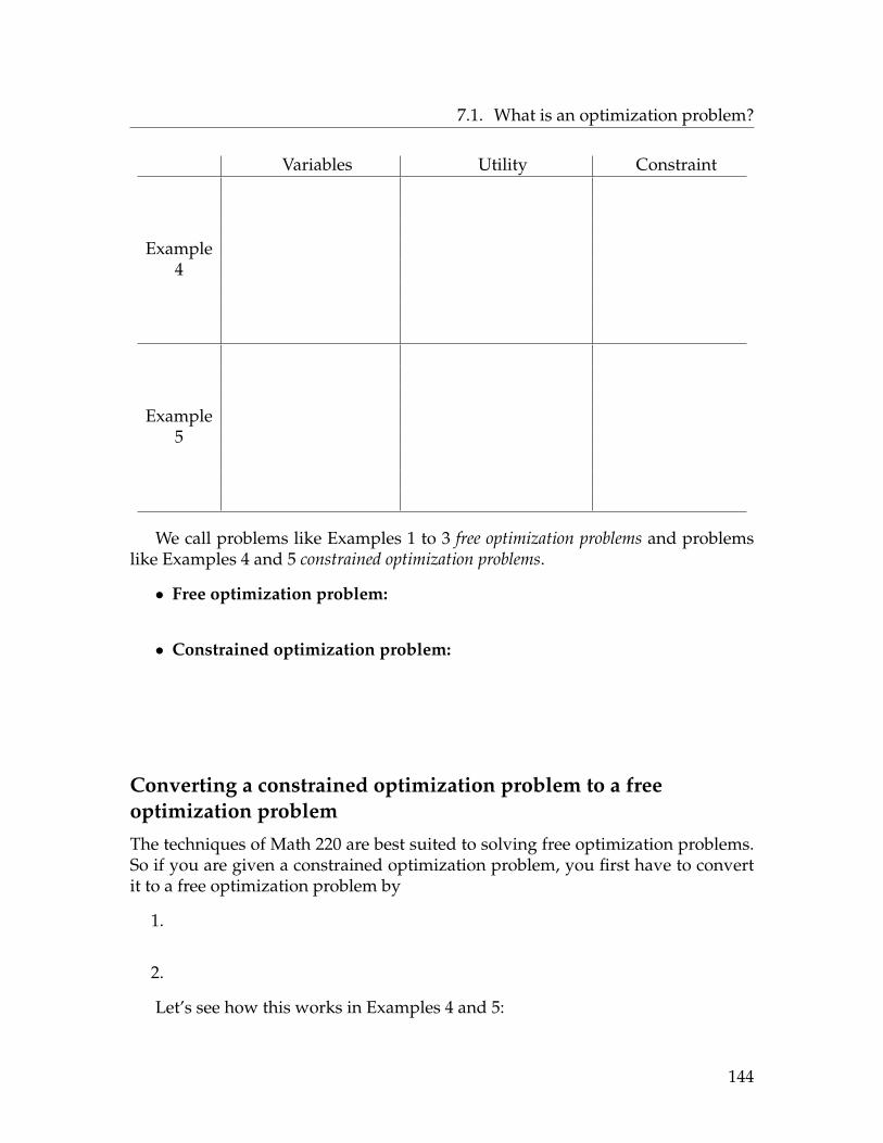
7.1. What is an optimization problem?
Variables Utility Constraint
Example4
Example5
We call problems like Examples 1 to 3 free optimization problems and problemslike Examples 4 and 5 constrained optimization problems.
• Free optimization problem:
• Constrained optimization problem:
Converting a constrained optimization problem to a freeoptimization problem
The techniques of Math 220 are best suited to solving free optimization problems.So if you are given a constrained optimization problem, you first have to convertit to a free optimization problem by
1.
2.
Let’s see how this works in Examples 4 and 5:
144

7.1. What is an optimization problem?
Example 4: (variables x and y) (utility A = xy) (constraint 2x+ 2y = 50)
Example 5: (variables x and y) (utility V = x2y) (constraint x2 + 4xy = 20)
Henceforth we will focus on solving free optimization problems. Keep in mindthat whenever you are given a constrained optimization problem, the first step isto convert it to a free optimization as above.
145
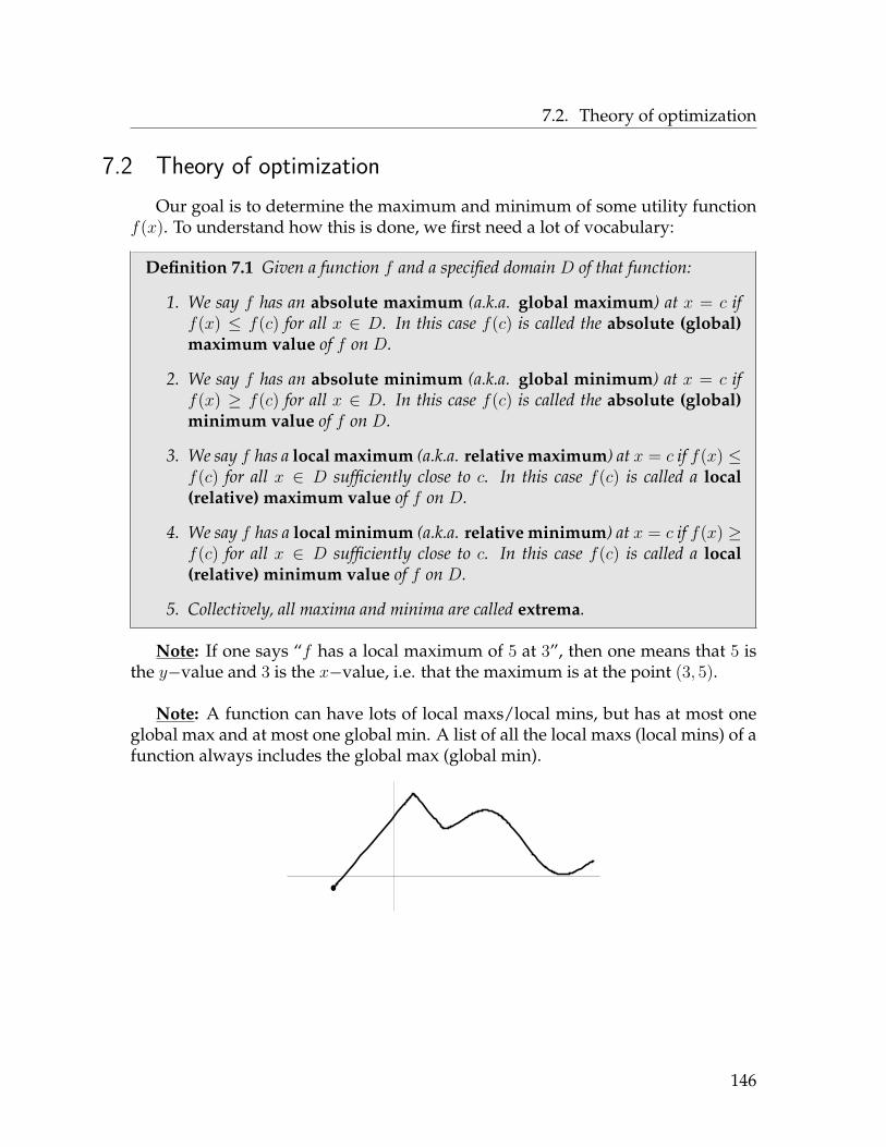
7.2. Theory of optimization
7.2 Theory of optimizationOur goal is to determine the maximum and minimum of some utility function
f(x). To understand how this is done, we first need a lot of vocabulary:
Definition 7.1 Given a function f and a specified domain D of that function:
1. We say f has an absolute maximum (a.k.a. global maximum) at x = c iff(x) ≤ f(c) for all x ∈ D. In this case f(c) is called the absolute (global)maximum value of f on D.
2. We say f has an absolute minimum (a.k.a. global minimum) at x = c iff(x) ≥ f(c) for all x ∈ D. In this case f(c) is called the absolute (global)minimum value of f on D.
3. We say f has a local maximum (a.k.a. relative maximum) at x = c if f(x) ≤f(c) for all x ∈ D sufficiently close to c. In this case f(c) is called a local(relative) maximum value of f on D.
4. We say f has a local minimum (a.k.a. relative minimum) at x = c if f(x) ≥f(c) for all x ∈ D sufficiently close to c. In this case f(c) is called a local(relative) minimum value of f on D.
5. Collectively, all maxima and minima are called extrema.
Note: If one says “f has a local maximum of 5 at 3”, then one means that 5 isthe y−value and 3 is the x−value, i.e. that the maximum is at the point (3, 5).
Note: A function can have lots of local maxs/local mins, but has at most oneglobal max and at most one global min. A list of all the local maxs (local mins) of afunction always includes the global max (global min).
146
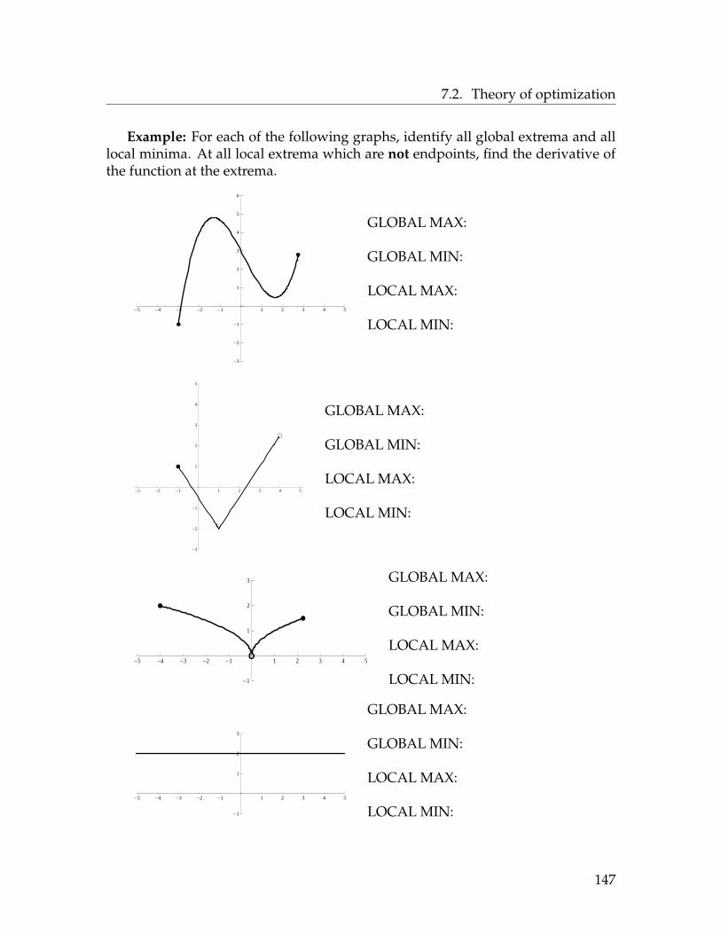
7.2. Theory of optimization
Example: For each of the following graphs, identify all global extrema and alllocal minima. At all local extrema which are not endpoints, find the derivative ofthe function at the extrema.
-5 -4 -3 -2 -1 1 2 3 4 5
-3
-2
-1
1
2
3
4
5
6
GLOBAL MAX:
GLOBAL MIN:
LOCAL MAX:
LOCAL MIN:
-3 -2 -1 1 2 3 4 5
-3
-2
-1
1
2
3
4
5
GLOBAL MAX:
GLOBAL MIN:
LOCAL MAX:
LOCAL MIN:
-5 -4 -3 -2 -1 1 2 3 4 5
-1
1
2
3 GLOBAL MAX:
GLOBAL MIN:
LOCAL MAX:
LOCAL MIN:
-5 -4 -3 -2 -1 1 2 3 4 5
-1
1
2
3
GLOBAL MAX:
GLOBAL MIN:
LOCAL MAX:
LOCAL MIN:
147

7.2. Theory of optimization
-8 -7 -6 -5 -4 -3 -2 -1 1 2 3 4 5 6 7 8
-8
-7
-6
-5
-4
-3
-2
-1
1
2
3
4
5
6
7
8
GLOBAL MAX: 6 at x = −4
GLOBAL MIN: DNE
LOCAL MAX:{
2.5 at x = 26 at x = −4
LOCAL MIN: −3 at x = −1
Definition 7.2 An optimization problem is a problem in which you are asked tofind the absolute maximum and/or absolute minimum value of a function on somedomain.
Question 1: Does a function necessarily have an absolute maximum and/orabsolute minimum? (In other words, does a generic optimization problem neces-sarily have a solution?)
Theorem 7.3 (Max-Min Existence Theorem) If f is continuous on a closed andbounded interval [a, b], then f has a global maximum value and a global minimumvalue on that interval.
Note: The preceding theorem may fail if f is not cts, or if the interval is notclosed, or if it is not bounded.
Question 2: How do you find the absolute maximum value and/or absoluteminimum value of some function on some domain? (In other words, how do yousolve an optimization problem?)
148

7.2. Theory of optimization
Definition 7.4 A critical point (a.k.a. CP) of a function f is a number c such thatf ′(c) = 0 or f ′(c) does not exist.
Note: Critical points are numbers, not points. (They are the x-coordinates ofpoints).
Theorem 7.5 (Critical Point Theorem) All local extrema of a function (and there-fore all global extrema) on an interval must occur at
1. endpoints of the interval, and/or
2. critical points of f lying in the interval.
Note: Not all critical points are local extrema.
The Critical Point Theorem suggests a method of finding the global extrema ofa function on an interval:
To optimize f on interval [a, b]:
1. Find the critical points of f by(a) setting f ′(x) = 0 and solving for x, and(b) finding all x for which f ′(x) DNE.
2. Plug each of the critical points which are in [a, b], as well as the twoendpoints a and b, into the function f .
The largest number you get is the absolute maximum, and the smallestnumber you get is the absolute minimum.
Example: Find the absolute extrema of the function f(x) = 8−x2 on the interval[−4, 2].
149

7.2. Theory of optimization
Example: Find the absolute extrema of the function f(x) = 2x3− 6x2 + 1 on theinterval [1, 3].
Solution: First, find CPs: Second, test CPs and endpoints:
f ′(x) = 6x2 − 12x .
f ′(x) = 0 : 6x2 − 12x = 06x(x− 2) = 0x = 0, x = 2
f ′(x) DNE : no such points
⇒ CPs: x = 0, x = 2
Example: Find the absolute extrema of the function f(x) = 9 3√x on the interval
[−1, 8].
Solution: First, find CPs: Second, test CPs and endpoints:
f ′(x) = 9(
13
)x−2/3 = 3
x2/3 .
f ′(x) = 0 : 3x2/3 = 03 = 0no such points
f ′(x) DNE : 3x2/3 DNE
150
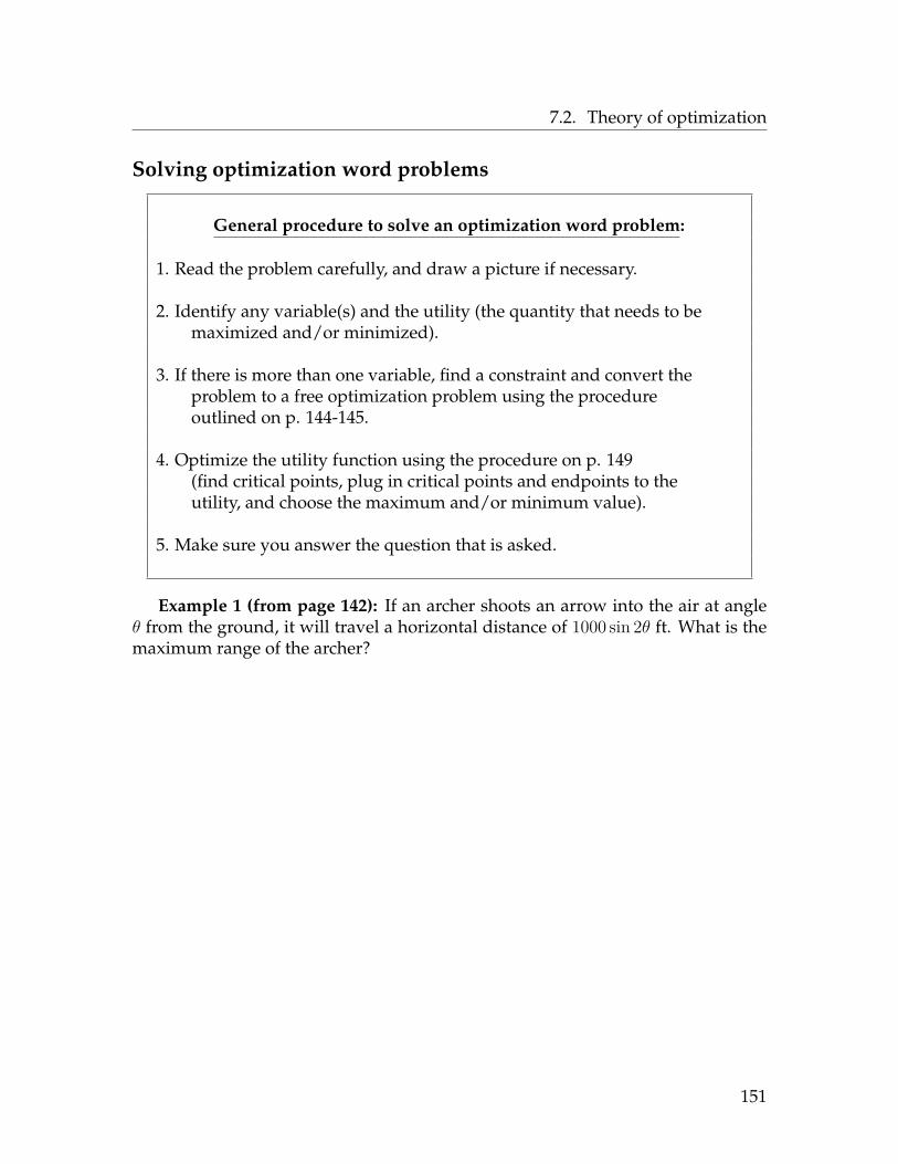
7.2. Theory of optimization
Solving optimization word problems
General procedure to solve an optimization word problem:
1. Read the problem carefully, and draw a picture if necessary.
2. Identify any variable(s) and the utility (the quantity that needs to bemaximized and/or minimized).
3. If there is more than one variable, find a constraint and convert theproblem to a free optimization problem using the procedureoutlined on p. 144-145.
4. Optimize the utility function using the procedure on p. 149(find critical points, plug in critical points and endpoints to theutility, and choose the maximum and/or minimum value).
5. Make sure you answer the question that is asked.
Example 1 (from page 142): If an archer shoots an arrow into the air at angleθ from the ground, it will travel a horizontal distance of 1000 sin 2θ ft. What is themaximum range of the archer?
151

7.2. Theory of optimization
Example 4 (from page 142): A farmer has 50 feet of fence with which to build arectangular pen. What dimensions of the pen make its area as big as possible?
Example 5 (from page 143): A box with a square base and no top is to be con-structed from plywood. If there is 48 square feet of plywood available, and if thelength, width and height of the box must be at least 1 foot, what is the largestvolume of a box that can be made?
152

7.2. Theory of optimization
Example 2 (from page 142): An epidemic spreads through a population in sucha way that the number of infected people, I , is a function of the number of suscep-tible people, x, by the formula
I(x) = 4 ln(x
30
)− x+ 30.
What is the maximum number of people who will become infected?
153

7.3. Graphical analysis using derivatives
7.3 Graphical analysis using derivativesTone
-4 -1 2
Definition 7.6 1. A function f is called increasing on an open interval if for anyx1 and x2 in that interval,
x1 ≤ x2 implies f(x1) ≤ f(x2).
2. A function f is called decreasing on an open interval if for any x1 and x2 inthat interval,
x1 ≤ x2 implies f(x1) ≥ f(x2).
3. A function f is called monotone on an open interval if it is either increasing ordecreasing on that interval.
Note: Constant functions are both increasing and decreasing.
Note: Functions are always said to increase or decrease on an open interval, notat a point.
154
7.3. Graphical analysis using derivatives
Theorem 7.7 (Monotonicity Test) If f is differentiable on (a, b), then
1. f ′(x) > 0 on (a, b)⇒ f is increasing;
2. f ′(x) < 0 on (a, b)⇒ f is decreasing.
Example: Determine whether or not the function f(x) = lnxx
is increasing ordecreasing on the interval (0, 1). Determine whether or not f is increasing or de-creasing on the interval (4, 5).
Solution: Whether or not the function is increasing or decreasing depends onwhether the derivative f ′(x) is positive or negative. By the Quotient Rule,
f ′(x) =1x· x− 1 · ln x
x2 = 1− ln xx2 .
When x ∈ (0, 1),
When x ∈ (4, 5),
Concavity
Definition 7.8 Let f : R→ R be a function.
1. f is called concave up on an open interval if f ′ is increasing on that interval.
2. f is called concave down on an open interval if f ′ is decreasing on that inter-val.
3. A number c is called an inflection point of f if the concavity of f changes at c.
155
7.3. Graphical analysis using derivatives
Theorem 7.9 (Concavity Test) Let f be a function so that f ′′ exists on (a, b). Then:
1. if f ′′(x) > 0 for all x ∈ (a, b), then f is concave up on (a, b);
2. if f ′′(x) < 0 for all x ∈ (a, b), then f is concave down on (a, b).
3. c is an inflection point of f if and only if the sign of f ′′ changes at c.
Remark: Based on the discussion from Chapter 5, if a function is concave upat/near x, then it will lie above the tangent line at x. If a function is concave downat/near x, then it will lie below the tangent line at x. If the function crosses itstangent line at x, then x is an inflection point of f .
Example: Determine whether the function f(x) = x2e−x is concave up or con-cave down on the interval (1, 2).
Solution: By the Product and Chain Rules,
f ′(x) = 2xe−x − x2e−x
and
f ′′(x) = [2e−x − 2xe−x]− [2xe−x − x2e−x] = 2e−x − 4xe−x + x2e−x
= e−x(2− 4x+ x2)
When x ∈ (1, 2),
156

7.3. Graphical analysis using derivatives
Example: Find the inflection points of the function f(x) = x3 + 3x2 − 2x+ 1.
Solution: Compute the second derivative of f :
f ′(x) = 3x2 + 6x− 2
f ′′(x) = 6x+ 6
The second derivative can also be used to classify critical points as local maximaor local minima using the following test:
Theorem 7.10 (Second Derivative Test) Suppose f ′(c) = 0 and that f ′′ is contin-uous on an open interval containing c. Then:
1. if f ′′(c) > 0, then f has a local minimum at c;
2. if f ′′(c) < 0, then f has a local maximum at c;
3. if f ′′(c) = 0, then this test is inconclusive.
More sophisticated ideas along the lines of the Second Derivative Test weredeveloped in your lab assignment on applications of derivatives. These ideas aresummarized in this theorem:
Theorem 7.11 (nth Derivative Test) Suppose f is continuous on an open intervalcontaining c and f ′(c) = f ′′(c) = f ′′′(c) = ...f (n−1)(c) = 0 but f (n)(c) 6= 0. Then:
1. if n is even and f (n)(c) > 0, then f has a local minimum at c;
2. if n is even and f (n)(c) < 0, then f has a local maximum at c;
3. if n is odd, then f has no local extremum at c.
Before the days of Mathematica and graphics calculators, this is how peoplelearned to sketch the graphs of functions. In 2014, it is more useful to use theseideas to study applied optimization problems.
157

7.3. Graphical analysis using derivatives
Returning to Example 2 (from long ago): An epidemic spreads through a pop-ulation in such a way that the number of infected people, I , is a function of thenumber of susceptible people, x, by the formula
I(x) = 4 ln(x
30
)− x+ 30.
What is the maximum number of people who will become infected?
Recall that we said our goal was to maximize I(x) on (0,∞). We found earlierthat
I ′(x) = 4x− 1
and therefore the critical points of I are
x = 0 (where I ′(x) DNE);
x = 4 (where I ′(x) = 0).
To determine whether or not x = 4 is the location of an extremum, we can usesome analysis from this section:
I ′′(x) = −4x2 ⇒ I ′′(4) = −4
42 = −14 < 0
158
7.4. More examples of optimization problems
7.4 More examples of optimization problemsExample 6: A farmer grows zucchini. He has 10 acres available to plant; if he
plants x acres his profit/loss will be 2x3 − 33x2 + 108x dollars. How many acresshould the farmer plant (assuming he wants to make as much money as possible)?
159

7.4. More examples of optimization problems
Example 7: In the human body, arteries must branch repeatedly to deliverblood to the entire body. Suppose a small artery branches off from a large artery atangle θ; the energy lost due to friction in this setting is approximately
E = csc θ + 1− cot θ16 .
Find the value of θ that minimizes the energy loss.
160

7.4. More examples of optimization problems
Example 8: A 12” by 12” square sheet of cardboard is made into an open box(i.e. no top) by cutting squares of equal size out of each corner and folding up thesides along the dotted lines (see the pictures below). Find the dimensions of thebox with the largest volume.
161
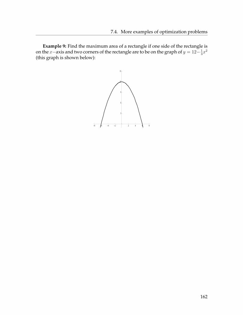
7.4. More examples of optimization problems
Example 9: Find the maximum area of a rectangle if one side of the rectangle ison the x−axis and two corners of the rectangle are to be on the graph of y = 12− 1
3x2
(this graph is shown below):
-8 -6 -4 -2 2 4 6 8
3
6
9
12
15
162

7.4. More examples of optimization problems
Example 10: Michigan wants to build a new stretch of highway to link two siteson either side of a river (see the picture below) which is 2 miles wide. The secondsite is 12 miles downriver from the first site. It costs the state $13 million per mileto build over water and $5 million per mile to build over land. How should thestate build its road to minimize costs?
River
� - y12 mi CITY 2
yCITY 1
2 mi
Solution: First, it only makes sense to build a bridge in a straight line over theriver, then to build along the riverbank to the other city. So the road goes along thesolid lines shown below:
yy
2
x12− x
√4 + x2
@@@
@@
Letting x be as indicated in the picture, that means the cost of the road is
C(x) = cost of road along shore + cost of bridge
= 5(12− x) + 13√
4 + x2.
Our goal is to maximize this utility on the interval [0, 12]. First, differentiate (usethe Chain Rule on the second term):
C ′(x) = −5x+ 13√4 + x2
· (2x) = −5x+ 13x√4 + x2
.
Set this equal to zero and solve for x (details omitted, ask me if you don’t followthis):
0 = −5x+ 13x√4 + x2
⇒ 5x = 13x√4 + x2
⇒ x = 0, x = 56
Plug the endpoints x = 0 and x = 12 and the critical point x = 56 into the utility
C; you will find that the minimum value of C is when x = 56 . Therefore the state
should angle the bridge so that it goes 5/6 mile downastream as it crosses the river.
163

7.5. Homework exercises
7.5 Homework exercisesIn Problems 1-6, you are given a word problem. Identify the utility and write
the utility as a function of one variable. (You do not need to actually solve theproblem.)
1. Find the maximum product of two numbers whose sum is 12.
2. On a given day, the rate of traffic flow on a conjested roadway is given byF (v) = v
24+.01v2 , where v is the velocity of the traffic. Find the velocity whichmaximizes the rate of traffic flow.
3. A farmer will build a rectangular pen, where one side of the pen is against ariver (and does not need to be fenced). If he wants the pen to enclose an areaof 3 acres, what is the minimum amount of fence that he can use?
4. Find the maximum sum of two numbers, where the second number is threetimes the reciprocal of the first.
5. A box has a square base. Find the maximum volume of the box, if the sur-face area of the box is 300 square units (assume that the box has a top and abottom).
6. The potential energy of a particle moving along an axis (say the x−axis) isE = b
(a2
x2 − ax
)where a, b are positive constants and x > 0. What value of x
minimizes this potential energy?
In Problems 7-12, you are given a graph of some unknown function. In eachpicture, you should assume the graph continues to the left and right (i.e. that theextreme left and right ends of the graph have arrows on them). For each function:
(a) Give the location of any local minima of f ;(b) Find the global minimum value of f on the interval [−1, 4];(c) Give the location of any local maxima of f ;(d) Find the global maximum value of f on the interval [−1, 4].
7.
-5 -4 -3 -2 -1 1 2 3 4 5
-5
-4
-3
-2
-1
1
2
3
4
5
8.
-5 -4 -3 -2 -1 1 2 3 4 5
-5
-4
-3
-2
-1
1
2
3
4
5
164

7.5. Homework exercises
9.
-5 -4 -3 -2 -1 1 2 3 4 5
-5
-4
-3
-2
-1
1
2
3
4
5
10.
-5 -4 -3 -2 -1 1 2 3 4 5
-5
-4
-3
-2
-1
1
2
3
4
5
11.
-5 -4 -3 -2 -1 1 2 3 4 5
-5
-4
-3
-2
-1
1
2
3
4
5
12.
-5 -4 -3 -2 -1 1 2 3 4 5
-5
-4
-3
-2
-1
1
2
3
4
5
In Problems 13-20, find all critical points of the given function.
13. f(x) = x2(x2 − 4)
14. f(x) = 3x1/5 + 2
15. f(x) = x3 − 3x+ 4
16. f(x) = |x|
Hint: consider the graph of f .
17. f(x) = 4e−x
18. f(x) = x7/3 − 28x1/3
19. f(x) = 3xx2−1
20. f(x) = sin x+ cosxHint: in #20, find only the criticalpoints between 0 and 2π.
21. Show that the functions f(x) and ef(x) have the same set of critical points.
165

7.5. Homework exercises
In Problems 22-31, find the absolute extrema of the given function on the indi-cated interval.
22. f(x) = sin x+ cosx on [0, 2π]
23. f(x) = x2/3 on [−1, 27]
24. f(x) = x3 − 12x+ 4 on [−3, 5]
25. f(x) = x3 − 12x+ 4 on [−3, 0]
26. f(x) = 12e−x2 on [−4, 4]
27. f(x) = 5 on [−3, 4]
28. f(x) = xx−2 on [3, 5]
29. f(x) = 3xx2−1 on [0, 2]
30. f(x) = 5− x on [1, 4]
31. f(x) = arctan(x2) on [0, 1]
32. If a person eats n sausages, then they will get heartburn in the amount ofh(n) = −n3 + 12n. If a person has the most amount of heartburn possiblefrom eating sausages, how many sausages do they eat?
33. A farmer has 96 feet of fence with which to build a rectangular pen dividedinto two pieces as follows:
What dimensions should the farmer use to build her pen, if she wants theenclosed area to be as big as possible?
34. In an endurance contest, athletes start 2 miles out to sea need to reach a lo-cation which is 2 miles inland and three miles east of their initial location(assume the seashore runs east-west). If an athlete can run 10 miles per hourand swim 5 miles per hour, what is the minimum amount of time she willneed to reach the finish? (Use Mathematica to compute the derivative of yourutility function, then use the NSolve command in Mathematica to solve for thecritical point.)
35. Suppose that if a company spends x hundred dollars on advertising, thentheir profit will be P (x) = −3x3 + 225x2 − 3600x+ 18000. How much shouldthe company spend on advertising if they want to maximize their profit, as-suming that they only have enough capital to spend $3000 on advertising?
36. A box is made with a square base and no top. If the surface area of the box is80 square units, what is the largest possible volume of the box?
166

7.5. Homework exercises
In Problems 37-40, you are given a function f and an interval (a, b). Determineif f is monotone on (a, b). If it is, determine whether f is increasing or decreasingon (a, b).
37. f(x) = x2 + 1x2 on (0, 1)
38. f(x) = ex − e−x on (−1, 1)
39. f(x) = −2x3 + 3x2 − 5 on (2, 3)
40. f(x) = ln(x+ 1x) on (0, 1)
In Problems 41-45, find all the local extrema of the given function, and classifythem as local maxima or local minima.
41. y = x4 + 4x3 + 4x2 − 3
42. f(x) = x ln x
43. f(x) = x2 − 16x
44. f(x) = e1/x2
45. f(x) = x+ 1x
In Problems 46-49, you are given a function f and an interval (a, b). Determineif f is concave up on (a, b), or concave down on (a, b).
46. f(x) = ex + e−x on (−∞,∞)
47. f(x) = x4 − 16x3 + 5 on (6, 7)
48. f(x) = −5 sin x on (π2 , π)
49. f(x) = ln(x+ 1x) on (0, 1)
In Problems 50-54, find all inflection points of the function.
50. f(x) = x3 − 3x2 + 4x− 1
51. f(x) = x+ 1x
52. f(x) = xe−2x
53. f(x) = x2 + 2x+ 3
54. f(x) = sin x− cosx(Hint: in #54, only find the inflectionpoints between 0 and 2π)
55. Suppose f is some function such that f ′(2) = f ′′(2) = f ′′′(2) = 0 and f (4)(2) =−3. Is x = 2 the location of a local maximum, local minimum, or neither?
56. Suppose f is some function such that f ′(4) = f ′′(4) = f ′′′(4) = ... = f (14)(4) =0 and f (15)(4) = 2. Is x = 4 the location of a local maximum, local minimum,or neither?
57. Suppose f is some function such that f ′(−1) = f ′′(−1) = f ′′′(−1) = ... =f (11)(−1) = 0 and f (12)(−1) = −5. Is x = −1 the location of a local maximum,local minimum, or neither?
58. Suppose f is some function such that f ′(0) = f ′′(0) = f ′′′(0) = ... = f (100)(0) =0 and f (101)(0) = −17. Is x = 0 the location of a local maximum, local mini-mum, or neither?
167

7.5. Homework exercises
59. Suppose f is some function such that f ′(4) = f ′′(4) = f ′′′(4) = ... = f (99)(4) =0 and f (100)(4) = 2
3 . Is x = 4 the location of a local maximum, local minimum,or neither?
60. Let f(x) = x2
x2+1 for x > 0. Determine where the graph of f is steepest (i.e.where the slope of the graph is a maximum).
61. The Gompertz growth curve, whose formula is
W (t) = ae−be−t,
is useful in several fields (including biology and economics). Assuming aand b are positive constants, find the value of t at which the rate of change ofW (t) with respect to t is largest.
62. Suppose that a worker can make Q(t) = −t3 + 12t2 + 60t items in t hours.
a) Explain why the efficiency of the worker at time t can be measured byQ′(t).
b) Find the time at which the worker is most efficient.
63. A rectangular poster is to be made which consists of a printed region and anunprinted margin, which is 3 inches on the top and bottom but 2 inches onthe left and right side. If the total area of the poster is to be 120 square inches,what dimensions of the poster maximize the area of the printed region?
64. Suppose a wire of length 4 ft is cut into two pieces. Each piece is bent to forma square; find the largest possible combined area from the two pieces.
65. The velocity of air moving through a person’s windpipe is V (r) = Cr2(A−r)for constants C and A, where r is the radius of the windpipe.
a) Find the radius which maximizes this velocity.
b) Suppose that normally, a person’s windpipe has radius A. When a per-son coughs, the windpipe changes radius so that air moves through thewindpipe as quickly as possible. Based on your answer to (a), does aperson’s windpipe get wider or narrower when a person coughs?
66. Find the point on the curve y = x2 which is closest to the point (2, 0). Hint:Don’t minimize the distance to the point; minimize the square of the distanceto the point.
67. To transmit data (like a music file) electronically, the file has to be translatedinto a sequence of 0s and 1s so that it can be read by a computer or phone.An important computation related to the coding of files by 0s and 1s is the
168

7.5. Homework exercises
computation of a quantity called entropy, which is given by the followingformula:
h(x) = x ln x+ (1− x) ln(1− x)
Find the value of x ∈ (0, 1) which maximizes the entropy h.
Answers
1. Utility is the product denoted by U(x) = x(12− x).
2. Utility is the rate of traffic flow denoted by F (v) = v24+.01v2 .
3. Utility is the amount of fence used, denoted byA(x) = x+ 6x
orA(x) = 2x+ 3x,
depending on your setup.
4. Utility is the sum of the numbers, denoted by U(x) = x+ 3x.
5. Utility is the volume of the box, denoted by V (x) = x2 · 300−2x2
4x .
6. Utility is the energy, denoted by E(x) = b(a2
x2 − ax
).
7. a) x = −4, x = 0, x = 3.5b) −2.2c) x = −1.2, x = 1.4d) .4
8. a) all x are local mins
b) 3c) all x are local maxs
d) 3
9. a) x = −3b) −1.2c) no local max
d) 5
10. a) x = −1b) 0c) no local max
d) no absolute max
11. a) x = 2
b) −2c) x = −2d) no absolute max
12. a) x = 2b) −2c) x = −2d) 3
13. x = 0, x =√
2, x = −√
2
14. x = 0
15. x = 1, x = −1
16. x = 0
17. None
18. x = 0, x = 2, x = −2
19. x = 1, x = −1
20. x = π4 ,
5π4
169

7.5. Homework exercises
21. Let g(x) = ef(x). By the Chain Rule, the derivative of g is g′(x) = ef(x)f ′(x).Since ef(x) always exists and is never zero, g′(x) = 0 only if f ′(x) = 0 and g′(x)DNE only if f ′(x) DNE. Thus g(x) and f(x) have the same critical points.
22. Max is√
2 at π/4; min is −√
2 at 5π/4
23. Max is 9 at x = 27; min is 0 at x = 0
24. Max is 69 at x = 5; min is −12 at x = 2
25. Max is 20 at x = −2; min is 4 at x = 0
26. Max is 12 at x = 0; min is 1
2e−16 at x = ±4
27. Max and min are 5 occuring at all x
28. Max is 3 at x = 3; min is 53 at x = 5
29. No max or min because of the asymptote at x = 1
30. Max is 4 at x = 1; min is 1 at x = 4
31. Max is π4 at x = 1; min is 0 at x = 0
32. 2 sausages
33. Relative to the picture in the homework assignment, the height should be 16feet and the width (all the way across) should be 24 feet.
34. .728134 hours
35. $3000
36. 160√
53 cubic units.
37. Decreasing on (0, 1)
38. Increasing on (−1, 1)
39. Decreasing on (2, 3)
40. Decreasing on (0, 1)
41. x = 0 local min;
x = −1 local max;
x = −2 local min
42. x = 1e
local min
43. x = −2 local min
44. No local extrema
45. x = −1 local max; x = 1 local min
46. Concave up on (−∞,∞)
47. Concave down on (6, 7)
48. Concave up on (π2 , π)
49. Concave up on (0, 1)
50. x = 1
170

7.5. Homework exercises
51. None
52. x = 1
53. None
54. x = π4 ; x = 5π
4
55. local maximum
56. neither
57. local maximum
58. neither
59. local minimum
60. The graph is steepest at x = 1√3 .
61. At t = ln b.
62. a) The efficiency of the worker is the rate at which the worker makes items;this rate is given by the derivative Q′(t).
b) At t = 4.
63. The width should be 4√
5 inches and the height should be 6√
5 inches.
64. 1 sq ft. (Cut the wire into a piece of length 4 ft and a piece of length 0 ft.)
65. a) r = 2A/3.
b) It gets narrower, since 2A/3 is less than A.
66. (.835, .697) (solve for the critical point using Mathematica)
67. x = 12
171

Chapter 8
Other Applications ofDifferentiation
8.1 Tangent line and quadratic approximationMotivation: Suppose you wanted to estimate
√102 without the use of a calcu-
lator. (Put another way, how does your calculator produce an approximation of√102? )
A way of rephrasing this is as follows: let f(x) =√x. What is the approximate
value of f(102)?
What we know is that f(100) =√
100 = 10, and since 102 is a little bit biggerthan 100,
√102 should be a bit bigger than 10. But how much bigger?
To address this issue, we use the ideas of calculus. Recall from Chapter 4 thatthe tangent line to a function at x = 100 is the line which most closely approximatesthe function at values near 100. Let’s give a name to the tangent line at 100 and callit L.
10 20 30 40 50 60 70 80 90 100 110 120 130 140 150 160 170 180 190 200
1
2
3
4
5
6
7
8
9
10
11
12
13
14
15
99. 99.5 100. 100.5 101. 101.5 102. 102.5 103.
9.9
10.
10.1
172
8.1. Tangent line and quadratic approximation
Now from a calculation we did on page 83 of these notes, we found that thetangent line to a function f at a is
L(x) = f(a) + f ′(a)(x− a).
In our setting, f(x) =√x so f ′(x) = 1
2√x
and a = 100. So we have
L(x) = f(a) + f ′(a)(x− a)= f(100) + f ′(100)(x− 100)
=√
100 + 12√
100(x− 100)
= 10 + 120(x− 100).
The whole point of this is that the tangent line closely approximates the originalfunction, so
√102 = f(102) ≈ L(102) = 10 + 1
20(102− 100) = 10 + 220 = 10.1.
Note: the actual value of√
102 is 10.0995... so our approximation of 10.1 is correctto four decimal places.
Definition 8.1 (Linear approximation) Given a differentiable function f and a num-ber a at which you can easily compute f(a) and f ′(a), the values f(x) for x close to acan be estimated by the formula
f(x) ≈ L(x) = f(a) + f ′(a)(x− a).
This procedure is called tangent line approximation or linear approximation.
The function L(x) described above (which depends on f and a) has lots ofnames. It is also denoted P1(x) and is called:
1. the tangent line to f at a;2. the linearization of f at a;3. the standard linear approximation to f at a; and4. the first Taylor polynomial of f centered at a.
173
8.1. Tangent line and quadratic approximation
Example 1: Estimate 4√
17 using tangent line approximation.
Note: You do not need to know the formula for f to perform a tangent lineapproximation. All you need to know are the values of f(a) and f ′(a) (these twonumbers can often be determined experimentally if f is some unknown functiondealing with some experiment).
Example 2: A biologist is growing bacteria in a petri dish. At 2:00 PM, sheestimates that there are 20000 living bacteria in the dish, and that the number ofbacteria is growing at a rate of 500 bacteria per minute. Use tangent line approxi-mation to estimate the number of bacteria in the dish at 2:05 PM.
A more interesting calculus problem: In the example above will the answeroverestimate, or underestimate the number of bacteria that are actually in the dish?
174

8.1. Tangent line and quadratic approximation
0 5time
20000
22500
ð of bacteria
To get a better approximation which accounts for this kind of error, we approx-imate f not by a line but by a parabola which has the same slope and concavity asf at a:
Definition 8.2 (Quadratic approximation) Given a twice-differentiable functionf and a number a at which you can easily compute f(a), f ′(a) and f ′′(a), the val-ues f(x) for x close to a can be approximated by the formula
f(x) ≈ Q(x) = f(a) + f ′(a)(x− a) + 12f′′(a)(x− a)2.
This procedure is called quadratic approximation.
In general, quadratic approximation of a function is more accurate than lin-ear approximation. In Math 230, you will learn how to approximate functions fby polynomials of larger degree which can produce highly accurate estimates toproblems.
The function Q(x) described above (which depends on f and a) also has lots ofnames. It is also denoted P2(x) and is called:
1. parabolic approximation to f at a;2. the standard quadratic approximation to f at a; and3. the second Taylor polynomial of f at a.
175

8.1. Tangent line and quadratic approximation
Example 3: Approximate√
102 using quadratic approximation.
Example 4: Suppose the biologist in Example 2 assumes (in addition to whatshe knew in Example 2) that the number of bacteria in her petri dish at time t isgiven by a function whose second derivative at 2:00 PM is 10. Estimate the numberof bacteria in her dish at 2:15 PM using quadratic approximation.
176

8.1. Tangent line and quadratic approximation
Differentials
We will now establish some additional notation which will be used later in thecourse. Given a function y = f(x), we create a new function with 2 inputs and oneoutput. The two inputs are:
x = an “initial” value of xdx = a change in the value of x
Thus, we think of x as changing from x to x + dx. Given these inputs, we de-fine dy to be the estimated change in y that we would compute using tangent lineapproximation at x:
dy = L(x+ dx)− L(x)= [f(x) + f ′(x)(x+ dx− x)]− [f(x) + f ′(x)(x− x)]= [f(x) + f ′(x) dx]− [f(x)]= f ′(x) dx.
The quantities dy and dx are called differentials. They represent small changes in yand x, respectively and are related by the formula
dy = f ′(x) dx
.
Example: Suppose y = 2x6 + sin x− 3. Compute dy (in terms of x and dx).
177

8.2. L’Hôpital’s rule
A picture associated to differentials:
x x+Dx
fHxL
fHx+DxL
In principle dy ≈ the actual change in y, since L(x) ≈ f(x).
8.2 L’Hôpital’s ruleRecall that most limits are evaluated by “plugging in”, i.e.
limx→5
2x+ 1x− 3 = 2(5) + 1
5− 3 = 112 .
Other limits are not so easy:
limx→2
x2 − 4x− 2
limx→0
sin xx
178

8.2. L’Hôpital’s rule
The 00 obtained by plugging in 2 to the expression x2−4
x−2 or by plugging in 0 tosinxx
is called an “indeterminate form”. Note that both examples above are of theform 0
0 , but evaluate to different answers. More generally:
Definition 8.3 An indeterminate form is an expression which can work out to oneof many different answers, depending on the context.
Examples of indeterminate forms:
00
∞∞
0 · ∞ ∞−∞ 1∞ ∞0 00
Forms which are not indeterminate:
0nonzero constant
= 0 nonzero constant0 = ±∞
∞0 = ±∞ 0
∞= 0 0 · 0 = 0 01 = 0 10 = 1
(nonzero constant)0 = 1 ∞nonzero constant
= ±∞ nonzero constant∞
= 0
Methods we have already learned (in Chapter 3) to evaluate indeterminateforms in limits include
•
•
•
•
One additional, and very useful, method to evaluate indeterminate forms in limitsis called L’Hôpital’s Rule:
179

8.2. L’Hôpital’s rule
Theorem 8.4 (L’Hôpital’s Rule) Suppose f and g are differentiable functions. Sup-pose also that either
limx→a
f(x) = limx→a
g(x) = 0
orlimx→a
f(x) = limx→a
g(x) = ±∞.
Then:limx→a
f(x)g(x)
L= limx→a
f ′(x)g′(x) .
Application: Expressions like 00 or ∞∞ can often be evaluated by taking deriva-
tives of the top and bottom independently, then plugging in a.
WARNING: We are not differentiating fg
here. To do this, use the quotient rule(but that has nothing to do with the evaluation of the limit).
WARNING: Be sure that the limit you are calculating is a common (i.e. easy)indeterminate form before using L’Hôpital’s Rule.
Notation: The symbol L= is used to denote usage of L’Hôpital’s Rule. It is justan equals sign, and the L tells the reader that you are using L’Hôpital’s Rule.
Example 1:
limx→2
x2 − 4x− 2
Example 2:
limx→0
sin xx
180
8.2. L’Hôpital’s rule
Example 3:
limx→0
3x2
Example 4:
limx→3
x− 32x+ 1
Example 5:
limx→∞
7 + 2x2
x2 − 3x+ 1
Example 6:
limx→0
cosx− 1x2
181

8.2. L’Hôpital’s rule
Example 7:
limx→∞
x2
x+ 1
Example 8: Evaluate this limit, where n is a positive integer:
limx→∞
xn
ex
You can also evaluate other indeterminate forms (like 0 ·∞,∞−∞, 1∞,∞0, 00)by first doing some algebra, then using L’Hôpital’s Rule:
Example 9:
limx→∞
x sin(1x
)
182

8.2. L’Hôpital’s rule
Example 10:
limx→0+
(cscx− cotx)
Example 11:
limx→∞
(1 + 1
x
)xNote: The answer to this problem should be memorized.
183
8.2. L’Hôpital’s rule
WARNING: L’Hôpital’s Rule is a dangerous thing to rely on too much for tworeasons:
(1)
Example 12:
limx→0
cosx− 1 + 12x
2
ex − 1− x− 12x
2 − 16x
3
(2)
Example 13:
limx→∞
√x2 + 1x
184

8.3. Newton’s method
8.3 Newton’s methodGoal: use calculus to quickly and accurately approximate solutions to equa-
tions.
First, to solve any equation in one variable, it is sufficient to solve equationswhere one side is equal to zero (i.e. to find roots a.k.a. x-intercepts of functions).This is because if you are given an equation of the form
g(x) = h(x)
you can rewrite it as
g(x)− h(x) = 0 or h(x)− g(x) = 0.
So our goal is: given function f , find (or at least approximate) r such that f(r) =0. The procedure we will use is called Newton’s method and works as follows:
1. Guess the value of r. Call yourguess x0 (x0 is called the “initialguess” or “seed”).
2. Draw the tangent line to f at x0.
3. Find the x−intercept of the tan-gent line from step (2). Call thisx−int x1.
(Ideally, x1 is closer to r than x0 is.)
4. Draw the tangent line to f at x1.
5. Find the x−intercept of the tan-gent line from step (2). Call thisx−int x2.
(Ideally, x2 is closer to r than x1 is.)
6. Repeat the procedure over andover: given xn, sketch the tangentline to f at xn; call this x−int of thistangent line xn+1.
7. You get a sequence of pointsx0, x1, x2, x3, ...
The numbers xn should (hope-fully) get closer and closer to r, sothey approximate r better and bet-ter as n gets larger.
185

8.3. Newton’s method
Let’s implement this procedure for an arbitrary function f and initial guess x0:
The tangent line to f at xn has equation
and xn+1, the x−intercept of this line is found as follows:
Example: Approximate a solution to x3 − x = 2 by using Newton’s methodwith initial guess 2 and two steps.
186

8.3. Newton’s method
Example: Approximate a solution to x3−x = 2 by using Newton’s method andgetting an approximation correct to 4 decimal places.
Newton’s method on Mathematica
Newton’s method is easy to implement on Mathematica. You need three lines ofcode, all in the same cell. For example, to implement Newton’s method for thefunction f(x) = x2 − 2 where x0 = 3 and you want to perform 6 iterations (to findx6), just type
f[x_] = x^2 - 2;Newton[x_] = N[x - f[x]/f’[x]];NestList[Newton, 3, 6]
and execute (all three lines at once). The first line defines the function f , the secondline gives a name to the formula you iterate in Newton’s method, and the last lineiterates the formula and spits out the results.
The resulting output for the code listed above is:
{3, 1.83333, 1.46212, 1.415, 1.41421, 1.41421, 1.41421}
These numbers are x0, x1, x2, ..., x6 so for example, x2 = 1.46212 and x4 = 1.41421...and x6 = 1.41421 (the same as x4 to 5 decimal places).
To implement Newton’s method for a different function, different initial guessand different number of iterations, simply change the formula for f , change the 3to the appropriate value of x0 and the 6 to the number of times you want to iterateNewton’s method.
187

8.3. Newton’s method
Example: Use Newton’s method to approximate the solution to
cos 2x+ 3x = sin x.
Obtain an approximation which is accurate to four decimal places.
Mathematica code:f[x_] = Cos[2x] + 3x - Sin[x];Newton[x_] = N[x - f[x]/f’[x]];NestList[Newton,-1/2,10]
output:
{-1/2, -0.373791, -0.367115, -0.367093, -0.367093, -0.367093,-0.367093, -0.367093, -0.367093, -0.367093, -0.367093 }
Potential problems with Newton’s method
Example 1: Use Newton’s method to find a solution of
x1/3 = 0
using initial guess x = 1.
-10 -5 5 10
-4
-2
2
4
188
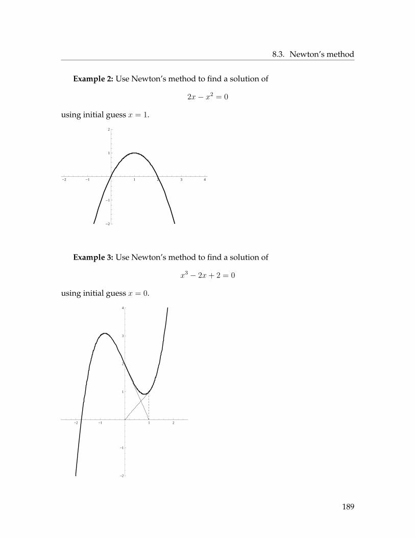
8.3. Newton’s method
Example 2: Use Newton’s method to find a solution of
2x− x2 = 0
using initial guess x = 1.
-2 -1 1 2 3 4
-2
-1
1
2
Example 3: Use Newton’s method to find a solution of
x3 − 2x+ 2 = 0
using initial guess x = 0.
-2 -1 1 2
-2
-1
1
2
3
4
189

8.3. Newton’s method
Example 4: Here is a graph of f(x) = 12(x+ 2)(x− 3)(x− 4)(x− 5) + 4:
x1 r x0
This function has two roots, a negative one which is about −2 and a positiveone which is about 3. If you use initial guess x0 = 3.4, you get the following:
x1 = −8.9451;x2 = −6.28878;x3 = −4.38652; ... xn → −1.96114
which is the negative root. In other words, you get a root, but not the root youwanted.
To summarize: sometimes Newton’s method fails. Common reasons for thisinclude:
1. “overshooting” (as in Example 1) - caused by vertical tangency at the root
2. f ′(xn) being equal to zero for some n (as in Example 2) - caused by horizontaltangency at xn
3. periodicity in the sequence xn (as in Example 3) - caused by “poor” or “un-lucky” initial guess
4. getting an unexpected root (as in Example 4) - caused by having a pointwhere f ′(x) is small too close to the root you want
Reasons for the failure of Newton’s method can always be explained graphically.
190

8.4. Related rates
8.4 Related ratesExample: The volume of a spherical bubble is given by V = 4
3πr3 (where r is in
mm and V is in mm3). If the radius of the bubble is growing at a rate of 3 mm/sec,how fast is the volume growing when the radius is 2 mm?
This is an example of a related rates problem. Related rates problems are de-scribed as follows:
•
(In the example, the radius and the volume are changing)
•
(In the example, you are given the rate of change of the radius)
•
(In the example, you are asked to compute the rate of change of the volume)
Conceptually, the key thing about solving related rates problems is to understandthat there is a hidden variable in the problem:
Given information in the example:
To solve this problem, start with the equation relating V and r, and differentiateit with respect to t (i.e. take d
dtof both sides):
191
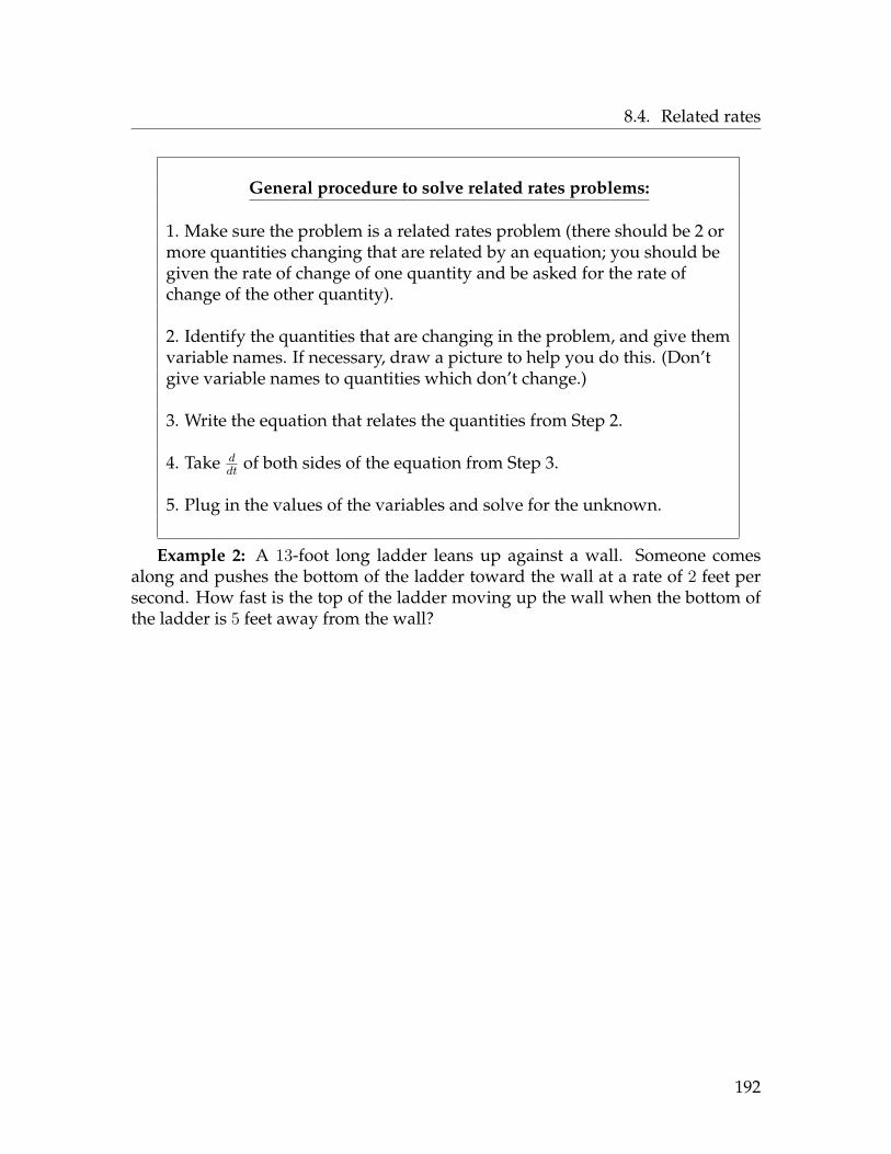
8.4. Related rates
General procedure to solve related rates problems:
1. Make sure the problem is a related rates problem (there should be 2 ormore quantities changing that are related by an equation; you should begiven the rate of change of one quantity and be asked for the rate ofchange of the other quantity).
2. Identify the quantities that are changing in the problem, and give themvariable names. If necessary, draw a picture to help you do this. (Don’tgive variable names to quantities which don’t change.)
3. Write the equation that relates the quantities from Step 2.
4. Take ddt
of both sides of the equation from Step 3.
5. Plug in the values of the variables and solve for the unknown.
Example 2: A 13-foot long ladder leans up against a wall. Someone comesalong and pushes the bottom of the ladder toward the wall at a rate of 2 feet persecond. How fast is the top of the ladder moving up the wall when the bottom ofthe ladder is 5 feet away from the wall?
192

8.4. Related rates
Example 3: A conical cup with height 12 in and radius 4 in is being filled withwater at the rate of 6π in3/sec. How fast is the water depth in the cone changingwhen the water is 6 in deep?
193

8.4. Related rates
Example 4: A wide receiver lines up 20 yards to the left of the center. He runsat a constant speed of 8 yards per second. The quarterback takes the snap, dropsback 4 yards, and stops. The receiver runs downfield for 1 sec, then turns 90◦ leftand runs toward the sideline. Let θ be the angle between the line from the centerto the quarterback and the line from the quarterback to the receiver; find how fastθ is changing 1.5 seconds after the snap.
194
8.5. Homework exercises
8.5 Homework exercisesIn Problems 1-4 below, compute the linear approximation L(x) to f at the givenvalue of a:
1. f(x) = 5√x, a = 1
2. f(x) = cot x, a = π/4
3. f(x) = sin 3x, a = π
4. f(x) = xex, a = 0
In Problems 5-8 below, compute the quadratic approximationQ(x) to f at the givenvalue of a:
5. f(x) = x2/3, a = 27
6. f(x) = 4 cosx, a = π
7. f(x) = ln(x+ 1), a = 0
8. f(x) = 3 secx, a = 0
In Problems 9-16 below, estimate the following quantities using tangent line ap-proximation:
9.√
50
10. (8.1)3
11. ln(1.3)
12. e.2
13. 3√
66
14. sin(.2)
15. arctan(1/3)
16. cos(π2 + 1/8)
17. Is the estimate you made in problem 9 an overestimate or an underestimate?Explain (without obtaining a decimal approximation to
√50 using a com-
puter or calculator).
18. Is the estimate you made in problem 10 an overestimate or an underestimate?Explain (without obtaining a decimal approximation to (8.1)3 using a com-puter or calculator).
In Problems 19-22 below, estimate the following quantities using quadratic approx-imation:
19. 173/2
20. cos 12
21. e1/3
22.√
150
195
8.5. Homework exercises
In Problems 23-26, compute dy.
23. y = 3x2 − 4
24. y = x√
1− x2
25. y = arcsin x
26. y = e3x
27. a) Compute dy if y = 12x
3, when x = 2 and dx = .1.
b) Sketch a picture representing the computation done in part (a) of thisproblem, labelling x, dx and dy appropriately.
28. a) Compute dy if y = 1− x4, when x = 1 and dx = .1.
b) Sketch a picture representing the computation done in part (a) of thisproblem, labelling x, dx and dy appropriately.
In problems 29-46, compute the indicated limit (indicating if the limit is ±∞ ordoes not exist):
29. limx→3
2x−6x2−9
30. limx→0
√4−x2−2x
31. limx→0
2ex−2x−2x2
32. limx→3
x2−2x−3x−3
33. limx→2
x2+10x+2
34. limx→0
sin 4xsin 9x
35. limx→∞
3x2−2x+12x2+3
36. limx→∞
x4
ex/3
37. limx→∞
lnxx2
38. limx→∞
ex
x9
39. limx→∞
2000x2014
ex
40. limx→2+
(8
x2−4 −xx−2
)41. lim
x→1+
(3
lnx −2
x−1
)42. lim
x→0
(1ex− 1
cosx
)43. lim
x→∞x2 tan(1/x2)
44. limx→π
2−
tanxsecx
45. limx→∞
x1/x
Hint: Follow the procedure of Exam-ple 11 on page 183.
46. limx→0
xx
47. Approximate (by hand) a solution to 2x3 + x2 − x = −1 by using Newton’smethod with initial guess x = −1 and two steps.
48. Approximate (by hand) a solution to x5 = 4 by using Newton’s method withinitial guess x = 1 and two steps.
196
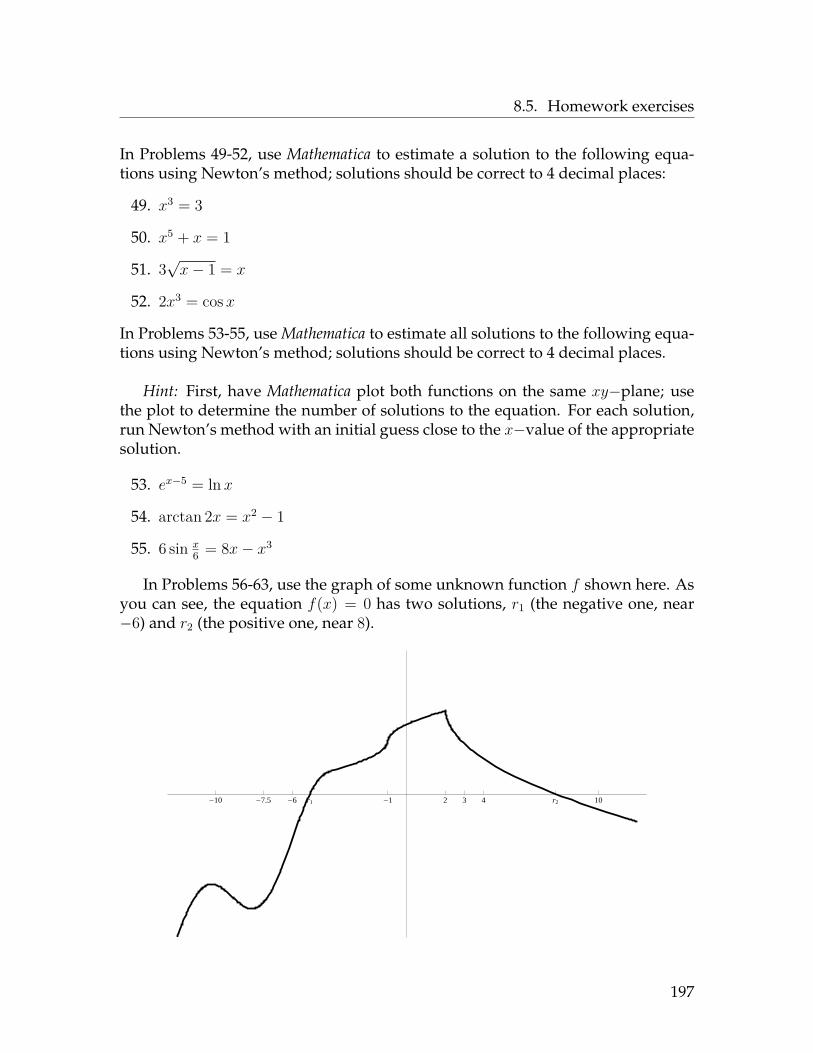
8.5. Homework exercises
In Problems 49-52, use Mathematica to estimate a solution to the following equa-tions using Newton’s method; solutions should be correct to 4 decimal places:
49. x3 = 3
50. x5 + x = 1
51. 3√x− 1 = x
52. 2x3 = cosx
In Problems 53-55, use Mathematica to estimate all solutions to the following equa-tions using Newton’s method; solutions should be correct to 4 decimal places.
Hint: First, have Mathematica plot both functions on the same xy−plane; usethe plot to determine the number of solutions to the equation. For each solution,run Newton’s method with an initial guess close to the x−value of the appropriatesolution.
53. ex−5 = ln x
54. arctan 2x = x2 − 1
55. 6 sin x6 = 8x− x3
In Problems 56-63, use the graph of some unknown function f shown here. Asyou can see, the equation f(x) = 0 has two solutions, r1 (the negative one, near−6) and r2 (the positive one, near 8).
-10 -7.5 -6 r1 -1 2 3 4 r2 10
197

8.5. Homework exercises
56. Suppose you were to execute Newton’s method for this function with initialguess x = 4. Will this produce an approximation to r1 or r2 (or will it notwork at all)? Explain.
57. Suppose you were to execute Newton’s method for this function with initialguess x = −6. Will this produce an approximation to r1 or r2 (or will it notwork at all)? Explain.
58. Suppose you were to execute Newton’s method for this function with initialguess x = −10 (assume that −10 is the x−coordinate of the “peak” of thefunction). Will this produce an approximation to r1 or r2 (or will it not workat all)? Explain.
59. Suppose you were to execute Newton’s method for this function with initialguess x = 3. Will this produce an approximation to r1 or r2 (or will it notwork at all)? Explain.
60. Suppose you were to execute Newton’s method for this function with initialguess x = −1. Will this produce an approximation to r1 or r2 (or will it notwork at all)? Explain.
61. Suppose you were to execute Newton’s method for this function with initialguess x = 2. Will this produce an approximation to r1 or r2 (or will it notwork at all)? Explain.
62. Suppose you were to execute Newton’s method for this function with initialguess x = −7.5. Will this produce an approximation to r1 or r2 (assume thatthe slope at −7.5 is a very small positive number)? Explain.
63. Suppose you were to execute Newton’s method for this function with initialguess x = 10. Will this produce an approximation to r1 or r2 (or will it notwork at all)? Explain.
64. Attempt Newton’s method on the function f(x) = 4x3 − 12x2 + 12x− 3 withinitial guess x = 3
2 . Try lots of iterations.
a) What happens?b) Sketch the graph of the function f using Mathematica and explain, via
the graph, the phenomenon you observe in part (a).
65. If every edge of a cube is expanding at a rate of 2 cm/sec, how fast is thevolume of the cube changing when each side is 12 cm long?
66. At a sand gravel plant, sand is falling off a conveyor onto a conical pile ata rate of 10 cubic feet per minute. The diameter of the base of the pile isroughly three times the altitude of the pile. At what rate is the height of thepile changing when the pile is 15 feet high?
198
8.5. Homework exercises
67. The combined electrical resistance R of R1 and R2 connected in parallel isgiven by
1R
= 1R1
+ 1R2
where R,R1 and R2 are measured in ohms. If R1 is increasing at the rate of 1ohm per minute and R2 is increasing at the rate of 1.5 ohms per minute, howfast is R changing when R1 is 50 ohms and R2 is 75 ohms?
68. An oil tanker has an accident and oil pours out of the tanker at a rate of 20 ft3
per minute. If the oil spill is in the shape of a cylinder with thickness 1120 feet,
determine the rate at which the radius of the oil spill is increasing when theradius is 500 feet.
69. A Ferris wheel is 50 ft in diameter and its center is located 30 feet above theground. If the wheel rotates once every 2 minutes, how fast is a passengerrising when she is 42.5 feet above the ground?
Hint: convert the rotational speed to radians per minute.
70. A rocket blasts off directly upward from the ground. If the height of therocket at time t (measured in the number of seconds after lift-off) is 50t2 feet,find the rate of change of the angle of elevation to an observer who is 2000 feetaway from the launch pad, 10 seconds after lift-off. (The angle of elevation ismeasured between the ground and a line from the observer to the rocket.)
71. In the same situation as Problem 70, find the rate of change of the distancefrom the rocket to the observer (at the same instant as in Problem 70).
72. As a space shuttle moves into space, an astronaut’s weight decreases. Anastronaut weighing 650 N at sea level has a weight of w = 650
(6400
6400+h
)at
h kilometers above sea level. If the shuttle is moving away from Earth at 6km/sec, at what weight is the astronaut’s weight changing when h = 1.2 km?
73. Two cars approach an intersection, one heading east toward the intersectionat 30 km per hour and one heading south toward the intersection at 40 km perhour. At what rate are the cars approaching one another when the first car is.1 km from the intersection and the other is .075 m from the intersection?
199

8.5. Homework exercises
Answers
1. L(x) = 1 + 15(x− 1)
2. L(x) = 1− 2(x− π4 )
3. L(x) = −3(x− π)
4. L(x) = x
5. Q(x) = 9 + 29(x− 27)− 1
729(x− 27)2
6. Q(x) = −4 + 2(x− π)2
7. Q(x) = x− x2
2
8. Q(x) = 3 + 32x
2
9. 9914
10. 531.2
11. .3
12. .2
13. 9724
14. .2
15. 13
16. −1/8
17. Overestimate, because f ′′(49) < 0.
18. Underestimate, because f ′′(8) > 0.
19. 224332
20. 78
21. 2518
22. 4703384
23. 6x dx
24.√
1−x2− −2x2
2√
1−x2
1−x2 dx = 1(1−x2)3/2 dx
25. 1√1−x2 dx
26. 3e3x dx
27. a) .6b) Picture should look like the one
on page 178, with the functiony = 1
2x3, x = 2 and dx = .1.
28. a) −.4.
b) Picture should look like the oneon page 178, with the functiony = 1− x4, x = 1 and dx = .1.
29. 13
30. 0
31. 1
32. 4
33. 72 (this is not indeterminate)
34. 49
35. 32
36. 0
37. 0
38. ∞
39. 0
40. −32
41. ∞
42. 0 (not indeterminate)
43. 1
44. 1
45. 1
200

8.5. Homework exercises
46. 1
47. −235189
48. 3589325600
49. 1.44225
50. .754878
51. 7.8541
52. .721406
53. 1.01884 and 5.53738
54. −.482303 and 1.49966
55. −2.65184, 0 and 2.65184
56. r2
57. r1
58. won’t work
(since tangent line at x = −10never hits x−axis)
59. r2
60. won’t work
(tangent line at x = −1is vertical)
61. won’t work (function not differen-tiable at x = 2
62. r2 (tangent line at −7.5 hits x−axisclose to r2)
63. r2
64. a) Starting with the second itera-tion, you get infinity.
b) If you sketch the picture associ-ated to Newton’s method, afterthe first iteration the tangent lineis horizontal.
65. 864 cm3/sec
66. 8405π feet per minute
67. 35 ohm per minute
68. 125π feet per minute
69. 25√
3π2 ≈ 68.018 ft / min.
70. 229 radians per sec
71. 5000√29 feet per sec
72. −.432 N/sec
73. 48 km/hour
201

Chapter 9
Theory of the Definite Integral
9.1 Motivating problems: area and displacementRecall that to define the derivative of a function, we started with a real-world
problem we wanted to solve:
Then, we approximated the solution to that problem (by finding the slope ofsome secant line):
Next, we observed how the approximation got better:
This told us how to define the answer to the problem (using a limit):
(In principle, we don’t use this definition to compute derivatives; we use ruleslike the Power Rule, Product Rule, Chain Rule, etc.)
202
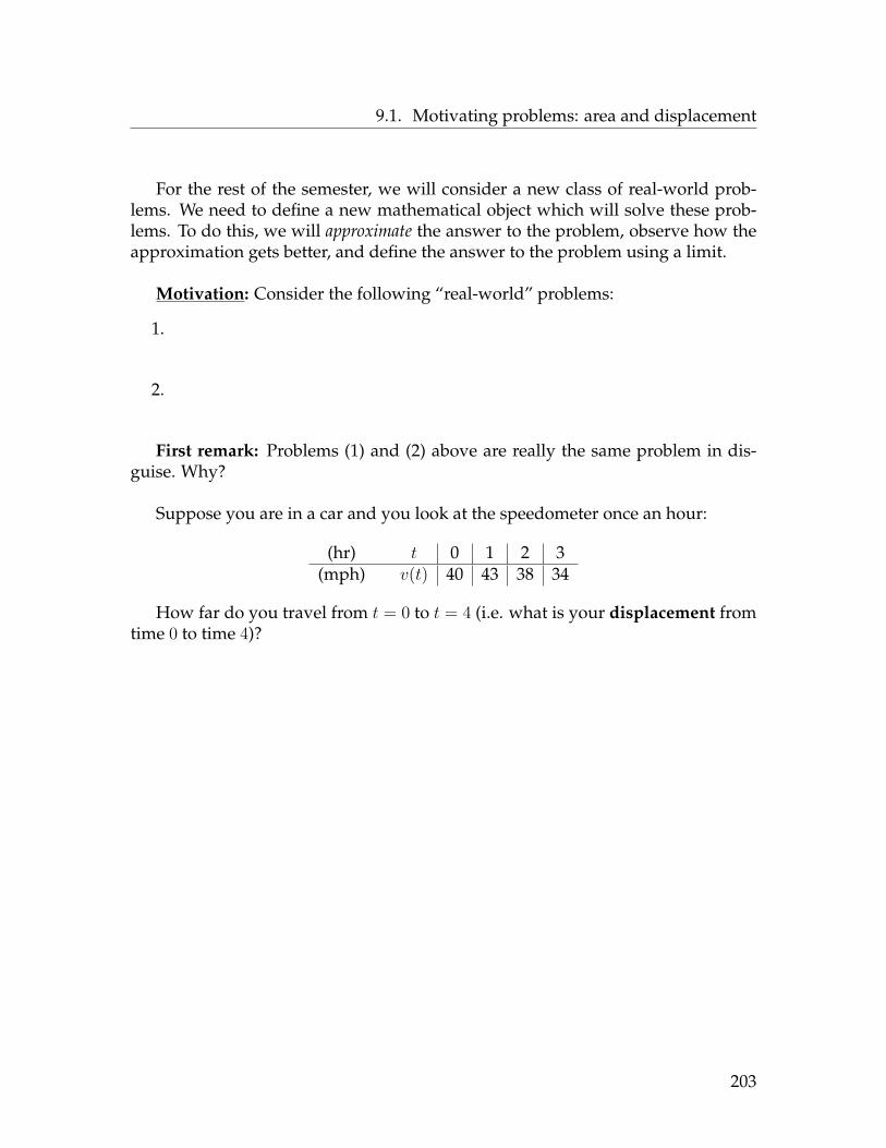
9.1. Motivating problems: area and displacement
For the rest of the semester, we will consider a new class of real-world prob-lems. We need to define a new mathematical object which will solve these prob-lems. To do this, we will approximate the answer to the problem, observe how theapproximation gets better, and define the answer to the problem using a limit.
Motivation: Consider the following “real-world” problems:
1.
2.
First remark: Problems (1) and (2) above are really the same problem in dis-guise. Why?
Suppose you are in a car and you look at the speedometer once an hour:
(hr) t 0 1 2 3(mph) v(t) 40 43 38 34
How far do you travel from t = 0 to t = 4 (i.e. what is your displacement fromtime 0 to time 4)?
203
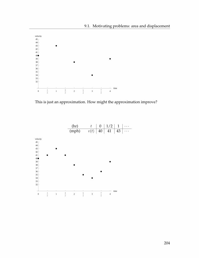
9.1. Motivating problems: area and displacement
01
21
3
22 5
23
7
24
time
32
33
34
35
36
37
38
39
40
41
42
43
44
45
velocity
This is just an approximation. How might the approximation improve?
(hr) t 0 1/2 1 · · ·(mph) v(t) 40 41 43 · · ·
01
21
3
22 5
23
7
24
time
32
33
34
35
36
37
38
39
40
41
42
43
44
45
velocity
204
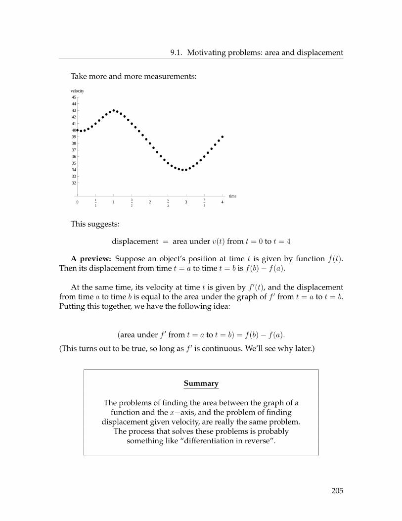
9.1. Motivating problems: area and displacement
Take more and more measurements:
01
21
3
22 5
23
7
24
time
32
33
34
35
36
37
38
39
40
41
42
43
44
45
velocity
This suggests:
displacement = area under v(t) from t = 0 to t = 4
A preview: Suppose an object’s position at time t is given by function f(t).Then its displacement from time t = a to time t = b is f(b)− f(a).
At the same time, its velocity at time t is given by f ′(t), and the displacementfrom time a to time b is equal to the area under the graph of f ′ from t = a to t = b.Putting this together, we have the following idea:
(area under f ′ from t = a to t = b) = f(b)− f(a).
(This turns out to be true, so long as f ′ is continuous. We’ll see why later.)
Summary
The problems of finding the area between the graph of afunction and the x−axis, and the problem of finding
displacement given velocity, are really the same problem.The process that solves these problems is probably
something like “differentiation in reverse”.
205
9.2. Riemann sums
9.2 Riemann sumsSummation notation
Suppose ak is some expression which can be computed in terms of k. (ak is likea(k).) For example, if ak = k2 + k, then
a1 = 12 + 1 = 2 a2 = 22 + 2 = 6 a3 = 32 + 3 = 12 etc.
Frequently in mathematics we want to add together values of ak where k rangesover some set. For example, we might want to add up
a2 + a3 + a4 + a5 + ...+ a20.
We use the following notation to represent this kind of addition:
Definition 9.1 Given numbers a1, a2, ... the sum from k = 1 to n of ak is
n∑k=1
ak = a1 + a2 + a3...+ an.
(More generally,n∑
k=mak = am + am+1 + am+2 + ...+ an.)
Example: Write the expression 32
2 + 42
2 + 52
2 + ...+ 172
2 in Σ-notation.
Example: Compute3∑
k=0
2k+1 .
206
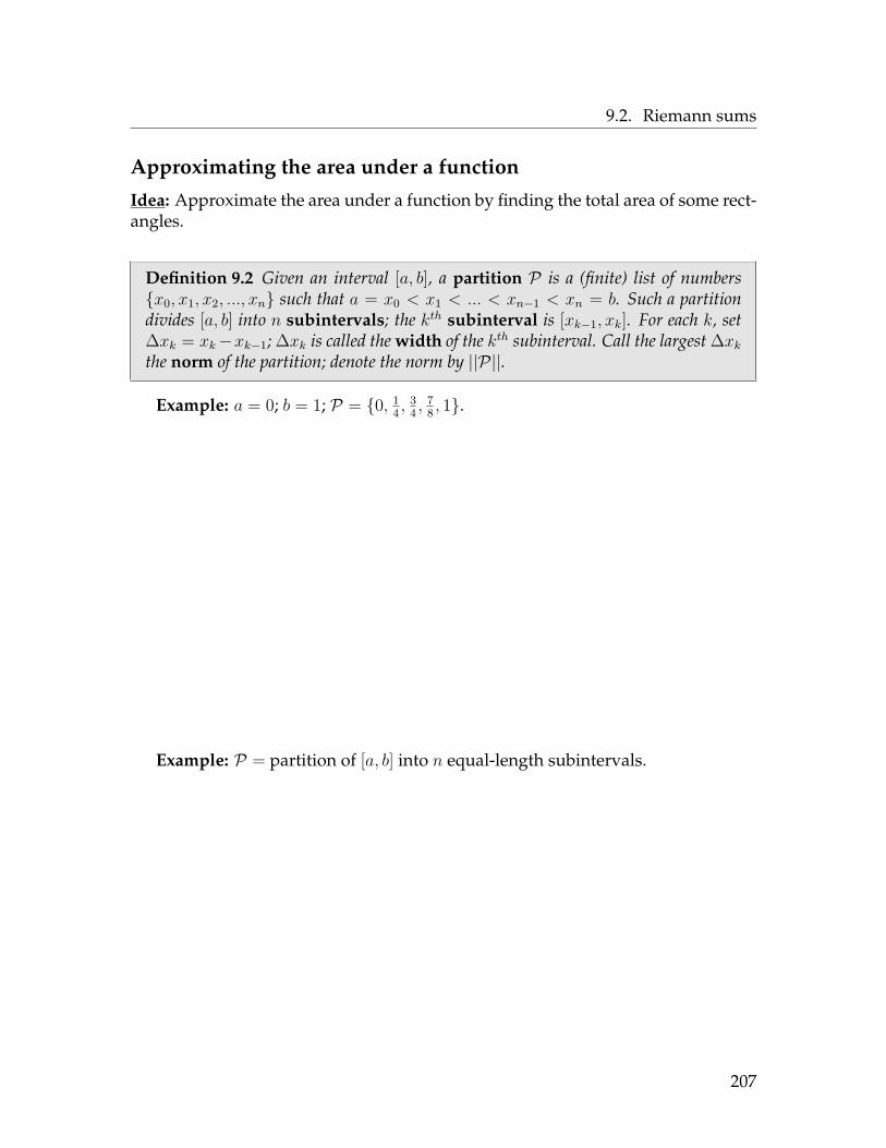
9.2. Riemann sums
Approximating the area under a function
Idea: Approximate the area under a function by finding the total area of some rect-angles.
Definition 9.2 Given an interval [a, b], a partition P is a (finite) list of numbers{x0, x1, x2, ..., xn} such that a = x0 < x1 < ... < xn−1 < xn = b. Such a partitiondivides [a, b] into n subintervals; the kth subinterval is [xk−1, xk]. For each k, set∆xk = xk−xk−1; ∆xk is called the width of the kth subinterval. Call the largest ∆xkthe norm of the partition; denote the norm by ||P||.
Example: a = 0; b = 1; P = {0, 14 ,
34 ,
78 , 1}.
Example: P = partition of [a, b] into n equal-length subintervals.
207
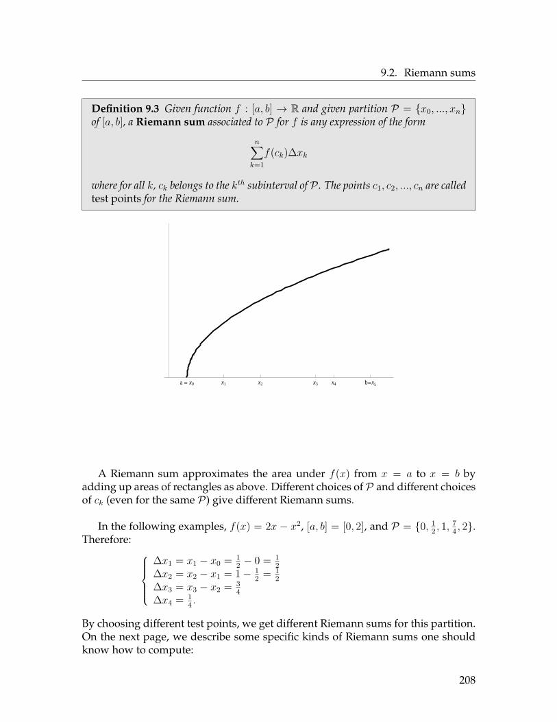
9.2. Riemann sums
Definition 9.3 Given function f : [a, b] → R and given partition P = {x0, ..., xn}of [a, b], a Riemann sum associated to P for f is any expression of the form
n∑k=1
f(ck)∆xk
where for all k, ck belongs to the kth subinterval of P . The points c1, c2, ..., cn are calledtest points for the Riemann sum.
a = x0 x1 x2 x3 x4 b=x5
A Riemann sum approximates the area under f(x) from x = a to x = b byadding up areas of rectangles as above. Different choices of P and different choicesof ck (even for the same P) give different Riemann sums.
In the following examples, f(x) = 2x − x2, [a, b] = [0, 2], and P = {0, 12 , 1,
74 , 2}.
Therefore: ∆x1 = x1 − x0 = 1
2 − 0 = 12
∆x2 = x2 − x1 = 1− 12 = 1
2∆x3 = x3 − x2 = 3
4∆x4 = 1
4 .
By choosing different test points, we get different Riemann sums for this partition.On the next page, we describe some specific kinds of Riemann sums one shouldknow how to compute:
208

9.2. Riemann sums
1. Left sum: choose ck = xk−1 = left endpoint of kth subinterval.
x0=0 x1=1�2 x2=1 x3=7�4 x4=2
1�2
3�4
1
4∑k=1
f(ck)∆xk =
2. Right sum: choose ck = xk = right endpoint of kth subinterval.
x0=0 x1=1�2 x2=1 x3=7�4 x4=2
1�2
3�4
1
4∑k=1
f(ck)∆xk =
3. Upper sum: choose ck to be the x−value corresponding to abs max of f onkth subinterval.
x0=0 x1=1�2 x2=1 x3=7�4 x4=2
1�2
3�4
1
4∑k=1
f(ck)∆xk =
4. Lower sum: choose ck to be the x−value corresponding to abs min of f onkth subinterval.
x0=0 x1=1�2 x2=1 x3=7�4 x4=2
1�2
3�4
1
4∑k=1
f(ck)∆xk =
209

9.2. Riemann sums
Note: The actual area under a function f is always greater than any lower sum,and less than any upper sum (no matter the choice of P).
Note: If f is increasing, then
Note: If f is decreasing, then
Example: Estimate the area under f(x) = x3 from x = 0 to x = 1 by using alower sum for a partition into 6 subintervals of equal length.
210

9.2. Riemann sums
Error in a Riemann sum computation
Definition 9.4 Suppose you approximate quantity Q by computing approximationA. The error in this approximation is
E = |Q− A| = |A−Q|.
Note: errors are always nonnegative.
Note: the approximation is exactly right if and only if E = 0.
Definition 9.5 Suppose you approximate quantity Q by computing approximationA. An error bound for the approximation is a number B such that the error Esatisfies E ≤ B.
Suppose you approximate an answer and get 10. Suppose further that some-how you know the error is at most 1 (i.e. that 1 is an “error bound” for the approx-imation). You can conclude that
More generally, given approximation A and error bound B, you know
Question: How can we find an error bound for a Riemann sum approximation?
211

9.2. Riemann sums
Theorem 9.6 (Error bound for Riemann sums) Let ER be the error in a Riemannsum approximation to the area under f from x = a to x = b. Then
ER ≤12 nM1 ||P||2
where• n = # subintervals in the partition;• M1 = maximum value of |f ′| on [a, b];• ||P|| = norm of the partition.
Example: Earlier, we found that the left sum for the function f(x) = x3 for thepartition of [0, 1] into 6 subintervals of equal length was 25
144 = .173611. Find theerror bound for this Riemann sum approximation, and use the error bound to findthe largest and smallest possible area under f from 0 to 1.
212

9.3. Definition of the definite integral
9.3 Definition of the definite integralRecall: the error in a Riemann sum approximation to the area under f from a
to b is at most12 nM1 ||P||2.
Key observation: As ||P|| → 0, the error goes to zero. Thus, as ||P|| → 0, thecorresponding Riemann sum calculations must approach the actual area under thefunction. So
lim||P||→0
n∑k=1
f(ck)∆xk
should give the exact area under the graph. This motivates the following defini-tion:
Definition 9.7 (Limit definition of the integral) Given function f : [a, b] → R,the definite integral of f from a to b is
∫ b
af(x) dx = lim
||P||→0
n∑k=1
f(ck)∆xk
if this limit exists (in Math 220 and Math 230, it always will). If the limit exists, wesay f is integrable on [a, b].)
Notation:
Think of the definite integral as continuous addition of areas of rectangles ofinfinitely small width:
213

9.4. Elementary properties of Riemann integrals
9.4 Elementary properties of Riemann integralsTheorem 9.8 All continuous functions are integrable.
Definition 9.9 Let a < b and let f : [a, b]→ R be integrable. Then
∫ a
bf(x) dx = −
∫ b
af(x) dx.
Definition 9.10 Let f : [a, b]→ R. Then∫ aa f(x) dx = 0.
Theorem 9.11 (Linearity properties of integrals) Let f and g be integrable; let kbe any constant. Then:
1.∫ ba [f(x) + g(x)] dx =
∫ ba f(x) dx+
∫ ba g(x) dx;
2.∫ ba [f(x)− g(x)] dx =
∫ ba f(x) dx−
∫ ba g(x) dx;
3.∫ ba k f(x) dx = k
∫ ba f(x) dx.
WARNING: ∫ b
a[f(x)g(x)] dx 6=
[∫ b
af(x) dx
] [∫ b
ag(x) dx
]
∫ b
a
f(x)g(x) dx 6=
∫ ba f(x) dx∫ ba g(x) dx
Theorem 9.12 (Additivity property of integrals) Suppose f is integrable. Thenfor any numbers a, b and c,
∫ b
af(x) dx+
∫ c
bf(x) dx =
∫ c
af(x) dx
214

9.4. Elementary properties of Riemann integrals
Theorem 9.13 (Inequality properties of integrals) Let f and g be integrable. Then:
1. (Positivity Law) If f(x) ≥ 0 on [a, b], then∫ ba f(x) dx ≥ 0.
2. (Monotonicity Law) If f(x) ≤ g(x) for all x ∈ [a, b], then∫ ba f(x) dx ≤∫ b
a g(x) dx.
3. (Max-Min Inequality) Let m and M be the absolute min value and absolutemax value of f on [a, b], respectively. Then
m(b− a) ≤∫ b
af(x) dx ≤M(b− a).
Note:
Example: Suppose f and g are functions such that∫ 7
3f(x) dx = 6
∫ 8
7f(x) dx = 4 and
∫ 7
3g(x) dx = 2.
1. Find∫ 8
3 f(x) dx.
2. Find∫ 3
7 f(x) dx.
3. Find∫ 7
3 [4f(x) + 5g(x)] dx.
215

9.4. Elementary properties of Riemann integrals
Example: Here is the graph of some unknown function f :
-10 -9 -8 -7 -6 -5 -4 -3 -2 -1 1 2 3 4 5 6 7 8 9 10
-5
-4
-3
-2
-1
1
2
3
4
5
Use the graph to estimate the answers to the following integrals:
1.∫ 2−1 f(x) dx
2.∫−4−6 10f(x) dx
3.∫ 3
5 f(x) dx
4.∫ 7
5 f(x) dx
5.∫ 4
4 f(x) dx
Here is an example that shows how difficult it is to compute integrals using thelimit definition. Suppose we wanted to compute∫ 1
0x dx
from the limit definition of the integral.
First, as a detour, what should the answer be?
216

9.4. Elementary properties of Riemann integrals
Recall that we are computing∫ 1
0 x dx using the limit definition:∫ 1
0x dx = lim
||P||→0
n∑k=1
f(ck)∆xk
= limn→∞
n∑k=1
f(
0 + k[1− 0
n
])·(1− 0
n
)
= limn→∞
n∑k=1
f
(k
n
)· 1n
= limn→∞
n∑k=1
k
n· 1n
= limn→∞
1n2
n∑k=1
k
= limn→∞
1n2 ·
n(n+ 1)2
= limn→∞
n2 + n
2n2
= limn→∞
n+ 12n
L= limn→∞
12 = 1
2 .
This example was very hard (even though the integrand was very simple). Thissuggests that computing integrals like∫ π
0sin x dx or
∫ 4
1x5 dx
using the definition of definite integral is impossible. We need another method.
217
9.5. Fundamental Theorem of Calculus
9.5 Fundamental Theorem of CalculusIn order to compute integrals, we need some new ideas. The theory that follows
is motivated by the idea from page 205, which suggests that
∫ b
af ′(x) dx = f(b)− f(a).
Based on this idea, to evaluate an integral like∫ 4
1x5 dx,
we should think of x5 as f ′(x) and try to find f(x). Just by “guessing” (for now),we see that f(x) = 1
6x6 works. So if we let f(x) = 1
6x6, we have
∫ 4
1x5 dx =
∫ 4
1f ′(x) dx = f(4)− f(1) = 1
646 − 1616 = 1365
2 .
To formally justify that this idea works in general, we need a lot of ideas:
Theorem 9.14 (Mean Value Theorem (MVT)) Let f be a function which is con-tinuous on [a, b] and differentiable on (a, b). Then there is a c ∈ (a, b) such that
f ′(c) = f(b)− f(a)b− a
.
Graphical interpretation:
Physical interpretation: Suppose you are in your car and that at 12:00, yourodometer reads 500 (i.e. f(0) = 500). Suppose also that at 3:00, your odometerreads 650 (i.e. f(3) = 650). The MVT says that
218

9.5. Fundamental Theorem of Calculus
The Mean Value Theorem seems very reasonable, given the graphical and phys-ical interpretation it has. But in fact, proving this theorem is very hard, and forgood reason: its proof is deep and uses a lot of difficult concepts about the natureof the real numbers. To see why this is true, take advanced calculus (Math 430 atFerris).
For us, the importance of the MVT is that it is used to prove another theorem,the ZDT:
Theorem 9.15 (Zero Derivative Theorem (ZDT)) Suppose f is a differentiable func-tion such that f ′(x) = 0 for all x. Then f is constant, i.e. there exists C such thatf(x) = C for all x.
Proof of ZDT: Let a < b. By the Mean Value Theorem, there is c ∈ (a, b) suchthat
f ′(c) = f(b)− f(a)b− a
.
But by hypothesis, f ′(c) = 0 so 0 = f(b)−f(a)b−a so 0 = f(b)− f(a) so f(b) = f(a). Since
a and b are arbitrary, f must be constant. �
Remark: The point of this theorem is that the only functions whose derivativesare zero everywhere are constants.
Definition 9.16 Given function f , an antiderivative of f is a function F such thatF ′ = f .
Example: F (x) = x2 − 3 is an antiderivative of f(x) = 2x.Example: F (x) = x2 is an antiderivative of f(x) = 2x.Example: F (x) = x2 + C is an antiderivative of f(x) = 2x for any constant C.
Are there any other antiderivatives of f(x) = 2x?
Theorem 9.17 (Antiderivative Theorem) Suppose F and G are both antideriva-tives of the same function f . Then, for all x, F (x) = G(x) + C.
Proof: Let H(x) = F (x)−G(x). Then H ′(x) = F ′(x)−G′(x) = f(x)− f(x) = 0so H is constant by the ZDT. Thus F (x)−G(x) = C so F (x) = G(x) + C. �
Remark: The point of this theorem is that any two antiderivatives of the samefunction must differ by at most a constant.
219

9.5. Fundamental Theorem of Calculus
(So there are no other antiderivatives of f(x) = 2x other than F (x) = x2 + C.)
Essentially this means that if you have found one antiderivative of a function,you have found them all (by adding an arbitrary constant).
What we have seen is that the MVT implies the ZDT implies the AntiderivativeTheorem, which will then imply the following important result:
Theorem 9.18 (Fundamental Theorem of Calculus I) (Differentiation of Inte-grals) Let f be continuous on [a, b]. Consider a new function
F (x) =∫ x
af(t) dt.
Then:
1. F is cts and diffble on [a, b]; and
2. F ′(x) = f(x).
Picture:
Physical interpretation:
Example: Let F (x) =∫ x
3 4t2 dt. Find F ′(x).
220

9.5. Fundamental Theorem of Calculus
Mathematical significance of this part of the FTC:
1. The FTC reveals that differentiation and integration are inverse operations(because it says that if you start with a function f , take its integral (to get F )and then take the derivative of that, you get back to the function f that youstarted with).
2. The FTC guarantees that every continuous function has an antiderivative:given function f(x), the function F (x) =
∫ xa f(t) dt is an antiderivative of f
for any choice of a.
Proof of FTC Part I: By the definition of derivative,
F ′(x) = limh→0
F (x+ h)− F (x)h
= limh→0
1h
(∫ x+h
af(t) dt−
∫ x
af(t) dt
)
. = limh→0
1h
∫ x+h
xf(t) dt.
Now by the Max-Min Inequality, by letting m and M be the minimum and maxi-mum values of f on [x, x+ h], we have
m(x+ h− x) ≤∫ x+h
xf(t) dt ≤M(x+ h− x)
⇒ mh ≤∫ x+h
xf(t) dt ≤Mh
⇒ m ≤ 1h
∫ x+h
xf(t) dt ≤M
As h→ 0, m and M both go to f(x), so by the Squeeze Theorem,
F ′(x) = limh→0
1h
∫ x+h
xf(t) dt = f(x). �
Now for our last big theorem. Remember that the goal is to develop a method toevaluate integrals that doesn’t use the limit definition. We are now able to achievethis goal:
Theorem 9.19 (Fundamental Theorem of Calculus Part II) (Evaluation of In-tegrals) Let f be continuous on [a, b]. Suppose F is any antiderivative of f . Then
∫ b
af(x) dx = F (b)− F (a).
221

9.5. Fundamental Theorem of Calculus
Notation: The expression F (b)− F (a) is written [F (x)]ba or F (x)|ba.
Proof: Let G(x) =∫ xa f(t) dt. G′(x) = f(x) by the first part of the Fundamental
Theorem of Calculus. By the Antiderivative Theorem, if F is any antiderivative off , F (x) = G(x) + C. Then
F (b)− F (a) = G(b) + C − (G(a) + C)= G(b)−G(a)
=∫ b
af(t) dt−
∫ a
af(t) dt
=∫ b
af(t) dt− 0
=∫ b
af(t) dt
=∫ b
af(x) dx (since the t and x are dummy variables).
Mathematical significance of this part of the FTC: This result provides a mech-anism to evaluate definite integrals without having to compute limits of Riemannsums. In particular, if you can find any one antiderivative of f that is easy to workwith (say F ), then you can evaluate integrals of f by subtracting values of F .
You are responsible for being able to state both parts of the FTC and explaintheir mathematical significance.
Example: Evaluate the integral: ∫ 4
3x dx
222
9.5. Fundamental Theorem of Calculus
Example: Suppose an object is moving along a line so that its velocity at time tis 3 sec2 t. Find the distance traveled by the object between times t = 0 and t = π/4.
The Fundamental Theorem of Calculus reduces the problem of computing in-tegrals to the problem of finding antiderivatives. Thus it is important to be able tofind antiderivatives of functions, and we address this task in the next chapter.
223

9.6. Homework exercises
9.6 Homework exercisesIn Problems 1-4, write the following sums in Σ−notation:
1. 13 + 1
4 + 15 + 1
6 + ...+ 119
2. 572 + 5
82 + 592 + ...+ 5
262
3. 24
4 + 25
5 + 26
6 + ...+ 214
14
4. 382
√2 + 3
83
√3 + 3
84
√4 + ...+ 3
825
√25
In Problems 5-7, evaluate the given sum by hand (simplify your answer):
5.7∑
n=12n
6.4∑
n=0cos(πn)
7.6∑
n=3n2
In Problems 8-10, evaluate each of the following sums using Mathematica. Note:
to evaluate a sum of the formN∑
n=Man in Mathematica, use the following syntax:
Sum[an, {n, M, N}]
For example, to evaluate9∑
n=2n2, execute Sum[n^2, {n, 2, 9}]. (You can also
get a Σ on the Basic Math Assistant Pallette.)
8.13∑n=2
1n
9.35∑n=0
n2
10.15∑n=1
3n
11. Consider the partition P = {2, 3, 8, 10, 13}.a) What interval is this a partition of?b) How many subintervals comprise this partition?c) What is x3 for this partition?d) What is the second subinterval of the partition?e) What is ∆x1?
224

9.6. Homework exercises
f) What is ||P||?
12. Consider the partition P of [5, 12] into 70 equal-length subintervals.
a) What is x20 for this partition?b) What is the twelfth subinterval of the partition?c) What is ∆x32?d) What is ||P||?
13. Let f(x) = 1 + 12x− x2. Consider the partition P = {0, 14 ,
12 , 1} of the interval
[0, 1].
a) Calculate the value of the Riemann sum associated to P where the testpoints cj are chosen to be the midpoints of their respective subintervals.Sketch a picture which reflects the area being calculated in this Riemannsum.
b) What is the smallest possible value of any Riemann sum associated tothe partition P? Explain your answer.
c) What is the largest possible value of any Riemann sum associated to thepartition P? Explain your answer.
d) What do your answers to 2 and 3 tell you about the possible value of thearea under f from x = 0 to x = 1?
14. In these notes we discussed four special types of Riemann sums:
• Left (a.k.a. left-hand) sum• Right (a.k.a. right-hand) sum• Upper sum• Lower sum
Let f(x) = x2− 3 and let P be the partition of [−1, 3] into four subintervals ofequal length. Calculate the four special Riemann sums listed above for thispartition.
15. Let f(x) = sin x and letP be the partition of [0, π] given by {0, π/3, π/2, 5π/6, π}.
a) Calculate the left-hand Riemann sum associated to this partition.
b) Compute the error bound for your approximation in part (a), and usethis error bound to find the maximum and minimum possible values ofthe area under sin x from x = 0 to x = π.
c) Calculate the right-hand Riemann sum associated to this partition.
16. Let f(x) = 2x2 + 1.
225

9.6. Homework exercises
a) Compute the left-hand Riemann sum associated to the partition of [1, 4]into three equal-length subintervals. Sketch a picture which reflects thearea being calculated in this Riemann sum.
b) Compute the error bound for your approximation in part (a), and usethis error bound to find the maximum and minimum possible values ofthe area under f on the interval [1, 4].
c) Compute the upper sum associated to the partition of [1, 4] into six equal-length subintervals. Sketch a picture which reflects the area being calcu-lated in this Riemann sum.
In Problems 17-19, write a definite integral which computes the desired area.(You do not actually need to compute the integral.)
17. The area between the graph of the function f(x) = sin x and the x−axis fromx = 0 to x = π/2.
18. The area between the graph of the function f(x) = x6 and the x−axis fromx = −3 to x = 4
19. The area between the graph of the function f(x) = arctan x and the x−axisfrom x = 0 to x = 1.
In problems 20-26, compute the integral by first graphing the integrand (byhand or by using technology). Identify the region whose area is given by the inte-gral as a common geometric shape, and compute the integral using an appropriateformula from geometry.
20.∫ 6
2 3 dx
21.∫ 11
8 0 dx
22.∫ 7
0 5x dx
23.∫ 2
0 (2x+ 3) dx
24.∫ 8
5 (20− 2x) dx
25.∫ 4−4√
16− x2 dx
26.∫ 2
0√
4− x2 dx
27. Assuming the following two statements,∫ 5
0f(x) dx = 10 and
∫ 9
5f(x) = 2.
compute each of the following:
(a)∫ 9
0f(x) dx (b)
∫ 5
02f(x) dx (c)
∫ 0
5f(x) dx (d)
∫ 3
3f(x) dx
226

9.6. Homework exercises
28. Assuming the following two statements,∫ 4
0f(x) dx = 7 and
∫ 4
2f(x) = 6.
compute each of the following:
(a)∫ 2
0f(x) dx (b)
∫ 4
07f(x) dx (c)
∫ 4
0[f(x) + 9] dx
29. Assuming the following two statements,∫ 8
5f(x) dx = 4 and
∫ 8
5g(x) = 7.
compute each of the following:
(a)∫ 8
5[2f(x)+3g(x)] dx (b)
∫ 8
5[g(x)−f(x)] dx (c)
∫ 7
3f(x) dx+
∫ 3
7f(x) dx
In Problems 30-32, find all values c which satisfy the conclusion of the MeanValue Theorem for the given function on the given interval:
30. f(x) = 5− 4x; [a, b] = [1, 4]
31. f(x) = x2; [a, b] = [−3, 1]
32. f(x) = sin x; [a, b] = [0, π]
In Problems 33-40, classify the following statements as TRUE or FALSE:
33. F (x) = sin(x2) is an antiderivative of f(x) = cos(x2).
34. F (x) = 3x2 is an antiderivative of f(x) = 6x.
35. F (x) = 3x2 is the only antiderivative of f(x) = 6x.
36. If F is an antiderivative of f , then for any constant C, F (x) − C is an an-tiderivative of f as well.
37. If F is an antiderivative of f , then for any constant C, C F (x) is an antideriva-tive of f as well.
38. All antiderivatives of f(x) = sec2 x are of the form tan x+ C.
39. If F is an antiderivative of some continuous function f , then∫f(x) dx =
F (x).
40. If F is an antiderivative of some continuous function f , then∫ ba f(x) dx =
F (b)− F (a).
227

9.6. Homework exercises
In Problems 41-46, use the Fundamental Theorem of Calculus to find the deriva-tive of the indicated function.
41. f(x) =∫ x
2 t2 dt
42. f(x) =∫ x
0 (3t8 − 2t sin t) dt
43. f(x) =∫ 4x cos t dt
44. f(x) =∫ 7
0 (t5 + 2) dt
45. f(x) =∫ x4
5 (t8 − 3√t) dt Hint: Use the Chain Rule.
46. f(x) =∫ sinx
0 t2 dt
Answers
1.19∑n=3
1n
2.26∑n=7
5n2
3.14∑n=4
2nn
4.25∑n=2
38n√n
5. 56
6. 1
7. 86
8. 785633360360
9. 14910
10. 360
11. a) [2, 13]b) 4c) 10d) [3, 8]e) 1f) 5
12. a) [6.9, 7]b) [6.1, 6.2]c) .1d) .1
13. a) 855128
b) The smallest possible value isthe lower Riemann sum asso-ciated to P , which is 295
64 .
c) The largest possible value isthe upper Riemann sum asso-ciated to P , which is 555
64 .
d) The actual area under thefunction f must be greaterthan the lower sum (i.e.greater than 295
64 and less thanthe upper sum (i.e. less than55564 ).
14. Left sum is −6; Right sum is 2;Midpoint sum is−3; Upper sum is3; Lower sum is −7.
15. a) (5+√
3)π12 .
b) Error bound is 2π2
9 ; maxi-mum possible value of area is
228

9.6. Homework exercises
(5+√
3)π12 + 2π2
9 ; minimum pos-sible value of area is (5+
√3)π
12 −2π2
9 .
c) (2+√
3)π6 .
16. a) 31b) Error bound is 24; maximum
possible value of area is 55;minimum possible value ofarea is 31 (since the left sumis a lower sum).
c) 2114 = 52.75
17.∫ π/2
0 sin x dx
18.∫ 4−3 x
6 dx
19.∫ 1
0 arctan x dx
20. rectangle; 12
21. line segment; 0 (lines have no area)
22. triangle; 2452
23. trapezoid; 10
24. trapezoid; 21
25. semicircle; 8π
26. quarter-circle; π
27. a) 12
b) 20
c) −10d) 0
28. a) 1
b) 49
c) 43
29. a) 29
b) 3
c) 0
30. c = 2
31. c = −1
32. c = π2
33. FALSE
34. TRUE
35. FALSE
36. TRUE
37. FALSE
38. TRUE
39. FALSE
40. TRUE
41. f ′(x) = x2
42. f ′(x) = 3x8 − 2x sin x
43. f ′(x) = − cosx
44. f ′(x) = 0
45. f ′(x) = (x32 − 3√x4)(4x3)
46. f ′(x) = sin2 x cosx
229

Chapter 10
Integration Rules
10.1 General integration conceptsIn Chapter 9, we formally defined the definite integral as a limit of Riemann
sums: ∫ b
af(x) dx = lim
||P||→0
n∑j=1
f(cj) ∆xj
This expression gives the area under function f from x = a to x = b.
In practice, it is mostly impossible to compute integrals by evaluating theselimits. To actually compute a definite integral, one uses the following theorem:
Theorem 10.1 (Fundamental Theorem of Calculus Part II) (Evaluation of In-tegrals) Let f be continuous on [a, b]. Suppose F is any antiderivative of f . Then
∫ b
af(x) dx = F (b)− F (a).
This suggests that it is important to find antiderivatives of functions. Recall:
Definition 10.2 Given function f , an antiderivative of f is a function F such thatF ′ = f .
Definition 10.3 Given function f , the indefinite integral of f , denoted∫f(x) dx,
is the set of all antiderivatives of f .
230
10.1. General integration concepts
At this point, we have two objects which look the same but are very different:
Definite Integral Indefinite Integral
∫ b
af(x) dx
∫f(x) dx
Example: If f(x) = 2x, then∫f(x) dx =
∫ 4
−1f(x) dx =
Example: Suppose∫f(x) dx = cosx+ C. Compute
∫ π/2
π/3f(x) dx
and find f(x).
General principle illustrated by the previous example:
This means that each of the derivatives we learned earlier in the semester turnsinto an integral that we know now:
231
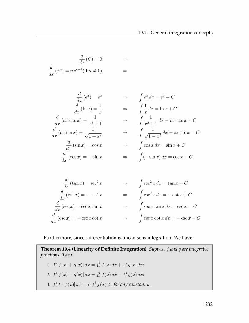
10.1. General integration concepts
d
dx(C) = 0 ⇒
d
dx(xn) = nxn−1(if n 6= 0) ⇒
d
dx(ex) = ex ⇒
∫ex dx = ex + C
d
dx(ln x) = 1
x⇒
∫ 1xdx = ln x+ C
d
dx(arctan x) = 1
x2 + 1 ⇒∫ 1x2 + 1 dx = arctan x+ C
d
dx(arcsin x) = 1√
1− x2⇒
∫ 1√1− x2
dx = arcsin x+ C
d
dx(sin x) = cos x ⇒
∫cosx dx = sin x+ C
d
dx(cosx) = − sin x ⇒
∫(− sin x) dx = cosx+ C
d
dx(tan x) = sec2 x ⇒
∫sec2 x dx = tan x+ C
d
dx(cotx) = − csc2 x ⇒
∫csc2 x dx = − cotx+ C
d
dx(secx) = secx tan x ⇒
∫secx tan x dx = secx = C
d
dx(cscx) = − cscx cotx ⇒
∫cscx cotx dx = − cscx+ C
Furthermore, since differentiation is linear, so is integration. We have:
Theorem 10.4 (Linearity of Definite Integration) Suppose f and g are integrablefunctions. Then:
1.∫ ba [f(x) + g(x)] dx =
∫ ba f(x) dx+
∫ ba g(x) dx;
2.∫ ba [f(x)− g(x)] dx =
∫ ba f(x) dx−
∫ ba g(x) dx;
3.∫ ba [k · f(x)] dx = k
∫ ba f(x) dx for any constant k.
232

10.1. General integration concepts
Theorem 10.5 (Linearity of Indefinite Integration) Suppose f and g are integrablefunctions. Then:
1.∫
[f(x) + g(x)] dx =∫f(x) dx+
∫g(x) dx;
2.∫
[f(x)− g(x)] dx =∫f(x) dx−
∫g(x) dx;
3.∫
[k · f(x)] dx = k∫f(x) dx for any constant k.
NOTE: Integration is not multiplicative nor divisive:∫f(x)g(x) dx 6=
(∫f(x) dx
)·(∫
g(x) dx)
∫ (f(x)g(x)
)dx 6=
∫f(x) dx∫g(x) dx
Example 1: Compute the integral∫−1
4 csc2 x dx
Example 2: Suppose a bicyclist is driving down a road so that her velocity attime t is 3− 2t+ t9.
(a) Find the displacement of the bicyclist from time 1 to time 2.
(b) If the position of the bicyclist at time 0 is 4, find the position at time 1.
Example 3: Compute the integral
∫ (2
3√x
+ 5x
)dx
233

10.1. General integration concepts
Example 4: Compute the integral∫(4 cosx− 3x5 + 2ex) dx
Example 5: Compute the integral∫ (sin x7 + 4
1 + x2 − 2)dx
Here is a list of integration rules which, together with linearity, allows you todo most easy integrals:
Theorem 10.6 (Integration Rules to Memorize) The following integration formu-las hold:
Constant Rules:∫
0 dx = C∫M dx = Mx+ C
Power Rules:∫xn dx = xn+1
n+1 + C (so long as n 6= −1)∫ 1xdx = ln |x|+ C
Trig Functions:∫
sin x dx = − cosx+ C∫cosx dx = sin x+ C∫sec2 x dx = tan x+ C∫csc2 x dx = − cotx+ C∫secx tan x dx = secx+ C∫cscx cotx dx = − cscx+ C
Exponential Functions:∫ex dx = ex + C
Inverse Trig Functions:∫ 1x2+1 dx = arctan x+ C∫ 1√
1−x2 dx = arcsin x+ C
234
10.2. Rewriting the integrand
Note: There are some integrals which we don’t know yet. They include:∫tan x dx
∫cotx dx
∫secx dx
∫sin(x2) dx
∫ln x dx, etc.
Most of these integrals will be discussed in Math 230 (alternatively, some ofthem can be computed using Mathematica, but some integrals are known to beimpossible to compute, even with an infinitely powerful computer!).
10.2 Rewriting the integrandSometimes it is useful to use algebra, or a trigonometric identity, or a logarithm
rule, to rewrite the integrand before computing an integral.
Example: Find the area under the graph of f(x) = (x2−1)2
xbetween x = 1 and
x = 2.
235

10.3. Elementary u-substitutions
Example: Compute the integral ∫tan2 x dx
Example: Compute the integral∫ln (2x) dx
10.3 Elementary u-substitutionsExample: Let f(x) = sin(x3).
Goal: Recognize integrands which arise as the result of the Chain Rule.
Idea: Identify the presence of a function and its derivative in the integrand.
236
10.3. Elementary u-substitutions
Example: (Generalization of preceding example) Consider the functionF (g(x)),where F ′ = f . Then
d
dx[F (g(x))] = F ′(g(x)) · g′(x) = f(g(x)) · g′(x)
Theorem 10.7 (Integration by u−substitution - Indefinite Integrals)∫f(g(x)) · g′(x) dx =
∫f(u) du by setting u = g(x).
Procedure for indefinite integration by u−substitution:
1. Make sure you can’t just “write the answer” to the integral without asubstitution.
2. Check the integrand to make sure a u−substitution is appropriate:• The integral should not be one you have memorized.• The integrand should have two terms multiplied together.• One of the terms being multiplied should be the derivative of part
of the other term (i.e. the terms should be related).
3. Let u = the term whose derivative stands by itself.
4. Write the derivative of u in Leibniz notation, then multiply through byan appropriate constant to match what is in the integral.
5. Substitute in the integral so that all xs are replaced with us asappropriate.
6. Integrate with respect to u.
7. Back-substitute to get an answer in terms of x.
237
10.3. Elementary u-substitutions
A picture to explain the logic:
Example: Compute the integral:∫5(6x2 + 3
)4· 12x dx
238
10.3. Elementary u-substitutions
Example: Compute the integral:∫27(z3 + 1)9z2 dz
Example: Compute the integral:∫tan3(3x+ 1) sec2(3x+ 1) dx
Solution:
Let u = tan(3x+ 1).
⇒ du
dx= sec2(3x+ 1) · 3
⇒ du = 3 sec2(3x+ 1) dx
⇒ 13du = sec2(3x+ 1) dx
239

10.3. Elementary u-substitutions
Example: Compute the integral:∫sin(3x+ 2) dx
Example: Compute the integral:∫(5x− 2)12 dx
Solution:
Let u = 5x− 2
⇒ du
dx= 5
⇒ du = 5 dx
⇒ 15du = dx
Now the integral becomes
∫u12 1
5 du = 15 ·
u13
13 + C = 165u
13 + C = 165(5x− 2)13 + C.
The general principle illustrated by the preceding examples is called the LinearReplacement Principle:
Theorem 10.8 (Linear Replacement Principle) Suppose∫f(x) dx = F (x) + C.
Then for any constants m and b,∫f(mx+ b) dx = 1
mF (mx+ b) + C.
240

10.3. Elementary u-substitutions
Example: Compute the integrals:∫2e5x dx
∫ 42x− 3 dx
Some integrals require rewriting before performing a substitution:
Example: Compute the integral: ∫tan x dx
Example: Compute the integral:∫xe−x
2dx
241

10.3. Elementary u-substitutions
Substitution in definite integrals
Example: Compute the integral:∫ 4
1
1√x(√x+ 1)3 dx
Theorem 10.9 (Integration by u−substitution - Definite Integrals) By way ofthe u-substitution u = g(x),
∫ b
af(g(x)) · g′(x) dx =
∫ g(b)
g(a)f(u) du.
242

10.3. Elementary u-substitutions
Procedure for definite integration by u−substitution:
1. Make sure you can’t just “write the answer” to the integral without asubstitution.
2. Check the integrand to make sure a u−substitution is appropriate:• The integral should not be one you have memorized.• The integrand should have two terms multiplied together.• One of the terms being multiplied should be the derivative of part
of the other term (i.e. the terms should be related).
3. Let u = the term whose derivative stands by itself.
4. Write the derivative of u in Leibniz notation, then multiply through byan appropriate constant to match what is in the integral.
5. Substitute in the integral so that all xs are replaced with us asappropriate.
6. Change the limits of integration to values of u using the formulafrom Step 3.
7. Integrate with respect to u (don’t back-substitute for x).
Example: Find the distance travelled by an object between times 0 and π/2, ifits velocity at time t is ecos t sin t.
243

10.3. Elementary u-substitutions
Example: Compute the integral:
∫ ln 3
0
ex
ex + 1 dx
244

10.4. Homework exercises
10.4 Homework exercisesIn Problems 1-20, compute the indicated integral:
1.∫
0 dx
2.∫ 6
4 5 dx
3.∫ 5
3 x dx
4.∫
4x dx
5.∫
(x+ 3) dx
6.∫ 1
03√x2 dx
7.∫ 4
0 5ex dx
8.∫ 9
24xdx
9.∫
(2x3 − x) dx
10.∫
(sec2 x− 7 sin x) dx
11.∫
( 3x2 + csc2 x) dx
12.∫ π/3π/4 2 secx tan x dx
13.∫ 2
1
(4x2 − 1
)dx
14.∫ ex
4 dx
15.∫ ( 6√
x+ 1
x
)dx
16.∫
(x3/2 + 4x+ 2) dx
17.∫ 1−1(x3 − x2) dx
18.∫dx
19.∫
(2− cscx cotx) dx
20.∫
(x3 + 4 cosx) dx
21. Suppose an object is moving back and forth along a line so that its accelera-tion at time t is a(t) = −5t. If the object’s velocity at time 2 is 3, what is itsvelocity at time 5?
22. Suppose a bee is moving along a number line so that its velocity at time t isv(t) = t2 + 3. If at time 1 the bee is at position −4, what is its position at time4?
23. Suppose a bug is crawling along a number line so that its acceleration at timet is a(t) = 1
10 cos t.
a) If its velocity at time 0 is 15 and its position at time 0 is 1, what is its
position at time π?
b) If its velocity at time 0 is 1 and its position at time 0 is 0, what is itsposition at time π
3 ?
24. Suppose f is a function such that the slope of the line tangent to f at x is4x− 1. If f passes through the point (4, 0), what is f(−2)?
245
10.4. Homework exercises
In Problems 25-30, use Mathematica to compute the indicated integrals (writethe answers as you would write them by hand). Note: Mathematica computes inte-grals using the Integrate command. For example, to compute the definite integral∫ 4
2 x2 dx using Mathematica, execute
Integrate[x^2, {x, 2, 4}]
and to compute the indefinite integral∫x2 dx using Mathematica, execute
Integrate[x^2, x]
(The x in the command is necessary and corresponds to the dx in the integral.)You can also get an integral sign on the Basic Math Assistant.
25.∫
secx dx Note: When you compute an indefinite integral using Mathematica,something is missing from the answer.
26.∫
ln x dx
27.∫ π/4
0 tan x dx
28.∫ 1
0 arctan x dx
29.∫x3e−x dx
30.∫ 3x2−x dx
In Problems 31-52, compute the indicated integral:
31.∫ 8
1
√2xdx
32.∫
(2− x)√x dx
33.∫ x2+2−3x3+1
x4 dx
34.∫ 2
0 (x+ 1)(3x− 2) dx
35.∫ 5−ex
e2x dx
36.∫ (lnx)2
xdx
37.∫ √
3− x2(−2x) dx
38.∫x3(x4 − 1)5 dx
39.∫ 3
2+7x dx
40.∫
5x 3√
1− x2 dx
41.∫ 6x2
1+x3 dx
42.∫ 6x2
(1+x3)3 dx
43.∫
sin πx dx
44.∫
cos 2x dx
45.∫ 1
0 xe−x2
dx
46.∫ 3
4 cos x2 dx
47.∫
tan4 x sec2 x dx
48.∫
cotx dx
246

10.4. Homework exercises
49.∫
3e2x dx
50.∫ 1
0 x(x2 + 1)3 dx
51.∫ 2
1 4x2√x3 + 1 dx
52.∫ 9
11√
x(1+√x)2 dx
Answers
1. C
2. 10
3. 8
4. 2x2 + C
5. 12x
2 + 3x+ C
6. 35
7. 5e4 − 5
8. 4 ln 9− 4 ln 2
9. 12x
4 − 12x
2 + C
10. tan x+ 7 cosx+ C
11. − 3x− cotx+ C
12. 4− 2√
2
13. 1
14. ex
4 + C
15. 12√x+ ln |x|+ C
16. 25x
5/2 + 2x2 + 2x+ C
17. −23
18. x+ C
19. 2x+ cscx+ C
20. 14x
4 + 4 sin x+ C
21. −992
22. 26
23. a) π+65
b) 120 + π
3
24. −18
25. − ln[cos(x/2) − sin(x/2)] +ln[cos(x/2) + sin(x/2)] + C
26. −x+ x ln x+ C
27. ln 22
28. 14(π − ln 4)
29. e−x(−6− 6x− 3x2 − x3) + C
30. 3(ln(1− x)− ln x) + C
31. 8−√
8
32. 43x
3/2 − 25x
5/2 + C
33. −x−3 − x−1 − 3 ln x+ C
34. 6
35. −52 e−2x + e−x + C
36. 13(ln x)3 + C
37. 23(3− x2)3/2 + C
38. 124(x4 − 1)6 + C
39. 37 ln(2 + 7x) + C
40. −158 (1− x2)4/3 + C
41. 2 ln(x3 + 1) + C
42. −(1 + x3)−2 + C
43. −1π
cos πx+ C
44. 12 sin 2x+ C
247

10.4. Homework exercises
45. e−12e
46. 32 sin x
2 + C
47. 15 tan5 x+ C
48. ln(sin x) + C
49. 32e
2x + C
50. 158
51. 24− 169
√2
52. 12
248

Chapter 11
Introduction to DifferentialEquations
11.1 Terminology and examplesMathematics in a nutshell
1. Start with some real-world problem.
2. Build a mathematical model or mathematical object that represents the prob-lem (this often involves writing down variables and equations).
3. Find the solution of the model from Step 2.
4. Generalize the solution and develop the corresponding theory (so you canadapt the solution technique to as many other similar problems as possible).
249
11.1. Terminology and examples
Some examples:
Example 1A rectangle is 3 unitslonger than it is wide.If its area is 54, what
is its side length?
→
Let x = width.x + 3 = length.
A = 54x(x + 3) = 54.
→x = 6
(6× 9)(throw out x = −9)
Example 2 (physics)An object falls toearth, starting at
height 100m. Whatis its height after
t seconds?
Example 3 (biology)If you eat a raw
hamburger, how muchE. coli is in your
system t minutes later?
Example 4(pharmacokinetics)
Give a patient dose Dof a drug every 24 hours.What is the concentration
of the drug in thepatient’s bloodstream
after t hours?
250

11.1. Terminology and examples
The model of Example 1 above is a “numerical equation”:
• both sides of the equation are numbers;
• the object is to solve for numbers x such that the equation holds.
The models of Examples 2, 3 and 4 above are examples of (ordinary) differentialequations (ODEs):
• both sides of the equation are thought of as functions of an independentvariable (t in these examples);
• there is another variable (y in Example 2, x in Example 3, C in Example 4)which depends on that independent variable;
• the equation contains derivatives of the dependent variable with respect tothe independent variable;
• the object is to solve for the explicit relationship between the variables.
More examples of ODEs:
Example 5: y′ + xy = 3x2
Assumption:
This equation can also be written as:
Example 6: x2y′′′ + (x2 − 3xy)y′′ + 2y′y = 3xy′ − 4
Example 7: y′ · y′′′ = y
Assumption:
Example 8: x′′ + c1x′ + c0x = 0 (describes motion of damped oscillator)
Assumption:
251

11.1. Terminology and examples
Example 9: dydt
= 3y
Assumption: y = y(t)
In Example 9,
• y = e3t is a solution because
• y = 2e3t is a solution because
• y = Ke3t is a solution for any constant K because
• y = t2 is not a solution because
Question: Are there any solutions to Example 9 other than y = Ke3t?
252

11.1. Terminology and examples
Some ODEs are particularly easy to solve. Suppose dydx
= g(x) (i.e. there’s onlyan x on the right-hand side). Then
y(x) =∫g(x) dx
by the Fundamental Theorem of Calculus (in particular, notice that there will beinfinitely many solutions, parameterized by a single constant C).
Example 10:dy
dt= 6t2
Example 11: y′′ = 2
These constants (the K in Example 9, the C in Example 10, and the C and Din Example 11) are typical of solutions to ODEs, because solving an ODE is akinto indefinite integration. For a general ODE (not just one of the form dy
dx= g(x),
we expect arbitrary constants in the description of the solution. The number ofconstants in the solution is equal to the highest order of derivative occuring inthe equation, i.e.
y′′′ − 3y = x2 + 3⇒
y + xd2y
dx2 = x3 − dy
dx⇒
y(8) + 3 = x⇒
253

11.2. Vector fields and qualitative analysis of first-order ODEs
Sometimes you know additional information which allows you to solve for theconstant(s):
Example 12: Suppose a bug travels along a line with velocity at time t given byv(t) = 2t− 4. If at time 0, the bug is at position 7, what is the bug’s position at timet?
11.2 Vector fields and qualitative analysis of first-order ODEsDefinition 11.1 An ODE is called first-order if it can be rewritten y′ = g(x, y) forsome function g of x and y.
Example: 3xy′ + 2xy = cos y · y′ − ex
254

11.2. Vector fields and qualitative analysis of first-order ODEs
Suppose we have a first-order ODE y′ = g(x, y). Associated to this ODE is avector field (a.k.a. slope field) in the following sense: at every point (x, y) in theplane, draw a short line segment or arrow of slope g(x, y) passing through (x, y).The collection of all these line segments/arrows is the “vector field” of the ODE.
Example: y′ = 2x
-3 -
5
2-2
-
3
2-1
-
1
2
1
21 3
22 5
23
-3
-2
-1
1
2
3
The vector field suggests what the solutions of the first-order ODE y′ = g(x, y)look like. If y(x) is a solution, then the graph of y(x) must be tangent to all of theline segments associated to all the (x, y) on the graph. Put another way,
“the solutions have to have graphs which flow with the line segments of the vector field”
In the example y′ = 2x, it appears that the solutions are parabolas. That is thecase, because
255
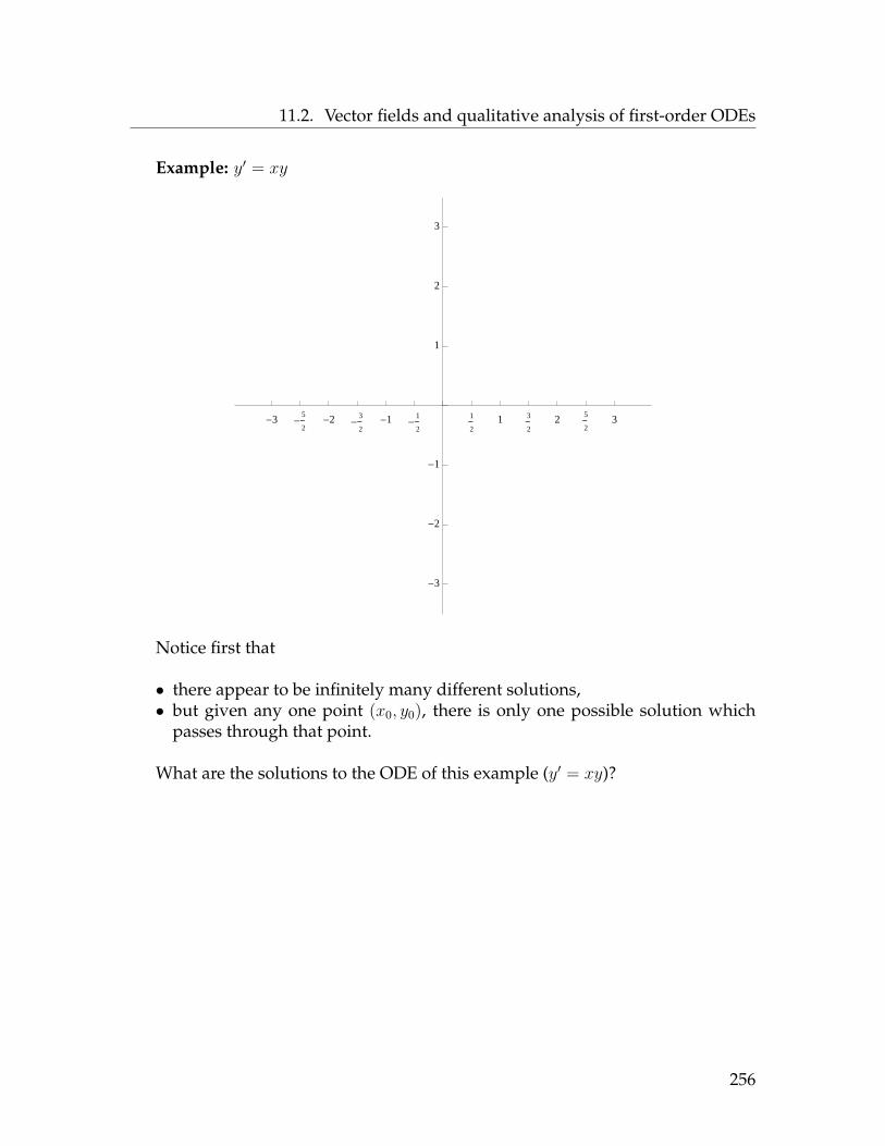
11.2. Vector fields and qualitative analysis of first-order ODEs
Example: y′ = xy
-3 -
5
2-2
-
3
2-1
-
1
2
1
21 3
22 5
23
-3
-2
-1
1
2
3
Notice first that
• there appear to be infinitely many different solutions,• but given any one point (x0, y0), there is only one possible solution which
passes through that point.
What are the solutions to the ODE of this example (y′ = xy)?
256

11.2. Vector fields and qualitative analysis of first-order ODEs
Mathematica is an extremely useful tool for drawing vector fields associated toODEs. To sketch the vector field associated to ODE y′ = g(x, y), use the followingcode (which is explained below). The code is to be typed in one Mathematica celland executed all together.
g[x_,y_] := 3y;VectorPlot[{1,g[x,y]}, {x, -3, 3}, {y, -3, 3},VectorPoints -> 20, Axes -> True,VectorScale -> {Automatic, Automatic, None},VectorStyle -> Orange]
An explanation of the code (and things you can change):
1. The first line defines g(x, y). For example, this code will produce the vectorfield for y′ = 3y.
2. The second line controls the range of the picture; for example, this will sketchthe vector field for x ranging from −3 to 3 and y ranging from −3 to 3.
3. The third line tells Mathematica how many arrows to draw in each direction,and to include the x− and y−axes in the picture.
4. The fourth line controls the size of the arrows and is optional, but I thinkthese choices make for a nice picture.
5. The last line tells Mathematica what color to draw the arrows.
Note: In principle, you don’t type this code over and over. You can get thiscode from the file “vectorfields.nb” (available on my webpage) and you simplycopy and paste the cells into your Mathematica notebooks, editing the formula forg(x, y) and the plot range as necessary.
The above code produces this picture:
-3 -2 -1 0 1 2 3
-3
-2
-1
0
1
2
3
257

11.2. Vector fields and qualitative analysis of first-order ODEs
As mentioned earlier, solutions to an ODE must “flow with” the vector field ofthe ODE. This allows you to qualitatively study solutions to ODEs by examiningthe picture of the vector field associated to the ODE.
Example: Below is a picture of the vector field associated to some first-orderODE y′ = g(x, y):
-6 -4 -2 0 2 4 6
-6
-4
-2
0
2
4
6
1. Write the equation of two explicit solutions to this ODE:
2. On the above picture, sketch the graph of the solution satisfying y(−2) = 1.
3. Suppose y(−2) = 0. Estimate y(2).
4. Suppose y(0) = 3. Find limx→∞
y(x).
5. Suppose y(2) = 0. Find limx→−∞
y(x).
258

11.3. Solving separable ODEs
In many of the questions of the previous example, you are given a point (x0, y0)that the solution of the ODE is to pass through (for example, in Question 2 you aregiven x0 = −2, y0 = 1).
Definition 11.2 A point (x0, y0) through which a solution to an ODE must pass iscalled an initial value. An ODE, together with an initial value, is called an initialvalue problem. A solution of an initial value problem is called a particular solu-tion of the ODE; the set of all particular solutions of the ODE is called the generalsolution of the ODE.
Example: y′ = 2x is a first-order ODE, whose general solution is y = x2 + C.{y′ = 2xy(0) = 1 is an initial value problem, whose particular solution is y = x2 + 1.
Our observation that solutions to ODEs have to “flow with” the vector fieldleads to the following important theorem:
Theorem 11.3 (Existence / Uniqueness Theorem for First-Order ODEs) Givena “reasonable” first-order ODE and an initial value (x0, y0), there is one and only onesolution of that ODE satisfying that initial value.
Logic behind this theorem:
11.3 Solving separable ODEsIn the previous section we learned how to study a first-order ODE qualitatively
(by looking at a picture of the associated vector field).
259

11.3. Solving separable ODEs
Question: Can you explicitly solve a first-order ODE y′ = g(x, y) for the solu-tions y(x)?
Answer:
Definition 11.4 A first-order ODE is called separable if it can be rewritten in theform f(y)y′ = h(x) for functions f of y and h of x.
In other words, an ODE is separable if one can separate the variables, i.e. putall the y on one side and all the x on the other side.
Theoretical solution of separable, first-order ODEs
Suppose you have a separable, first-order ODE. Then, by replacing the y′ with dydx
,it can be rewritten as
f(y) dydx
= h(x).
Integrate both sides with respect to x to get
∫f(y) dy
dxdx =
∫h(x) dx
On the left-hand side, perform the u−substitution u = y(x), du = dydxdx to get∫
f(u) du =∫h(x) dx
Assuming F and H are antiderivatives of f and h, respectively, we get
F (u) = H(x) + C
which, since u = y = y(x), is equivalent to the solution
F (y) = H(x) + C.
Note: We only need a constant on one side of the equation, because the constantson the two sides can be combined into one.
260

11.3. Solving separable ODEs
A shortcut:
The following method involves the writing of things that are technically incorrect,but always works. Again start with a separable, first-order ODE. Again, replacethe y′ with dy
dxto get
f(y) dydx
= h(x).
Now, pretend that the dydx
is a fraction and “multiply” through by dx to get
f(y) dy = h(x) dx.
Now, integrate both sides: ∫f(y) dy =
∫h(x) dx
This gives the same solution as before:
F (y) = H(x) + C.
The shortcut above suggests the following method to solve separable ODEs:
Procedure to solve separable ODEs:
1. Replace y′ with dydx
in the equation.
2. Separate the variables, i.e. put all the y (with the dy) on one side of theequation, and all the x (with the dx) on the other side of the equation.
3. Integrate both sides, putting the arbitrary constant on one side.
4. If the problem contains an initial value, plug it in for x and y and solve forthe constant.
5. If the problem asks for a solution of the form y(x), solve the solution for y.
261

11.3. Solving separable ODEs
Example: y′ = xy(Recall that this example was studied qualitatively on page 256.)
Example: Solve the following initial value problem:{y′ = 2x− 2xyy(1) = −2
262

11.4. Exponential and logistic models
Example: Solve the ODE y′ = −xy
. Without sketching a vector field, describegeometrically what the graphs of the solutions look like.
11.4 Exponential and logistic modelsExample: Experiments have shown that the rate at which a radioactive element
decays is directly proportional to the amount present. (Radioactive elements arechemically unstable elements that decay, or decompose, into stable elements astime passes.) Suppose that if you start with 20 grams of a radioactive substance, in2 years you will have 15 grams of radioactive substance left.
1. How much radioactive substance will you have after 7 years?
2. How long will it take for you to only have 5 grams of radioactive substanceleft?
263

11.4. Exponential and logistic models
Exponential growth and decay
The preceding example can be generalized as follows:
Whenever the rate of change of quantity y is proportional to y itself, then y(t)satisfies the ODE
y′ = ky,
where k is called the proportionality constant. This ODE has solution
y(t) = Cekt
where C = y(0) is the initial amount of quantity y present in the system.
When k < 0, this model is called exponential decay. We see the following:
When k > 0, this model is called exponential growth. We see the following:
Example: The amount of money in an account increases via an exponentialgrowth model. If there is $200 in the account initally and $350 in the account after3 years, how much will be in the account after 10 years?
264

11.4. Exponential and logistic models
Logistic growth and decay
Population biology models seek to determine or estimate the population y of aspecies in terms of the time t. Suppose the species reproduces at rate K. Thismeans that the rate of change in y should be something like K times y. This makessense if the population is small. But if the population gets too big (say greater thansome number L), there is not enough food in the ecosystem to support all of theorganisms, so the population won’t grow despite reproduction, because the organ-isms starve. A differential equation representing this type of situation is called alogistic equation and has the following form:
y′ = K y (L− y)
In a logistic equation, K is a constant called the rate of reproduction and L is aconstant called the carrying capacity or limiting capacity of the system.
In the lab assignment on differential equations, you are asked to sketch picturesof vector fields associated to logistic equations with various K and L.
Question: What is the general solution of a logistic equation?
Solution: First, a preliminary algebra calculation (related to something youlearn in Math 230 called “partial fraction decompositions”):[ 1
L
y+
1L
L− y
]=
1L
(L− y)y(L− y) +
1L
(y)y(L− y) =
1L
(L− y + y)y(L− y) =
1L
(L)y(L− y) = 1
y(L− y) .
Now for the differential equation:
dy
dx= K y (L− y)
1y(L− y) dy = K dx[ 1
L
y+
1L
L− y
]dy = K dx (by the algebra calculation above)
∫ [ 1L
y+
1L
L− y
]dy =
∫K dx
1L
ln y − 1L
ln(L− y) = Kx+ C
ln y − ln(L− y) = KLx+ C
265
11.4. Exponential and logistic models
Because the method of solution on the previous page is so long and compli-cated, the answer we get should be memorized:
Theorem 11.5 (Solution of the logistic equation) The general solution of the lo-gistic equation y′ = Ky(L− y) is
y = L
1 + Ce−KLt.
Example: Suppose you release 1000 elk into a game refuge. Suppose that 5years later there are 104 elk. If the carrying capacity of the game refuge is 4000 elk,and the elk population follows a logistic model, how many elk will be in the gamerefuge 15 years after the initial release?
266
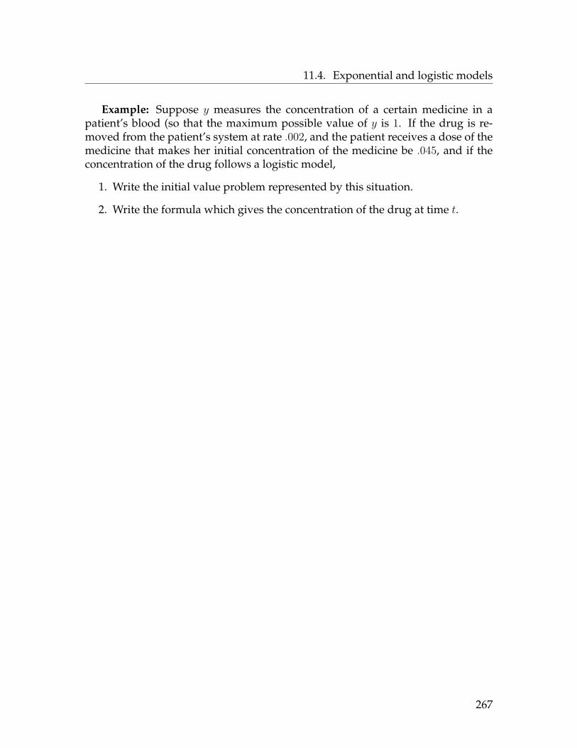
11.4. Exponential and logistic models
Example: Suppose y measures the concentration of a certain medicine in apatient’s blood (so that the maximum possible value of y is 1. If the drug is re-moved from the patient’s system at rate .002, and the patient receives a dose of themedicine that makes her initial concentration of the medicine be .045, and if theconcentration of the drug follows a logistic model,
1. Write the initial value problem represented by this situation.
2. Write the formula which gives the concentration of the drug at time t.
267

11.5. Homework exercises
11.5 Homework exercises1. Verify that the equation y = 3e4x is a solution of the differential equationy′ = 4y.
2. Verify that for any constant C, y = Ce4x is a solution of the differential equa-tion y′ = 4y.
3. Verify that for any constant C, y = Cex2 is a solution of the differential equa-
tion dydx
= 2xy.
4. Verify that the equation y = sin x cosx− cos2 x is a solution of the differentialequation 2y + y′ = 2 sin(2x)− 1 satisfying y(π/4) = 0.
5. Solve for y if dydx
= 3x2.
6. Solve for y if dydx
= x−2x
.
7. Solve for y if d2ydx2 = x−2.
In Problems 8-11, use Mathematica to sketch the vector field corresponding tothe given first-order ODE (the appropriate Mathematica code can be found on page257 or in the file vectorfields.nb on Blackboard). Your viewing window shouldbe [−6, 6]× [−6, 6].
8. dydx
= 110y(4− y)
9. dydx
= xx+y
10. dydx
= 2xy − y2
11. dydx
= e−x sin(πy)
12. Consider the first-order ODE dydx
= 15x cos(πy/6).
a) Use Mathematica to sketch the vector field associated to this ODE.
b) Based on the picture you see, give one explicit solution of the ODE.
c) Let y = f(x) be the solution to this ODE passing through the origin.Find lim
x→∞f(x) and lim
x→−∞f(x).
d) Let y = f(x) be as in part (c). Estimate f(4) and f(−4).
e) Let y = h(x) be the solution to this ODE passing through (0,−2). Esti-mate the smallest positive value of x such that h(x) = 0.
268

11.5. Homework exercises
13. Consider the first-order ODE dydx
= 14(y3 − 16y).
a) Use Mathematica to sketch the vector field associated to this ODE.
b) Based on the picture you see, give three explicit solutions of the ODE.
c) Let y = f(x) be the solution to this ODE passing through (0, 1). Findlimx→∞
f(x).
d) Let y = h(x) be the solution to this ODE passing through (2,−2). Findlimx→∞
h(x).
14. Consider the first-order ODE dydx
= 2x+ y.
a) Use Mathematica to sketch the vector field associated to this ODE.
b) Let y = f(x) be the solution to this ODE passing through (−1, 1). Esti-mate f(1).
In Problems 15-17, solve the indicated differential equation.
15. dydx
= xy
16. (2 + x)y′ = 3y
17. yy′ = sin x
In Problems 18-22, solve the indicated initial value problem.
18.{ √
x+√yy′ = 0y(1) = 4
19.{y(1 + x2)y′ − x(1 + y2) = 0y(0) =
√3
20.{yy′ − ex = 0y(0) = 6
21.{
dydx
= ex−2y
y(0) = 0
22.{
dydx
= y4+x
y(0) = 1
23. Suppose you have 300 mg of a radioactive substance initially, and that after8 years you have 280 mg of the substance remaining.
a) How much will you have left after 35 years?
b) How long will it take you to have 200 mg of the substance left?
24. Radioactive radium has a half-life of 1599 years (this means that if you startwith a certain amount of it, after 1599 years you will have half as much asyou started with). What percent of an initial sample of radium will be presentafter 100 years?
269
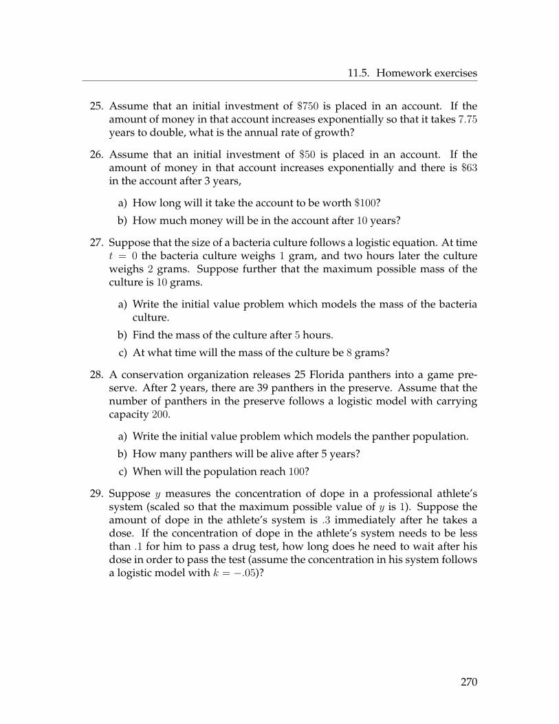
11.5. Homework exercises
25. Assume that an initial investment of $750 is placed in an account. If theamount of money in that account increases exponentially so that it takes 7.75years to double, what is the annual rate of growth?
26. Assume that an initial investment of $50 is placed in an account. If theamount of money in that account increases exponentially and there is $63in the account after 3 years,
a) How long will it take the account to be worth $100?
b) How much money will be in the account after 10 years?
27. Suppose that the size of a bacteria culture follows a logistic equation. At timet = 0 the bacteria culture weighs 1 gram, and two hours later the cultureweighs 2 grams. Suppose further that the maximum possible mass of theculture is 10 grams.
a) Write the initial value problem which models the mass of the bacteriaculture.
b) Find the mass of the culture after 5 hours.
c) At what time will the mass of the culture be 8 grams?
28. A conservation organization releases 25 Florida panthers into a game pre-serve. After 2 years, there are 39 panthers in the preserve. Assume that thenumber of panthers in the preserve follows a logistic model with carryingcapacity 200.
a) Write the initial value problem which models the panther population.
b) How many panthers will be alive after 5 years?
c) When will the population reach 100?
29. Suppose y measures the concentration of dope in a professional athlete’ssystem (scaled so that the maximum possible value of y is 1). Suppose theamount of dope in the athlete’s system is .3 immediately after he takes adose. If the concentration of dope in the athlete’s system needs to be lessthan .1 for him to pass a drug test, how long does he need to wait after hisdose in order to pass the test (assume the concentration in his system followsa logistic model with k = −.05)?
270

11.5. Homework exercises
Answers
1. y′ = 12e4x = 4y.
2. y′ = 4Ce4x = 4y.
3. y′ = Cex22x = 2xy.
4. Differentiate to get y′ = cos2 x −sin2 x + 2 sin x cosx. Now 2y +y′ = 2 sin x cosx−2 cos2 x+cos2 x−sin2 x+ 2 sin x cosx = 4 sin x cosx−1 = 2 sin 2x − 1 as desired. Last,y(π/4) = 0 by direct calculation.
5. y = x3 + C
6. y = x− 2 ln x+ C
7. y = − ln x+ Cx+D
8. -6 -4 -2 0 2 4 6
-6
-4
-2
0
2
4
6
9. -6 -4 -2 0 2 4 6
-6
-4
-2
0
2
4
6
10. -6 -4 -2 0 2 4 6
-6
-4
-2
0
2
4
6
11. -6 -4 -2 0 2 4 6
-6
-4
-2
0
2
4
6
12. a) -6 -4 -2 0 2 4 6
-6
-4
-2
0
2
4
6
b) y = 3 (also y = −3, y = 9, y =−9)
c) Both answers are 3.
d) Both answers are about 1.7.
e) Roughly x = 5.
271

11.5. Homework exercises
13. a) -6 -4 -2 0 2 4 6
-6
-4
-2
0
2
4
6
b) y = 4, y = 0, y = −4c) 0d) 0
14. a) -6 -4 -2 0 2 4 6
-6
-4
-2
0
2
4
6
b) 1
15. 12y
2 = 12x
2 + C
16. ln y = 3 ln(x+2)+C (this simplifiesto y = K(x+ 2)3
17. 12y
2 = − cosx+ C
18. y = (9− x3/2)2/3
19. 1+y2
1+x2 = 4
20. 12y
2 = ex + 17
21. 12e
2y = ex − 12
22. ln y = ln(x+4)−ln 4 (this simplifiesto y = 1
4(x+ 4)
23. a) 221.836 mg
b) 47 years
24. 95.7%
25. 8.943%
26. a) 8.9976 years
b) $108.03
27. a){y′ =
(120 ln 9
4
)y(10− y)
y(0) = 1b) 270
59
c) t ≈ 8.838
28. a){y′ =
(120 ln 9
4
)y(10− y)
y(0) = 25b) 70c) After 7.37 years
29. 27 days
272

Appendix A
Mathematica reference
A.1 Quick reference guideStandard computations
Expression Mathematica syntaxxy x y (don’t forget the space)e E (or use Basic Math Assistant palette)π Pi (or use Basic Math Assistant palette)∞ Infinity (or use Basic Math Assistant palette)
√32 Sqrt[32] (or use Basic Math Assistant palette)
4√
40 40^(1/4) (or use Basic Math Assistant palette)
|x− 3| Abs[x-3]
sin π Sin[Pi]cos(x(y + 1)) Cos[x(y+1)]cot
(2π3 + 3π
4
)Cot[2 Pi/3 + 3 Pi/4]
arctan 1 ArcTan[1]
ln 3 Log[3]log6 63 Log[6,63]log 18 Log10[18]
27y 2^(7y) (or use Basic Math Assistant palette)ex−5+x2 E^(x-5+x^2) or Exp[x-5+x^2]
(or use Basic Math Assistant palette)
273

A.1. Quick reference guide
Expression Mathematica syntaxf(x+ 3) (if f is a function) f[x+3]
xf(2x)− x2f(x) x f[2x] - x^2 f[x] (don’t forget spaces)(f ◦ g)(x) f[g[x]]
limx→4
f(x) Limit[f[x], x -> 4]f ′(3) f’[3]g′′′(x) g’’’[x] or D[g[x],{x,3}]∫x2 dx Integrate[x^2,x]
(or use Basic Math Assistant palette)∫ 52 cosx dx Integrate[Cos[x], {x, 2, 5}]
(or use Basic Math Assistant palette)(for decimal approximation, use NIntegrate)
12∑k=1
f(k) Sum[f[k], {k, 1, 12}]
30! (factorial) 30!
Objective Mathematica syntaxTo call the preceding output %
To get a decimal approx. N[%] (or click numerical value)to the preceding output
Perform partial fraction Apart[ ]decomposition
Object keyboard shortcutraised exponent type base, then [Control]+6, then exponent
horizontal fraction bar type [Control]+/, then numerator,then [Tab], then denominator
square root sign [Control]+2
274

A.1. Quick reference guide
Basic commands with functions and graphs
Objective Mathematica syntaxDefine a function f[x_] = formulaf(x) = formula (one equals sign, underscore after x)
Generate table of values for f Table[{x,f[x]}, {x,xmin,xmax,step}]
Plot the graph of Plot[formula, {x,xmin,xmax}]f(x) = formula
Plot multiple graphs at once Plot[{formula,formula, ..., formula},{x,xmin,xmax}]
Plot the graph of Plot[formula, {x,xmin,xmax},f(x) = formula with PlotRange -> {ymin,ymax}]range of y−values specified
Plot the graph of Plot[formula, {x,xmin,xmax},f(x) = formula with PlotRange -> {ymin,ymax},range of y−values specified AspectRatio -> Automatic]with x- and y-axeson same scale
Objective Mathematica syntaxDefine parametric function f[t_] = {f(t),g(t)}x = f(t), y = g(t)
Plot graph of a set ParametricPlot[f[t], {t, -20,20},of parametric equations PlotRange -> {{xmin,xmax},(after defining them as f(t)) {ymin,ymax}}]
275

A.2. Code for derivatives
Commands to solve equations
Objective Mathematica syntaxFind exact solution(s) Solve[lhs==rhs,x]to equation (two equals signs)of form lhs = rhs (works only with polynomials or other
relatively “easy” equations)
Find decimal approx. NSolve[lhs==rhs,x]to solutions of (two equals signs)equation lhs = rhs (works only with “easy” equations)
Find decimal approx. FindRoot[lhs==rhs,{x,guess}]to solutions of (two equals signs)equation lhs = rhs
A.2 Code for derivativesSuppose you wanted to find the derivative of f(x) = sin x. There are a variety
of ways to do this:
First method: Define the function as usual, then use the apostrophe to make aprime. For example, executing
f[x_] = Sin[x]
then
f’[x]
will produce the derivative as its output. Similarly,
f’[3]
will give the value of the derivative at x = 3 and
f’’[x]
276
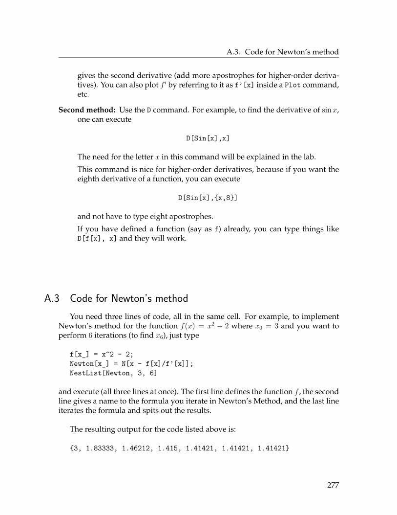
A.3. Code for Newton’s method
gives the second derivative (add more apostrophes for higher-order deriva-tives). You can also plot f ′ by referring to it as f’[x] inside a Plot command,etc.
Second method: Use the D command. For example, to find the derivative of sin x,one can execute
D[Sin[x],x]
The need for the letter x in this command will be explained in the lab.
This command is nice for higher-order derivatives, because if you want theeighth derivative of a function, you can execute
D[Sin[x],{x,8}]
and not have to type eight apostrophes.
If you have defined a function (say as f) already, you can type things likeD[f[x], x] and they will work.
A.3 Code for Newton’s methodYou need three lines of code, all in the same cell. For example, to implement
Newton’s method for the function f(x) = x2 − 2 where x0 = 3 and you want toperform 6 iterations (to find x6), just type
f[x_] = x^2 - 2;Newton[x_] = N[x - f[x]/f’[x]];NestList[Newton, 3, 6]
and execute (all three lines at once). The first line defines the function f , the secondline gives a name to the formula you iterate in Newton’s Method, and the last lineiterates the formula and spits out the results.
The resulting output for the code listed above is:
{3, 1.83333, 1.46212, 1.415, 1.41421, 1.41421, 1.41421}
277

A.4. Code for Riemann sums
These numbers are x0, x1, x2, ..., x6 so for example, x2 = 1.46212 and x4 = 1.41421...and x6 = 1.41421 (the same as x4 to 5 decimal places).
To implement Newton’s method for a different function, different initial guessand different number of iterations, simply change the formula for f , change the 3to the appropriate value of x0 and the 6 to the number of times you want to iterateNewton’s method.
A.4 Code for Riemann sumsIn this section we discuss how to compute left- and right- Riemann sums us-
ing Mathematica. Ultimately, to do a Riemann sum you need to execute three com-mands found later in this section; for now we explain where these commands comefrom.
1. Defining the function f
First, recall that to define a function you use an underscore. For example, thefollowing command defines f to be the function f(x) = x2:
f[x_] = x^2
2. Defining the partition P
Defining a partition in Mathematica is easy. Just use braces, and list the numbersfrom smallest to largest. For example, to define the partition P = {0, 1, 5
2 , 4, 7}, justexecute
P = {0, 1, 5/2, 4, 7}
We often use partitions which divide [a, b] into n equal-length subintervals. Tocreate such a partition in Mathematica, use the Range command. For example, todefine a partition of [0, 2] into 10 equal-length subintervals, execute the following:
P = Range[0, 2, (2-0)/10]
278
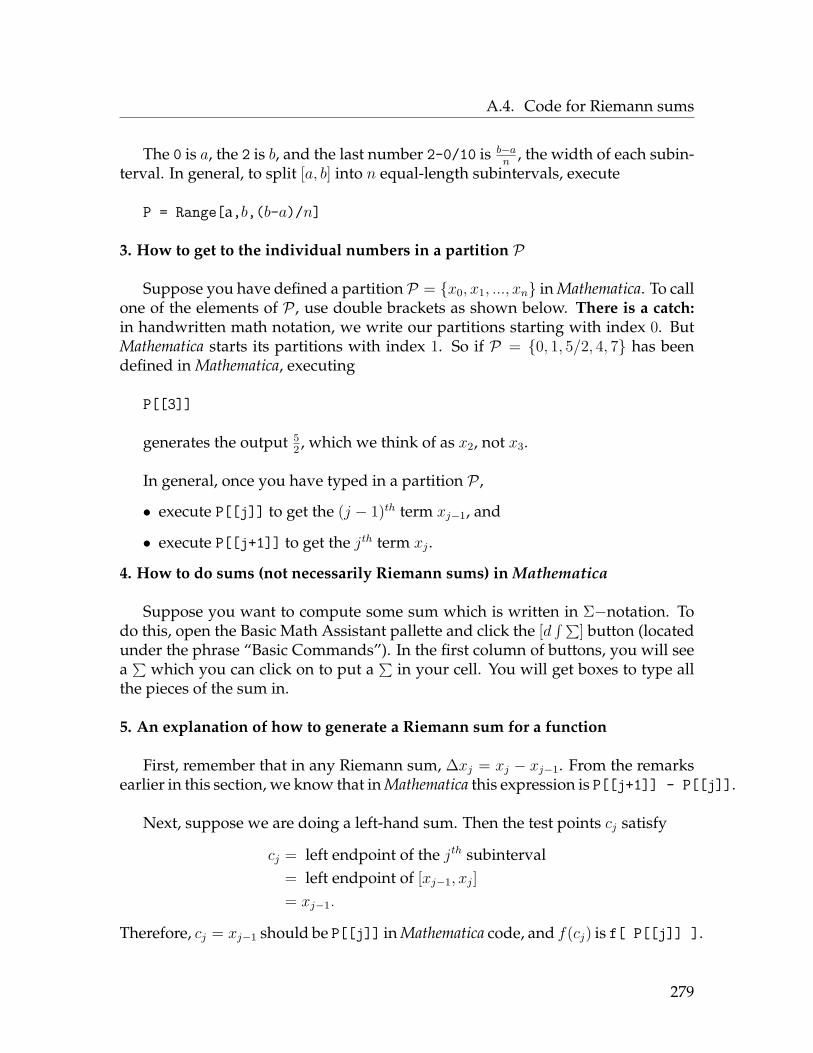
A.4. Code for Riemann sums
The 0 is a, the 2 is b, and the last number 2-0/10 is b−an
, the width of each subin-terval. In general, to split [a, b] into n equal-length subintervals, execute
P = Range[a,b,(b-a)/n]
3. How to get to the individual numbers in a partition P
Suppose you have defined a partitionP = {x0, x1, ..., xn} in Mathematica. To callone of the elements of P , use double brackets as shown below. There is a catch:in handwritten math notation, we write our partitions starting with index 0. ButMathematica starts its partitions with index 1. So if P = {0, 1, 5/2, 4, 7} has beendefined in Mathematica, executing
P[[3]]
generates the output 52 , which we think of as x2, not x3.
In general, once you have typed in a partition P ,
• execute P[[j]] to get the (j − 1)th term xj−1, and
• execute P[[j+1]] to get the jth term xj .
4. How to do sums (not necessarily Riemann sums) in Mathematica
Suppose you want to compute some sum which is written in Σ−notation. Todo this, open the Basic Math Assistant pallette and click the [d
∫ ∑] button (locatedunder the phrase “Basic Commands”). In the first column of buttons, you will seea∑
which you can click on to put a∑
in your cell. You will get boxes to type allthe pieces of the sum in.
5. An explanation of how to generate a Riemann sum for a function
First, remember that in any Riemann sum, ∆xj = xj − xj−1. From the remarksearlier in this section, we know that in Mathematica this expression is P[[j+1]] - P[[j]].
Next, suppose we are doing a left-hand sum. Then the test points cj satisfy
cj = left endpoint of the jth subinterval= left endpoint of [xj−1, xj]= xj−1.
Therefore, cj = xj−1 should be P[[j]] in Mathematica code, and f(cj) is f[ P[[j]] ].
279

A.4. Code for Riemann sums
Putting this together, the right Mathematica code for a left-hand Riemann sum(assuming you have defined your function f and your partition P) is
n∑j = 1
f[ P[[j]] ] (P[[j + 1]] - P[[j]])
6. The final commands for left- and right-hand Riemann sums
From above, we came up with the following sequence of commands for com-puting a left-hand Riemann sum:
Syntax to compute a left-hand Riemann sum
To evaluate a left-hand Riemann sum, execute the following commands:
f[x_] = x^2(or whatever your function is)
P = {0, 1/2, 3/4, 1}(or whatever your partition is)
∑nj = 1 f[ P[[j]] ] (P[[j+1]] - P[[j]])(n is the number of subintervals)
To evaluate a right-hand sum, the only thing that changes is the test point cj ,which goes from the left endpoint xj−1 (i.e. P[[j]]) to the right endpoint xj (i.e.P[[j+1]]). Thus the commands for computing a right-hand Riemann sum aresimilar:
280

A.5. Code for producing pictures of vector fields
Syntax to compute a right-hand Riemann sum
To evaluate a right-hand Riemann sum, execute the following commands:
f[x_] = x^2(or whatever your function is)
P = {0, 1/2, 3/4, 1}(or whatever your partition is)
∑nj = 1 f[ P[[j+1]] ] (P[[j+1]] - P[[j]])(n is the number of subintervals)
A.5 Code for producing pictures of vector fieldsCode to plot a vector field:
Here is an example of the syntax which produces the vector field associated to afirst-order ODE (type this all in one cell):
g[x_,y_] : = 3y;VectorPlot[{1,g[x,y]},{x,-3,-3},{y,-3,3}, VectorPoints -> 20,Axes -> True, VectorScale -> {Automatic, Automatic, None},VectorStyle -> Orange]
What this command does: First, the function g(x, y) is defined in the first line. Ifyou wanted to sketch a vector field for a different equation, you can change the 3yhere to whatever formula is given by g(x, y). Second, the VectorPlot commandtells Mathematica to sketch the vector field. The relevant ingredients here are asfollows:
• The {x, -3, 3} and {y, -3, 3} tell Mathematica to produce a picture thatruns from x = −3 to x = 3 and y = −3 to y = 3, i.e. it specifies the range ofthe picture.
• The VectorPoints -> 20 tells Mathematica how many vectors to draw. Ifyou change 20 to a larger number, you get more densely drawn arrows. This
281

A.5. Code for producing pictures of vector fields
produces a more accurate picture of the vector field, but the program willtake longer to run. On the other hand, if you change 20 to a smaller (positive)number, less arrows will be drawn, resulting in a less dense picture.
• The Axes -> True tells Mathematica to draw the x- and y- axes on the picture.• The VectorScale -> {Automatic, Automatic, None} tells Mathematica to make
sure all the vectors are scaled so that you can see them (without this com-mand many of the vectors drawn would be too small to see).
• The VectorStyle -> Orange tells Mathematica to make the vectors orange.An interesting thing to do is to replace this command with the followingphrase: VectorColorFunction -> Hue to get a ’tie-dye’ looking picture.
Code to produce a stream plot:
Here is a command which plots both the vector field and some solution curves tothe differential equation y′ = g(x, y). It comes from taking the command aboveand adding some additional programming inside the VectorPlot command:
g[x_,y_] : = 3y;VectorPlot[{1,g[x,y]},{x,-3,-3},{y,-3,3}, VectorPoints -> 20,Axes -> True, VectorScale -> {Automatic, Automatic, None},VectorStyle -> Orange, StreamPoints -> 35, StreamScale -> Full,StreamStyle -> {Blue, Thick}]
As before, the first line defines g(x, y); the {x, -3, 3} and {y, -3, 3} deter-mine the range of the picture; the VectorPoints -> 20 tell Mathematica how manyarrows to draw; Axes -> True tells Mathematica to draw the x- and y- axes; andthe VectorScale command ensures the vectors are big enough to see.
What’ s new here are the commands regarding "Streams". The StreamPoints -> 35asks Mathematica to draw 35 stream lines (a stream line is a graph that ’ follows’the vector field as described in lecture). If you lower the number 35, less streamlines are drawn and if you increase the number, more stream lines are drawn.
The StreamScale -> Full command ensures that the stream lines are connectedwhen they should be (so that you get a much better picture). The last bit tells Math-ematica what color to make the stream lines and to make them thick.
Code to produce a steam plot through a particular point:
Suppose you wanted to draw one stream line that went through one specifiedpoint. In this case, you modify the above command by changing the StreamPointsdirective from 35 to {{a,b}} where you want to draw the stream line through the
282

A.5. Code for producing pictures of vector fields
point (a, b). For example, in the above picture, if you wanted the stream line pass-ing through the point (1, 2), your command would be :
g[x_,y_] : = 3y;VectorPlot[{1,g[x,y]},{x,-3,-3},{y,-3,3}, VectorPoints -> 20,Axes -> True, VectorScale -> {Automatic, Automatic, None},VectorStyle -> Orange, StreamPoints -> {{1,2}}, StreamScale -> Full,StreamStyle -> {Blue, Thick}]
283

Index
Σ-notation, 205e, 8nth Derivative Test, 157nth derivative, 104u-substitution, definite integrals, 240u-substitution, indefinite integrals, 235
absolute maximum, 146absolute maximum value, 146absolute minimum, 146absolute minimum value, 146acceleration, 105additivity property of integrals, 213antiderivative, 217Antiderivative Theorem, 217arcsin x, derivative of, 133arcsine, definition of, 25arcsine, graph of, 25arctan x, derivative of, 133arctangent, definition of, 25arctangent, graph of, 25arithmetic with∞, 59asymptote, horizontal, 46asymptote, vertical, 45
carrying capacity, 263Chain Rule, 121, 123Chain Rule vs. Product Rule, 125Chain Rule, Leibniz notation, 121Chain Rule, prime notation, 123
change of base formula (exponents),10
change of base formula (logarithms),10
common logarithm, 8composition (of functions), 15concave down, 155concave up, 155concavity, 155Concavity Test, 156Constant Function Rule, 90Constant Multiple Rule, 95constrained optimization problem, 144constraint, 143continuous, 57continuous at a point, 55continuous functions, evaluating limit
of, 65continuous on an interval, 57CP, 149critical point, 149Critical Point Theorem, 149
decreasing, 154definite integral, 212definite integral, definition of, 212definition of derivative, 81definition of the definite integral, 212derivative, 81derivative of exponential function, 103
284
Index
derivative of logarithmic function, 103derivative of trig functions, 100, 119derivative, definition of, 81derivative, list of rules, 135derivative, units of, 82Difference Rule, 94differential equation, 249differentials, 176differentiate, 81differentiation rules, summary, 135differentiation, implicit, 128, 130discontinuity, infinite, 56discontinuity, jump, 55, 56discontinuity, oscillating, 56discontinuity, removable, 55discontinuous at a point, 55displacement, 202domain (of a function), 12
error (in an approximation), 210error bound, 210Error bound for Riemann sums, 211Euler’s constant, 8Existence-Uniqueness Theorem for first-
order ODEs, 257Exponent rules, 5exponent rules, 7exponential decay, 262exponential function, derivative of, 103exponential growth, 262extrema, 146
first derivative, 104first-order ODE, 252flowchart for evaluating limits, 60free optimization problem, 144function, 12functions, operations on, 15Fundamental Theorem of Calculus Part
I, 218Fundamental Theorem of Calculus Part
II, 219
general solution (of ODE), 257global maximum, 146global minimum, 146graph (of a function), 14graphs of common functions, 17
higher-order derivative, 104hole discontinuity, 55horizontal asymptote, 46
implicit differentiation, 128, 130increasing, 154indefinite integral, 228indeterminate form, 59, 178inequality properties of integrals, 214infinite discontinuity, 56infinite limits, 44infinity, arithmetic rules with, 59inflection point, 155initial value, 257initial value problem, 257instantaneous velocity, 80, 82integrable, 212integral, additivity property of, 213integral, definite, 212integral, definite vs. indefinite, 229integral, indefinite, 228integral, inequality properties of, 214integral, linearity properties of, 213integration by u-substitution (definite
integrals), 240integration by u-substitution (indefi-
nite integrals), 235integration rules, 232Inverse Function Theorem, 134inverse sine, definition of, 25inverse tangent function, definition of,
25inverse trig functions, definition of, 25
jump discontinuity, 56
L’Hôpital’s Rule, 179left Riemann sum, 208
285

Index
left-hand limits, 41Leibniz notation, 82limit at infinity, 45limit at infinity, evaluating, 61limit flowchart, 60limit, approximation via tables, 37limit, formal definition, 40limit, graphical interpretation, 36limit, infinite, 44limit, left-hand, 41limit, one-sided, 41limit, right-hand, 41limiting capacity, 263linear approximation, 172Linear Function Rule, 90Linear Replacement Principle, 238local maximum, 146local maximum value, 146local minimum, 146local minimum value, 146logarithm base b, 8logarithm rules, 9logarithm, common, 8logarithm, definition, 8logarithm, natural, 8logarithmic differentiation, 127logarithmic function, derivative of, 103logistic equation, 263logistic equation, solution of, 264lower Riemann sum, 208
Main Limit Theorem, 58Max-Min Existence Theorem, 148Max-Min Inequality, 214maximum, absolute, 146maximum, global, 146maximum, local, 146maximum, relative, 146Mean Value Theorem, 216minimum, absolute, 146minimum, global, 146minimum, local, 146
minimum, relative, 146monotone, 154Monotonicity Law, 214Montonicity Test, 155
natural logarithm, 8Newton’s method, 184Newton’s method, Mathematica code,
186, 275Newton’s method, problems with, 187norm (of a partition), 206
ODE, 249ODE, first-order, 252one-sided limits, 41operations on functions, 15optimization problem, 148optimization problem, constrained, 144optimization problem, free, 144optimization procedure, 149, 151ordinary differential equation, 249oscillating discontinuity, 56
particular solution (of ODE), 257partition, 206piecewise-defined function, 16piecewise-defined functions, evaluat-
ing limit of, 64point-slope formula, 19Positivity Law, 214Power Rule, 93Product Rule, 114Product Rule vs. Chain Rule, 125properties of arcsine and arctangent,
25proportionality constant, 262
quadratic approximation, 174Quotient Rule, 116
range (of a function), 12rate of reproduction (logistic equation),
263related rates, 190
286

Index
relative maximum, 146relative minimum, 146removable discontinuity, 55Riemann sum, 207Riemann sums, error bound, 211right Riemann sum, 208right-hand limits, 41rule (of a function), 13
second derivative, 104Second Derivative Test, 157second derivative, graphical interpre-
tation, 106separable (ODE), 258shifts on functions, 18slope (of a curve), 82slope (of a line), 19slope field, 253slope-intercept formula, 20solving separable ODEs, 259Squeeze Theorem, 70subinterval, 206sum, 205Sum Rule, 94summation notation, 205
tangent line, 77tangent line approximation, 172tangent line, equation of, 83third derivative, 104tone, 154transformations on functions, 18trig functions, derivative of, 100, 119trigonometric functions, definition of,
21, 22trigonometric identities, 23
units of the derivative, 82upper Riemann sum, 208utility, 143
variable (optimization problem), 143vector field, 253vector field, Mathematica code, 255
vector field, interpretation of, 256velocity, instantaneous, 80, 82vertical asymptote, 45Vertical Line Test, 15
width (of a subinterval), 206
Zero Derivative Theorem, 217zeroth derivative, 104
287