CALIBRACIÓN DE LOS MODELOS DE PÉRDIDAS DE SUELO USLE Y ... · CALIBRACIÓN DE LOS MODELOS DE PÉRDIDAS DE SUELO USLE Y MUSLE EN UNA CUENCA FORESTAL DE MÉXICO: CASO EL MALACATE

265

CALIBRACIÓN DE LOS MODELOS DE PÉRDIDAS DE SUELO USLE Y MUSLE EN UNA CUENCA FORESTAL DE MÉXICO: CASO EL MALACATE

CALIBRATION OF THE USLE AND MUSLE SOIL LOSS MODELS IN A MEXICAN FOREST WATERSHED: EL MALACATE CASE STUDY

Jorge V. Prado-Hernández1*, Pedro Rivera-Ruiz2, Benjamín de León-Mojarro3, Mauricio Carrillo-García1, Antonio Martínez-Ruiz1

* Autor responsable v Author for correspondence.Recibido: marzo, 2016. Aprobado: julio, 2016.Publicado como ARTÍCULO en Agrociencia 51: 265-284. 2017.

1Posgrado de Ingeniería Agrícola y Uso Integral del Agua. Universidad Autónoma Chapingo. Carretera México-Texcoco. Km. 38.5, Chapingo, Texcoco, Edo. de México. 56230. ([email protected]) ([email protected]), ([email protected]). 2Instituto Mexicano de Tecnología del Agua. Paseo Cuauhnáhuac 8532, Jiutepec, Morelos, 62550. México. ([email protected]), ([email protected]). 3CONAGUA. Estado de Zacatecas, Zacatecas, México. ([email protected])

Resumen

La cuantificación de la erosión hídrica de los suelos en cuen-cas hidrográficas sirve para conocer el grado de su deterioro y para implementar medidas de conservación que minimicen la pérdida del suelo. Dada la carencia de la información para cuantificar con precisión aceptable la erosión en México, es necesario estudiar su estimación con la información dispo-nible mediante metodologías validadas con información experimental. Por tal motivo, el objetivo de este estudio fue calibrar los modelos USLE (EUPS o Ecuación Universal de la Pérdida del Suelo, por sus siglas en inglés) y MUSLE (EUPS modificada) en la microcuenca El Malacate, perteneciente a la cuenca del Lago de Pátzcuaro en Michoacán, México con información experimental de 2013. El modelo MUSLE se ca-libró satisfactoriamente mediante el ajuste del factor K cuyo valor fue 0.1067. Previo a la calibración los errores en la esti-mación de los resultados fueron -214.1 y -721.6 %, usando el valor del factor K resultante con la metodología original propuesta por Wischmeier-Smith, y con la propuesta actuali-zada por la FAO. De acuerdo con la tasa de entrega de suelo a la salida de una de cuenca, reportada en otras investigaciones para cuencas similares a la de nuestro estudio, se encontró que el modelo USLE no representa las características de la cuenca El Malacate. En cambio, el modelo calibrado MUSLE puede utilizarse para estimar la producción de sedimentos en cuencas de condiciones similares con escasa información hi-drométrica y de precipitación. Dado que en ambos modelos son comunes los factores K, C, LS y P, se debe revisar la meto-dología para obtener el factor R y la estructura matemática de

AbstRAct

The quantification of water erosion in watershed soils serves to understand their degree of deterioration and to implement conservation measures that minimize the loss of soil. Given the lack of information to quantify soil erosion in México with acceptable precision, it is necessary to study their estimation with the information available through methodologies validated with experimental information. For that purpose, the objective of this study was to calibrate the USLE (Universal Soil Loss Equation) and MUSLE (Modified USLE) methods in the El Malacate micro-basin, which belongs to the Pátzcuaro Lake watershed in Michoacán, México, with experimental data from 2013. The MUSLE model was calibrated satisfactorily through the adjustment of the K factor whose value was 0.1067. Prior to the calibration the errors in the estimation of the results were -214.1 and -721.6 %, using the value of the K factor that results from the original methodology proposed by Wischmeier-Smith, and from the proposal updated by FAO. According to the delivery rate from soil to the exit of a watershed, reported in other studies for watersheds similar to that of the study, it was found that the USLE model does not represent the characteristics of the El Malacate basin. Instead, the calibrated MUSLE model can be used to estimate the sediment yield in watersheds with similar conditions with scarce hydrometric and precipitation information. Given that the K, C, LS and P factors are common in both models, the methodology should be reviewed to obtain the R factor and the mathematical structure of their representation in the MUSLE model, in addition to the methodologies used to calculate the delivery rate for the soil and the C and K factors, to guarantee the compatibility of their results.

AGROCIENCIA, 1 de abril - 15 de mayo, 2017

VOLUMEN 51, NÚMERO 3266

su representación en el modelo MUSLE, además de las meto-dologías para calcular la tasa de entrega de suelo y los factores C y K, para garantizar la compatibilidad de sus resultados.

Palabras clave: Degradación específica, erosión del suelo, mo-delación hidrológica, producción de sedimentos, simulación en cuencas.

IntRoduccIón

México tiene graves pérdidas de suelo oca-sionadas por la erosión hídrica. La Secre-taria de Medio Ambiente y Recursos Na-

turales (SEMARNAT, 2008), con base en un estudio realizado por la Universidad Autónoma Chapingo en 2003, informó una erosión hídrica potencial en 42 % de la superficie nacional; además informó ero-sión hídrica actual en 22.73 millones ha, de la cuales 56.4 % estaba en un nivel de erosión ligero (5 a 10 Mg ha-1 año-1), 39.7 % en situación mode-rada (10 a 50 Mg ha-1 año-1) y 3.9 % en categoría grave (más de 50 Mg ha-1 año-1). Estas degradacio-nes específicas potenciales implican que gran parte del territorio nacional rebasaría los límites máximos permisibles de pérdida de suelo establecidos en el ma-nual de agricultura de EE.UU. (Wischmeier y Smith, 1978) y por la FAO (CP, 1991). Los valores de erosión potencial deben tomarse solo como valores de referencia, puesto que el proceso de erosión es complejo y su representación adecuada depende de información y de la estimación precisa de las características del sitio de estudio (Sadeghi et al., 2014; Kinell, 2015). La cuantificación precisa de la erosión hídrica de los suelos en cuencas hidrográficas sirve para establecer las medidas de conservación para minimizar la pérdida del recurso suelo (Wischmeier y Smith, 1978). Con este propósito se realizaron es-tudios sobre la producción de sedimentos en cuencas en varias partes del mundo, empleando diferentes metodologías. Por ejemplo, en lotes experimentales desde unos cuantos metros cuadrados hasta enormes cuencas que cubren cientos de kilómetros cuadrados, se observó degradación específica mundial promedio de 1.9 Mg ha-1 año-1 con un máximo de 64 en Chi-na y mínimo de 0.00005 en Canadá (De Araújo y Knight, 2005). Para estimar la producción de sedimentos a la salida de una cuenca se usan tres tipos de modelos: 1) empíricos, como USLE y MUSLE, con base en

Key words: Specific degradation, soil erosion, sediment production, hydrological modelling, simulation in watersheds.

IntRoductIon

México has grave soil losses caused by water erosion. The Ministry of the Environment and Natural Resources

(Secretaria de Medio Ambiente y Recursos Naturales, SEMARNAT, 2008), based on a study carried out by the Universidad Autónoma Chapingo in 2003, informed of a potential water erosion of 42 % of the national surface. It also reported water erosion by then of 22.73 million ha, of which 56.4 % was at a low erosion level (5 to 10 Mg ha-1 year-1), 39.7 % in a moderate situation (10 to 50 Mg ha-1 year-1) and 3.9 % in the grave category (more than 50 Mg ha-1 year-1). These specific potential degradations imply that a large part of the national territory would surpass the maximum advisable limits of soil loss established in the USA agricultural manual (Wischmeier and Smith, 1978) and FAO’s (CP, 1991). The potential erosion values must be taken only as reference values, since the erosion process is quite complex and its adequate representation depends on information about it, and of the precise estimation of the characteristics of the study site (Sadeghi et al., 2014; Kinell, 2015). The precise quantification of water erosion of the soils in hydrographic watersheds serves to establish the conservation measures to be implemented to minimize the loss of the soil resource (Wischmeier and Smith, 1978). With this purpose, studies have been performed regarding the production of sediments in basins in many parts of the world, using different methodologies. For example, in experimental plots of a few square meters up to huge watersheds covering hundreds of square kilometers, a specific global average degradation of 1.9 Mg ha-1 year-1 was observed, with a maximum of 64 in China and a minimum of 0.00005 in Canada (De Araújo and Knight, 2005). In order to estimate the production of sediments at the exit of a basin, three types of models are used: 1) empirical, such as USLE and MUSLE, based on simple functional relations resulting from experimental observations (Williams, 1975; Wischmeier and Smith, 1978; Renard et al., 1997); 2) based on processes with strong empirical support, such as those developed with neuronal networks

267PRADO-HERNÁNDEZ et al.


relaciones funcionales simples, resultado de observa-ciones experimentales (Williams, 1975; Wischmeier y Smith, 1978; Renard et al., 1997); 2) basados en procesos con soporte empírico fuerte como los de-sarrollados con redes neuronales (Heng y Suetsugi, 2013; Garg, 2015); 3) físicos con base en principios conservativos como EUROSEM y KINEROS (Mor-gan et al., 1998; Rosenmund et al., 2005). Los modelos basados en principios físicos y en procesos demandan mucha información, cuya ob-tención es complicada. Por lo anterior, los modelos USLE (EUPS o Ecuación Universal de la Pérdida del Suelo, por sus siglas en inglés) y MUSLE (EUPS modificada) se usan de forma individual (Sadeghi et al., 2014) o integrados en modelos más complejos como el SWAT para cuantificar el transporte de sedi-mentos (Ayana et al., 2012; Prabhanjan et al., 2015). La estructura matemática de estos modelos es sim-ple y su uso sería sencillo porque hay tablas, nomo-gramas y ecuaciones de referencia para calcular sus componentes (factores) en manuales y publicaciones, originadas en EE.UU. (Wischmeier y Smith, 1978; Renard et al., 1997; NEH, 2004), y en algunos casos adaptadas a las condiciones de otros países (Figueroa et al., 1991; Pongsai et al. 2010). Sin embargo, in-vestigaciones realizadas en Asia (Sadeghi et al., 2007; Pongsai et al., 2010), África (Muche et al., 2013), Su-ramérica (Guevara-Pérez y Márquez, 2007; Besteiro y Gaspari, 2012) y Europa (Rosenmund et al., 2005) muestran que los modelos requieren ajustes. En México también se usan como referencia los modelos USLE y MUSLE para cuantificar la erosión de los suelos pero, en su mayoría, los resultados son estimativos porque no se validaron con datos expe-rimentales (Flores et al., 2003) o se compararon con poca información de campo, sin especificar ni argu-mentar los factores ajustados (Torres et al., 2005). Al-gunos experimentos se desarrollaron en el estado de Michoacán y destaca el de Ajuno (Tapia et al., 2002) sitio perteneciente a la cuenca del Lago de Pátzcua-ro, y en la cuenca de la presa Cointzio (Bravo et al., 2009b). Sin embargo, por ser lotes experimentales con cultivos y tratamientos específicos, sus resultados no son válidos para representar el comportamiento de una cuenca como una sola unidad de respuesta hidrológica, pues solo una porción del suelo despren-dido de la superficie llega a la salida de una cuenca y la producción de sedimentos es el resultado, además de la erosión laminar y en canalillos representada por

(Heng and Suetsugi, 2013; Garg, 2015); and 3) physical, based on conservation principles such as EUROSEM and KINEROS (Morgan et al., 1998; Rosenmund et al., 2005). The models based on physical principles and in processes demand much information, although obtaining it is complicated. Because of this, the USLE and MUSLE models are used individually (Sadeghi et al., 2014) or integrated into more complex models such as SWAT to quantify the transport of sediments (Ayana et al., 2012; Prabhanjan et al., 2015). The mathematical structure of these models is simple and their use would be simple due to the existence of tables, nomograms and reference equations to calculate their components (factors) in manuals and publications, originated in the USA (Wischmeier and Smith, 1978; Renard et al., 1997; NEH, 2004), and in some cases adapted to the conditions of other countries (Figueroa et al., 1991; Pongsai et al. 2010). However, studies performed in Asia (Sadeghi et al., 2007; Pongsai et al., 2010), Africa (Muche et al., 2013), South America (Guevara-Pérez and Márquez, 2007; Besteiro and Gaspari, 2012), and Europe (Rosenmund et al., 2005) show that the models require adjustments. In México, the USLE and MUSLE models are also used as reference to quantify the erosion of soils, although, in their majority, the results are estimatives because they were not validated with experimental data (Flores et al., 2003), or they were compared with little field information, without specifying or arguing the adjusted factors (Torres et al., 2005). Some experiments were developed in the state of Michoacán and that of Ajuno stands out (Tapia et al., 2002), a site that belongs to the Pátzcuaro Lake watershed, and the basin of the Cointzio Dam (Bravo et al., 2009b). However, because they are experimental plots with specific crops and treatments, their results are not valid to represent the behavior of a watershed as a single unit of hydrologic response, since only one portion of the soil detached from the surface reaches the exit of a watershed and sediment yield is the result, in addition to sheet and rill erosion represented by the USLE and MUSLE models, from the erosion that takes place in gullies, streambed, streambanks, road banks and mass landslides (NEH, 1983). In this regard, the MUSLE model can represent adequately the sediment yield at the exit of a watershed, for its factors can be integrated into the erosion process and



los modelos USLE y MUSLE, de la erosión ocurrida en cárcavas, fondo y taludes de cauces, caminos, y del desprendimiento en masa (NEH, 1983). Al respec-to, el modelo MUSLE puede representar de manera adecuada la producción de sedimentos a la salida de una cuenca, pues sus factores integran el proceso de erosión y el transporte del suelo (Sadeghi et al., 2007; Arekhi et al., 2012). En este contexto es necesario estudiar la eficiencia predictiva de los modelos de estimación de produc-ción de sedimentos en cuencas de México, para tener una herramienta de apoyo en la toma de acciones para un manejo sustentable. Por lo tanto, el objetivo de esta investigación fue calibrar los modelos USLE y MUSLE en la microcuenca forestal El Malacate, en la cuenca del Lago de Pátzcuaro, con base en un con-junto amplio de información experimental obtenida durante 2013 de: precipitación diaria, hidrogramas y cantidad de sólidos en suspensión en los eventos de escurrimiento, imágenes supervisadas de uso de suelo y vegetación, contenido de materia orgánica del suelo, y textura y estructura del suelo. En particular, los resultados servirían como referencia para estimar la producción de sedimentos en cuencas vecinas, con condiciones similares a las del estudio, para to-mar medidas que detengan el deterioro del suelo en la cuenca de Pátzcuaro, porque las tasas de erosión superan los límites permisibles (Huerto y Vargas, 2014).

mAteRIAles y métodos

Descripción del lugar de estudio

Esta investigación se realizó en la microcuenca El Malacate con una extensión de 149.2 ha. La microcuenca forma parte de la cuenca cerrada del Lago de Pátzcuaro, municipio de Tzintzunt-zan, estado de Michoacán de Ocampo, con una altitud media de 2,300 m, entre 19° 36’ 50’’ y 19° 38’ 30’’ N, y 101° 35’ 10’’ y 101° 36’ 20’’ O. De acuerdo con el sistema de clasificación climática de Köppen, modificado por García (2004), el clima del área es templado subhúmedo C (w2) con una temperatura media anual entre 12 °C y 18 °C, temperatura del mes más frío entre -3 °C y 18 °C y temperatura del mes más caliente de 20 °C a 30 °C, una precipitación anual de 200 a 1800 mm con un valor medio de 920.3 mm (IMTA, 2009).

the soil transport (Sadeghi et al., 2007; Arekhi et al., 2012). In this context it is neccesary to study the predictive efficiency of the estimation models for sediment yield in México’s watersheds, with the aim of having a support tool for decision making for a sustainable management. Therefore, the objective of this study was to calibrate the USLE and MUSLE models in the El Malacate forest micro-basin, located in the Pátzcuaro Lake watershed based on a broad set of experimental information obtained during 2013, of daily precipitation, hydrographs, and amount of solids in suspension in the runoff events, images supervised of use of soil and vegetation, content of organic matter in the soil, and texture and soil structure. In particular, the results would serve as reference to estimate the production of sediments in neighboring watersheds, with similar conditions to those of the study, to implement measures that stop the soil deterioration in the Pátzcuaro watershed, because the erosion rates exceed the permissible limits (Huerto and Vargas, 2014).

mAteRIAls And methods

Description of the study place

This research was carried out in the El Malacate micro-basin with an extension of 149.2 ha. The micro-basin is part of the Pátzcuaro Lake closed watershed, municipality of Tzintzuntzan, state of Michoacán de Ocampo, with a mean altitude of 2300 m, between 19° 36’ 50’’ and 19° 38’ 30’’ N, and 101° 35’ 10’’ and 101° 36’ 20’’ W. According to the Köppen climate classification, modified by García (2004), the climate in the area is temperate sub-humid C (w2) with annual mean temperature between 12 °C and 18 °C, temperature of the coldest month between -3 °C and 18 °C, and temperature of the warmest month between 20°C and 30°C, and an annual precipitation of 200 to 1800 mm with a mean value of 920.3 mm (IMTA, 2009).

Experimental data

The cartographic information used was the digital elevation model (DEM), map of soil and vegetation uses, and map of the type of soil by INEGI at a scale of 1:50 000. The map of land and vegetation uses was verified in the field where a predominance



Datos experimentales

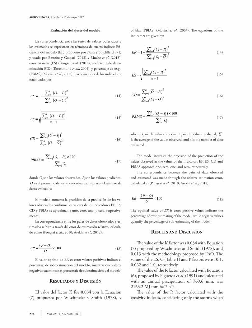
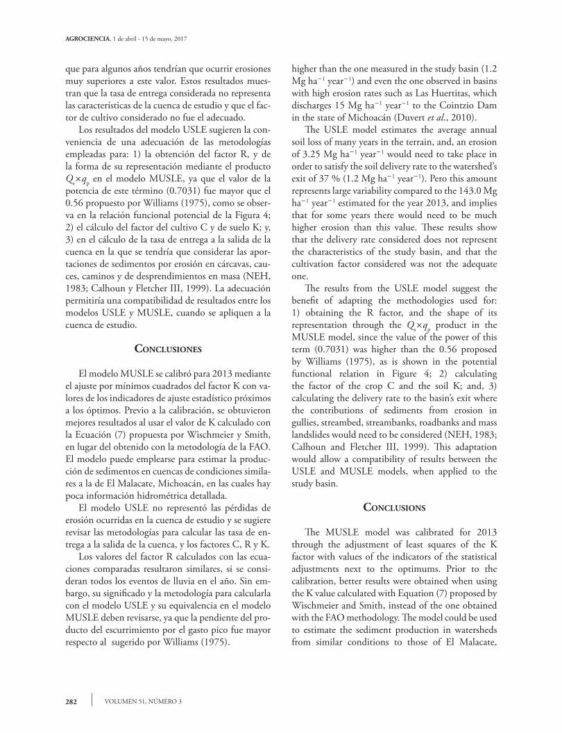
La información cartográfica usada fue modelo digital de ele-vaciones (MED), mapa de usos del suelo y vegetación, y mapa del tipo de suelo del INEGI a escala 1:50 000. El mapa de usos del suelo y vegetación se verificó en campo y se identificó un predominio del uso forestal. Para verificar el tipo de suelo se hizo un recorrido por toda la cuenca encontrándose un tipo de suelo Luvisol nítico según la clasificación FAO-UNESCO, compuesto de cuatro capas, cuya capa superficial tiene un espesor de 25 cm de textura franco arcillo limosa (32.5 de arcilla, 51.3 de limo y 6.09 % de arena muy fina) y estructura granular fina con 4.98 % de materia orgánica. La precipitación diaria de 2013 se registró, aforada en in-tervalos de 0.2 mm con un pluviógrafo HOBO RG3-M, con un total anual de 769.6 mm. Además se usaron los hidrogramas (Figura 1) y la cantidad de sedimentos a la salida de la cuenca, obtenidos de 14 eventos de escurrimiento registrados en 2013. Los hidrogramas se obtuvieron mediante un aforador de gargan-ta larga instrumentado con un sensor ultrasónico para la medi-ción del tirante y un sistema automatizado para el registro de la información. La producción de sedimentos se obtuvo al cuanti-ficar la cantidad de sólidos en suspensión de muestras tomadas a la salida de la cuenca durante los escurrimientos.

Modelos de estimación de la producción de sedimentos

Modelo USLE

La ecuación universal de pérdida de suelo (USLE) fue pro-puesta para calcular la erosión laminar y en canalillos (Wisch-meier y Smith, 1978) y está definida como:

Figura 1. Hidrogramas de los eventos de escurrimiento en el 2013.Figure 1. Hydrographs of the runoff events in 2013.

of forest use was identified. To verify the type of soil, a visit was carried out along the watershed, and the type of soil nitic Luvisol was found, based on the FAO-UNESCO classification, made up of four layers, with a superficial layer of 25 cm of loam clay sand texture (32.5 of clay, 51.3 of loam, and 6.09 % of very fine sand), and fine granular structure with 4.98 % of organic matter. The daily precipitation in 2013 was recorded, appraised at intervals of 0.2 mm with a HOBO RG3-M pluviograph, with an annual total of 769.6 mm. The hydrographs were also used (Figure 1), as well as the amount of sediments at the exit of the basin, obtained from 14 runoff events recorded in 2013. The hydrographs were obtained through a long-throated flume with an ultrasonic sensor to measure the water depth, and an automatized system to record the information. The sediment production was obtained by quantifying the amount of solids in suspension from samples taken at the exit of the basin during the runoffs.

Estimation models in the production of sediments

USLE Model The Universal Soil Loss Equation (USLE) was proposed to compute longtime average soil losses from sheet and rill erosion under specified conditions (Wischmeier and Smith, 1978), and is defined as: A=RKLSCP (1)

where, according to the international metric system of units (Foster et al. 1981), A is the annual erosion rate per unit of area (Mg ha-1 year-1), R is the rainfall and runoff erosivity factor (MJ mm ha-1 h-1 year-1), K is the soil erodibility factor (Mg ha-1 MJ-1 mm-1), L is the slope length factor (dimensionless),

A) Ocurridos por la mañana B) Ocurridos por la tarde

09-ago27-ago08-sep24-sep

0.30

0.25

0.20

0.15

0.10

0.05

0.00

00:0

0

01:0

0

02:0

0

03:0

0

04:0

0

05:0

0

06:0

0

07:0

0

08:0

0

09:0

0

10:0

0

11:0

0

12:0

0

Hora del día

Gas

to (m

3 s1 )

23-may29-jul15-ago24-ago27-ago07-sep15-sep04-oct19-oct02-nov

0.550.500.450.400.350.300.250.200.150.100.050.00

14:0

0

15:0

0

16:0

0

17:0

0

18:0

0

19:0

0

20:0

0

21:0

0

22:0

0

23:0

0

00:0

0

Hora del día

Gas

to (m

3 s1 )



A=RKLSCP (1)

donde, y de acuerdo con el sistema métrico internacional de unidades (Foster et al. 1981), A es la tasa de erosión anual por unidad de área (Mg ha-1 año-1), R es el factor de erosividad de la lluvia (MJ mm ha-1 h-1 año-1), K es el factor de erosionabili-dad del suelo (Mg ha-1 MJ-1 mm-1), L es un factor de longitud de la pendiente (adimensional), S es un factor del grado de la pendiente (adimensional), C es un factor de cultivo y manejo del cultivo (adimensional), y P es un factor de prácticas de manejo (adimensional).

Modelo MUSLE

El modelo MUSLE (Williams, 1975) es una modificación al modelo USLE, consiste en reemplazar el factor R de la erosivi-dad de la lluvia por el escurrimiento superficial y el caudal pico de una tormenta, con la finalidad de calcular la producción de sedimentos por evento y se expresa como:

Y=11.8(Qs´qp)0.56 KLSCP (2)

donde Y es la producción de sedimentos en un evento determina-do (Mg evento-1), Qs es el volumen escurrido (m3) y qp es el gasto pico del evento (m3 s-1).

Cálculo de los factores de la USLE y MUSLE

Los volúmenes escurridos y los gastos pico se obtuvieron de los hidrogramas medidos. Se calcularon los valores promedio de los factores K, R, LS, C y P. El factor P de prácticas de manejo se consideró igual a la unidad porque no se realizan prácticas de conservación. El factor K se calculó usando un solo tipo de suelo con la información reportada en datos experimentales, el factor R se obtuvo con los datos de la lluvia, y los factores LS y C se obtuvieron de forma ponderada por el área (Sadeghi et al., 2007; Pongsai et al., 2010) mediante el procesamiento del MED y del mapa de uso de suelos y vegetación con ArcGis versión 10.1, cuyos procedimientos de cálculo se describen a continuación.

Factor R

Este factor representa la capacidad potencial que tienen las gotas de agua de lluvia para causar erosión y se calculó de dos for-mas: mediante el índice EI30 (Wischmeier y Smith, 1978), y con una ecuación adaptada por Figueroa et al. (1991) que considera una relación funcional de tipo cuadrática con la precipitación media anual registrada.

S is slope steepness factor (dimensionless), C is the cropping management factor (dimensionless), and P is the support practice factor (dimensionless).

MUSLE model

The MUSLE model (Williams, 1975) is a modification of the USLE model, and it consists in replacing the R factor of erosivity of the rain because of superficial runoff and the peak runoff rate of a storm, with the aim of calculating the sediment yield per event and expressed as: Y=11.8(Qs´qp)

0.56 KLSCP (2)

where Y is the sediment yield in a specific event (Mg event-1), Qs is the runoff volume (m3) and qp is the peak runoff rate of the event (m3 s-1).

Calculation of the factors from USLE and MUSLE

The runoff volumes and the peak runoff rate were obtained from the hydrographs measured. The average values of the K, R, LS, C and P factors were calculated. The P erosion control practice factor was considered equal to the unit because conservation practices were not performed. The K factor was calculated by employing a single type of soil with the information reported in the experimental data, the R factor was obtained with data from rain, and the LS and C factors were obtained in a weighted form by the area (Sadeghi et al., 2007; Pongsai et al., 2010), through the processing of MED and the map of land and vegetation uses with ArcGis version 10.1, whose procedures for calculation are described next.

R factor

This factor represents the potential capacity that rain drops have to cause erosion and it was calculated in two ways: through the EI30 index (Wischmeier and Smith, 1978), and with an equation adapted by Figueroa et al. (1991), who consider a quadratic functional relationship with the mean annual precipitation registered. The EI30 method was used because there is daily information about precipitation, registered at intervals of minutes. This method is defined as the product of the total kinetic energy of a rain event by the maximum intensity in 30 min, so that the total value of the factor of the rain erosivity R is the sum of values of erosivity of individual storms, calculated as follows: (Wischmeier and Smith, 1978):



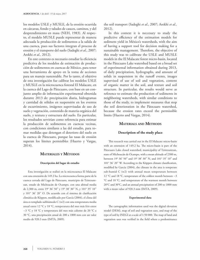
El método EI30 se usó porque hay información diaria de la precipitación, registrada a intervalos de minutos. Este método es el producto de la energía cinética total de un evento de lluvia por la intensidad máxima en 30 min, de manera que el valor total del factor de erosividad de la lluvia R es la suma de valores de erosividad de tormentas individuales, calculado así (Wischmeier y Smith, 1978):

R EI iin

== ( )301 (3)

donde E es la energía cinética de la lluvia de cada tormenta (MJ ha-1 mm-1), I30 es la intensidad máxima de la lluvia en cuales-quiera 30 min de cada tormenta (mm h-1), y n es el número de tormentas en el año.

La energía cinética de cada tormenta es la suma de las ener-gías cinéticas de los intervalos de lluvia, diferenciados por sus intensidades de lluvia, y se calculó con la ecuación propuesta por Wischmeier and Smith (1978):

E e ppjjn

j= ´= 1 (4)

ej=0.119+0.0873log10(Ij) (5)

donde ej es la energía cinética del intervalo de lluvia j de una tormenta (MJ ha-1 mm-1), y Ij es la intensidad de la lluvia del in-tervalo j (mm h-1), y ppj es la precipitación del intervalo j (mm). Para intensidades mayores de 76 mm h-1 se estableció un valor de e de 0.283.

De acuerdo con el criterio de cálculo del EI30 propuesto por Wischmeier y Smith (1978), no se consideraron las tormentas con precipitaciones menores de 12.5 mm con periodos de lluvia separados más de 6 h, a menos que la precipitación fuera 6.2 mm o más en 15 min (I15³24.8 mm h-1). La existencia de los perio-dos de lluvia en las tormentas largas se definieron cuando en un lapso de 6 h lámina fue menor a 1.2 mm (Renard et al., 1997). El factor R se calculó con la ecuación adaptada por Figueroa et al. (1991) como una alternativa metodológica a las cuencas donde no es posible calcular el EI30 por falta de información de-tallada de la precipitación a lo largo del año. La cuenca de estudio se localiza en la zona hidrológica V (Bravo et al., 2009a) y la ecuación:

R=3.488P-0.00088P2 (6)

donde P es la precipitación anual de 2013 en milímetros.

R EI iin

== ( )301 (3)

where E is the kinetic energy of the rain from each storm (MJ ha-1 mm-1), I30 is the maximum intensity of rain in any 30 min from each storm (mm h-1), and n is the number of storms in the year.

The kinetic energy of each storm is the eddition of the kinetic energies of the rain intervals, differentiated by their rain intensities, and it was calculated with the equation proposed by Wischmeier and Smith (1978): E e ppjj

nj= ´

= 1 (4) ej=0.119+0.0873log10(Ij) (5)

where ej is the kinetic energy of the interval of rain j of a storm (MJ ha-1 mm-1), and Ij is the intensity of the rain from interval j (mm h-1), and ppj is the precipitation of the interval j (mm). For intensities greater than 76 mm h-1 an e value of 0.283 was established.

According to the criterion to calculate EI30 proposed by Wischmeier and Smith (1978), the storms with precipitations lower than 12.5 mm with rain periods separated more than 6 h were not considered, unless 6.2 mm or more had fallen in 15 min (I15³24.8 mm h-1). The existence of rain periods in long storms was defined when the sheet was less than 1.2 mm in a lapse of 6 h (Renard et al., 1997). The R factor is calculated with the equation adapted by Figueroa et al. (1991) as a methodological alternative to the watersheds where it is not possible to calculate the EI30 for lack of detailed information from the precipitation throughout the year. The watershed of study is located in the hydrological zone V (Bravo et al., 2009a), with the following equation: R=3.488P-0.00088P2 (6)

where P is the annual precipitation of 2013 in millimeters.

K factor

The term erodibility of the soil is used to indicate the susceptibility of a soil to erosion. It is defined as the rate of soil loss for each additional unit of EI30 when the slope and its length, the plant cover, and the conservation practices of the soil remain constant and its values are equal to one (Wischmeier and Smith, 1978).



Factor K

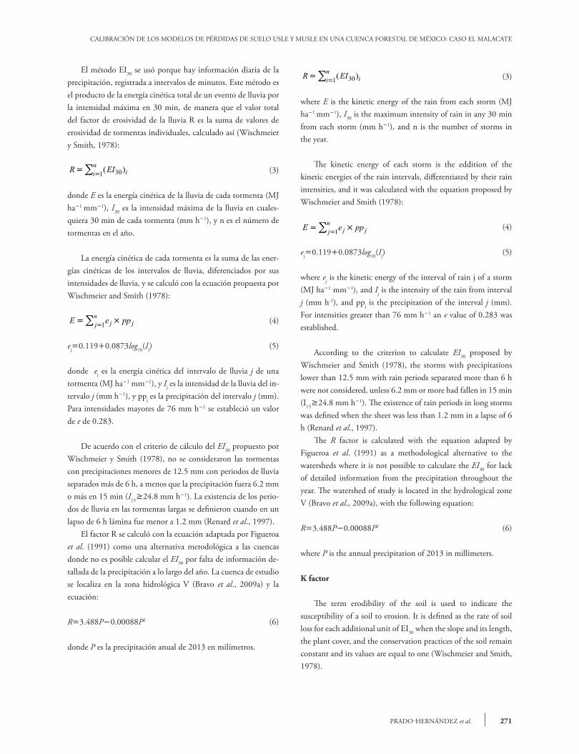
El término erosionabilidad del suelo se utiliza para indicar la susceptibilidad de un suelo a la erosión. Se define como la tasa de pérdida de suelo por cada unidad adicional de EI30 cuando la pendiente y su longitud, la cobertura vegetal y las prácticas de conservación del suelo permanecen constantes y sus valores son iguales a uno (Wischmeier y Smith, 1978). Como la suma de las partículas del limo más la de arena muy fina fue menos de 70 % del total de las partículas del suelo, el factor K se calculó con la ecuación propuesta por Wischmeier y Smith (1978):

KM MO

= ´- +L

NMM

013130 0021 12

100

114.

. ( ).

(7)3 25 2 2 5 3

100. ( ) . ( )C Cestr perm- + - O

QP

donde M es un parámetro de tamaño de partícula, MO es el por-centaje de materia orgánica (%), Cestr es un código de estructura del suelo, Cperm es un código de permeabilidad del suelo, y 0.313 es un factor de conversión del sistema de unidades inglés al mé-trico internacional (Foster et al, 1981). El parámetro de tamaño de partícula se calculó como:

M=(ml+mamf)(100-ma) (8)

donde ml es el porcentaje de contenido de limo (diámetro de partículas de 0.002 a 0.05 mm), mamf porcentaje del contenido de arena muy fina (diámetro de 0.05 a 0.10 mm), y ma es el por-centaje del contenido de arcilla (diámetro de partículas menores de 0.002 mm). El valor de la permeabilidad del suelo se determinó en fun-ción de su textura empleando las relaciones funcionales descritas por Saxton y Rawls (2006). Otro método usado fue el de la FAO (1980) usado en Méxi-co, ya que el factor K se determina solo en función de la unidad a la cual pertenece el suelo en la clasificación FAO-UNESCO y de la textura de la capa superficial.

Factor LS

Este factor representa el efecto de la topografía sobre la ero-sión del suelo. La erosión aumenta conforme se incrementa la longitud del terreno (L) en el sentido de la pendiente y la inclina-ción de la superficie (S) se hace mayor, calculados como (Wisch-meier y Smith, 1978):

As the sum of the loam particles plus the very fine sand was less than 70 % of the total of soil particles, the K factor was calculated with the equation proposed by Wischmeier and Smith (1978):

KM MO

= ´- +L

NMM

013130 0021 12

100

114.

. ( ).

(7)3 25 2 2 5 3

100. ( ) . ( )C Cestr perm- + - O

QP

where M is a parameter of the particle size, MO is the percentage of organic matter (%), Cestr is a code of soil structure, Cperm is a code of soil permeability, and 0.313 is a conversion factor of the system of English units to the international metric system (Foster et al, 1981). The parameter of the particle size was calculated as: M=(ml+mamf)(100-ma) (8)

where ml is the percentage of loam content (diameter of particles of 0.002 to 0.05 mm), mamf is the percentage of the content of very fine sand (diameter of 0.05 to 0.10 mm), and ma is the percentage of the content of clay (diameter of particles smaller than 0.002 mm). The value of the soil permeability was determined in function of their texture using the functional relations described by Saxton and Rawls (2006). Another method was that of FAO (1980), which is used in México, since the K factor is determined only in function of the unit to which the soil belongs in the FAO-UNESCO classification and of the texture of the superficial layer.

LS factor

This factor represents the effect of the topography on soil erosion. The erosion increases as the length (L) of the plot increases in the direction of the slope, and the inclination of the surface (S) increases, calculated as (Wischmeier and Smith, 1978):

LS s sm

=FHG

IKJ + +

22 13

0 065 0 045 0 0065 2.

. . .d i (9)

where:

LSm

=FHG

IKJ

22 13.

(10)



LS s sm

=FHG

IKJ + +

22 13

0 065 0 045 0 0065 2.

. . .d i (9)

donde:

LSm

=FHG

IKJ

22 13. (10)

S=0.065+0.045s+0.0065s2 (11)

donde es la longitud de la pendiente (m), s es la pendiente del terreno (%), y el exponente m del factor de la longitud de pen-diente considera la proporción de erosión causada por la erosión entre canalillos, debida al impacto de las gotas y la causada en ca-nalillos por la fuerza de arrastre del flujo (Renard et al., 1997). El valor de m varía en función de la pendiente del terreno y se calcu-ló con la ecuación propuesta por McCool (Renard et al., 1997):

m=+ +

sin. sin . sin .

0 05 0 269 0 8 (12)

donde es el ángulo de la pendiente.

La ecuación clásica para calcular el factor LS, propuesta por Wiscmeier y Smith (1978), no representa bien el efecto de la topografía en la erosión del suelo para pendientes mayores de 16 % (Pongsai et al., 2010), por lo cual el factor S se calculó con la ecuación propuesta por McCool (Renard et al., 1997) para pen-dientes mayores a 9 %:

S=16.8 sin -0.5 (13)

donde es el ángulo de la pendiente.

Factor C

El factor C de manejo de cultivo y cobertura del suelo es la relación de pérdidas de un terreno cultivado en condiciones específicas, con respecto a las pérdidas de un suelo desnudo y con barbecho continuo en las mismas condiciones de suelo, pendien-te y lluvia (Wischmeier y Smith, 1978). Para su cálculo se empleó la metodología y los valores pro-puestos por Wischmeier y Smith (1978). En la agricultura de temporal, donde se siembra maíz de manera preponderante, se cuantificó mediante los índices de erosividad EI30 en cada una de las etapas del cultivo y las pérdidas relativas de suelo en áreas de cultivo en relación a terrenos bajo barbecho continuo.

S=0.065+0.045s+0.0065s2 (11)

where is the plot slope length (m), s is the slope of the plot (%), and the m exponent of the factor of the slope length considers the proportion of erosion caused by the erosion between drains, due to the impact of the drops, and that caused in drains by the dragging force of the flow (Renard et al., 1997). The value of m varies in function of the slope of the plot and was calculated with the equation proposed by McCool (Renard et al., 1997):

m=

+ +

sin. sin . sin .

0 05 0 269 0 8 (12)

where is the angle of slope.

The classical equation to calculate the LS factor, proposed by Wischmeier and Smith (1978), does not represent well the effect of the topography on the soil erosion for slopes greater than 16 % (Pongsai et al., 2010), so that the S factor was calculated with the equation proposed by McCool (Renard et al., 1997) for slopes greater than 9 %: S=16.8 sin -0.5 (13)

where is the angle of the slope.

C factor

The C Factor of crop management and soil cover is the relationship of losses in a plot cultivated under specific conditions, with regards to the losses of naked soil and with continuous fallow under the same conditions of soil, slope and rain (Wischmeier and Smith, 1978). For its calculation, the methodology and values proposed by Wischmeier and Smith (1978) were used. In rainfed agriculture, where maize is sown predominantly, it was quantified through the erosivity indexes EI30 in each one of the stages of cultivation and the relative soil losses in cultivation areas compared to lands under continuous fallow.

Evaluation of the model’s adjustment

The correspondence between the series of values observed and those estimated are expressed in terms of four indexes: Model’s efficiency (EF) proposed by Nash and Sutcliffe (1971) and used by Besteiro and Gaspari (2012), and Muche et al. (2013); standard error (ES) (Pongsai et al. (2010); coefficient of determination (CD) (Rosenmund et al., 2005); and percentage



Evaluación del ajuste del modelo

La correspondencia entre las series de valores observados y los estimados se expresaron en términos de cuatro índices: Efi-ciencia del modelo (EF) propuesto por Nash y Sutcliffe (1971) y usado por Besteiro y Gaspari (2012) y Muche et al. (2013); error estándar (ES) (Pongsai et al. (2010); coeficiente de deter-minación (CD) (Rosenmund et al., 2005); y porcentaje de sesgo (PBIAS) (Moriasi et al., 2007). Las ecuaciones de los indicadores están dadas por:

EFO P

O O

i iin

iin

= --

-

=

=

1

21

21

a fb g

(14)

ESO P

ni ii

n

=-

-= a f21

1 (15)

CDO P

O O

iin

iin

=-

-

=

=

b gb g

21

21

(16)

PBIASO P

Oi ii

n

iin=- ´

=

=

a f 1001

1 (17)

donde Oi son los valores observados, Pi son los valores predichos, O es el promedio de los valores observados, y n es el número de datos evaluados.

El modelo aumenta la precisión de la predicción de los va-lores observados conforme los valores de los indicadores EF, ES, CD y PBIAS se aproximan a uno, cero, uno, y cero, respectiva-mente. La correspondencia entre los pares de datos observados y es-timados se hizo a través del error de estimación relativo, calcula-do como (Pongsai et al., 2010; Arekhi et al., 2012):

ERP O

O=

- ´100 (18)

El valor óptimo de ER es cero; valores positivos indican el porcentaje de sobreestimación del modelo, mientras que valores negativos cuantifican el porcentaje de subestimación del modelo.

ResultAdos y dIscusIón

El valor del factor K fue 0.034 con la Ecuación (7) propuesta por Wischmeier y Smith (1978), y

of bias (PBIAS) (Moriasi et al., 2007). The equations of the indicators are given by:

EF

O P

O O

i iin

iin

= --

-

=

=

1

21

21

a fb g

(14)

ESO P

ni ii

n

=-

-= a f21

1 (15)

CD

O P

O O

iin

iin

=-

-

=

=

b gb g

21

21

(16)

PBIAS

O P

Oi ii

n

iin=- ´

=

=

a f 1001

1 (17)

where Oi are the values observed, Pi are the values predicted, O is the average of the values observed, and n is the number of data evaluated.

The model increases the precision of the prediction of the values observed as the values of the indicators EF, ES, CD and PBIAS approach one, zero, one, and zero, respectively. The correspondence between the pairs of data observed and estimated was made through the relative estimation error, calculated as (Pongsai et al., 2010; Arekhi et al., 2012): ER

P OO

=-

´100 (18)

The optimal value of ER is zero; positive values indicate the percentage of over-estimating of the model, while negative values quantify the percentage of sub-estimating of the model.

Results And dIscussIon

The value of the K factor was 0.034 with Equation (7) proposed by Wischmeier and Smith (1978), and 0.013 with the methodology proposed by FAO. The values of the LS, C (Table 1) and P factors were 10.1, 0.062 and 1.0, respectively. The value of the R factor calculated with Equation (6), proposed by Figueroa et al. (1991) and calculated with an annual precipitation of 769.6 mm, was 2163.2 MJ mm ha-1 h-1. The value of the R factor calculated with the erosivity indexes, considering only the storms when



0.013 con la metodología propuesta por la FAO. Los valores de los factores LS, C (Cuadro 1) y P fueron 10.1, 0.062 y 1.0, respectivamente. El valor del factor R calculado con la Ecuación (6), propuesta por Figueroa et al. (1991) y calcula-do con una precipitación anual de 769.6 mm, fue 2163.2 MJ mm ha-1 h-1. El valor del factor R calculado con los índices de erosividad, considerando solo las tormentas en las cuales hubo escurrimientos y que cumplieron con los criterios de Wischmeier y Smith (1978), fue 1154.9 MJ mm ha-1 h-1 año-1 (Cuadro 2). Este resultado correspondió a la suma de eventos de lluvia con lámi-nas precipitadas mayores que 12.5 mm o con láminas inferiores a 12.5 mm, pero con intensidades de lluvia superiores que 24.8 mm h-1 en cualesquiera 15 min (I15). Las tormentas del 8 y 24 de septiembre produ-jeron arrastre de sedimentos pero no se consideraron por no cumplir con los criterios establecidos, ya que se presentaron precipitaciones inferiores a 12.5 mm y I15 inferiores a 24.8 mm h-1. En las tormentas del 23 de mayo y 27 de agosto se presentaron dos periodos de lluvia, y solo uno de ellos cumplió los requisitos para tomarse en cuenta en el EI30.

there were runoffs and which fulfilled the criteria of Wischmeier and Smith (1978), was 1154.9 MJ mm ha-1 h-1 year-1 (Table 2). This result corresponded to the sum of rain events with precipitated sheets greater than 12.5 mm or with sheets lower than 12.5 mm, but with rain intensities above 24.8 mm h-1 in any 15 min (I15). The storms of September 8 and

Cuadro 1. Valores del factor C de acuerdo con el uso del suelo y vegetación en la cuenca El Malacate, Michoacán.

Table 1. Values of the C factor according to the land and plant use in the El Malacate watershed, Michoacán.

Uso de suelo Superficie (ha)

Porcentaje (%)

Factor C

Agricultura de temporal (maíz) 1.77 1.19 0.555

Áreas sin vegetación 7.37 4.94 1.000Pastizal forestal erosionado 2.74 1.84 0.071Forestal 91.31 61.18 0.001Forestal-pastizal 19.39 12.99 0.011Pastizal-forestal 24.86 16.66 0.010Reforestación-zonas erosionadas 1.80 1.20 0.065

Cuadro 2. Índices de erosividad EI30 de las tormentas con eventos de escurrimiento del año 2013.Table 2. Erosivity index EI30 of the storms with runoff events in 2013.

Fecha Precipitación(mm)

I15(mm h-1)

I30(mm h-1)

EI30(MJ mm ha-1 h-1)

23/05† 3.80 12.509.00 25.36 14.93 30.77

29/07 26.40 29.45 188.4109/08 18.60 27.80 123.7515/08 19.20 21.73 92.3324/08 27.60 32.82 218.93

27/08† 25.20 11.89 53.894.60 9.68

07/09 30.00 10.77 86.7608/09 2.40 3.1315/09 35.80 10.75 63.33

24/09† 10.60 11.451.20 4.90

04/10 16.80 43.47 186.6919/10 12.00 31.67 27.04 71.5202/11 13.20 13.54 38.55Total 1154.90

†Hubo dos periodos de lluvia en la tormenta. v There were two rain periods in the storm.



Calibración del modelo MUSLE

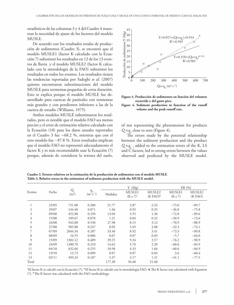
Las Figuras 2 y 3 muestran una relación potencial entre la producción de sedimentos y los volúmenes escurridos y caudales pico de cada tormenta de acuer-do con Williams (1975). El ajuste de estas relaciones fue R2>0.95, pero las desviaciones estándar fueron altas; al relacionar la producción de sedimentos con el volumen escurrido superficialmente, el error es-tándar fue 8.2, y 6.6 Mg cuando dependió del gasto pico, como lo reportan Sadeghi et al. (2007). Al relacionar la producción de sedimentos con el producto del escurrimiento superficial por el gasto pico, término por el cual Williams (1975) sustitu-yó el factor de erosividad de la lluvia R de la USLE, hay un buen ajuste en un modelo de tipo potencial (R2=0.983; Figura 4). Sin embargo, el valor de la potencia (0.703) es superior al encontrado por Wi-lliams (1975) en EE. UU. (0.56) y el error estándar fue 4.4 Mg. Un modelo de tipo lineal también pre-sentó ajuste R2=0.945 con un error estándar inferior al de tipo potencial (3.1 Mg), pero con la desventaja de no representar el fenómeno para productos Qs´qp cercanos a cero (Figura 4). Los errores cometidos por la relación potencial en-tre la producción de sedimentos y el producto Qs´qp, sumados a los errores de estimación de los factores K, LS, y C, condujeron a errores fuertes entre los valores observados y predichos por el modelo MUSLE. En efecto, los resultados del Cuadro 3 y los indicadores

24 produced sediment dragging but they were not considered because they did not comply with the criteria established, since precipitations of less than 12.5 mm took place and I15 lower than 24.8 mm h-1. In the storms of May 23 and August 27, there were two rain periods, and only one of them fulfilled the requirements to be taken into account in the EI30.

Calibration of the MUSLE model

Figures 2 and 3 show a potential relationship between the production of sediments and the runoff volumes and peak runoff rate of each storm, as Williams (1975) points out. The adjustment of these relationships was R2>0.95, but the standard deviations were high; when relating the sediment production with the runoff volume, the standard error was 8.2 and 6.6 Mg when it depended on the peak expenditure, as Sadeghi et al. (2007) reported.

When relating the production of sediments with the product of the runoff volume by the peak runoff rate, term by which Williams (1975) substituted the erosivity factor of R rain of the USLE, there is good adjustment in a potential-type model (R2=0.983; Figure 4). However, the value of the power (0.703) is higher than the one found by Williams (1975) in the US (0.56), and the standard error was 4.4 Mg. A model of linear type also presented an adjustment R2=0.945 with a lower standard error to the potential type (3.1 Mg), but with the disadvantage

Figura 2. Producción de sedimentos en función del volumen escurrido.

Figure 2. Sediment production in function of the runoff volume.

Figura 3. Producción de sedimentos en función del gasto pico.

Figure 3. Sediment production in function of the peak runoff rate.

504540353025201510

50

0 500 1000 1500 2000 2500

Prod

ucci

ón d

e se

dim

ento

s Y(M

g)

Volumen escurrido Qs (m3)

Y0.003Qs1.2833

R20.956

4540353025201510

500.0 0.1 0.2 0.3 0.4 0.5 0.6

Gasto pico qp (m3 s1)

Prod

ucci

ón d

e se

dim

ento

s Y (M

g)

Y91.769qp1.4787

R20.966



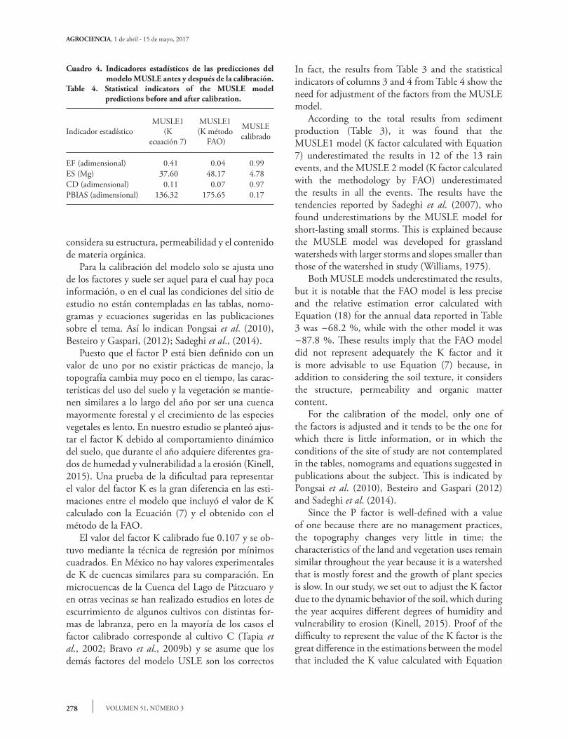
estadísticos de las columnas 3 y 4 del Cuadro 4 mues-tran la necesidad de ajuste de los factores del modelo MUSLE. De acuerdo con los resultados totales de produc-ción de sedimentos (Cuadro 3), se encontró que el modelo MUSLE1 (factor K calculado con la Ecua-ción 7) subestimó los resultados en 12 de los 13 even-tos de lluvia y el modelo MUSLE2 (factor K calcu-lado con la metodología de la FAO) subestimó los resultados en todos los eventos. Los resultados tienen las tendencias reportadas por Sadeghi et al. (2007) quienes encontraron subestimaciones del modelo MUSLE para tormentas pequeñas de corta duración. Esto se explica porque el modelo MUSLE fue de-sarrollado para cuencas de pastizales con tormentas más grandes y con pendientes inferiores a las de la cuenca de estudio (Williams, 1975). Ambos modelos MUSLE subestimaron los resul-tados, pero es notable que el modelo FAO sea menos preciso y el error de estimación relativo calculado con la Ecuación (18) para los datos anuales reportados en el Cuadro 3 fue -68.2 %, mientras que con el otro modelo fue -87.8 %. Estos resultados implican que el modelo FAO no representó adecuadamente el factor K y es más recomendable usar la Ecuación (7) porque, además de considerar la textura del suelo,

of not representing the phenomenon for products Qs´qp close to zero (Figure 4). The errors made by the potential relationship between the sediment production and the product Qs´qp , added to the estimation errors of the K, LS and C factors, led to strong errors between the values observed and predicted by the MUSLE model.

Figura 4. Producción de sedimentos en función del volumen escurrido y del gasto pico.

Figure 4. Sediment production in function of the runoff volume and the peak runoff rate.

Cuadro 3. Errores relativos en la estimación de la producción de sedimentos con el modelo MUSLE.Table 3. Relative errors in the estimation of sediment production with the MUSLE model.

Evento Fecha Qs(m3)

qp(m3 s-1)

Y (Mg) ER (%)

Medidos MUSLE1(K e 7)†

MUSLE2(K FAO)¶

MUSLE1(K e 7)

MUSLE2(K FAO)

1 23/05 731.00 0.380 21.77 5.87 2.24 -73.0 -89.72 29/07 144.40 0.071 1.46 0.92 0.35 -36.8 -75.83 09/08 452.88 0.250 13.04 3.55 1.36 -72.8 -89.64 15/08 109.67 0.078 1.21 0.84 0.32 -30.9 -73.65 24/08 942.00 0.530 27.98 8.15 3.12 -70.9 -88.96 27/08 985.80 0.247 8.05 5.45 2.08 -32.3 -74.17 07/09 2044.34 0.287 33.40 8.92 3.41 -73.3 -89.88 08/09 16.55 0.006 0.07 0.07 0.03 -5.7 -64.09 15/09 1302.12 0.489 39.25 9.34 3.57 -76.2 -90.9

10 24/09 1280.70 0.210 14.62 5.76 2.20 -60.6 -84.911 04/10 632.66 0.255 10.98 4.33 1.66 -60.6 -84.912 19/10 12.73 0.009 0.07 0.07 0.03 3.6 -60.413 02/11 493.24 0.187 5.37 3.17 1.21 -41.1 -77.5

Total 177.30 56.40 21.60

†El factor K se calculó con la Ecuación (7). ¶ El factor K se calculó con la metodología FAO. v The K factor was calculated with Equation (7). ¶ The K factor was calculated with the FAO methodology.

4540353025201510

50

0 100 200 300 400 500 600 700

Prod

ucci

ón d

e se

dim

ient

os Y

(Mg)

Qsqp (m6 s1)

Y0.057(Qsqp)0.914R20.945

Y0.318(Qsqp)0.7031

R2=0.983



considera su estructura, permeabilidad y el contenido de materia orgánica. Para la calibración del modelo solo se ajusta uno de los factores y suele ser aquel para el cual hay poca información, o en el cual las condiciones del sitio de estudio no están contempladas en las tablas, nomo-gramas y ecuaciones sugeridas en las publicaciones sobre el tema. Así lo indican Pongsai et al. (2010), Besteiro y Gaspari, (2012); Sadeghi et al., (2014). Puesto que el factor P está bien definido con un valor de uno por no existir prácticas de manejo, la topografía cambia muy poco en el tiempo, las carac-terísticas del uso del suelo y la vegetación se mantie-nen similares a lo largo del año por ser una cuenca mayormente forestal y el crecimiento de las especies vegetales es lento. En nuestro estudio se planteó ajus-tar el factor K debido al comportamiento dinámico del suelo, que durante el año adquiere diferentes gra-dos de humedad y vulnerabilidad a la erosión (Kinell, 2015). Una prueba de la dificultad para representar el valor del factor K es la gran diferencia en las esti-maciones entre el modelo que incluyó el valor de K calculado con la Ecuación (7) y el obtenido con el método de la FAO. El valor del factor K calibrado fue 0.107 y se ob-tuvo mediante la técnica de regresión por mínimos cuadrados. En México no hay valores experimentales de K de cuencas similares para su comparación. En microcuencas de la Cuenca del Lago de Pátzcuaro y en otras vecinas se han realizado estudios en lotes de escurrimiento de algunos cultivos con distintas for-mas de labranza, pero en la mayoría de los casos el factor calibrado corresponde al cultivo C (Tapia et al., 2002; Bravo et al., 2009b) y se asume que los demás factores del modelo USLE son los correctos

In fact, the results from Table 3 and the statistical indicators of columns 3 and 4 from Table 4 show the need for adjustment of the factors from the MUSLE model. According to the total results from sediment production (Table 3), it was found that the MUSLE1 model (K factor calculated with Equation 7) underestimated the results in 12 of the 13 rain events, and the MUSLE 2 model (K factor calculated with the methodology by FAO) underestimated the results in all the events. The results have the tendencies reported by Sadeghi et al. (2007), who found underestimations by the MUSLE model for short-lasting small storms. This is explained because the MUSLE model was developed for grassland watersheds with larger storms and slopes smaller than those of the watershed in study (Williams, 1975). Both MUSLE models underestimated the results, but it is notable that the FAO model is less precise and the relative estimation error calculated with Equation (18) for the annual data reported in Table 3 was -68.2 %, while with the other model it was -87.8 %. These results imply that the FAO model did not represent adequately the K factor and it is more advisable to use Equation (7) because, in addition to considering the soil texture, it considers the structure, permeability and organic matter content. For the calibration of the model, only one of the factors is adjusted and it tends to be the one for which there is little information, or in which the conditions of the site of study are not contemplated in the tables, nomograms and equations suggested in publications about the subject. This is indicated by Pongsai et al. (2010), Besteiro and Gaspari (2012) and Sadeghi et al. (2014). Since the P factor is well-defined with a value of one because there are no management practices, the topography changes very little in time; the characteristics of the land and vegetation uses remain similar throughout the year because it is a watershed that is mostly forest and the growth of plant species is slow. In our study, we set out to adjust the K factor due to the dynamic behavior of the soil, which during the year acquires different degrees of humidity and vulnerability to erosion (Kinell, 2015). Proof of the difficulty to represent the value of the K factor is the great difference in the estimations between the model that included the K value calculated with Equation

Cuadro 4. Indicadores estadísticos de las predicciones del modelo MUSLE antes y después de la calibración.

Table 4. Statistical indicators of the MUSLE model predictions before and after calibration.

Indicador estadísticoMUSLE1

(K ecuación 7)

MUSLE1(K método

FAO)

MUSLE calibrado

EF (adimensional) 0.41 0.04 0.99ES (Mg) 37.60 48.17 4.78CD (adimensional) 0.11 0.07 0.97PBIAS (adimensional) 136.32 175.65 0.17



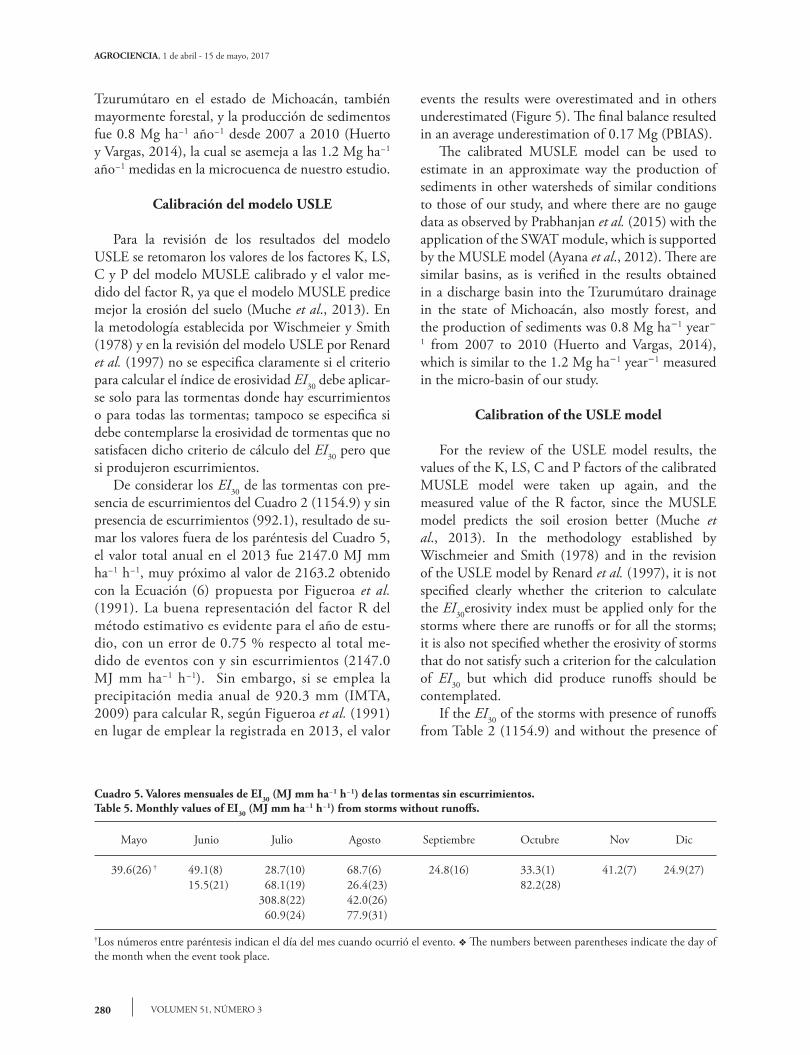
y calculados con la metodología propuesta por Wis-chmeier y Smith (1978). En el Cuadro 4 se observa que los valores de tres (EF, CD y PBIAS) de los cua-tro indicadores estadísticos de ajuste son muy próxi-mos a sus óptimos. El valor próximo a la unidad del indicador de Nash y Sutcliffe (EF) establece que el modelo calibrado es eficiente. El valor de ES impli-ca que existió un error estándar de 4.78 Mg en la producción de sedimentos y dadas las 149.2 ha de la cuenca, se traduce en un error estándar de 0.03 Mg ha-1. El valor de CD próximo a la unidad indica que los valores predichos siguieron la tendencia de los medidos, compensando los errores; así, en algunos eventos se sobrestimaron los resultados y en otros se subestimaron (Figura 5). El balance final resultó en una subestimación promedio de 0.17 Mg (PBIAS). El modelo MUSLE calibrado se puede usar para estimar de forma aproximada la producción de sedi-mentos en otras cuencas de condiciones similares a la de nuestro estudio, y donde no se disponga de datos de aforo como lo observó Prabhanjan et al. (2015) con la aplicación del módulo SWAT, el cual está so-portado por el modelo MUSLE (Ayana et al., 2012). Existen cuencas similares, como se constata en los re-sultados obtenidos en una cuenca de descarga al dren

(7), and the one obtained with the FAO method. The value of the calibrated K factor was 0.107 and was obtained through the technique of least squares regression. In México there are no experimental values of K from similar watersheds for their comparison. In micro-basins of the Pátzcuaro Lake watershed and other neighboring ones, studies were performed in runoff plots of some crops with different types of farming, but in most of the cases the calibrated factor corresponds to crop C (Tapia et al., 2002; Bravo et al., 2009b) and it is assumed that the other factors of the USLE model are the correct ones and calculated with the methodology proposed by Wischmeier and Smith (1978). Table 4 shows that the values of three (EF, CD and PBIAS) of the four statistical indicators of adjustment are quite close to their optimums. The value next to the unit of the Nash and Sutcliffe (EF) indicator establishes that the calibrated model is efficient. The ES value implies that there was a standard error of 4.78 Mg in the production of sediments and given the 149.2 ha of the watershed, it translates into a standard error of 0.03 Mg ha-1. The CD value next to the unit indicates that the values predicted suggested the trend of those measured, compensating the errors; thus, in some

Figura 5. Producción de sedimentos medidos y simulados con el modelo MUSLE calibrado.Figure 5. Sediment production measured and simulated with the calibrated MUSLE model.

40

35

30

25

20

15

10

5

01 2 3 4 5 6 7 8 9 10 11 12 13

Evento de escurrimiento

Prod

ucci

ón d

e se

dim

ento

s Y (M

g)

Medidos

Simulados



Tzurumútaro en el estado de Michoacán, también mayormente forestal, y la producción de sedimentos fue 0.8 Mg ha-1 año-1 desde 2007 a 2010 (Huerto y Vargas, 2014), la cual se asemeja a las 1.2 Mg ha-1 año-1 medidas en la microcuenca de nuestro estudio.

Calibración del modelo USLE

Para la revisión de los resultados del modelo USLE se retomaron los valores de los factores K, LS, C y P del modelo MUSLE calibrado y el valor me-dido del factor R, ya que el modelo MUSLE predice mejor la erosión del suelo (Muche et al., 2013). En la metodología establecida por Wischmeier y Smith (1978) y en la revisión del modelo USLE por Renard et al. (1997) no se especifica claramente si el criterio para calcular el índice de erosividad EI30 debe aplicar-se solo para las tormentas donde hay escurrimientos o para todas las tormentas; tampoco se especifica si debe contemplarse la erosividad de tormentas que no satisfacen dicho criterio de cálculo del EI30 pero que si produjeron escurrimientos. De considerar los EI30 de las tormentas con pre-sencia de escurrimientos del Cuadro 2 (1154.9) y sin presencia de escurrimientos (992.1), resultado de su-mar los valores fuera de los paréntesis del Cuadro 5, el valor total anual en el 2013 fue 2147.0 MJ mm ha-1 h-1, muy próximo al valor de 2163.2 obtenido con la Ecuación (6) propuesta por Figueroa et al. (1991). La buena representación del factor R del método estimativo es evidente para el año de estu-dio, con un error de 0.75 % respecto al total me-dido de eventos con y sin escurrimientos (2147.0 MJ mm ha-1 h-1). Sin embargo, si se emplea la precipitación media anual de 920.3 mm (IMTA, 2009) para calcular R, según Figueroa et al. (1991) en lugar de emplear la registrada en 2013, el valor

events the results were overestimated and in others underestimated (Figure 5). The final balance resulted in an average underestimation of 0.17 Mg (PBIAS). The calibrated MUSLE model can be used to estimate in an approximate way the production of sediments in other watersheds of similar conditions to those of our study, and where there are no gauge data as observed by Prabhanjan et al. (2015) with the application of the SWAT module, which is supported by the MUSLE model (Ayana et al., 2012). There are similar basins, as is verified in the results obtained in a discharge basin into the Tzurumútaro drainage in the state of Michoacán, also mostly forest, and the production of sediments was 0.8 Mg ha-1 year-1 from 2007 to 2010 (Huerto and Vargas, 2014), which is similar to the 1.2 Mg ha-1 year-1 measured in the micro-basin of our study.

Calibration of the USLE model

For the review of the USLE model results, the values of the K, LS, C and P factors of the calibrated MUSLE model were taken up again, and the measured value of the R factor, since the MUSLE model predicts the soil erosion better (Muche et al., 2013). In the methodology established by Wischmeier and Smith (1978) and in the revision of the USLE model by Renard et al. (1997), it is not specified clearly whether the criterion to calculate the EI30erosivity index must be applied only for the storms where there are runoffs or for all the storms; it is also not specified whether the erosivity of storms that do not satisfy such a criterion for the calculation of EI30 but which did produce runoffs should be contemplated. If the EI30 of the storms with presence of runoffs from Table 2 (1154.9) and without the presence of

Cuadro 5. Valores mensuales de EI30 (MJ mm ha-1 h-1) de las tormentas sin escurrimientos.Table 5. Monthly values of EI30 (MJ mm ha-1 h-1) from storms without runoffs.

Mayo Junio Julio Agosto Septiembre Octubre Nov Dic

39.6(26) † 49.1(8) 28.7(10) 68.7(6) 24.8(16) 33.3(1) 41.2(7) 24.9(27)15.5(21) 68.1(19) 26.4(23) 82.2(28)

308.8(22) 42.0(26)60.9(24) 77.9(31)

†Los números entre paréntesis indican el día del mes cuando ocurrió el evento. v The numbers between parentheses indicate the day of the month when the event took place.



de R es 2464.7 MJ mm ha-1 h-1 y superior en 14.8 % al medido (2147.0 MJ mm ha-1 h-1). De acuerdo con la magnitud de la producción de sedimentos de algunas tormentas que no cumplieron los criterios para la inclusión del EI30 en el factor R, es necesario considerar las tormentas donde hubo escu-rrimientos y producción de sedimentos, aunque no cumplan con los requisitos fijados, como sucedió en el evento del 24 de septiembre que tuvo dos periodos de lluvia (Cuadro 2), y la producción de sedimentos de esa tormenta fue significativa (14.6 Mg) compara-da con la producción de los otros eventos de escurri-miento (Cuadro 3). De forma similar, en el evento de escurrimiento del 23 de mayo, con una producción de sedimentos considerable (21.8 Mg) (Cuadro 3), no se consideró el índice de erosividad en uno de los dos periodos de lluvia (Cuadro 2). Además a este evento no le antecedieron tormentas inmediatas como posi-ble influencia ya que la más próxima ocurrió el 14 de mayo con una precipitación de 1 mm en 2.7 h. Con valores de 10.1, 0.062 y 1.0, respectivamen-te, para los factores LS, C y P, el valor calibrado de K (0.1067) para el modelo MUSLE y el valor de R medido (2147), empleando el modelo USLE resul-tó una tasa de erosión de 143.0 Mg ha-1 año-1. La producción de sedimentos a la salida de una cuen-ca va de 33 a 100 % de la erosión laminar y en pe-queños canalillos representada por el modelo USLE, en EE.UU. (NEH, 1983; Calhoun y Fletcher III, 1999). Para el análisis del resultado, si se considera que la producción de sedimentos en la cuenca de es-tudio se debió solo a erosión laminar y en pequeños canalillos, y se supone que 37 % de su valor llegó al punto de descarga de la cuenca obtenido del manual nacional de ingeniería de EE.UU. (NEH, 1983) en función del área de la microcuenca, se esperaría una producción de sedimentos de 52.9 Mg ha-1 año-1,

el cual es superior al medido en la cuenca de estudio (1.2 Mg ha-1 año-1) y aún a lo observado en cuencas con altas tasas de erosión como en Las Huertitas, que descarga 15 Mg ha-1 año-1 a la presa Cointzio en el estado de Michoacán (Duvert et al., 2010). El modelo USLE estima la pérdida de suelo anual promedio de varios años en el terreno y para satisfa-cer la tasa de entrega de suelo a la salida de la cuenca de 37 % (1.2 Mg ha-1 año-1) tendría que ocurrir una erosión de 3.25 Mg ha-1 año-1. Pero esta cantidad representa una gran variabilidad respecto a los 143.0 Mg ha-1 año-1 estimados para el año 2013 e implica

runoffs (992.1) are considered, resulting from adding the values outside the parentheses of Table 5, the total annual value in 2013 was 2147.0 MJ mm ha-1 h-1, quite near to the value of 2163.2 obtained with Equation (6), proposed by Figueroa et al. (1991). The good representation of the R factor of the estimative method is evident for the year of study, with an error of 0.75 % with regards to the total measure of events with or without runoffs (2147.0 MJ mm ha-1 h-1). However, if the mean annual precipitation of 920.3 mm (IMTA, 2009) is used to calculate R, according to Figueroa et al. (1991) instead of using the one recorded in 2013, the R value is 2464.7 MJ mm ha-1 h-1 and higher than 14.8 % to the measured one (2147.0 MJ mm ha-1 h-1). According to the magnitude of the production of sediments in some storms that did not fulfill the criteria for the inclusion of the EI30 in the R factor, it is necessary to consider the storms where there were runoffs and sediment production, even when they do not comply with the requirements fixed, as it happened in the event of September 24th when there were two rain periods (Table 2), and the sediment production in that storm was significant (14.6 Mg) compared to the production of the other runoff events (Table 3). Similarly, in the runoff event on May 23rd, with considerable sediment production (21.8 Mg) (Table 3), the erosivity index was not considered in one of the two rain periods (Table 2). In addition to this event, there were no storms immediately before as possible influence, since the nearest one took place on May 14th with a precipitation of 1 mm in 2.7 h.

With values of 10.1, 0.062 and 1.0, respectively, for the LS, C and P factors, the calibrated value of K (0.1067) for the MUSLE model, and the measured value of R (2147) used, the USLE model resulted in an erosion rate of 143.0 Mg ha-1 year-1. The sediment production at the exit of a basin ranges from 33 to 100 % of soil losses, from sheet and rill erosion, represented by the USLE model, in the US (NEH, 1983; Calhoun and Fletcher III, 1999). For the analysis of the result, if it is considered that the sediment production in the study basin was due only from sheet and rill erosion, and it is assumed that 37 % of its value reached the discharge point of the watershed obtained from the national engineering manual from the US (NEH, 1983) in function of the area of the micro-basin, a sediment production of 52.9 Mg ha-1 year-1 would be expected, which is



que para algunos años tendrían que ocurrir erosiones muy superiores a este valor. Estos resultados mues-tran que la tasa de entrega considerada no representa las características de la cuenca de estudio y que el fac-tor de cultivo considerado no fue el adecuado. Los resultados del modelo USLE sugieren la con-veniencia de una adecuación de las metodologías empleadas para: 1) la obtención del factor R, y de la forma de su representación mediante el producto Qs´qp en el modelo MUSLE, ya que el valor de la potencia de este término (0.7031) fue mayor que el 0.56 propuesto por Williams (1975), como se obser-va en la relación funcional potencial de la Figura 4; 2) el cálculo del factor del cultivo C y de suelo K; y, 3) en el cálculo de la tasa de entrega a la salida de la cuenca en la que se tendría que considerar las apor-taciones de sedimentos por erosión en cárcavas, cau-ces, caminos y de desprendimientos en masa (NEH, 1983; Calhoun y Fletcher III, 1999). La adecuación permitiría una compatibilidad de resultados entre los modelos USLE y MUSLE, cuando se apliquen a la cuenca de estudio.

conclusIones

El modelo MUSLE se calibró para 2013 mediante el ajuste por mínimos cuadrados del factor K con va-lores de los indicadores de ajuste estadístico próximos a los óptimos. Previo a la calibración, se obtuvieron mejores resultados al usar el valor de K calculado con la Ecuación (7) propuesta por Wischmeier y Smith, en lugar del obtenido con la metodología de la FAO. El modelo puede emplearse para estimar la produc-ción de sedimentos en cuencas de condiciones simila-res a la de El Malacate, Michoacán, en las cuales hay poca información hidrométrica detallada. El modelo USLE no representó las pérdidas de erosión ocurridas en la cuenca de estudio y se sugiere revisar las metodologías para calcular las tasa de en-trega a la salida de la cuenca, y los factores C, R y K. Los valores del factor R calculados con las ecua-ciones comparadas resultaron similares, si se consi-deran todos los eventos de lluvia en el año. Sin em-bargo, su significado y la metodología para calcularla con el modelo USLE y su equivalencia en el modelo MUSLE deben revisarse, ya que la pendiente del pro-ducto del escurrimiento por el gasto pico fue mayor respecto al sugerido por Williams (1975).

higher than the one measured in the study basin (1.2 Mg ha-1 year-1) and even the one observed in basins with high erosion rates such as Las Huertitas, which discharges 15 Mg ha-1 year-1 to the Cointzio Dam in the state of Michoacán (Duvert et al., 2010). The USLE model estimates the average annual soil loss of many years in the terrain, and, an erosion of 3.25 Mg ha-1 year-1 would need to take place in order to satisfy the soil delivery rate to the watershed’s exit of 37 % (1.2 Mg ha-1 year-1). Pero this amount represents large variability compared to the 143.0 Mg ha-1 year-1 estimated for the year 2013, and implies that for some years there would need to be much higher erosion than this value. These results show that the delivery rate considered does not represent the characteristics of the study basin, and that the cultivation factor considered was not the adequate one. The results from the USLE model suggest the benefit of adapting the methodologies used for: 1) obtaining the R factor, and the shape of its representation through the Qs´qp product in the MUSLE model, since the value of the power of this term (0.7031) was higher than the 0.56 proposed by Williams (1975), as is shown in the potential functional relation in Figure 4; 2) calculating the factor of the crop C and the soil K; and, 3) calculating the delivery rate to the basin’s exit where the contributions of sediments from erosion in gullies, streambed, streambanks, roadbanks and mass landslides would need to be considered (NEH, 1983; Calhoun and Fletcher III, 1999). This adaptation would allow a compatibility of results between the USLE and MUSLE models, when applied to the study basin.

conclusIons

The MUSLE model was calibrated for 2013 through the adjustment of least squares of the K factor with values of the indicators of the statistical adjustments next to the optimums. Prior to the calibration, better results were obtained when using the K value calculated with Equation (7) proposed by Wischmeier and Smith, instead of the one obtained with the FAO methodology. The model could be used to estimate the sediment production in watersheds from similar conditions to those of El Malacate,



lIteRAtuRA cItAdA

Ayana, A.B., D.C. Edossa, and E. Kositsakulchai. 2012. Simula-tion of sediment yield using SWAT model in FinchaWaters-hed, Ethiopia. Kasetsart J. (Nat. Sci.) 46: 283–297.

Arekhi, S., A. Shabani, and G. Rostamizad. 2012. Application of the modified universal soil loss equation (MUSLE) in prediction of sediment yield (Case study: Kengir Watershed, Iran). Arab. J. Geosci. 5:1259-1267.

Besteiro, S. I., y F. J. Gaspari. 2012. Modelización de la emisión de sedimentos en una cuenca con forestaciones del noreste Pampeano. Rev. FCA UNCUYO 44: 111-127.

Bravo E., M., M.E. Mendoza, y L. Medina O. 2009a. Escenarios de erosión bajo diferentes manejos agrícolas en la cuenca del lago de Zirahuén, Michoacán, México. Inv. Geogr., Boletín 68: 73-84.

Bravo E., M., M. E. Mendoza, L. Medina O., C. Prat, F. García O., and E. López G. 2009b. Runoff, soil loss, and nutrient depletion under traditional and alternative cropping systems in the transmexican volcanic belt, central Mexico. Land De-grad. Dev. 20:640-653.

Calhoun, R. S., and C. H. Fletcher III. 1999. Measured and predicted sediment yield from a subtropical, heavy rainfall, steep-sided river basin: Hanalei, Kauai, Hawaiian Islands. Geomorphology 30: 213–226.

CP (Colegio de Postgraduados). 1991. Manual de conservación del suelo y del agua: Instructivo. Tercera edición. CP. Cha-pingo, México. pp:3-6.

De Araújo, J. C., and D.W. Knight. 2005. A review of the mea-surement of sediment yield in different scales. R. Esc. Minas, Ouro Preto 58: 257-265.

Duvert, C., N. Gratiot, O. Evrard, O. Navratil, J. Némery, C. Prat, and M. Esteves. 2010. Drivers of erosion and suspen-ded sediment transport in three headwater catchments of the Mexican Central Highlands. Geomorphology 123: 243-256.

FAO (Organización de las Naciones Unidas para la Alimentación y la Agricultura). 1980. Metodología provisional para la Eva-luación de la Degradación de los Suelos. Roma, Italia. 86 p.

Figueroa S., B., A. Amante O., H. G. Cortes T., J. Pimentel L., E. S. Osuna C., J. M. Rodríguez O., y F. J. Morales F. 1991. Manual de Predicción de Pérdidas de Suelo por Erosión. SARH-Colegio de Posgraduados. Salinas, San Luis Potosí, México.150 p.

Flores L., H. E., M. Martínez M., J. L. Oropeza M., E. Mejía S., y R. Carrillo G. 2003. Integración de la EUPS a un SIG para estimar la erosión hídrica del suelo en una cuenca hidrográfi-ca de Tepatitlán, Jalisco, México. Terra 21: 233-244.

Foster, G. R., D. K. McCool, K. G. Renard, and W. C. Molden-hauer. 1981. Conversion of the universal soil loss equation to SI metric units. J. Soil Water Cons. 36: 355-359.

García, E. 2004. Modificaciones al Sistema de Clasificación Cli-mática de Koppen. Quinta edición. Instituto de Geografía. UNAM. México, D.F. 220 p.

Garg, V. 2015. Inductive group method of data handling neural network approach to model basin sediment yield. J. Hydrol. Eng. 20: C6014002.

Guevara-Pérez, E., and A. M. Márquez. 2007. Comparison of three models to predict anual sediment yield in caroni river basin, Venezuela. JUEE 1: 10–17.

Heng, S., and T. Suetsugi. 2013. Using artificial neural network to estimate sediment load in ungauged catchments of the Tonle Sap river basin, Cambodia. JWARP 5: 111-123.

Huerto D., R. I., y S. Vargas V. 2014. Estudio Ecosistémico del Lago de Pátzcuaro: Aportes en Gestión Ambiental para el Fomento del Desarrollo Sustentable. Volumen II. IMTA, Ji-tupec, Morelos, México. 204 p.

IMTA (Instituto Mexicano de Tecnología del Agua). 2009. Ex-tractor rápido de información climatológica ERIC III 2.0. IMTA. Jiutepec, Morelos, México.

Kinell, P. I. A. 2015. Geographic variation of USLE/RUSLE ero-sivity and erodibility factors. J. Hydrol. Eng. 20: C4014012.

Morgan, R. P. C., J. N. Quinton, R. E. Smith, G. Govers, J. W. A. Poesen, K. Auerswald, G. Chisci, D. Torri, and M. E. Styczen. 1998. The European soil erosion model (EURO-SEM): a dynamic approach for predicting sediment trans-port from fields and small catchments. Earth Surf. Process. Landforms 23: 527–544.

Moriasi, D. N., J. G. Arnold, M. W. Van Liew, R. L. Bingner, R. D. Harmel, and T. L. Veith. 2007. Model evaluation guide-lines for systematic quantification of accuracy in watershed simulations. Trans. ASABE 50: 885−900.

Muche, H., M. Temesgen, and F. Yimer. 2013. Soil loss predic-tion using USLE and MUSLE under conservation tillage in-tegrated with ‘fanya juus’ in Choke Mountain, Ethiopia. Int. J. Agric. Sci. 3: 046-052.

Nash, J. E., and J. V. Sutcliffe. 1971. River flow forecasting through conceptual models. J. Hydrol. 13: 297-324.

NEH (National Engineering Handbook). 1983. Chapter 6: Sediment sources, yields and delivery ratios. In: National Engineering Handbook, part 632 (Second edition). U.S.

Michoacán, for which there is little hydrometric information that is detailed. The USLE model did not represent the loss of erosion that took place in the study watershed and we suggest revising the methodologies to calculate the delivery rate to the basin’s exit, and the C, R and K factors. The values of the R factor calculated with the compared equations were similar, if all the rain events in the year are considered. However, their meaning and the methodology to calculate them with the USLE model and its equivalence in the MUSLE model must be revised, since the slope of the runoff volume product from peak runoff rate was higher compared to that suggested by Williams (1975).

—End of the English version—

pppvPPP



Department of Agriculture, SCS. Washington, D.C. http://www.nrcs.usda.gov/wps/portal/nrcs/detail /mi/technical/engineering/?cid=nrcs141p2_024573. (Consulta: Marzo 2015).

NEH (National Engineering Handbook). 2004. Chapter 10: Estimation of direct runoff from Storm Rainfall. In: Na-tional Engineering Handbook, part 630. U.S. Department of Agriculture, NRCS. Washington, D.C. http://www.nrcs.usda.gov/wps/portal/nrcs/detail/ mi/technical/engineering/?cid=nrcs141p2_024573. (Consulta: Marzo 2015).

Pongsai, S., D. S. Vogt, R. P. Shrestha, R. S. Clemente, and A. Eiumnoh. 2010. Calibration and validation of the modified universal soil loss equation for estimating sediment yield on sloping plots: A case study in Khun Satan catchment of nor-thern Thailand. Can. J. Soil Sci. 90: 585-596.

Prabhanjan, A., E. P. Rao, and T. I. Eldho. 2015. Application of SWAT model and geospatial techniques for sediment-yield modeling in ungauged watersheds. J. Hydrol. Eng. 20: C6014005.

Renard, K. G., G. R. Foster, G. A. Weesies, D. K. McCool, and D. C. Yoder. 1997. Agriculture Handbook 703: Predicting Soil Erosion by Water, a Guide for Conservation Planning with the Revised Universal Soil Loss Equation (RUSLE). USDA. ARS. Washington, D.C. 384 p.

Rosenmund, A., R. Confalonieri, P. P. Roggero, M. Toderi, and M. Acutis. 2005. Evaluation of the EUROSEM model for simulating erosion in hilly areas of central Italy. Riv. Ital. Agrometeorol. 2: 15-23.

Sadeghi, S. H., L. Gholami, A. K. Darvishan, and P. Saeidi. 2014. A review of the application of the MUSLE model worldwide. Hydrol. Sci. J., 59: 1-11.

Sadeghi, S.H., T. Mizuyama, and B.G. Vangah. 2007. Confor-mity of MUSLE estimates and erosion plot data for storm-wise sediment yield estimation. Terr. Atmos. Ocean. Sci., 18:117-128.

Saxton, K. E., and W. J. Rawls. 2006. Soil water characteristic estimates by texture and organic matter for hydrologic solu-tions. Soil Sci. Soc. Am. J. 70:1569–1578.

SEMARNAT. 2008. Informe de la situación del medio ambiente en México, capítulo 3. Edición 2008. Compendio de Esta-dísticas. SEMARNAT, México, D.F. pp:111-132.

Tapia V., L. M., M. Tiscareño L., J. Salinas R., M. Velázquez V., A. Vega P., y H. Guillen A. 2002. Respuesta de la cobertura residual del suelo a la erosión hídrica y la sostenibilidad del suelo, en laderas agrícolas. Terra 20: 449-457.

Torres B., E., E. Mejía S., J. Cortés B., E. Palacios V., y A. Exebio G. 2005. Adaptación de un modelo de simulación hidrológi-ca a la cuenca del río Laja, Guanajuato, México. Agrociencia 39: 481-490.

Williams, J. R. 1975. Sediment-yield prediction with universal equation using runoff energy factor. In: Present and Prospec-tive Technology for Predicting Sediment Yield and Sources. USDA. ARS-S40. pp: 244-252.

Wischmeier, W. H., and D. D. Smith. 1978. Predicting rain-fall erosion losses: a guide to conservation planning. USDA. SEA. Agriculture Handbook 537. Washington, D.C. 58 p.

Documents

CALIBRACIÓN DE LOS MODELOS DE PÉRDIDAS DE SUELO USLE Y ... · CALIBRACIÓN DE LOS MODELOS DE PÉRDIDAS DE SUELO USLE Y MUSLE EN UNA CUENCA FORESTAL DE MÉXICO: CASO EL MALACATE