C S I R O L A N D a nd WAT E R

Calibration and Modelling of Groundwater

Processes in The Liverpool Plains

W. R. Dawes, M. Stauffacher and G.R. Walker

CSIRO Land and Water

Technical Report 5/00 February 2000

&DOLEUDWLRQ�DQG�0RGHOOLQJ�RI�*URXQGZDWHU3URFHVVHV�LQ�7KH�/LYHUSRRO�3ODLQV

:��5��'DZHV��0��6WDXIIDFKHU�DQG�*��5��:DONHU

&6,52�/DQG�DQG�:DWHU7HFKQLFDO�5HSRUW���������)HEUXDU\�����

© 2000 CSIRO Australia, All Rights Reserved

This work is copyright. It may be reproduced in whole or in part for study, research ortraining purposes subject to the inclusion of an acknowledgment of the source.Reproduction for commercial usage or sale purposes requires written permission ofCSIRO Australia.

Authors

Dawes, W. R.1*, Stauffacher, M.1 and Walker, G. R.2

1 CSIRO Land and Water, PO Box 1666, Canberra, ACT, 2601, Australia.Ph: +61-2-6246-5751 Fax: +61-2-6246-5800

2 CSIRO Land and Water, Private Bag 2, Glen Osmond, SA, 5064, Australia.Ph: +61-8-8303-8743 Fax: +61-8-8303-8750

* Corresponding Author

Cover photograph courtesy of Zahra Paydar, CSIRO Land and Water, Canberra.

This work funded under grant “Improving Dryland Salinity Management through IntegratedCatchment Scale Modelling” through the Murray-Darling Basin Commission, and Land andWater Resources Research and Development Corporation.

For bibliographic purposes, this document may be cited as:

Dawes, W. R., Stauffacher, M. and Walker, G. R. (2000) Calibration and modelling ofgroundwater processes in the Liverpool Plains, CSIRO Land and Water Technical Report5/2000, Canberra, Australia, 41 pp.

A .pdf version of this report is available at: http://www.clw.csiro.au/publications/

ABSTRACTProcess-based models are required to make predictions about the

impacts of land-use change on natural systems. The FLOWTUBE

model is a simple 1-D groundwater flow model based on Darcy’s

Law that has been developed for use in the Liverpool Plains.

Aquifer structure is determined from bore lithology records, with

effort concentrated on estimating the state variables of the aquifer

material, groundwater flow rates and discharge. Using previous

work, local experience, water-balance techniques, and

hydrochemistry, a tight range for hydraulic conductivity is derived.

Using knowledge of the surface drainage features, flooding regime

of the catchments, and the co-dependence of water inputs and

hydraulic conductivity, all unknown parameters for the FLOWTUBE

model are derived. There is confidence in the final parameters, and

they are justifiable for making predictions of future groundwater

conditions. Scenario model results suggest that no vegetation

management on the plains affected by dryland salinity can address

the rise in water levels in the deep pressurised aquifer, which is a

major impediment to reducing water levels in the shallow aquifer of

the plains.

2

1. INTRODUCTIONThe widespread availability of computers, models and modelling

skills often gives an overoptimistic impression of our ability to predict

catchment behaviour. The development of modelling tools with a

reliable predictive capability requires a good understanding of the

processes and also of the key parameters associated with these

processes. As the area of the study region increases, the

confidence in both our process understanding and the parameter

values decrease due to the lack of available data for larger areas.

This lack of data is exacerbated when combining different modelling

tools. For example, if catchment decisions are aided by economic

modelling combined with groundwater and agronomic modelling,

which in turn is based on landscape element mapping, it is often

very difficult to understand where the results have come from, and

hence how the conclusions were derived. These types of concerns

have led to a widespread cynicism as to whether modelling adds

any value to the decision-making process that could not have been

obtained by sound hydrogeological, agronomic and economic

understanding alone. It is therefore important that in any modelling

study the conceptualisation and calibration procedures are

described clearly and justified, so that confidence is associated with

the results.

This report forms part of a larger project aimed at integrating

biophysical and economic models to assess the sustainability of

different land management options in salt affected areas, and

specifically to examine the value added to land management

decisions by computer-based surface water, groundwater and

economic modelling. Previous reports from the larger project have

described partitioning the landscape into ’unique mapping areas’

(UMA) with similar hydrogeomorphologic characteristics (Johnston

et al, 1995), the conceptual model of groundwater processes in the

3

Liverpool Plains (Stauffacher et al., 1997) and the estimation of

groundwater recharge in the area (Zhang et al., 1997). This report

describes the groundwater model used in the study, the calibration,

justification for parameters and assumptions, and the results of

some scenario modelling.

4

2. SITE DESCRIPTION2.1

Physiography and

Geomorphology

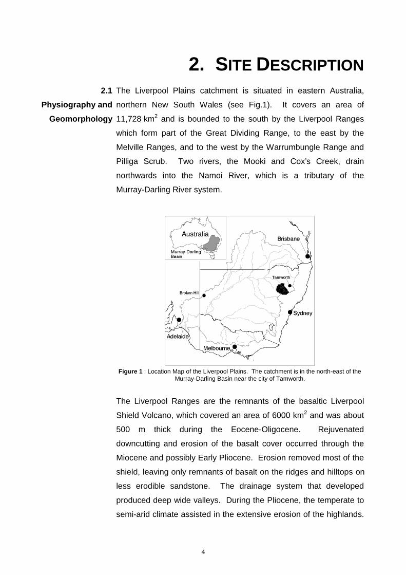
The Liverpool Plains catchment is situated in eastern Australia,

northern New South Wales (see Fig.1). It covers an area of

11,728 km2 and is bounded to the south by the Liverpool Ranges

which form part of the Great Dividing Range, to the east by the

Melville Ranges, and to the west by the Warrumbungle Range and

Pilliga Scrub. Two rivers, the Mooki and Cox’s Creek, drain

northwards into the Namoi River, which is a tributary of the

Murray-Darling River system.

Figure 1 : Location Map of the Liverpool Plains. The catchment is in the north-east of theMurray-Darling Basin near the city of Tamworth.

The Liverpool Ranges are the remnants of the basaltic Liverpool

Shield Volcano, which covered an area of 6000 km2 and was about

500 m thick during the Eocene-Oligocene. Rejuvenated

downcutting and erosion of the basalt cover occurred through the

Miocene and possibly Early Pliocene. Erosion removed most of the

shield, leaving only remnants of basalt on the ridges and hilltops on

less erodible sandstone. The drainage system that developed

produced deep wide valleys. During the Pliocene, the temperate to

semi-arid climate assisted in the extensive erosion of the highlands.

5

The first episode of sedimentation resulted in inter-bedded clays

with sand and gravel layers deposited by braided streams, called

the Gunnedah Formation. The Pleistocene witnessed a change

towards a drier climate. The reduction of rainfall produced smaller

river channels and resulted in a change from braided to meandering

streams which continue to the present. The sediment deposits on

the alluvial plains consist of dominantly brown clays, with laterally

discontinuous channel deposits resulting in shoe string sand lenses.

The latter depositional sequence is referred to as the Narrabri

Formation (Gates, 1980).

The black cracking clays formed on the surface of the Liverpool

Plains are a highly productive agricultural region. The catchment is

a National Dryland Salinity Program (NDSP) focus catchment and

concerns of dryland salinity in different areas have led to many

investigations, e.g. Bradd et al. (1994), Broughton (1994a, b),

Greiner (1994), Johnston et al. (1995), Debashish et al. (1996),

Greiner and Hall (1997), Timms (1998).

2.2

Hydrogeology

The bedrock basement is overlain by a layer of quaternary alluvium

described above, with a thickness up to 110 m. The lower part of

the alluvium, the Gunnedah Formation, contains gravels and sands,

while the upper part, the Narrabri Formation, contains mostly clays

and silts. These two formations are in partial hydraulic contact, with

the Narrabri formation acting as a semi-confining layer. Over the

lower half of the catchment, the Narrabri groundwater system is

saline with electrical conductivity values (EC) values up to

35 dS m-1, while the Gunnedah is uniformly fresh with EC <

2 dS m-1.

The underlying deep basement aquifers, consisting of tertiary

basalts, Triassic conglomerates, Permian basalts and limestone,

have saturated hydraulic conductivity values ranging between 10-4

and 1.0 m d-1 with EC values ranging from 1 to 2 dS m-1. According

to UNSW (Broughton 1994a) and CSIRO Land and Water (Andrew

6

Herczeg, pers. com., June 1997) water quality studies, there is only

minor mixing between the basement and alluvial aquifers. Bore

records also indicate deeply weathered fronts on the basement,

which reduces transmissivity (Gates, 1980). The most transmissive

groundwater system on the Liverpool Plains are the deeper alluvial

aquifers of the Gunnedah Formation.

2.3

Landuse

European settlement began in the 1830’s and the land was

predominantly used for sheep and cattle grazing. In the 1880’s

extensive tree clearing occurred as cropping became an important

land use on the lighter textured "red soils" on the footslopes. In the

early 1950’s, improved agricultural technology and practice allowed

the rich heavy clays of the low lying alluvial flats to become the main

agricultural area. Cropping on the footslopes was progressively

abandoned and replaced by grazed grasslands. Today the steep

ridges of the Ranges are covered by various species of eucalypts.

2.4

Climate

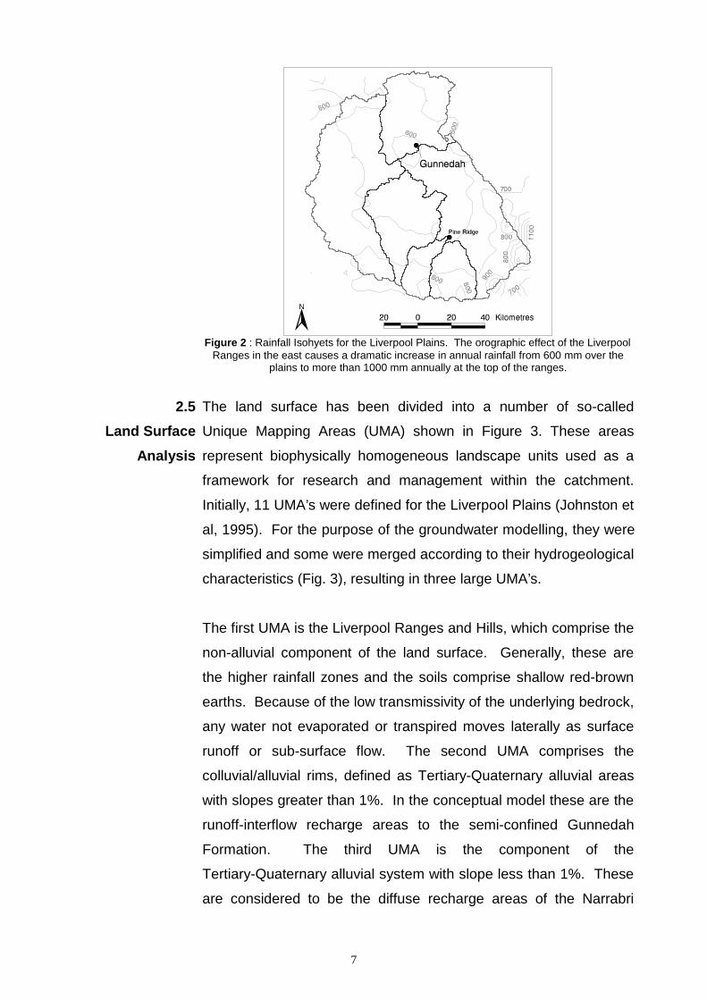
The annual rainfall decreases from over 1000mm at the top of the

Liverpool Ranges (elevation up to 1000m) in the south east to

600mm on the flats near Pine Ridge (elevation around 300m) (Fig.

2). Rain falls predominantly in the summer months, often in short

duration, high intensity rain or thunderstorms. Rainfall is extremely

variable between years and seasons, resulting in drought and low

river flows or flood conditions. Annual average potential

evaporation of the area is 1900mm, with a maximum monthly

average of 275mm in December and a minimum of 65mm in June.

7

Figure 2 : Rainfall Isohyets for the Liverpool Plains. The orographic effect of the LiverpoolRanges in the east causes a dramatic increase in annual rainfall from 600 mm over the

plains to more than 1000 mm annually at the top of the ranges.

2.5

Land Surface

Analysis

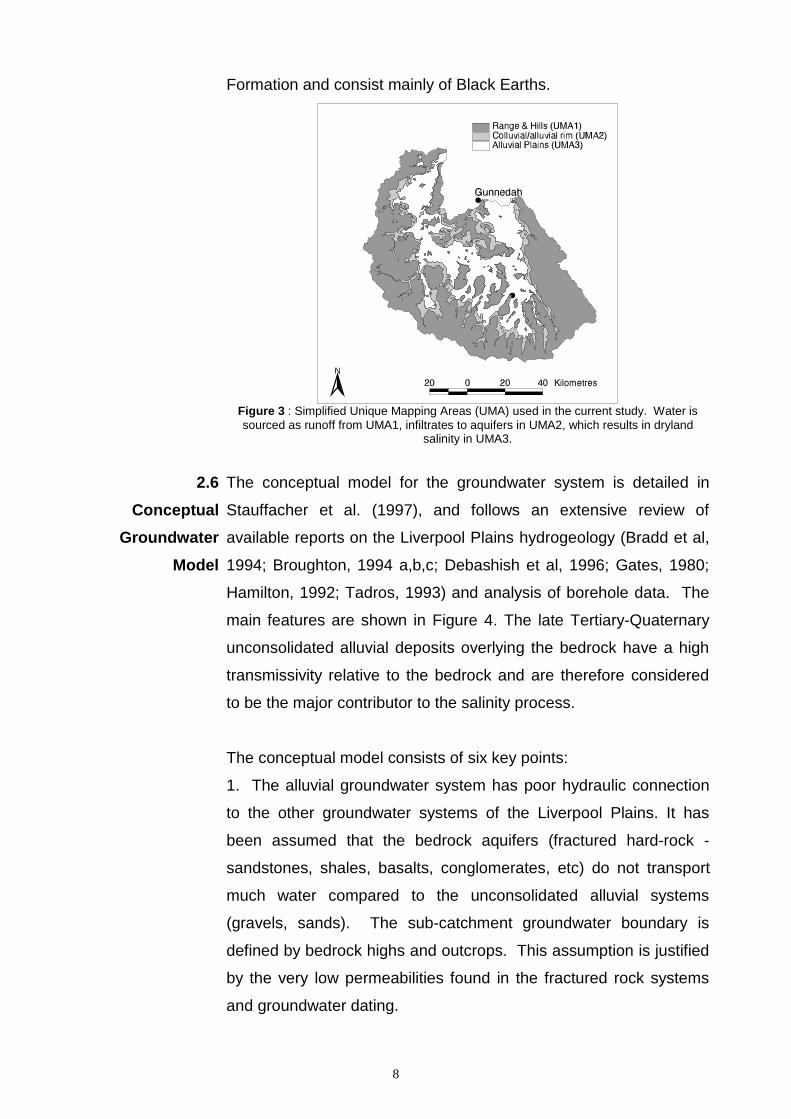
The land surface has been divided into a number of so-called

Unique Mapping Areas (UMA) shown in Figure 3. These areas

represent biophysically homogeneous landscape units used as a

framework for research and management within the catchment.

Initially, 11 UMA’s were defined for the Liverpool Plains (Johnston et

al, 1995). For the purpose of the groundwater modelling, they were

simplified and some were merged according to their hydrogeological

characteristics (Fig. 3), resulting in three large UMA’s.

The first UMA is the Liverpool Ranges and Hills, which comprise the

non-alluvial component of the land surface. Generally, these are

the higher rainfall zones and the soils comprise shallow red-brown

earths. Because of the low transmissivity of the underlying bedrock,

any water not evaporated or transpired moves laterally as surface

runoff or sub-surface flow. The second UMA comprises the

colluvial/alluvial rims, defined as Tertiary-Quaternary alluvial areas

with slopes greater than 1%. In the conceptual model these are the

runoff-interflow recharge areas to the semi-confined Gunnedah

Formation. The third UMA is the component of the

Tertiary-Quaternary alluvial system with slope less than 1%. These

are considered to be the diffuse recharge areas of the Narrabri

8

Formation and consist mainly of Black Earths.

Figure 3 : Simplified Unique Mapping Areas (UMA) used in the current study. Water issourced as runoff from UMA1, infiltrates to aquifers in UMA2, which results in dryland

salinity in UMA3.

2.6

Conceptual

Groundwater

Model

The conceptual model for the groundwater system is detailed in

Stauffacher et al. (1997), and follows an extensive review of

available reports on the Liverpool Plains hydrogeology (Bradd et al,

1994; Broughton, 1994 a,b,c; Debashish et al, 1996; Gates, 1980;

Hamilton, 1992; Tadros, 1993) and analysis of borehole data. The

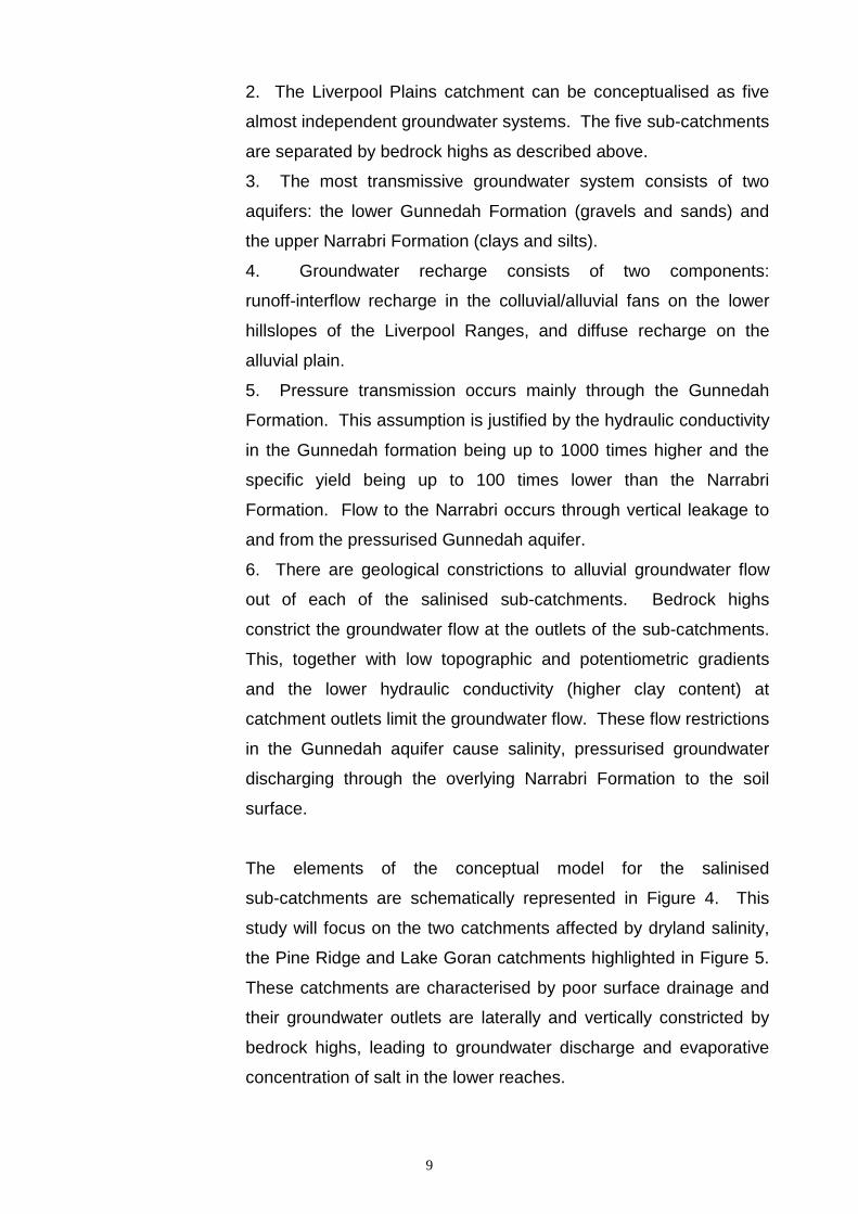
main features are shown in Figure 4. The late Tertiary-Quaternary

unconsolidated alluvial deposits overlying the bedrock have a high

transmissivity relative to the bedrock and are therefore considered

to be the major contributor to the salinity process.

The conceptual model consists of six key points:

1. The alluvial groundwater system has poor hydraulic connection

to the other groundwater systems of the Liverpool Plains. It has

been assumed that the bedrock aquifers (fractured hard-rock -

sandstones, shales, basalts, conglomerates, etc) do not transport

much water compared to the unconsolidated alluvial systems

(gravels, sands). The sub-catchment groundwater boundary is

defined by bedrock highs and outcrops. This assumption is justified

by the very low permeabilities found in the fractured rock systems

and groundwater dating.

9

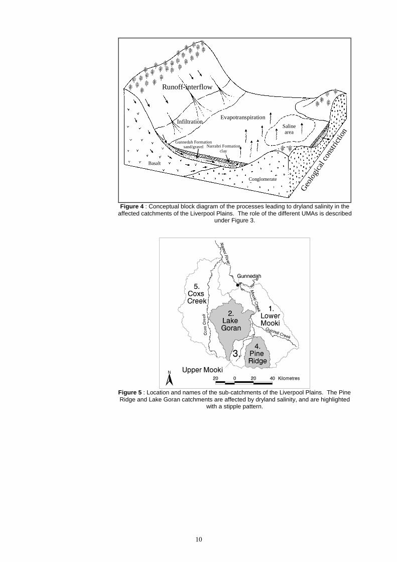
2. The Liverpool Plains catchment can be conceptualised as five

almost independent groundwater systems. The five sub-catchments

are separated by bedrock highs as described above.

3. The most transmissive groundwater system consists of two

aquifers: the lower Gunnedah Formation (gravels and sands) and

the upper Narrabri Formation (clays and silts).

4. Groundwater recharge consists of two components:

runoff-interflow recharge in the colluvial/alluvial fans on the lower

hillslopes of the Liverpool Ranges, and diffuse recharge on the

alluvial plain.

5. Pressure transmission occurs mainly through the Gunnedah

Formation. This assumption is justified by the hydraulic conductivity

in the Gunnedah formation being up to 1000 times higher and the

specific yield being up to 100 times lower than the Narrabri

Formation. Flow to the Narrabri occurs through vertical leakage to

and from the pressurised Gunnedah aquifer.

6. There are geological constrictions to alluvial groundwater flow

out of each of the salinised sub-catchments. Bedrock highs

constrict the groundwater flow at the outlets of the sub-catchments.

This, together with low topographic and potentiometric gradients

and the lower hydraulic conductivity (higher clay content) at

catchment outlets limit the groundwater flow. These flow restrictions

in the Gunnedah aquifer cause salinity, pressurised groundwater

discharging through the overlying Narrabri Formation to the soil

surface.

The elements of the conceptual model for the salinised

sub-catchments are schematically represented in Figure 4. This

study will focus on the two catchments affected by dryland salinity,

the Pine Ridge and Lake Goran catchments highlighted in Figure 5.

These catchments are characterised by poor surface drainage and

their groundwater outlets are laterally and vertically constricted by

bedrock highs, leading to groundwater discharge and evaporative

concentration of salt in the lower reaches.

10

Runoff-interflow

Salinearea

Gunnedah Formationsand/gravel

Geo

logi

cal c

onstr

ictio

n

Basalt

Narrabri Formationclay

Conglomerate

InfiltrationEvapotranspiration

Figure 4 : Conceptual block diagram of the processes leading to dryland salinity in theaffected catchments of the Liverpool Plains. The role of the different UMAs is described

under Figure 3.

Figure 5 : Location and names of the sub-catchments of the Liverpool Plains. The PineRidge and Lake Goran catchments are affected by dryland salinity, and are highlighted

with a stipple pattern.

11

3. AVAILABLE DATAThis section describes the available data and data processing

required to parameterise the FLOWTUBE groundwater model. The

sub-catchments used in this work are the three sub-catchments of

Pine Ridge, i.e. Big Jacks, Yarramanbah, and Pump Station Creeks,

and the Lake Goran catchment. As discussed in §2.5, these are the

catchments that exhibit dryland salinity associated with rising

groundwater tables, and groundwater flow constrictions.

3.1

Parameter

Estimation

Parameter values for a model can be obtained in a number of ways.

The most direct method is to measure parameters. However, the

time required to collect such parameter values for a large area can

be both expensive and time consuming. In many cases however,

the measurements are on the wrong areal scale (e.g. pump tests),

wrong time scale (e.g. water balance recharge measurements), or

are difficult to make (e.g. specific yield). So for this study,

groundwater parameters are inferred using six methods:

1. Correlating parameter values with more easily measured and

documented surrogates, e.g. conductivity estimated from measured

gravel, sand, silt, clay fractions;

2. Transferring values from hydrogeologically similar areas;

3. Calibrating the model against some related parameter, most

often groundwater levels, fluctuations and trends;

4. Comparison of model predictions of groundwater discharge into

streams or through evapotranspiration with those obtained from

stream salt loads or from area of saline land;

5. Comparison with results derived from hydrochemistry data, most

often carbon-14 (water travel time);

6. Comparison with values obtained at the wrong spatial or

temporal scale.

12

These methods are not independent and some overlap does occur.

Methods 1, 2, 4 and 6 usually define a possible range for a

groundwater parameter. For example using Method 1, the

conductivity of an unconsolidated gravel aquifer lies in the range of

10-3 m s-1 to 1 m s-1 (Freeze and Cherry, 1980) which is an extreme

range of values. The calibration processes in Methods 3 and 4

consist of fitting parameter values within the given range so that

model output best matches measured values. Without a predefined,

and preferably small, range to work within any calibration method

can be unreliable.

The more parameters that are varied during the calibration process,

the more easily measured values can be matched. However,

having confidence in the parameter values requires either having

only a few fitted parameters, or a degree of redundancy in the

dataset, i.e. the degrees of freedom in our dataset is greater than

the number of parameters that are varied. The more redundant

data that we have, the better we can estimate parameter

uncertainty. The amount of redundancy in a dataset is often difficult

to estimate because of the correlation in data, i.e. not all data may

be independent. For example, we may have 100 groundwater

bores, but they may not all act independently and effectively, there

may be only 6 independent bores. To reduce the number of

parameters varied during the calibration process, we often assume

the parameter values to be the same for regions of similar geology

(Method 2) and for the recharge to be spatially constant across any

one UMA. The calibration process does not provide an estimate of

systematic error, i.e. that error associated with an oversimplified

conceptual model. If, however, we can not match any measured

value, it is a sign of a wrong conceptual model.

3.2

Data Supporting

the Conceptual

Model

Some data analysis is performed when defining the conceptual

model of the system. These analyses provide the basis for the

conceptual model, and therefore define the range and applicability

of the numerical model. In the conceptual model we assume that

13

the catchments can be treated, modelled and managed separately

because they are hydrogeologically independent. The evidence for

this assumption lies in the structural role of the sandstone hills and

ridges intruding into the plains area. Bore hydrographs in these

features show water levels that are much deeper than bores drilled

into the Narrabri and Gunnedah Formations, and show distinctly

different responses where we have a reasonable time series. If the

sandstone is not hydraulically connected to the Gunnedah

Formation then intrusions through the surface should create

independent beds of Gunnedah Formation material that can be

treated separately.

The next important assumption is the role of evapotranspiration in

land salinisation. Hydrochemical analyses were performed on water

samples taken within the Yarramanbah Creek sub-catchment.

Samples were taken from bores along the length of the aquifer

transect used within the numerical modelling work and analysed for

various ions, cations and for 14C. The general conclusion from the

anion and cation analyses was that water from any of the three

layers was not significantly chemically different, except that the

water from the Narrabri Formation, the surface layer, had greater

total dissolved solids. This indicates that an evaporative process

has been occurring in this layer, which confirms the role of

evapotranspiration in salt build-up and dryland salinity stated in the

conceptual model.

Limited 14C results were used to delineate the role of the three

aquifer layers. A clear pattern of young water at the upper end of

the catchment and old water at the lower end of the catchment was

established. In the Gunnedah Formation, the age varied from "new"

water, to 5000 years old near the middle, to about 12000 years near

the outlet. In the basalt basement aquifer, the age starts at 4300

years old at the top, drops to 15500 year old near the middle, to

greater than 30000 years at the bottom. Two points emerge from

these data. Firstly that the assumption in the conceptual model that

14

the basement material plays no significant part in transport or

storage of water is justified. Secondly, these results support the

conceptual model of apparently one-dimensional flow, with the

Gunnedah Formation transmitting much of the water.

The area of surface discharge is important to both the conceptual

and numerical models. There are limited surface features indicating

salinisation in the Liverpool Plains, but there is the physical

evidence of high water table pressures in the Gunnedah Formation.

The area of surface discharge can be estimated from where these

heads are close to, or above, the soil surface. Where heads are

artesian, an estimate can be made of the maximum discharge rate,

but this was not required in the sub-catchments studied.

3.3

Structural Data

The FLOWTUBE groundwater model requires three types of input

data. The first is structural information that describes the physical

dimensions of the aquifers, according to the conceptual model

outlined in §2.6. Dyce and Richardson (1997) detail the lithological

logs available for the catchments of interest in the Liverpool Plains.

Additionally they show the cross-sections and long-sections used to

describe the shape and extent of the Narrabri and Gunnedah

Formations for each sub-catchment.

Each sub-catchment had between three and six cross-sections

derived from the sparse lithological log data where the three basic

layers were clearly identified. This identified the thickness of each

of the layers, providing vertical boundaries for the conducting

aquifer. Using topographic and geological maps, the width of the

aquifer was determined, under the assumptions in the conceptual

model on the bounding role of the sandstone hills. With the three

sub-catchments of the Pine Ridge catchment, each was described

as a single FLOWTUBE with no branches, consistent with the

conceptual model. In the case of the Lake Goran catchment, each

of the three north-south arms was described separately, then linked

to a central trunk section containing the lake itself.

15

3.4

Water Input Data

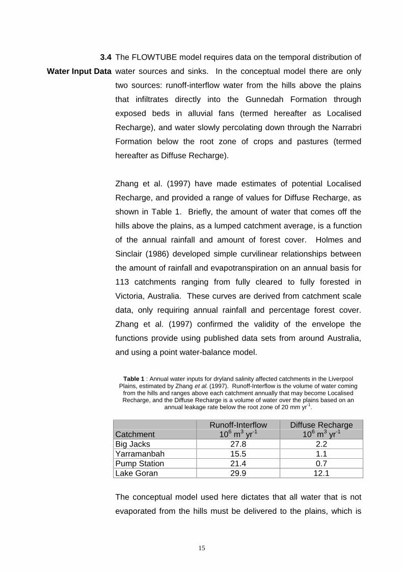
The FLOWTUBE model requires data on the temporal distribution of

water sources and sinks. In the conceptual model there are only

two sources: runoff-interflow water from the hills above the plains

that infiltrates directly into the Gunnedah Formation through

exposed beds in alluvial fans (termed hereafter as Localised

Recharge), and water slowly percolating down through the Narrabri

Formation below the root zone of crops and pastures (termed

hereafter as Diffuse Recharge).

Zhang et al. (1997) have made estimates of potential Localised

Recharge, and provided a range of values for Diffuse Recharge, as

shown in Table 1. Briefly, the amount of water that comes off the

hills above the plains, as a lumped catchment average, is a function

of the annual rainfall and amount of forest cover. Holmes and

Sinclair (1986) developed simple curvilinear relationships between

the amount of rainfall and evapotranspiration on an annual basis for

113 catchments ranging from fully cleared to fully forested in

Victoria, Australia. These curves are derived from catchment scale

data, only requiring annual rainfall and percentage forest cover.

Zhang et al. (1997) confirmed the validity of the envelope the

functions provide using published data sets from around Australia,

and using a point water-balance model.

Table 1 : Annual water inputs for dryland salinity affected catchments in the LiverpoolPlains, estimated by Zhang et al. (1997). Runoff-Interflow is the volume of water coming

from the hills and ranges above each catchment annually that may become LocalisedRecharge, and the Diffuse Recharge is a volume of water over the plains based on an

annual leakage rate below the root zone of 20 mm yr-1.

CatchmentRunoff-Interflow

106 m3 yr-1Diffuse Recharge

106 m3 yr-1

Big Jacks 27.8 2.2Yarramanbah 15.5 1.1Pump Station 21.4 0.7Lake Goran 29.9 12.1

The conceptual model used here dictates that all water that is not

evaporated from the hills must be delivered to the plains, which is

16

consistent with the Holmes-Sinclair model. Zhang et al. estimated

the amount of runoff-interflow water that potentially contributes to

Localised Recharge for three sub-catchments of the Liverpool

Plains, remembering the role of flooding in partitioning this water.

Two possible models are apparent for water that escapes the root

zone of plants on the plains. The first is that it slowly percolates

through the Narrabri Formation and recharges the Gunnedah

Formation. Given that the Gunnedah Formation is under pressure

however, indicates that it is confined and will not be receiving a

significant amount of water through this mechanism. The second

scenario is that high pressure forces the deep drainage to perch

locally in the shallow saline aquifer of the Narrabri Formation

causing storage changes in the surface soil only. This second

model is more likely and has implications for land-use management

of the discharge areas. Table 1 lists the values of runoff-interflow

and drainage below crop roots from Zhang et al. (1997). They

reported various estimates of drainage below crop roots, and a

representative value only is shown in Table 1 for comparison

purposes.

In the catchments within the Liverpool Plains flooding is a significant

process. In the Big Jacks Creek sub-catchment, a gauging station

was installed and has good records for 1996 to 1998. The data

from this three year period indicates that between 3 and 5% of the

rain falling in the hills and ranges leaves the catchment during

floods. The implication of this result is that there is a lot of water left

over which the conceptual model must take into account when

determining the water budget for Localised and Diffuse Recharge.

3.5

Physical State

Data

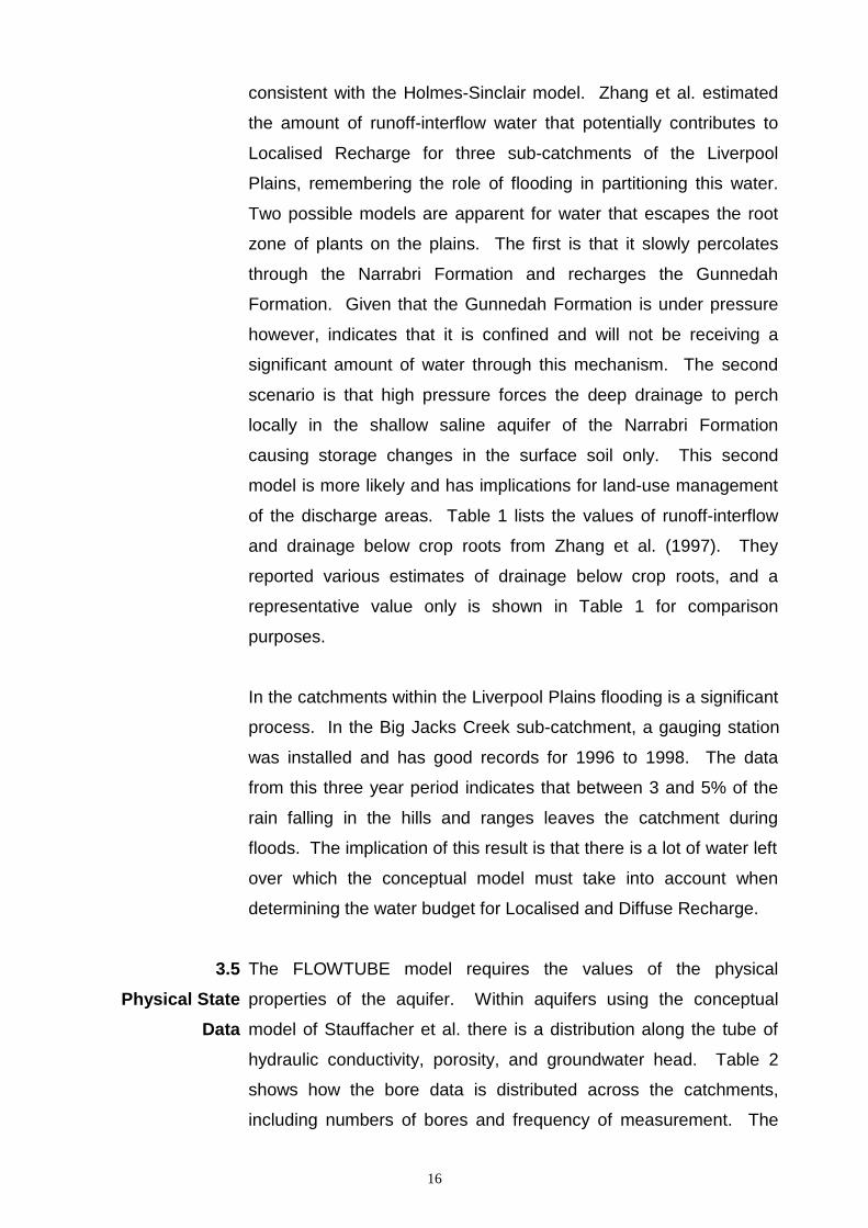
The FLOWTUBE model requires the values of the physical

properties of the aquifer. Within aquifers using the conceptual

model of Stauffacher et al. there is a distribution along the tube of

hydraulic conductivity, porosity, and groundwater head. Table 2

shows how the bore data is distributed across the catchments,

including numbers of bores and frequency of measurement. The

17

simple conclusion is that there is insufficient groundwater head data

to run simulations with transient inputs over any reasonable time

frame. For calibration purposes only long-term steady-state

simulations will be performed, by using constant input conditions

and running the model until calculated groundwater heads do not

change over a single year.

Table 2 : Available bore, lithology, hydrograph, and physical data for dryland salinityaffected catchments in the Liverpool Plains. The section for Long-term Hydrographs

indicates the number of piezometer nests and the length of time regular reading have beentaken for, and the Pump Test section indicates the number of pumping tests performed

along with the estimated hydraulic conductivity.

YarramanbahCreek

Big JacksCreek

Pump StationCreek

Lake GoranCatchment

Number ofBores

70 122 53 674

Valid Depthto Water

60 90 30 431

Lithology &>5 Readings

11 14 10 23

Long-termHydrograph

1, 8 years 1, 10 years 0 7, 24 years

Pump Testsand Results

0 1, 10-20m d-1

0 0

Hills/RangesArea, km2

102 213 118 354

ContactArea, km2

33 54 42 138

Plains Area,km2

55 110 35 605

Estimates of hydraulic conductivity and porosity are necessary to

the operation of the FLOWTUBE model, and several sources are

available for these values. The first of these parameters to be

assigned was porosity. On the basis of available data there was

little prospect of getting a distribution over any of the

sub-catchments, so it was assigned a constant value over all the

sub-catchments of 0.2. While there is feedback and compensation

between conductivity, porosity, and the rate of water level rise or

fall, there must be consistency between them also. Under the

steady-state conditions used in the initial modelling, and the fact that

the aquifers are primarily quite full and head controlled, porosity had

18

almost no effect on the outcomes. Further, in transient simulations

in §5 this value provides consistent rates of ground water rise.

The possible range of values for hydraulic conductivity is critical

however. Freeze and Cherry (1980) provide a table with the

expected range of values for hydraulic conductivity and porosity in

different materials, and suggests for gravel that conductivity is

between 10 and 1000 m d-1 and porosity is 0.05 to 0.2, and that for

clay porosity is 0.2 to 0.4. These ranges are too wide for use in a

model, and could yield any head distribution desired with

appropriate fitting.

The experience and expert knowledge of hydrogeologists working

as partners on this project is a useful source of data. They

suggested a range of 10 to 100 m d-1 for this and similar alluvial

systems in eastern Australia (W. R. Evans, pers. comm. 1997).

While it seems not to be rigorous to accept opinions and

experience, we must use all available sources to narrow down the

range of parameters when little real data exists, and acknowledge

that this type of data forms the basis of many modern expert

systems and decision support systems. We should place greater

error bounds on these data sources, however.

Salotti (1997) fitted both hydraulic conductivity and porosity to an

aquifer system in an adjacent catchment, named Borambil Creek.

There was 17 years worth of good quality bore hydrographs, with

irrigation and pumping data for the last ten years. The results of

fitting in MODFLOW (McDonald and Harbaugh, 1988) suggested a

range of conductivity from 1 to 30 m d -1 and a range of porosity of

0.05 to 0.3, for a single layer, combined sand and clay aquifer, of

similar dimensions to those in Pine Ridge. Given that the modelled

aquifer contained gravel, sand, and clay, the cleaner aquifer

systems modelled in the Liverpool Plains catchments would have a

higher conductivity than fitted by Salotti.

19

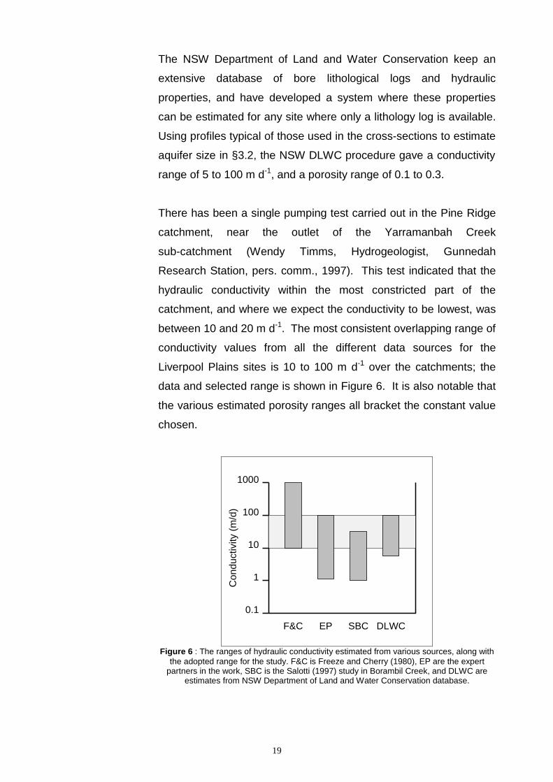
The NSW Department of Land and Water Conservation keep an

extensive database of bore lithological logs and hydraulic

properties, and have developed a system where these properties

can be estimated for any site where only a lithology log is available.

Using profiles typical of those used in the cross-sections to estimate

aquifer size in §3.2, the NSW DLWC procedure gave a conductivity

range of 5 to 100 m d-1, and a porosity range of 0.1 to 0.3.

There has been a single pumping test carried out in the Pine Ridge

catchment, near the outlet of the Yarramanbah Creek

sub-catchment (Wendy Timms, Hydrogeologist, Gunnedah

Research Station, pers. comm., 1997). This test indicated that the

hydraulic conductivity within the most constricted part of the

catchment, and where we expect the conductivity to be lowest, was

between 10 and 20 m d-1. The most consistent overlapping range of

conductivity values from all the different data sources for the

Liverpool Plains sites is 10 to 100 m d-1 over the catchments; the

data and selected range is shown in Figure 6. It is also notable that

the various estimated porosity ranges all bracket the constant value

chosen.

DLWCSBCEPF&C

0.1

1

10

100

1000

Con

duct

ivity

(m

/d)

Figure 6 : The ranges of hydraulic conductivity estimated from various sources, along withthe adopted range for the study. F&C is Freeze and Cherry (1980), EP are the expert

partners in the work, SBC is the Salotti (1997) study in Borambil Creek, and DLWC areestimates from NSW Department of Land and Water Conservation database.

20

4. NUMERICAL MODELThe FLOWTUBE groundwater model was developed to be as

simple as possible, requiring the fewest number of parameters and

least amount of input data, yet incorporate all the key processes of

groundwater movement in alluvial systems. The basis of the

method is to develop a groundwater budget of the catchment. The

catchment is first described as a segmented tube and a

groundwater balance is calculated for each cell. Inflows to each cell

are vertical recharge over the cell, and lateral movement of water

from higher up in the catchment. Outflows from each cell are

surface discharge out of the cell, and lateral movement of

groundwater to parts lower down in the catchment. The difference

between inputs and output will cause a rising or lowering of the

groundwater. All lateral fluxes are calculated using Darcy’s Law.

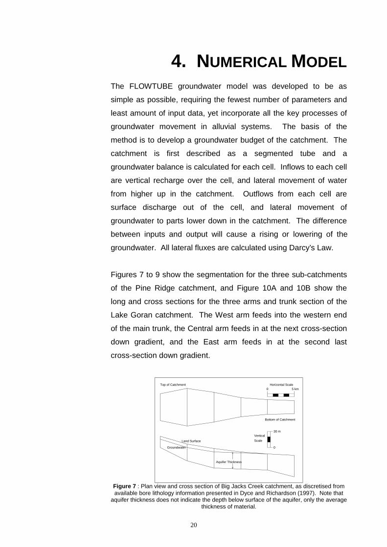
Figures 7 to 9 show the segmentation for the three sub-catchments

of the Pine Ridge catchment, and Figure 10A and 10B show the

long and cross sections for the three arms and trunk section of the

Lake Goran catchment. The West arm feeds into the western end

of the main trunk, the Central arm feeds in at the next cross-section

down gradient, and the East arm feeds in at the second last

cross-section down gradient.

Land Surface

Groundwater

Aquifer Thickness

0 5 km

0

30 m

Horizontal Scale

Vertical

Scale

Top of Catchment

Bottom of Catchment

Figure 7 : Plan view and cross section of Big Jacks Creek catchment, as discretised fromavailable bore lithology information presented in Dyce and Richardson (1997). Note that

aquifer thickness does not indicate the depth below surface of the aquifer, only the averagethickness of material.

21

Top of Catchment

Land Surface

Groundwater

Aquifer Thickness

0 5 km

30 m

0

Horizontal Scale

Scale

Vertical

Bottom of Catchment

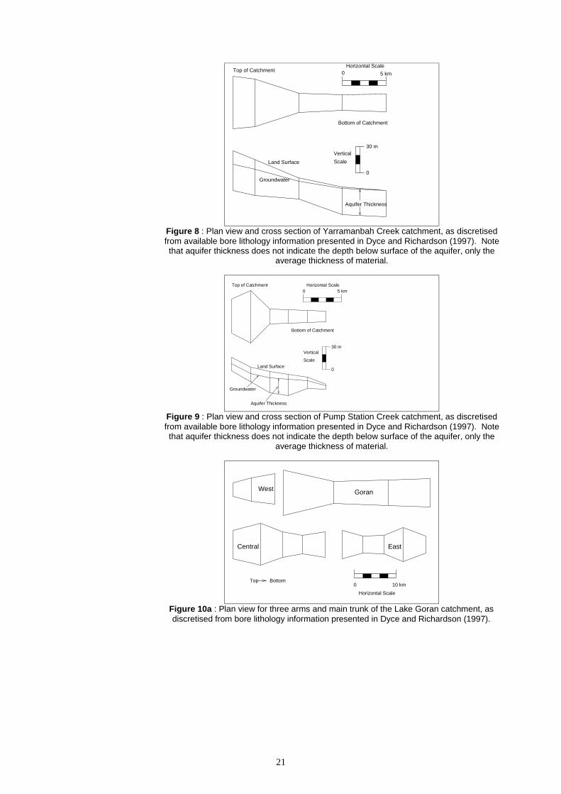
Figure 8 : Plan view and cross section of Yarramanbah Creek catchment, as discretisedfrom available bore lithology information presented in Dyce and Richardson (1997). Notethat aquifer thickness does not indicate the depth below surface of the aquifer, only the

average thickness of material.

Top of Catchment

Land Surface

Groundwater

Aquifer Thickness

Bottom of Catchment

0 5 kmHorizontal Scale

0

30 mVertical

Scale

Figure 9 : Plan view and cross section of Pump Station Creek catchment, as discretisedfrom available bore lithology information presented in Dyce and Richardson (1997). Notethat aquifer thickness does not indicate the depth below surface of the aquifer, only the

average thickness of material.

GoranWest

Central East

0 10 km

Horizontal Scale

Top Bottom

Figure 10a : Plan view for three arms and main trunk of the Lake Goran catchment, asdiscretised from bore lithology information presented in Dyce and Richardson (1997).

22

EasternCentral

West Goran

Land Surface

Groundwater

Aquifer Thickness

0

50 mVertical

Scale

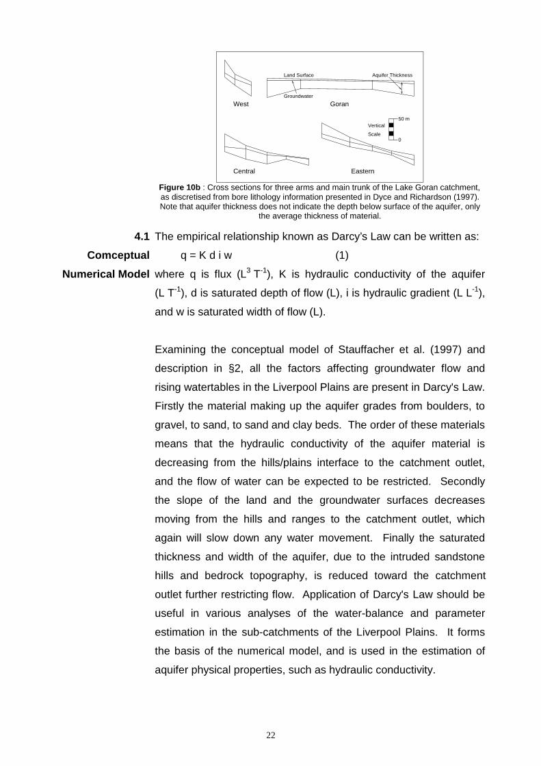
Figure 10b : Cross sections for three arms and main trunk of the Lake Goran catchment,as discretised from bore lithology information presented in Dyce and Richardson (1997).Note that aquifer thickness does not indicate the depth below surface of the aquifer, only

the average thickness of material.

4.1

Comceptual

Numerical Model

The empirical relationship known as Darcy’s Law can be written as:

q = K d i w (1)

where q is flux (L3 T-1), K is hydraulic conductivity of the aquifer

(L T-1), d is saturated depth of flow (L), i is hydraulic gradient (L L-1),

and w is saturated width of flow (L).

Examining the conceptual model of Stauffacher et al. (1997) and

description in §2, all the factors affecting groundwater flow and

rising watertables in the Liverpool Plains are present in Darcy's Law.

Firstly the material making up the aquifer grades from boulders, to

gravel, to sand, to sand and clay beds. The order of these materials

means that the hydraulic conductivity of the aquifer material is

decreasing from the hills/plains interface to the catchment outlet,

and the flow of water can be expected to be restricted. Secondly

the slope of the land and the groundwater surfaces decreases

moving from the hills and ranges to the catchment outlet, which

again will slow down any water movement. Finally the saturated

thickness and width of the aquifer, due to the intruded sandstone

hills and bedrock topography, is reduced toward the catchment

outlet further restricting flow. Application of Darcy's Law should be

useful in various analyses of the water-balance and parameter

estimation in the sub-catchments of the Liverpool Plains. It forms

the basis of the numerical model, and is used in the estimation of

aquifer physical properties, such as hydraulic conductivity.

23

4.2 Numerical

Implementation

The FLOWTUBE groundwater model is a solution of 1-D Darcy’s

Law for saturated flow, with variable properties along a tube. There

are special conditions however for the conceptual model we are

using that affect the equations. Reiterating, they are:

1. The groundwater system consists of three layers (the

semi-confining Narrabri Formation the highly conductive Gunnedah

formation, and some bedrock material).

2. Underlying the region of interest is some basement material

which plays no role in groundwater movement or storage (in effect

this simply provides a lower limit to the extent of the aquifer).

3. The middle layer is a highly conductive aquifer, and the water in

this layer is assumed to always be under pressure, ie. the heads are

above the top of the aquifer, and so this layer contributes to water

movement only.

4. At the surface is a semi-confining layer with low conductivity; this

layer contributes to storage of water under pressure but not to any

lateral movement of water.

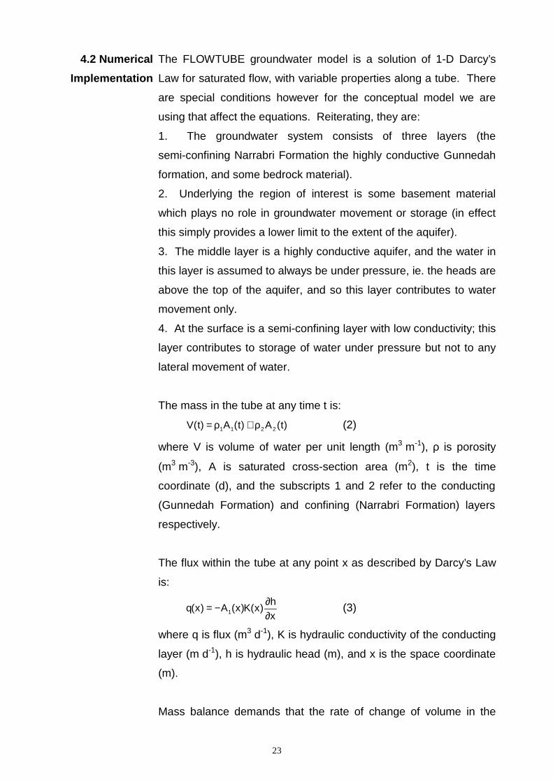
The mass in the tube at any time t is:

)t(A)t(A)t(V 2211 ρ+ρ= (2)

where V is volume of water per unit length (m3 m-1), ρ is porosity

(m3 m-3), A is saturated cross-section area (m2), t is the time

coordinate (d), and the subscripts 1 and 2 refer to the conducting

(Gunnedah Formation) and confining (Narrabri Formation) layers

respectively.

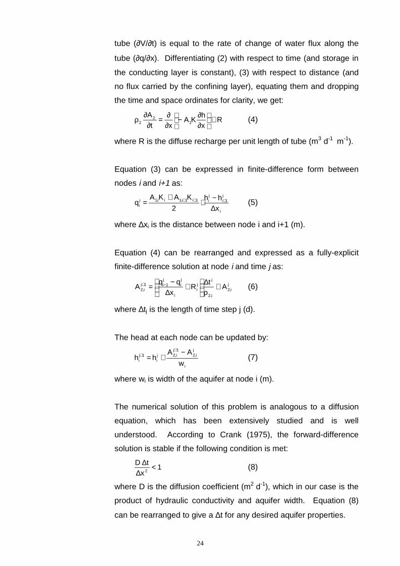
The flux within the tube at any point x as described by Darcy’s Law

is:

xh

)x(K)x(A)x(q 1 ∂∂−= (3)

where q is flux (m3 d-1), K is hydraulic conductivity of the conducting

layer (m d-1), h is hydraulic head (m), and x is the space coordinate

(m).

Mass balance demands that the rate of change of volume in the

24

tube (∂V/∂t) is equal to the rate of change of water flux along the

tube (∂q/∂x). Differentiating (2) with respect to time (and storage in

the conducting layer is constant), (3) with respect to distance (and

no flux carried by the confining layer), equating them and dropping

the time and space ordinates for clarity, we get:

Rxh

KAxt

A1

22 +

∂∂−

∂∂=

∂∂ρ (4)

where R is the diffuse recharge per unit length of tube (m3 d-1 m-1).

Equation (3) can be expressed in finite-difference form between

nodes i and i+1 as:

i

j1i

ji1i1i,1ii,1j

i xhh

2

KAKAq

∆−⋅

+= +++ (5)

where ∆xi is the distance between node i and i+1 (m).

Equation (4) can be rearranged and expressed as a fully-explicit

finite-difference solution at node i and time j as:

ji,2

i,2

jji

i

ji

j1i1j

i,2 At

Rx

qqA +

ρ∆

+

∆−

= −+ (6)

where ∆tj is the length of time step j (d).

The head at each node can be updated by:

i

ji,2

1ji,2j

i1j

i w

AAhh

−+=

++ (7)

where wi is width of the aquifer at node i (m).

The numerical solution of this problem is analogous to a diffusion

equation, which has been extensively studied and is well

understood. According to Crank (1975), the forward-difference

solution is stable if the following condition is met:

1x

tD2

<∆

∆ (8)

where D is the diffusion coefficient (m2 d-1), which in our case is the

product of hydraulic conductivity and aquifer width. Equation (8)

can be rearranged to give a ∆t for any desired aquifer properties.

25

4.3

Additional Model

Features

This model has been implemented with a tree structure of tubes,

requiring only trivial modifications to the conceptual and numerical

model. This allows for more complex aquifer geometry, assuming

the tube only has one main trunk and does not split as water moves

downstream.

Surface discharge with high groundwater pressures has been

implemented. A maximum discharge rate is specified and if

groundwater pressures cause the head to go above the surface

then one of two conditions results. Either all the excess water is

discharged and the groundwater head is at the land surface, or the

maximum allowable amount of water is discharged and the extra

contributes to groundwater heads that are above the ground surface

level. The maximum discharge rate can be zero for completely

confined systems.

The FLOWTUBE model also allows arbitrary spatial and temporal

distributions of recharge or groundwater loss, but does not allow

point sinks such as pumping wells. Negative recharge rates can be

specified, but local conditions will control drawdown and sustainable

pumping rates from actual wells.

26

5. MODEL CALIBRATIONIn §3 it was established that there is some information available on

all of the parameters required to run the FLOWTUBE model. These

are the physical shape and extent of the aquifer and confining layer,

the physical properties of the aquifer, the current water levels, and

the Localised and Diffuse Recharge components. Given that (1) the

size and shape of the aquifer is measured and fixed, (2) that the

current water levels are measured and representative, and (3) that

porosity and Diffuse Recharge are of secondary importance and can

be held constant, the parameters that require fitting are the

hydraulic conductivity of the aquifer, within the range defined in

§3.5, and the proportion of runoff-interflow that becomes Localised

Recharge to the aquifer. These parameters are co-dependent and

the combination must fit within all the constraints implicit in the

observed data.

It is desirable for both pragmatic and physical reasons to have the

proportion of runoff that becomes Localised Recharge constant for

each of the three sub-catchments of the Pine Ridge catchment.

This is because we would expect the erosion history of each of

these to be similar, and therefore the processes and rates of flows

to be similar. While this condition does not necessarily apply to the

Lake Goran catchment, for the purpose of this calibration exercise

the proportion of runoff that becomes Localised Recharge found in

the Pine Ridge catchments will be applied to Lake Goran.

5.1

Factors Affecting

Localised

Recharge

The FLOWTUBE model is a combination of Darcys' Law and a

mass balance equation. It is possible to rearrange (1) from §4.1 to

establish a relationship between the amount of Localised Recharge

and the hydraulic conductivity at the hills/plains interface, thus:

widRO

fK = (9)

where RO is the average rate of runoff from the hills and ranges

27

(m3 d-1), and f is the proportion of that runoff that becomes Localised

Recharge. The amount of Localised Recharge must satisfy several

constraints. First it should be an amount that when taken on an

annual average basis, does not require an absurdly large value of

deep drainage to infiltrate through the alluvial fans of the

catchments. Second given that there is not widespread water level

rise across these catchments, it must be in some equilibrium with

the groundwater flow at the catchment outlet. Third it must produce

a conductivity estimate from (9) in the recharge area at the top of

the catchment that is consistent with the a priori range determined in

§3, ie. between 10 and 100 m d-1. On the basis of these limiting

factors, we propose that 5% of the runoff-interflow from the hills

becomes Localised Recharge in each sub-catchment.

Using the area of alluvial fans in Table 2 and the volumes of

Runoff-Interflow water from Table 1, an estimate of the annual

average recharge rate in the alluvial fans can be made. In the

sub-catchments of the Pine Ridge catchment, the average rate

varies between 0.06 and 0.07 mm d-1, and in the Lake Goran

catchment the average rate is 0.05 mm d-1. This is an important

result, and is a reality check. If the infiltration rates required were

too high then the recharge process suggested in the conceptual

model would not be credible. Since they are low it suggests

available storage and not available water is the mechanism limiting

recharge. Another result to come from these calculations is that the

average rate for each of the three sub-catchments in Pine Ridge are

almost the same. This is good evidence that these sub-catchments

evolved together, and have similar hydrogeological behaviour. The

fact that the rate is also very similar in the Lake Goran catchment,

with different annual rainfall amounts, adds weight to the

assumption of a fixed proportion of runoff-interflow water becoming

Localised Recharge.

28

5.2

Steady-state

Calibration

With a fixed aquifer geometry and any given amount of Localised

Recharge, we can calculate what the conductivity will be with any

distribution of hydraulic heads using (9). An inferred conductivity

distribution that is relatively constant, or that is monotonically

increasing or decreasing along the tube, will provide further

confidence in the physical structure and conceptual model. If the

distribution is random or chaotic however, then without significant

geological changes along the tube this would indicate a poorly

constructed model. Additional to calculating conductivity within the

flow tube, using the results of the pump test at the catchment outlet

from Table 2, we can infer the hydraulic gradient at the outlet and fix

this as a boundary condition for the model.

In Big Jacks Creek a small area 5 km from the outlet showed high

conductivity estimates outside the prescribed range. It is a simple

conclusion that this area is likely to suffer from rising water levels

with increased water inputs. In the model runs, this area was

allowed to have the maximum hydraulic conductivity in the range

only (100 m d-1), and showed the greatest rates of rise with transient

simulations. Yarramanbah Creek had well behaved conductivity

estimates throughout except right at the outlet where salinity is

expected to be expressed. Pump Station Creek required a high

conductivity across the entire catchment due to its very thin lower

section. This also inferred a high hydraulic gradient at the outlet of

1%. A similar large drop in water level was reported by Timms

(1998) who measured groundwater depth along transects passing

through the outlet of the Pine Ridge Catchment, so this model

inference can be accepted as real. In the Lake Goran Catchment,

conductivity estimates were uniformly low, near the bottom of the

range, except in the main trunk. Here a significant area required

much higher conductivity to transmit the input water. Since this area

contains the lake this was not seen as unusual, but conductivity was

lowered to be consistent with the other fitted values; water levels

here were modelled at the ground surface.

29

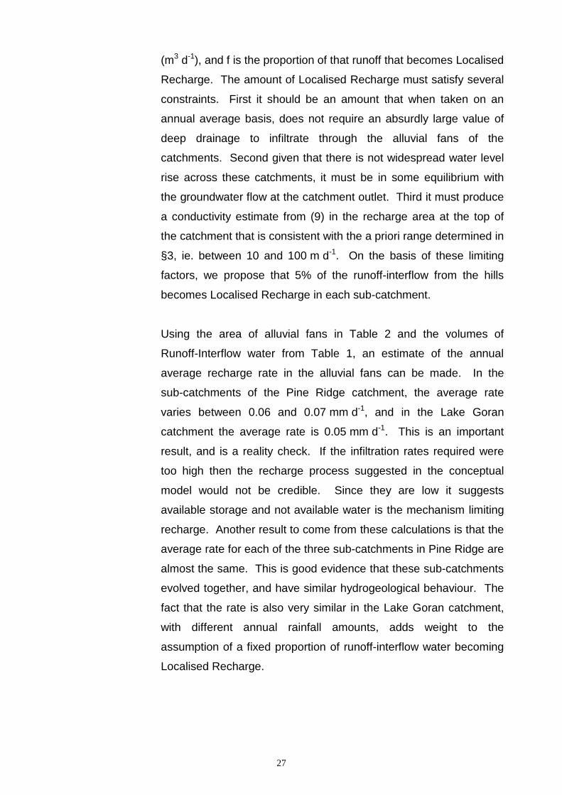
Conductivity estimates were rounded to multiples of 5 and some

manual modifications performed to allow for this rounding. Figures

11 to 14 show the fitted steady-state hydraulic heads for Big Jacks

Creek, Yarramanbah Creek, Pump Station Creek and Lake Goran,

respectively. The fits are excellent, as would be expected from

calculating conductivity based on the heads to be fitted. All the

catchments showed conductivity distributions that were well

behaved, and thus we can be more confident in the structure of the

aquifers and the conceptual model.

310

320

330

340

350

360

0 5 10 15 20 25

Distance (km)

Ele

vati

on

(m

AH

D)

GroundwaterSurface ElevationFitted Heads

Figure 11 : Measured and fitted steady-state groundwater heads in the GunnedahFormation for Big Jacks Creek catchment. The root mean square error (RMSE) between

the observed and calculated heads is 0.69 m.

300

310

320

330

340

350

360

0 3 6 9 12 15 18

Distance(km)

Ele

vati

on

(m

AH

D)

GroundwaterSurface ElevationFitted Heads

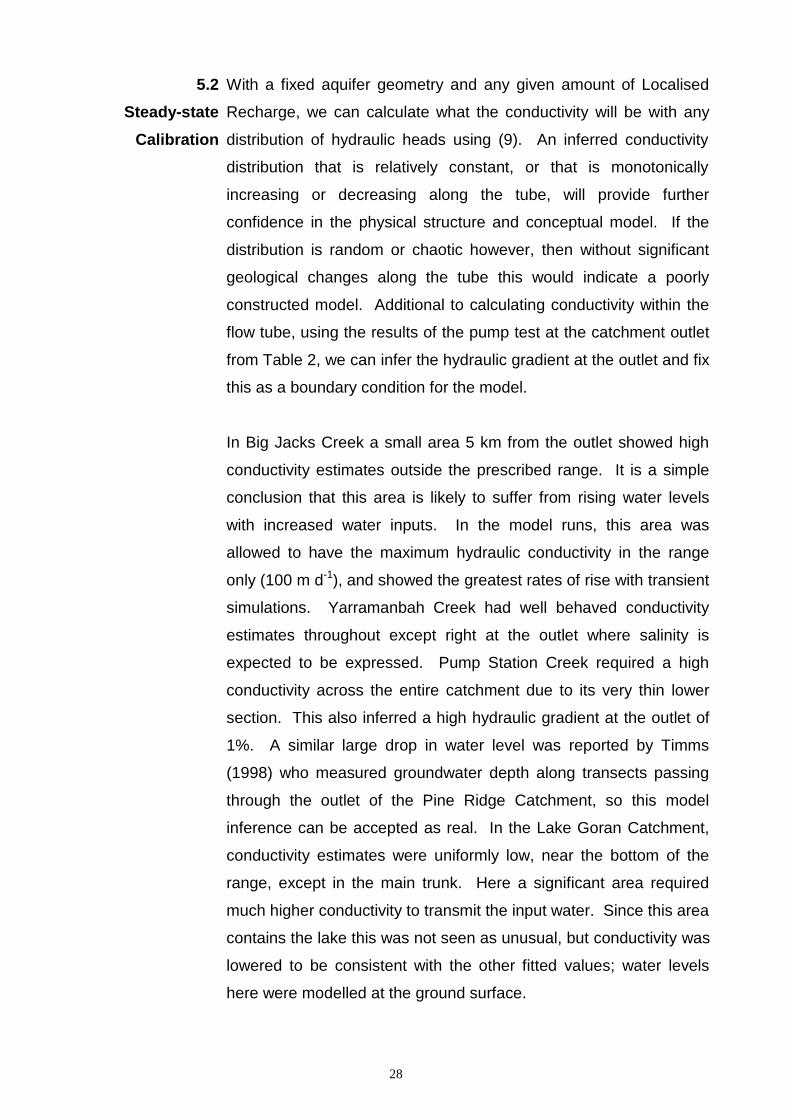
Figure 12 : Measured and fitted steady-state groundwater heads in the GunnedahFormation for Yarramanbah Creek catchment. The RMSE between the observed and

calculated heads is 0.70 m.

30

310

320

330

340

350

360

0.0 2.5 5.0 7.5 10.0 12.5

Distance (km)

Ele

vati

on

(m

AH

D)

GroundwaterSurface ElevationFitted Heads

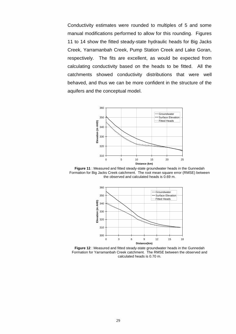
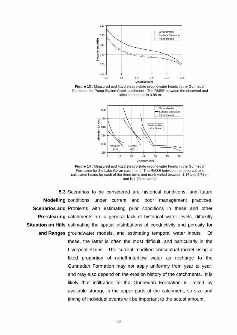
Figure 13 : Measured and fitted steady-state groundwater heads in the GunnedahFormation for Pump Station Creek catchment. The RMSE between the observed and

calculated heads is 0.85 m.

280

300

320

340

360

380

0 15 30 45 60 75 90

Distance (km)

Ele

vati

on

(m

AH

D)

GroundwaterSurface ElevationFitted Heads

WesternArm

CentralArm

Eastern Arm,Lake Goran

Figure 14 : Measured and fitted steady-state groundwater heads in the GunnedahFormation for the Lake Goran catchment. The RMSE between the observed and

calculated heads for each of the three arms and trunk varied between 1.17 and 2.71 m,and is 1.78 m overall.

5.3

Modelling

Scenarios and

Pre-clearing

Situation on Hills

and Ranges

Scenarios to be considered are historical conditions, and future

conditions under current and poor management practices.

Problems with estimating prior conditions in these and other

catchments are a general lack of historical water levels, difficulty

estimating the spatial distributions of conductivity and porosity for

groundwater models, and estimating temporal water inputs. Of

these, the latter is often the most difficult, and particularly in the

Liverpool Plains. The current modified conceptual model using a

fixed proportion of runoff-interflow water as recharge to the

Gunnedah Formation may not apply uniformly from year to year,

and may also depend on the erosion history of the catchments. It is

likely that infiltration to the Gunnedah Formation is limited by

available storage in the upper parts of the catchment, so size and

timing of individual events will be important to the actual amount.

31

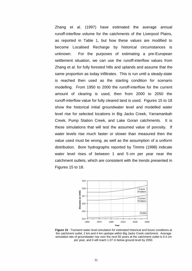
Zhang et al. (1997) have estimated the average annual

runoff-interflow volume for the catchments of the Liverpool Plains,

as reported in Table 1, but how these values are modified to

become Localised Recharge by historical circumstances is

unknown. For the purposes of estimating a pre-European

settlement situation, we can use the runoff-interflow values from

Zhang et al. for fully forested hills and uplands and assume that the

same proportion as today infiltrates. This is run until a steady-state

is reached then used as the starting condition for scenario

modelling. From 1950 to 2000 the runoff-interflow for the current

amount of clearing is used, then from 2000 to 2050 the

runoff-interflow value for fully cleared land is used. Figures 15 to 18

show the historical initial groundwater level and modelled water

level rise for selected locations in Big Jacks Creek, Yarramanbah

Creek, Pump Station Creek, and Lake Goran catchments. It is

these simulations that will test the assumed value of porosity. If

water levels rise much faster or slower than measured then the

value used must be wrong, as well as the assumption of a uniform

distribution. Bore hydrographs reported by Timms (1998) indicate

water level rises of between 1 and 5 cm per year near the

catchment outlets, which are consistent with the trends presented in

Figures 15 to 18.

314

315

316

317

318

319

1950 1970 1990 2010 2030 2050

Year

Ele

vati

on

(m

AH

D)

Outlet

CurrentProblem

FutureProblem

Figure 15 : Transient water level simulation for estimated historical and future conditions atthe catchment outlet, 2 km and 4 km upslope within Big Jacks Creek catchment. Averagesimulated rate of groundwater rise over the next 50 years at the catchment outlet is 0.4 cm

per year, and it will reach 1.07 m below ground level by 2050.

32

308

309

310

311

312

313

1950 1970 1990 2010 2030 2050

Year

Ele

vati

on

(m

AH

D)

Outlet

FutureProblems

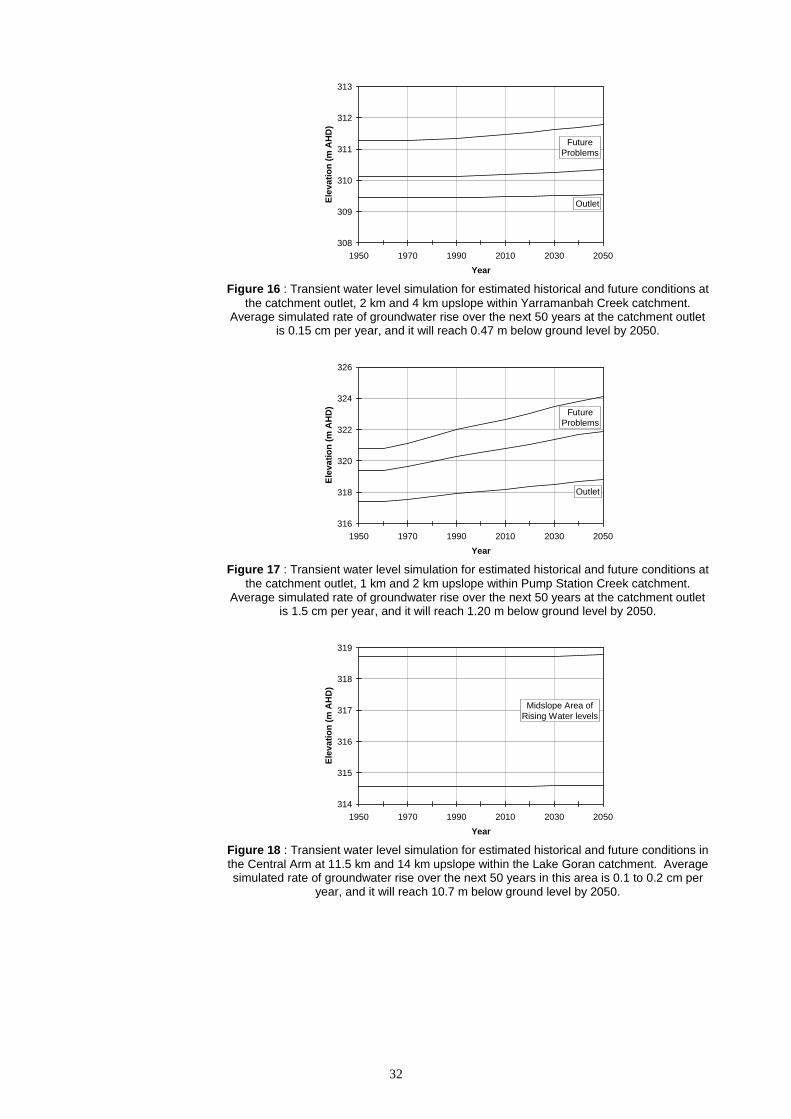
Figure 16 : Transient water level simulation for estimated historical and future conditions atthe catchment outlet, 2 km and 4 km upslope within Yarramanbah Creek catchment.

Average simulated rate of groundwater rise over the next 50 years at the catchment outletis 0.15 cm per year, and it will reach 0.47 m below ground level by 2050.

316

318

320

322

324

326

1950 1970 1990 2010 2030 2050

Year

Ele

vati

on

(m

AH

D)

Outlet

FutureProblems

Figure 17 : Transient water level simulation for estimated historical and future conditions atthe catchment outlet, 1 km and 2 km upslope within Pump Station Creek catchment.

Average simulated rate of groundwater rise over the next 50 years at the catchment outletis 1.5 cm per year, and it will reach 1.20 m below ground level by 2050.

314

315

316

317

318

319

1950 1970 1990 2010 2030 2050

Year

Ele

vati

on

(m

AH

D)

Midslope Area ofRising Water levels

Figure 18 : Transient water level simulation for estimated historical and future conditions inthe Central Arm at 11.5 km and 14 km upslope within the Lake Goran catchment. Averagesimulated rate of groundwater rise over the next 50 years in this area is 0.1 to 0.2 cm per

year, and it will reach 10.7 m below ground level by 2050.

33

6. DISCUSSION6.1

Impossible Values

of Hydraulic

Conductivity

It is common for measurements and estimates of hydraulic

conductivity to cover a single order or magnitude or more in both

surface soils and groundwater aquifer materials (eg. Freeze and

Cherry 1980, Timms 1998). In the present case we have estimated

from a variety of sources that hydraulic conductivity lies in the order

of 10 to 100 m d-1. If the order of magnitude was 100 to 1000 m d-1

or 1000 to 10000 m d-1, what are the site implications?

We calculate that 100% of the runoff-interflow water could be

transmitted through the current aquifer geometry of each of the

sub-catchments if the hydraulic conductivity was between 1000 and

5000 m d-1. If this was the case either there would be no floods,

which in fact are occurring more often (Dryland Salinity

Management Working Group 1993), or the watertables would be

below the surface and not rising. Since neither of these are

happening, the conductivity must be less than 1000 m d-1.

If the values of hydraulic conductivity were less than 1 m d-1, then

either all the watertables would be at the surface causing surface

salinisation throughout the plains, surface discharge would be at an

unrealistically high rate, a lake or permanent stream would develop,

or much more runoff-interflow would be gauged in streams following

flood events. We know that the watertables are not uniformly high,

there is not surface salinisation over the entire plains, and there are

not permanent water features in the sub-catchments with dryland

salinity. Therefore the conductivity must be greater than 1 m d-1.

The combined evidence of overlapping ranges of different

conductivity estimates, plus the co-dependence of conductivity and

Localised Recharge, along with the reality of the site situation,

strongly support the conductivity range used.

34

6.2

The Rest of the

Waterbalance

What of the rest of the water from the runoff-interflow balance? We

have reasonably asserted that a proportion of 5% enters the

groundwater system, and measured about 5% leaving during flood

events, so where does the other 90% go? The only possible sinks

are the basement material underlying the Gunnedah Formation, and

the storage and evaporation of flood water as it sits on the surface

of the plains. While water does appear in the bedrock, 14C results

indicate that this is very slow moving and is probably not a

significant sink in the system.

This leaves storage on the plains as the only candidate to close the

runoff-interflow budget. The weather systems in the Liverpool

Plains consist of steady frontal rain in the winter months, and more

violent convective thunder storms in the summer months. Zhang et

al. (1997) and Ringrose-Voase (pers. comm., 1999) have provided

estimates of the amount of available storage in the cracking clays of

the Liverpool Plains. In the top 2 m of soil up to 400 mm of storage

is available. Anecdotal evidence suggests that the clay plains

initially absorb large runoff events, but if followed closely by a

second large event, flooding occurs on the saturated plains. If the

heavy summer rains cause most flooding events, then it is possible

to evaporate a large amount of surface water when the potential

evaporation rates are highest to empty this store ready for the next

event. The depth to which plants can empty the soil store will

therefore contribute to more or less flood events, so the practice of

removing deep-rooted perennials for shallow-rooted crops may be a

factor contributing to increased flooding.

6.3

Scenario Results

The results of equilibrium simulations, historical scenario runs and

the conceptual model, provide much source for discussion. Firstly,

the measured and modelled water level fluctuations suggest that the

Gunnedah Formation is essentially full, with only a slow rise in water

pressure. The role of this high water level in relation to the shallow

saline aquifer in the Narrabri Formation has important management

35

implications. We suspect that the pressure in the Gunnedah

Formation prevents deep percolation below the shallow root zone of

many crops and grasses. Any water that escapes the reach of

vegetation will therefore contribute to a rise in the local perched

aquifer, which leads to localised salinity through evaporative

concentration. A secondary result is that the available storage in

the soil is reduced, and therefore the plains capacity to absorb large

rainfall events is reduced, making floods more frequent or severe,

and other land degradation problems associated with saturated soil

and increased runoff. Given that water levels are high already, even

the most careful management may only be buying time, and not

reversing any salinity or water level trends.

Thus far the Gunnedah Formation has been modelled as receiving

zero recharge through the Narrabri Formation. Poor management

can result in a local impact given that current agricultural systems

are leaking water. Under this regime, no management practice on

the plains itself can affect the water levels in the Gunnedah

Formation, although these levels are currently rising. The

productivity of the plains must be protected by managing crop

rotations to minimise water leaving the root zone and prevent local

salinity, while the Gunnedah Formation water levels need a different

approach.

The modelling done in this work has not considered engineering

options, such as groundwater pumping. If the heads in the

Gunnedah Formation could be lowered with suitable pumping

regimes, then the local water table would slowly move downwards if

surface recharge was controlled. With suitable vegetation

management, it may be possible to allow periodic recharge to leach

the salt from the new de-watered zone. This would create additional

potential root zone for crops and grasses, along with a storage

buffer when large episodic events cause recharge that cannot be

controlled by vegetation alone. Careful economic analyses would

be required to compare the increased return from cropping

36

enterprises against the cost of pumping and disposal of

groundwater. A secondary effect would be the possible

contamination of the relatively fresh water in the Gunnedah

Formation with saline groundwater currently found nearer to the

surface, due to a reversal in head gradient down from the Narrabri

to the Gunnedah Formation.

37

7. CONCLUSIONSA simple groundwater flow model has been developed that

implements an elegant and widely applicable conceptual model for

alluvial-based catchments at the fringe of the Great Dividing Range

suffering with, or developing, dryland salinity. The model is of a

lead system with one-dimensional flows, and allows multiple

branches of an aquifers to merge into a single tube. The model has

been calibrated for four dryland salinity affected sub-catchments in

the Liverpool Plains. Much attention has been given to the process

of estimating and fitting hydraulic conductivity and recharge within

the model. The use of several different techniques to estimate

conductivity provided tight overlapping ranges for each of these.

The feedback between conductivity and recharge from

runoff-interflow from hills and ranges, and observations of surface

drainage features and gauged flood events, accorded well with

other observed geomorphic features, and provides further evidence

for the estimated range of conductivity.

The confidence gained in the fitted parameters makes their use

justified in making predictions of groundwater levels into the future.

Simple scenario results confirm the assumptions and parameters

used in modelling, and provide direct management options. The

sub-catchments of the Liverpool Plains that suffer with dryland

salinity have two poorly-linked and separate aquifers, and it is likely

that two approaches are required in concert to fully manage the

system and minimise salinisation. The shallow saline aquifer in the

Narrabri Formation requires direct vegetation management, while

the deeper gravel Gunnedah Formation is likely to require

engineering solutions to increasing heads.

38

8.0 REFERENCESBradd, J. M., Waite, D., Turner, J. 1994. Determination of

Recharge/Discharge Areas and Water/Salt Distribution in

Aquifers of the Liverpool Plains. University of New South

Wales, Department of Water Engineering.

Broughton, A. 1994a. Mooki River Catchment Hydrogeological

Investigation and Dryland Salinity Studies. Department of Land

& Water Conservation, report TS 94.026. Vols 1 & 2.

Broughton, A. 1994b. Coxs Creek Catchment Hydrogeological

Investigation and Dryland Salinity Studies. Department of Land

& Water Conservation, report TS 94.082. Vols 1 & 2.

Broughton, A. 1994c. Liverpool Plains Catchment Hydrogeological

Map (1:250 000). Department of Land & Water Conservation.

Crank, J., 1975. The mathematics of diffusion, Clarendon Press,

Oxford.

Debashish, P., Demetriou, C., Punthakey, J. F. 1996. Gunnedah

Groundwater Model in the Upper Namoi Valley, NSW.

Department of Land & Water Conservation, report TS 96.019.

Dryland Salinity Management Working Group, 1993. Dryland

Salinity Management in the Murray-Darling Basin. Stage 1

Report: The Dimension of the Problem, Murray-Darling Basin

Commission, Canberra.

Dyce, P. A. and Richardson, D. P., 1997. Characterisation of

sub-catchment aquifers in the Liverpool Plains for the purpose

of groundwater modelling, CSIRO Land and Water Technical

39

Report 16/97, Canberra.

Freeze, R. A. and Cherry, J. A., 1980. Groundwater, Prentice Hall,

Englewood Cliffs NJ.

Gates, G. W. B. 1980. The Hydrogeology of the Unconsolidated

Sediments in the Mooki River Valley, New South Wales. M.Sc.

Thesis University of NSW (unpublished).

Greiner, R., 1994. Economic assessment of dryland salinity in the

Liverpool Plains, University of New England, Armidale.

Greiner, R. and Hall, N., 1997. Dryland salinity management in the

Liverpool Plains, ABARE report for the Land and Water

Resources Research Development Corporation, Canberra,

36pp.

Hamilton, S., 1992. Lake Goran Catchment Groundwater Study.

Department of Land & Water Conservation, report TS 92.009.

Holmes, J.W. and Sinclair, J.A., 1986. Water yield from some

afforested catchments in Victoria, Institution of Engineers

Hydrology and Water Resources Symposium, Griffith

University, Brisbane, 25-27 November.

Johnston, R., Abbs, K., Banks, R., Donaldson, S. and Greiner, R.,

1995. Integrating biophysical and economic models for the

Liverpool Plains using unique mapping area, in Binning, P.,

Bridman, H. and Williams, B. (eds.), International Congress on

Modelling and Simulation, Vol. 1, 150-154.

McDonald, M. C. and Harbaugh, A. W., 1988. MODFLOW, A

modular three-dimensional finite difference ground-water flow

model, U. S. Geological Survey, Open-file report 83-875,

Chapter A1, Washington D.C.

40

Salotti, D., 1997. Borambil Creek groundwater model, NSW

Department of Land and Water Conservation, Technical

Services Division, CNR97.014.

Stauffacher, M., Walker, G. R. and Evans, W. R., 1997. Salt and

water movement in the Liverpool Plains - What’s going on?,

LWRRDC Occasional Paper No. 14/97, Canberra, 10pp.

Tadros, N. Z., 1993. The Gunnedah basin, New South Wales. DMR

Coal and Petroleum Geology Branch Geol. Surveys of NSW,

Memoir 12.

Timms, W., 1998. Hydraulic linkages between shallow saline

groundwaters and pressurised alluvial aquifers on the

Liverpool Plains, NSW., Centre for Natural Resources

Research Report T2816, NSW Department of Land and Water

Conservation, Sydney, Australia.

Zhang, L., Stauffacher, M., Walker, G. R. and Dyce, P., 1997.

Recharge estimation in the Liverpool Plains (NSW) for input to

groundwater models, CSIRO Land and Water Technical

Report 10/97, Canberra.