Calibration depth of foraminifera-SST transfer functions fileCPD 8, 4075–4103, 2012 Calibration depth of foraminifera-SST transfer functions R. J. Telford et al. Title Page Abstract

CPD8, 4075–4103, 2012

Calibration depth offoraminifera-SSTtransfer functions

R. J. Telford et al.

Title Page

Abstract Introduction

Conclusions References

Tables Figures

J I

J I

Back Close

Full Screen / Esc

Printer-friendly Version

Interactive Discussion

Discussion

Paper

|D

iscussionP

aper|

Discussion

Paper

|D

iscussionP

aper|

Clim. Past Discuss., 8, 4075–4103, 2012www.clim-past-discuss.net/8/4075/2012/doi:10.5194/cpd-8-4075-2012© Author(s) 2012. CC Attribution 3.0 License.

Climateof the Past

Discussions

This discussion paper is/has been under review for the journal Climate of the Past (CP).Please refer to the corresponding final paper in CP if available.

Mismatch between the depth habitat ofplanktonic foraminifera and thecalibration depth of SST transferfunctions may bias reconstructionsR. J. Telford1,2, C. Li2,3, and M. Kucera4

1Department of Biology, University of Bergen, Thormøhlensgate 53A, 5006 Bergen, Norway2Bjerknes Centre for Climate Research, Allegaten 55, 5007 Bergen, Norway3Geophysical Institute, University of Bergen, Allegaten 70, 5008 Bergen, Norway4MARUM & Fachbereich Geowissenschaften, Universitat Bremen, Leobener Strasse,28359 Bremen, Germany

Received: 31 July 2012 – Accepted: 11 August 2012 – Published: 24 August 2012

Correspondence to: R. J. Telford ([email protected])

Published by Copernicus Publications on behalf of the European Geosciences Union.

4075

http://www.clim-past-discuss.net

http://www.clim-past-discuss.net/8/4075/2012/cpd-8-4075-2012-print.pdf

http://www.clim-past-discuss.net/8/4075/2012/cpd-8-4075-2012-discussion.html

http://creativecommons.org/licenses/by/3.0/

CPD8, 4075–4103, 2012



Title Page



Tables Figures

J I

J I

Back Close

Full Screen / Esc



Discussion

Paper

|D

iscussionP

aper|

Discussion

Paper

|D

iscussionP

aper|

Abstract

We demonstrate that the temperature signal in the planktonic foraminifera assemblagedata from the North Atlantic typically does not originate from near surface waters andargue that this has the potential to bias sea surface temperature reconstructions usingtransfer functions calibrated against near surface temperatures if the thermal structure5

of the upper few hundred metres of ocean changes over time. CMIP5 climate mod-els indicate that ocean thermal structure in the N Atlantic changed between the LastGlacial Maximum (LGM) and the pre-industrial (PI), with some regions, mainly in thetropics, of the LGM ocean lacking good thermal analogues in the PI.

Transfer functions calibrated against different depths reconstruct a marked subsur-10

face cooling in the tropical Atlantic during the last glacial, in contrast to previous stud-ies that reconstructed only a modest cooling. These possible biases in temperaturesreconstructions may affect estimates of climate sensitivity based on the difference be-tween LGM and pre-industrial climate. Quantifying these biases has the potential toalter our understanding of Last Glacial Maximum climate and improve estimates of15

climate sensitivity.

1 Introduction

The composition of planktonic foraminifera assemblages in ocean surface sedimentsappears to be related to sea surface temperatures (SST) (Murray, 1897) and has beenused to make quantitative SST reconstructions since the late 1960s when transfer20

functions for estimating past climatic conditions from the modern relationship betweenspecies and the environment in a modern calibration-set were developed (Sachs etal., 1977). These reconstructions constitute a large fraction of the available palaeo-ceanographic data, and have been synthesised into regional or global maps of pastSST for key time periods. Compilations for the Last Glacial Maximum (LGM; 21 ka) by25

CLIMAP (CLIMAP Project Members, 1976) found colder conditions at high latitudes,

4076





CPD8, 4075–4103, 2012



Title Page



Tables Figures

J I

J I

Back Close

Full Screen / Esc



Discussion

Paper

|D

iscussionP

aper|

Discussion

Paper

|D

iscussionP

aper|

but surprisingly reported warmer than modern conditions in the sub-tropical ocean.MARGO (MARGO Project Members, 2009) reported less extensive warming in the sub-tropics, and modest cooling in the tropics. Such estimates of LGM climate have beenextensively used to validate climate models (Braconnot et al., 2012) on the premisethat if the models cannot reproduce past climate, they are unlikely to be useful for pre-5

dicting future climate. Recently, foraminifera-derived SST estimates were central to anextensive network of LGM climate anomalies that Schmittner et al. (2011) used to esti-mate climate sensitivity, the amount that the global average climate will warm followinga doubling of atmospheric CO2 concentrations. Schmittner et al. (2011) estimated thatclimate sensitivity is 2.2 ◦C, considerably smaller than the IPCC estimate of about 3 ◦C10

(Hegerl et al., 2007), and with a narrower uncertainty range. However, the Schmittner etal. (2011) estimate is sensitive to biases in oceanic LGM temperature anomalies, andthese anomalies are dominated by foraminiferal records. As uncertainly in climate sen-sitivity constitutes the largest source of uncertainty in climate projections beyond a fewdecades (Knutti and Hegerl, 2008), potential sources of bias in planktonic foraminifera15

assemblages must be carefully evaluated.Transfer functions for reconstructing past environmental conditions make a number

of assumptions (Birks et al., 2010). If these assumptions are violated, reconstructionsare potentially erroneous. The implications of some of these assumptions for plank-tonic foraminifera-derived SST have been explored, including the potential for spatial20

autocorrelation to make reconstructions appear more certain than justified by the data(Telford and Birks, 2005). In this paper we focus on the assumption that environmentalvariables other than the one of interest had negligible influence during the time windowof interest or the joint distribution of these variables of interest in the past was the sameas today (Birks et al., 2010). If foraminifera assemblage composition is controlled by25

several environmental variables, and the correlation between these variables changesover time, this assumption will be violated.

The assemblage composition of planktonic foraminifera is usually calibrated againsteither seasonal or annual mean SST at a fixed depth in the upper ocean. Although it

4077





CPD8, 4075–4103, 2012



Title Page



Tables Figures

J I

J I

Back Close

Full Screen / Esc



Discussion

Paper

|D

iscussionP

aper|

Discussion

Paper

|D

iscussionP

aper|

is well known from plankton-tow studies (Fairbanks et al., 1980) and from geochemicalevidence of calcification depths (Cleroux et al., 2009) that planktonic foraminifera liveat a broad range of depths in the upper ocean, Pflaumann et al. (1996) showed that,at least in the Atlantic Ocean, transfer-function performance is best at 10 m or themean of the top 75 m. If the temperature signal recorded in planktonic foraminifera5

assemblages integrates the influence of thermal structure of the whole upper oceanrather than the temperature at a fixed depth, the assumptions of transfer functions maybe violated. Transfer function estimates of near surface temperatures will then only becorrect if the thermal structure of the upper few hundred metres of ocean has remainedconstant. This is unlikely given the reorganisation of ocean circulation during the LGM10

(Lynch-Stieglitz et al., 1999). Despite this potential bias, the effect of changing thermalstructure on transfer function SST estimates has never been systematically explored.That it could be important has recently been demonstrated for the Mediterranean byAdloff et al. (2011).

We undertake several analyses to investigate the potential for bias in SST estimates15

should the foraminifera signal track subsurface temperature rather than near surfaceconditions. First, we repeat the analyses of Pflaumann et al. (1996), both on an Atlantic-wide scale and on a regional scale, using updated foraminifera and ocean temperaturedata. We then make reconstructions of temperature at different water depths for a col-lection of North Atlantic cores, and argue that the reconstruction that best explains the20

variability in the faunal record since the last glaciation reflects the depth that most in-fluenced faunal composition. We finish by using the output of CMIP5 climate modelsto identify parts of the ocean with thermal structures not present in the modern ocean;it is here that the potential for bias in reconstructions is greatest if foraminifera assem-blages are tracking subsurface rather than near-surface temperatures. We conclude by25

discussing the likely sign of the potential, possibly regionally varying, biases in transferfunction SST estimates.

4078





CPD8, 4075–4103, 2012



Title Page



Tables Figures

J I

J I

Back Close

Full Screen / Esc



Discussion

Paper

|D

iscussionP

aper|

Discussion

Paper

|D

iscussionP

aper|

2 Methods

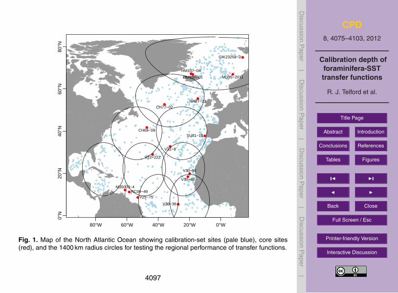
We used the 862-site north Atlantic planktonic foraminifera calibration-set compiledby Kucera et al. (2005) (Fig. 1). Ocean temperatures were extracted from the WorldOcean Atlas (WOA, 1998), interpolated to the calibration-set observations. We usedthe caloric warm and cold season, and mean annual temperatures at the 14 standard5

WOA depths between the surface and 500 m.Sixteen planktonic foraminifera assemblage time series straddling the last termina-

tion from the N Atlantic were compiled and their taxonomy harmonised to match thecalibration-set (Table 1, Fig. 1). The following selection criteria were used: foraminiferacounted in the greater than 150 µm fraction to match the calibration-set, resulting in the10

rejection of some high-latitude sites; core location north of 5◦ N to avoid the edge of thecalibration-set; cores should span the last termination, with several observations fromboth the Holocene and the deglaciation with a temporal resolution of ∼one observationper millennium or better.

The SST reconstructions were derived for each depth and season using the mod-15

ern analogue technique (MAT) with five analogues (between four and six analogues,depending on depth and season, gave the lowest root mean square error of predic-tion) and squared chord distances (Prell, 1985). Performance of the transfer functionswas estimated using leave-one-out cross-validation, and is reported both for the wholeNorth Atlantic Ocean and for nine arbitrarily defined 1400 km-radius regions covering20

the North Atlantic.Reconstructions of warm and cold season temperature at WOA standard depths

from the surface down to 500 m were calculated using MAT. We attempt to determinethe season and depth at which temperature variability appears to be most important byusing a constrained ordination to find the proportion of the variance in the fossil data25

explained by each reconstruction (Telford and Birks, 2011). We assume that recon-structions that explain least variance in the fossil data are probably from depths thatdid not drive the variability in the fossil data. We used redundancy analysis (Rao, 1964)

4079





CPD8, 4075–4103, 2012



Title Page



Tables Figures

J I

J I

Back Close

Full Screen / Esc



Discussion

Paper

|D

iscussionP

aper|

Discussion

Paper

|D

iscussionP

aper|

for the constrained ordination because the taxonomic turnover in the cores is relativelysmall. The statistical significance of the reconstructions was assessed by testing if theyexplained significantly more of the variance than a null model of 999 transfer functionstrained on random data (Telford and Birks, 2011). We used a white noise null modelbecause of the complexity of generating spatially autocorrelated random data with the5

correct spatial structure for each environmental variable. Our 95 % significance levelwill thus be liberal.

We used the output from simulations of LGM and pre-industrial (PI) climate per-formed by four coupled climate models participating in the Coupled Model Intercom-parison Project CMIP5 to identify areas of the N Atlantic LGM that have poor thermal10

analogues in the PI ocean. The models included in the analysis are listed in Table 2; theLGM and PI simulations were performed in compliance with PMIP3 protocol. Completedocumentation of the models and experimental setup can be found on the PMIP3 web-site (http://pmip3.lsce.ipsl.fr/). We generated monthly climatologies for 50 yr periods ofthe LGM and PI simulations. For each model, we interpolated July temperatures in ev-15

ery grid box to 10 m intervals in the top 300 m of the ocean, and found the Euclideandistance from the simulated LGM ocean to the most similar grid box in the simulatedPI ocean.

All analyses were run using the R statistical language version 2.14.1 (R DevelopmentCore Team, 2011). Reconstructions were generated with the rioja package version 0.7-20

3 (Juggins, 2012); the statistical significance and importance of reconstructions wastested with the palaeoSig package version 1.1-1 (Telford, 2012); redundancy analysiswas fitted with the vegan package version 2.0-2 (Oksanen et al., 2011).

3 Results

Planktonic foraminifera-SST transfer function performance for the whole North Atlantic25

Ocean is best near the surface for the cold season and the annual mean temperature(Fig. 2). The warm season has a maximum r2 between 30 m and 50 m. This result is

4080





http://pmip3.lsce.ipsl.fr/

CPD8, 4075–4103, 2012



Title Page



Tables Figures

J I

J I

Back Close

Full Screen / Esc



Discussion

Paper

|D

iscussionP

aper|

Discussion

Paper

|D

iscussionP

aper|

similar to that of Pflaumann et al. (1996), who only considered the top 75 m, confirmingthat their result was not an artefact of the SIMMAX method (Telford et al., 2004) orthe older, less precise SST data they use (Levitus, 1982). This would seem to supportthe current practice of attributing transfer function results to a fixed depth representingthe mixed layer. However, different patterns emerge when performance of the transfer5

functions in different regions is estimated (Fig. 3). In several regions, there is a pro-nounced drop in r2 near the surface during the warm season, and in the tropics this isalso found for the cold season and the annual mean temperature. This result suggeststhat the near monotonic decline in r2 with depth for the cold season and annual meantemperature in the whole North Atlantic is, at least in part, an artefact of mixing together10

different regions with different depth sensitivities.The regional differences in the performance of transfer functions with depth are re-

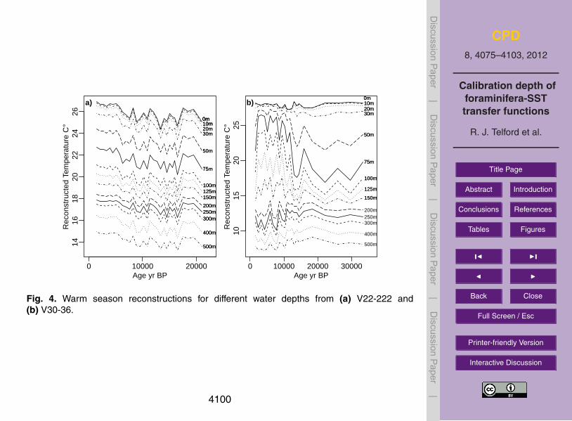
flected in the time series of reconstructions at different depths. For cores north of 25◦ N,the reconstructions from different depths and seasons resemble one another, with anoffset (Fig. 4a). Tropical cores have very different reconstructions for different depths.15

For example, near-surface temperature reconstructions from site V30-36 (Fig. 4b) in-dicate little variability over the last 30 000 yr, whereas reconstructions from 75 m and100 m depth suggest a warming from the glacial into the Holocene of over 5 ◦C andreconstructions from greater depths have less variability, with a cooling of up to 2 ◦C.

The difference between reconstructions at different depths in the time series is man-20

ifested in the proportion of the variance in the fossil data that they explain (Fig. 5).The profile of variance in the fossil data explained by temperature reconstructions atdifferent water depths and seasons varies geographically (Fig. 5).

The four sites in the Nordic Seas have similar shaped profiles (Fig. 5a–d). Theamount of variance explained is generally high for the top 200–300 m, and declines25

steeply below this. Towards the surface, the variance explained by warm season recon-structions declines and usually falls below values for the cold season reconstructions.At about 200 m, the warm season explains slightly more than the cold season.

4081





CPD8, 4075–4103, 2012



Title Page



Tables Figures

J I

J I

Back Close

Full Screen / Esc



Discussion

Paper

|D

iscussionP

aper|

Discussion

Paper

|D

iscussionP

aper|

The three sites in the North Atlantic Drift (Fig. 5e–g) mostly have broad peaks inthe amount of variance explained by warm season reconstructions, with a maximumat about 200 m. The amount of variance explained by the cold season reconstructionshas a flatter profile, and explains less than that explained by the warm season at itsmaximum. At these sites, all reconstructions are statistically significant.5

The single site off the Portuguese margin (Fig. 5h) has a unique profile, with theamount of variance explained by the reconstructions slowly increasing with increasingdepth.

The two sites in the North Atlantic subtropical gyre have idiosyncratic profiles(Fig. 5i–j). The amount of variance explained by reconstructions at V32-8 is greatest10

in the warm season at the surface, and declines with depth until reconstructions arenot statistically significant below about 200 m. At V22-222 the pattern is more complex,with the warm season reconstruction explaining more at about 75 m than at the sur-face, below this the amount explained falls, and then rises again, but the magnitude ofthe changes is small. The amount of variance explained by the cold season is similar,15

except it does not show the near surface decline. All reconstructions at this site arestatistically significant.

Both the patterns in variance explained and the significance level changes southof 25◦ N. The two sites near the West African upwelling cells (Fig. 5k–l) both havenear surface reconstructions that explain the most variance, with the warm season20

explaining more than the cold. Reconstructions of subsurface temperatures explainvery little variance, but deeper reconstructions explain more, especially at V30-49.

At the tropical sites (Fig. 5m–p), near-surface reconstructions explain little of the vari-ance and are typically not statistically significant. Sub-surface reconstructions explainabout twice as much of the variance as near-surface reconstruction, and are statis-25

tically significant or almost so. Reconstructions from deeper than 150 m also explainlittle variance and are not statistically significant. There is little difference between thewarm and cold seasons in the amount of variance explained.

4082





CPD8, 4075–4103, 2012



Title Page



Tables Figures

J I

J I

Back Close

Full Screen / Esc



Discussion

Paper

|D

iscussionP

aper|

Discussion

Paper

|D

iscussionP

aper|

Figure 6 shows, for each grid box, the Euclidean distance between the vertical tem-perature profiles in the top 300 m of the simulated LGM ocean and the most similarprofile in the PI. Large values indicate grid boxes that lack good analogues for the LGMthermal structure in the modern ocean. The spatial pattern is similar for all four CMIP5models (Fig. 6), with less good analogues in the Nordic Seas and around the Gulf5

Stream separation, and the worst analogues in the area south of the subtropical gyre.This inter-model consistency suggests that these are robust features.

4 Discussion

Planktonic foraminifera assemblages in the sediment integrate foraminiferal communi-ties from different seasons and water depths. Therefore their composition reflects the10

thermal structure of the entire upper ocean, so it would be surprising if reconstruc-tions of temperature from one depth in one season perfectly captured SST changesthrough space and time. As long as this thermal structure remains the same, transferfunctions based on a fixed calibration depth should not be affected. Our analysis ofNorth Atlantic foraminifera time series across the last termination (Figs. 4, 5) as well15

as model simulations of the LGM and PI (Fig. 6) indicate that ocean thermal structurehas changed and that transfer function-based reconstructions are affected. We findthat the depth at which planktonic foraminifera assemblages are usually calibrated to,10 m, is rarely the depth that explains the most variance in the fossil data in the NorthAtlantic. Given the ecological knowledge on the vertical and seasonal abundances of20

planktonic foraminifera (Chapman, 2010; Fairbanks et al., 1980), these results are notsurprising. They pose both opportunities and challenges for palaeoceanography, whichwe discuss below.

4083





CPD8, 4075–4103, 2012



Title Page



Tables Figures

J I

J I

Back Close

Full Screen / Esc



Discussion

Paper

|D

iscussionP

aper|

Discussion

Paper

|D

iscussionP

aper|

4.1 Opportunities

The greatest opportunity is the potential for more meaningful reconstructions, leadingto improved understanding of past climate. For example, the temperature reconstruc-tions from 10 m and 75 m at V30-36 (Fig. 4) are very different, suggesting either onlyminor temperature changes over the last 30 000 yr or pronounced variability. If strong5

subsurface cooling at the LGM can be reconstructed at other sites across the trop-ics, it will challenge the consensus that the tropical oceans only experienced moderatecooling at the LGM (MARGO Project Members, 2009).

Acknowledging that changes in foraminifera assemblages across the last termina-tion, in most of the North Atlantic, were more sensitive to subsurface conditions than10

surface conditions will allow greater insight into palaeoceanographic processes by ex-ploiting information on the seasonal and depth sensitivity of proxies. This has alreadybeen attempted, for example by Jansen et al. (2008) who examined the contrast-ing SST reconstructions from the Vøring Plateau in the Nordic seas: diatoms andalkonones reconstruct a warm early Holocene, whereas planktonic foraminifera SST15

reconstructions, both isotopic and faunal, are warmest in the late Holocene. Jansen etal. (2008) argued that alkenone and diatoms represent summer SST, while planktonicforaminifera represent sub-surface conditions and are sensitive to the temperature setduring winter ventilation. They concluded that the contrasting reconstructions indicatedthat direct enhanced insolation rather than advection of warm water was responsi-20

ble for the early Holocene thermal optima. Another study by Adloff et al. (2011) findsa discrepancy between climate model output and reconstructed SST for the EasternMediterranean during the early Holocene thermal optimum. They find that these datacan be reconciled by considering the foraminifera-derived reconstruction to representthe upper water column rather than just the surface.25

4084





CPD8, 4075–4103, 2012



Title Page



Tables Figures

J I

J I

Back Close

Full Screen / Esc



Discussion

Paper

|D

iscussionP

aper|

Discussion

Paper

|D

iscussionP

aper|

4.2 Challenges

The first challenge is to interpret the ambiguity in having multiple reconstructions, onefor each depth and season examined. There may be a desire to try to attach palaeocli-mate meaning to several, or indeed all of these. For example, the record from V30-36(Fig. 4b) could be interpreted as having little temperature change at the surface, but5

pronounced temperature changes subsurface. However, it is unlikely that there is suf-ficient information in the fossil data to reconstruct several independent variables simul-taneously (Telford and Birks, 2011). Therefore, at any given time, it is likely that onlyone of the multiple reconstructions can be considered. The statistical significance ofeach reconstruction may help guide the choice of which should be considered.10

The second challenge is that the depth and season that explains the most variancemay vary not only geographically but also with time at one site. Here we consider as-semblage changes over the last termination. Different patterns may have been foundif we had considered only Interglacial or only Glacial periods. Theoretically the frame-work we develop here could be used to explore this problem using a moving-window15

analysis, but there may be problems with obtaining adequate faunistic analogues.Other challenges include problems using and displaying this information. There is a

long tradition of drawing maps of SST anomalies (CLIMAP Project Members, 1976;MARGO Project Members, 2009). If reconstructions have to be made for differentdepths in different regions, producing such maps will be problematic. This does not20

reduce the utility of the reconstructions for comparing with climate model output.Planktonic foraminifera assemblage-based SST reconstructions have traditionally

been assigned a priori to a fixed depth, typically 10 m. This contrasts with recon-structions based on foraminifera geochemistry, where the temperature change in theforaminiferas’ habitat may be possible to reconstruct accurately, but the depth and sea-25

son which this represents is unclear a priori and needs to be estimated post hoc. Ourresults suggest that assignment of the signal in assemblage-based reconstructions toa particular depth and season needs to be treated in a similar manner to the geochem-istry data.

4085





CPD8, 4075–4103, 2012



Title Page



Tables Figures

J I

J I

Back Close

Full Screen / Esc



Discussion

Paper

|D

iscussionP

aper|

Discussion

Paper

|D

iscussionP

aper|

4.3 Implications

If palaeoceanographic change can be thought of as geographically redistributing, ex-panding and contracting water masses with certain fixed thermal properties, our re-sults are but a curiosity. In this case, in a given water mass, the surface temperature istied to the subsurface temperature which the foraminifera are responding to, so a sur-5

face reconstruction will be valid because of this correlation. Our comparison of CMIP5LGM and PI ocean temperature data demonstrates that this simplistic notion of cli-mate change is incorrect. In the model output, much of the tropical North Atlantic hasa thermal structure in the LGM that is not found in the PI ocean. It is here that theconsequences of foraminifera being sensitive to subsurface rather than surface tem-10

peratures are likely to be most severe, and it is here where reconstructions from dif-ferent depths differ most. Perhaps not coincidently, the tropical ocean is where thereis a large mismatch between climate model output and proxy data (Otto-Bliesner etal., 2009). For example, proxy data show an east-west gradient in the size of the LGMtemperature anomaly in the tropical Atlantic which is not replicated in the model out-15

put (Otto-Bliesner et al., 2009). Our results suggesting large subsurface cooling in thewestern tropical Atlantic, suggests that this result may need revisiting.

The non-analogue ocean thermal structure has two consequences for planktonicforaminifera assemblage-based reconstructions: first that the uncertainty in the tropicalreconstructions is likely to be underestimated, and second that reconstructions are20

likely to be biased. Therefore, we need to consider the sign and likely magnitude of thisbias.

If the thermal gradient was shallower in the past, subsurface temperatures now as-sociated with warm surface conditions would have been associated with cooler SST inthe past (Fig. 7). Consequently, foraminifera assemblages now associated with warm25

SSTs because of their relationship with cooler subsurface conditions will in the pasthave been associated with cooler SSTs, and reconstructions will have a warm bias.

4086





CPD8, 4075–4103, 2012



Title Page



Tables Figures

J I

J I

Back Close

Full Screen / Esc



Discussion

Paper

|D

iscussionP

aper|

Discussion

Paper

|D

iscussionP

aper|

Conversely, if the thermal gradient was steeper, SST reconstructions will have a coldbias.

Our reconstructions using transfer functions calibrated against different depths showsubsurface marked cooling at some tropical sites, in contrast to previous reconstructionof a modest cooling. If this bias is widespread in tropical sites it may likely sufficient to5

produce a bias in estimates of climate sensitivity based on the difference betweenLGM and modern climate. A sensitivity study undertaken by Schmittner et al. (2011)found that a global 0.5 ◦C bias in LGM ocean anomalies gave a 1 ◦C change in climatesensitivity. Because the sign of the bias in the SST reconstruction may vary by region,we cannot estimate the sign or magnitude of the global mean bias.10

There has been some debate about which season planktonic foraminifera assem-blages can be used to reconstruct (Kucera et al., 2005). Our results render this debatelargely moot, as they show that the signal in the foraminfera assemblage data is usuallyfrom the subsurface where seasonality is subdued relative to the surface.

4.4 Solutions15

The obvious solution to the problem of planktonic foraminifera being sensitive to sub-surface rather than near surface temperatures in much of the North Atlantic would seemto be to calibrate planktonic foraminifera assemblages against a different, more eco-logically relevant depth. This has been done, for example by Andersson et al. (2010)who reconstructed 100 m SST. Reconstructions of subsurface conditions could be in-20

terpreted in much the same way as surface reconstructions, and could be used as atarget for estimating climate sensitivity. However, the most ecologically relevant depthvaries in space and time, and the assemblages will probably integrate the commu-nities from several depths and seasons, so selecting a more appropriate fixed depthfor temperature reconstructions for each location is probably not trivial and does not25

completely circumvent the problem. The method we develop here can only be used toidentify the most relevant depth from time series. It cannot be used for single assem-blages.

4087





CPD8, 4075–4103, 2012



Title Page



Tables Figures

J I

J I

Back Close

Full Screen / Esc



Discussion

Paper

|D

iscussionP

aper|

Discussion

Paper

|D

iscussionP

aper|

Since the most appropriate depth probably changes with time, it might be useful totry to identify the most appropriate depth for each time period in each assemblage timeseries with a moving window analysis rather than using a single fixed depth. Assigningthe signal in the assemblage data to a dynamic rather than fixed depth is probably nottractable. It will be difficult to demarcate periods where specific depths are optimal, and5

assemblages with poor analogues in the modern ocean may generate spurious results.An alternative solution is to use forward modelling, ecological models that predict the

planktonic foraminifera assemblages given the output of a climate model. The matchbetween the fossil assemblage and the model assemblage could then be assessed.Forward modelling of planktonic foraminifera assemblages has been developed by10

Fraile et al. (2008) and Lombard et al. (2011). Ideally forward models of foraminiferaassemblages would be run in conjunction with forward modelling of the geochemistryof planktonic foraminiferal tests (Schmidt and Mulitza, 2002) for a comprehensive so-lution. Forward models of planktonic foraminifera assemblages are not yet sufficientlydeveloped for assessing the fit between observed and modelled assemblages, for ex-15

ample they include only a subset of taxa. A more achievable short-term goal is to useforward models of foraminifera assemblages to help constrain the sign and likely mag-nitude of biases in SST reconstructions. Transfer functions, calibrated against 10 mSST, could be generated for simulated foraminifera assemblages forced by PI climatemodel output. These transfer functions could be used to reconstruct SST from simu-20

lated foraminifera assemblages forced by LGM conditions, and the spatial extent, signand magnitude of any bias in the reconstructions determined.

Another solution is to try to constrain foraminifera assemblage-based estimates ofSST with other proxies. If proxies that represent different depth are compared, anydiscrepancies may indicate periods when the thermal structure of the upper ocean25

changed. However, discrepancies could also be due to changing seasonality of theproduction of the proxies (Chapman et al., 1996).

4088





CPD8, 4075–4103, 2012



Title Page



Tables Figures

J I

J I

Back Close

Full Screen / Esc



Discussion

Paper

|D

iscussionP

aper|

Discussion

Paper

|D

iscussionP

aper|

4.5 Other proxies

The potential biases we discuss in this paper for planktonic foraminifera assemblage-based SST reconstructions in the North Atlantic will apply to other oceans and someother proxies. Assemblage or geochemistry data from taxa that are constrained tolive in the photic zone because they, or their symbionts, are photosynthetic, for ex-5

ample diatoms (Koc Karpuz and Schrader, 1990), can be used to calculate surfacetemperatures, but may generate biased results if the seasonality of the proxy produc-tion changes. Other micropalaeontological proxies that are not constrained to live inthe photic zone, for example radiolarians (Pisias et al., 1997), risk the same biases asplanktonic foraminifera transfer functions if the ocean thermal structure changes.10

Estimates of SST from geochemical proxies on subsurface micropalaeontologicalproxies may also be biased. Mg/Ca ratios and δ18O of foraminiferal tests may accu-rately record temperature at the time and depth of calcification, but if the seasonalityor depth of calcification has changed, or the ocean thermal structure has changed,estimates of SST will be biased.15

5 Conclusions

We present evidence that planktonic foraminifera assemblages are usually more sensi-tive to subsurface temperatures than the 10 m SST they are usually calibrated against.Consequently, reconstructions of 10 m SST are likely to be biased, especially in thetropics where non-analogue ocean thermal structures occurred in the LGM. The sign20

and magnitude of the bias is likely to vary regionally, probably with a warm bias in thetropical N Atlantic. Foraminifera-based reconstructions for other ocean basins need tobe assessed.

This problem exposes the limitations of using transfer functions to reconstruct pastclimate to compare with model output. The most promising solution is to use forward25

4089





CPD8, 4075–4103, 2012



Title Page



Tables Figures

J I

J I

Back Close

Full Screen / Esc



Discussion

Paper

|D

iscussionP

aper|

Discussion

Paper

|D

iscussionP

aper|

models of planktonic foraminifera assemblages which can be directly compared withobserved fossil foraminifera assemblages, however considerable work is needed todevelop these models.

Acknowledgements. We acknowledge the World Climate Research Programme’s WorkingGroup on Coupled Modelling, which is responsible for CMIP, and we thank the climate mod-5

elling groups listed in Table 2 for producing and making available their model output. For CMIPthe US Department of Energy’s Program for Climate Model Diagnosis and Intercomparison pro-vides coordinating support and led development of software infrastructure in partnership withthe Global Organization for Earth System Science Portals. We thank the foraminifera analystswhose data we used.10

Norwegian Research Council FriMedBio project palaeoDrivers (213607) helped support thiswork. CL acknowledges the support of the Centre for Climate Dynamics (SKD) at the BjerknesCentre. This is publication no. A402 from the Bjerknes Centre for Climate Research.

References

Adloff, F., Mikolajewicz, U., Kucera, M., Grimm, R., Maier-Reimer, E., Schmiedl, G., and Emeis,15

K.-C.: Upper ocean climate of the Eastern Mediterranean Sea during the Holocene InsolationMaximum – a model study, Clim. Past, 7, 1103–1122, doi:10.5194/cp-7-1103-2011, 2011.

Andersson, C., Pausata, F. S. R., Jansen, E., Risebrobakken, B., and Telford, R. J.: Holocenetrends in the foraminifer record from the Norwegian Sea and the North Atlantic Ocean, Clim.Past, 6, 179–193, doi:10.5194/cp-6-179-2010, 2010.20

Birks, H. J. B., Heiri, O., Seppa, H., and Bjune, A.: Strengths and weaknesses of quantitativeclimate reconstructions based on Late-Quaternary biological proxies, Open Ecol. J., 3, 68–110, 2010.

Braconnot, P., Harrison, S. P., Kageyama, M., Bartlein, P. J., Abe-Ouchi, V. M.-D. A., Otto-Bliesner, B., and Zhao, Y.: Evaluation of climate models using palaeoclimatic data, Nat. Clim.25

Change, 2, 417–424, doi:10.1038/nclimate1456, 2012.Chapman, M. R.: Seasonal production patterns of planktonic foraminifera in the NE Atlantic

Ocean: Implications for paleotemperature and hydrographic reconstructions, Paleoceanog-raphy, 25, PA1101, doi:10.1029/2008pa001708, 2010.

4090





http://dx.doi.org/10.5194/cp-7-1103-2011

http://dx.doi.org/10.5194/cp-6-179-2010

http://dx.doi.org/10.1038/nclimate1456

http://dx.doi.org/10.1029/2008pa001708

CPD8, 4075–4103, 2012



Title Page



Tables Figures

J I

J I

Back Close

Full Screen / Esc



Discussion

Paper

|D

iscussionP

aper|

Discussion

Paper

|D

iscussionP

aper|

Chapman, M. R., Shackleton, N. J., Zhao, M., and Eglinton, G.: Faunal and alkenone recon-structions of subtropical North Atlantic surface hydrography and paleotemperature over thelast 28 kyr, Paleoceanography, 11, 343–357, 1996.

Cleroux, C., Lynch-Stieglitz, J., Schmidt, M. W., Cortijo, E., and Duplessy, J.-C.: Evidencefor calcification depth change of Globorotalia truncatulinoides between deglaciation and5

Holocene in the Western Atlantic Ocean, Mar. Micropaleontol., 73, 57–61, 2009.CLIMAP Project Members: The surface of the ice-age Earth, Science, 191, 1131–1137, 1976.Duplessy, J.-C., Labeyrie, L., Arnold, M., Paterne, M., Duprat, J., and van Weering, T. C. E.:

Changes in surface salinity of the North Atlantic Ocean during the last deglaciation, Nature,358, 485–488, 1992.10

Fairbanks, R. G., Wiere, P. H., and Be, A. W. H.: Vertical distribution and isotopic compositionof living planktonic foraminifera in the Western North Atlantic, Science, 207, 61–63, 1980.

Fraile, I., Schulz, M., Mulitza, S., and Kucera, M.: Predicting the global distribution ofplanktonic foraminifera using a dynamic ecosystem model, Biogeosciences, 5, 891–911,doi:10.5194/bg-5-891-2008, 2008.15

Hegerl, G. C., Zwiers, F. W., Braconnot, P., Gillett, N. P., Luo, Y., Marengo Orsini, J. A., Nicholls,N., Penner, J. E., and Stott, P. A.: Understanding and Attributing Climate Change, in: ClimateChange 2007: The Physical Science Basis. Contribution of Working Group I to the FourthAssessment Report of the Intergovernmental Panel on Climate Change, edited by: Solomon,S., Qin, D., Manning, M., Chen, Z., Marquis, M., Averyt, K. B., Tignor, M., and Miller, H. L.,20

Cambridge University Press, Cambridge, United Kingdom and New York, NY, USA, 2007.Huls, M.: Distribution of planktic foraminifera of sediment core M35003-4,

doi:10.1594/PANGAEA.55756, 1999.Jansen, E., Andersson, C., Moros, M., Nisancioglu, K. H., Nyland, B. F., and Telford, R. J.: The

early to mid-Holocene thermal optimum in the North Atlantic, in: Natural Climate Variability25

and Global Warming – A Holocene Perspective, edited by: Battarbee, R. W. and Binney, H.A., Wiley-Blackwell, Chichester, 123–137, 2008.

Juggins, S.: rioja: An R Package for the Analysis of Quaternary Science Data, Version 0.7-3.,2012.

Knudsen, K. L., Jiang, H., Jansen, E., Eirıksson, J., Heinemeier, J., and Seidenkrantz, M.30

S.: Environmental changes off North Iceland during the deglaciation and the Holocene:foraminifera, diatoms and stable isotopes, Mar. Micropaleontol., 50, 273–305, 2004.

4091





http://dx.doi.org/10.5194/bg-5-891-2008

http://dx.doi.org/10.1594/PANGAEA.55756

CPD8, 4075–4103, 2012



Title Page



Tables Figures

J I

J I

Back Close

Full Screen / Esc



Discussion

Paper

|D

iscussionP

aper|

Discussion

Paper

|D

iscussionP

aper|

Knutti, R. and Hegerl, G. C.: The equilibrium sensitivity of the Earth’s temperature to radiationchanges, Nat. Geosci., 1, 735–743, doi:10.1038/ngeo337, 2008.

Koc Karpuz, N. and Schrader, H.: Surface sediment diatom distribution and Holocene pale-otemperature variations in the Greenland, Iceland and Norwegian Sea, Paleoceanography,5, 557–580, doi:10.1029/PA005i004p00557, 1990.5

Kucera, M., Weinelt, M., Kiefer, T., Pflaumann, U., Hayes, A., Weinelt, M., Chen, M.-T., Mix,A. C., Barrows, T. T., Cortijo, E., Duprat, J., Juggins, S., and Waelbroeck, C.: Reconstruc-tion of the glacial Atlantic and Pacific sea-surface temperatures from assemblages of plank-tonic foraminifera: multi-technique approach based on geographically constrained calibrationdatasets, Quaternary Sci. Rev., 24, 951–998, doi:10.1016/j.quascirev.2004.07.017, 2005.10

Labeyrie, L., Leclaire, H., Waelbroeck, C., Cortijo, E., Duplessy, J.-C., Vidal, L., Elliot, M.,LeCoat, B., and Auffret, G.: Temporal variability of the surface and deep waters of the NorthWest Atlantic Ocean at orbital and millennial scales, in: Mechanisms of global climate changeat millennial time scales, edited by: Webb, R., Clark, P. U., and Keigwin, L. D., GeophysicalMonograph, American Geophysical Union, 77–98, 1999.15

Levitus, S.: Climatological atlas of the world ocean, NOAA Prof. Pap., 13, 1–173, 1982.Lombard, F., Labeyrie, L., Michel, E., Bopp, L., Cortijo, E., Retailleau, S., Howa, H., and Joris-

sen, F.: Modelling planktic foraminifer growth and distribution using an ecophysiological multi-species approach, Biogeosciences, 8, 853–873, doi:10.5194/bg-8-853-2011, 2011.

Lynch-Stieglitz, J., Curry, W. B., and Slowey, N.: Weaker Gulf Stream in the Florida Straits20

during the Last Glacial Maximum, Nature, 402, 644–648, 1999.Marchal, O., Cacho, I., Stocker, T. F., Grimalt, J. O., Calvo, E., Martrat, B., Shackleton, N.,

Vautravers, M., Cortijo, E., van Kreveld, S., Andersson, C., Koc, N., Chapman, M., Sbaffi, L.,Duplessy, J.-C., Sarnthein, M., Turon, J.-L., Duprat, J., and Jansen, E.: Apparent long-termcooling of the sea surface in the northeast Atlantic and Mediterranean during the Holocene,25

Quaternary Sci. Rev., 21, 455–483, 2002.MARGO Project Members: Constraints on the magnitude and patterns of ocean cooling at the

Last Glacial Maximum, Nat. Geosci., 2, 127–132, doi:10.1038/ngeo411, 2009.Mix, A. C.: Percentages of planktonic foraminifera species in sediment core V32-8,

doi:10.1594/PANGAEA.355352, 2006a.30

Mix, A. C.: Percentages of planktonic foraminifera species in sediment core V22-222,doi:10.1594/PANGAEA.355340, 2006b.

4092





http://dx.doi.org/10.1038/ngeo337

http://dx.doi.org/10.1029/PA005i004p00557

http://dx.doi.org/10.1016/j.quascirev.2004.07.017

http://dx.doi.org/10.5194/bg-8-853-2011

http://dx.doi.org/10.1038/ngeo411



CPD8, 4075–4103, 2012



Title Page



Tables Figures

J I

J I

Back Close

Full Screen / Esc



Discussion

Paper

|D

iscussionP

aper|

Discussion

Paper

|D

iscussionP

aper|

Mix, A. C.: Percentages of planktonic foraminifera species in sediment core V30-51,doi:10.1594/PANGAEA.355351, 2006c.

Mix, A. C.: Percentages of planktonic foraminifera species in sediment core V30-49,doi:10.1594/PANGAEA.355350, 2006d.

Mix, A. C.: Percentages of planktonic foraminifera species in sediment core RC09-49,5

doi:10.1594/PANGAEA.355331, 2006e.Mix, A. C.: Percentages of planktonic foraminifera species in sediment core V25-75,

doi:10.1594/PANGAEA.355345, 2006f.Mix, A. C.: Percentages of planktonic foraminifera species in sediment core V30-36,

doi:10.1594/PANGAEA.355347, 2006g.10

Murray, J.: On the distribution of the pelagic foraminifera at the surface and on the floor of theocean, National Science, 11, 17–27, 1897.

Oksanen, J., Blanchet, F. G., Kindt, R., Legendre, P., Minchin, P. R., O’Hara, R. B., Simpson,G. L., Solymos, P., Stevens, M. H. H., and Wagner, H.: vegan: Community Ecology Package.R package version 2.0-2, 2011.15

Otto-Bliesner, B. L., Schneider, R., Brady, E. C., Kucera, M., Abe-Ouchi, A., Bard, E., Braconnot,P., Crucifix, M., Hewitt, C. D., Kageyama, M., Marti, O., Paul, A., Rosell-Mele, A., Waelbroeck,C., Weber, S. L., Weinelt, M., and Yu, Y.: A comparison of PMIP2 model simulations and theMARGO proxy reconstruction for tropical sea surface temperatures at last glacial maximum,Clim. Dynam., 32, 799–815, doi:10.1007/s00382-008-0509-0, 2009.20

Pflaumann, U., Duprat, J., Pujol, C., and Labeyrie, L. D.: SIMMAX: A modern analog tech-nique to deduce Atlantic sea surface temperatures from planktonic foraminifera in deep-seasediments, Paleoceanography, 11, 15–35, doi:10.1029/95pa01743, 1996.

Pisias, N. G., Roelofs, A., and Weber, M.: Radiolarian-based transfer functions for estimatingmean surface ocean temperatures and seasonal range, Paleoceanography, 12, 365–379,25

doi:10.1029/97PA00582, 1997.Prell, W. L.: The stability of low-latitude sea-surface temperatures: An evaluation of the CLIMAP

reconstruction with emphasis on the positive SST anomalies, Department of Energy, Wash-ington, DC, 60 pp., 1985.

R Development Core Team: R: A language and environment for statistical computing., R Foun-30

dation for Statistical Computing, Vienna, Austria, 2011.Rao, C. R.: The use and interpretation of principal component analysis in applied research,

Sankhya Ser. A, 26, 329–358, 1964.

4093










http://dx.doi.org/10.1007/s00382-008-0509-0

http://dx.doi.org/10.1029/95pa01743

http://dx.doi.org/10.1029/97PA00582

CPD8, 4075–4103, 2012



Title Page



Tables Figures

J I

J I

Back Close

Full Screen / Esc



Discussion

Paper

|D

iscussionP

aper|

Discussion

Paper

|D

iscussionP

aper|

Risebrobakken, B., Jansen, E., Andersson, C., Mjelde, E., and Hevroy, K.: Planktonicforaminiferal and stable oxygen isotope record of Holocene sediments from the NorwegianSea, doi:10.1594/PANGAEA.760166, Supplement to: Risebrobakken et al. (2003): A high-resolution study of Holocene paleoclimatic and paleoceanographic changes in the NordicSeas, Paleoceanography, 18, 1017, doi:10.1029/2002PA000764, 2003.5

Sachs, H. M., Webb, T., and Clark, D. R.: Paleoecological Transfer Functions, Annu. Rev. EarthPl. Sc., 5, 159–178, doi:10.1146/annurev.ea.05.050177.001111, 1977.

Sarnthein, M., van Kreveld, S. A., Erlenkeuser, H., Grootes, P. M., Kucera, M., Pflau-mann, U., and Schulz, M.: Distribution of foraminifera of sediment core GIK23258-2,doi:10.1594/PANGAEA.114682, Supplement to: Sarnthein et al. (2003): Centennial-to-10

millennial-scale periodicities of Holocene climate and sediment injections off western Bar-ents shelf, 75◦ N, Boreas, 32, 447–461, doi:10.1111/j.1502-3885.2003.tb01227.x, 2003.

Schmidt, G. A. and Mulitza, S.: Global calibration of ecological models for planktic foraminiferafrom coretop carbonate oxygen-18, Mar. Micropaleontol., 44, 125–140, 2002.

Schmittner, A., Urban, N. M., Shakun, J. D., Mahowald, N. M., Clark, P. U., Bartlein, P. J., Mix, A.15

C., and Rosell-Mele, A.: Climate Sensitivity Estimated from Temperature Reconstructions ofthe Last Glacial Maximum, Science, 334, 1385–1388, doi:10.1126/science.1203513, 2011.

Telford, R. J.: palaeoSig: Significance Tests of Quantitative Palaeoenvironmental Reconstruc-tions, R package version 1.1., 2012.

Telford, R. J. and Birks, H. J. B.: The secret assumption of transfer functions: problems with20

spatial autocorrelation in evaluating model performance, Quaternary Sci. Rev., 24, 2173–2179, doi:10.1016/j.quascirev.2005.05.001, 2005.

Telford, R. J. and Birks, H. J. B.: A novel method for assessing the statistical significanceof quantitative reconstructions inferred from biotic assemblages, Quaternary Sci. Rev., 30,1272–1278, 2011.25

Telford, R. J., Andersson, C., Birks, H. J. B., and Juggins, S.: Biases in the estimation of trans-fer function prediction errors, Paleoceanography, 19, PA4014, doi:10.1029/2004pa001072,2004.

WOA: World Ocean Atlas 1998 Version 2, National Oceanographic Data Center, Silver Spring,Maryland, 1998.30

4094






http://dx.doi.org/10.1029/2002PA000764

http://dx.doi.org/10.1146/annurev.ea.05.050177.001111


http://dx.doi.org/10.1111/j.1502-3885.2003.tb01227.x

http://dx.doi.org/10.1126/science.1203513

http://dx.doi.org/10.1016/j.quascirev.2005.05.001

http://dx.doi.org/10.1029/2004pa001072

CPD8, 4075–4103, 2012



Title Page



Tables Figures

J I

J I

Back Close

Full Screen / Esc



Discussion

Paper

|D

iscussionP

aper|

Discussion

Paper

|D

iscussionP

aper|

Table 1. Cores used in the analyses, listed from north to south.

Core Location Number of Timespan Referenceobservations (kyr BP)

GIK23258-2 14◦ E 75◦ N 285 1–14 Sarnthein et al. (2003)HM107-04 19.1◦ W 67.2◦ N 92 0–13 Knudsen et al. (2004)MD95-2011 7.6◦ E 67◦ N 380 0–14 Risebrobakken et al. (2003)HM107-05 17.9◦ W 66.9◦ N 56 0–16 Knudsen et al. (2004)NA87-22 14.7◦ W 55.5◦ N 104 1–14 Duplessy et al. (1992)CH77-02 36.1◦ W 52.7◦ N 153 0–12 Marchal et al. (2002)CH69-09 47.4◦ W 41.8◦ N 58 1–17 Labeyrie et al. (1999)SU81-18 10.2◦ W 37.8◦ N 41 0–21 Duplessy et al. (1992)V32-8 32.4◦ W 32.8◦ N 25 2–23 Mix (2006a)V22-222 43.6◦ W 28.9◦ N 30 2–21 Mix (2006b)V30-51 19.9◦ W 19.9◦ N 18 2–32 Mix (2006c)V30-49 21.1◦ W 18.4◦ N 26 2–23 Mix (2006d)M35003-4 61.2◦ W 12.1◦ N 76 0–23 Huls (1999)RC09-49 58.6◦ W 11.2◦ N 22 2–22 Mix (2006e)V25-75 53.2◦ W 8.6◦ N 35 2–28 Mix (2006f)V30-36 27.3◦ W 5.3◦ N 23 2–33 Mix (2006g)

4095





CPD8, 4075–4103, 2012



Title Page



Tables Figures

J I

J I

Back Close

Full Screen / Esc



Discussion

Paper

|D

iscussionP

aper|

Discussion

Paper

|D

iscussionP

aper|

Table 2. CMIP5 coupled models used in this analysis. The sponsoring institutions of the modelsare: GISS-E2-R, NASA/GISS Goddard Institute for Space Studies, USA; MIROC-ESM, Centerfor Climate System Research (University of Tokyo), National Institute for Environmental Studies,and Frontier Research Center for Global Change (JAMSTEC), Japan; IPSL-CM5A-LR, InstitutPierre Simon Laplace, France; and MPI-ESM-P, Max Planck Institute for Meteorology, Germany.

Model Atmosphere Ocean Simulation period(years)

GISS-E2-R 2◦ ×2.5◦ ×L40 1◦ ×1.25◦ ×L32 PI: 4481–4530LGM: 3050–3099

MIROC-ESM T42 (∼ 2.8◦)×L80 0.5◦–1.7◦ ×1.4◦ ×L44 PI: 2280–2329LGM: 4648–4699

IPSL-CM5A-LR 3.75◦ ×1.9◦ ×L39 2◦ ×2◦ ×L31 PI: 2750–2799LGM: 2751–2800

MPI-ESM-P T63 (∼ 1.9◦)×L47 1.5◦ ×1.5◦ ×L40 PI: 2930–2979LGM: 1850–1899

4096





CPD8, 4075–4103, 2012



Title Page



Tables Figures

J I

J I

Back Close

Full Screen / Esc



Discussion

Paper

|D

iscussionP

aper|

Discussion

Paper

|D

iscussionP

aper|

GIK23258−2

HM107−04

MD95−2011HM107−05

NA87−22

CH77−02

CH69−09SU81−18

V32−8

V22−222

V30−51

V30−49

M35003−4RC09−49

V25−75

V30−36

80°W 60°W 40°W 20°W 0°W

0°N

20°N

40°N

60°N

80°N

Fig. 1. Map of the North Atlantic Ocean showing calibration-set sites (pale blue), core sites(red), and the 1400 km radius circles for testing the regional performance of transfer functions.

4097





CPD8, 4075–4103, 2012



Title Page



Tables Figures

J I

J I

Back Close

Full Screen / Esc



Discussion

Paper

|D

iscussionP

aper|

Discussion

Paper

|D

iscussionP

aper|

0 100 200 300 400 500

0.96

0.97

0.98

0.99

Depth m

r2

SummerWinterAnnual

Fig. 2. Transfer function performance for the whole North Atlantic calibration-set, shown as ther2 between measured and predicted temperatures for different depths and seasons.

4098





CPD8, 4075–4103, 2012



Title Page



Tables Figures

J I

J I

Back Close

Full Screen / Esc



Discussion

Paper

|D

iscussionP

aper|

Discussion

Paper

|D

iscussionP

aper|

0 100 200 300 400 500

0.0

0.2

0.4

0.6

0.8

Depth m

r2

3.5°W 72°N

0 100 200 300 400 500

0.0

0.2

0.4

0.6

0.8

Depth m

r2

32.5°W 54.5°N

0 100 200 300 400 500

0.0

0.2

0.4

0.6

0.8

Depth m

r2

25°W 39°N

0 100 200 300 400 500

0.0

0.2

0.4

0.6

0.8

Depth m

r2

54°W 39°N

0 100 200 300 400 500

0.0

0.2

0.4

0.6

0.8

Depth m

r2

24°W 22°N

0 100 200 300 400 500

0.0

0.2

0.4

0.6

0.8

Depth m

r2

49°W 22°N

0 100 200 300 400 500

0.0

0.2

0.4

0.6

0.8

Depth m

r2

75°W 22°N

0 100 200 300 400 500

0.0

0.2

0.4

0.6

0.8

Depth m

r2

20°W 7°N

0 100 200 300 400 500

0.0

0.2

0.4

0.6

0.8

Depth m

r2

40°W 7°N

Fig. 3. Transfer function performance, shown as the r2 between measured and predicted tem-peratures for different depths and seasons, for sites in different 1400 km radius regions (seeFig. 1) of the North Atlantic calibration-set. Legend as Fig. 2.

4099





CPD8, 4075–4103, 2012



Title Page



Tables Figures

J I

J I

Back Close

Full Screen / Esc



Discussion

Paper

|D

iscussionP

aper|

Discussion

Paper

|D

iscussionP

aper|

1416

1820

2224

26

Age yr BP

Rec

onst

ruct

ed T

empe

ratu

re C

°

0m10m20m30m

50m

75m

100m125m150m

200m250m300m

400m

500m

0m10m20m30m

50m

75m

100m125m150m

200m250m300m

400m

500m

0m10m

0 10000 20000

a)

1015

2025

Age yr BP

Rec

onst

ruct

ed T

empe

ratu

re C

°

0m10m20m30m

50m

75m

100m

125m

150m

200m250m300m

400m

500m

0m10m20m30m

50m

75m

100m

125m

150m

0 10000 20000 30000

b)

Fig. 4. Warm season reconstructions for different water depths from (a) V22-222 and(b) V30-36.

4100





CPD8, 4075–4103, 2012



Title Page



Tables Figures

J I

J I

Back Close

Full Screen / Esc



Discussion

Paper

|D

iscussionP

aper|

Discussion

Paper

|D

iscussionP

aper|

0 100 300 500

0.3

0.4

0.5

0.6

0.7

Depth m

Pro

port

ion

varia

nce

expl

aine

d GIK23258−2a)

0 100 300 500

0.3

0.5

0.7

Depth m

Pro

port

ion

varia

nce

expl

aine

d HM107−04b)

0 100 300 500

0.2

0.4

0.6

Depth m

Pro

port

ion

varia

nce

expl

aine

d MD95−2011c)

0 100 300 500

0.2

0.4

0.6

Depth m

Pro

port

ion

varia

nce

expl

aine

d HM107−05d)

0 100 300 500

0.2

0.4

0.6

Depth m

Pro

port

ion

varia

nce

expl

aine

d NA87−22e)

0 100 300 500

0.18

0.22

0.26

0.30

Depth m

Pro

port

ion

varia

nce

expl

aine

d CH77−02f)

0 100 300 500

0.22

0.26

0.30

Depth m

Pro

port

ion

varia

nce

expl

aine

d CH69−09g)

0 100 300 500

0.20

0.30

0.40

0.50

Depth m

Pro

port

ion

varia

nce

expl

aine

d SU81−18h)

0 100 300 500

0.37

0.39

0.41

0.43

Depth m

Pro

port

ion

varia

nce

expl

aine

d V32−8i)

0 100 300 500

0.40

0.44

Depth m

Pro

port

ion

varia

nce

expl

aine

d V22−222j)

0 100 300 500

0.05

0.15

0.25

0.35

Depth m

Pro

port

ion

varia

nce

expl

aine

d V30−51k)

0 100 300 500

0.0

0.1

0.2

0.3

0.4

Depth m

Pro

port

ion

varia

nce

expl

aine

d V30−49l)

0 100 300 500

0.05

0.15

0.25

Depth m

Pro

port

ion

varia

nce

expl

aine

d M35003−4m)

0 100 300 500

0.04

0.08

0.12

Depth m

Pro

port

ion

varia

nce

expl

aine

d RC09−49n)

0 100 300 500

0.05

0.15

0.25

Depth m

Pro

port

ion

varia

nce

expl

aine

d V25−75o)

0 100 300 500

0.05

0.15

0.25

0.35

Depth m

Pro

port

ion

varia

nce

expl

aine

d V30−36p)

Fig. 5. The proportion of variance explained by reconstructions of warm (red) and cold (blue)season temperatures at different depths.

4101





CPD8, 4075–4103, 2012



Title Page



Tables Figures

J I

J I

Back Close

Full Screen / Esc



Discussion

Paper

|D

iscussionP

aper|

Discussion

Paper

|D

iscussionP

aper|

a)

2 4 6 8 10 12°C

b)

5 10 15 20°C

c)

5 10 15 20 25°C

d)

5 10 15°C

Fig. 6. Euclidean distance between LGM July temperatures over the top 300 m of the watercolumn and the nearest analogues in the PI ocean for four CMIP5 models: (a) GISS, (b) MIROC,(c) IPSL, (d) MPI.

4102





CPD8, 4075–4103, 2012



Title Page



Tables Figures

J I

J I

Back Close

Full Screen / Esc



Discussion

Paper

|D

iscussionP

aper|

Discussion

Paper

|D

iscussionP

aper|

Temperature

Dep

th m

350

250

150

500

15 20 25 30

Fig. 7. Schematic plot showing a modern temperature profile (black) and two possible pasttemperature profiles that are the same at depth, but have either stronger (red) or weaker (blue)stratification. If planktonic foraminifera responded to temperature at 100 m, a transfer functioncalibrated against 10 m will reconstruct the same SST for all three cases. The reconstruction forthe case with the weaker stratification will be biased warm; conversely, the case with strongerstratification will have a cold bias to the reconstruction.

4103





Documents

Calibration depth of foraminifera-SST transfer functions fileCPD 8, 4075–4103, 2012 Calibration depth of foraminifera-SST transfer functions R. J. Telford et al. Title Page Abstract