Calibration in Eye Tracking Using Transfer Learningann/exjobb/david_masko.pdfDEGREE PROJECT IN COMPUTER SCIENCE AND ENGINEERING, SECOND CYCLE, 30 CREDITS STOCKHOLM, SWEDEN 2017 Calibration

IN DEGREE PROJECT COMPUTER SCIENCE AND ENGINEERING,SECOND CYCLE, 30 CREDITS

, STOCKHOLM SWEDEN 2017

Calibration in Eye Tracking Using Transfer Learning

DAVID MASKO

KTH ROYAL INSTITUTE OF TECHNOLOGYSCHOOL OF COMPUTER SCIENCE AND COMMUNICATION

Calibration in Eye TrackingUsing Transfer Learning

DAVID MASKO

Master in Computer ScienceDate: June 9, 2017Supervisor: Pawel HermanExaminer: Sten TernströmPrincipal: TobiiSwedish title: Kalibrering inom Eye Tracking genomöverföringsträningSchool of Computer Science and Communication

iii

Abstract

This thesis empirically studies transfer learning as a calibration frame-work for Convolutional Neural Network (CNN) based appearance-based gaze estimation models. A dataset of approximately 1,900,000eyestripe images distributed over 1682 subjects is used to train andevaluate several gaze estimation models. Each model is initially trainedon the training data resulting in generic gaze models. The modelsare subsequently calibrated for each test subject, using the subject’scalibration data, by applying transfer learning through network fine-tuning on the final layers of the network. Transfer learning is ob-served to reduce the Euclidean distance error of the generic modelswithin the range of 12–21%, which is in line with current state-of-the-art. The best performing calibrated model shows a mean errorof 29.53mm and a median error of 22.77mm. However, calibratingheatmap output-based gaze estimation models decreases the perfor-mance over the generic models. It is concluded that transfer learningis a viable calibration framework for improving the performance ofCNN-based appearance based gaze estimation models.

iv

Sammanfattning

Detta examensarbete är en empirisk studie på överföringsträning somramverk för kalibrering av neurala faltningsnätverks (CNN)-baseradebildbaserad blickapproximationsmodeller. En datamängd på omkring1 900 000 ögonrandsbilder fördelat över 1682 personer används för attträna och bedöma flertalet blickapproximationsmodeller. Varje modelltränas inledningsvis på all träningsdata, vilket resulterar i generiskamodeller. Modellerna kalibreras därefter för vardera testperson medtestpersonens kalibreringsdata via överföringsträning genom anpass-ning av de sista lagren av nätverket. Med överföringsträning observe-ras en minskning av felet mätt som eukilidskt avstånd för de generiskamodellerna inom 12–21%, vilket motsvarar de bästa nuvarande mo-dellerna. För den bäst presterande kalibrerade modellen uppmäts me-delfelet 29,53mm och medianfelet 22,77mm. Dock leder kalibrering avregionella sannolikhetsbaserade blickapproximationsmodeller till enförsämring av prestanda jämfört med de generiska modellerna. Slut-satsen är att överföringsträning är en legitim kalibreringsansats för attförbättra prestanda hos CNN-baserade bildbaserad blickapproxima-tionsmodeller.

Contents

1 Introduction 11.1 Problem statement . . . . . . . . . . . . . . . . . . . . . . 21.2 Scope and objectives . . . . . . . . . . . . . . . . . . . . . 21.3 Thesis overview . . . . . . . . . . . . . . . . . . . . . . . . 3

2 Background 42.1 Gaze estimation . . . . . . . . . . . . . . . . . . . . . . . . 4

2.1.1 Shape-based methods . . . . . . . . . . . . . . . . 42.1.2 Appearance-based methods . . . . . . . . . . . . . 5

2.2 Convolutional neural networks . . . . . . . . . . . . . . . 62.3 Transfer learning . . . . . . . . . . . . . . . . . . . . . . . 72.4 Benchmarking eye tracking . . . . . . . . . . . . . . . . . 82.5 State-of-the-art in appearance-based methods . . . . . . . 8

2.5.1 Overview of appearance-based methods . . . . . 82.5.2 Early ANN appearance-based methods . . . . . . 92.5.3 Hybrid ANN appearance-based methods . . . . . 92.5.4 Full-face end-to-end appearance-based methods . 10

3 Methods 123.1 Dataset . . . . . . . . . . . . . . . . . . . . . . . . . . . . . 123.2 Transfer learning training process . . . . . . . . . . . . . . 143.3 Network model . . . . . . . . . . . . . . . . . . . . . . . . 15

3.3.1 Output representations . . . . . . . . . . . . . . . 153.3.2 Shared model architecture . . . . . . . . . . . . . . 153.3.3 Output representation models . . . . . . . . . . . 163.3.4 Ground truth labelling . . . . . . . . . . . . . . . . 173.3.5 Training details . . . . . . . . . . . . . . . . . . . . 183.3.6 Calibration details . . . . . . . . . . . . . . . . . . 19

3.4 Performance metrics . . . . . . . . . . . . . . . . . . . . . 19

v

vi CONTENTS

4 Results 204.1 Generic model performance . . . . . . . . . . . . . . . . . 204.2 Performance of the calibrated models . . . . . . . . . . . 234.3 Training exclusively on calibration data . . . . . . . . . . 274.4 Calibration transformations . . . . . . . . . . . . . . . . . 28

5 Discussion 315.1 Key findings . . . . . . . . . . . . . . . . . . . . . . . . . . 315.2 Limitations . . . . . . . . . . . . . . . . . . . . . . . . . . . 325.3 Ethics and sustainability . . . . . . . . . . . . . . . . . . . 33

6 Conclusion 35

Bibliography 36

Chapter 1

Introduction

Eye tracking is the process of estimating the point of gaze of a givensubject and is a well-researched field [1] in the area of computer visionand artificial perception. Eye tracking has numerous areas of appli-cation ranging from research in marketing [2], usability [3], and userbehaviour [4] to usages in entertainment [5], special needs interfaces[6], and many more [7]. Eye tracking serves as a mean to provide in-sight into human behaviour and enables vision as an input interface.

The most popular and successful approaches to gaze estimationare geometrical regression algorithms that find the location and rota-tion of the eye in 3D-space using reflections on the eyes, known asglints [8]. In contrast to geometrical eye tracking models, appearance-based models use image features and map them to gaze points directly[9]. With the rise of deep learning and convolutional neural networks(CNN) for computer vision in the recent years [10], usage of such ap-proaches for eye tracking has been researched with improving results[11–14] compared to appearance-based methods using classic com-puter vision models [9, 15]. Both geometrical- and appearance-basedmodels estimate the point of gaze using images captured of the sub-ject’s face. Eye tracking hardware constructed for geometrical gazeestimation capture images that are different compared to those cap-tured for appearance-based methods [9, 11, 12]. Requiring glints onthe eyes, eye trackers for geometrical models commonly use infraredcameras instead of RGB cameras, reducing the dimensionality of theinput image three-fold. Furthermore, using only the eyes for inference,geometrical models usually only captures a stripe around the eye re-gion, referred to as Region of Interest (ROI) images. In ROI images,

1

2 CHAPTER 1. INTRODUCTION

some prominent facial features such as chin, nose, and other structuresof the face are unavailable.

In eye tracking, calibration is the process of tuning the gaze estima-tion model to improve the gaze estimation for a selected subject. Re-cently, individual subject calibration for subject-independent trainedmodels has been researched for appearance-based models [12]. Earlierworks have trained entire models for single subjects [9, 16], but thecurrent state-of-the-art approach trains a subject-independent CNN-based model and provides calibration by replacing the final layer witha Support Vector Machine (SVM) trained on the target subject [12],combining a generic model for feature extractor with a specialisedgaze point regressor. In deep learning, model specialisation is usuallyachieved through fine-tuning the final layers of the network in a pro-cess known as transfer learning [17]. Calibration in deep CNN modelsfor gaze estimation has not been examined with transfer learning, buthas shown state-of-the-art results in other areas of artificial intelligenceand computer vision [10, 17–20].

1.1 Problem statement

The aim of this thesis is to investigate transfer learning as a calibra-tion framework for gaze estimation with the use of deep CNN-basedappearance-based models. This investigation will guide the develop-ment of a novel way to calibrate inference models for gaze estimationby applying current state-of-the-art deep learning techniques. The the-sis aims to answer the following question:

• How does individual user calibration using transfer learning affect theperformance of gaze estimation in appearance-based models for eye track-ing?

1.2 Scope and objectives

This thesis is concerned with the performance of appearance-basedmethods using CNN models trained on a large-scale dataset of ROIimages and the performance achieved by variants of these modelswith and without applying transfer learning calibration. Althoughthis thesis concerns the images produced by eye trackers, it is not con-cerned with studying embedded systems or any measure of real-time

CHAPTER 1. INTRODUCTION 3

performance on such systems - it is about the quality of image process-ing.

The implementation of the project requires:

• Creating a CNN system using similar approaches as proposedby current state-of-the-art [12, 13].

• Comparing gaze estimation performance between different ar-chitectures for the final layers of the model.

• Examination of the impact of calibration using transfer learningon aforementioned models.

1.3 Thesis overview

Chapter 2 introduces eye tracking and the different paradigms withinthe area. It introduces the basics of CNNs and how eye tracking hasutilised CNNs in related work and state-of-the-art. An overview ofother approaches of appearance-based models is also given. In Chap-ter 3, dataset, network architecture, and training- and testing proce-dure are explained and motivated. In Chapter 4, the results are pre-sented and analysed. In Chapter 5, key findings are highlighted, lim-itations are discussed, and future work is outlined. Finally, a conclu-sion is presented in Chapter 6.

Chapter 2

Background

In this chapter an introduction of gaze estimation is given, the com-ponents of CNNs are explained, the principles of transfer learning areprovided, and related work is presented.

2.1 Gaze estimation

Gaze estimation is the problem of inferring the point of focus of asubject’s gaze. This is achieved by capturing a frontal face image ofthe subject and providing a gaze estimation function that predicts thegaze [1]. A series of gaze points need to be estimated in order toachieve realistic gaze tracking. Thus, the gaze function needs to op-timise for a varied input for the generic case. Gaze points are eitherrepresented as 3D points, or as 2D projections on a target surface [1].There are three paradigms for constructing the gaze function: shape-based methods, appearance-based methods, and hybrid methods thatcombine the previous paradigms [1].

2.1.1 Shape-based methods

The most common shape-based methods are geometrical models thatinfer the gaze point of the subject by finding the angle of the eye throughthe use of eye models [1]. Pupil Centre and Cornea Reflection (PCCR)[1, 8] is a technique where an illuminator is used to produce a glint onthe cornea of the eye with which to estimate the gaze. Knowing therelative positions of the camera and the illuminators combined with amodel of the interior of the eye, PCCR models use the glint position

4

CHAPTER 2. BACKGROUND 5

to estimate the parameters of its eye model [8]. Given a set of param-eters, the eye model provides a visual axis of the eye that can be usedto estimate the gaze point. For these approaches, the main differencesconsist of the number of cameras and the number of light sources pro-ducing glints [1, 8]

Images captured by eye tracking hardware made for PCCR mod-els produces dark pupil (DP) images or bright pupil (BP) images [21]depending on the placement of the illuminator in relation to the cam-era. Bright pupil images contain artefacts similar to red-eye effectsfrom regular photography where the pupils appears red and strong inintensity. When the illuminator is close to the camera BP images areproduced, and when they are distant DP images are produced. A BPimage is shown in Figure 2.1, and a DP image is shown in Figure 2.2

Figure 2.1: A BP ROI image. Figure 2.2: A DP ROI image.

2.1.2 Appearance-based methods

Instead of modelling the shapes of the eye, appearance-based methodsuse a holistic approach where the appearance is taken into considera-tion [1]. A face can be considered a vector of pixel values, or as a pointin a high dimensional space where each pixel is a dimension [15]. Rep-resenting the face as an image in a high dimensional space, the data isamenable to a variety of analytic and numerical approaches to trans-form the data. In this representation, the face is not viewed as a setof shapes of a 3D model, but as an abstract manifestation of an highdimensional unknown feature space. Appearance-based models findinference models from such feature spaces to the point of gaze. Dueto the large dimensionality and high variance within the data, a largenumber of images are necessary for training appearance-based models[1].

6 CHAPTER 2. BACKGROUND

2.2 Convolutional neural networks

CNNs are sequences of convolutional layers, a sparse layer type in Ar-tificial Neural Networks (ANN) that utilises the adjacency of data e.g.groups of pixels within images. CNNs have been used in computervision with success and is the core component of the state-of-the-art inseveral areas of computer vision [10]. Although CNNs have been ap-plied to other areas of machine learning [22] this section will providean overview of CNNs in computer vision.

The input to convolutional layers are three dimensional tensorsNin×Hin×Win whereNin is the number of features andHin×Win is thedimensionality of each feature [22]. For the initial convolutional layerin a CNN Hin ×Win is the size of the input image and the features arecommonly the red, green, and blue colour channels, or a single featurefor the intensity of gray-scale images. The output of a convolutionallayer has the formNout×Hout×Wout whereHout ≤ Hin,Wout ≤ Win [22].The output features of a convolutional layer are not manually selected,but dynamically learnt by the network. Therefore, CNNs are indepen-dent of domain and do not require domain knowledge for setup.

A convolutional layer is a pipeline of convolutional transforma-tions, non-linear activations, and optional pooling [22]. Each outputfeature in the convolutional layer is represented by a w×h kernel. Thekernel maps eachw×h region of the input tensor to a single aggregatedvalue with a linear operation as shown in Figure 2.3. The parametersof each kernel are shared over all regions within an input feature, sig-nificantly reducing the number of parameters in the layer. The featureextraction also becomes position invariant within the data. Each ag-gregated value is transformed using a non-linear activation function,such as the Rectified Linear Unit (ReLu) activation function [22]. Pool-ing is a down-sample operation that aims to remove minor variancesin the data, improving generalisation [22]. Pooling reduces the sizeof the data by aggregating regions similarly to the convolutional op-eration. A 2 × 2 pooling step reduces the size of the data four-fold.Common pooling operations are max or mean. Instead of pooling,size reduction can be achieved by omitting output during the convo-lution – known as stride [22]. A stride of 2 skips every other row andcolumn in the output, resulting in the same output size as applying2 × 2 pooling.


Figure 2.3: An illustration of the convolutional kernel transform for a single feature.Note how the offset of the kernel in relation to the input image relates to the offset ofthe output.

2.3 Transfer learning

Transfer learning is a learning framework in machine learning that at-tempts to solve the problems caused by differences in training- andfuture data [17, 23]. In machine learning, it is generally assumed thattraining- and future data shares the feature space and data distribu-tion. However, this is not always true [17]. Transfer learning attemptsto overcome this by applying learned knowledge from the trainingdata onto the new data that is different, but similar.

In computer vision, transfer learning has been shown improvingCNN model performance by pre-training on generic datasets, such asImageNet [24], followed by fine-tuning the CNN models on the targetdomain [10, 18–20], extracting general image structure knowledge inthe pre-training step, followed by a domain specialisation. In the fine-tuning step all layers can be updated [20], but it has been shown thatperformance improvements can be observed by only fine-tuning thefew final layers of the model [19]. Fine-tuning can be performed byupdating pre-existing weights [19, 20], or by replacing the final layerwith a new layer trained from scratch [25]. Layer replacement is com-


monly used when the output dimensionality is different in the newdomain, while layer fine-tuning is used when the dimensionality ofthe output is unchanged.

2.4 Benchmarking eye tracking

A multitude of datasets [11, 12, 26–31] for eye tracking have been pro-duced. These datasets generally also contain head pose data due tofree head movements being a prominent challenge for appearance-based methods [32–37] due to the variational complexity introduced.The datasets have become significantly larger with the introduction ofdeep models in later years [11, 12]. However, there is no recogniseddataset that has become a defining benchmark in eye tracking such asMNIST [38] and ImageNet [39] in image classification. There are alsodisparities in the performance metric for gaze prediction, some worksmeasure error in degrees [14, 15, 40–42], while other works have usedeuclidean distance error [11–13, 36, 37, 42–44]. This means that eyetracking has no recognised standard for benchmarking and compar-ing different models.

2.5 State-of-the-art in appearance-based meth-ods

This section is related to previous work on appearance-based 2D gazeestimation, in particular full-face methods using deep CNN networksand calibration techniques.

2.5.1 Overview of appearance-based methods

Research in appearance-based methods covers a plethora of methods.Earlier works includes ANNs [43, 45], appearance manifolds [15], ran-dom forests [14, 42], linear regression [40], adaptive linear regression[46], SMVs [12, 35], 3D facial mesh modeling [16, 36], multimodalmodels [36], sparse auto-encoders [44], incremental learning [32], im-age synthesis [16, 34], and deep end-to-end CNN systems [11–13, 16].Research has been conducted on both 2D gaze estimation [11–13, 43]and 3D gaze estimation [13, 36, 37, 42, 44].


2.5.2 Early ANN appearance-based methods

Baluja et al. [45] introduced ANN systems for gaze estimation in 1992using an end-to-end system by using low resolution eye patches com-bined with small feed-forward networks using a dataset with 1000data points. X- and y coordinates were estimated within a 50 dis-crete value range each. Separate classifiers for x and y were testedas well as combined classifiers. The combined network produced thebest result. Other works utilising similar small, fully connected ANNsystems were tested combined with image pre-processing [43].

2.5.3 Hybrid ANN appearance-based methods

Combining classic computer vision feature extraction methods withANN regressors has been an area of research [11, 14, 47]. In later years,appearance-based methods incorporating CNNs for feature extractionof facial- and eye features combined with classic regression algorithmsto transform extracted features into gaze points have emerged [11, 14].For these approaches, single eye images have been used [11, 14, 47].

Only using single eye crops has dominated appearance-based re-search [1, 11, 14, 40–44]. Usually the eye images are combined with ahead pose feature vector [11] to adjust for free head movements.

Zhang et al. [11] proposed image feature extraction of single eye-images using the LeNet [48] network architecture, the extracted fea-tures were combined with head angle vectors as input for a fully con-nected 2D regressor. This showed state-of-the-art results over previousmethods. Wang et al. [14] used a similar CNN architecture as DeepID[49] for feature extraction of single-eye images, and used a random for-est model for gaze regression, achieving better performance comparedto non-CNN approaches.

Tosér et al. [16] proposed a calibration technique by constructinga facial 3d mesh out of a set of calibration images from a subject andsynthesise training data for the specific subject to improve the model.Random forests were used for the extraction of facial markers thatwere used by a supervised descent method to construct the 3D meshconsisting of 512 points. The mesh was rotated to create new trainingdata for the subject to train a CNN network similar to that proposedby Zhang et al. [11]. Using synthesised training data, an improvementof 40% was observed.


2.5.4 Full-face end-to-end appearance-based methods

Recent approaches using full-face images combined with deep CNNsfor gaze estimation have produced state-of-the-art results for datasetswith free head movements [12, 13, 16], and generalises for non-trainingsubjects [12].

Krafka et al. [12] estimated gaze using a deep architecture basedon AlexNet [10] and achieved state-of-the-art performance. A datasetof full-face smartphone images with 1,500,00 images distributed over1,500 subjects was produced using crowd-sourcing. No images of thetest subjects were used for training the model, showing that genericgaze models are able to perform well on novel subjects post train-ing. Image features were extracted from full-face images and from thecropped left- and right eye within those images. All image input wasre-sized to 224×224. Separate AlexNets [10] were used for the differentinputs, but the weights for the left- and right eye CNNs were shared.A binary 25 × 25 mask input was also introduced, providing the crop-ping region of the full-face image from the original image. Featuresfrom the mask were extracted using fully connected layers. All theextracted features were jointly connected to a fully connected feed for-ward network providing the regression of the gaze point as a 2D pointon the screen. By replacing the last fully connected layer in the regres-sion with a Support Vector Machine (SVM), it was shown that overallperformance was improved by training the SVM using a fixed set ofgaze points per subject. This resembles the calibration techniques usedin geometrical models, and showed that individual calibration is pos-sible in appearance-based models. In an ablation test, the face maskinput showed the highest improvement in performance.

Zhang et al. [13] proposed a full-face appearance-based method us-ing an expanded AlexNet [10] network influenced by state-of-the-arttechniques used in pixel-by-pixel classification proposed by Tompsonet al. [50]. Hypothesising that facial areas differ in importance for gazeestimation, Zhang et al. [13] applied spatial weights to the extractedimage features from the AlexNet CNN prior to the fully connectedregressor to suppress noise from low activating regions. By passingthe extracted image features through a stacked network of CNNs with1 × 1 filters and multiplying the resulting feature with the aforemen-tioned image features, the network produced spatial weights in theform of a heatmap for the image features. Input images were re-sized


to 448 × 448 and final image features were of size 13 × 13. Their ap-proach showed superior results compared to the proposed methodsby Krafka et al [12] and Zhang et al. [11].

Chapter 3

Methods

3.1 Dataset

The dataset consisted of 1682 subjects with a total of 1,917,742 BP andDP ROI images combined. Each model only used DP or BP imagesexclusively for training and testing. Each image was labelled with thegaze location in a [0, 1] normalised screen position. The images werecaptured from two different camera models, but hardware differenceswere regarded negligible for the examined inference models. This wasconfirmed by comparing model performance between models trainedon disjoint datasets and the complete dataset during initial tests.

Images were captured during seated recording sessions of subjectsin indoor office environments with varying light conditions prior tothe thesis. The screen sizes varied between subjects but were all within409×255 and 533×301 millimetres and the camera was always locatedat the bottom of the screen. The subjects were shown a dot on thescreen, moving between a set of gaze points. The dot was stationaryfor a short period when capturing images for a given gaze point, andno data was captured while moving between stimulus points. Thesubjects performed natural head movements to follow the dot dur-ing the recording session. Except for a few exceptions, 33 gaze pointswere available for each subject; 12 uniformly distributed random gazepoints per camera model, and 9 uniform static calibration points asshown in Figure 3.1. The random points were randomised within aneven 3 × 4 grid, ensuring that each subject had consistent coverage.

12

CHAPTER 3. METHODS 13

Figure 3.1: Set of gaze points for a sample subject. Calibration points are shown ascircles, and random points are shown as dots. Calibration point locations are sharedamong all recordings.

Increased internal subject variation has been shown giving dimin-ishing returns early [12], thus only 10 images were extracted per gazepoint. The first 4 images of each gaze point series were ignored toavoid introducing variance from gaze overshoot caused by the dotchanging to stationary from moving. From the remaining images, se-lection was performed at a regular interval with respect to time. Thisensured enough variation to introduce noise for each gaze point persubject. For calibration recordings, 35 images per gaze point were col-lected similarly for a total 325 training images per subject for transferlearning. Calibration gaze points were not included in the trainingdata, they were used exclusively for calibration fine-tuning in orderto avoid risking overfitting a preference for the shared 9 points in thegeneric model.

The dataset was split into training- and test set with a 9 : 1 ratioon subject level. Thus, all images related to each individual subjectwas constrained to only one subset. For the test set, only subjects withavailable calibration data was selected. A diagram depicting how thedataset was split and used is shown in Figure 3.2.

14 CHAPTER 3. METHODS

Figure 3.2: An illustration of how the dataset was split and used. Data was split inthe depicted fashion for both DP and BP images

All images were cropped slightly on the left and right side to re-move background inclusions and re-sized to 400 × 120 pixels. Imageswere normalised using contrast limited adaptive histogram equalisa-tion [51].

3.2 Transfer learning training process

The process used for training the generic model and calibrate it usingtransfer learning consisted of two steps. First, the model was trainedon all training data. From this point, the model could be input ROIimages of unseen subjects and estimate the gaze for that datapoint.This model constituted the generic model. Given a trained genericmodel, transfer learning was applied on the generic model using thecalibration data of a single unseen subject to train the calibration layersof the generic model. After this stage, the model was calibrated for thespecific calibration subject.


3.3 Network model

The current state-of-the-art in full-face gaze estimation has been achievedby Krafka et al. [12] and Zhang et al. [13]. Both papers proposedAlexNet-based CNN systems with architectural variants. The maincontribution of the work by Zhang et al. [13] was the spatial weights,which was considered of less significance for the ROI dataset of thisthesis. Therefore, a similar network as Krafka et al. [12] was cho-sen. The face mask input, providing a binary mapping of where theROI image was cropped from the original camera image, proposed byKrafka et al [12] was used with a resolution of 25×25. No separate eyeimage input was included in contrast to Krafka et al. [12].

3.3.1 Output representations

In order to get a better assessment of transfer learning for calibration,different architectures for the final layers of the network were used toproduce different output representations of the gaze. In addition tothe 2D point gaze output used by current state-of-the-art [12, 13], twoheatmap approaches were included. One heatmap approach outputthe probability of gaze over a discrete set of ranges over each indi-vidual screen dimension, producing separate 1D heatmaps for the xand y positions respectively. The second heatmap approach outputsthe probability of gaze over a joint set of discrete x and y ranges, pro-ducing a 2D heatmap over the output space. Testing transfer learningas calibration on other types of output representations was expectedto show possible generalisation of transfer learning as a calibrationframework.

Architecture and layer hyperparameter variables up until the uniquelayers of the different output representations were identical across allmodels, as well as training hyperparameters. This avoided introduc-ing additional noise in the comparison between the models. Thus, thesame feature extraction architecture that extracted 252 input featuresfor the calibration layers was shared across all models. An illustrationof the shared network architecture is shown in Figure 3.3.

3.3.2 Shared model architecture

For layer specific parameters the following format will be used:


• Convolutional layer with filter width W and height H, K features,and a stride of S – CONV: W ×H/K(S).

• Max pool layer with filter width W and height H, and stride S –Pool: W ×H/S.

• Fully connected layer with N nodes - FC: N .

The face image passed through CONV: 11×11/64(4) - Pool: 3×3/2

- CONV: 5 × 5/192 - Pool: 3 × 3/2 - CONV: 3 × 3/384 - CONV: 5 ×5/384 - CONV: 5 × 5/256 - Pool: 3 × 3/2 - FC: 2048. As proposed byKrafka et al [12], the face mask was fed through two fully connectedlayers with 256 and 128 nodes respectively. The extracted features ofthe face image network and the face mask (2048 and 128) were jointlyfed through a fully connected layer with 252 nodes as the final sharedarchitecture layer.

Figure 3.3: An illustration of the shared model architecture for all output represen-tations. The ROI image is input for the CNN sequence that outputs 2048 featuresand the face mask is input through a series of fully connected layers outputting 128features. The features are then jointly transformed to 252 features that are input todifferent architectures depending on the output representation.

3.3.3 Output representation models

The architecture for the final part of the network for the 2D point re-gression was a series of fully connected layers with 128 nodes end-ing up in 2 output nodes. The proposed architecture by Krafka et al.[12] consisted of a single 128 node layer. However, hypothesising thatusing several stacked fully connected layers for the fine-tuning step


of the transfer learning would provide more complex transformationsfor the calibration, calibration and model depth variations with 1, 2,or 3 fully connected layers with 128 nodes prior to the final 2 outputnodes were tested. It was expected that calibrating more layers wouldincrease the performance gain of the calibrated network.

For the heatmaps, each dimension were split into 24 discrete re-gions translating into the 1D grid consisting of 24 + 24 = 48 outputnodes, and the 2D grid consisting of 242 = 576 output nodes. The 1Dheatmap consisted of a hidden layer with 256 nodes followed by thefinal 48 node layer. The 2D heatmap was constructed with a series oftransposed convolutional layers. The initial 252 features were trans-formed into a 28x3x3 tensor and fed through the following network:CONVT : 3× 3/256 (2) - CONVT : 3× 3/192 (2) - CONVT : 5× 5/64 (2) -CONVT : 3×3/1. The final layer consisted of one feature of size 24×24

that corresponded to the gaze probability heatmap.

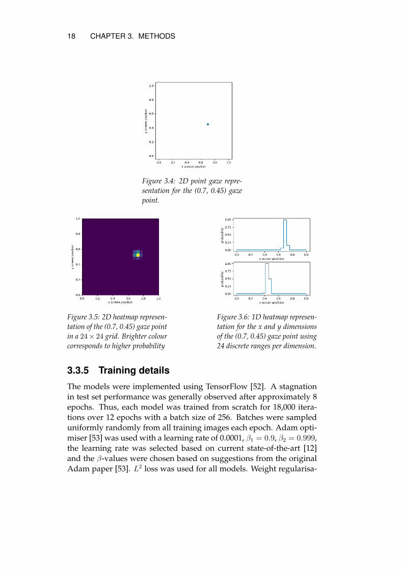
3.3.4 Ground truth labelling

The 2D point output, illustrated in Figure 3.4, used the 2D point gazeas the ground truth for the loss function. For the 2D heatmap illus-trated in Figure 3.5, the probability density function for a bivariategaussian distribution was applied to the grid and normalised to thehighest density region having density 1.0. The parameters of the bi-variate gaussian are shown in Equation 3.1. The 1D heatmaps, illus-trated in Figure 3.6, were produced in the same fashion but with sep-arate 1D gaussians for both dimensions individually with a standarddeviation of 0.0007.

µ =

[gazexgazey

], Σ =

[0.0007 0

0 0.0007

](3.1)


Figure 3.4: 2D point gaze repre-sentation for the (0.7, 0.45) gazepoint.

Figure 3.5: 2D heatmap represen-tation of the (0.7, 0.45) gaze pointin a 24× 24 grid. Brighter colourcorresponds to higher probability

Figure 3.6: 1D heatmap represen-tation for the x and y dimensionsof the (0.7, 0.45) gaze point using24 discrete ranges per dimension.

3.3.5 Training details

The models were implemented using TensorFlow [52]. A stagnationin test set performance was generally observed after approximately 8epochs. Thus, each model was trained from scratch for 18,000 itera-tions over 12 epochs with a batch size of 256. Batches were sampleduniformly randomly from all training images each epoch. Adam opti-miser [53] was used with a learning rate of 0.0001, β1 = 0.9, β2 = 0.999,the learning rate was selected based on current state-of-the-art [12]and the β-values were chosen based on suggestions from the originalAdam paper [53]. L2 loss was used for all models. Weight regularisa-


tion of 0.0005 was used similar to Krafka et al. [12] and AlexNet [10],weights were initialised as truncated normal with µ = 0, σ = 0.01 asproposed by AlexNet [10]. ReLu activation functions were used acrossthe entire network. No dropout or batch normalisation was used, sim-ilar to Krafka et al. [12] and Zhang et al. [13]. Each model was trainedand tested, both with and without calibration, 4 times. The same splitof the dataset was used between all models and all runs.

3.3.6 Calibration details

Calibration was performed using layer fine-tuning. Only the finallayer of the network was modified, except for the 2D gaze point mod-els testing calibration on several layers. Adam optimiser [53] was usedwith a learning rate of 0.000005 and all 325 of the subject’s calibrationimages were used as the single batch, and the network was trainedfor 300 iterations. The calibration was performed independently onall subjects, thus the weights were restored to pre-calibration valuesbetween each test subject. The learning rate and number of iterationswas chosen experimentally to maximise the improvement with a con-vergence fast enough to be realistic in a user calibration process. Nocross validation was used in the training due to restricted amount ofdata available for calibration. Overfitting has been observed for SVMcalibration regressors when using few gaze points [12], and expectingsimilar issues with multilayer perceptrons, all calibration points wereused as training data.

3.4 Performance metrics

Model performance was measured as the Euclidean distance error be-tween the gaze estimation and the ground truth gaze point. For theheatmap models, the gaze estimation was chosen as the centre of theregion with the highest output activation. The error of each datapointfor a model was averaged over all independent runs of the model.Model performance was compared with a baseline of average distancebetween two uniformly random points within a rectangle [54], repre-senting the model guessing uniformly random given any point. Therectangle dimensions for the baseline was the average screen size ofthe entire dataset in millimetres: 470 × 290.

Chapter 4

Results

4.1 Generic model performance

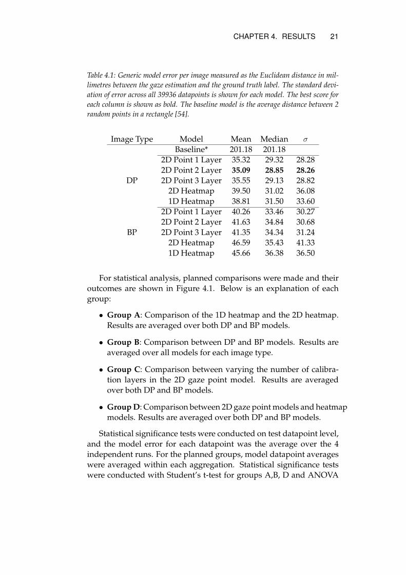
Datasets of DP and BP images were split into separate datasets andeach model was independently trained on each dataset 4 times fromscratch. Training- and test data were split on subject-level and the splitwas used for every individual run for every model for both DP and BP.The test set consisted of 168 subjects totalling 39936 data-points. Theresults on the test set for the different models without any calibrationare shown in Table 4.1. Metrics were averaged per data point overeach run and then finally averaged over each model. For example,the model producing a 2D gaze point with 2 hidden layers in the finalregressor performed, when trained and tested on DP images, a meanerror of 35.09mm, a median error of 28.85mm and the standard devi-ation of error over all averaged datapoints was 28.26mm. All modelsoutperformed the baseline and were thus considered able to infer asatisfactory estimation of the gaze.

20

CHAPTER 4. RESULTS 21

Table 4.1: Generic model error per image measured as the Euclidean distance in mil-limetres between the gaze estimation and the ground truth label. The standard devi-ation of error across all 39936 datapoints is shown for each model. The best score foreach column is shown as bold. The baseline model is the average distance between 2random points in a rectangle [54].

Image Type Model Mean Median σ

Baseline* 201.18 201.18

DP

2D Point 1 Layer 35.32 29.32 28.282D Point 2 Layer 35.09 28.85 28.262D Point 3 Layer 35.55 29.13 28.82

2D Heatmap 39.50 31.02 36.081D Heatmap 38.81 31.50 33.60

BP



For statistical analysis, planned comparisons were made and theiroutcomes are shown in Figure 4.1. Below is an explanation of eachgroup:

• Group A: Comparison of the 1D heatmap and the 2D heatmap.Results are averaged over both DP and BP models.

• Group B: Comparison between DP and BP models. Results areaveraged over all models for each image type.

• Group C: Comparison between varying the number of calibra-tion layers in the 2D gaze point model. Results are averagedover both DP and BP models.

• Group D: Comparison between 2D gaze point models and heatmapmodels. Results are averaged over both DP and BP models.

Statistical significance tests were conducted on test datapoint level,and the model error for each datapoint was the average over the 4independent runs. For the planned groups, model datapoint averageswere averaged within each aggregation. Statistical significance testswere conducted with Student’s t-test for groups A,B, D and ANOVA

22 CHAPTER 4. RESULTS

was used for testing group C. All planned comparisons resulted inrejection of the null hypothesis with p-values lower than 2 ∗ 10−5 asshown in Figure 4.1.

Figure 4.1: Depiction of the aggregations of errors within the planned groups A-Dfor the generic models. The box extends from the lower to upper quartile values ofthe data, with median shown as a vertical line in the box. The whiskers extend fromthe box show the extent of datapoints within the error range [Q1 − 1.5IQR, Q3 +

1.5IQR] where IQR is the interquartile range Q3−Q1 and Q1 and Q3 is the 25thand 75th percentile respectively.

Collectively for both DP and BP images, the heatmap models canbe seen performing worse than the 2D point approaches in Figure 4.1D.The performance difference between using 1, 2 or 3 layers for 2D pointgaze as shown in Figure 4.1C is small, post-hoc analysis of group Cwith Student’s t’test shows that differences between all pairs in groupC are statistically significant with p-values below 10−3. The collec-tive difference in performance between the 1D heatmap and the 2Dheatmap is also relatively small as seen in Figure 4.1A, though statis-


tically significant. DP models collectively performed better than BPmodels as shown in Figure 4.1B. From Table 4.1 a trend can be ob-served that suggests that DP models outperform the correspondingBP model in both mean and median performance. The DP models col-lectively also show a smaller variance in the error compared to the BPmodels as seen in Figure 4.1B.

4.2 Performance of the calibrated models

Each one of the trained generic models from Section 4.1 was evaluatedfor its performance after calibration. With the learned weights fromthe generic model, the calibration layers were trained exclusively onthe calibration data for each test subject. After the calibration training,the model performance was evaluated on the test set of the calibrationsubject. The training was performed on the generic model with fine-tuning individually for each subject. Results for the different modelswith calibration can be seen in Table 4.2. Metrics were averaged perdata point over each run and then finally averaged over each model.For example, the calibrated model producing a 2D gaze point with2 hidden layers in the regressor performed when trained and testedon DP images a mean error of 29.53mm, a median error of 22.77mmand the standard deviation of error over all averaged datapoints was27.44mm, this corresponds to a change of -5.56mm in mean and -6.08in median compared to the generic model, which are relative changesof -16% and -21% in mean and median, respectively.


Table 4.2: Calibrated model error per image measured as the Euclidean distance inin millimetres between the gaze estimation and the ground truth label. For eachcalibrated model, the change in error after calibrating the generic model, whose per-formances are shown in Table 4.1, is presented in numerical and relative differencesfor both mean and median. Relative differences are shown as percentages. A negativechange indicates model improvement. The best score for each column is shown asbold.

Image Type Model Mean Median σ Change in ErrorMean Median

Num. Rel. Num. Rel.

DP

2D Point 1 Layer 29.83 23.72 26.69 -5.27 -15 -5.60 -192D Point 2 Layer 29.53 22.77 27.44 -5.56 -16 -6.08 -212D Point 3 Layer 34.75 25.22 27.96 -0.80 -2.2 -3.91 -13

2D Heatmap 49.29 30.42 69.85 +9.21 +23 -0.60 -1.91D Heatmap 51.99 37.75 51.77 +13.18 +34 +6.25 +20

BP

2D Point 1 Layer 33.73 27.23 27.61 -6.53 -16 -6.23 -192D Point 2 Layer 34.79 27.44 29.60 -6.48 -16 -7.4 -212D Point 3 Layer 36.40 29.49 29.63 -4.95 -12 -4.85 -14

2D Heatmap 64.47 34.83 87.96 +18.9 +39 -0.60 -1.71D Heatmap 48.76 37.45 42.51 +3.10 +6.7 +1.07 +2.9

The mean error of each test subject before and after calibration weretested for significance using the Wilcoxon signed-rank test on the pop-ulation of test datapoints for each model. All statistical tests rejectedthe null hypothesis with p-values smaller than 10−16. The plannedgroups presented in Section 4.1 were used and statistical analysis wasconducted on each group as outlined in Section 4.1. The results for thegroups are displayed in Figure 4.2. The tests showed statistical signif-icance for all groups A–D with p-values smaller than 10−16.


Figure 4.2: Depiction of the aggregations of errors within the planned groups definedin Section 4.1 as A-D for the calibrated models. The box extends from the lowerto upper quartile values of the data, with median shown as a vertical line in the box.The whiskers extend from the box show the extent of datapoints within the error range[Q1 − 1.5 ∗ IQR,Q3 + 1.5 ∗ IQR] where IQR is the interquartile range Q3 −Q1

and Q1 and Q3 is the 25th and 75th percentile respectively.

From the results in Figure 4.2D, it is shown that the calibrated 2Dpoint models collectively outperform the calibrated heatmap models.Looking at Figure 4.2B, DP models continue to collectively outperformBP models after calibration. From Figure 4.2C it is observed that the 3layer calibration performs slightly worse than 1 or 2 calibration layermodels, the differences between all pairs in comparison C were shownstatistically significant in post hoc analysis with p-values smaller than10−8. The calibrated 1D heatmap models collectively show better me-dian performance but larger variance compared to the calibrated 2Dheatmap models as seen in Figure 4.2A.

For the evaluation of calibration effect, two additional planned groups


were introduced:

• Group E: Comparison of the generic- and calibrated 2D pointmodels. Results are averaged over both DP and BP models.

• Group F: Comparison of the generic- and calibrated heatmapmodels. Results are averaged over both DP and BP models

Statistical significance tests were conducted with Student’s t-testfor both groups E and F over the averaged data points over each modelwithin each group. The planed comparisons for groups E and F re-sulted in rejection of the null hypothesis with p-values lower than10−16 as shown in Figure 4.3.

Figure 4.3: Depiction of the aggregations of errors within the planned groups E and Fshowing, displaying the effect of calibration. The box extends from the lower to upperquartile values of the data, with median shown as a vertical line in the box. Thewhiskers extend from the box show the extent of datapoints within the error range[Q1 − 1.5 ∗ IQR,Q3 + 1.5 ∗ IQR] where IQR is the interquartile range Q3 −Q1

and Q1 and Q3 is the 25th and 75th percentile respectively.

In Figure 4.3 the effect of calibration for groups E and F can beobserved. The calibrated 2D point models are shown in Figure 4.3Eperforming collectively better than the generic models. In contrast,the calibrated heatmap models performs collectively worse than thegeneric models as shown in Figure 4.3F.

The results show that calibration using transfer learning can in-crease the performance of the gaze estimation for 2D point modelswith an average of 15%, up to 21% as seen in Table 4.2. However, itis also shown that transfer learning calibration can cause performance


to drastically decrease in other output presentations. Calibrating us-ing transfer learning consistently shows improvement for the 2D gazeoutput in all models independently of image type and number of cal-ibration layers, but conversely shows the same consistency in reduc-ing performance in the 1D- and 2D heatmap models. This suggeststhat transfer learning consistently can improve gaze estimation per-formance of current state-of-the-art models, but that the method doesnot successfully transfer to all deep CNN-based gaze estimation archi-tectures.

4.3 Training exclusively on calibration data

By applying transfer learning onto a generic model in order to max-imise the performance of a single test subject it is assumed that thepre-training step is a necessary component prior to training the modelon the calibration data of the subject. This assumption was testedby training the models on a single test subject’s calibration data fromscratch and evaluating the model on that single subject’s test data. Thiswas done for all test subjects on all models. The results are presentedin Table 4.3. Metrics were averaged per data point over each modeltrained and evaluated on a single subject. For example, The modelproducing a 2D gaze point with 3 hidden layers in the final regressorperformed, when trained and tested on DP images, a mean error of96.28mm, a median error of 83.87mm and the standard deviation oferror over all averaged data points was 57.57mm.

All models, except the 2D DP heatmap model, performed betterthan the baseline and were thus considered able to infer an estimationof the gaze. However, the performance can be observed, as expected,to perform magnitudes worse than the calibrated transfer learningresults shown in Table 4.2. The average datapoint errors of all cali-brated models and the average datapoint errors of the calibration-onlytrained models were compared with the Wilcoxon signed-rank test re-sulting in rejection of the null hypothesis with a p-value smaller than10−16. This result strongly suggests that the calibrated performance ob-served in the transfer learning model is not achievable on subject-leveltraining from scratch with only the calibration data.


Table 4.3: Average model error per image for models trained on a single subject’scalibration data and evaluated on the subject’s test data. Error is measured as theEuclidean distance in millimetres between the gaze estimation and the ground truthlabel. The best score for each column is shown as bold. The baseline model is theaverage distance between 2 random points in a rectangle [54].

Image Type Model Mean Median σ

Baseline* 201.18 201.18

DP



BP



4.4 Calibration transformations

In Figures 4.4, 4.5, and 4.6 the range of complexity for calibration trans-formation using different amount of layers in the final parts of the 2Dgaze point model are shown. For 2D gaze point inference, calibrationshows transformations similar to vector fields. Proximity between thepositions of non-calibrated gaze estimations correlates with similari-ties in offset. An overall transformation shape can be observed foreach subject in all models. As seen in Figure 4.4, a single layer cali-bration applies uniform transformations where most gaze points havea similar transformation. The direction shows some moderate vari-ance, but the magnitude shows more variance. Increasing the numberof calibration layers to 2, as shown in Figure 4.5, increases the vari-ation in the transformation directions, prominent swirl patterns be-comes more common. Magnitude range still remains broad. Figure 4.6shows transformations for calibration with 3 layers, while these trans-formations are similar to that achieved with 2 calibration layers, spatialindependence is stronger and transformations appear more local. Anoverall transformation shape is still visible, but more complex.


Simple linear shifts, or slight nudges appear for all 3 model vari-ations. Thus, more layers does not implicate more complex transfor-mations for all subjects. Figures 4.4, 4.5, 4.6 only show complexitypotential for the calibration models. Given that the 3 layer calibra-tion yielded less improvement compared to 1 or 2 calibration layersas shown in Table 4.2, it is assumed that the complex transformationsof the 3 layer calibration becomes too specific and overfits for the 9calibration data-points.

Figure 4.4: Two representative samples of calibration transformations with 1 hiddenlayer for 2D gaze points inference. Gaze points estimated by the generic model areshown as circles, the estimations from the calibrated model are shown as dots. Linesconnects the estimations of the generic- and calibrated model for each datapoint.


Figure 4.5: Two representative samples of calibration transformations with 2 hiddenlayers for 2D gaze points inference. Gaze points estimated by the generic model areshown as circles, the estimations from the calibrated model are shown as dots. Linesconnects the estimations of the generic- and calibrated model for each datapoint.

Figure 4.6: Two representative samples of calibration transformations with 3 hiddenlayers for 2D gaze points inference. Gaze points estimated by the generic model areshown as circles, the estimations from the calibrated model are shown as dots. Linesconnects the estimations of the generic- and calibrated model for each datapoint.

Chapter 5

Discussion

5.1 Key findings

Improvements in median performance for the best performing cali-brated 2D point models were observed in a range of 15% to 21%, whichis in line with the performance improvement of 16% and 22% observedfor the SVM calibration proposed by Krafka et al. [12]. This suggeststhat both calibration approaches perform similarly and indicates thatintroducing SVMs for the purpose of calibration is excessive for eyetracking in deep CNN-based appearance based models. Additionally,in the calibration procedure by Krafka et al. 13 calibration points wereused as opposed to 9 calibration points used in this thesis. Therefore,due to differences in datasets and training data, suggestions for futurework include comparing the improvement in performance from trans-fer learning and the SVM calibration method, proposed by Krafka etal. [12], on the same dataset for a reliable comparison.

The results demonstrate that more complex output representationssuch as the probabilistic heatmap models are able to estimate gazewith slightly worse performance than the traditional 2D point outputrepresentation in generic models. The architectures of the heatmapmodels were not explored thoroughly and could be explored furtherin future work. Probabilistic gaze models could provide new means ofinterfacing with eye tracking technology, e.g. providing the probabil-ity that a given screen object is looked upon. Previous work in the fieldhas examined a narrow set of output representations for gaze estima-tion, and the results of this thesis suggests that other types of outputrepresentations could perform well and extend the possibilities of the

31

32 CHAPTER 5. DISCUSSION

eye tracking interfaces.This thesis has shown that model performance can be drastically

improved using the principles of transfer learning. By treating sub-jects as individual domains within the dataset, the network can bepre-trained on a large dataset consisting of other subjects and then canbe fine-tuned on the subject data, previously unseen, resulting in im-proved performance compared to the generic model. Thus, a methodfor calibrating a generic model to specialise on a narrow subset of itsdata space has been motivated. However, future work should investi-gate if a generic model trained on a specific dataset of gaze-annotatedface images can be successfully calibrated for a subject from a distinc-tively different dataset of gaze-annotated face images. This is expectedto produce satisfactory results based on previous research in transferlearning.

5.2 Limitations

The tests in this thesis were performed on a single dataset that hasnot been used in any previous publications resulting in inability tomake direct comparisons with the results of other previous studies.The models used in this thesis were inspired by models used for full-face images [12, 13], whereas the dataset used in this thesis consisted ofROI images. This introduces variation that cannot be accounted for ina direct comparison. However, the results of this study are in line withresults of current state-of-the-art [12] and it is expected that the modelswould perform similarly with another large-scale dataset consisting ofa different type of gaze annotated images.

Significant differences were observed between the 2D gaze pointmodels and the heatmap models. However, the heatmap models werenot explored thoroughly and from the results a conclusion that theoutput representations performs strictly worse than the 2D gaze pointmodels cannot be justified, although it is suggested. The heatmapmodels have more complex output and the observed worse perfor-mance could be a manifestation of a model that is harder to train andmore sensitive to hyperparameter values. Future work could exploreif generic heatmap model performance can be improved.

The calibration training process used the same hyperparametersacross all models. Hyperparameter choice was not trivial as a large

CHAPTER 5. DISCUSSION 33

variation was observed both between individual subjects and differentmodels. Although the selection of hyperparameters was made from asmall pool of choices, performance increase due to calibration is ex-pected to be further improved by optimising hyperparameter settingsfor individual models.

The results showed a high variance in error, especially for largererrors. The thesis assumes that the dataset is mostly correct and thatthe subjects look at the gaze point shown in the screen. However,analysing a subset of the images with bad performance shows thatthe dataset consists of varying quality, e.g. in some images, the sub-ject is looking at the wrong part of the screen or looking away. Nofiltering was performed on the dataset due to its scale, which proba-bly introduced noise into both the training- and test set. Although nomajor improvement is expected, having less noise in the data could beattempted.

Additional metadata such as head pose information as input to theregression models has been used in previous research. Given that adataset with multiple screen sizes was used for this thesis, this couldhave introduced noise since the gaze position output was relative. Nei-ther head pose data or screen size information was input to the modelsin this thesis. However, it is expected that inclusion of screen size asan input could improve the performance of the models since the phys-ical output space represented by the gaze output is dependent on thescreen size.

5.3 Ethics and sustainability

One of the main ethical concerns of data driven models with data orig-inating from human individuals is the risk of introducing bias out ofignorance or intent. Training generic models need to test for a widerange of people as possible in order to avoid discrimination of pos-sible users. This distinction is not limited to only ethnic groups butincludes, for eye tracking, usage of glasses, scars, and other prominentfeatures of the face. While it is not expected for a generic model to per-form evenly across any artificial grouping of people, making an effortto identify a possible lack of representation in the test data and con-sidering model performance for distinct sub-groups in relation to theperformance of the entire set is to take ethical considerations seriously.

34 CHAPTER 5. DISCUSSION

As in all of machine learning and data science, the production of-and utilisation of more data is self-motivated. Although eye trackingcurrently does not see the same scale of big data as in other fields,finding ways to utilise all available data provides sustainability by re-cycling data, making the production of said data more efficient, morevaluable, and possible reduces the need of data production. This is es-pecially relevant when the production of new data is expensive. In thisthesis, data from two different camera models were joined into a singledataset performing better than its parts. If deep CNN-models gener-alise variations within a domain without loss in performance, need forproducing new data can be drastically reduced since the majority ofthe data need can be obtained by data recycling.

Deep learning systems are usually deployed on external serversclusters, separating the networks from the host system. This providescomputation power, flexibility and security. The main downside isthat feedback quality becomes dependant on network traffic delays.In real-time systems, running ANN systems on external servers intro-duces risk in accessibility and quality of experience. However, host-based systems with trained ANN introduce security risks, with directaccess to the ANN, it is exposed and the confidentiality of the datacould be threatened since information about the data used for trainingcan be extracted. This could be of ethical concern depending on thetype of data that is used to train the system, especially if it originatesfrom human individuals. Running real-time systems with host ANNcomponents need to consider the confidentiality of the data and theethical risks involved in exposing a trained ANN system.

Chapter 6

Conclusion

The results show that individual user calibration using transfer learn-ing can consistently improve the performance of 2D point gaze esti-mation in appearance-based models for eye tracking. The best im-proving models show improvements of up to 21% in median error,which is in line with the calibration results of the current state-of-the-art. It is shown that the fine-tuning of several layers, instead ofsingle layer fine-tuning, does not necessarily further improve the per-formance over the generic models. It is noted that transfer learningcalibration does not improve the performance of heatmap-based gazeoutput representations, suggesting that transfer learning does not im-prove the performance for all ANN architectures for gaze estimation.In conclusion, calibration exploiting transfer learning offers promisingperformance. However, it is emphasised that the proposed calibrationmethod is not fully optimised and could be improved in future work.

35

Bibliography

[1] Dan Witzner Hansen and Qiang Ji. “In the eye of the beholder:A survey of models for eyes and gaze”. In: IEEE transactions onpattern analysis and machine intelligence 32.3 (2010), pp. 478–500.

[2] Michel Wedel and Rik Pieters. “A review of eye-tracking researchin marketing”. In: Review of marketing research. Emerald GroupPublishing Limited, 2008, pp. 123–147.

[3] Alex Poole and Linden J Ball. “Eye tracking in HCI and usabilityresearch”. In: Encyclopedia of human computer interaction 1 (2006),pp. 211–219.

[4] Laura A. Granka, Thorsten Joachims, and Geri Gay. “Eye-trackingAnalysis of User Behavior in WWW Search”. In: Proceedings of the27th Annual International ACM SIGIR Conference on Research andDevelopment in Information Retrieval. SIGIR ’04. Sheffield, UnitedKingdom, 2004, pp. 478–479. ISBN: 1-58113-881-4.

[5] Peter M Corcoran et al. “Real-time eye gaze tracking for gamingdesign and consumer electronics systems”. In: IEEE Transactionson Consumer Electronics 58.2 (2012).

[6] Päivi Majaranta and Kari-Jouko Räihä. “Twenty years of eye typ-ing: systems and design issues”. In: Proceedings of the 2002 sym-posium on Eye tracking research & applications. ACM. 2002, pp. 15–22.

[7] Andrew T Duchowski. “A breadth-first survey of eye-trackingapplications”. In: Behavior Research Methods, Instruments, & Com-puters 34.4 (2002), pp. 455–470.

[8] Elias Daniel Guestrin and Moshe Eizenman. “General theory ofremote gaze estimation using the pupil center and corneal reflec-tions”. In: IEEE Transactions on biomedical engineering 53.6 (2006),pp. 1124–1133.

36

BIBLIOGRAPHY 37

[9] Yusuke Sugano, Yasuyuki Matsushita, and Yoichi Sato. “Learning-by-synthesis for appearance-based 3d gaze estimation”. In: Pro-ceedings of the IEEE Conference on Computer Vision and Pattern Recog-nition. 2014, pp. 1821–1828.

[10] Alex Krizhevsky, Ilya Sutskever, and Geoffrey E Hinton. “Im-agenet classification with deep convolutional neural networks”.In: Advances in neural information processing systems. 2012, pp. 1097–1105.

[11] Xucong Zhang et al. “Appearance-based gaze estimation in thewild”. In: Proceedings of the IEEE Conference on Computer Visionand Pattern Recognition. 2015, pp. 4511–4520.

[12] Kyle Krafka et al. “Eye Tracking for Everyone”. In: IEEE Confer-ence on Computer Vision and Pattern Recognition (CVPR). 2016.

[13] Xucong Zhang et al. “It’s Written All Over Your Face: Full-FaceAppearance-Based Gaze Estimation”. In: arXiv preprint arXiv:1611.08860(2016).

[14] Yafei Wang et al. “Appearance-based gaze estimation using deepfeatures and random forest regression”. In: Knowledge-Based Sys-tems 110 (2016), pp. 293–301.

[15] Kar-Han Tan, David J Kriegman, and Narendra Ahuja. “Appearance-based eye gaze estimation”. In: Applications of Computer Vision,2002.(WACV 2002). Proceedings. Sixth IEEE Workshop on. IEEE.2002, pp. 191–195.

[16] Zoltán Tosér et al. “Personalization of Gaze Direction Estima-tion with Deep Learning”. In: KI 2016: Advances in Artificial In-telligence: 39th Annual German Conference on AI, Klagenfurt, Aus-tria, September 26-30, 2016, Proceedings. Ed. by Gerhard Friedrich,Malte Helmert, and Franz Wotawa. Cham: Springer InternationalPublishing, 2016, pp. 200–207. ISBN: 978-3-319-46073-4. DOI: 10.1007/978-3-319-46073-4_20.

[17] Sinno Jialin Pan and Qiang Yang. “A survey on transfer learn-ing”. In: IEEE Transactions on knowledge and data engineering 22.10(2010), pp. 1345–1359.

[18] Dumitru Erhan et al. “Why does unsupervised pre-training helpdeep learning?” In: Journal of Machine Learning Research 11.Feb(2010), pp. 625–660.

38 BIBLIOGRAPHY

[19] Karen Simonyan and Andrew Zisserman. “Very deep convo-lutional networks for large-scale image recognition”. In: arXivpreprint arXiv:1409.1556 (2014).

[20] Jonathan Long, Evan Shelhamer, and Trevor Darrell. “Fully con-volutional networks for semantic segmentation”. In: Proceedingsof the IEEE Conference on Computer Vision and Pattern Recognition.2015, pp. 3431–3440.

[21] Carlos Hitoshi Morimoto et al. “Pupil detection and tracking us-ing multiple light sources”. In: Image and vision computing 18.4(2000), pp. 331–335.

[22] Ian Goodfellow, Yoshua Bengio, and Aaron Courville. Deep Learn-ing. http://www.deeplearningbook.org. MIT Press, 2016.

[23] Yoshua Bengio et al. “Deep learning of representations for un-supervised and transfer learning.” In: ICML Unsupervised andTransfer Learning 27 (2012), pp. 17–36.

[24] Jia Deng et al. “Imagenet: A large-scale hierarchical image database”.In: Computer Vision and Pattern Recognition, 2009. CVPR 2009. IEEEConference on. IEEE. 2009, pp. 248–255.

[25] Matthew D Zeiler and Rob Fergus. “Visualizing and understand-ing convolutional networks”. In: European conference on computervision. Springer. 2014, pp. 818–833.

[26] Christopher D. McMurrough et al. “An Eye Tracking Dataset forPoint of Gaze Detection”. In: Proceedings of the Symposium on EyeTracking Research and Applications. ETRA ’12. Santa Barbara, Cal-ifornia, 2012, pp. 305–308. ISBN: 978-1-4503-1221-9.

[27] U Weidenbacher et al. “A comprehensive head pose and gazedatabase”. In: (2007).

[28] Brian A. Smith et al. “Gaze Locking: Passive Eye Contact De-tection for Human-object Interaction”. In: Proceedings of the 26thAnnual ACM Symposium on User Interface Software and Technol-ogy. UIST ’13. St. Andrews, Scotland, United Kingdom, 2013,pp. 271–280. ISBN: 978-1-4503-2268-3.

BIBLIOGRAPHY 39

[29] Kenneth Alberto Funes Mora, Florent Monay, and Jean-MarcOdobez. “EYEDIAP: A Database for the Development and Eval-uation of Gaze Estimation Algorithms from RGB and RGB-DCameras”. In: Proceedings of the Symposium on Eye Tracking Re-search and Applications. ETRA ’14. Safety Harbor, Florida, 2014,pp. 255–258. ISBN: 978-1-4503-2751-0.

[30] Yusuke Sugano, Yasuyuki Matsushita, and Yoichi Sato. “Learning-by-Synthesis for Appearance-based 3D Gaze Estimation”. In: TheIEEE Conference on Computer Vision and Pattern Recognition (CVPR).2014.

[31] Qiong Huang, Ashok Veeraraghavan, and Ashutosh Sabharwal.“TabletGaze: unconstrained appearance-based gaze estimationin mobile tablets”. In: arXiv preprint arXiv:1508.01244 (2015).

[32] Yusuke Sugano et al. “An incremental learning method for un-constrained gaze estimation”. In: European Conference on Com-puter Vision. Springer. 2008, pp. 656–667.

[33] Feng Lu et al. “A head pose-free approach for appearance-basedgaze estimation.” In: BMVC. 2011, pp. 1–11.

[34] Feng Lu et al. “Head pose-free appearance-based gaze sensingvia eye image synthesis”. In: Pattern Recognition (ICPR), 2012 21stInternational Conference on. IEEE. 2012, pp. 1008–1011.

[35] Xiying Wang et al. “Hierarchical gaze estimation based on adap-tive feature learning”. In: Image Processing (ICIP), 2014 IEEE In-ternational Conference on. IEEE. 2014, pp. 3347–3351.

[36] Kenneth Alberto Funes Mora and Jean-Marc Odobez. “Gaze es-timation from multimodal kinect data”. In: Computer Vision andPattern Recognition Workshops (CVPRW), 2012 IEEE Computer So-ciety Conference on. IEEE. 2012, pp. 25–30.

[37] Feng Lu et al. “Learning gaze biases with head motion for headpose-free gaze estimation”. In: Image and Vision Computing 32.3(2014), pp. 169–179.

[38] Yann LeCun, Corinna Cortes, and Christopher JC Burges. TheMNIST database of handwritten digits. 1998.

[39] J. Deng et al. “ImageNet: A Large-Scale Hierarchical Image Database”.In: CVPR09. 2009.

40 BIBLIOGRAPHY

[40] Kenneth Alberto Funes Mora and Jean-Marc Odobez. “Personindependent 3d gaze estimation from remote rgb-d cameras”.In: Image Processing (ICIP), 2013 20th IEEE International Conferenceon. IEEE. 2013, pp. 2787–2791.

[41] Erroll Wood and Andreas Bulling. “Eyetab: Model-based gazeestimation on unmodified tablet computers”. In: Proceedings ofthe Symposium on Eye Tracking Research and Applications. ACM.2014, pp. 207–210.

[42] Chih-Chuan Lai et al. “Appearance-based gaze tracking withfree head movement”. In: Pattern Recognition (ICPR), 2014 22ndInternational Conference on. IEEE. 2014, pp. 1869–1873.

[43] Li-Qun Xu, Dave Machin, and Phil Sheppard. “A Novel Ap-proach to Real-time Non-intrusive Gaze Finding.” In: BMVC.1998, pp. 1–10.

[44] Feng Lu and Xiaowu Chen. “Person-independent eye gaze pre-diction from eye images using patch-based features”. In: Neuro-computing 182 (2016), pp. 10–17.

[45] Shumeet Baluja and Dean Pomerleau. “Non-intrusive gaze track-ing using artificial neural networks”. In: (1994).

[46] Feng Lu et al. “Adaptive linear regression for appearance-basedgaze estimation”. In: IEEE Transactions on Pattern Analysis andMachine Intelligence 36.10 (2014), pp. 2033–2046.

[47] Weston Sewell and Oleg Komogortsev. “Real-time Eye Gaze Track-ing with an Unmodified Commodity Webcam Employing a Neu-ral Network”. In: CHI ’10 Extended Abstracts on Human Factorsin Computing Systems. CHI EA ’10. Atlanta, Georgia, USA, 2010,pp. 3739–3744. ISBN: 978-1-60558-930-5.

[48] Yann LeCun et al. “Gradient-based learning applied to docu-ment recognition”. In: Proceedings of the IEEE 86.11 (1998), pp. 2278–2324.

[49] Yi Sun et al. “Deep learning face representation by joint identification-verification”. In: Advances in neural information processing systems.2014, pp. 1988–1996.

[50] Jonathan Tompson et al. “Efficient object localization using con-volutional networks”. In: Proceedings of the IEEE Conference onComputer Vision and Pattern Recognition. 2015, pp. 648–656.

BIBLIOGRAPHY 41

[51] Ali M Reza. “Realization of the contrast limited adaptive his-togram equalization (CLAHE) for real-time image enhancement”.In: The Journal of VLSI Signal Processing 38.1 (2004), pp. 35–44.

[52] Martín Abadi et al. “Tensorflow: Large-scale machine learningon heterogeneous distributed systems”. In: arXiv preprint arXiv:1603.04467(2016).

[53] Diederik Kingma and Jimmy Ba. “Adam: A method for stochas-tic optimization”. In: arXiv preprint arXiv:1412.6980 (2014).

[54] AM Mathai, P Moschopoulos, and G Pederzoli. “Random pointsassociated with rectangles”. In: Rendiconti del Circolo Matematicodi Palermo 48.1 (1999), pp. 163–190.

www.kth.se

Documents

Calibration in Eye Tracking Using Transfer Learningann/exjobb/david_masko.pdfDEGREE PROJECT IN COMPUTER SCIENCE AND ENGINEERING, SECOND CYCLE, 30 CREDITS STOCKHOLM, SWEDEN 2017 Calibration