CALIBRATION OF A WHOLE OF WORKS PROCESS SIMULATION MODEL FOR THE MANGERE WASTEWATER TREATMENT PLANT

Kevan Brian, AWT New Zealand Peter Trafford, Watercare Services Limited

ABSTRACT The Mangere Wastewater Treatment Plant (WWTP), situated on the Manukau Harbour, receives the wastewater flow from four municipalities of greater Auckland, treating a population equivalent of one million. The design average inflow to the plant is 390,000 m³/day and the current load to the plant consists of 120 tonnes/day of BOD5, 130 tonnes/day of total suspended solids (TSS), 18 tonnes/day of total nitrogen (TN), and 1.8 tonnes/day of total phosphorous (TP). This large plant provides primary, secondary and advanced level treatment for all flows up to 9 m3/s and primary treatment and UV disinfection for further storm flows of 9 - 16.5 m 3/s. The plant is designed to achieve an effluent standard of 15 mg/L TBOD5, 15 mg/L TSS and a total nitrogen of 9.5 mg/L (summer) and 35 mg/L (winter).

A “whole of works” BioWin model was calibrated using the protocols and suggested analytical testing contained in “Methods for Wastewater Characterization in Activated Sludge Modeling”, WERF 2003.

This paper presents a summary of the testing results versus model for each unit process and a discussion of the SBR protocol and its application to a complex treatment process such as Mangere. The paper also discusses some of the key factors influencing the model calibration and some o f the difficulties and uncertainties associated with collection, measurement and interpretation of analytical and SBR data for model calibration.

KEYWORDS Process Simulation, calibration, uncertainty, SBR protocol

1 INTRODUCTION

The Mangere WWTP is the largest wastewater treatment facility in New Zealand with a population equivalent of approximately 1 million people (see figure1). It discharges, on average, 300,000 cubic metres of treated wastewater into the Manukau Harbour per day.

The treatment process consists of a number of u nit operations including:

• Screening and grit removal

• Primary sedimentation

• Secondary biological treatment via activated sludge

• Tertiary filtration and UV disinfection

• Solids thickening, digestion and dewatering

Figure 1: Aerial View of the Mangere WWTP

In order to understand the interrelationships between each unit process, the effect of effluent q uality, solids production and operational cost, a process simulation model was built using BioWin simulation software. Details of the model build can be found in McCoy et al 2007.

BioWin simulation software provides a platform f or the simulation of wastewater treatment processes via modified Activated Sludge Models (ASM) and an Anaerobic Digestion Model (AD).

The BioWin AS/AD model uses ASM variables and a digestion model that is based upon these variables. The key to these models is the “state variables” which make up the basis of the model predictions. The state variables include parameters that cannot be broken down into sub groups such as ammonia, reactor temperature, etc.

The AS/AD model is based on a Chemical Oxygen Demand, Nitrogen and Phosphorus mass balance. Each of these components is broken down in the model to a state variable. For example COD is broken down as shown in Figure 2:

Figure 2: Breakdown of COD fractions in BioWin

Calibration of the AS/AD model therefore includes measuring and estimating the wastewater “fractions” and in some instances measurement and modification of kinetic and sto ichiometric parameters.

Total COD

(CODt)

Unbiodegradable COD Biomass

(Xb) Biodeg radable

COD

Soluble (fus)

Slowly Deg radable (Xsc + Xsp)

Readily Deg radable

(fbs) Particulate (fup)

Measurement of the wastewater fractions and their application to the model can be complex and typically involves a range of standard and specialized laboratory tests. Guidelines for this testing have been developed over a number of case studies and research programs and are summarized in “Methods for Wastewater Characterization in Activated Sludge Modeling” published by the Water Environment Federation (WEF).

A general guideline for creating a calibrated model based on these methods is summarized in Figure 3 below.

Figure 3: Modelling Approach

The above approach was used as the basis for the calibration of the Watercare “whole plant” model (note that a “whole plant” model refers to the integrated modeling of all the main unit processes in an integrated simulation package, and can also be referred to as a “super” model).

This paper summarizes the techniques used to calibrate the Mangere model, provides a comparison of modelled versus measured data and an analysis of the challenges of integrating this information into a simulation.

2 METHODS

2.1 ANALYTICAL METHODS The first stage of the model calibration was to identify the critical streams around the process and to develop a sampling program and pro tocol for each stream. As the Mangere plant has a large number of recycles and interdependent process streams, identification of the sample location and sample type was critical to the success of the calibration. A sampling program was developed that identified nine sample points around the process along with 28 points where flow measurements were recorded on the site SCADA or could be determined by calculation. Sample parameters are summarized in Table 1 below. Ten samples were taken at each of the nine sample points identified above.

Identification of key parameters

Mass Balance

WWTP Analyses and measurement

Mass Balance

Bench-top Analysis

Development of initial model

Calibration using mass balances

Final Calibrated Model

Table 1: Analytical Samples

Parameter Short Sample Name Sample Frequency

Chemical Oxygen Demand CODt (total COD)

CODt Daily

Filtered COD (125 micron) CODf Daily

Filtered and Flocculated COD (modified UCT method)

CODff Daily

Carbonaceous BOD5 BOD Daily

Filtered Carbonaceous BOD5 BODs Daily

Total Suspended Solids (125 micron) TSS Daily

Volatile Suspended Solids VSS Daily

Total Kiedhal nitrogen TKN Daily

Filtered TKN (125 micron) TKNs Daily

Ammonia NH4-N Daily

Nitrate NO3-N Daily

Total Phosphorus TP Daily

Dissolved Reactive Phosphorus DRP Daily

pH - Daily

Flow - Daily

2.2 BENCH SCALE SBR The limitation of the analytical methods for the fractionation of the COD components is the measurement of the unbiodegradable particulate COD fraction (Sup in Biowin or Xi in ASM models). The Sup fraction of the COD is very important for predictions of mixed liquor concentration, waste solids mass and the performance of anaerobic digesters. Using Mangere as an example, the over estimation of Sup by 25% would increase the solids inventory in the model by 20,000kgDS/d.

The best way to minimize the error in the estimation of the Sup concentration is to use a bench scale reactor. This enables a complete mass balance to be undertaken across the reactor under controlled loading and SRT conditions. A balance over the influent, waste solids and final effluent allows the Sup concentration to be fitted to the reactor data by means of a total COD balance. This balance can also be verified by modelling the bench scale system in BioWin.

One of the disadvantages of the SBR protocol is that the reactor cannot be run on all the wastewater streams at the same time. Hence one stream has to be identified for the SBR and the other streams that combine to make this stream evaluated by difference. At Mangere the interstage pump station (IPS) that feeds the nine reactor clarifiers was selected for the SBR trial. This is because the IPS:

• Receives primary treated wastewater that includes all recycles.

• Feeds the biological treatment stage (this has the longest solids retention time of any unit process).

• The composition of the WAS generated from the IPS flow determines the solids flux to secondary sludge thickening.

• The prediction of the reactor clarifier mixed liquor is most sensitive to the Sup concentration.

The influent feed to the SBR was taken from a 24 hour composite sample of the IPS. In order to ensure representative sampling, composite weekend samples were also included. The IPS wastewater sub-samples were combined and tested for COD. To achieve controlled reactor conditions the inlet COD concentration to the SBR must be maintained as constant as possible. This was achieved by diluting the raw composite samples to 400mgCOD/L with tap water. Each day, the SBR was fed a total of 4 litres of diluted wastewater. Baking soda (NaHCO3) was also added to increase the alkalinity of the feed and raise the pH to above 7 in the decant. This was calculated based on the concentration of ammonia within the diluted wastewater and was around 250 mg per day.

2.2.1 SBR CYCLES The cycles for the SBR were as follows:

• Fill 09:00 4 litres of diluted wastewater was pumped into the SBR;

• Aeration 09:20 Following end of feed period, aeration and mixing was begun and this react phase ran for 23 hours;

• Wasting 07:45 Approximately 270 mL of mixed liquor was manually wasted;

• Settling 08:00 Aeration and mixing were stopped and the system allowed to settle for 30 minutes;

• Decant 08:30 Following the settling of the system 4 litres was decanted from the reactor.

No denitrification phase was includ ed in the SBR schedule. For calculation of the fractions required for the BioWin calibration denitrification was not required as the fractions are wastewater specific not process specific.

3 RESULTS AND ANALYSIS

3.1 ANALYTICAL TESTING To characterize the influent wastewater, the COD fractions were determined using the following method (based on WERF Manual “Methods for Wastewater Characterization in Activated Sludge Modelling” and STOWA).

3.1.1 COD FRACTIONS 1. Measurement of the CODt (total COD), fCOD (filtered COD) and ff COD (filtered and flocculated COD)

concentrations.

2. Measurement of the ffCOD concentration in the effluent. The concentration of ffCOD in the effluent (plant discharge) is equivalent to the soluble, unbiodegradable concentration, SUS. The fUS fraction is the SUS / CODt.

3. The difference between the influent ffCOD and SUS (determined as above) is the soluble biodegradable concentration SBS. The fBS fraction is the SBS / CODt.

4. The colloidal COD fraction (XSC) is represented by the difference between the fCOD and the ffCOD concentrations.

5. The particulate concentrations are more difficult to determine. The User Manual for BioWin 2.1 (EnviroSim 1991) contains a section to calculate the BOD values associated with the soluble and particulate COD concentrations based on the slowly biodegradable particulate concentration XSP as follows:

( ) ( ) ( )tbSSS eSYfSYBOD .1(...1.1 −−−+−= (1)

( ) ( )( ) ( ) ( )

( ) ( )

−

−−

−

−

−−

+−= −− tbtkSPSP e

kbkYf

ekb

YbfYXBOD .. 1.

.).11.

..11. (2)

Where:

Y = Yield of active organisms (~ 0.666 mg cell COD/mgCOD)

SS = Soluble (filtered) biodegradable COD (mgCOD/L) – includes colloidal

f = fraction of active mass remaining as endogenous residue (~0.20)

b = Endogenous decay rate constant (~ 0.24 d-1)

k = first order rate constant for sb COD degradation (~0.40 d-1)

t = time (d)

Comparisons were made between the measured total BOD and filtered BOD and their calculated equivalents. The XSP value was iterated to provide comparab le BOD values.

6. The inert particulate fraction, fUP, is also difficult to analytically quantify. However, by definition:

( )CODt

XXfff SPSC

USBSUP+

−−−= 1 (3)

As fBS and f US have been calculated, XSC and the CODt measured, and XSP estimated, fUP can be calculated.

7. The last ‘fraction’ to be calculated is the amount of non-colloidal slowly biodegradable COD that is particulate.

SPSC

SPXSP XX

Xf

+= (4)

The major assumption in using this method is that while the fUS and f BS fractions are measured variables the fUP is calculated based on the particulate BOD (i.e. the Xsp concentration and the measured particulate BOD). Hence there is some error associated with this method as the BOD test if difficult to replicate and model accurately. The other assumption that has been made is that particulate COD that is degradable does not include biomass COD.

3.1.2 NITROGEN FRACTIONS The nitrogen fractions that were calculated were:

1. fNA TKN to ammonia ratio:

[ ][ ]TKNNH

f NA

+

= 4 (5)

2. fNOX Fraction of organic nitrogen that is particulate –

[ ] [ ]( ) [ ] [ ]( )[ ] [ ]( )+

++

−−−−

=4

44

NHTKNNHTKNfNHTKN

f NOX (6)

The SBR was operated for approximately three sludge ages (62days) in order to obtain “steady state” conditions. Following this a 10 day intensive sampling period was undertaken including samples for TSS; VSS; filtered COD; filtered and flocculated COD; filtered TKN; TKN; and TN. In addition, further testing was carried out on the mixed liquor of the reactor on Day 3 of the testing period (following 65 days of operation from initialization) – this involved taking samples of wastewater from the mixed liquor and doing ammonia and nitrate tests (and occasionally nitrite tests) every 30 minutes starting from the time of feeding the reactor (9.00am). This intensive testing was continued every half-hour until virtually all the ammonia in the reactor had nitrified (which occurred around 6.00pm).

From this testing a mass balance was calculated using concentration data from the decant, influent and waste streams and the volume of wastewater in each. Tables two and three below summarize the mass balance. In theory a perfect mass balance is achieved when the there is 100% recovery of the inlet mass. Using this basis the amount of gas given off (carbon dioxide gas in the COD balance and nitrogen gas in the nitrogen balance) was determined. Table 2 and Table 3 below show the COD and nitrogen behavior over time for the different streams.

Table 2: SBR COD Balance 3/06/2008 4/06/2008 5/06/2008 6/06/2008 7/06/2008 8/06/2008 9/06/2008 10/06/2008 11/06/2008 12/06/2008Day 1 Day 2 Day 3 Day 4 Day 5 Day 6 Day 7 Day 8 Day 9 Day 10

CODin mg/L 555 529 508 601 610.8 569 540 443 653 556.53COD dil mg/L 407 393 385 419 394 373 379 402 389 393Volume in L 2.93 2.97 3.03 2.79 2.58 2.62 2.81 2.55 3.63 2.38 2.83COD in mg 1626 1571 1539 1677 1576 1491 1517 1610 1554 1573CODwas mg/L 1077 1208 1218 1161 1150 1162 1180 1260 1225 1354 1200Volume was mL 285 270 285 280 275 265 270 270 270 270 274CODwas mg 307 326 347 325 316 308 319 340 331 366 328CODdecant mg/L 91.0 64.0 73.8 73.6 91.0 77.5 84.0 54.0 50.0 75.0 73.4Volume decant L 3.97 4.45 3.52 4.19 3.97 3.91 3.86 3.86 4.15 3.81 3.97CODdecant mg 361 285 260 308 361 303 324 208 208 286 290CO2 mg 958 960 932 1043 898 880 875 1071 903 947SRT days 8.06 9.89 10.03 9.16 8.49 9.51 9.18 11.38 10.39 9.57CO2 mg/L 327 323 308 374 348 336 311 295 379 333CO2% 59% 61% 61% 62% 57% 59% 58% 67% 58% 60%

Parameter Unit Average

Table 3: SBR Nitrogen Balance 3/06/2008 4/06/2008 5/06/2008 6/06/2008 7/06/2008 8/06/2008 9/06/2008 10/06/2008 11/06/2008 12/06/2008Day 1 Day 2 Day 3 Day 4 Day 5 Day 6 Day 7 Day 8 Day 9 Day 10

TNin mg/L 55.00 66.00 60.00 60.00 61.00 60.00 61.80 59.00 55.00 63.00 60.08Volume in L 2.93 2.97 3.03 2.79 2.58 2.62 2.81 2.55 3.63 2.38 2.83TN in mg 161.2 196.0 181.8 167.4 157.4 157.2 173.7 150.5 199.8 149.9 169.5TNoutwas mg/L 71.5 98.0 112.0 97.0 112.0 82.6 102.0 102.0 91.0 108.0 97.6Volume was mL 285.0 270.0 285.0 280.0 275.0 265.0 270.0 270.0 270.0 270.0 274.0TN was mg 20.4 26.5 31.9 27.2 30.8 21.9 27.5 27.5 24.6 29.2 26.7TNdecant mg/L 33.0 36.0 35.6 31.0 33.5 30.2 37.0 32.0 28.0 33.6 33.0Volume decant L 3.97 4.45 3.52 4.19 3.97 3.91 3.86 3.86 4.15 3.81 3.97TNdecant mg 131.0 160.2 125.3 129.9 133.0 118.1 142.8 123.5 116.2 128.0 130.8N2 mg 9.76 9.36 24.57 10.35 -6.42 17.23 3.30 -0.61 59.07 -7.24 11.94SRT d 2.36 2.63 3.56 3.09 3.42 2.95 2.99 3.38 3.23 3.44 3.10TN lost mg/L 3.33 3.15 8.11 3.71 -2.49 6.58 1.17 -0.24 16.26 -3.04 3.65N2 % 6.1% 4.8% 13.5% 6.2% -4.1% 11.0% 1.9% -0.4% 29.6% -4.8% 6.4%

Parameter Unit Average

Figure 4: SBR Mass Balance - COD

COD Mass Balance

0

200

400

600

800

1000

1200

1400

1600

1800

0 2 4 6 8 10 12

Time (days)

CO

D M

ass

(mg)

COD in COD decant COD w as CO2

Figure5: SBR Nitrogen Balance

TN Evolution

0

20

40

60

80

100

120

0 2 4 6 8 10 12

Time (days)

TN c

once

ntra

tion

(mg/

L)

MLSS TN Decant TN Influent TN

The wastewater fractions for the IPS were calculated based on the data above and the analysis of the SBR reactor. This information was then pu t into BioWin and the process simulated at steady state without primary sedimentation, digestion and dewatering/thickening recycles. This allowed the predictions of the reactor clarifiers to be confirmed without interference from the solids or primary tank stream. Note that this method was only valid because the IPS is the confluence of all the recycles and the primary wastewater. Therefore the concentration data obtained during the intensive sampling campaign included all these flow without the need for all of the unit processes to be modeled.

Subsequent to the IPS and reactor clarifier models being simulated with the intensive sampling data and the SBR information, the next step on the model was to include the primary sedimentation system and digestion/dewatering. The simulation outputs of these processes were matched against the analytical data and the model simulated to verify that the predictions of each stream of the model matched the sampling data. As a next step all recycles were connected in the model and the final effluent, MLSS and digester performance modeled to ensure that simulation of these processes matched the sampling data.

As a final step the mass of COD, nitrogen and pho sphorus from the plant recycles (primary sludge thickening and dewatering) were subtracted from the plant inlet flow as these recycles join the flow upstream of the raw wastewater sampling point.

A summary of the calibrated and default model parameters are shown in table 4.

Table 4: Calibrated Fractions

Name Description Default Value Calibrated Value Calculated (Analytical)

Fbs Readily biodegradable (including Acetate) 0.16 0.210 0.219

Fac Acetate 0.15 0.000

Fxsp Non-colloidal slowly biodegradable 0.75 0.910 0.910

Fus Unbiodegradable soluble 0.05 0.046 0.054

Fup Unbiodegradable particulate 0.13 0.210 0.199

Fna Ammonia 0.66 0.550 0.553

Fnox Particulate organic nitrogen 0.5 0.918 0.882

Fnus Soluble unbiodegradable TKN 0.02 0.000 0.035

Note that Acetate is set at zero as this was not measured during the intensive testing regime due to the expense of volatile fatty acid (e.g. acetate) tests. The acetate COD fraction is included in soluble readily biodegradable complex COD fraction and will not affect the performance of the model, as complex is converted to acetate in the process.

Figure 6 shows a comparison between model and sample data for the raw wastewater and the primary tank effluent.

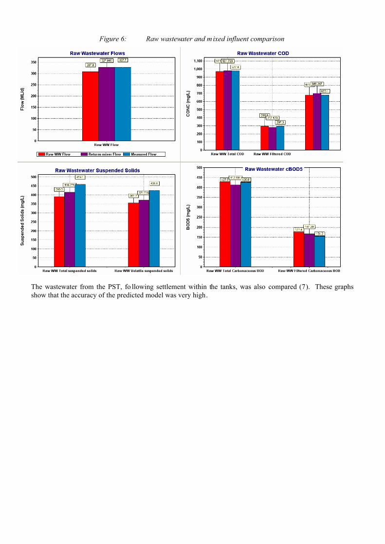
Figure 6: Raw wastewater and mixed influent comparison

The wastewater from the PST, fo llowing settlement within the tanks, was also compared (7). These graphs show that the accuracy of the predicted model was very high.

Figure 7: Liquid stream from PST prior to mixing in the IPS

3.1 FRACTION COMPARISONS Figure8 shows the comparison of mass fractions calculated from the measured values and predicted by BioWin. For the incoming wastewater the differences between p redicted and measured fr actions is very small. However, variations in the PST and IPS streams are more significant. Within the PST and IPS this can be traced back to the uncertainty with the predicted cBOD concentrations. Increased cBOD increases the amount of slowly biodegradable substrate available and decreases the inert COD fractions.

Figure 8: Predicted and measured mass fraction comparisons

4 APPLICATION

The calibrated BioWin model was sought after to enable its assistance with asset management and operations decision-making. Watercare was familiar with the application of modelling to other parts of the business, and the importance of calibration and also validation was recognised from this experience. Fund amentally:

• A model without calibration is a fantasy-world view, and is useful for demonstration of concept only

• A calibrated model without validation is an invalid real-world view and is useful for proof of concept

• A calibrated, validated model is a valid real-world view and is useful for future prediction

4.1 ASSET MANAGEMENT USE Watercare applied the calibrated model to prove the concept of capacity limit prediction within the Mangere WWTP. The results generated by this application allowed Watercare to reprioritise the assets under review for future expansion to meet expected growth in the wastewater catchments. It is now planned to period ically repeat the concept of capacity limit prediction using BioWin. The model may evolve and b e updated to reflect significant plant or process changes, and if so re-calibration will be required ahead of the next capacity review.

Figure 9: Predicted process limits from capacity modelling in BioWin and Excel

2005 2010 2015 2020 2025 2030 2035 2040 2045

Type

of L

imit

Year

DAF - Solids Loading Capacity Winter

BLENDED SLUDGE THICKENER - Solids Loading Capacit y

4 BLOWERS - Air Supply rate (Summer)

ZONE 2 DIFFUSERS - Air Flow Per Diffuser (Summer)

BLENDED SLUDGE THICKENER - Av erage Tot al Solids Lo ading Capac ity (Su mmer)

DIGESTERS - Hydra ulic Retentio n Time (Summer)

DAF Solids Loading Capacity (Summer)

INTERSTAGE PUMPING STATION - Peak Hydraulic Loading Capacity

TERTIARY FILTERS - Average Hydraulic Loading Capacity

Effluent Flow - Av erage Daily Flow

PRIMARY SEDIMENTATION TANKS - Solids Loa ding ra te

DIGESTERS - VSS L oading Rate ( Summer)

4 BLOWERS - Overall Air Supply rate (Winter)

PRIMARY SEDIMENTATION TANKS - Average Overf low Rate

5 BLOWERS - Overall Air Supply rate (Winter)

Total N Mass Load - maximum monthly mean (summer)

DIGESTERS - Hydraulic Retention Time (Winter)

Total N - maximum monthly mean (summer)

DIGESTERS - VSS Loading Rate ( Winter)

BLENDED SLUDGE THICKENER - Hydr aulic C apacit y (Win ter)

4.2 OPERATIONS USE Watercare also applies the calibrated model to test the whole-plant effect of proposed process changes and refinements. As discussed above, there are significant effects on downstream processes from altering the activated sludge process, and due to the plant recycles, there are significant upstream effects as well. It is very difficult to evaluate these effects without trialling and testing, which is expensive, slow and risky compared to evaluation using a calibrated model. The model may not predict accurately without being validated, but it does highlight what needs to be checked o ut from an operational view, and provides sufficient guidance to determine whether the modification is a good idea for Watercare to pursue.

4.2.1 STRUVITE DEPOSITION One concrete example of this is struvite deposition on equipment fro m the WAS. Prior to the BioWin model, the quantities of struvite that were deposited on the inside of certain pipes and tank walls were known to b e at nuisance levels. Measurement after the various cleans indicated that there was hundreds of tonnes per year, although the measurement was prone to error because the deposition was not uniformly struvite, and the deposition was scattered during clean-up. It was observed that a significant proportion of the struvite that was produced was not deposited at all, instead exiting the process as biosolids.

The BioWin model predicted that there was thousands o f tonnes of struvite produced per year, and has led to an evaluation (in progress) of whether there is an opportunity for process improvement to either eliminate or extract the struvite before it becomes a nuisance.

4.2.2 REACTOR TUNING In a related application, the activated sludge process is designed to remove nitrogen, and it is believed that unexpected “luxury uptake” of phosphorus pr ovides the substrate for struvite formation. The reactors are configured as step feed, with four anoxic and four aerobic zones interspersed with each other prior to clarification. The consent for discharge to the harbour carries a condition that the plant will limit total nitrogen, so any scarcity of COD for the nitrifying and denitrifying bacteria threatens this.

Watercare plans to use the BioWin model to investigate minor reconfigurations to the reactors to limit phosphorus uptake and maximise nitrogen removal to meet consent. The calibrated BioWin model, as mentioned above, predicts significant struvite formation from the WAS. It has been seen that “turning off” the phosphorus accumulating organisms (PAOs) reduces this, and therefore in its calibrated form, the model predicts phosphorus uptake in the reactor.

5 CONCLUSIONS

A calibrated full plant model of the Mangere wastewater treatment plant has been developed using the methods and protocols developed by WERF. In particular the intensive sampling and SBR protocols were used to build the calibration. The complexity of the treatment process and the interdependence of the unit processes meant that a large number of samples and analyses were needed around the plant to establish the calibrated wastewater fractions.

The model has been successfully used for fu ture capacity planning and has been used for the investigation of struvite formation at the plant. The mod el is also being used by process contro llers to evaluate “what if” scenarios and support process decisions.

REFERENCES EnviroSim 2008 - http://www.envirosim.com/products/bw32/bw32intro.php website live 22/05/08

EnviroSim 1991 - User Manual for BioWin 2.1, EnviroSim Associates Ltd.

Water Environment Research Foundation - Methods for Wastewater Characterization in Activated Sludge Modelling, 2003

McCoy M., Nutt D., Kumarasingham S., Mates M. 2007. The Advantages of having a Biological Wastewater Treatment Model from a Water Company Perspective. NZWWA Conference, Rotorua, New Zealand.