Embed Size (px)
Citation preview

7609 2019
April 2019
Urbanization, productivity differences and spatial frictions Calin Arcalean, Gerhard Glomm, Ioana Schiopu

Impressum:
CESifo Working Papers ISSN 2364-1428 (electronic version) Publisher and distributor: Munich Society for the Promotion of Economic Research - CESifo GmbH The international platform of Ludwigs-Maximilians University’s Center for Economic Studies and the ifo Institute Poschingerstr. 5, 81679 Munich, Germany Telephone +49 (0)89 2180-2740, Telefax +49 (0)89 2180-17845, email [email protected] Editor: Clemens Fuest www.cesifo-group.org/wp
An electronic version of the paper may be downloaded · from the SSRN website: www.SSRN.com · from the RePEc website: www.RePEc.org · from the CESifo website: www.CESifo-group.org/wp

CESifo Working Paper No. 7609 Category 2: Public Choice
Urbanization, productivity differences and spatial frictions
Abstract We study decentralized and optimal urbanization in a simple multi-sector model of a rural-urban economy focusing on productivity differences and internal trade frictions. We show that even in the absence of the typical externalities studied in the literature, such as agglomeration, congestion or public goods, the decentralized city size can be either too large or too small relative to that chosen by a planner. In particular, optimal urbanization exceeds decentralized levels when productivity differences in location specific non-traded goods is small, a case typically arising in developed economies. In contrast, developing countries are likely to display overurbanization. A numerical exercise calibrated to Brazilian data suggests that the wedges can be quantitatively important. Urban biased policies - placing a higher weight on the welfare of city dwellers - are closer to optimal policies than decentralized allocations whenever productivity differences in non-traded sectors are either very small or very large. For intermediate productivity differences, the urban bias leads to larger cities even relative to decentralized policies.
JEL-Codes: R120, R130, O180, J610.
Keywords: city size, productivity differences, multi-sector models, trade costs, welfare.
Calin Arcalean ESADE – Ramon Llull University
Spain - 08172 Sant Cugat [email protected]
Gerhard Glomm Indiana University
USA - 47405 Bloomington IN [email protected]
Ioana Schiopu
ESADE – Ramon Llull University Spain - 08172 Sant Cugat [email protected]
The authors acknowledge financial support from Universitat Ramon Llull, Banc Sabadell, the Spanish Ministry of Education and Science (ECO2016-76855-P) and Generalitat de Catalunya (2017 SGR 640). The usual caveat applies.
1 Introduction
Economic development the world over has been associated with ever-increasing rates
of urbanization. According to the U.N.’s The World Urbanization Prospects (2018), the
fraction of the population that lives in urban areas has increased from about 30% in
1950 to about 55% in 2018 and is expected to reach 68% by the year 2050. In Europe
and North America urbanization has already reached 74% and 82%, comparable with the
levels reached in Latin America and the Caribbean (81%) and Oceania (68%) while Asia
(50%) and Africa (43%) lag behind.
The size of cities and the associated degree of urbanization have been of interest to
academics at least since Beckmann (1972) and Mills and de Ferranti (1971). This issue
is also of great concern for policy makers. A recent report for the World Bank by Lall
and Shalizi (2006) poses the following questions regarding urbanization: “To what extent
is internal migration a desirable phenomenon and under what circumstances? Should
governments intervene and if so with what types of interventions? What should be their
policy objectives?”While there is a widespread consensus that urbanization represents
a great opportunity for economic progress, recent literature, such as Glaeser (2014) or
Fuller and Romer (2014) have emphasized the vital role of proper governance along the
way.
An abundant literature on optimal urbanization shed light on the effects of conges-
tion and scale economies1, public goods2, knowledge spillovers3, dynamic human capital
externalities or agglomeration forces4.
In this paper we take a step back and focus on how sector specific productivity dif-
ferences and trade frictions between urban and rural areas shape the allocation of people
1Seminal contributions by Mills and de Ferranti (1971) and Sheshinski (1973) consider models inwhich congestion influences optimal city size. In Henderson (1974), optimal city size balances scaleeconomies and increasing commuting costs for workers.
2Arnott (1979) embeds public goods considerations and transportation costs in an explicitly spatialmodel of city size. Poelhekke and Van der Ploeg (2008) focus on mega-cities and conclude that dueto insuffi cient public goods provision, urbanization is too large. Ott and Soretz (2010) obtain similarresults. Albouy et al. (2018) find in calibrated version of their model that US cities might well beunder-populated.
3Lucas (2001) models spatial structure, production externalities and choice of work sites and resi-dential locations. Following papers by Eaton and Eckstein (1997), Black and Henderson (1999), Glaeser(1999) and Lucas (2004), on “knowledge spillovers”in urban areas, Holmes (2005) estimates these effectsfor a particular activity, namely locating sales offi ces. Carlino and Hunt (2007) build on the idea ofknowledge spillovers and find a positive correlation between urban density and the rate of innovation.Berliant and Wang (2006) and Gautier and Teulings (2009) provide search theoretic micro-foundationsfor the knowledge spillovers mentioned above.
4In Drazen and Eckstein (1988), the competitive equilibrium allocation does not satisfy the GoldenRule and urbanization is too small relative to the Golden Rule. Following Lucas (1988) there is asizeable literature on city growth/urbanization that stresses the role of human capital externalities oragglomeration forces. This literature includes Glomm (1992), Lucas (2004), Fan and Stark (2008), Itoh(2009) and others. Depending on the precise specification of the agglomeration effects, urbanization mayexceed, fall short of, or be exactly equal to the optimal rate. Fan and Stark (2008), for example obtain“over-migration”since the migration of low skill workers can dilute the agglomeration effects.
2
across space, abstracting from any explicit externality or agglomeration effect.
Most of the literature on urbanization employs two location-two sector models under
the assumption that the urban area, hosting a so called modern sector (typically manu-
facturing), trades in a frictionless way with the rural area which is home to the traditional
sector (typically agriculture).
We generalize this framework in two ways. First, we allow for transportation costs
in the tradable sectors. Atkin and Donaldson (2015) provide evidence of large intra-
national frictions in developing countries. Focusing on Canada, Agnosteva and Yotov
(2019) demonstrate large differences in tradability across sectors. Second, we introduce
location specific, non-tradable sectors, possibly with different productivity levels.5
Local non-traded sectors are an important fraction of employment. Focusing on US
data, Jensen and Kletzer (2005) estimate that up to 60% of jobs are in non-traded
sectors, even after accounting for the tradability of some service sectors. In France,
Frocrain and Giraud (2017) estimate that the share of employment in non-traded sectors
can reach 50%−70% in metropolitan areas with larger shares in rural areas. For a sampleof Latin American countries, Reardon and Escobar (2001) document that the share of
rural non-farm income in total rural income is between 22% and 68%. Lanjouw and
Lanjouw (2001) disaggregate the non-farm rural sector and find that services, commerce
and transportation are often the lions’share of non-farm income. They also document
that in many countries the size of the non-farm rural sector is even expanding.
Differences in the level of productivity in the local non-traded sectors play a crucial
role. Consistent with the data, we assume that rural services are less productive than
urban services. There is a fundamental difference in productivity of small-scale local firms
between the city and the countryside. Much evidence points in the direction of lower
productivity in the countryside. Liedholm and Mead (1987) find that in three countries
net returns per hour worked are increasing as one moves from small rural localities with
fewer than 2, 000 inhabitants, to rural town with between 2, 000 and 20, 000 thousand
inhabitants, to cities with more than 20, 000 inhabitants. Productivities in the cities
sometimes exceed productivities in small rural localities by a factor of four. Porter and
Bryden (2004) find lower levels of wages in rural vs. urban areas and lower wage growth
rates as well. According to Wiggins and Proctor (2001) rural firms operate with lower
productivity than urban firms because of a lack of access to physical, human, financial
and social capital.
In our model both transportation costs and productivity differences determine the
allocation of people across space, which in turn has general equilibrium effects. An
individual’s move, for example, from the rural to the urban area, increases demand for
5This may arise due to agglommeration effects or sorting by skills. For example, Davis and Dingle(2017) show that cities have a comparative advantage over rural areas in skill intensive production. Inkeeping with the normative focus of the paper, we follow the literature (see for example Albouy et al.2018) and leave the microfoundations behind these productivity differences unspecified.
3
both traded and non-traded goods in the city. At the same time, it reduces the supply of
labor and thus the production of both traded and non-traded goods in the countryside.
As a result, the price of the rural traded good increases, which increases price indices in
both locations. How much these price indices go up in relative terms depends on both the
transportation costs for the traded goods and the productivity differences in non-traded
sectors across locations. In addition, the income in the rural area increases as it is directly
related to the price of the traded good.
We compare the decentralized equilibrium with the social planner’s solution. While
under decentralization migration stops when the level of utility is equalized across the two
regions, migrants do not take into consideration how this combination of price and income
effects changes with their decision. Therefore, the resulting competitive equilibrium is,
in general, not Pareto optimal. In other words, under decentralization, migration equal-
izes the average utility in the city and the countryside, while the social planner, which
is concerned with aggregate welfare, aims to balance marginal welfare across locations.
Whether the decentralized equilibrium produces over or under urbanization depends on
the productivity differences between sectors and the size of transportation costs. Specif-
ically, decentralized urbanization is too low when productivity differences in the two
non-traded sectors are small or when trading costs are relatively higher for the rural
good. As productivity differences between urban and rural areas tend to decline with
development, our results suggest that, for given transportation costs, the optimal city
size is smaller than the decentralized equilibrium at low development levels but larger in
developed economies.
Removing both transportation frictions in traded sectors and productivity differences
in non-traded sectors restores the optimality of decentralized urbanization. This is due
to the fact that prices of both traded and non-traded goods, as well as wages, fully reflect
the changes in demand and supply - for both goods and labor - arising from relocation
of agents. Thus, in this symmetric and frictionless case, geographical space no longer
matters and utility equalization across locations also implies income equalization.
Allowing only for transportation frictions introduces a wedge between the purchasing
power across locations, which depends on the allocation of people across locations and is
ignored under decentralization. Assuming rural goods are more costly to ship than urban
goods, the planner chooses a larger city relative to decentralization.
Nonetheless, when allowing for differences in both transportation costs and labor
productivity in non-traded sectors, the planner may prefer a smaller city.
In particular, assuming city-based non-traded sectors are more productive leads,
everything else equal, to a larger city which in turn leads to further reallocation of labor
across sectors within each region. Intuitively, "too many" people are employed in the
non-traded sector in the city while the opposite holds in the countryside. This leads to
lower employment in rural traded sectors and to the corresponding increase in the relative
4
price of these goods. Furthermore, the two mechanisms interact with one another, as the
effects of productivity differences in non traded sectors are magnified by the asymmetry
in transportation costs.
We complement the theoretical analysis with a simple quantitative exercise that al-
lows us to gauge the importance of productivity difference and trade frictions for optimal
urbanization. We rely on data from the Brazilian 1980 census to compute sectoral em-
ployment allocations across urban and rural areas. We parametrize the model to match
these data in conjunction with other macroeconomic indicators under decentralized poli-
cies. The benchmark parameter values are consistent with significant differences in both
productivity and trade frictions. Counterfactual numerical exercises suggest an optimal
share of urban population 22% larger than that observed in the data. On the other
hand, removing completely trade frictions while maintaining productivity differences in
non-traded sectors results in the optimal urbanization being almost 5% smaller than the
corresponding decentralized urbanization rate.
Finally, we relate our model to the literature on "urban-biased" policies by construct-
ing a social planner’s problem where the welfare of the city dwellers has a higher weight.
We compare this "urban-biased" policy against decentralized and optimal policies. Inter-
estingly, we find that relative to decentralization, urban biased policies yield allocations
that move in the direction of optimal policies in advanced or very poor economies, i.e.
when productivity differences in non-traded sectors are either very small or very large. In
contrast, at intermediate levels of development, the urban bias results in too large cities
relative to the optimal solution, which in turn is lower than the decentralized city size.
In the following section, we introduce the model. In section 3, we define and solve for
the decentralized equilibrium and show it is unique. In section 4, we define the centralized
optimum. In section 5, we compare the decentralized and the centralized regime. Section
6 illustrates the theoretical findings with a numerical example calibrated on Brazilian
data. In section 7, we discuss "urban-biased" policies. Section 8 contains concluding
remarks with directions for future work. Proofs and derivations are contained in the
appendix.
2 A model of labor allocation across space and sec-
tors
There are two locations, urban (u) and rural (r). Each is inhabited by mobile house-
holds with total mass normalized to unity. Each location produces one traded and one
non-traded good. For simplicity, we label the urban traded good b, the rural traded good
a and the region specific non-traded goods nu and nr respectively. These goods repre-
sent a broad mix of sectors, reflecting for example, the fact that the urban areas may
5

produce a range of manufactured goods and services while the rural area will export, in
addition to agriculture, some services and even manufactured goods. See, for example,
Kolko (1999) and Henderson (2010). In our numerical examples we use an empirical
tradability index developed in Gervais and Jensen (2015) to group various sectors into
tradable/non-tradable.Households in each region derive utility from consumption of the two traded goods
and from the region specific non-traded good. There are iceberg trade costs associated
with shipping the tradable goods between regions, τ b and τa, where τ b > 1 and τa > 1,
i.e. if urban dwellers want to consume one unit of the rural traded good, they need to
buy τa units. We assume that in each region labor markets are competitive and labor
moves freely between sectors until wages are equalized.
Individuals. The urban residents maximize:
Uu(bu, au, nu) =[(bu)θ + (au)θ + (nu)θ
]1/θ, (1)
where bu, au and nu are consumption of traded urban good b, rural traded good a, and
the urban non-traded good nu, respectively. In the following, we assume that goods are
substitutes in consumption, i.e. θ ∈ (0, 1].6 The elasticity of substitution is e = 1/(1− θ).We assume the urban traded good is the numeraire and normalize pb = 1. The budget
constraint of the urban consumer is:
bu + paτaau + pnun
u = Iu, (2a)
where pa and pnu are the relative prices of a and nu respectively. The term τaau is the
quantity of good a that city dwellers buy in order to consume au units. Iu is the income
of an urban resident.
Preferences of individuals in the rural area are identical to those in the urban area
and given by:
U r(br, ar, nr) =[(br)θ + (ar)θ + (nr)θ
]1/θ, (3)
where br, ar and nr are consumption of the urban good, rural traded and the rural
non-traded good, respectively. The corresponding budget constraint is:
τ bbr + paa
r + pnrnr = Ir, (4)
while pa and pnr are the corresponding relative prices. The term τ bbr is the quantity of
traded urban good that consumers in the rural area buy in order to consume br units. Ir
is the income of a resident in the rural area.
Production. There are four production technologies in this economy, all of them6This is in line with the recent trade literature, e.g. Costinot and Rodriguez-Clare (2014).
6
are linear in labor: Yb = AbLb, Ya = AaLa, Ynu = AnuLnu and Ynr = AnrLnr, where Lb,
La, Lnu and Lnr are employment allocations in the b-sector, a-sector and the urban and
rural non-traded sectors, respectively. Ab, Aa, Anu and Anr are the corresponding sectoral
exogenous productivities. In each sector there are competitive firms that maximize profits
taking prices as given.
Assumption 1. Productivity in the urban non-traded sector is higher than that in therural non-traded sector: Anu > Anr.
This assumption is consistent with empirical evidence by Liedholm and Mead (1987),
Ciccone and Hall (1996), Wiggins and Proctor (2001), and Porter and Bryden (2004).
In the following, we analyze and compare three regimes: 1) the decentralized equilib-
rium, where households freely choose their region of residence, 2) the centralized optimum,
where a social planner chooses the allocation of people between city and rural area that
maximizes the aggregate welfare in the economy and 3) an "urban biased" regime where
the social planner attaches a higher weight on the welfare of the city inhabitants.
3 Decentralized equilibrium
Denote with φ the mass of people residing in the urban region (the size of the city).
As the total population in the economy is normalized to 1, φ ∈ (0, 1).Labor market clearing implies: φ = Lb+Lnu , and 1−φ = La+Lnr. Denoting by φnu
the fraction of people in the city working in the non-tradable sector, we can write
Lnu = φnuφ (5)
and
Lb = (1− φnu)φ. (6)
Similarly,
Lnr = φnr(1− φ) (7)
and
La = (1− φnr)(1− φ). (8)
Next, we solve the consumers’problems in the two regions. Denote γ = θ/(θ− 1) < 0when θ ∈ (0, 1]. The demands for tradable and non-tradable goods in the city are:
bu = Iu1
1 + (τapa)γ + (pnu)γ, (9)
au = Iu(τapa)
γ−1
1 + (τapa)γ + (pnu)γ, (10)
7
nu = Iu(pnu)
γ−1
1 + (τapa)γ + (pnu)γ. (11)
In the rural area, the corresponding demand functions are:
br = Ir(τ b)
γ−1
(τ b)γ + (pa)γ + (pnr)γ(12)
ar = Ir(pa)
γ−1
(τ b)γ + (pa)γ + (pnr)γ(13)
nr = Ir(pnr)
γ−1
(τ b)γ + (pa)γ + (pnr)γ. (14)
In each sector, labor is paid the corresponding value of marginal product: wb = Ab,
wa = paAa, wnr = pnrAnr, wnu = pnuAnu, where wb, wa, wnr, and wnu are the wages in
the b-sector, a-sector, rural and urban non-traded sectors, respectively.
Now we define the decentralized equilibrium in which household freely decide their
location by comparing the corresponding utilities in each location. As household are
identical, in equilibrium the utility of residing in the city is equal to that in the rural
area.
Definition 1. A decentralized equilibrium consists of urban and rural households’con-
sumption allocations (bu, au, nu, br, ar, nr), prices of goods (pa, pnr, pnu), wages (wb, wa,
wnu and wnr), the fraction of labor residing in the city φ, sectoral employment shares
within regions (φsr, φsu), such that, given the exogenous trade costs τa and τ b, and the
exogenous sectoral productivities Ab, Aa, Anu and Anr :
1. households maximize utility subject to the budget constraint, given wages and the
prices of goods;
2. the competitive firms solve their optimization problem given the prices of goods and
wages;
3. wages are equalized across sectors;
4. all good markets clear;
5. the labor markets clear in each region;
6. households’utilities are equal across regions.
Next, we solve for the decentralized allocations. Wage equalization across sectors in
each region implies: wb = wnu and wa = wnr. Thus, the income of an urban resident is:
Iu = Ab = pnuAnu (15)
and the typical income in the rural area is:
Ir = paAa = pnrAnr. (16)
8
Thus, we can express pnu and pnr as functions of pa and sectoral productivities:
pnu =AbAnu
(17)
and
pnr = paAaAnr
. (18)
Market clearing in non-traded good in the urban area implies φsu = AnuLnu, where the
left-hand side is the quantity demanded and the right-hand side is the quantity supplied.
Substituting Lnu from (5) and demand for non-traded good in the urban area nu from
(11),we obtain:
φnu =Iu
Anu
(pnu)γ−1
1 + (τapa)γ + (pnu)γ.
Plugging in Iu = pnuAnu, we can write the employment share in non-traded sector in
the urban area as a function of prices and transportation frictions:
φnu =(pnu)
γ
1 + (τapa)γ + (pnu)γ.
By the same token, we obtain (1 − φ)nr = AnrLnr. Substituting Lnr from (7), the
demand for non-traded good in the rural area nr from (14) and Ir = pnrAnr, we obtain:
φnr =(pnr)
γ
(τ b)γ + (pa)γ + (pnr)γ.
We substitute (17) and (18) in the expressions of φnu and φnr and get:
φnu =( AbAnu)γ
1 + (τapa)γ + (AbAnu)γ
(19)
φnr =(pa
AaAnr)γ
(τ b)γ + (pa)γ + (paAaAnr)γ. (20)
Next, we use the market clearing of the urban traded good b to obtain a relationship
between the relative price pa and the share of urban population φ :
φbu + (1− φ)τ bbr = AbLb. (21)
The demand for good b in the urban and rural areas are, respectively:
bu =Ab
1 + (τapa)γ +(
AbAnu
)γ and br = paAa(τ b)γ−1
(τ b)γ + (pa)γ +(pa
AaAnr
)γ ,where we substituted the expressions for Iu, Ir, pnu and pnr (equations (15), (16), (17)
9
and (18), respectively). Next, we use the equation (19) for φnu to express Lb as a function
of the endogenous variables pa and φ :
Lb = (1− φnu)φ =1 + (τapa)
γ
1 + (τapa)γ +(
AbAnu
)γ φ.Plugging bu, br and Lb into the market clearing condition for good b, (21) and rear-
ranging terms yields:
(1− φ)φ
Aa(τ b)γ
Ab(τa)γ(pa)γ−1=(τ b)
γ + (pa)γ +
(pa
AaAnr
)γ1 + (τapa)γ +
(AbAnu
)γ . (22)
We express φ as a function of pa :
φ =Aapa(τ b)
γ[1 + (τapa)
γ +(
AbAnu
)γ]Aapa(τ b)γ
[1 + (τapa)γ +
(AbAnu
)γ]+ Ab(τa)γ(pa)γ
[(τ b)γ + (pa)γ +
(pa
AaAnr
)γ] .(23)
Finally, in the decentralized regime the utility is equalized across regions: Uu(bu, au, nu) =
U r(br, ar, nr).
We use the demand expressions for each good in the urban and rural areas (9), (10), (11), (12), (13)
and (14) to obtain the indirect utilities in the two regions:
V u = Iu
[1 + (τapa)
γ +
(AbAnu
)γ]− 1γ
(24)
and
V r = Ir
[(τ b)
γ + (pa)γ +
(paAaAnr
)γ]− 1γ
. (25)
Equalizing V u and V r and substituting (15) and (16) yields:
AbAapa
=
(τ b)γ + (pa)γ +(pa
AaAnr
)γ1 + (τapa)γ +
(AbAnu
)γ−
1γ
. (26)
The expression (26) pins down the equilibrium pa as a function of exogenous variables,
sectoral productivities and transportation costs. The proposition below establishes the
existence and uniqueness of the solution, as well as properties of pa.
Proposition 1. There exists a unique relative price pa > 0 that solves equation (26).
The equilibrium relative price pa is increasing in Anu and decreasing in Anr. Also, pa is
increasing in τ b and decreasing in τa.
Proof in the Appendix.
10
A unique pa implies a unique decentralized allocation of people across regions, φd.
The fact that φd ∈ (0, 1) can immediately be seen from studying equation (23).
Proposition 2. Denote by φd the share of urban population in the decentralized equilib-rium. There exists a unique interior φd ∈ (0, 1) that satisfies equation (23), where pa isgiven by (26). The decentralized share of urban population φd is increasing in pa.
Proof in the Appendix.
An increase in pa raises the demand for the urban traded good both in the city
and the country side, as well as the relative employment in this sector. When goods
are substitutes, trade balance implies a larger share of population residing in the city.7
In equilibrium, the relative price pa and the city size are determined jointly by utility
equalization and market clearing in tradables. Once the solutions for φd and pa are
found, the sectoral allocations of labor can be determined. The share of labor in urban
and rural non-traded goods are given by equations (19) and (20), respectively. Studying
the expressions (19) and (20), we can see that the share of labor in urban non-tradables
φnu is increasing in pa, while the opposite holds for φnr.
4 Centralized optimum
Now we focus on a centralized optimum, in which the fraction of people residing in the
city is chosen by a planner that maximizes the aggregate welfare in the economy subject
to wage equalization across sectors and clearing of labor and good markets.
Definition 2. A centralized optimum consists of urban and rural households’consumptionallocations (bu, au, nu, br, ar, nr), prices of goods (pb, pa, pnr, pnu), wages (wb, wa, wnu and
wnr), the fraction of people residing in the city φ, sectoral employment shares within
regions (φnr, φnu), such that, given the exogenous trade costs τa and τ b, and the exogenous
sectoral productivities Ab, Aa, Anu and Anr :
1. households maximize utility subject to the budget constraint given the prices of
goods,
2. the competitive firms solve their optimization problem given the prices of goods and
wages,
3. wages are equalized across sectors,
4. all good markets clear,
5. the labor markets clear in each region, and
6. the aggregate welfare function
W (φ) = φUu(φ) + (1− φ)U r(φ),
7The property also holds for moderate degrees of complementarity θ < 0, given transportation costsare not too large.
11
is maximized, where Uu and U r are the individual utilities in the urban and rural
areas.
Next, we substitute the urban and rural incomes Iu = Ab and Ir = paAa into equations
(24) and (25) to express the indirect utilities as functions of the relative price pa(φ) and
the exogenous parameters:
V u(φ) = Ab
[1 + (τapa(φ))
γ +
(AbAnu
)γ]− 1γ
(27)
V r(φ) = Aapa(φ)
[(τ b)
γ + (pa(φ))γ +
(pa(φ)
AaAnr
)γ]− 1γ
. (28)
Consequently, the social planner’s problem is:
maxφ
W (φ) = φV u(pa(φ)) + (1− φ)V r(pa(φ)), (29)
where V u(pa(φ)) and V r(pa(φ)) are given by (27) and (28), respectively, and pa(φ) satisfies
the market clearing condition in the urban traded sector, (22).
Proposition 3. Denote by φc the optimal share of urban population. There exists aninterior solution φc ∈ (0, 1) to the central planner’s problem (29).
Proof in the Appendix.
Proving uniqueness of the solution is challenging, as the functionW (φ) is not concave
over the entire interval (0, 1). However, simulations over the relevant parameter ranges
reveal that the solution of the central planner has a unique global maximum.
5 Comparison of regimes
In the following we compare the decentralized fraction of urban population with the
centralized optimum. We proceed by evaluating the slope of the aggregate welfare func-
tion ∂W (φ)/∂φ at the decentralized solution φd. If ∂W/∂φ|φ=φd > 0, then then social
planner prefers a bigger city than the one arising in the decentralized equilibrium, i.e.
φc > φd. The opposite holds when ∂W/∂φ|φ=φd < 0.Differentiating W with respect to φ yields:
∂W
∂φ= (1− φ)∂V
r(φ)
∂φ+ φ
∂V u(φ)
∂φ+ V u(φ)− V r(φ),
where V u(φ) and V r(φ) are given by (24) and (25).
When evaluating ∂W (φ)/∂φ at the decentralized allocation φd the last two terms
cancel as the decentralized allocation satisfies V u(φd) = V r(φd). Thus, ∂W/∂φ|φ=φd
12
becomes:
∂W
∂φ
∣∣∣∣φ=φd
= (1− φd)∂V r(φ)
∂φ
∣∣∣∣φ=φd
+ φd∂V u(φ)
∂φ
∣∣∣∣φ=φd
(30)
= −V r(φd)(1− φd)(pa)γ−1
(τ b)γ + (pa)γ +(pa
AaAnr
)γ [1 + ( AaAnr
)γ]∂pa(φ)
∂φ
∣∣∣∣φ=φd
+ V r(φd)(1− φd)
pa
∂pa(φ)
∂φ
∣∣∣∣φ=φd
− V u(φd)φd(pa)
γ−1(τa)γ
1 + (τapa)γ +(
AbAnu
)γ ∂pa(φ)
∂φ
∣∣∣∣φ=φd
,
where we used the fact that (1− θ) γ/θ = −1.The expression above shows that the under decentralization the marginal worker
ignores the effects of her migration decision on the other agents, both in the rural and
the urban region. The terms in the expression above illustrate these effects that work
through the prices. Intuitively, there are direct effects on prices that consumers pay and
indirect effects on workers’incomes.
Consider a marginal increase in the size of the city φ. As shown in Proposition 2,
a higher city size φ has a positive effect on the relative price of rural traded good pa(∂pa(φ)/∂φ|φ=φd > 0
). Wage equalization in the rural area implies a higher price of
rural non-traded goods pnr. Higher prices have a negative effect on consumers’welfare
V r, which is reflected in the first term in the expression above. At the same time, as pagoes up, the incomes in the rural area increase
(∂Ir/∂φ = Aa ∂pa(φ)/∂φ|φ=φd > 0
).
In the urban area, a higher φ has a negative effect on welfare, driven by a higher
relative price of the traded good pa. There is no income effect or an effect through the
price of tradables as the urban traded good is the numeraire. As the production functions
are linear in labor, the relative price of urban non-traded sectors pnu is constant.8
Using the fact that V u(φd) = V r(φd) and1−θθγ = −1, we can rewrite ∂W
∂φ
∣∣∣φ=φd
as:
∂W
∂φ
∣∣∣∣φ=φd
= V u(φd)
−φd(τa)
γ(pa)γ−1
1 + (τapa)γ +(
AbAnu
)γ︸ ︷︷ ︸individual price effect on Vu
− (1− φd)×
×
[1 +
(AaAnr
)γ](pa)
γ−1
(τ b)γ + (pa)γ +(pa
AaAnr
)γ︸ ︷︷ ︸
individual price effect on Vr
+ (1− φd)1
pa︸︷︷︸individual income effect on Vr
∂pa(φ)
∂φ
∣∣∣∣φ=φd
.
(31)
8A production function with decreasing returns in factors would generate an income effect, as well achange in the price of services.
13
Combining the price and the income effect in the rural area yields the net effect on
individual welfare: (τb)γ
pa
((τ b)
γ + (pa)γ +
(pa
AaAnr
)γ)−1> 0.
Consequently, the net effect of a marginal increase of φ on the utility in the rural area
is positive, that is, the positive income effect outweighs the negative price effect.
Thus, the net aggregate welfare effect of a marginal change in the size of the city at
φ = φd depends on the magnitude of opposite effects on individual welfare in each region,
as well as their weights (φd and 1− φd), which depend on the magnitudes of the spatialfrictions present in the model (the trade costs and the productivity gap between the rural
and urban areas). When the net change is positive, ∂W∂φ
∣∣∣φ=φd
> 0, the centralized solution
φc is higher than the decentralized one, φd. The opposite holds when∂W∂φ
∣∣∣φ=φd
< 0.
Next, we rewrite
∂W
∂φ
∣∣∣∣φ=φd
=V u(φd)(pa)
γ−1
1 + (τapa)γ +(
AbAnu
)γ︸ ︷︷ ︸
D>0
−φd(τa)γ
+(1− φd)(τb)
γ
(pa)γ
1+(τapa)γ+(AbAnu
)γ(τb)γ+(pa)γ+(pa Aa
Anr)γ
∂pa(φ)
∂φ
∣∣∣∣φ=φd
and use the fact that φd satisfies the market clearing condition for the urban traded
good:
(1− φd)φd
Aa(τ b)γ
Ab(τa)γ(pa(φd))γ−1 =
(τ b)γ + (pa(φd))
γ +(pa(φd)
AaAnr
)γ1 + (τapa(φd))
γ +(
AbAnu
)γ .
We obtain:
∂W
∂φ
∣∣∣∣φ=φd
= D
{−φd(τa)γ
+(1− φd)(τb)
γ
(pa)γφd
(1−φd)Ab(τa)
γ(pa)γ−1
Aa(τb)γ
}∂pa(φ)
∂φ
∣∣∣∣φ=φd
= Dφd(τa)γ(pa)
−1(AbAa− pa
)∂pa(φ)
∂φ
∣∣∣∣φ=φd
In the proof of Proposition 2 we have shown that ∂φ/∂pa > 0. Thus,∂pa(φ)∂φ
∣∣∣φ=φd
> 0.
Therefore, sign[∂W∂φ
∣∣∣φ=φd
]= sign
(AbAa− pa(φd)
).
The following proposition states the conditions under which the planner prefers a
larger (smaller) city than the decentralized solution.
Proposition 4. The social planner prefers a larger city than the decentralized outcome(φc > φd) when the following condition holds:
(Anu)−γ − (Anr)−γ < (Aa)−γ [1− (τa)γ]− (Ab)−γ [1− (τ b)γ] , (32)
where θ ∈ (0, 1) and γ = θ/(θ − 1) < 0.
14
Proof in the Appendix.
When Anr < Anu, Aa < Ab and τa > τ b, inequality (32) is more likely to hold when the
productivity difference in non-tradables is small. Also, the condition is more likely to hold
when the iceberg costs in non-tradables τa are large relative to τ b, and the productivity
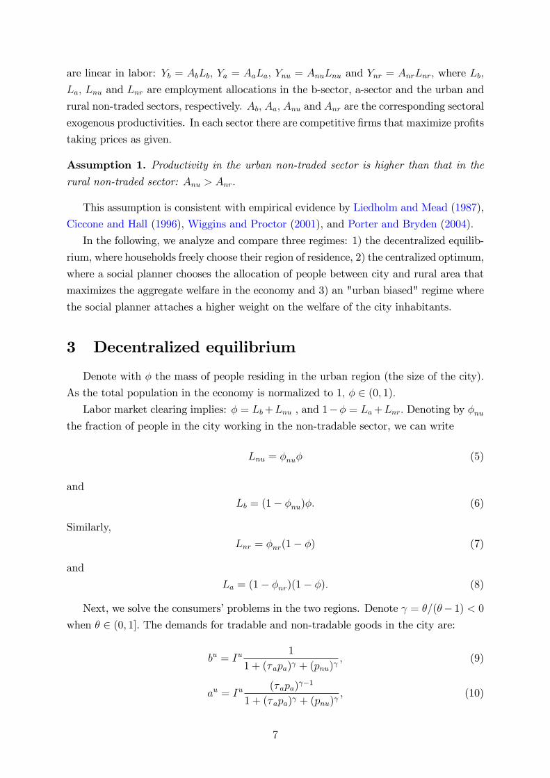
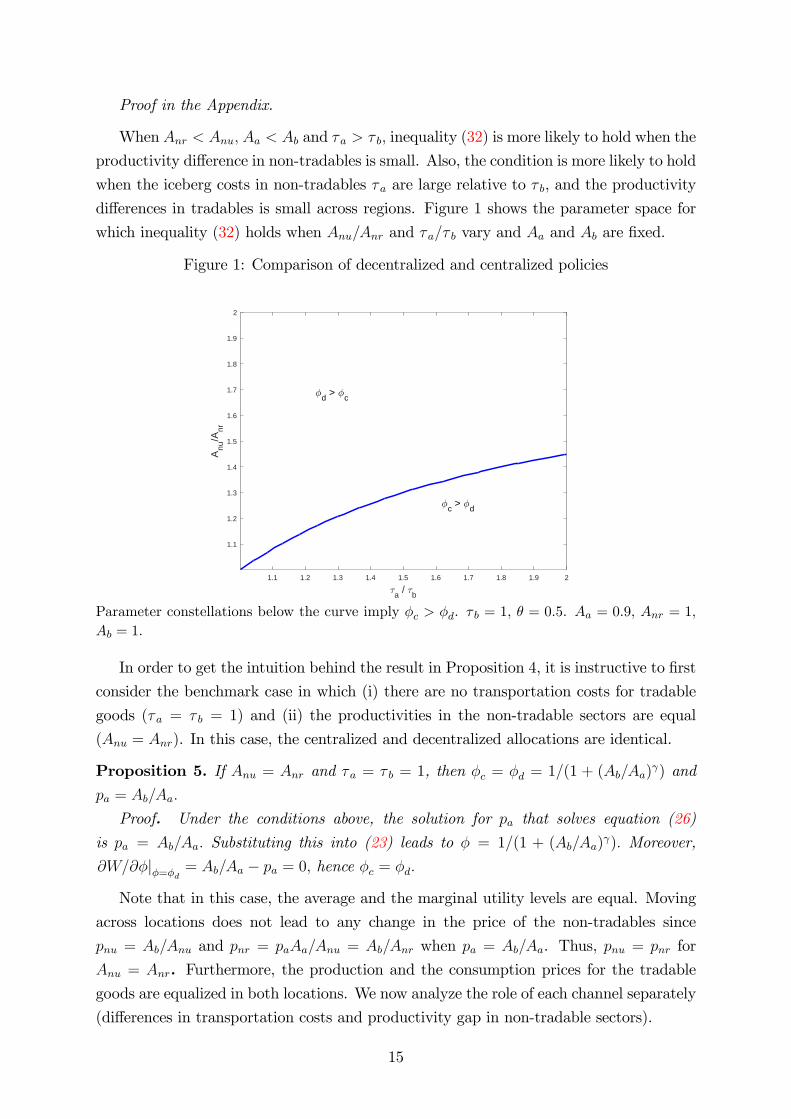
differences in tradables is small across regions. Figure 1 shows the parameter space for
which inequality (32) holds when Anu/Anr and τa/τ b vary and Aa and Ab are fixed.
Figure 1: Comparison of decentralized and centralized policies
1.1 1.2 1.3 1.4 1.5 1.6 1.7 1.8 1.9 2
a /
b
1.1
1.2
1.3
1.4
1.5
1.6
1.7
1.8
1.9
2
Anu
/Anr
c >
d
d >
c
Parameter constellations below the curve imply φc > φd. τ b = 1, θ = 0.5. Aa = 0.9, Anr = 1,Ab = 1.
In order to get the intuition behind the result in Proposition 4, it is instructive to first
consider the benchmark case in which (i) there are no transportation costs for tradable
goods (τa = τ b = 1) and (ii) the productivities in the non-tradable sectors are equal
(Anu = Anr). In this case, the centralized and decentralized allocations are identical.
Proposition 5. If Anu = Anr and τa = τ b = 1, then φc = φd = 1/(1 + (Ab/Aa)γ) and
pa = Ab/Aa.
Proof. Under the conditions above, the solution for pa that solves equation (26)
is pa = Ab/Aa. Substituting this into (23) leads to φ = 1/(1 + (Ab/Aa)γ). Moreover,
∂W/∂φ|φ=φd = Ab/Aa − pa = 0, hence φc = φd.
Note that in this case, the average and the marginal utility levels are equal. Moving
across locations does not lead to any change in the price of the non-tradables since
pnu = Ab/Anu and pnr = paAa/Anu = Ab/Anr when pa = Ab/Aa. Thus, pnu = pnr for
Anu = Anr. Furthermore, the production and the consumption prices for the tradablegoods are equalized in both locations. We now analyze the role of each channel separately
(differences in transportation costs and productivity gap in non-tradable sectors).
15
First, when τa = τ b = 1 but Anu 6= Anr, and in particular Anu > Anr, the right-hand
side of inequality (32) becomes zero while the left-hand side is positive, thus the planner
prefers a smaller city (φ) and a lower price for the rural tradable good (pa) than in the
decentralized regime. As we have shown in Proposition 1, the price pa is increasing in Anu.
Consider a change from a benchmark in which Anu = Anr to a situation in which Anu is
higher and Anr stays the same (such that now Anu > Anr). The resulting decentralized paincreases relative to the benchmark, which yields a higher decentralized φd. The marginal
migrant - which takes prices and incomes as given - ignores the general equilibrium effect
of the increase in pa on the welfare of both city and countryside residents. We can see
from expression (31) that a higher Anu magnifies the negative price effect in the individual
welfare in the city. Also, a higher decentralized φd implies a larger aggregate price effect
in the city, and a smaller positive net effect on rural welfare (lower 1−φd). Consequently,the negative welfare effect in the city offsets the positive effect in the rural area and the
planner chooses a lower pa and a smaller city size than the decentralized equilibrium. The
larger the productivity difference in non-tradables between the rural and urban areas, the
lower the city size preferred by the planner.
Second, consider the case of Anu = Anr and τa > τ b = 1 (there are positive trans-
portation costs only for the tradable good produced in the rural area). The left-hand
side of inequality (32) becomes zero while the right-hand side is positive, thus the plan-
ner prefers a larger city (φ) and a higher price for the rural tradable good (pa) than in
the decentralized regime. As equilibrium pa is decreasing in τa (see Proposition 1), the
resulting decentralized φd and pa are lower than in the frictionless benchmark. At φd, a
marginal increase in φ has a positive welfare effect in the rural area and negative in the
city (see equation 31) that are ignored by the marginal migrant. However, the aggre-
gate positive effect in the rural area dominates, as 1 − φd is larger, and the planner canincrease aggregate welfare by choosing a larger city. A larger productivity Aa magnifies
the positive welfare effect in the rural area from having a larger city and makes social
planner’s solution (φc) even larger relative to the decentralized one (φd).
Positive transportation costs in the tradable good produced in the city (τ b > 1) change
the effects discussed above in the opposite direction. The net effect (and the optimal city
size) depends on the productivity difference in the tradable sectors (Aa relative to Ab)
and the difference in trade costs. For example, if the differences in transportation costs
are large and productivity differences in tradables are small (Aa is large relative to Aband τa is large relative to τ b), then the planner prefers a bigger city.
As the magnitude of productivity differences varies with the level of development,
these results have implications on the optimal urban policies along the development path.
While direct evidence on rural-urban productivity differences at sector level is scant,
more developed economies have in general a more uniform distribution of industries across
space (see Imbs et al. (2012)). Furthermore, the productivity differences across sectors
16
do vary with the level of development. For example, Acemoglu and Zilibotti (2001)
document that the productivity differences between manufacturing (more concentrated
in the city) and agriculture (more concentrated in the rural areas) are more pronounced
in developing economies than in the more advanced ones. Finally, Duarte and Restuccia
(2019) find that cross-country productivity differences are much larger in non-traded vs.
traded services.
Therefore, we would expect Anu/Anr to be inversely related to the level of develop-
ment. In this case, as shown in Figure 1, our results imply that, at a given level of
transportation costs, the optimal city size is smaller than the decentralized equilibrium
at low development levels (Anu/Anr large) and larger in developed economies (Anu/Anrsmall). The implication for advanced levels of development echoes, at an aggregate level,
the result in Albouy et al. (2018), who find that most of the cities in the US are too small.
However, while their model relies on a mix of location and fiscal externalities, our results
stem from the interplay of transportation frictions and productivity differences between
regions.
At intermediate levels of development, the ranking of decentralized and optimal ur-
banization depends on the relative transportation costs of the two tradable goods. Thus,
for example, in a large economy, rural tradable goods, such as agricultural products or
other natural resources, are likely to face larger transportation even at higher levels of
development and thus φc > φd. The numerical example presented in the next section,
calibrated using data from Brazil, approximates well such a case.
6 A numerical example
In this section we provide a numerical illustration of the model using data from Brazil
in the 80s. Although the model is stylized, this exercise allows us to gauge the quantitative
importance of the frictions at work.
We start by calibrating the decentralized version of the model to broadly match sec-
toral data on employment and productivity across urban and rural areas. Next, we use
the calibrated parameters values to back out the optimal city size implied by our model.
The model’s parameters are the sectoral labor productivity levels Ab, Anu, Aa and
Anr, the transportation costs τa and τ b and θ, driving the elasticity of substitution. In
the following we normalize Ab = 1 and use θ = 0.8 implying an elasticity of substitution
of 5.9 The rest of the model’s parameters are calibrated as follows.
We use Brazilian census data from 1980, available from IPUMS-International to com-
pute the distribution of workers across sectors and space.10
9We follow parametrizations used in the recent quantitative trade literature, e.g. Albrecht andTrevor Tombe (2016) and Costinot and Rodriguez-Clare (2014).10See IPUMS (2018) for details on the IPUMS-International database.
17
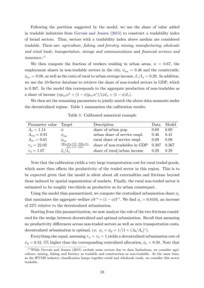
Following the partition suggested by the model, we use the share of value added
in tradable industries from Gervais and Jensen (2015) to construct a tradability index
of broad sectors. Thus, sectors with a tradability index above median are considered
tradable. These are: agriculture, fishing, and forestry, mining, manufacturing, wholesale
and retail trade, transportation, storage and communications and financial services and
insurance.11
We then compute the fraction of workers residing in urban areas, φ = 0.67, the
employment shares in non-tradable sectors in the city, φnu = 0.46 and the countryside,
φnr = 0.09, as well as the ratio of rural to urban average income, Ir/Iu = 0.29. In addition,
we use the 10-Sector database to retrieve the share of non-traded sectors in GDP, which
is 0.307. In the model this corresponds to the aggregate production of non-tradables as
a share of income (φpnunu + (1− φ)pnrnr)/(φIu + (1− φ)Ir).We then set the remaining parameters to jointly match the above data moments under
the decentralized regime. Table 1 summarizes the calibration results:
Table 1: Calibrated numerical example
Parameter value Target Description Data ModelAa = 1.14 φ share of urban pop. 0.69 0.69Anu = 0.91 φnu urban share of service empl. 0.46 0.41Anr = 0.61 φnr rural share of service empl. 0.09 0.08
τa = 22.03φpnunu+(1−φ)pnrnr
φIu+(1−φ)Ir share of non-tradables in GDP 0.307 0.367
τ b = 1.07 Ir/Iu share of rural/urban income 0.29 0.29
Note that the calibration yields a very large transportation cost for rural traded goods,
which more then offsets the productivity of the traded sector in this region. This is to
be expected given that the model is silent about all externalities and frictions beyond
those induced by spatial segmentation of markets. Finally, the rural non-traded sector is
estimated to be roughly two-thirds as productive as its urban counterpart.
Using the model thus parametrized, we compute the centralized urbanization share φcthat maximizes the aggregate welfare φV u+ (1− φ)V r.We find φc = 0.8416, an increase
of 22% relative to the decentralized urbanization.
Starting from this parametrization, we now analyze the role of the two frictions consid-
ered for the wedge between decentralized and optimal urbanization. Recall that assuming
no productivity differences across non-traded sectors as well as zero transportation costs,
decentralized urbanization is optimal, i.e. φc = φd = 1/(1 + (Ab/Aa)γ).
Everything else equal, assuming τa = τ b = 1 yields a decentralized urbanization rate of
φd = 0.52, 5% higher than the corresponding centralized allocation, φc = 0.50. Note that
11While Gervais and Jensen (2015) exclude some sectors due to data limitations, we consider agri-culture, mining, fishing and forestry as tradable and construction as non-tradable. At the same time,as the IPUMS industry classification lumps together retail and wholesale trade, we consider this sectortradable.
18

in this case, urbanization is lower under both regimes as the demand for rural tradable
good increase and so does the income in the rural area. Intuitively, a reduction in the
transportation costs for goods produced in rural areas, be it exogenous or policy driven,
could imply the need to adjust the urbanization policies as the decentralized population
distribution may be suboptimally skewed towards cities.
While in-depth policy analysis is beyond the scope of this framework, the numeri-
cal exercise suggests nonetheless that spatial productivity differences and transportation
costs could potentially generate significant departures from optimal urbanization rates.
7 The urban bias
The city dwellers and the inhabitants of the rural area have conflicting interests re-
garding the size of the city, as the individual welfare in the urban area V u(φ) is decreasing
in φ, while the opposite is true for V r(φ). Starting with the seminal contribution of Lipton
(1977), this tension has long been noted in the development literature, for example in
Yang (1999)) or Bezemer and Headey (2008). In the spirit of this literature, we analyze
the case when the central planner has an "urban bias", that is, it puts a higher weight
on the total welfare in the city. Consequently, the social planner’s problem with urban
bias becomes:
maxφp
W p(φ) = δφV u(pa(φ)) + (1− δ)(1− φ)V r(pa(φ)), (33)
where V u(pa(φ)) and V r(pa(φ)) are given by (27) and (28), respectively, and pa(φ) satisfies
the market clearing condition in the urban traded sector, (22). Also, in the case of urban
bias δ > 1/2.
Denote by φp the solution chosen by the urban biased planner. It can be shown that
an interior solution always exists in the interval (0, 1). The proof is similar to that of
Proposition 3.
Proposition 6. φp > φd when (Anu)−γ−(Anr)−γ < (Aa)−γ [1− κ−γ(τa)γ]+(Ab)−γ [κ−γ(τ b)γ − 1] ,
where κ = (1−δ)/δ < 1 and δ > 1/2. The condition is suffi cient but not necessary. Whenthe condition holds, also φc > φd.
Proof in the Appendix.
The condition is more likely to hold when the difference in productivities between the
non-tradable sectors is small, or when τa is large relative to τ b. In this case, the urban
bias leads to a city size that is larger than the decentralized equilibrium (φp > φd), while
the central planner also prefers a large city size (φc > φd).
Ranking φp and φc is not possible analytically, therefore we resort to the numerical
analysis of the model over different ranges of productivity differences and transportation
19
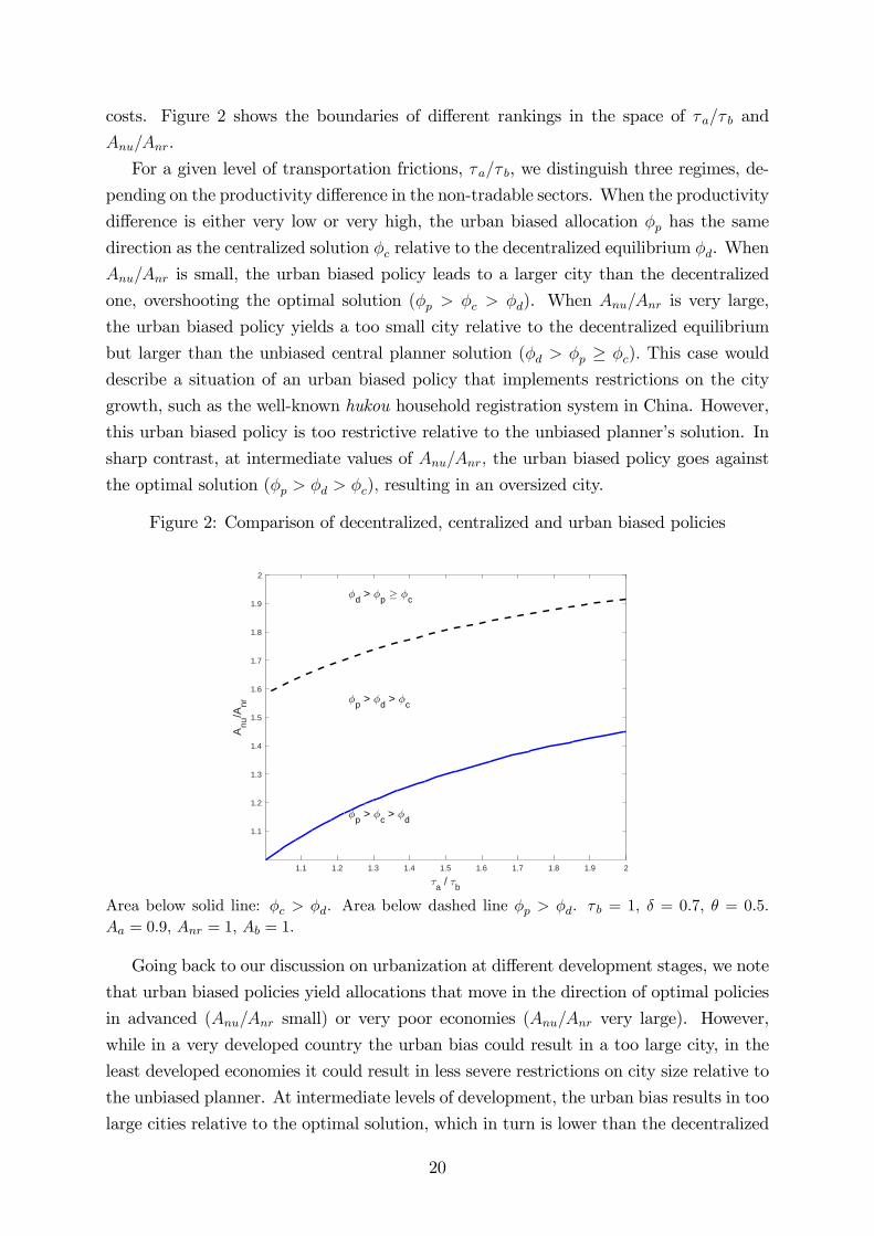
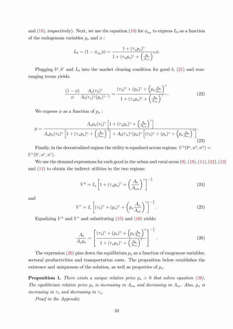
costs. Figure 2 shows the boundaries of different rankings in the space of τa/τ b and
Anu/Anr.
For a given level of transportation frictions, τa/τ b, we distinguish three regimes, de-
pending on the productivity difference in the non-tradable sectors. When the productivity
difference is either very low or very high, the urban biased allocation φp has the same
direction as the centralized solution φc relative to the decentralized equilibrium φd. When
Anu/Anr is small, the urban biased policy leads to a larger city than the decentralized
one, overshooting the optimal solution (φp > φc > φd). When Anu/Anr is very large,
the urban biased policy yields a too small city relative to the decentralized equilibrium
but larger than the unbiased central planner solution (φd > φp ≥ φc). This case would
describe a situation of an urban biased policy that implements restrictions on the city
growth, such as the well-known hukou household registration system in China. However,
this urban biased policy is too restrictive relative to the unbiased planner’s solution. In
sharp contrast, at intermediate values of Anu/Anr, the urban biased policy goes against
the optimal solution (φp > φd > φc), resulting in an oversized city.
Figure 2: Comparison of decentralized, centralized and urban biased policies
1.1 1.2 1.3 1.4 1.5 1.6 1.7 1.8 1.9 2
a /
b
1.1
1.2
1.3
1.4
1.5
1.6
1.7
1.8
1.9
2
Anu
/Anr
p >
c >
d
p >
d >
c
d >
p
c
Area below solid line: φc > φd. Area below dashed line φp > φd. τ b = 1, δ = 0.7, θ = 0.5.Aa = 0.9, Anr = 1, Ab = 1.
Going back to our discussion on urbanization at different development stages, we note
that urban biased policies yield allocations that move in the direction of optimal policies
in advanced (Anu/Anr small) or very poor economies (Anu/Anr very large). However,
while in a very developed country the urban bias could result in a too large city, in the
least developed economies it could result in less severe restrictions on city size relative to
the unbiased planner. At intermediate levels of development, the urban bias results in too
large cities relative to the optimal solution, which in turn is lower than the decentralized
20
city size.
8 Concluding remarks
We study decentralized and optimal urbanization in a simple multi-sector model fo-
cusing on productivity differences and transportation frictions in the context of trade
between urban and rural areas. We show that even in the absence of the typical ex-
ternalities studied in the literature, such as agglomeration, congestion or public goods,
the decentralized city can be either too large or too small relative to that chosen by
a benevolent planner. In particular, optimal urbanization exceeds decentralized levels
when productivity differences in the production of location specific non-traded goods is
small. A numerical exercise calibrated to Brazilian data suggests that the wedges can be
quantitatively important.
Finally, we extend our model to incorporate urban-biased policies. We find that
an urban biased planner will implement a city size that exceeds the optimal one when
productivity differences in non-traded sectors are small, a situation likely to arise in
more developed economies. In contrast, urban biased policies will result in restricted
urbanization in developing economies where these productivity differences tend to be
large.
Our theory uncovers important linkages between the industrial structure of an econ-
omy and the urbanization process and has stark policy implications that depend on the
development stage of an economy. Nonetheless, further research is needed to better un-
derstand these policy implications, in particular by explicitly analyzing how the sector
level productivity and transportation costs interact with the agglomeration and conges-
tion externalities routinely studied in the urbanization literature.
References
Acemoglu, D. and F. Zilibotti (2001). Productivity differences. The Quarterly Journal
of Economics 116 (2), 563—606.
Agnosteva, Delina E., A. J. E. and Y. V. Yotov (2019). Intra-national trade costs:
Assaying regional frictions. European Economic Review 112, 32 —50.
Albouy, D., K. Behrens, F. Robert-Nicoud, and N. Seegert (2018). The optimal distrib-
ution of population across cities. Journal of Urban Economics.
Albrecht, L. and T. Trevor Tombe (2016). Internal trade, productivity, and interconnected
industries: A quantitative analysis. Canadian Journal of Economics 49 (1), 237 —263.
21

Arnott, R. (1979). Optimal city size in a spatial economy. Journal of Urban Eco-
nomics 6 (1), 65 —89.
Atkin, D. and D. Donaldson (2015). Who’s getting globalized? the size and implications
of intra- national trade costs. Technical report.
Beckmann, M. J. (1972). Von thunen revisited: A neoclassical land use model. The
Swedish Journal of Economics 74 (1), 1—7.
Berliant, Marcus, R. R. R. and P. Wang (2006). Knowledge exchange, matching, and
agglomeration. Journal of Urban Economics 60 (1), 69 —95.
Bezemer, D. and D. Headey (2008). Agriculture, development, and urban bias. World
Development 36 (8), 1342 —1364.
Black, D. and V. Henderson (1999). A theory of urban growth. Journal of Political
Economy 107 (2), 252—284.
Carlino, Gerald A., S. C. and R. M. Hunt (2007). Urban density and the rate of invention.
Journal of Urban Economics 61 (3), 389 —419.
Ciccone, A. and R. E. Hall (1996). Productivity and the density of economic activity.
The American Economic Review 86 (1), 54—70.
Costinot, A. and A. Rodriguez-Clare (2014). Chapter 4 - Trade Theory with Numbers:
Quantifying the Consequences of Globalization, Volume 4 of Handbook of International
Economics, pp. 197 —261. Elsevier.
Drazen, A. and Z. Eckstein (1988). On the organization of rural markets and the process
of economic development. The American Economic Review 78 (3), 431—443.
Duarte, M. and D. Restuccia (2019). Relative prices and sectoral productivity. Working
papers, University of Toronto, Department of Economics.
Eaton, J. and Z. Eckstein (1997). Cities and growth: Theory and evidence from france
and japan. Regional Science and Urban Economics 27 (4), 443 —474.
Fan, S. C. and O. Stark (2008). Rural-to-urban migration, human capital, and agglom-
eration. Journal of Economic Behavior and Organization 68 (1), 234 —247.
Frocrain, P. and P.-N. Giraud (2017, May). The evolution of tradable and non-tradable
employment: evidence from France. Working papers, HAL.
Fuller, B. and P. Romer (2014). Urbanization as Opportunity. The World Bank.
22
Gautier, P. A. and C. N. Teulings (2009). Search and the city. Regional Science and
Urban Economics 39 (3), 251 —265.
Gervais, A. and B. J. Jensen (2015). The tradability of services: Geographic concentration
and trade costs, mimeo.
Glaeser, E. L. (1999). Learning in cities. Journal of Urban Economics 46 (2), 254 —277.
Glaeser, E. L. (2014). A world of cities: The causes and consequences of urbanization in
poorer countries. Journal of the European Economic Association 12 (5), 1154—1199.
Glomm, G. (1992). A model of growth and migration. The Canadian Journal of Eco-
nomics 25 (4), 901—922.
Henderson, J. (2010). Will the rural economy rebound in 2010? Economic Review 95 (Q
I), 95—119.
Henderson, J. V. (1974). The sizes and types of cities. The American Economic Re-
view 64 (4), 640—656.
Holmes, T. J. (2005). The location of sales offi ces and the attraction of cities. Journal of
Political Economy 113 (3), 551—581.
Imbs, J., C. Montenegro, and R. Wacziarg (2012). Economic integration and structural
change. Technical report, Political Economy Seminar, Toulouse.
IPUMS (2018). Minnesota population center. integrated public use microdata series,
international: Version 7.1 [dataset]. Technical report, Minneapolis, MN: IPUMS, 2018.
https://doi.org/10.18128/D020.V7.1.
Itoh, R. (2009). Dynamic control of rural-urban migration. Journal of Urban Eco-
nomics 66 (3), 196 —202.
Jensen, B. J. and L. G. Kletzer (2005). Tradable services: Understanding the scope and
impact of services offshoring. Brookings Trade Forum, 75—133.
Kolko, J. (1999). Can i get some service here? information technology, service industries,
and the future of cities.
Lall, Somik V., S. H. and Z. Shalizi (2006). Rural-Urban Migration In Developing Coun-
tries : A Survey Of Theoretical Predictions And Empirical Findings. The World Bank.
Lanjouw, J. O. and P. Lanjouw (2001). The rural non-farm sector: issues and evidence
from developing countries. Agricultural Economics 26 (1), 1—23.
23
Liedholm, C. and D. C. Mead (1987). Small scale industries in developing countries:
Empirical evidence and policy implications. Technical report.
Lipton, M. (1977).Why poor people stay poor : a study of urban bias in world development.
London : Canberra, ACT : Temple Smith ; Australian National University Press.
Lucas, R. E. (1988). On the mechanics of economic development. Journal of Monetary
Economics 22 (1), 3 —42.
Lucas, R. E. (2001). Externalities and Cities. Review of Economic Dynamics 4 (2),
245—274.
Lucas, R. E. (2004). Life earnings and rural?urban migration. Journal of Political Econ-
omy 112 (S1), S29—S59.
Mills, E. S. and D. M. de Ferranti (1971). Market choices and optimum city size. The
American Economic Review 61 (2), 340—345.
Ott, I. and S. Soretz (2010). Productive public input, integration and agglomeration.
Regional Science and Urban Economics 40 (6), 538 —549.
Poelhekke, S. and F. Van der Ploeg (2008). Globalization and the rise of mega-cities in
the developing world. Technical report.
Porter, M. E., C. K. K. M. and R. Bryden (2004). Competitiveness in rural u.s. regions:
Learning and research agenda. Technical report.
Reardon, Thomas, B. J. and G. Escobar (2001). Rural nonfarm employment and incomes
in latin america: Overview and policy implications. World Development 29 (3), 395 —
409.
Sheshinski, E. (1973). Congestion and the optimum city size. The American Economic
Review 63 (2), 61—66.
The World Urbanization Prospects (2018). The World Urbanization Prospects 2018.
United Nations Department of Economic and Social Affairs, Population Division,
United Nations.
Wiggins, S. and S. Proctor (2001). How special are rural areas? the economic implications
of location for rural development. Development Policy Review 19 (4), 427—436.
Yang, D. T. (1999). Urban-biased policies and rising income inequality in china. American
Economic Review 89 (2).
24
A Appendix A
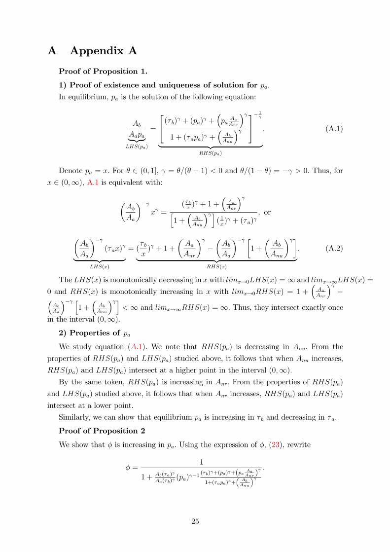
Proof of Proposition 1.
1) Proof of existence and uniqueness of solution for pa.In equilibrium, pa is the solution of the following equation:
AbAapa︸ ︷︷ ︸LHS(pa)
=
(τ b)γ + (pa)γ +(pa
AaAnr
)γ1 + (τapa)γ +
(AbAnu
)γ−
1γ
︸ ︷︷ ︸RHS(pa)
. (A.1)
Denote pa = x. For θ ∈ (0, 1], γ = θ/(θ − 1) < 0 and θ/(1 − θ) = −γ > 0. Thus, forx ∈ (0,∞), A.1 is equivalent with:
(AbAa
)−γxγ =
( τbx)γ + 1 +
(AaAnr
)γ[1 +
(AbAnu
)γ]( 1x)γ + (τa)γ
, or
(AbAa
)−γ(τax)
γ︸ ︷︷ ︸LHS(x)
= (τ bx)γ + 1 +
(AaAnr
)γ−(AbAa
)−γ [1 +
(AbAnu
)γ]︸ ︷︷ ︸
RHS(x)
. (A.2)
The LHS(x) is monotonically decreasing in x with limx→0LHS(x) =∞ and limx→∞LHS(x) =
0 and RHS(x) is monotonically increasing in x with limx→0RHS(x) = 1 +(AaAnr
)γ−(
AbAa
)−γ [1 +
(AbAnu
)γ]<∞ and limx→∞RHS(x) =∞. Thus, they intersect exactly once
in the interval (0,∞).2) Properties of pa
We study equation (A.1). We note that RHS(pa) is decreasing in Anu. From the
properties of RHS(pa) and LHS(pa) studied above, it follows that when Anu increases,
RHS(pa) and LHS(pa) intersect at a higher point in the interval (0,∞).By the same token, RHS(pa) is increasing in Anr. From the properties of RHS(pa)
and LHS(pa) studied above, it follows that when Anr increases, RHS(pa) and LHS(pa)
intersect at a lower point.
Similarly, we can show that equilibrium pa is increasing in τ b and decreasing in τa.
Proof of Proposition 2
We show that φ is increasing in pa. Using the expression of φ, (23), rewrite
φ =1
1 + Ab(τa)γ
Aa(τb)γ(pa)γ−1
(τb)γ+(pa)γ+(pa AaAnr)γ
1+(τapa)γ+(AbAnu
)γ.
25

Denote pa = x and f(x) = Ab(τa)γ
Aa(τb)γxγ−1
(τb)γ+xγ+(x Aa
Anr)γ
1+(τax)γ+(AbAnu
)γ . Thus,∂φ
∂x= − ∂f/∂x
(1 + f(x))2, (A.3)
where
∂f/∂x = (γ − 1)f(x)x
+f(x)γxγ−1
[1 +
(AaAnr
)γ](τ b)γ + (x)γ +
(x AaAnr
)γ − γf(x)(τa)γxγ−1
1 + (τax)γ +(
AbAnu
)γ , or
∂f/∂x = (γ − 1)f(x)x
+ f(x)γxγ−1
[1 +
(AaAnr
)γ] [1 +
(AbAnu
)γ]− (τa)γ(τ b)γ[
(τ b)γ + (x)γ +(x AaAnr
)γ] [1 + (τax)γ +
(AbAnu
)γ] .As (τa)γ(τ b)γ < 1 and γ < 0, then
[1 +
(AaAnr
)γ] [1 +
(AbAnu
)γ]− (τa)γ(τ b)γ > 0.
As γ − 1 = 1/(θ − 1) < 0 for θ < 1, then ∂f(x)/∂x < 0. Consequently, ∂φ/∂x > 0.Proof of Proposition 3.
In order to prove existence of an interior solution in the interval (0, 1), we study the
properties of welfare function when φ→ 0 and φ→ 1.
The aggregate welfare function is:
W (φ) = φV u(φ) + (1− φ)V r(φ),
where
V u(φ) = Ab
[1 + (τapa(φ))
γ +
(AbAnu
)γ]− 1γ
V r(φ) = Aapa(φ)
[(τ b)
γ + (pa(φ))γ +
(pa(φ)
AaAnr
)γ]− 1γ
= Aa
[(τ b
pa(φ)
)γ+ 1 +
(AaAnr
)γ]− 1γ
,
and pa(φ) is given by (22).
Step 1. We study limφ→0W (φ) and limφ→1W (φ).
We study the first term of W (φ), φV u(φ) and second term (1− φ)V r(φ) when φ→ 0
and φ→ 1.
26

Using (23), the first term φV u(φ) can be written as:
AaAbpa(τ b)γ[1 + (τapa)
γ +(
AbAnu
)γ] γ−1γAapa(τ b)γ
[1 + (τapa)γ +
(AbAnu
)γ]+ Ab(τa)γ(pa)γ
[(τ b)γ + (pa)γ +
(pa
AaAnr
)γ] orAaAb(τ b)
γ(pa)γ[(pa)
−γ + (τa)γ + (pa)
−γ(
AbAnu
)γ] γ−1γAa(pa)1+γ(τ b)γ
[(pa)−γ + (τa)γ + (pa)−γ
(AbAnu
)γ]+ Ab(τa)γ(pa)2γ
[(pa)−γ(τ b)γ + 1 +
(AaAnr
)γ] orAaAb(τ b)
γ[(pa)
−γ + (τa)γ + (pa)
−γ(
AbAnu
)γ] γ−1γAapa(τ b)γ
[(pa)−γ + (τa)γ + (pa)−γ
(AbAnu
)γ]+ Ab(τa)γ(pa)γ
[(pa)−γ(τ b)γ + 1 +
(AaAnr
)γ] .From equation (23) we can see that φ→ 0 when pa → 0, and φ→ 1 when pa →∞.When pa → 0, (pa)
−γ → 0 and (pa)γ →∞ as γ < 0. Thus limφ→0 φVu(φ) = 0.
When pa →∞, (pa)γ → 0 as γ < 0. Thus limφ→1 φVu(φ) =
AaAb(τb)γ[1+(AbAnu
)γ] γ−1γAa(τb)γ
[1+(AbAnu
)γ]+Ab(τa)γ(pa)γ−1(τb)γ
=
Ab
[1 +
(AbAnu
)γ]− 1γ
> 0.
The second term of W (φ), (1− φ)V r(φ) is rewritten as:
AaAb(τa)γ(pa)
γ+1[(τ b)
γ + (pa)γ +
(pa
AaAnr
)γ]1− 1γ
Aapa(τ b)γ[1 + (τapa)γ +
(AbAnu
)γ]+ Ab(τa)γ(pa)γ
[(τ b)γ + (pa)γ +
(pa
AaAnr
)γ] orAaAb(τa)
γ(pa)2γ[(pa)
−γ(τ b)γ + 1 +
(AaAnr
)γ]1− 1γ
Aa(pa)1+γ(τ b)γ[(pa)−γ + (τa)γ + (pa)−γ
(AbAnu
)γ]+ Ab(τa)γ(pa)2γ
[(pa)−γ(τ b)γ + 1 +
(AaAnr
)γ] orAaAb(τa)
γ[(pa)
−γ(τ b)γ + 1 +
(AaAnr
)γ]1− 1γ
Aa(pa)1−γ(τ b)γ[(pa)−γ + (τa)γ + (pa)−γ
(AbAnu
)γ]+ Ab(τa)γ
[(pa)−γ(τ b)γ + 1 +
(AaAnr
)γ] .When pa → 0, (pa)
−γ → 0 and (pa)1−γ → 0 as γ < 0. Thus limφ→0(1 − φ)V r(φ) =
Aa
[1 +
(AaAnr
)γ]− 1γ
> 0.
When pa →∞, (pa)γ → 0 as γ < 0. Thus,
limφ→1(1− φ)V r(φ) = AaAb(τa)γ(pa)γ [(τb)
γ ]1− 1
γ
Aa(τb)γ[1+(AbAnu
)γ]+Ab(τa)γ(pa)γ−1(τb)γ
= 0.
Thus, limφ→0W (φ) = Aa
[1 +
(AaAnr
)γ]− 1γ
> 0 and limφ→1W (φ) = Ab
[1 +
(AbAnu
)γ]− 1γ
>
0.
Step 2. We study limφ→0 ∂W (φ)/∂φ and limφ→1 ∂W (φ)/∂φ.
∂W (φ)
∂φ= V u(φ) + φ
∂V u(φ)
∂φ− V r(φ) + (1− φ)∂V
r(φ)
∂φ
27

First, we rewrite ∂W (φ)/∂φ as:
Ab
[1 + (τapa)
γ +
(AbAnu
)γ]− 1γ
− φAb[1 + (τapa)
γ +
(AbAnu
)γ]− 1γ−1
(τa)γ(pa)
γ−1∂pa(φ)
∂φ
−paAa[(τ b)
γ + (pa)γ +
(paAaAnr
)γ]− 1γ
+ (1− φ)Aa[(τ b)
γ + (pa)γ +
(paAaAnr
)γ]− 1γ ∂pa(φ)
∂φ
−(1− φ)Aa(pa)γ[(τ b)
γ + (pa)γ +
(paAaAnr
)γ]− 1γ−1∂pa(φ)
∂φ
[1 +
(AaAnr
)γ].
Further rearranging terms, we obtain ∂W (φ)/∂φ =:
Ab
[1 + (τapa)
γ +
(AbAnu
)γ]− 1γ
︸ ︷︷ ︸g1(φ)
− φAb[1 + (τapa)
γ +
(AbAnu
)γ]− 1γ−1
(τa)γ(pa)
γ−1∂pa(φ)
∂φ︸ ︷︷ ︸g2(φ)
−paAa[(τ b)
γ + (pa)γ +
(paAaAnr
)γ]− 1γ
︸ ︷︷ ︸g3(φ)
+ (1− φ)Aa(τ b)γ[(τ b)
γ + (pa)γ +
(paAaAnr
)γ]− 1γ−1∂pa(φ)
∂φ︸ ︷︷ ︸g4(φ)
.
Next, we calculate ∂pa(φ)/∂φ, which we will use to evaluate the limits of g2(φ) and
g4(φ).
According to the implicit function theorem:
∂pa(φ)
∂φ= − ∂Z/∂φ
∂Z/∂pa,
where Z = (1−φ)φ
Aa(τb)γ
Ab(τa)γ(pa)γ−1− (τb)
γ+(pa)γ+(pa AaAnr)γ
1+(τapa)γ+(AbAnu
)γ . Furthermore:
∂Z
∂φ= − 1
φ2Aa(τ b)
γ
Ab(τa)γ(pa)γ−1,
∂Z
∂pa=(1− φ)φ
Aa(τ b)γ(1− γ)
Ab(τa)γ(pa)γ+γ(τa)
γ(pa)γ−1(τ b)
γ + (pa)γ +
(pa
AaAnr
)γ[1 + (τapa)γ +
(AbAnu
)γ]2−γ(pa)γ−1[1 +
(AaAnr
)γ]1 + (τapa)γ +
(AbAnu
)γ .We rewrite the second and third term in ∂Z/∂pa using the fact that Z = 0. Thus,∂Z∂pa
= (1−φ)φ
Aa(τb)γ(1−γ)
Ab(τa)γ(pa)γ+ (1−φ)
φAa(τb)
γ
Ab(τa)γ(pa)γ−1γ(τa)γ(pa)γ−1
1+(τapa)γ+(AbAnu
)γ− (1−φ)φ
Aa(τb)γ
Ab(τa)γ(pa)γ−1γ(pa)γ−1[1+( AaAnr
)γ]
(τb)γ+(pa)γ+(pa AaAnr)γ
28

= (1−φ)φ
Aa(τb)γ
Ab(τa)γ(pa)γ−1
[1−γpa+ γ(τa)γ(pa)γ−1
1+(τapa)γ+(AbAnu
)γ − γ(pa)γ−1[1+( AaAnr)γ]
(τb)γ+(pa)γ+(pa AaAnr)γ
].
∂pa(φ)
∂φ=
φ(1− φ)(pa)γ−11− γ(pa)γ
+γ(τa)
γ
1 + (τapa)γ +(
AbAnu
)γ − γ[1 +
(AaAnr
)γ](τ b)γ + (pa)γ +
(pa
AaAnr
)γ
−1
.
(A.4)
We proceed in two steps.
A. We study limφ→0 ∂W (φ)/∂φ. When φ → 0, (pa)γ → ∞, therefore limφ→0 g1(φ) =
∞ and
limφ→0 g3(φ) = limφ→0Aa
[(τ b)
γ(pa)−γ + 1 +
(AaAnr
)γ]− 1γ
= Aa
[1 +
(AaAnr
)γ]− 1γ
.
Using the expression (A.4), we can write g2(φ) as:
Ab(τa)γ
[1 + (τapa)
γ +
(AbAnu
)γ]− 1γ−1
(1− φ)−1 ×1− γ(pa)γ
+γ(τa)
γ(pa)γ−1
1 + (τapa)γ +(
AbAnu
)γ − γ(pa)γ−1[1 +
(AaAnr
)γ](τ b)γ + (pa)γ +
(paAaAnr
)γ−1 or
Ab(τa)γ(pa)
−1−γ[(pa)
−γ + (τa)γ + (pa)
−γ(AbAnu
)γ]− 1γ−1
(1− φ)−1 ×
×
1− γ(pa)γ
+ γ(pa)−γ−1
(τa)γ(τ b)
γ −[1 +
(AbAnu
)γ] [1 +
(AaAnr
)γ][(pa)−γ + (τa)γ + (pa)−γ
(AbAnu
)γ] [(τ b)γ(pa)−γ + 1 +
(AaAnr
)γ]−1 or
Ab(τa)γ
[(pa)
−γ + (τa)γ + (pa)
−γ(AbAnu
)γ]− 1γ−1
(1− φ)−1 ×
×
(1− γ)pa + γ(τa)
γ(τ b)γ −
[1 +
(AbAnu
)γ] [1 +
(AaAnr
)γ][(pa)−γ + (τa)γ + (pa)−γ
(AbAnu
)γ] [(τ b)γ(pa)−γ + 1 +
(AaAnr
)γ]−1 .
Thus, limφ→0 g2(φ) = 0.
29

Next, we write g4(φ) as:
Aa(τ b)γ
[(τ b)
γ + (pa)γ +
(paAaAnr
)γ]− 1γ−1
φ−1(pa)γ+1 ×
×
(1− γ)pa + γ(τa)
γ(τ b)γ −
[1 +
(AbAnu
)γ] [1 +
(AaAnr
)γ][(pa)−γ + (τa)γ + (pa)−γ
(AbAnu
)γ] [(τ b)γ(pa)−γ + 1 +
(AaAnr
)γ]−1 or
Aa(τ b)γ
[(τ b)
γ(pa)−γ + 1 +
(AaAnr
)γ]− 1γ−1
φ−1 ×
×
(1− γ)pa + γ(τa)
γ(τ b)γ −
[1 +
(AbAnu
)γ] [1 +
(AaAnr
)γ][(pa)−γ + (τa)γ + (pa)−γ
(AbAnu
)γ] [(τ b)γ(pa)−γ + 1 +
(AaAnr
)γ]−1
We can see that limφ→0 g4(φ) =∞. Thus limφ→0 ∂W (φ)/∂φ =∞.B. We study limφ→1 ∂W (φ)/∂φ. When φ → 1, (pa)
γ → 0, therefore limφ→1 g1(φ) =
Ab
[1 +
(AbAnu
)γ]− 1γ
,
limφ→1 g3(φ) =∞ and limφ→1 g4(φ) = 0. Finally, we write g2(φ) as:
Ab(τa)γ
[1 + (τapa)
γ +
(AbAnu
)γ]− 1γ−1
(1− φ)−1(pa)γ ×
×
1− γ + γ(pa)−1
(τa)γ(τ b)
γ −[1 +
(AbAnu
)γ] [1 +
(AaAnr
)γ][1 + (τapa)γ +
(AbAnu
)γ] [(τ b)γ + (pa)γ +
(paAaAnr
)γ]−1 .
We calculate
limφ→1(1−φ)−1(pa)γ = limφ→1Aapa(τb)
γ[1+(τapa)γ+
(AbAnu
)γ]+Ab(τa)
γ(pa)γ[(τb)γ+(pa)γ+(pa AaAnr)γ]
Ab(τa)γ[(τb)γ+(pa)γ+(pa AaAnr)γ]
=
∞.Thus, limφ→1 g2(φ) =∞. We conclude that limφ→0 ∂W (φ)/∂φ = −∞.SinceW (φ) is differentiable on the interval (0, 1), these properties ensure the existence
of an interior welfare maximum.
Proof of Proposition 4.
We compare pa(φd) to Ab/Aa. When φ = φd, the relative price pa satisfies the utility
equalization condition (A.2) studied in Proposition 1.
We evaluate the LHS(pa) and RHS(pa) of this expression at pa = Ab/Aa to check
when pa(φd) < Ab/Aa or vice-versa.
LHS(AbAa
)= (τa)
γ and
RHS(AbAa
)= (τ b)
γ(AbAa
)−γ+ 1 +
(AaAnr
)γ−(AbAa
)−γ [1 +
(AbAnu
)γ]When pa(φd) < Ab/Aa, LHS
(AbAa
)< RHS
(AbAa
), as LHS(pa) is decreasing over
(0,∞) and RHS(pa) is increasing.
30

The condition is (τa)γ < (τ b)γ(AbAa
)−γ+ 1 +
(AaAnr
)γ−(AbAa
)−γ [1 +
(AbAnu
)γ], or
(τa)γ(Aa)
−γ < (τ b)γ (Ab)
−γ + (Aa)−γ + (Anr)
−γ −[(Ab)
−γ + (Anu)−γ] .
Rearranging terms, we obtain:
(Anu)−γ − (Anr)−γ < (Aa)−γ [1− (τa)γ]− (Ab)−γ [1− (τ b)γ] .
If the condition above holds, then AbAa
> pa and ∂W∂φ
∣∣∣φ=φd
> 0, so planner wants a
larger city, i.e. φc > φd.
The opposite holds when RHS(AbAa
)< LHS
(AbAa
). Then, ∂W
∂φ
∣∣∣φ=φd
< 0, so the
planner wants a smaller city, φc < φd.
Proof of Proposition 6.
We evaluate the sign of ∂W p
∂φ
∣∣∣φ=φd
. If ∂W p
∂φ
∣∣∣φ=φd
, then φp > φd, where φp is the solution
of ∂Wp
∂φ= 0.
∂W p(φ)
∂φ
∣∣∣∣φ=φd
=
[δV u(φ) + φδ
∂V u(φ)
∂φ− (1− δ)V r(φ) + (1− δ)(1− φ)∂V
r(φ)
∂φ
]∣∣∣∣φ=φd
.
∂W p
∂φ
∣∣∣∣φ=φd
= φd∂V u(φ)
∂φ
∣∣∣∣φ=φd
+ (1− φd)∂V r(φ)
∂φ
∣∣∣∣φ=φd
(A.5)
= −V r(φd)(1− φd)(pa)γ−1
(τ b)γ + (pa)γ +(pa
AaAnr
)γ [1 + ( AaAnr
)γ]∂pa(φ)
∂φ
∣∣∣∣φ=φd
+ V r(φd)(1− φd)
pa
∂pa(φ)
∂φ
∣∣∣∣φ=φd
− V u(φd)φd(pa)
γ−1(τa)γ
1 + (τapa)γ +(
AbAnu
)γ ∂pa(φ)
∂φ
∣∣∣∣φ=φd
,
As V u(φd) = V r(φd), we can write∂W p(φ)∂φ
∣∣∣φ=φd
as
[φδ∂V u(φ)
∂φ+ (1− δ)(1− φ)∂V
r(φ)
∂φ
]∣∣∣∣φ=φd
+ (2δ − 1)V u(φd)
= V u(φd)
−δφd
(τa)γ(pa)γ−1
1+(τapa)γ+(AbAnu
)γ−−(1− δ)(1− φd)
[1+( AaAnr)γ](pa)γ−1
(τb)γ+(pa)γ+(pa AaAnr)γ + (1− δ)(1− φd) 1pa
∂pa(φ)
∂φ
∣∣∣∣φ=φd
+(2δ − 1)V u(φd).
Rearranging terms, we obtain ∂W p
∂φ
∣∣∣φ=φd
as:
31

V u(φd)
−δφd(τa)γ(pa)γ−1
1+(τapa)γ+(AbAnu
)γ+(1− δ)(1− φd) 1
(pa)(τb)
γ
(τb)γ+(pa)γ+(pa AaAnr)γ
∂pa(φ)
∂φ
∣∣∣∣φ=φd
+ (2δ − 1)V u(φ), or
V u(φd)(pa)γ−1
1 + (τapa)γ +(
AbAnu
)γ︸ ︷︷ ︸
D>0
−δφd(τa)γ
+(1− δ)(1− φd)(τb)
γ
(pa)γ
1+(τapa)γ+(AbAnu
)γ(τb)γ+(pa)γ+(pa Aa
Anr)γ
∂pa(φ)
∂φ
∣∣∣∣φ=φd
+ (2δ − 1)V u(φ)
We use the fact that φd satisfies the utility equalization condition:(1−φd)φd
Aa(τb)γ
Ab(τa)γ(pa)γ−1=
(τb)γ+(pa)γ+(pa Aa
Anr)γ
1+(τapa)γ+(AbAnu
)γ .
We obtain:
∂W p
∂φ
∣∣∣∣φ=φd
=δDφd(τa)
γ
pa
{(1− δδ
AbAa− pa(φd)
}∂pa(φ)
∂φ
∣∣∣∣φ=φd
+ (2δ − 1)V u(φ).
As 2δ − 1 > 0, a suffi cient condition for ∂W p
∂φ
∣∣∣φ=φd
> 0 is 1−δδ
AbAa− pa(φd) > 0.
We use the fact that pa(φd) satisfies the utility equalization condition (A.2).(AbAa
)−γ(τax)
γ︸ ︷︷ ︸LHS(x)
= (τ bx)γ + 1 +
(AaAnr
)γ−(AbAa
)−γ [1 +
(AbAnu
)γ]︸ ︷︷ ︸
RHS(x)
We evaluate the LHS(pa) and RHS(pa) of this expression at (1− δ)Ab/δAa to checkwhen pa(φd) < (1− δ)Ab/δAa.
LHS(1−δδ
AbAa
)=(1−δδ
)−γ(τa)
γ and
RHS(1−δδ
AbAa
)= (τ b)
γ(1−δδ
AbAa
)−γ+ 1 +
(AaAnr
)γ−(AbAa
)−γ [1 +
(AbAnu
)γ]LHS(pa) is decreasing over (0,∞) and RHS(pa) is increasing. Thus, when pa(φd) <
(1− δ)Ab/δAa,LHS
(1−δδ
AbAa
)< RHS
(1−δδ
AbAa
).
The condition is (τa)γ(1−δδ
)−γ< (τ b)
γ(1−δδ
AbAa
)−γ+1+
(AaAnr
)γ−(AbAa
)−γ [1 +
(AbAnu
)γ].
Denote κ = (1− δ)/δ < 1, when δ > 1/2. The condition above becomes:(τa)
γ(κAa)−γ < (τ b)
γ (κAb)−γ + (Aa)
−γ + (Anr)−γ −
[(Ab)
−γ + (Anu)−γ] .
Rearranging terms, we obtain:
(Anu)−γ − (Anr)−γ < (Aa)−γ
[1− (κ/τa)−γ
]− (Ab)−γ
[1− (κ/τ b)−γ
].
(Anu)−γ − (Anr)−γ < (Aa)−γ − (Ab)−γ + κ−γ
[(Abτ b
)−γ−(Aaτa
)−γ].
32

When pa(φd) < (1− δ)Ab/δAa, then ∂W p
∂φ
∣∣∣φ=φd
> 0. Thus, φp > φd.
When δ ∈ (1/2, 1), (1 − δ)Ab/δAa < Ab/Aa. When pa(φd) < Ab/Aa, ∂W c
∂φ
∣∣∣φ=φd
> 0
and thus φc > φd.
33