Call Me Educated 27aug2015 - sites.tufts.edu · In rural areas of developing countries, public worker absence – of teachers, doctors, nurses or agricultural extension agents –

“Call Me Educated: Evidence from a Mobile Monitoring Experiment in Niger”

Jenny C. Aker and Christopher Ksoll

May 2015

Abstract. In rural areas of developing countries, education programs are often implemented through community teachers. While teachers are a crucial part of the education production function, observing their effort remains a challenge for the public sector. This paper tests whether a simple monitoring system, implemented via the mobile phone, can improve student learning as part of an adult education program. Using a randomized control trial in 160 villages in Niger, we randomly assigned villages to a mobile phone monitoring component, whereby teachers, students and the village chief were called on a weekly basis. There was no incentive component to the program. The monitoring intervention dramatically affected student performance: During the first year of the program, reading and math test scores were .15-.30 s.d. higher in monitoring villages than in non-monitoring villages, with relatively stronger effects in the region where monitoring was weakest and for teachers for whom the outside option was lowest. We provide more speculative evidence on the mechanisms behind these effects, namely, teacher and student effort and motivation. JEL codes: D1, I2, O1, O3

*Jenny C. Aker, The Fletcher School and Department of Economics, Tufts University, 160 Packard Avenue, Medford, MA 02155; [email protected]. Christopher Ksoll, School of International Development and Global Studies, University of Ottawa, 120 University, Ottawa, ON, Canada; [email protected]. We thank Michael Klein, Julie Schaffner, Shinsuke Tanaka and seminar participants at Tufts University, the Center for Global Development and IFPRI for helpful comments. We thank Melita Sawyer for excellent research assistance. We are extremely grateful for funding from the DFID Economic and Social Research Council (Grant Number ES/L005433/1).

In rural areas of developing countries, public worker absence – of teachers, doctors,

nurses or agricultural extension agents – is a widespread problem. In West Africa,

teacher absenteeism is estimated between 27-40%. Despite numerous interventions to

overcome the monitoring problem, such as community-based monitoring, “para-

teachers”, audits or other incentives, teacher monitoring continues to be a significant

challenge. This is particularly the case in countries with limited infrastructure and weak

institutions, where the costs of monitoring are particular high.

The introduction of mobile phone technology throughout sub-Saharan Africa has

the potential to reduce the costs associated with monitoring public employees, such as

teachers. By allowing governments and organizations to communicate with remote

villages on a regular basis, “mobile monitoring” has the potential to increase the

observability of the agents’ effort. Similarly, reductions in communication costs

associated with mobile phone technology could potentially increase community

engagement in the monitoring process, thereby providing the community with additional

bargaining power.

We report the results of a randomized monitoring intervention in Niger, where a

mobile phone monitoring component was added to an adult education program.

Implemented in 160 villages in two rural regions of Niger, students followed a basic adult

education curriculum, but half of the villages also received a monitoring component –

weekly phone calls to the teacher, students and village chief. No other incentives or

formal sanctions were provided in the short-term.

Overall, our results provide evidence that the mobile phone monitoring

substantially improved learning outcomes. Adults’ reading and math test scores were

0.15–0.30 standard deviations (SD) higher in the mobile monitoring villages immediately

after the program, with a statistically significant impact. These effects were relatively

higher in one region where monitoring was more difficult and were also stronger for

teachers for whom the outside option was lowest. These effects do not appear to be

driven by differential attrition or differences in teacher quality, but are partially explained

by increased teacher effort and motivation, as well as some increased student motivation.

Our finding that monitoring leads to an improvement in skills acquisition

contributes to a debate on the effectiveness of education monitoring in other contexts.

Using monitoring and financial incentives randomized experiment in India – specifically

using cameras -- Duflo, Hanna and Ryan (2012) find that teacher absenteeism fell by 21

percentage points and children’s test scores increased by 0.17 s.d. Using a nationally

representative dataset of schools in India, Muralidharan et al (2014) find that increased

school monitoring is strongly correlated with lower teacher absence, but do not measure

effects on learning. Using mobile phone monitoring linked to financial incentives,

Cilliers et al (2014) find that the introduction of financial incentives increased teacher

attendance and monitoring frequency, but similarly do not measure impacts upon

learning. Our experiment is somewhat unique in that it did not provide any explicit

financial incentives.1

The remainder of the paper is organized as follows. Section II provides

background on the setting of the research and the research design, whereas Section III

presents the model. Section IV describes the different datasets and estimation strategy,

and Section V presents the results. Section VI addresses the potential mechanisms and 1 Our paper also contributes to the literature on community-based monitoring and inspection systems (Svensson 2007, Olken 2007, Bengtsson and Engstrom 2014).

Section VII discusses alternative explanations. Section VIII discusses cost-benefit

analyses and Section IX concludes.

II. Research Setting and Experimental Design With a gross national income per capita of $641, Niger is one of the lowest-ranked

countries on the UN’s Human Development (UNDP 2014). The country has some of the

lowest educational indicators in sub-Saharan Africa, with estimated literacy rates of 15

percent in 2012 (World Bank 2015). Illiteracy is particularly striking among women and

within our study region: It is estimated that only 10 percent of women attended any

school in the Maradi and Zinder regions.

A. Adult Education and Mobile Monitoring Interventions

Starting in March 2014, an international non-governmental organization (NGO),

Catholic Relief Services, implemented an adult education program in two rural regions of

Niger. The intervention provided five months of literacy and numeracy instruction over a

to approximately 25,000 adults across 500 villages. Courses were held between March

and July, with a break between July and January due to the agricultural planting and

harvesting season. All classes taught basic literacy and numeracy skills in the native

language of the village (Hausa), as well as functional literacy topics on health, nutrition

and agriculture. Conforming to the norms of the Ministry of Non-Formal Education,

each village had two literacy classes (separated by gender), with 35 women and 15 men

per class. Classes were held five days per week for three hours per day, and were taught

by community members who were selected and trained in the adult education

methodology by the Ministry of Non-Formal Education.2

The mobile monitoring component was implemented in a subset of the adult

education villages. For this intervention, data collection agents made four weekly phone

calls over a six-week period, calling the literacy teacher, the village chief and two

randomly selected students (one female and one male). No phones were provided to

either teachers or students. 3 During the phone calls, the field agents asked if the class

was held in the previous week, how many students attended and why classes were not

held.4 The mobile monitoring component was introduced two months after the start of

the adult education program, and neither students, teachers, nor CRS field staff were

informed of which villages were selected prior to the calls.

While general information on the results of the monitoring calls were shared with

CRS on a weekly basis, due to funding constraints, neither CRS nor the Ministry were

able to conduct additional monitoring visits. In fact, the overall number of monitoring

visits was extremely low for all villages in 2014. In addition, teachers were not formally

sanctioned for less than contracted effort during the first year of the intervention; rather,

2 Unlike previous adult education programs in Niger, the same teacher taught both classes in the village. In addition, the differences in class size by gender makes it difficult for us to disentangle the learning effects by gender as compared with differences in the class size. 3Phone numbers for the students were obtained during the initial registration phase for the program. If the student’s household did not have a phone, the number of a friend or family member was obtained, and this person was called to reach the student. For the first year, the same two students were called over the six-week period. 4Two field agents made four calls per village per week for six weeks. They followed a short script and then asked five questions: Was there a literacy course this week? How many days per week? How many hours per day? How many students attended? Is there anything else you would like to share?

teachers only learned whether they would be retained for the second year well after the

end of classes.5

B. Experimental Design

In 2013, CRS identified over 500 intervention villages across two regions of

Niger, Maradi and Zinder. Of these, we randomly sampled 160 villages as part of the

research program. Among these 160 villages, we first stratified by regional and sub-

regional administrative divisions. Villages were then randomly assigned to the adult

education program (to start classes in 2014) or a comparison group (to start classes in

2016). Among the adult education villages, villages were then assigned to either the

monitoring or no monitoring intervention. In all, 140 villages were assigned to the adult

education program and 20 villages were assigned to the pure control group.6 Among the

adult education villages, 70 villages were assigned to monitoring and 70 to the no

monitoring condition.7 A map of the project areas is provided in Figure 1, and a timeline

of the implementation and data collection activities is provided in Figure 2.

Within each village, CRS identified eligible students in both the adult education

and comparison villages prior to the baseline. Individual-level eligibility was determined

by two primary criteria: illiteracy (verified by an informal writing test) and willingness to

participate in the adult education program. 5 While CRS did have a policy for modifying salaries based upon attendance, as well as firing teachers after the first year, in practice, no formal sanctions for less than contracted effort were immediately applied: no one was fired, pay was not reduced, no follow-up visits, etc. 6While we only have 20 villages in the control group, our power calculations were based upon previous research in Niger on adult education outcomes. Aker, Ksoll and Lybbert (2012) find that a mobile phone-enhanced adult education program increased writing and math test scores by .20-.25 s.d. as compared with a traditional adult education program. The simple unreported and non-experimental before-after comparison of the traditional adult education program in Aker et al. (and the basis of the power calculations for this paper) suggested a much larger effect size of over 5 s.d. as compared with the baseline scores. With this effect size a sample of 20 villages in the control group was largely sufficient to determine the causal impact of the adult education intervention. 7 In 2015, half of the villages will receive the ABC program, a mobile phone module.

II. Model

A simple conceptual framework provides some intuition as to how monitoring

might affect teachers’ effort and student learning. A principal (the NGO or government)

hires a short-term contractual teacher to teach an adult education program, but is unable

to obtain complete information about the teachers’ effort, related to imperfect

supervision. Assuming that teachers believe they may be fired or penalized, monitoring

should increase teachers’ effort, which can vary with the intensity of monitoring and the

cost of being fired.

Suppose that the NGO hires adult education teachers at a wage rate, wNGO.

Teachers can choose to exert some effort: e=1 (non-shirker) or e=0 (shirker). For

simplicity, there are only two effort levels. Teachers who exert some effort will remain

employed by the NGO for the duration of their contract. However, those who exert zero

effort (shirkers) risk being caught (and fired) probability θ. These teachers can find a

new job with probability pm and receive an outside wage wm, which requires effort em.

Using this framework, the utility function for shirkers and non-shirkers is

therefore:

(1) UNS = wNGO eUS = (1 )wNGO + pm(wm em )

In order to extract positive levels of effort from the teachers, the NGO will choose a wage

rate which assures that UNS ≥ US, or that the non-shirking condition is satisfied:

(2) 𝑤 ≥ 𝑝 (𝑤 − 𝑒 ) +

There can be a positive correlation between the teacher’s effort (e) and the NGO

wage rate (wNGO), but testing this empirically is impossible since effort cannot be

verified. The higher the teacher’s outside option (outside wage net effort), the less likely

he or she is to accept the NGO wage offer.8 Assuming that the teacher accepts the

NGO’s offer, the teacher will then choose effort to maximize his/her expected utility.

Outside wage rates can vary by individual (wim), as it might be more likely for

teachers with outside experience to find a job or more likely for male teachers to find

jobs, as women are traditionally restricted to the local labor market. This will modify the

non-shirker’s utility function (slightly) to an individual-specific one, US,i. This suggests

that the NGO should tailor the wage and monitoring to the teacher’s outside options, but

in practice, the NGO can only set a single wage, which will not satisfy the non-shirking

condition for every teacher. As a result, a proportion of the teachers will shirk.

A mobile phone monitoring intervention affects the teacher’s probability of being

caught and fired θ, so that 𝜃 ∈ (𝜃 , 𝜃 ), where L corresponds to the default (low

monitoring) state and H to the additional mobile phone monitoring. This leads to the

following modifications:

(3) UNS = wNGO eUS,i = (1 T )wNGO + T pm(wm

i em )

Thus, the optimal 𝑤 ∗ for which the teacher is indifferent between working and shirking

will depend upon the level of monitoring. Again, since the NGO cannot set an

individual-specific wage rate, a proportion 𝜏(𝑤 , 𝜃) of teachers will shirk.

Student learning outcomes are characterized by the following education

production function: 8 In theory the NGO has two tools at its disposal to ensure teachers exert effort, namely wNGO and θ, and the optimal combination of the two will be the outcome of the NGO's optimization process, including the cost of monitoring. Unless the wage is chosen such that no one shirks, the exact levels will not change any of our following results

(4) 𝑦 = 𝑦(𝑒 ) 𝑦(0)𝑖𝑓 𝑒 = 0𝑦(1)𝑖𝑓 𝑒 = 1

where 𝑒 is the effort exerted by student i's teacher, and teacher effort positively affects

learning outcomes. This model does not show complementarities or substitutes between

teacher and student effort. The average student outcome will therefore be a function of

the share of teachers providing effort:

(5) 𝑦 = 𝜏 𝑦(0) + (1 − 𝜏 )𝑦(1)

This leads to the following predictions with mobile phone monitoring:

x Prediction 1. As the probability of getting fired rises (θT), then < 0, so >

0. This is true whenever the NGO wage is greater than the outside wage net

effort option, but this needs to be the case for teachers to accept the post in the

first place. Since student achievement rises in student effort, then > 09

x Prediction 2. If the attractiveness of the teacher’s outside option rises, i.e. pm or

(wim- em) rises, then the consequences of shirking become less severe and the

proportion of teachers providing effort goes down: i.e. > 0 and ( )

>

0. This implies that students’ learning outcomes will decrease with the

attractiveness of teachers' outside options, so that < 0.10

IV. Data and Estimation Strategy

9 Cueto et al. (2008) show that the relationship between teacher attendance and achievement may be non-linear. In other words, in the beginning, an increase in teacher attendance led to an increase in student achievement; however, there was a point at which higher teacher attendance no longer led to further improvements in student achievement. 10 This is not necessarily true when pm(wi

m-em) and teacher ability are correlated, as then a higher ability teacher might still teach better even when shirking. Then locally, the above result holds, but not when you change outside options in a discrete way. At this point the fact that we have measures of teacher ability become important. Conditional on ability the above results hold.

The data we use in this paper come from three primary sources. First, we

conducted individualized math and reading tests and use these scores to measure the

impact of the program on educational outcomes. Second, we implemented household-

level surveys. Third, we collected administrative and survey data on teachers, and use

these data to better understand the mechanisms behind the effects. Before presenting our

estimation strategy, we discuss each of these data sources in detail.

A. Test Score and Self-Esteem Data

Our NGO partner identified students in all villages and for all cohorts in January

2014. While we had originally intended to implement the baseline in all 160 villages, the

delayed start of the adult education program during the first year, as well as delays in

funding, meant that we were only able to conduct the baseline in a subset of the sample

(91 villages).11 In these villages, we stratified students by gender and took a random

sample of 16 students per village. We implemented reading and math tests prior to the

start of courses (February 2014), providing a baseline sample of approximately 1,271

students. We administered follow-up tests in the same baseline villages (91) as well as a

random sample of non-baseline villages (30 villages) in August 2014, thereby allowing

us to estimate the immediate impacts of the program. This total sample was 1,926

students, excluding attrition.

To test students’ reading and math skills, we used USAID’s Early Grade Reading

Assessment (EGRA) and Early Grade Math Assessment (EGMA) tests. These are a

series of individual tasks in reading and math, often used in primary school programs.

EGRA is a series of timed tests that measure basic foundational skills for literacy

11To choose the baseline villages, we stratified by region, sub-region and treatment status and selected a random sample of villages for the baseline. We also used a similar process to add on the 30 villages for the first follow-up survey.

acquisition: recognizing letters, reading simple words and phrases and reading

comprehension. Each task ranges from 60-180 seconds; if the person misses four

answers in a row, the exercise is stopped. EGMA measures basic foundational skills for

math acquisition: number recognition, comparing quantities, word problems, addition,

subtraction, multiplication and division.

The EGRA and EGMA tests were our preferred survey instruments, as compared

with the Ministry’s standard, untimed battery of writing and math tests, for two reasons.

First, most adult education programs are criticized for high rates of skills’ depreciation.

Yet these high rates of skills’ depreciation may be simply due to the levels of reading

achieved by the end of traditional adult education programs, which are often not captured

in traditional untimed tests. For example, the short-term memory required to store

deciphered material is brief, lasting 12 seconds and storing 7 items (Abadzi 2003). Thus,

“Neoliterates must read a word in about 1-1.5 second (45-60 words per minute) in order

to understand a sentence within 12 seconds (Abadzie 2003).”12 Thus, the EGRA timed

tests allow us to determine whether participants in adult education classes are attaining

the threshold required for sustained literacy acquisition. Second, the tests offer a great

detail of precision in terms of skills acquisition, capturing more nuanced levels of

variation in learning.

During the reading and math tests, we also measured students’ self-esteem and

self-efficacy, as measured by the Rosenberg Self-Esteem Scale (RSES) and the General

Self-Efficacy Scale (GSES). The RSES is a series of statements designed to capture

different aspects of self-esteem (Rosenberg 1965). Five of the statements are positively

12This speed corresponds to oral-reading U.S. norms for first grade children. However, this is often not attained in literacy classes. For example, studies in Burkina Faso indicate that most literacy graduates need 2.2 seconds to read a word and are correct only 80-87 percent of the time (Abadzi 2003).

worded, while the other five statements are negatively-worded. Each answer is assigned

a point value, with higher scores reflecting higher self-esteem. The GSES is a ten-item

psychometric scale that is designed to assess whether the respondent believes he or she is

capable of performing new or difficult tasks and to deal with adversity in life (Schwarzer

and Jerusalem 1995). The scale ranges in value from 12-60, with higher scores reflecting

higher perceived self-efficacy. We use these results to measure the impact of the

program on participants’ perceptions of empowerment.

Attrition is typically a concern in adult education classes. Table A1 formally tests

whether there is differential attrition by treatment status for the follow-up survey round.

Average dropout in the comparison group was 5 percent, with relatively higher drop-out

in the adult education classes (without monitoring) and lower dropout in the adult

education classes (with monitoring). Thus, drop-out was relatively higher in the adult

education group as compared with the comparison group, but the monitoring program

might have prevented student drop-out. Non-attriters in the adult education villages were

more likely to be female as compared with non-attriters in the comparison villages,

although there were no statistically significant differences among other characteristics

between the monitoring and non-monitoring villages. The former difference would likely

bias our treatment effect downwards, as female students have lower test scores as

compared with male students in adult education classes (Aker et al 2012).

B. Household Survey Data

The second primary dataset includes information on baseline household

characteristics. We conducted a baseline household survey in February 2014 with 1,271

adult education students across 91 villages, the same sample as those for the test score

data. The survey collected detailed information on household demographics, assets,

production and sales activities, access to price information, migration and mobile phone

ownership and usage. These data are primarily used to test for balance imbalances across

the different treatments, as well as to test for heterogeneous effects.

C. Teacher Data

The third dataset is comprised of teacher-level characteristics and motivation.

Using administrative data from CRS’ teacher screening and training process, the dataset

includes information on teachers’ level of education, age, gender and village residence.

In addition, in November 2014, we conducted a survey of all teachers in adult education

villages, which included an intrinsic motivation test and teachers’ perceptions of the

monitoring program.

C. Pre-Program Balance

Table 1A suggests that the randomization was successful in creating comparable

groups along observable dimensions. Differences in pre-program household

characteristics are small and insignificant (Table 1, Panel A). Average age was 34, and a

majority of respondents were members of the Hausa ethnic group. The average education

level of household members was 2 years. Fifty-eight percent of households in the sample

owned a mobile phone, with 61 percent of respondents having used a mobile phone in the

months prior to the baseline. Respondents primarily used the mobile phone to make and

receive calls. All respondents reporting receiving calls (as compared with making calls),

as making a phone call requires being able to recognize numbers on the handset. While

some baseline characteristics are statistically significant – such as asset and mobile phone

ownership, which are related -- overall, we made over 100 baseline comparisons across

the treatment groups and find statistically significant differences that are consistent with

what one would expect of randomization.

Table 1B provides further evidence of the comparability across the treatments for

reading scores. Using non-normalized baseline reading scores for each task, students in

comparison villages had low levels of letter, syllable, word or phrase recognition prior to

the program, without a statistically significant between the treatment and control groups

or between the monitoring and non-monitoring villages. Comparisons of baseline math

scores (Table 1C), similarly suggest comparability across the different groups, with the

exception of one math task. This suggests that the project successfully selected

participants who were illiterate and innumerate prior to the start of the program.

Table 1D presents a comparison of teacher characteristics across the adult

education villages. Overall teacher characteristics are well-balanced between the

monitoring and non-monitoring villages. Teachers were 37 years old and approximately

37 percent had some secondary education. Roughly one-third of the teachers were

female, and a strong majority were married.

D. Estimation Strategy To estimate the impact of both the adult education program and monitoring on

educational outcomes, we use a simple differences specification. Let testiv be the reading

or math test score attained by student i in village v immediately after the program.

adultedv is an indicator variable for whether the village v is assigned to the adult

education intervention (adulted=1) or the control (adulted=0). adulated*monitort takes

on the value of one if the adult education village received the mobile monitoring

intervention, and 0 otherwise. θR are geographic fixed effects at the regional and sub-

regional levels (the level of stratification). 𝐗 is a vector of student-level baseline

covariates, primarily gender, although we include the baseline test score in some

specifications. We estimate the following specification:

(6) 𝑡𝑒𝑠𝑡 = 𝛽 + 𝛽 𝑎𝑑𝑢𝑙𝑡𝑒𝑑 + 𝛽 𝑎𝑑𝑢𝑙𝑡𝑒𝑑 ∗ 𝑚𝑜𝑛𝑖𝑡𝑜𝑟 + 𝑋 + 𝜃 + 𝜀 The coefficients of interest is are β1 and β2, which capture the average immediate impact

of the adult education program (without monitoring) and the additional impact of the

mobile phone monitoring program. The error term εiv captures unobserved student ability

or idiosyncratic shocks. We cluster the error term at the village level for all

specifications.

Equation (6) is our preferred specification. As an alternative to this preferred

approach, we also estimate the impact of the program using a value-added specification

and difference-in-differences, the latter of which allows us to control for village-level

fixed effects. However, these reduce our sample size, as we do not have baseline data

for all villages.

V. Results Figures 3A and 3B depict the mean normalized reading and math test scores for

the adult education villages with and without monitoring immediately after the end of

classes. Test scores are normalized using the mean and s.d. of contemporaneous test

scores in comparison villages. The means of the comparison group are not shown for

ease of exposition. Three things are worth noting. First, the adult education program

seems to increase reading and math scores significantly as compared to the comparison

group, with relatively stronger effects on reading (although no one achieved the

“threshold” reading level). Second, these effects are also stronger for “lower level” tasks,

i.e., simple letter or syllable recognition and addition and subtraction. And third, the

difference in test scores between monitoring and non-monitoring villages is almost

equivalent to the difference in test scores between the non-monitoring villages and the

comparison group, especially for lower-level tasks. This suggests powerful learning

gains from the monitoring program.

A. Immediate Impact of the Program

Table 2 presents the results of Equation (3) for reading test scores. Across all

reading tasks, the adult education program increased students’ reading test scores by .12-

.27 s.d., with a statistically significant effect at the 5 percent level for reading letters and

syllables (Table 2, Panel A, Columns 1 and 2) and the composite score (Column 5).

These adult education impacts are relatively stronger in Maradi (Panel C) as compared to

Zinder (Panel B). Overall, the monitoring component increased reading test scores by

.14-.30 s.d., with a statistically significant effect at the 5 and 10 percent levels across all

reading measures. These results are primarily driven by villages in Zinder (Panel B), the

region with the lowest achievement gains for the adult education program and with a

larger geographic area over which to conduct monitoring.

The results are similar, although with a lower magnitude, for math (Table 3): the

adult education program increased math z-scores by .08-.23 s.d. (Panel B, Column 1),

with a statistically significant effect at the 5 and 10 percent levels. These results are

primarily stronger in the Maradi region (Panel C). Overall, the monitoring component

increased test scores by .08-.15 s.d., although the statistically significant effects are

primarily for simpler math tasks (Panel A) and for the Zinder region (Panel B). The

results in Table 3 are also robust to using value-added specifications, the latter of which

controls for average baseline test scores at the village level.

A key interest in adult education programs is whether such programs affect

student empowerment. We therefore measure the impact of the adult education program

and the mobile monitoring component on self-esteem and self-efficacy, using the RSES

and GSES (Table 4). Overall, self-esteem and self-efficacy scores were 2-3 percent

lower in the adult education as compared to control villages, although only with a

statistically significant effect for self-efficacy scores (Table 4, Panel A). These effects

are relatively stronger in the Zinder region, where students achieved the lowest literacy

gains (Panel B). The monitoring component seems to mitigate this effect: monitoring

villages have higher levels of self-efficacy as compared with students in the non-

monitoring adult education villages.

While potentially surprising, this seems to mirror the results found in Ksoll et al

(2014), who found that students’ perceptions of self-esteem changed over time,

particularly when they experienced learning failures. Since students in the Zinder region

attained lower levels of learning overall, they could have potentially felt less capable in

the short-term, although the monitoring component mitigated this effect.

B. Heterogeneous Effects of the Program We would expect greater learning benefits among certain subpopulations, such as

men and women, or according to teachers’ characteristics, as predicted by our model.

Table 5 tests for heterogeneous impacts of the program by the student’s gender, while

Table 6 tests for heterogeneous effects by teacher characteristics, in particular proxies for

outside options.

In light of different socio-cultural norms governing women’s and men’s

household responsibilities and social interactions, the adult education and monitoring

program could have different impacts by gender. As women of particular ethnic groups

(e.g., the Hausa) travel outside of their home village less frequently than men, the adult

education classes may have provided fewer opportunities for women to practice outside

of class, thereby weakening their incentives to learn. In addition, given the differences in

class size between men and women, women could have been disadvantaged by the larger

student-to-teacher ratio. Table 5 presents the results by gender. On average, women’s

reading and math z-scores were lower than men’s immediately after the program, similar

to the results found in Aker et al (2012). The monitoring component had a stronger

impact on men’s reading test scores as compared with women’s, even though teachers

taught both courses.

Table 6 presents these results by teachers’ characteristics, namely gender,

education level (secondary or below) and previous experience as an adult education

teacher. In many villages in the Maradi and Zinder regions of Niger, women often do not

migrate, and therefore have more localized and constrained labor market options.

Teachers with higher levels of education should have higher outside options, thereby

reducing the effectiveness of monitoring component. The results suggest that this is the

case: While monitoring increases reading and math z-scores of adult education students

regardless of the teacher characteristics, with relatively stronger impacts on reading, the

impact of monitoring is stronger for female teachers and those with less experience,

consistently with our model. As for teachers with less experience, monitoring is less

effective for new teachers, primarily for reading. This suggests that newer teachers might

have had better outside options.

VI. Potential Mechanisms

There are a variety of mechanisms through which the monitoring component

could affect students’ learning. First, mobile monitoring can potentially lead to increased

teacher effort, thereby improving the effectiveness of the overall adult education

curriculum. Second, as the phone calls could potentially increase teachers’ intrinsic

motivation, thereby increasing their teaching efficacy and the impact of the program.

Third, having a more present and motivated teacher could potentially affect students’

effort, leading to increased class participation and attendance. And finally, as the

monitoring component involved students, the calls could have motivated students

independently, who in turn motivated their fellow learners. While we have more

speculative evidence on each of these, we present evidence on each of these mechanisms

in turn.

A. Teacher Effort and Motivation

The mobile phone monitoring could have increased teacher effort within the

classroom, thereby improving students’ performance. As we are unable to directly

observe teacher effort, we assess the impact on a self-reported proxy. CRS and the

Ministry of Non-Formal Education provided norms for the number of classes to be taught

during each month, yet the actual number of classes taught was at the discretion of each

teacher. While we would prefer an external, objective measure of the number of classes’

taught, for the short-term, we use teachers’ self-reported measures of whether or not they

stopped the class and the number of days stopped. Table 7 shows the results of the

monitoring component on teachers’ self-reported effort and measures of intrinsic

motivation. Overall, while teachers in monitoring villages were not less likely to stop the

course at any point during the curriculum, they reported suspending the course for 1.27

fewer days, with a statistically significant difference at the 10 percent level (Panel A).

This suggests that the observed improvements in test scores may have been due to

increased duration of the course, although the margin of this effect is quite small. This is

in part supported by qualitative data: Teachers reported that “The…calls prevent us from

missing courses”, and that “Someone who works must be ‘controlled’”. However, there

was no correlation between monitoring and the teacher’s likelihood of being replaced

between the first and second year (Panel C).

In addition to affecting the duration of courses, the calls could have affected

teachers’ intrinsic motivation, thereby making them more effective in class. Teachers

themselves reported that the calls “prove that our work is important” and that they gave

them “courage”. While monitoring did not appear to have an impact on an index of self-

reported pressure, perceived competence or choice, it did appear to increase motivation,

as measured by a 10-point scale: teachers reported feeling more interested in the task,

with a statistically significant effect at the 10 percent level (Table 7, Panel B). However,

with only 140 observations, we may be underpowered to detect small effects.

B. Student Effort and Motivation The monitoring component could have encouraged greater student effort within

the classes, as measured by student attendance or motivation. While we do not have

reliable data on student attendance, we do have measures of student dropout at some

point during the course and the reason for drop-out. Table 8 shows these results.

Overall, the monitoring component did not appear to affect the likelihood of student

dropout (Table 8, Panel A) nor the likelihood of a student dropping out for an

endogenous reason (i.e., lack of time, lack of interest) as opposed to an exogenous shock

(pregnancy, illness, death in the family).

Nevertheless, there is some suggestive evidence that the monitoring component

affected student learning via the mechanism of calling students themselves. Panel B

shows the results of a regression of test scores on a binary variable for students who were

called, as well as the monitoring treatment and an interaction term between the two.

While the “called” students only represents 8 percent of the total sample, the calls

appeared to affect students’ learning: called students had significantly higher reading and

math z-scores as compared with non-called students in monitoring villages, as well as

students in non-monitoring villages. It is possible that the called students’ greater

motivation passed to other students, although we cannot test this hypothesis.13

VII. Alternative Explanations

There are two potential confounds to interpreting the above findings. First, there

might be differential in-person monitoring between monitoring and non-monitoring

villages. If the Ministry of Non-Formal Education or CRS decided to focus more of their

efforts on monitoring villages because they had better information, then any differences

we observe in test scores might be due to differences in program implementation, rather

than the monitoring component. Yet during the first year of the program, there was very

little in-person monitoring, and no differential visits by treatment status.

13 The main results are robust to excluding the “called” students from the sample, although the magnitudes of the coefficients are smaller (Table A5).

A second potential confounding factor could be due to differential attrition. The

results in Table A1 suggest that attrition is higher in the adult education villages as

compared with the comparison group and lower in the monitoring villages (as compared

with non-monitoring villages). While it is difficult to predict the potential direction of

this bias, we use Lee bounds to correct for bias for differential attrition between the

monitoring and non-monitoring villages, our primary comparison of interest. Table A2

suggests that the upper bounds remain positive and statistically significant

(unsurprisingly), and that the lower bounds for reading and math test scores are still

positive and statistically significant for most of the primary outcomes.

Finally, as we are conducting a number of comparisons across multiple outcomes,

there is a risk that our results could be due to probabilistic equivalence, at least in part.

Using a Bonferroni correction accounting for family-wise correlation, we modify the p-

values to account for these multiple comparisons, with the results in Table A3. Overall,

the results are robust for the reading outcomes and for those in the Zinder region.14

VIII. Cost-Effectiveness

A key question is the cost-effectiveness of the mobile intervention as compared to

regular monitoring. While in-person monitoring visits were limited in the context of the

first year of the study, we have data on per-monitoring costs for both in-person and

mobile monitoring (Figure 4). On average, in-person monitoring costs are $13 per

village, as compared with $6.5. This suggests that per-village savings are $6.5, as

compared with average gains of .20 s.d. in learning.

14 The small number of observations in the control group could raise concerns that are confidence intervals are too narrow (Cameron, Gelbach and Miller 2008). We therefore re-estimate our core results while using a bootstrap-t procedure for our standard errors (Table A4) and find similar results.

IX. Conclusion

Adult education programs are an important part of the educational system in many

developing countries. Yet the successes of these initiatives have been mixed, partly due

to the appropriateness of the educational input and the ability of governments and

international organizations to monitor teachers’ effort. How to improve learning in these

contexts is not clear.

This paper assesses the impact of an intervention that conducted mobile

monitoring of an adult education intervention. We find that this substantially increased

students’ skills acquisition in Niger, suggesting that mobile telephones could be a simple

and low-cost way to improve adult educational outcomes. The treatment effects are

striking: the adult education program with monitoring increased reading and math test

scores by .15-.25 s.d. as compared with the standard adult education program. The

impacts appear to operate through increasing teacher effort and motivation, although we

are unable to clearly identify the precise mechanism at this time.

References Abadzi, Helen. 1994. "What We Know About Acquisition of Adult Literacy: Is There

Hope?," In World Bank discussion papers,, ix, 93 p. Washington, D.C.: The World Bank.

Abadzi, Helen. 2013. Literacy for All in 100 Days? A research-based strategy for fast

progress in low-income countries," GPE Working Paper Series on Learning No. 7 Aker, Jenny C., Christopher Ksoll and Travis J. Lybbert. October 2012. “Can

Mobile Phones Improve Learning? Evidence from a Field Experiment in Niger.” American Economic Journal: Applied Economics. Vol 4(4): 94-120.

Andrabi, Tahir, Jishnu Das, Asim Ijaz Khwaja, and Tristan Zajonc. 2011. "Do

Value-Added Estimates Add Value? Accounting for Learning Dynamics." American Economic Journal: Applied Economics, 3(3): 29–54.

Angrist, Joshua D., and Jorn - Steffen Pischke. 2009. Mostly Harmless Econometrics: Banerjee, Abhijit, Shawn Cole, Esther Duflo and Leigh Linden. 2007. "Remedying

Education: Evidence from Two Randomized Experiments in India." The Quarterly Journal of Economics, 122(3), pp. 1235-64.

Banerji, Rukmini, James Berry and Marc Shotland. 2013. "The Impact of Mother

Literacy and Participation Programs on Child Learning: A Randomized Evaluation in India."

Barrow, Lisa, Lisa Markman and Cecilia Elena Rouse. 2009. "Technology's Edge:

The Educational Benefits of Computer-Aided Instruction." American Economic Journal: Economic Policy, 1(1), pp. 52-74.

Blunch, Niels-Hugo and Claus C. Pörtner. 2011. "Literacy, Skills and Welfare: Effects

of Participation in Adult Literacy Programs." Economic Development and Cultural Change. Vol. 60, No. 1 (October 2011): 17-66.

Cameron, A. Colin, Jonah B. Gelbach, and Douglas L. Miller. 2008. "Bootstrap-

based improvements for inference with clustered errors." Review of Economics and Statistics 90.3: 414-427.

Carron, G. 1990. "The Functioning and Effects of the Kenya Literacy Program." African

Studies Review, pp. 97-120. Cilliers, Jacobus, Ibrahim Kasirye, Clare Leaver, Pieter Serneels,and Andrew

Zeitlin. 2014. “Pay for locally monitored performance? A welfare analysis for teacher attendance in Ugandan primary schools.”

DiNardo, J., J. McCrary, and L. Sanbonmatsu. 2006. "Constructive Proposals for Dealing with Attrition: An Empirical Example." Working paper, University of Michigan.

Duflo, Esther, Rema Hanna and Stephen Ryan. 2012. “Incentives Work: Getting

Teachers to Come to School,” American Economic Review. Duflo, Esther. 2012. "Women Empowerment and Economic Development." Journal of

Economic Literature. 50(4). 1051-1079. Doepke, Mathias and Michele Tertilt. 2014. "Does Female Empowerment Promote

Economic Development?" NBER Working Paper 19888, NBER, Inc. Lee, David S. 2009. “Training, Wages, and Sample Selection: Estimating Sharp Bounds

on Treatment Effects” The Review of Economic Studies, 6, 1072-1102. Muralidharan, Karthik, Jishnu Das, Alaka Holla and Aakash Mohpal. 2014. “The

Fiscal Cost of Weak Governance: Evidence from Teacher Absence in India.” Unpublished mimeo.

Ortega, Daniel and Francisco Rodríguez. 2008. "Freed from Illiteracy? A Closer Look

at Venezuela’s Mision Robinson Literacy Campaign." Economic Development and Cultural Change, 57, pp. 1-30.

Osorio, Felipe, and Leigh L. Linden. 2009. "The use and misuse of computers

in education: evidence from a randomized experiment in Colombia." The World Bank Policy Research Working Paper Series.

Oxenham, John, Abdoul Hamid Diallo, Anne Ruhweza Katahoire, Anne Petkova-

Mwangi and Oumar Sall. 2002. Skills and Literacy Training for Better Livelihoods: A Review of Approaches and Experiences. Washington D.C.: World Bank.

Romain, R. and L. Armstrong. 1987. Review of World Bank Operations in Nonformal

Education and Training. World Bank, Education and Training Dept., Policy Division.

UNESCO. 2005. Education for All: Global Monitoring Report. Literacy for Life. Paris:

UNESCO. UNESCO. 2008. International Literacy Statistics: A Review of Concepts, Methodology

and Current Data. Montreal: UNESCO Institute for Statistics. UNESCO. 2012. Education for All: Global Monitoring Report. Youth and Skills: Putting

Education to Work. Paris: UNESCO.

Table 1A. Baseline Household Characteristics

(1) (2) (3) (4) (5) (6)

Comparison Group Monitoring Adult Educ. Difference Difference p-value

Mean (s.d.) Mean (s.d.) Mean (s.d.) Coeff (s.e) Coeff (s.e.)

Household Characteristics at Baseline (2)-(1) (3)-(1) (2)=(3) Age of Respondent 35.6 33.44 34.08 -1.26 -1.97 0.73

(12.98) (11.63) (12.01) (1.083) (1.273)

Gender of Respondent (1=Female, 0=Male) 0.685 0.677 0.683 0.01 -0.01 0.40

(0.466) (0.468) (0.465) (0.0121) (0.0217)

Average education level of household (in years) 1.787 2.112 2.069 0.12 -0.08 0.19

(0.963) (1.028) (0.985) (0.0811) (0.0906)

Number of asset categories owned by household 5.585 5.895 5.81 0.22* -0.15 0.16

(1.543) (1.6) (1.569) (0.115) (0.206)

Household experienced drought in past year (0/1) 0.471 0.564 0.537 0.03 0.02 0.83

(0.501) (0.496) (0.499) (0.0400) (0.0611)

Household owns a mobile phone (0/1) 0.58 0.685 0.665 0.07** 0.00 0.33

(0.496) (0.465) (0.472) (0.0339) (0.0519)

Respondent used a cell phone since the last harvest 0.61 0.647 0.644 0.03 0.03 0.95

(0.502) (0.478) (0.479) (0.0330) (0.0577)

Used cellphone in past two weeks to make calls 0.737 0.722 0.703 0.04 -0.05 0.25

(0.446) (0.449) (0.457) (0.0338) (0.0591)

Used cellphone in past two weeks to receive calls 1 0.967 0.965 0.00 -0.05*** 0.19 (0) (0.178) (0.185) (0.0165) (0.0227)

Note: This table shows the difference in means between the different treatment groups. "Comparison" is defined as villages assigned to no adult education treatment in 2014 or 2015. "Adult education" is defined as those villages that were assigned to adult education without monitoring, whereas "Monitoring" is defined as villages that were assigned to adult education with monitoring. Standard deviations are shown in parentheses. Columns (4) and (5) show the coefficients and s.e. from a regression of each characteristic on the treatments and stratification fixed effects. Huber-White standard errors clustered at the village level are provided in parentheses. *** significant at the 1 percent level, ** significant at the 5 percent level, * significant at the 10 percent level.

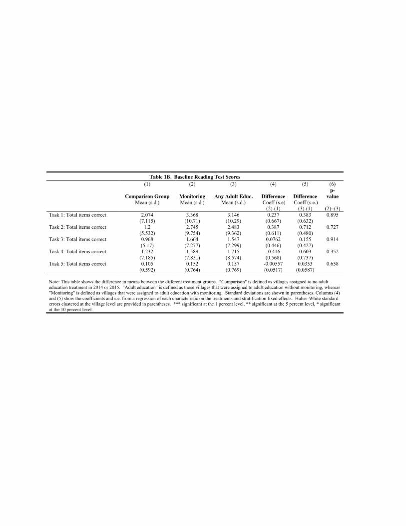
Table 1B. Baseline Reading Test Scores

(1) (2) (3) (4) (5) (6)

Comparison Group Monitoring Any Adult Educ. Difference Difference

p-value

Mean (s.d.) Mean (s.d.) Mean (s.d.) Coeff (s.e) Coeff (s.e.)

(2)-(1) (3)-(1) (2)=(3) Task 1: Total items correct 2.074 3.368 3.146 0.237 0.383 0.895

(7.115) (10.71) (10.29) (0.667) (0.632)

Task 2: Total items correct 1.2 2.745 2.483 0.387 0.712 0.727

(5.532) (9.754) (9.362) (0.611) (0.480)

Task 3: Total items correct 0.968 1.664 1.547 0.0762 0.155 0.914

(5.17) (7.277) (7.299) (0.446) (0.427)

Task 4: Total items correct 1.232 1.589 1.715 -0.416 0.603 0.352

(7.185) (7.851) (8.574) (0.568) (0.737)

Task 5: Total items correct 0.105 0.152 0.157 -0.00557 0.0353 0.658 (0.592) (0.764) (0.769) (0.0517) (0.0587)


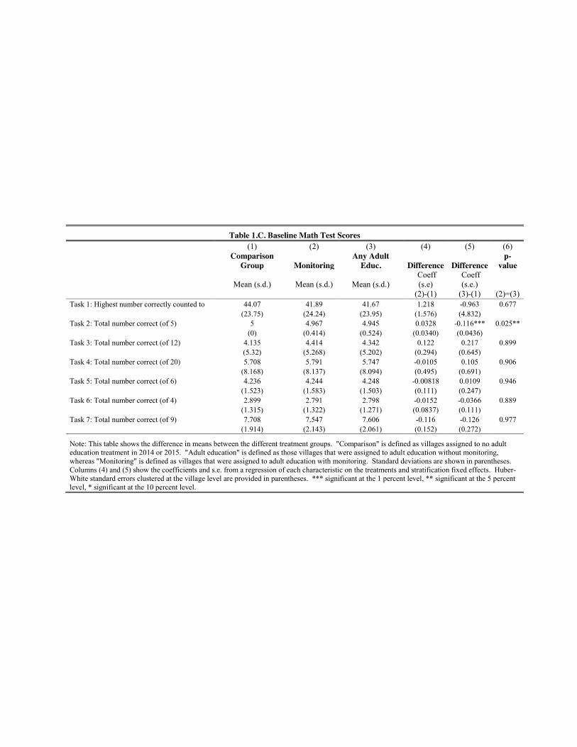
Table 1.C. Baseline Math Test Scores

(1) (2) (3) (4) (5) (6)

Comparison Group Monitoring

Any Adult Educ. Difference Difference

p-value

Mean (s.d.) Mean (s.d.) Mean (s.d.)

Coeff (s.e)

Coeff (s.e.)

(2)-(1) (3)-(1) (2)=(3) Task 1: Highest number correctly counted to 44.07 41.89 41.67 1.218 -0.963 0.677

(23.75) (24.24) (23.95) (1.576) (4.832)

Task 2: Total number correct (of 5) 5 4.967 4.945 0.0328 -0.116*** 0.025**

(0) (0.414) (0.524) (0.0340) (0.0436)

Task 3: Total number correct (of 12) 4.135 4.414 4.342 0.122 0.217 0.899

(5.32) (5.268) (5.202) (0.294) (0.645)

Task 4: Total number correct (of 20) 5.708 5.791 5.747 -0.0105 0.105 0.906

(8.168) (8.137) (8.094) (0.495) (0.691)

Task 5: Total number correct (of 6) 4.236 4.244 4.248 -0.00818 0.0109 0.946

(1.523) (1.583) (1.503) (0.111) (0.247)

Task 6: Total number correct (of 4) 2.899 2.791 2.798 -0.0152 -0.0366 0.889

(1.315) (1.322) (1.271) (0.0837) (0.111)

Task 7: Total number correct (of 9) 7.708 7.547 7.606 -0.116 -0.126 0.977 (1.914) (2.143) (2.061) (0.152) (0.272)


Table 1D. Balance Table of Teacher Characteristics

(1) (2) (3)

Comparison Schools

Adult Education

Only

Adult Education + Monitoring

p-value (1)=(2)

p-value (1)=(3)

p-value (2)=(3)

Panel A. Teacher Characteristics Mean s.d Mean s.d. Mean s.d. Teacher Age

37.35 (8.67) 36.84 (9.37)

0.836

Teacher is female

0.33 (0.47) 0.34 (0.48)

0.816 Teacher is married

0.88 (0.33) 0.92 (0.27)

0.561

Teacher has some secondary education 0.35 (0.48) 0.39 (0.49) 0.569 Note: This table shows the difference in means between the different treatment groups. "Comparison" is defined as villages assigned to no adult education treatment in 2014 or 2015. "Adult education" is defined as those villages that were assigned to adult education without monitoring, whereas "Monitoring" is defined as villages that were assigned to adult education with monitoring. Standard deviations are shown in parentheses. Columns (4) and (5) show the coefficients and s.e. from a regression of each characteristic on the treatments and stratification fixed effects. Huber-White standard errors clustered at the village level are provided in parentheses. *** significant at the 1 percent level, ** significant at the 5 percent level, * significant at the 10 percent level.

Table 2. Reading Timed Z-Scores

(1) (2) (3) (4) (5)

Letters Syllables Words Phrases Composite Score

Panel A: All Villages (1) Adult education 0.27*** 0.22** 0.12 0.13 0.23**

(0.10) (0.10) (0.08) (0.09) (0.10)

(2) Adult education*monitor 0.18* 0.30** 0.14* 0.14* 0.18**

(0.09) (0.13) (0.08) (0.08) (0.09)

Strata fixed effects Yes Yes Yes Yes Yes Observations 1,766 1,766 1,773 1,772 1,791 R-squared 0.02 0.01 0.01 0.01 0.02 Total effect: Adult Education + Monitoring

p-value (Adult education + monitor=0) .00*** .00*** .00*** 0.00*** 0.00*** Panel B: Zinder

(1) Adult education 0.17 0.10 0.04 0.05 0.10

(0.13) (0.14) (0.10) (0.10) (0.12)

(2) Adult education*monitor 0.22* 0.45* 0.19* 0.18* 0.24*

(0.14) (0.22) (0.11) (0.11) (0.14)

Strata fixed effects Yes Yes Yes Yes Yes Observations 898 903 901 898 898 R-squared 0.02 0.01 0.02 0.01 0.02 Total effect: Adult Education + Monitoring

p-value (Adult education + monitor=0) 0.00*** 0.03** 0.05** 0.06* 0.00*** Panel C: Maradi

(1) Adult education 0.44*** 0.37*** 0.25* 0.27* 0.40**

(0.15) (0.13) (0.14) (0.15) (0.16)

(2) Adult education*monitor 0.15 0.17 0.09 0.11 0.15

(0.12) (0.14) (0.11) (0.12) (0.13)

Strata fixed effects Yes Yes Yes Yes Yes Observations 875 875 875 875 875 R-squared 0.02 0.01 0.01 0.01 0.02 Total effect: Adult Education + Monitoring

p-value (Adult education + monitor=0) 0.000 0.001 0.05 0.03 0.001

Notes: This table presents the results from a regression of different reading outcomes on adult education (only), adult education plus monitoring and randomization fixed effects. Huber-White standard errors clustered at the village level are provided in parentheses. *** significant at the 1 percent level, ** significant at the 5 percent level, * significant at the 10 percent level.

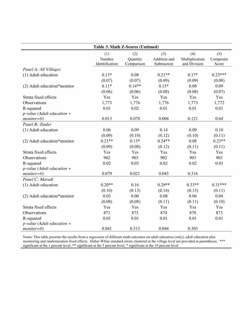
Table 3. Math Z-Scores (Untimed)

(1) (2) (3) (4) (5)

Number Identification

Quantity Comparison

Addition and Subtraction

Multiplication and Division

Composite Score

Panel A: All Villages (1) Adult education 0.13* 0.08 0.21** 0.17* 0.23***

(0.07) (0.07) (0.09) (0.09) (0.08)

(2) Adult education*monitor 0.11* 0.14** 0.15* 0.08 0.09

(0.06) (0.06) (0.08) (0.08) (0.07)

Strata fixed effects Yes Yes Yes Yes Yes Observations 1,773 1,776 1,776 1,773 1,772 R-squared 0.01 0.02 0.01 0.01 0.01 p-value (Adult education + monitor=0) 0.013 0.078 0.004 0.121 0.64 Panel B: Zinder

(1) Adult education 0.06 0.09 0.14 0.09 0.10

(0.09) (0.10) (0.12) (0.10) (0.11)

(2) Adult education*monitor 0.21** 0.13* 0.24** 0.08 0.23**

(0.09) (0.08) (0.12) (0.11) (0.11)

Strata fixed effects Yes Yes Yes Yes Yes Observations 902 903 902 903 903 R-squared 0.02 0.03 0.02 0.02 0.03 p-value (Adult education + monitor=0) 0.079 0.021 0.045 0.316 Panel C: Maradi

(1) Adult education 0.20** 0.16 0.29** 0.33** 0.31***

(0.10) (0.13) (0.14) (0.15) (0.11)

(2) Adult education*monitor 0.03 0.00 0.08 0.06 0.04

(0.08) (0.08) (0.11) (0.11) (0.10)

Strata fixed effects Yes Yes Yes Yes Yes Observations 871 873 874 870 873 R-squared 0.01 0.01 0.01 0.01 0.01 p-value (Adult education + monitor=0) 0.041 0.313 0.044 0.303

Notes: This table presents the results from a regression of different math outcomes on adult education (only), adult education plus monitoring and randomization fixed effects. Huber-White standard errors clustered at the village level are provided in parentheses. *** significant at the 1 percent level, ** significant at the 5 percent level, * significant at the 10 percent level.

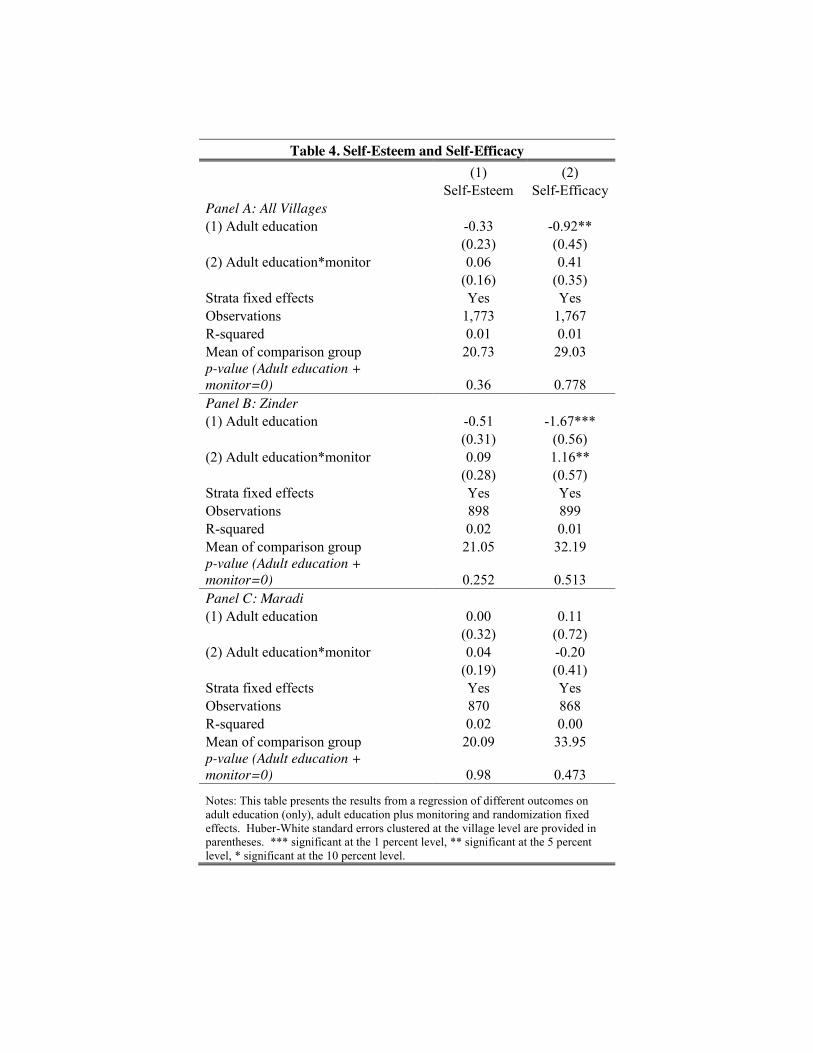
Table 4. Self-Esteem and Self-Efficacy

(1) (2)

Self-Esteem Self-Efficacy

Panel A: All Villages (1) Adult education -0.33 -0.92**

(0.23) (0.45)

(2) Adult education*monitor 0.06 0.41

(0.16) (0.35)

Strata fixed effects Yes Yes Observations 1,773 1,767 R-squared 0.01 0.01 Mean of comparison group 20.73 29.03 p-value (Adult education + monitor=0) 0.36 0.778 Panel B: Zinder

(1) Adult education -0.51 -1.67***

(0.31) (0.56)

(2) Adult education*monitor 0.09 1.16**

(0.28) (0.57)

Strata fixed effects Yes Yes Observations 898 899 R-squared 0.02 0.01 Mean of comparison group 21.05 32.19 p-value (Adult education + monitor=0) 0.252 0.513 Panel C: Maradi

(1) Adult education 0.00 0.11

(0.32) (0.72)

(2) Adult education*monitor 0.04 -0.20

(0.19) (0.41)

Strata fixed effects Yes Yes Observations 870 868 R-squared 0.02 0.00 Mean of comparison group 20.09 33.95 p-value (Adult education + monitor=0) 0.98 0.473

Notes: This table presents the results from a regression of different outcomes on adult education (only), adult education plus monitoring and randomization fixed effects. Huber-White standard errors clustered at the village level are provided in parentheses. *** significant at the 1 percent level, ** significant at the 5 percent level, * significant at the 10 percent level.

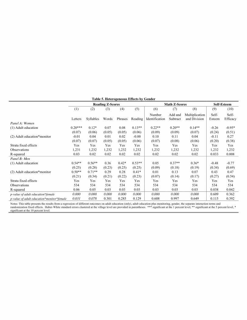
Table 5. Heterogeneous Effects by Gender

Reading Z-Scores Math Z-Scores Self-Esteem

(1) (2) (3) (4) (5) (6) (7) (8) (9) (10)

Letters Syllables Words Phrases Reading


Add and Subtract

Multiplication and Division

Self-Esteem

Self-Efficacy

Panel A: Women

(1) Adult education 0.20*** 0.12* 0.07 0.08 0.13** 0.22** 0.20** 0.14** -0.26 -0.95*

(0.07) (0.06) (0.05) (0.05) (0.06) (0.09) (0.09) (0.07) (0.24) (0.51)

(2) Adult education*monitor -0.01 0.04 0.01 0.02 -0.00 0.10 0.11 0.04 -0.11 0.27

(0.07) (0.07) (0.05) (0.05) (0.06) (0.07) (0.08) (0.06) (0.20) (0.38)

Strata fixed effects Yes Yes Yes Yes Yes Yes Yes Yes Yes Yes Observations 1,231 1,232 1,232 1,232 1,232 1,232 1,232 1,232 1,232 1,232 R-squared 0.03 0.02 0.02 0.02 0.02 0.02 0.02 0.02 0.033 0.008 Panel B: Men

(1) Adult education 0.54** 0.56** 0.36 0.42* 0.53** 0.05 0.37** 0.36* -0.48 -0.77

(0.25) (0.28) (0.23) (0.25) (0.25) (0.09) (0.18) (0.19) (0.34) (0.69)

(2) Adult education*monitor 0.50** 0.71** 0.29 0.28 0.41* 0.01 0.13 0.07 0.43 0.47

(0.21) (0.34) (0.21) (0.22) (0.23) (0.07) (0.14) (0.17) (0.27) (0.54)

Strata fixed effects Yes Yes Yes Yes Yes Yes Yes Yes Yes Yes Observations 534 534 534 534 534 534 534 534 534 534 R-squared 0.06 0.05 0.03 0.03 0.03 0.03 0.03 0.03 0.038 0.042 p-value of adult education*female 0.000 0.000 0.000 0.000 0.000 0.000 0.000 0.000 0.609 0.362 p-value of adult education*monitor*female 0.031 0.078 0.301 0.285 0.129 0.608 0.997 0.649 0.115 0.392 Notes: This table presents the results from a regression of different outcomes on adult education (only), adult education plus monitoring, gender, the separate interaction terms and randomization fixed effects. Huber-White standard errors clustered at the village level are provided in parentheses. *** significant at the 1 percent level, ** significant at the 5 percent level, * significant at the 10 percent level.

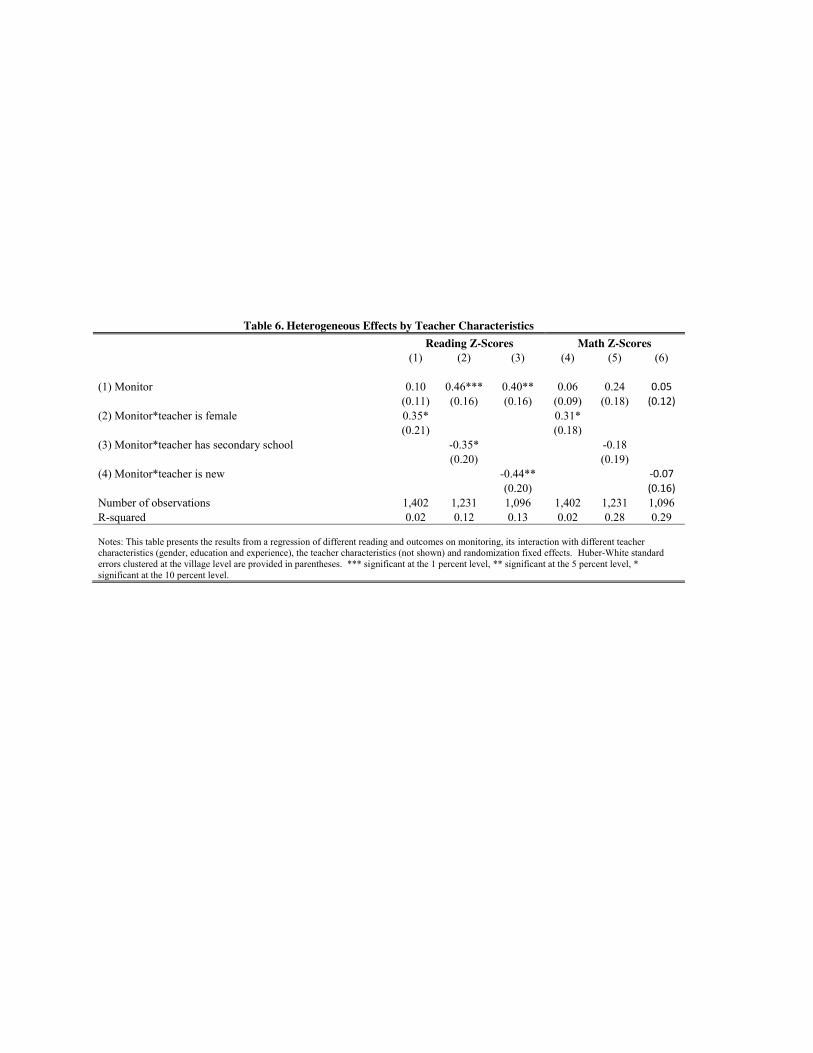
Table 6. Heterogeneous Effects by Teacher Characteristics

Reading Z-Scores Math Z-Scores

(1) (2) (3) (4) (5) (6)

(1) Monitor 0.10 0.46*** 0.40** 0.06 0.24 0.05

(0.11) (0.16) (0.16) (0.09) (0.18) (0.12)

(2) Monitor*teacher is female 0.35*

0.31*

(0.21)

(0.18)

(3) Monitor*teacher has secondary school

-0.35*

-0.18

(0.20)

(0.19)

(4) Monitor*teacher is new

-0.44**

-0.07

(0.20)

(0.16)

Number of observations 1,402 1,231 1,096 1,402 1,231 1,096 R-squared 0.02 0.12 0.13 0.02 0.28 0.29

Notes: This table presents the results from a regression of different reading and outcomes on monitoring, its interaction with different teacher characteristics (gender, education and experience), the teacher characteristics (not shown) and randomization fixed effects. Huber-White standard errors clustered at the village level are provided in parentheses. *** significant at the 1 percent level, ** significant at the 5 percent level, * significant at the 10 percent level.

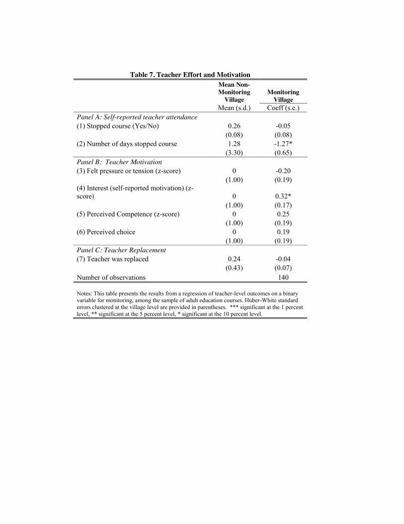
Table 7. Teacher Effort and Motivation

Mean Non-Monitoring

Village Monitoring

Village

Mean (s.d.) Coeff (s.e.)

Panel A: Self-reported teacher attendance (1) Stopped course (Yes/No) 0.26 -0.05

(0.08) (0.08)

(2) Number of days stopped course 1.28 -1.27* (3.30) (0.65) Panel B: Teacher Motivation

(3) Felt pressure or tension (z-score) 0 -0.20

(1.00) (0.19)

(4) Interest (self-reported motivation) (z-score) 0 0.32*

(1.00) (0.17)

(5) Perceived Competence (z-score) 0 0.25

(1.00) (0.19)

(6) Perceived choice 0 0.19

(1.00) (0.19)

Panel C: Teacher Replacement (7) Teacher was replaced 0.24 -0.04

(0.43) (0.07)

Number of observations 140

Notes: This table presents the results from a regression of teacher-level outcomes on a binary variable for monitoring, among the sample of adult education courses. Huber-White standard errors clustered at the village level are provided in parentheses. *** significant at the 1 percent level, ** significant at the 5 percent level, * significant at the 10 percent level.

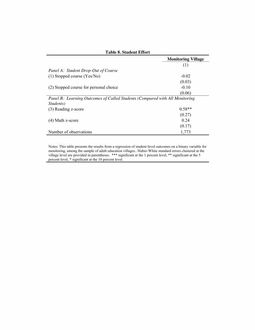
Table 8. Student Effort

Monitoring Village

(1)

Panel A: Student Drop-Out of Course (1) Stopped course (Yes/No) -0.02

(0.03)

(2) Stopped course for personal choice -0.10 (0.06) Panel B: Learning Outcomes of Called Students (Compared with All Monitoring Students) (3) Reading z-score 0.58**

(0.27)

(4) Math z-score 0.24

(0.17)

Number of observations 1,773

Notes: This table presents the results from a regression of student-level outcomes on a binary variable for monitoring, among the sample of adult education villages.. Huber-White standard errors clustered at the village level are provided in parentheses. *** significant at the 1 percent level, ** significant at the 5 percent level, * significant at the 10 percent level.

Table A1 Attrition

(1) (2) (3)

Comparison

Adult Education

Only

Adult Education + Monitoring

Panel A. Attrition Mean (s.d.) Coef (s.e.) Coef (s.e.) Attrition 0.05 0.041* -0.04** (0.22) (0.02) (0.01) Panel B. Characteristics of Non-Attriters

Female 0.69 0.03* -0.03

(0.46) (0.02) (0.02)

Age 31.83 1.80 0.19

(12.41) (1.45) (0.90)

Maradi 0.31 0.00 0.00

(0.46) (0.00) (0.00)

Notes: Panel A shows the results of a regression of a binary variable for attrition on adult education, monitoring and stratification fixed effects. Panel B shows the results of a regression of student characteristics among non-attriters on adult education, monitoring and stratification fixed effects. Huber-White standard errors clustered at the village level are provided in parentheses. *** significant at the 1 percent level, ** significant at the 5 percent level, * significant at the 10 percent level.

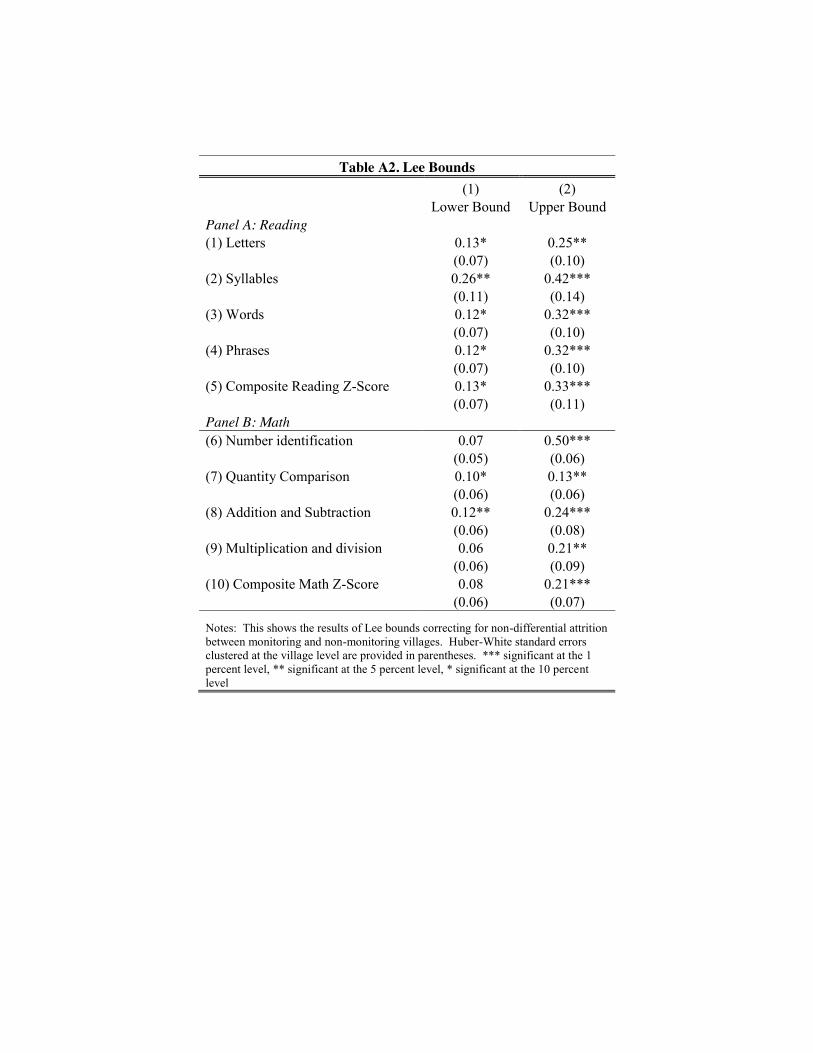
Table A2. Lee Bounds

(1) (2)

Lower Bound Upper Bound

Panel A: Reading (1) Letters 0.13* 0.25**

(0.07) (0.10)

(2) Syllables 0.26** 0.42***

(0.11) (0.14)

(3) Words 0.12* 0.32***

(0.07) (0.10)

(4) Phrases 0.12* 0.32***

(0.07) (0.10)

(5) Composite Reading Z-Score 0.13* 0.33***

(0.07) (0.11)

Panel B: Math (6) Number identification 0.07 0.50***

(0.05) (0.06)

(7) Quantity Comparison 0.10* 0.13**

(0.06) (0.06)

(8) Addition and Subtraction 0.12** 0.24***

(0.06) (0.08)

(9) Multiplication and division 0.06 0.21**

(0.06) (0.09)

(10) Composite Math Z-Score 0.08 0.21***

(0.06) (0.07)

Notes: This shows the results of Lee bounds correcting for non-differential attrition between monitoring and non-monitoring villages. Huber-White standard errors clustered at the village level are provided in parentheses. *** significant at the 1 percent level, ** significant at the 5 percent level, * significant at the 10 percent level

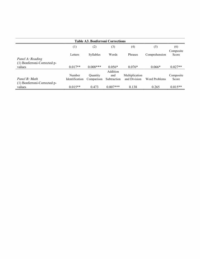
Table A3. Bonferroni Corrections

(1) (2) (3) (4) (5) (6)

Letters Syllables Words Phrases Comprehension

Composite Score

Panel A: Reading (1) Bonferroni-Corrected p-

values 0.017** 0.008*** 0.056* 0.076* 0.066* 0.027**

Panel B: Math Number

Identification Quantity

Comparison

Addition and

Subtraction Multiplication and Division Word Problems

Composite Score

(1) Bonferroni-Corrected p-values 0.015** 0.473 0.007*** 0.138 0.265 0.015**

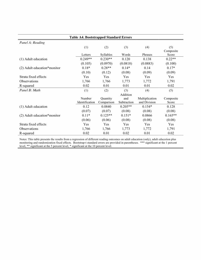
Table A4. Bootstrapped Standard Errors Panel A: Reading

(1) (2) (3) (4) (5)

Letters Syllables Words Phrases

Composite Score

(1) Adult education 0.249** 0.230** 0.120 0.138 0.22**

(0.105) (0.0970) (0.0818) (0.0883) (0.100)

(2) Adult education*monitor 0.18* 0.28** 0.14* 0.14 0.17*

(0.10) (0.12) (0.08) (0.09) (0.09)

Strata fixed effects Yes Yes Yes Yes Yes Observations 1,766 1,766 1,773 1,772 1,791 R-squared 0.02 0.01 0.01 0.01 0.02 Panel B: Math (1) (2) (3) (4) (5)


Quantity Comparison

Addition and

Subtraction Multiplication and Division

Composite Score

(1) Adult education 0.12 0.0840 0.205** 0.154* 0.128

(0.07) (0.07) (0.08) (0.08) (0.08)

(2) Adult education*monitor 0.11* 0.125** 0.151* 0.0866 0.165**

(0.06) (0.06) (0.08) (0.08) (0.08)

Strata fixed effects Yes Yes Yes Yes Yes Observations 1,766 1,766 1,773 1,772 1,791 R-squared 0.02 0.01 0.02 0.01 0.02

Notes: This table presents the results from a regression of different reading outcomes on adult education (only), adult education plus monitoring and randomization fixed effects. Bootstrap-t standard errors are provided in parentheses. *** significant at the 1 percent level, ** significant at the 5 percent level, * significant at the 10 percent level.

Table A5. Excluding Called Students

Panel A: Reading

(1) (2) (3) (4) (5)

Letters Syllables Words Phrases Composite Score

(1) Adult education 0.27*** 0.22** 0.13 0.14* 0.23**

-0.1 (0.10) (0.08) (0.09) (0.10)

(2) Adult education*monitor 0.16* 0.26** 0.11 0.10 0.16*

-0.09 (0.13) (0.08) (0.08) (0.09)

Strata fixed effects Yes -0.23 Yes Yes Yes Observations 1,732 1,732 1,732 1,732 1,732 R-squared 0.02 0.01 0.01 0.01 0.02 Panel B: Math (1) (2) (3) (4) (5)


Quantity Comparison

Addition and Subtraction

Multiplication and Division Composite Score

(1) Adult education 0.12* 0.08 0.21** 0.17* 0.13

(0.07) (0.07) -0.09 (0.09) (0.08)

(2) Adult education*monitor 0.10* 0.13** 0.14* 0.07 0.16**

(0.06) (0.06) -0.08 (0.08) (0.07)

Strata fixed effects Yes Yes Yes Yes Yes Observations 1,732 1,732 1,732 1,732 1,732 R-squared 0.02 0.01 0.02 0.01 0.02

Notes: This table presents the results from a regression of different reading outcomes on adult education (only), adult education plus monitoring and randomization fixed effects. Huber-White standard errors clustered at the village level are provided in parentheses. *** significant at the 1 percent level, ** significant at the 5 percent level, * significant at the 10 percent level.

Figure 1. Map of Intervention Areas

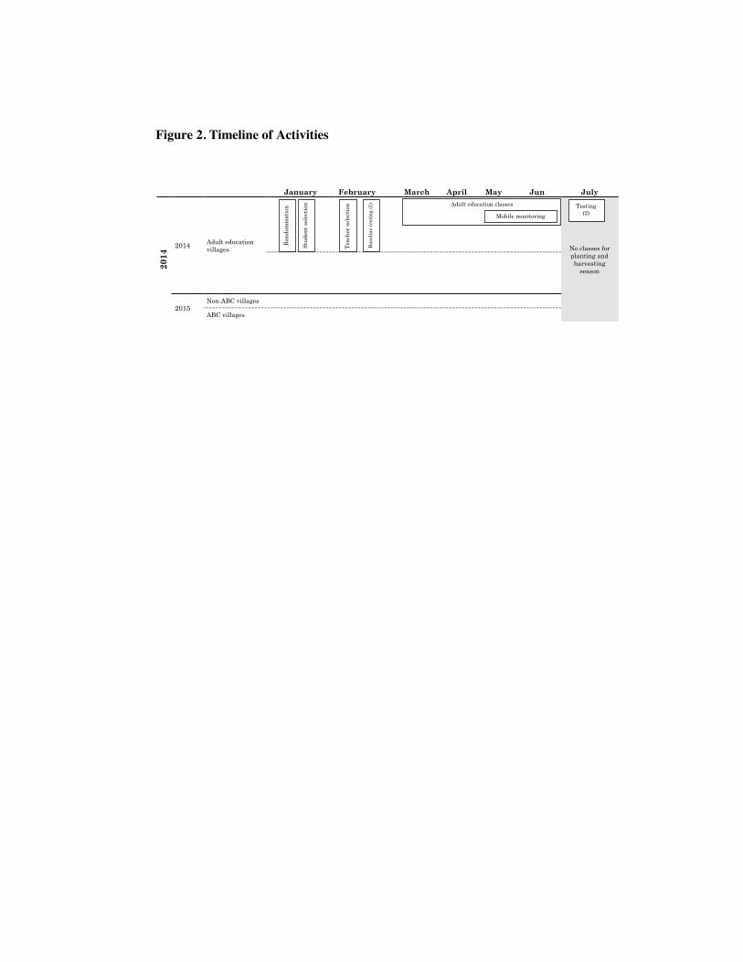
Figure 2. Timeline of Activities

January February March April May Jun July

2014

2014 Adult education villages

No classes for planting and harvesting

season

2015 Non-ABC villages

ABC villages

Ran

dom

izat

ion

Stud

ent

sele

ctio

n

Bas

elin

e te

stin

g (1

) Adult education classes Testing (2) Mobile monitoring

Tea

cher

sel

ecti

on

and

trai

ning

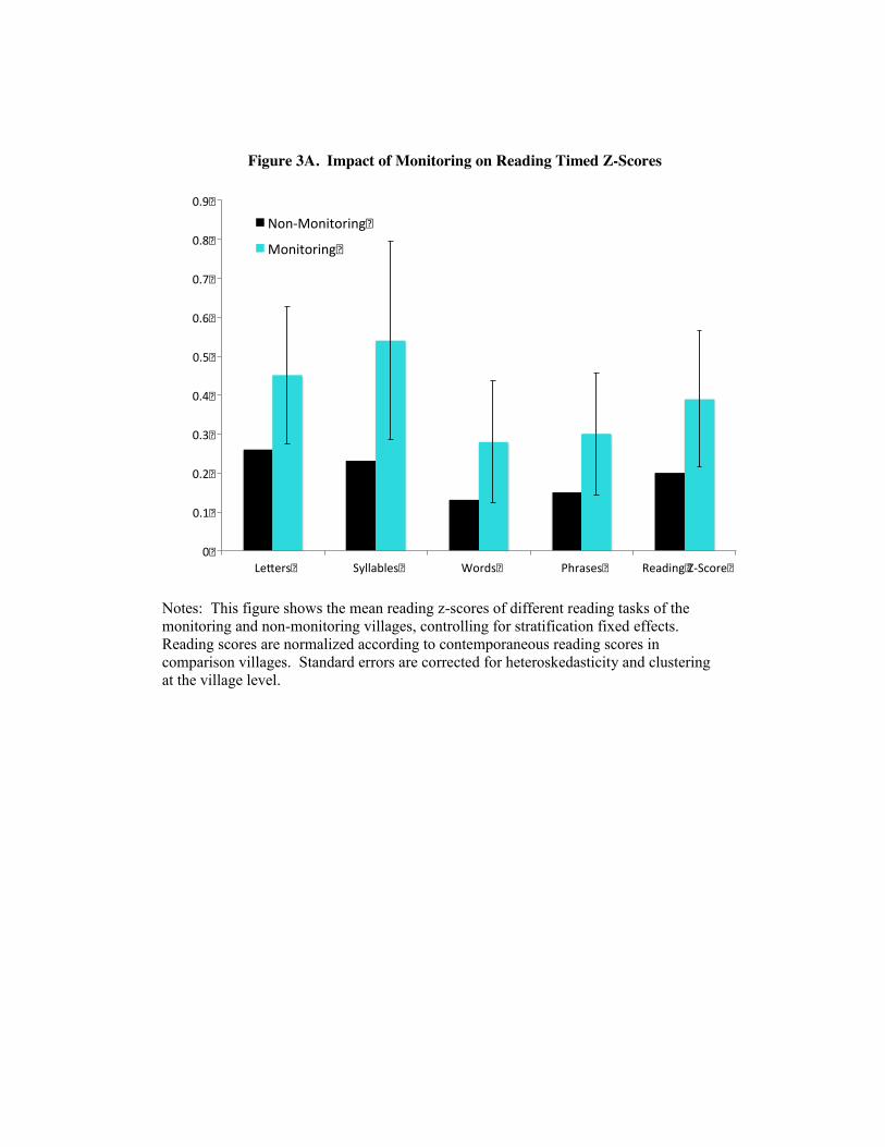
Figure 3A. Impact of Monitoring on Reading Timed Z-Scores

Notes: This figure shows the mean reading z-scores of different reading tasks of the monitoring and non-monitoring villages, controlling for stratification fixed effects. Reading scores are normalized according to contemporaneous reading scores in comparison villages. Standard errors are corrected for heteroskedasticity and clustering at the village level.

0�

0.1�

0.2�

0.3�

0.4�

0.5�

0.6�

0.7�

0.8�

0.9�

Le ers� Syllables� Words� Phrases� Reading�Z-Score�

Non-Monitoring�

Monitoring�

Figure 3B. Impact of Monitoring on Math Z-Scores

Notes: This figure shows the mean math z-scores of different math tasks of the monitoring and non-monitoring villages, controlling for stratification fixed effects. Math scores are normalized according to contemporaneous math scores in comparison villages. Standard errors are corrected for heteroskedasticity and clustering at the village level.

0�

0.1�

0.2�

0.3�

0.4�

0.5�

0.6�

#�Iden fica on� #�Iden fica on�2� Add/Subtract� Mul ply/Divide� Math�Z-Score�

Non-Monitoring�

Monitoring�

Documents

Call Me Educated 27aug2015 - sites.tufts.edu · In rural areas of developing countries, public worker absence – of teachers, doctors, nurses or agricultural extension agents –