Embed Size (px)
Citation preview

1
CALYPSO: a method for crystal structure prediction
Yanchao Wang, Jian Lv, Li Zhu and Yanming Ma*
State Key Laboratory of Superhard Materials, Jilin University, Changchun 130012,
China
We have developed a software package CALYPSO (Crystal structure AnaLYsis by
Particle Swarm Optimization) to predict the energetically stable/metastable crystal
structures of materials at given chemical compositions and external conditions (e.g.,
pressure). The CALYPSO method is based on several major techniques (e.g.
particle-swarm optimization algorithm, symmetry constraints on structural generation,
bond characterization matrix on elimination of similar structures, partial random
structures per generation on enhancing structural diversity, and penalty function, etc)
for global structural minimization from scratch. All of these techniques have been
demonstrated to be critical to the prediction of global stable structure. We have
implemented these techniques into the CALYPSO code. Testing of the code on many
known and unknown systems shows high efficiency and high successful rate of this
CALYPSO method [Wang et al., Phys. Rev. B 82 (2010) 094116][1]. In this paper, we
focus on descriptions of the implementation of CALYPSO code and why it works.

2
1. Introduction
Understanding the behaviors of materials at the atomic scale is fundamental to
modern science and technology. As many properties and phenomena are ultimately
controlled by the crystal structures, the prediction of crystal structure is an important
task in chemistry and condensed matter physics. However, the structural prediction
with the only known information of chemical compositions is extremely difficult as it
basically involves in classifying a huge number of energy minima on the lattice
energy surface. Owing to the significant progress in both computational power and
basic materials theory, it is now possible to predict the crystal structure at zero Kelvin
using the quantum mechanical methods. One way to predict structure is by extracting
known structures from databases of structures previously found in similar materials[2].
However, this method has a limited success rate and is incapable of generating new
crystal structure types. Recently, the more advanced methods including simulated
annealing[3, 4], minima hopping[5], basin hopping[6], metadynamics[7], genetic
algorithm[8-15], and random sampling method[16]have been developed and applied,
which allow a systematic search for the ground state structures based on the chemical
composition and the external conditions. The simulated annealing, basin hopping,
minima hopping and metadynamics focus on overcoming the energy barriers and are
successful in many researches[3-7], particularly, when the starting structure is close to
the global minimum. The genetic algorithm starts to use a self-improving method and
is thus able to correctly predict many structures [17-20]. The random sampling
method, as a simple and efficient method, is also successful in many applications
[21-24].
The particle swarm optimization(PSO), first proposed by Kennedy and Eberhart
[25, 26], is a population-based optimization method. As a stochastic global
optimization method, PSO is inspired by the choreography of a bird flock and can be
seen as a distributed behavior algorithm that performs multidimensional search.
According to PSO, the behavior of each individual is affected by either the best local
or the best global individual to help it fly through a hyperspace. Moreover, an
individual can learn from its past experiences to adjust its flying speed and direction.
3
Therefore, all the individuals in the swarm can quickly converge to the global position.
PSO algorithm is a highly efficient global optimization method which has been
applied successfully into many optimization problems such as network training [27,
28] and transactions on power systems[29]. However, the application of PSO to the
structural prediction of condensed matters remains a major challenge. Due to the
existence of a large number of energy minima on the lattice energy surface, rapid
swarm convergence, as one of the main advantages of PSO, can also be problematic.
If an early solution is sub-optimal, the swarm can easily stagnate around it without
any pressure to continue further exploration, i.e., the premature. We recently have
developed a CALYPSO method/code[1] on crystal structure prediction by
implementation of PSO algorithm and many other important techniques, including
symmetry constraints on structural generation, bond characterization matrix on
elimination of similar structures, partial random structures per generation on
enhancing structural diversity, and penalty function, etc. We found that these later
techniques are critical to avoid the premature of PSO algorithm and to significantly
accelerate the structure convergence.
The description of CALYPSO method and its first applications to the prediction
of crystal structures can be found in Ref.[1]. This paper is organized as follows. The
detailed descriptions of implementation of CALYPSO code and the principles on
illustrating why the method works are presented in Section 2. In Section 3, various
parameters in CALYPSO code are optimized for TiO2 as a benchmark. The input and
output files are provided in Sections 4. A short overview of the applications obtained
from our method can be found in Section 5, followed by the conclusion in Section 6.
2. Implementation and discussions
As depicted in the pseudo-code of Algorithm1, the CALYPSO method comprises
mainly four steps: (i) generation of random structures with the constraint of symmetry;
(ii) local structural optimization; (iii) post-processing for the identification of unique
local minima by bond characterization matrix; (iv) generation of new structures by
PSO for iterations.
2.1 Symmetry constraints on structural generation

4
There are two types of variables to define a crystal structure: lattice parameters
(three angles and the lengths of the three lattice vectors) and atomic coordinates (three
coordinates coded as a fraction of the lattice vector for each atom). The first step of
CALYPSO method is to generate random structures constrained within 230 space
groups. Once a particular space group is selected, the lattice parameters are generated
within the chosen symmetry according to the confined volume and the corresponding
atomic coordinates are obtained by a combination of a set of symmetrically related
coordinates (Wyckoff Positions) in accordance to the number of atoms in the
simulation cell. For example, if the confined volume is 64 Å3 and there are 12 atoms
in the simulation cell for the group 223(Pm-3n), the lengths of three lattice vectors
should be 4 Å and the lattice angles are fixed to 90, while the atomic positions can be
combined by different Wyckoff Positions (e.g., 6b + 6c, 6b + 6d, and 12f, etc).
Moreover, a list including the symmetric information (space group) of all generated
structures is built and used to compare with the newly generated structures. The
appearance of identical symmetric structures is forbidden with a certain probability
(80%). This makes the initial sampling covered different regions of the search space,
which is crucial for the diversity of population. The generation of random structures
ensures unbiased sampling of the energy landscape. The explicit application of
symmetric constraints leads to significantly reduced search space and optimization
variables, and thus fastens global structural convergence.
In order to examine the efficiency of symmetric constraints as implemented in
CALYPSO code, the system of TiO2with 16 TiO2 units (48 atoms) per simulation cell
was used as a test case. 3250 structures at ambient pressure were randomly generated
and then structurally optimized using the GULP code[30] with a combination of
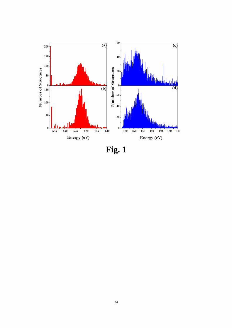
Buckingham and Lennard-Jones potentials[11, 31]. Fig. 1 (a) and (b) show the energy
distributions of these generated structures with and without symmetry constraints,
respectively. It is found that the rutile structure, i.e., the global stable structure cannot
be generated if without symmetry constraints. However, once the symmetry is
implemented in the generation of random structures, 203 (~6.2% in total) rutile
structures were successfully produced. In order to further compare the structural

5
search efficiency of generation of random structures with or without the symmetry
constraints, the binary Lennard-Jones crystal A2B (18 atoms per simulation cell) was
used as another test case. 5000 structures were randomly generated and then
structurally optimized using the GULP code[30] with Lennard-Jones potentials
(AA=AA=1.0, BB=0.88, BB=0.5, AB=0.932 and AB=1.5)[32]. The energy
distributions of the structures generated with and without symmetry constraints are
shown in Fig. 1 (c) and (d), respectively. It is obvious that the energies of these
structures generated with symmetry constraints distribute lower energy regions. We
also have examined the structural search efficiency of CALYPSO runs with or without
the symmetry constraints on structural generation as shown in Table 1. Obviously, the
application of symmetry constraints technique can greatly improve the search
efficiency, especially for larger systems. It is found that an averaged 11 generations
are necessary to find the global stable structure if with the symmetry constraints on
structural generation, however if without, 25.4 generations are needed. These tests
clearly illustrate the importance of the symmetry constraints in the generation of
random structures for structure prediction.
2.2 Structural optimization
CALYPSO code currently can use ab initio packages (e.g., VASP[33, 34],
SIESTA[35] and CASTEP[36, 37]) and force-field program (e.g., GULP[30])to
perform the structural optimization. Other external programs can also be interfaced on
user’s request. The use of locally structural optimization techniques (e.g., line
minimization, steepest descents, conjugate gradient algorithm or
Broyden-Fletcher-Goldfarb-Shanno algorithm) leads the lattice energy to the local
minimum. Here, we use free energy (at T = 0 K, free energy reduces to enthalpy) as
fitness function throughout the simulation. Note that local optimization increases the
cost of each individual, but reduces effectively the noise of the energy landscape,
enhances comparability between different structures, and provides locally optimal
structures for further use. Thus, local optimization is crucial for the structure
prediction.
2.3 Elimination of similar structures by using the bond characterization

6
matrix
Our goal is to eliminate the similar structures in the structure generations to
enhance the search efficiency of CALYSPO. In our earlier implementation [1], we
used geometrical structure parameter, which is solely based on the bond length, to
identify structural similarity. Here, we have developed a more efficient technique
named as bond characterization matrix, which is on the basis of all the bond
information. In this method, we employ a set of modified bond-orientational order
metrics(Ql) introduced by Steinhardtet al[38] to quantify the bond angles and an
exponential function to quantify the bond length. When the distance between two
atoms is less than the cutoff (rcut), bond information, e.g. bond vector (ijr ), bond
angles ( ijij , ) and bond-types (AB), are evaluated, where ijr is a vector pointing
from ithatom to jthatom, while
ij ,ij are the related polar and azimuthal angles of
ijr , respectively, and A(B)is the type of ith(jth) atom. In this work, bond
characterization matrix is calculated according to the “bond-types”, where each vector
ijr can be represented by spherical harmonics ),( ijijlmY . Subsequently, for each
bond typeAB, a weighted average is performed,
AB ij AB
AB
δ -α(r -b )
lm ij ijlm
i A,j Bδ
1= Y θ ,
NeQ
(1)
whereAB
N is the number of bonds formed by type A and B atoms, bAB is the shortest
length for each bond type and is an adjusted parameter drivingeABcut br )( 0.In
order to avoid the dependence on the choice of reference frame, the averageAB
lmQ
is
used to calculate the rotationally invariant combinations,
24
2 1
ABAB
l
l lm
m l
Q Ql
(2)
Only even-l spherical harmonics, which are invariant with respect to the direction of
the bonds, are used in Eq. (2), and each structure can be characterized by bond
characterization matrix. The similarity between two structures is thus given by the

7
Euclidean distance of their bond characterization matrix.
1/ 22, ,
( )AB AB
AB
u vD Q Q
uv l ll
(3)
where u and v are individual structures.
As an illustrative case, the histograms of Ql versus l for graphite and diamond are
shown in Fig. 2 (a) and (b), respectively. Significant differences for Ql between these
two structures are evidenced, which illustrate the efficiency of the bond
characterization matrix method to distinguish different structures. To further
demonstrate the robust of the method, the Euclidean distances between
graphite/diamond and its random distortions are calculated as shown in Fig. 2
(c)/(d).It is clearly seen that the calculated Euclidean distances monotonously increase
with the magnitude of distortions. These tests highlight the capability of this bond
characterization matrix method in the characterization of the structural similarities.
We have implemented this bond characterization matrix technique into
CALYPSO code to eliminate similar structures. Table 2 shows the influence of this
technique on the search efficiency of CALYPSO calculations for the system of TiO2.
It is clearly seen that much fewer optimization steps are needed to find the stable
structure when this technique is included in the CALYPSO runs. This is
understandable since the use of bond characterization matrix technique can effectively
avoid the presence of very similar or identical structures and thus is able to accelerate
the global structure convergence.
2.4 Generation of new structures by PSO
Within the PSO scheme, a structure (an individual) in the searching space is
regarded as a particle. A set of individual structures is called a population. The lattice
parameters (unit cell) of new structures are the same as the corresponding structures
of the previous generation. While the atomic positions are updated using the
evolutionary equation (4). Note that all the new structures produced by PSO (or
randomly generated) are tested against constraint of minimal inter-atomic
distances[10].
8
1 1
, , ,
t t t
i j i j i jx x v (4)
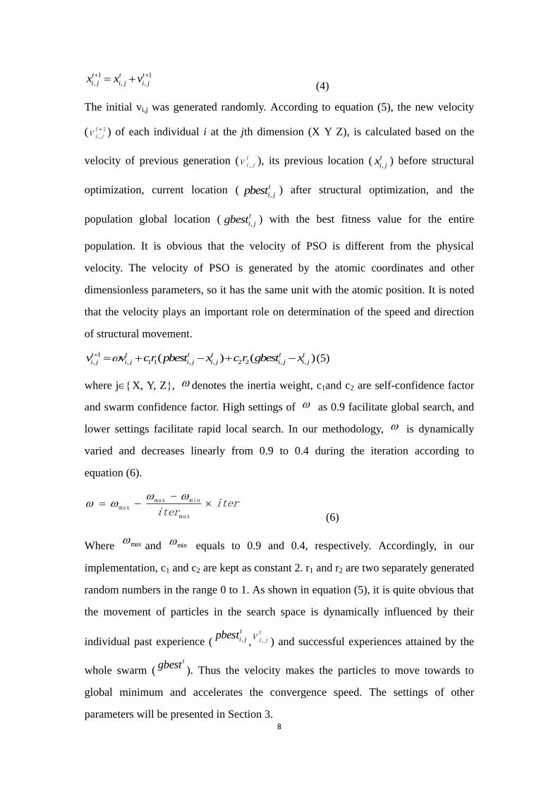
The initial vi,j was generated randomly. According to equation (5), the new velocity
( 1,tjiv ) of each individual i at the jth dimension (X Y Z), is calculated based on the
velocity of previous generation ( tjiv , ), its previous location (
,
t
i jx ) before structural
optimization, current location (,
t
i jpbest ) after structural optimization, and the
population global location (,
t
i jgbest ) with the best fitness value for the entire
population. It is obvious that the velocity of PSO is different from the physical
velocity. The velocity of PSO is generated by the atomic coordinates and other
dimensionless parameters, so it has the same unit with the atomic position. It is noted
that the velocity plays an important role on determination of the speed and direction
of structural movement.
1
, , 1 1 , , 2 2 , ,( ) ( )t t t t t t
i j i j i j i j i j i jv v cr pbest x c r gbest x (5)
where jX, Y, Z, denotes the inertia weight, c1and c2 are self-confidence factor
and swarm confidence factor. High settings of as 0.9 facilitate global search, and
lower settings facilitate rapid local search. In our methodology, is dynamically
varied and decreases linearly from 0.9 to 0.4 during the iteration according to
equation (6).
iteriter
max
minmaxmax
(6)
Where maxand min equals to 0.9 and 0.4, respectively. Accordingly, in our
implementation, c1 and c2 are kept as constant 2. r1 and r2 are two separately generated
random numbers in the range 0 to 1. As shown in equation (5), it is quite obvious that
the movement of particles in the search space is dynamically influenced by their
individual past experience (t
jipbest , ,tjiv , ) and successful experiences attained by the
whole swarm (tgbest). Thus the velocity makes the particles to move towards to
global minimum and accelerates the convergence speed. The settings of other
parameters will be presented in Section 3.

9
2.5 Penalty function
According to Bell-Evans-Polanyi principle[16, 39], the low energy basins in
potential energy surfaces are expected to occur near other low energy basins. Thus, in
order to improve the efficiency of the procedure, a certain number of high-energy
structures are rejected, and the remaining low energy structures, which are on the
most promising areas of the configuration space, are selected to produce the next
generation by PSO. Fig. 3 (a) and (b) show the evolution of lattice energy
distributions with and without the inclusion of penalty function during the simulation
(shown here for TiO2 with 48 atoms in the simulation cell). Obviously, most of
structures are in low-energy region (<620.0eV) when the penalty function technique is
included and it significantly accelerates the structural converges to the global
minimum as demonstrated in the CALYPSO runs (Fig. 3).
2.6 Structural diversity
Structural diversity plays an important role in the prediction of crystal structures
by using the population-based methods, such as the genetic algorithm and our
developed CALYPSO method. During the structural evolution, if the systems lose the
structural diversity, it is quite often that the systems stagnate, particularly for a large
system. We here have designed a critical technique to enhance the structural diversity
by including certain percentage of random structures in each generation, which has
been implemented in CALYPSO code. Again, we use TiO2 with 16 formula units per
simulation cell as a test example. The history of CALYPSO runs with and without
including the randomly generated structures is shown in Fig. 4. It is seen that the
inclusion of a certain number of structures whose symmetries must be distinguished
from any of previously generated ones is indeed crucial to converge the system to the
global minimum. This all comes to the true fact that the inclusion of random
structures allows the generation of diverse structures [Table 3]. Note that it might
come up with the question on if the global stable structure is in fact generated by
those random structures. We have performed a certain number of tests and found out
that only a few stable structures are generated randomly, especially for smaller
systems. For most of cases, the structural evolution of CALYPSO runs derives the
10
global stable structures.
2.7Convergence
The CALYPSO simulation is stopped when the halting criterion is reached. In
accordance with our experience, the stable crystal structure can usually be found at
~10 generations for systems 10 atoms per simulation cell. In practice, the halting
criterion in CALYPSO is by default set to10 further generations if the simulation can
not find other better structures.
3. Optimization of parameters
In order to provide reasonable default setting for various parameters in our
CALYPSO code, a test was performed on TiO2 system with 16 formula units per
simulation cell by using the GULP code for the structural optimization and total
energy calculations. Earlier study [26] has demonstrated that c1= c2= 2 and the linear
decrease of from 0.9 to 0.4 during the iteration usually give the best overall
performance for PSO simulations. Thus, we adopt these parameters and other
parameters such as the population size (NPOP), the proportion of the structures
generated by PSO(PPSO) and the max magnitudes of the velocity (Vmax) are
determined by using the benchmark of TiO2. We repeat 5 successful CALYPSO
calculations, i.e., the correct finding of rutile structure, to derive the proper parameters.
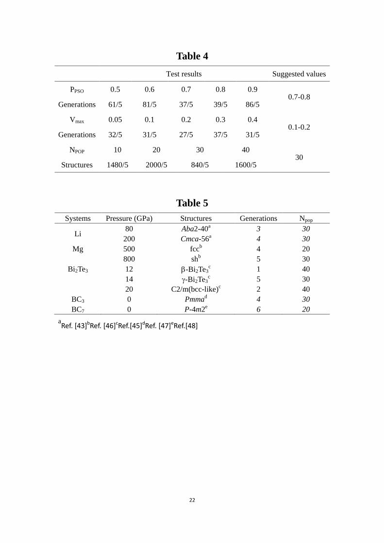
The results and suggested parameter values can be found in Table 4.
4. Input and output files
4.1 input file
The main input file named as input.dat, contains all the necessary parameters for
the simulation. There are several examples for the input.dat file in the Examples
directory of CALYPSO package.
We here take SiC as an example:
SystemName = SiC
NumberOfSpecies = 2
NameOfAtoms = C Si
NumberOfAtoms = 1 1
NumberOfFormula = 2 2

11
AtomicNumber = 6 14
MaxStep = 50
Volume= 20.0
@DistanceOfIon
1.2 1.5
1.5 1.9
@End
PsoRatio = 0.6
Icode= 1
Kgrid = 0.12 0.08
Command = vasp
PopSize = 20
PickUp = F
PickStep = 0
Here follows a description of the variables defined in the input file (input.dat),
including the data types and default values.
SystemName (string): A string of one or several words contains a descriptive
name of the system (max. 40 characters).
Defualt value: CALYPSO
NumberOfSpecies (integer): Number of different atomic species.
Default value: No default.
NameOfAtoms (string): Element symbols of the different chemical species.
Default value: No default.
AtomicNumber (integer): Atomic Number of each chemical species.
Default value: No default.
NumberOfAtoms (integer): Number of atoms for each chemical species in one
formula unit.
Default value: No default.
NumberOfFormula (integer): The desired range of formula units per simulation
cell. The first and second numbers are the lower and upper limits per simulation cell

12
in the formula units.
Default value: 1 4
Volume (real): The volume per formula unit. Unit is in Å3. The volume can be
estimated by the atomic volume of given elements. If it is set to zero, the program will
automatically generate the estimated volume by the radius of ions.
Default value: 0
@DistanceOfIon and @End (real): Minimal distances between different
chemical species. Unit is in angstrom. The determination of this parameter is in
accordance with “ NumberOfSpecies”. For example, if the NumberOfSpecies=2, a
22 matrix is used to indicate the minimal distances between different chemical
species.
@DistanceOfIon
d11 d12
d21 d22
@End
Default value: 0.7 Å
Icode(integer): It determines which local optimization package should be
interfaced with in the simulation.
1: VASP
2: SIESTA
3: GULP
4: CASTEP
Default value: 1
PsoRatio (real): The proportion of the structures generated by PSO, and the other
structures will be generated randomly.
Default value: 0.6
PopSize (integer): The population size. Normally, it will have a larger value for
larger systems.
Default value: 30
Kgrid (real): The precision of the K-point sampling for local optimization (VASP

13
or SIESTA). The Brillouin zone sampling uses a grid of spacing 2π×Kgrid Å-1. The
first value controls the precision of the first two local optimizations, and the second
value with denser K-points controls the last optimization. The smaller value normally
gives finer optimization results.
Default value: 0.12 0.06
Command (string): The command to perform local optimization on your
computer.
Default value: submit.sh.
MaxStep (integer): The maximum number of PSO iterations. It should have a
larger value for a larger system.
Default value: 50
PickUp(logical): If True, a previous calculation will be continued.
Default value: false
PickStep(integer): At which step will the previous calculation be picked up.
Default value: There is no default. If PickUp=True, you must supply this
variable.
4.2 output files
The main outputs of CALYPSO are in the “results” folder:
CALYPSO.log: It includes the information of the structures (the space group, the
volume, the number of atoms, et al.).
similar.dat: It includes the bond characterization matrixes of predicted structures.
pso_ini_*: It includes the information of the initial structures of the *-th iteration
step.
pso_opt_*: It includes the enthalpy and structural information after local
optimization of the *-th iteration.
pso_sor_*: The enthalpy sorted in ascending order of the *-th iteration step.
5. Applications.
We have earlier illustrated that the CALYPSO method can be used to predict
various structures on elemental, binary and ternary compounds with various chemical
bonding environments (e.g., metallic, ionic, and covalent bonding)[1, 40, 41]. Here,

14
we discuss some other applications on the discovery of hitherto unknown structures.
All the ab initio structure relaxations were performed using density functional theory
within the projector augmented wave method, as implemented in the VASP code [33,
34]. An overview of systems with unknown structures for which we have performed
calculations and discovered new structures can be found in Table 5.
Lithium (Li) is a “simple” metal at ambient pressure, but exhibits complex phase
transitions under compression. Experimentally, it has been demonstrated that Li takes
the phase transition sequence of bcc→ fcc→ hR1 → cI16, above which new phases
are observed but remain unsolved[42]. We thus have extensively explored the
high-pressure phases of Li through CALYPSO code. We successfully predicted all the
experimental structures at certain pressure ranges by the CALYPSO method[1]. In
particular, two new orthorhombic Aba2-40 (40 atoms/cell) and Cmca-56(56
atoms/cell) structures of Li [43] were predicted at 80 and 200 GPa. These two
complex structures (Aba2-40 and Cmca-56) are successfully predicted only at the
third and fourth generation with a population size N pop of 30, respectively. Note that
Aba2-40 (oC40) structure has been later verified by an independent experiment[44].
Being a known best thermoelectric material and a topological insulator at
ambient condition, bismuth telluride experiences phase transitions into several
superconducting states under pressure. However, the high-pressure structures remain
unsolved since 1972. We have recently predicted two low-pressure phases of bismuth
telluride through CALYPSO calculations as seven-fold (-Bi2Te3) and eight-fold
(-Bi2Te3) monoclinic structures at 12 and 14 GPa, respectively[45]. These two
structures were identified at the first and fifth generation with a population size of 30
and 40. These structures also have been subsequently verified by our experiment
through Reitveld refinement [45]. Other compounds (Mg[46], BC3[47]and BC7[48])
with unknown structures also are discovered at high pressure by CALYPSO
simulations [Table 5]. All the structures rapidly converge to the global minimum with
less than 150 local optimizations. These results demonstrated that our method is a
powerful and efficient tool on crystal structure determination.
The reason why our method is so successful can be traced to several powerful

15
techniques. Firstly, PSO is a highly efficient global optimization algorithm, which has
been applied successfully into many multi-objective optimization problems. Secondly,
symmetry constraints on structural generation make the initial sampling covered
different regions of the search space, which is crucial for the efficiency of global
minimization. Thirdly, the elimination of similar/identical structures using bond
characterization matrix technique and rejection of high-energy structures for each
generation are able to accelerate the global structural convergence. Fourth, the
inclusion of a certain number of structures whose symmetries are distinguished from
previous ones can keep the population diversity and is critical to the prediction of
global stable structures. Finally, the local optimization is effective reduce the noise of
the landscape and may also be one of the key issues for our method success.
6. Conclusions
In this paper, we outline descriptions of implementation of CALYPSO code,
which can be used to predict crystal structures of materials at given chemical
compositions and external conditions. Our CALYPSO method has incorporated
several major techniques (e.g. PSO algorithm, symmetry constraints on structural
generation, bond characterization matrix on elimination of similar structures, partial
random structures per generation on enhancing structural diversity, and penalty
function, etc), which have been demonstrated to be crucial to the prediction of global
stable structure. Suggested values for various parameters in CALYPSO have been
presented by performing benchmark on TiO2 system. The high success rate and high
efficiency on the structural searches of CALYPSO methodology have demonstrated
its reliability and promise as a major tool on crystal structure determination.
Program availability
CALYPSO is available via http://nlshm-lab.jlu.edu.cn/~calypso.html. The
software is free of charge for non-profit organizations, and delivered with the Fortran
source code. The details of installation instructions, the user’s manual in PDF format
and examples are included in the package.
Acknowledgement
The authors acknowledge the funding supports from the National Natural

16
Science Foundation of China under grant Nos. 11025418 and 91022029.
17
*Correspondence and requests for materials should be addressed to Y.M.
References
[1] Y. Wang, J. Lv, L. Zhu, Y. Ma, Phys. Rev. B, 82 (2010) 094116.
[2] J. Feng, W. Grochala, T. Jaronacute, R. Hoffmann, A. Bergara, N.W. Ashcroft, Phys. Rev. Lett., 96
(2006) 017006.
[3] S. Kirkpatrick, C.D. Gelatt, M.P. Vecchi, science, 220 (1983) 671.
[4] J. Pannetier, J. Bassas-Alsina, J. Rodriguez-Carvajal, V. Caignaert, Nature, 346 (1990) 343-345.
[5] M. Amsler, S. Goedecker, J. Chem. Phys. , 133 (2010) 224104.
[6] J. David, J.P.K. Doye, J. Phys. Chem. A, 101 (1997) 5111-5116.
[7] A. Laio, A. Rodriguez-Fortea, F.L. Gervasio, M. Ceccarelli, M. Parrinello, J. Phys. Chem. B, 109 (2005)
6714-6721.
[8] S.M. Woodley, P.D. Battle, J.D. Gale, C.R.A. Catlow, Phys. Chem. Chem. Phys., 6 (2004) 1815-1822.
[9] N. Abraham, M. Probert, Phys. Rev. B, 73 (2006) 224104.
[10] C.W. Glass, A.R. Oganov, N. Hansen, Comput. Phys. Commun., 175 (2006) 713-720.
[11] D.C. Lonie, E. Zurek, Comput. Phys. Commun., 182 (2011) 372-387
[12] G. Trimarchi, A. Zunger, Phys. Rev. B, 75 (2007) 104113.
[13] Y. Yao, J.S. Tse, K. Tanaka, Phys. Rev. B, 77 (2008) 052103.
[14] D. Deaven, K. Ho, Phys. Rev. Lett., 75 (1995) 288-291.
[15] J.A. Niesse, H.R. Mayne, J. Chem. Phys. , 105 (1996) 4700.
[16] C.J. Pickard, R. Needs, J. Phys.: Condens. Matter 23 (2011) 053201.
[17] Y. Ma, M. Eremets, A.R. Oganov, Y. Xie, I. Trojan, S. Medvedev, A.O. Lyakhov, M. Valle, V.
Prakapenka, Nature, 458 (2009) 182-185.
[18] Y. Ma, A.R. Oganov, Z. Li, Y. Xie, J. Kotakoski, Phys. Rev. Lett. , 102 (2009) 65501.
[19] Y. Ma, Y. Wang, A.R. Oganov, Phys. Rev. B, 79 (2009) 054101.
[20] Q. Li, Y. Ma, A.R. Oganov, H. Wang, Y. Xu, T. Cui, H.K. Mao, G. Zou, Phys. Rev. Lett., 102 (2009)
175506.
[21] C.J. Pickard, R. Needs, Phys. Rev. Lett. , 97 (2006) 45504.
[22] C.J. Pickard, R. Needs, Nature Mater., 7 (2008) 775-779.
[23] C.J. Pickard, R. Needs, Phys. Rev. Lett. , 102 (2009) 146401.
[24] C.J. Pickard, R.J. Needs, Nature Phys., 3 (2007) 473-476.
[25] J. Kennedy, R.C. Eberhart, A discrete binary version of the particle swarm algorithm, (IEEE, 1997),
pp. 4104-4108 vol. 4105.
[26] R.C. Eberhart, Y. Shi, Particle swarm optimization: developments, applications and resources,
(Piscataway, NJ, USA: IEEE, 2001), pp. 81-86.
[27] R. Mendes, P. Cortez, M. Rocha, J. Neves, Particle swarms for feedforward neural network training,
in: Neural Networks, 2002. IJCNN '02. Proceedings of the 2002 International Joint Conference on (IEEE,
2002), pp. 1895-1899.
[28] M. Meissner, M. Schmuker, G. Schneider, BMC Bioinformatics, 7 (2006) 125.
[29] H. Yoshida, K. Kawata, Y. Fukuyama, S. Takayama, Y. Nakanishi, Power Systems, IEEE Transactions
on, 15 (2000) 1232-1239.
[30] J.D. Gale, J. Chem. Soc., Faraday Trans., 93 (1997) 629-637.
[31] S. Woodley, C. Catlow, Comput. Mater. Sci., 45 (2009) 84-95.

18
[32] J.R. Fernandez, P. Harrowell, J. Chem. Phys., 120 (2004) 9222.
[33] G. Kresse, J. Furthmuler, Comput. Mater. Sci., 6 (1996) 15-50.
[34] G. Kresse, J. Furthmuler, Phys. Rev. B, 54 (1996) 11169.
[35] J.M. Soler, E. Artacho, J.D. Gale, A. Garcia, J. Junquera, P. Ordejon, D. Sachez-Portal, J. Phys.:
Condens. Matter 14 (2002) 2745.
[36] S.J. Clark, M.D. Segall, C.J. Pickard, P.J. Hasnip, M.I.J. Probert, K. Refson, M.C. Payne, Z. Kristallogr. ,
220 (2005) 567-570.
[37] M. Segall, P.J.D. Lindan, M. Probert, C. Pickard, P. Hasnip, S. Clark, M. Payne, J. Phys.: Condens.
Matter 14 (2002) 2717.
[38] P.J. Steinhardt, D.R. Nelson, M. Ronchetti, Phys. Rev. B, 28 (1983) 784.
[39] F. Jensen, Introduction to computational chemistry, (Wiley, 2007).
[40] X. Luo, J. Yang, H. Liu, X. Wu, Y. Wang, Y. Ma, S.H. Wei, X. Gong, H. Xiang, J. Am. Chem. Soc. , 133
(2011) 16285–16290.
[41] H. Xiang, B. Huang, Z. Li, S. Wei, J. Yang, X. Gong, Phys. Rev. X, 2 (2012) 011003.
[42] T. Matsuoka, K. Shimizu, Nature, 458 (2009) 186-189.
[43] J. Lv, Y. Wang, L. Zhu, Y. Ma, Phys. Rev. Lett., 106 (2011) 15503.
[44] C.L. Guillaume, E. Gregoryanz, O. Degtyareva, M.I. McMahon, M. Hanfland, S. Evans, M. Guthrie,
S.V. Sinogeikin, H. Mao, Nature Phys., 7 (2011) 211–214.
[45] L. Zhu, H. Wang, Y. Wang, J. Lv, Y. Ma, Q. Cui, G. Zou, Phys. Rev. Lett. , 106 (2011) 145501.
[46] P. Li, G. Gao, Y. Wang, Y. Ma, J. Phys. Chem. C, 114 (2010) 21745–21749.
[47] H. Liu, Q. Li, L. Zhu, Y. Ma, Phys. Lett. A 375 (2011) 771-774.
[48] H. Liu, Q. Li, L. Zhu, Y. Ma, Solid State Commun. , 151 (2011) 716-719

19
Table and Figure captions
TABLE 1 The structural search efficiency of CALYPSO calculations with or without
the symmetric constraints on structural generation for the system of TiO2.We have
performed ten different CALYPSO runs and the total generations for these ten runs
needed to find the global stable rutile structure are listed. As an illustration, we choose
here the population size as 20. Notably, we generally use larger population sizes for
larger systems; there much less generations are needed to find the stable structure.
Other typical CALYPSO run parameters of Vmax and the percentage of PSO generated
structures are chosen as 0.1 and 0.6, respectively.
TABLE 2 The structural search efficiency of CALYPSO calculations with or without
the elimination of similar structures for the system of TiO2.We have performed ten
different CALYPSO runs and the total generations for these ten runs needed to find
the global stable rutile structure are listed. As an illustration, we choose here the
population size as 20. Notably, we generally use larger population sizes for larger
systems; there much less generations are needed to find the stable structure. Other
typical CALYPSO run parameters of Vmax and the percentage of PSO generated
structures are chosen as 0.1 and 0.6, respectively.
TABLE 3 The structural search efficiency of CALYPSO calculations with or without
partial random structures per generation for the system of TiO2.We have performed
ten different CALYPSO runs and the total generations for these ten runs needed to
find the global stable rutile structure are listed. As an illustration, we choose here the
population size as 20. Notably, we generally use larger population sizes for larger
systems; there much less generations are needed to find the stable structure. Other
typical CALYPSO run parameter of Vmax is chosen as 0.1.
TABLE 4 The test of variable parameters in CALYPSO.
TABLE 5 Systems with unknown structures, for which we have done calculations

20
and revealed new structures.
Algorithm 1. The pseudo-code of the implementation of CALYPSO.
FIG. 1. (color online) The energy distributions of randomly generated structures
containing 16 TiO2 units in the simulation cell and 6 units of binary Lennard-Jones
crystal A2B in the simulation cell after local optimization. (a) and (b) indicate the
energy distribution of TiO2 structures generated with and without the symmetric
constraints, respectively. (c) and (d) indicate the energy distribution of A2B structures
generated with and without the symmetric constraints, respectively.
FIG. 2. (color online)(a) and (b) Ql histograms for graphite and diamond structures,
respectively. (c) and (d) distance against distortion for graphite and diamond
structures, respectively. The unit of distortion magnitude is in bond length.
FIG. 3. (color online)(a) and (b) represent the evolution of lattice energy distributions
during structural iterations with and without the inclusion of penalty function,
respectively.
FIG. 4. (color online) The history of CALYPSO search performed on TiO2 with 48
atoms per cell. The red line represents the CALYPSO runs on that a certain number of
the low energy structures (0.6 of total) are selected to produce the next generation by
PSO, while the rest of structures are generated randomly. The green line represents
that all the structures are used to generate the next generation by PSO. Note that the
stable structure is produced by PSO in these calculations.

21
Table 1
Number of atoms in the system
12 24 36 48
Generations Generations Generations Generations
Symmetry constraints 12 15 85 110
No symmetry constraints 12 25 138 254
Table 2
Number of atoms in the system
12 24 36 48
Generations Generations Generations Generations
To eliminate similar
structures
11 14 21 78
To preserve similar
structures
10 17 47 118
Table 3
Number of atoms for TiO2
12 24 36 48
PPSO Generations Generations Generations Generations
0.6 12 15 85 110
1.0 11 23 124 229/9a
aIt fails to find the global stable structure in 100 generations one time out of ten.
22
Table 4
Test results Suggested values
PPSO 0.5 0.6 0.7 0.8 0.9 0.7-0.8
Generations 61/5 81/5 37/5 39/5 86/5
Vmax 0.05 0.1 0.2 0.3 0.4 0.1-0.2
Generations 32/5 31/5 27/5 37/5 31/5
NPOP 10
1480/5
20
2000/5
30
840/5
40
1600/5 30
Structures
Table 5
Systems Pressure (GPa) Structures Generations Npop
Li 80 Aba2-40
a 3 30
200 Cmca-56a 4 30
Mg 500 fccb 4 20
800 shb 5 30
Bi2Te3 12 -Bi2Te3c 1 40
14 -Bi2Te3c 5 30
20 C2/m(bcc-like)c 2 40
BC3 0 Pmmad 4 30
BC7 0 P-4m2e 6 20
aRef. [43]bRef. [46]cRef.[45]dRef. [47]eRef.[48]

23
Number of particles, N; swarm, S; volume, V; Percentage of PSO generated
structures, PPSO.
Initialization of S (Generation of random structures with constraint of symmetry)
Evaluation of S (Local optimization) and definition of the pbest and gbest
List of the bond characterization matrixes (BCM)
While not done do
SPSO=S*PPSO and Srandom=S*(1-PPSO)
While i<=SPSO do
S(i)(Generation of new structures by PSO)
If S(i) BCM then
i=i+1
To update the list of BCM
End if
End while
While i <=SPSO+Srandom
S(i) Generation of random structures with constraints of symmetry
If S(i) BCM then
i=i+1
To update the list of BCM
End if
End while
To Evaluate S (local optimization) and update the gbest
To update the list of BCM
End while
Algorithm 1
24
Fig. 1

25
Fig. 2

26
Fig. 3

27
Fig. 4