Embed Size (px)
Citation preview

This page intentionally left blank
CAMBRIDGE STUDIES IN ADVANCED MATHEMATICS 125
Editorial BoardB. BOLLOBÁS, W. FULTON, A. KATOK, F. KIRWAN,P. SARNAK, B. SIMON, B. TOTARO
p-adic Differential Equations
Over the last 50 years the theory of p-adic differential equations has grown into anactive area of research in its own right, and has important applications to numbertheory and to computer science. This book, the first comprehensive and unifiedintroduction to the subject, improves and simplifies existing results as well asincluding original material.
Based on a course given by the author at MIT, this modern treatment is accessible tograduate students and researchers. Exercises are included at the end of each chapter tohelp the reader review the material, and the author also provides detailed referencesto the literature to aid further study.
K I R A N S . K E D L AYA is Associate Professor of Mathematics at theMassachusetts Institute of Technology.

CAMBRIDGE STUDIES IN ADVANCED MATHEMATICSEditorial Board:
B. Bollobás, W. Fulton, A. Katok, F. Kirwan, P. Sarnak, B. Simon, B. Totaro
All the titles listed below can be obtained from good booksellers or from CambridgeUniversity Press. For a complete series listing visit:http://www.cambridge.org/series/sSeries.asp?code=CSAM
Already published
73 B. Bollobás Random graphs (2nd edition)74 R. M. Dudley Real analysis and probability (2nd edition)75 T. Sheil-Small Complex polynomials76 C. Voisin Hodge theory and complex algebraic geometry, I77 C. Voisin Hodge theory and complex algebraic geometry, II78 V. Paulsen Completely bounded maps and operator algebras79 F. Gesztesy & H. Holden Soliton equations and their algebro-geometric solutions, I81 S. Mukai An introduction to invariants and moduli82 G. Tourlakis Lectures in logic and set theory, I83 G. Tourlakis Lectures in logic and set theory, II84 R. A. Bailey Association schemes85 J. Carlson, S. Müller-Stach & C. Peters Period mappings and period domains86 J. J. Duistermaat & J. A. C. Kolk Multidimensional real analysis, I87 J. J. Duistermaat & J. A. C. Kolk Multidimensional real analysis, II89 M. C. Golumbic & A. N. Trenk Tolerance graphs90 L. H. Harper Global methods for combinatorial isoperimetric problems91 I. Moerdijk & J. Mrcun Introduction to foliations and Lie groupoids92 J. Kollár, K. E. Smith & A. Corti Rational and nearly rational varieties93 D. Applebaum Lévy processes and stochastic calculus (1st edition)94 B. Conrad Modular forms and the Ramanujan conjecture95 M. Schechter An introduction to nonlinear analysis96 R. Carter Lie algebras of finite and affine type97 H. L. Montgomery & R. C. Vaughan Multiplicative number theory, I98 I. Chavel Riemannian geometry (2nd edition)99 D. Goldfeld Automorphic forms and L-functions for the group GL(n,R)
100 M. B. Marcus & J. Rosen Markov processes, Gaussian processes, and local times101 P. Gille & T. Szamuely Central simple algebras and Galois cohomology102 J. Bertoin Random fragmentation and coagulation processes103 E. Frenkel Langlands correspondence for loop groups104 A. Ambrosetti & A. Malchiodi Nonlinear analysis and semilinear elliptic problems105 T. Tao & V. H. Vu Additive combinatorics106 E. B. Davies Linear operators and their spectra107 K. Kodaira Complex analysis108 T. Ceccherini-Silberstein, F. Scarabotti & F. Tolli Harmonic analysis on finite groups109 H. Geiges An introduction to contact topology110 J. Faraut Analysis on Lie groups: An introduction111 E. Park Complex topological K-theory112 D. W. Stroock Partial differential equations for probabilists113 A. Kirillov, Jr An introduction to Lie groups and Lie algebras114 F. Gesztesy et al. Soliton equations and their algebro-geometric solutions, II115 E. de Faria & W. de Melo Mathematical tools for one-dimensional dynamics116 D. Applebaum Lévy processes and stochastic calculus (2nd edition)117 T. Szamuely Galois groups and fundamental groups118 G. W. Anderson, A. Guionnet & O. Zeitouni An introduction to random matrices119 C. Perez-Garcia & W. H. Schikhof Locally convex spaces over non-Archimedean valued fields120 P. K. Friz & N. B. Victoir Multidimensional stochastic processes as rough paths121 T. Ceccherini-Silberstein, F. Scarabotti & F. Tolli Representation theory of the symmetric groups122 S. Kalikow & R. McCutcheon An outline of ergodic theory123 G. F. Lawler & V. Limic Random walk: A modern introduction124 K. Lux & H. Pahlings Representations of groups
p-adic Differential Equations
KIRAN S. KEDLAYA
Massachusetts Institute of Technology
CAMBRIDGE UNIVERSITY PRESS
Cambridge, New York, Melbourne, Madrid, Cape Town, Singapore,
São Paulo, Delhi, Dubai, Tokyo
Cambridge University Press
The Edinburgh Building, Cambridge CB2 8RU, UK
First published in print format
ISBN-13 978-0-521-76879-5
ISBN-13 978-0-511-74472-3
© K. S. Kedlaya 2010
2010
Information on this title: www.cambridge.org/9780521768795
This publication is in copyright. Subject to statutory exception and to the
provision of relevant collective licensing agreements, no reproduction of any part
may take place without the written permission of Cambridge University Press.
Cambridge University Press has no responsibility for the persistence or accuracy
of urls for external or third-party internet websites referred to in this publication,
and does not guarantee that any content on such websites is, or will remain,
accurate or appropriate.
Published in the United States of America by Cambridge University Press, New York
www.cambridge.org
eBook (EBL)
Hardback
Contents
Preface page xiii
0 Introductory remarks 10.1 Why p-adic differential equations? 10.2 Zeta functions of varieties 30.3 Zeta functions and p-adic differential equations 50.4 A word of caution 7
Notes 8Exercises 9
Part I Tools of p-adic Analysis 11
1 Norms on algebraic structures 131.1 Norms on abelian groups 131.2 Valuations and nonarchimedean norms 161.3 Norms on modules 171.4 Examples of nonarchimedean norms 251.5 Spherical completeness 28
Notes 31Exercises 33
2 Newton polygons 352.1 Introduction to Newton polygons 352.2 Slope factorizations and a master factorization theorem 382.3 Applications to nonarchimedean field theory 41
Notes 42Exercises 43
3 Ramification theory 453.1 Defect 463.2 Unramified extensions 47
v
vi Contents
3.3 Tamely ramified extensions 493.4 The case of local fields 52
Notes 53Exercises 54
4 Matrix analysis 554.1 Singular values and eigenvalues (archimedean case) 564.2 Perturbations (archimedean case) 604.3 Singular values and eigenvalues (nonarchimedean case) 624.4 Perturbations (nonarchimedean case) 684.5 Horn’s inequalities 71
Notes 72Exercises 74
Part II Differential Algebra 75
5 Formalism of differential algebra 775.1 Differential rings and differential modules 775.2 Differential modules and differential systems 805.3 Operations on differential modules 815.4 Cyclic vectors 845.5 Differential polynomials 855.6 Differential equations 875.7 Cyclic vectors: a mixed blessing 875.8 Taylor series 90
Notes 91Exercises 91
6 Metric properties of differential modules 936.1 Spectral radii of bounded endomorphisms 936.2 Spectral radii of differential operators 956.3 A coordinate-free approach 1026.4 Newton polygons for twisted polynomials 1046.5 Twisted polynomials and spectral radii 1056.6 The visible decomposition theorem 1076.7 Matrices and the visible spectrum 1096.8 A refined visible decomposition theorem 1126.9 Changing the constant field 114
Notes 116Exercises 117
7 Regular singularities 1187.1 Irregularity 119

Contents vii
7.2 Exponents in the complex analytic setting 1207.3 Formal solutions of regular differential equations 1237.4 Index and irregularity 1267.5 The Turrittin–Levelt–Hukuhara decomposition theorem 127
Notes 129Exercises 130
Part III p-adic Differential Equations on Discs and Annuli 133
8 Rings of functions on discs and annuli 1358.1 Power series on closed discs and annuli 1368.2 Gauss norms and Newton polygons 1388.3 Factorization results 1408.4 Open discs and annuli 1438.5 Analytic elements 1448.6 More approximation arguments 147
Notes 149Exercises 150
9 Radius and generic radius of convergence 1519.1 Differential modules have no torsion 1529.2 Antidifferentiation 1539.3 Radius of convergence on a disc 1549.4 Generic radius of convergence 1559.5 Some examples in rank 1 1579.6 Transfer theorems 1589.7 Geometric interpretation 1609.8 Subsidiary radii 1629.9 Another example in rank 1 1629.10 Comparison with the coordinate-free definition 164
Notes 165Exercises 166
10 Frobenius pullback and pushforward 16810.1 Why Frobenius descent? 16810.2 pth powers and roots 16910.3 Frobenius pullback and pushforward operations 17010.4 Frobenius antecedents 17210.5 Frobenius descendants and subsidiary radii 17410.6 Decomposition by spectral radius 17610.7 Integrality of the generic radius 18010.8 Off-center Frobenius antecedents and descendants 181
viii Contents
Notes 182Exercises 183
11 Variation of generic and subsidiary radii 18411.1 Harmonicity of the valuation function 18511.2 Variation of Newton polygons 18611.3 Variation of subsidiary radii: statements 18911.4 Convexity for the generic radius 19011.5 Measuring small radii 19111.6 Larger radii 19311.7 Monotonicity 19511.8 Radius versus generic radius 19711.9 Subsidiary radii as radii of optimal convergence 198
Notes 199Exercises 200
12 Decomposition by subsidiary radii 20112.1 Metrical detection of units 20212.2 Decomposition over a closed disc 20312.3 Decomposition over a closed annulus 20712.4 Decomposition over an open disc or annulus 20912.5 Partial decomposition over a closed disc or annulus 21012.6 Modules solvable at a boundary 21112.7 Solvable modules of rank 1 21212.8 Clean modules 214
Notes 216Exercises 216
13 p-adic exponents 21813.1 p-adic Liouville numbers 21813.2 p-adic regular singularities 22113.3 The Robba condition 22213.4 Abstract p-adic exponents 22313.5 Exponents for annuli 22513.6 The p-adic Fuchs theorem for annuli 23113.7 Transfer to a regular singularity 234
Notes 237Exercises 238
Part IV Difference Algebra and Frobenius Modules 241
14 Formalism of difference algebra 24314.1 Difference algebra 243
Contents ix
14.2 Twisted polynomials 24614.3 Difference-closed fields 24714.4 Difference algebra over a complete field 24814.5 Hodge and Newton polygons 25414.6 The Dieudonné–Manin classification theorem 256
Notes 258Exercises 260
15 Frobenius modules 26215.1 A multitude of rings 26215.2 Frobenius lifts 26415.3 Generic versus special Frobenius lifts 26615.4 A reverse filtration 269
Notes 271Exercises 272
16 Frobenius modules over the Robba ring 27316.1 Frobenius modules on open discs 27316.2 More on the Robba ring 27516.3 Pure difference modules 27716.4 The slope filtration theorem 27916.5 Proof of the slope filtration theorem 281
Notes 284Exercises 286
Part V Frobenius Structures 289
17 Frobenius structures on differential modules 29117.1 Frobenius structures 29117.2 Frobenius structures and the generic radius of
convergence 29417.3 Independence from the Frobenius lift 29617.4 Slope filtrations and differential structures 29817.5 Extension of Frobenius structures 298
Notes 299Exercises 300
18 Effective convergence bounds 30118.1 A first bound 30118.2 Effective bounds for solvable modules 30218.3 Better bounds using Frobenius structures 30618.4 Logarithmic growth 30818.5 Nonzero exponents 310

x Contents
Notes 310Exercises 311
19 Galois representations and differential modules 31319.1 Representations and differential modules 31419.2 Finite representations and overconvergent differential
modules 31619.3 The unit-root p-adic local monodromy theorem 31819.4 Ramification and differential slopes 321
Notes 323Exercises 325
20 The p-adic local monodromy theorem 32620.1 Statement of the theorem 32620.2 An example 32820.3 Descent of sections 32920.4 Local duality 33220.5 When the residue field is imperfect 333
Notes 335Exercises 337
21 The p-adic local monodromy theorem: proof 33821.1 Running hypotheses 33821.2 Modules of differential slope 0 33921.3 Modules of rank 1 34121.4 Modules of rank prime to p 34221.5 The general case 343
Notes 343Exercises 344
Part VI Areas of Application 345
22 Picard–Fuchs modules 34722.1 Origin of Picard–Fuchs modules 34722.2 Frobenius structures on Picard–Fuchs modules 34822.3 Relationship to zeta functions 349
Notes 35023 Rigid cohomology 35223.1 Isocrystals on the affine line 35223.2 Crystalline and rigid cohomology 35323.3 Machine computations 354
Notes 355

Contents xi
24 p-adic Hodge theory 35724.1 A few rings 35724.2 (φ, �)-modules 35924.3 Galois cohomology 36124.4 Differential equations from (φ, �)-modules 36224.5 Beyond Galois representations 363
Notes 364
References 365Notation 374Index 376

Preface
This book is an outgrowth of a course, taught by the author at MIT dur-ing fall 2007, on p-adic ordinary differential equations. The target audiencewas graduate students with some prior background in algebraic number the-ory, including exposure to p-adic numbers, but not necessarily with anybackground in p-adic analytic geometry (of either the Tate or Berkovichflavors).
Custom would dictate that ordinarily this preface would continue with anexplanation of what p-adic differential equations are, and why they mat-ter. Since we have included a whole chapter on this topic (Chapter 0), wewill devote this preface instead to a discussion of the origin of the book, itsgeneral structure, and what makes it different from previous books on thesubject.
The subject of p-adic differential equations has been treated in several pre-vious books. Two that we used in preparing the MIT course, and to whichwe make frequent reference in the text, are those of Dwork, Gerotto, andSullivan [80] and of Christol [42]. Another existing book is that of Dwork [78],but it is not a general treatise; rather, it focuses in detail on hypergeometricfunctions.
However, this book develops the theory of p-adic differential equations ina manner that differs significantly from most prior literature. Key differencesinclude the following.
• We limit our use of cyclic vectors. This requires an initial investment inthe study of matrix inequalities (Chapter 4) and lattice approximationarguments (especially Lemma 8.6.1), but it pays off in significantlystronger results.
• We introduce the notion of a Frobenius descendant (Chapter 10). Thiscomplements the older construction of Frobenius antecedents, partic-ularly in dealing with certain boundary cases where the antecedentmethod does not apply.
xiii
xiv Preface
As a result, we end up with some improvements of existing results, includ-ing the following. (Some of these can also be found in an upcoming book ofChristol [46], whose development we learned about only after this book wasmostly complete.)
• We refine the Frobenius antecedent theorem of Christol and Dwork(Theorem 10.4.2).
• We extend some results of Christol and Dwork, on the variation of thegeneric radius of convergence, to subsidiary radii (Theorem 11.3.2).
• We extend Young’s geometric interpretation of subsidiary generic radiiof convergence beyond the range of applicability of Newton polygons(Theorem 11.9.2).
• We give quantitative versions of the Christol–Mebkhout decompositiontheorem for differential modules on an annulus that are applicable evenwhen the modules are not solvable at a boundary (Theorems 12.2.2and 12.3.1).
• We give a somewhat simplified treatment of the theory of p-adicexponents (Theorems 13.5.5, 13.5.6, and 13.6.1).
• We sharpen the bound in the Christol transfer theorem to a disc con-taining a regular singularity with exponents in Zp (Theorem 13.7.1).
• We give a general version of the Dieudonné–Manin classificationtheorem for difference modules over a complete nonarchimedean field(Theorem 14.6.3).
• We give improvements on the Christol–Dwork–Robba effective boundsfor solutions of p-adic differential equations (Theorems 18.2.1 and18.5.1) and some related bounds that apply in the presence of aFrobenius structure (Theorem 18.3.3). The latter can be used to recovera theorem of Chiarellotto and Tsuzuki concerning the logarithmicgrowth of solutions of differential equations with Frobenius structure(Theorem 18.4.5).
• We state a relative version of the p-adic local monodromy theorem,formerly Crew’s conjecture (Theorem 20.1.4), and describe in detailhow it may be derived either from the p-adic index theory of Christoland Mebkhout, which we treat in detail in Chapter 13, or from the slopetheory for Frobenius modules of Kedlaya, which we only sketch, inChapter 16.
Some of the new results are relevant in theory (in the study of higher-dimensional p-adic differential equations, largely in the context of thesemistable reduction problem for overconvergent F-isocrystals, for whichsee [138] and [143]) or in practice (in the explicit computation of solutionsof p-adic differential equations, e.g., for the machine computation of zeta
Preface xv
functions of particular varieties, for which see [139]). There is also some rel-evance, entirely outside number theory, to the study of flat connections oncomplex analytic varieties (see [144]).
Although some applications involve higher-dimensional p-adic analyticspaces, this book treats exclusively p-adic ordinary differential equations. Injoint work with Liang Xiao [145], we have developed some extensions tohigher-dimensional spaces.
Each individual chapter of this book exhibits the following basic structure.Before the body of the chapter, we give a brief introduction explaining whatis to be discussed and often setting some running notations or hypotheses.After the body of the chapter, we typically include a section of afternotes, inwhich we provide detailed references for results in that chapter, fill in historicaldetails, and add additional comments. (This practice is modeled on that in [94],although we do not carry it out quite as fully.) Note that we have a habit ofattributing to various authors slightly stronger versions of their theorems thanthe ones they originally stated; to avoid complicating the discussion in thetext, we resolve these misattributions in the afternotes instead. At the end ofa chapter we typically include a few exercises; a fair number of these requestproofs of results which are stated and used in the text but whose proofs poseno unusual difficulties.
The chapters themselves are grouped into several parts, which we nowdescribe briefly. (Chapter 0, being introductory, does not fit into this grouping.)
Part I is preliminary, collecting some basic tools of p-adic analysis. How-ever, it also includes some facts of matrix analysis (the study of the variationof numerical invariants attached to matrices as a function of the matrix entries)which may not be familiar to the typical reader.
Part II introduces some formalism of differential algebra, such as differentialrings and modules, twisted polynomials, and cyclic vectors, and applies theseto fields equipped with a nonarchimedean norm.
Part III begins the study of p-adic differential equations in earnest, develop-ing some basic theory for differential modules on rings and annuli, includingthe Christol–Dwork theory of variation of the generic radius of convergenceand the Christol–Mebkhout decomposition theory. We also include a treat-ment of p-adic exponents, culminating in the Christol–Mebkhout structuretheorem for p-adic differential modules on an annulus satisfying the Robbacondition (i.e., having intrinsic generic radius of convergence everywhereequal to 1).
Part IV introduces some formalism of difference algebra, and presents (with-out full proofs) the theory of slope filtrations for Frobenius modules over theRobba ring.
xvi Preface
Part V introduces the concept of a Frobenius structure on a p-adic differ-ential module, to the point of stating the p-adic local monodromy theoremand sketching briefly the proof techniques using either p-adic exponents orFrobenius slope filtrations. We also discuss effective convergence bounds forsolutions of p-adic differential equations.
Part VI consists of a series of brief discussions of several areas of applica-tion of the theory of p-adic differential equations. These are somewhat moredidactic, and much less formal, than in the other parts; they are meant primarilyas suggestions for further reading.
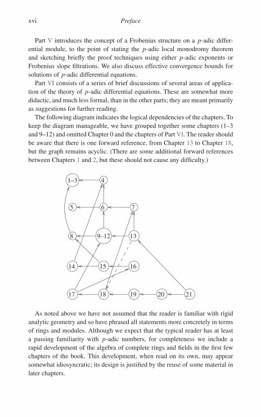
The following diagram indicates the logical dependencies of the chapters. Tokeep the diagram manageable, we have grouped together some chapters (1–3and 9–12) and omitted Chapter 0 and the chapters of Part VI. The reader shouldbe aware that there is one forward reference, from Chapter 13 to Chapter 18,but the graph remains acyclic. (There are some additional forward referencesbetween Chapters 1 and 2, but these should not cause any difficulty.)
�������1–3 �� ����4��
�� ����5 �� ����6��
��
�� ����7��
�� ����8
��
��������9–12��
��
������ !13��
��
�����������
������ !14
��������������������������� ������ !15
��������������� ������ !16��
������ !17
������������������
������������������ ������ !18
����������������������������� ������ !19�� ������ !20�� ������ !21
������������������������
As noted above we have not assumed that the reader is familiar with rigidanalytic geometry and so have phrased all statements more concretely in termsof rings and modules. Although we expect that the typical reader has at leasta passing familiarity with p-adic numbers, for completeness we include arapid development of the algebra of complete rings and fields in the first fewchapters of the book. This development, when read on its own, may appearsomewhat idiosyncratic; its design is justified by the reuse of some material inlater chapters.
Preface xvii
We would like to think that the background needed is that of a two-semesterundergraduate abstract algebra course. However, some basic notions fromcommutative algebra do occasionally intervene, including flat modules, exactsequences, and the snake lemma. It may be helpful to have a well-indexed texton commutative algebra within arm’s reach; we like Eisenbud’s book [84], butthe far slimmer Atiyah and Macdonald [9] should also suffice.
The author would like to thank the participants of the MIT course 18.787(“Topics in number theory”, fall 2007) for numerous comments on the lec-ture notes which ultimately became this book. Particular thanks are due to BenBrubaker and David Speyer for giving guest lectures, and to Chris Davis, Han-sheng Diao, David Harvey, Raju Krishnamoorthy, Ruochuan Liu, Eric Rosen,and especially Liang Xiao for providing feedback. Additional feedback wasprovided by Francesco Baldassarri, Laurent Berger, Bruno Chiarellotto, GillesChristol, Ricardo García López, Tim Gowers, and Andrea Pulita.
During the preparation of the course and of this book, the author was sup-ported by a National Science Foundation CAREER grant (DMS-0545904), aSloan Research Fellowship, MIT’s NEC Research Support Fund, and the MITCecil and Ida Green Career Development Professorship.


0
Introductory remarks
The theory of ordinary differential equations is a fundamental instrument ofcontinuous mathematics, in which the central objects of study are functionsinvolving real numbers. It is not immediately apparent that this theory hasanything useful to say about discrete mathematics in general or number theoryin particular.
In this book we consider ordinary differential equations in which the roleof the real numbers is instead played by the field of p-adic numbers, for someprime number p. The p-adics form a number system with enough formal sim-ilarities to the real numbers to permit meaningful analogues of notions fromcalculus, such as continuity and differentiability. However, the p-adics incor-porate data from arithmetic in a fundamental way; two numbers are p-adicallyclose together if their difference is divisible by a large power of p.
In this chapter, we first indicate briefly some ways in which p-adic differen-tial equations appear in number theory. We then focus on an example of Dwork,in which the p-adic behavior of Gauss’s hypergeometric differential equationrelates to the manifestly number-theoretic topic of the number of points on anelliptic curve over a finite field.
Since this chapter is meant only as an introduction, it is full of statementsfor which we give references instead of proofs. This practice is not typical ofthe rest of this book, except for the discussions in Part VI.
0.1 Why p-adic differential equations?
Although the very existence of a highly developed theory of p-adic ordinarydifferential equations is not entirely well known even within number theory,the subject is actually almost 50 years old. Here are circumstances, past andpresent, in which it arises; some of these will be taken up again in Part VI.
1
2 Introductory remarks
Variation of zeta functions (see Chapter 22). The original circumstance inwhich p-adic differential equations appeared in number theory was Dwork’swork on the variation of zeta functions of algebraic varieties over finite fields.Roughly speaking, solving certain p-adic differential equations can give riseto explicit formulas for the numbers of points on varieties over finite fields.
In contrast with methods involving étale cohomology, methods for study-ing zeta functions based on p-adic analysis (including p-adic cohomology)lend themselves well to numerical computation. The interest in computingzeta functions for varieties where straightforward point-counting is impossible(e.g., curves over extremely large finite fields) has been driven by applica-tions in computer science, the principal example being cryptography based onelliptic or hyperelliptic curves.
p-adic cohomology (see Chapter 23). Dwork’s work suggested, but did notimmediately lead to, a proper analogue of étale cohomology based on p-adicanalytic techniques. Such an analogue was eventually developed by Berth-elot (on the basis of some work of Monsky and Washnitzer, and also ideasof Grothendieck); it is called rigid cohomology (see the notes at the end of thischapter for the origin of the word “rigid”). The development of rigid cohomol-ogy has lagged somewhat behind that of étale cohomology, partly owing to theemergence of some thorny problems related to the construction of a good cate-gory of coefficients. These problems, which have only recently been resolved,are rather closely related to questions concerning p-adic differential equations;in fact, some results presented in this book have been used to address them.
p-adic Hodge theory (see Chapter 24). The subject of p-adic Hodge theoryaims to do for the cohomology of varieties over p-adic fields what ordinaryHodge theory does for the cohomology of varieties over C: that is, it aimsto provide a better understanding of the cohomology of a variety in its ownright, independently of the geometry of the variety. In the p-adic case, thecohomology in question is often étale cohomology, which carries the structureof a Galois representation.
The study of such representations, pioneered by Fontaine, involves a numberof exotic auxiliary rings (rings of p-adic periods), which serve their intendedpurposes but are otherwise a bit mysterious. More recently, the work of Bergerhas connected much of the theory to the study of p-adic differential equations;notably, a key result that was originally intended for use in p-adic cohomol-ogy (the p-adic local monodromy theorem) turned out to imply an importantconjecture about Galois representations, Fontaine’s conjecture on potentialsemistability.
Ramification theory (see Chapter 19). There are some interesting analo-gies between properties of differential equations over C with meromorphic
0.2 Zeta functions of varieties 3
singularities and properties of “wildly ramified” Galois representations ofp-adic fields. At some level, this is suggested by the parallel formulation ofthe Langlands conjectures in the number field and function field cases. Onecan use p-adic differential equations to interpolate between the two situations,by associating differential equations with Galois representations (as in the pre-vious item) and then using differential invariants (for example, irregularity) torecover Galois invariants (for example, Artin and Swan conductors).
For representations of the étale fundamental group of a variety over a fieldof positive characteristic of dimension greater than 1, it is difficult to con-struct meaningful Galois-theoretic numerical invariants. Recent work of Abbesand Saito [1, 2] provides satisfactory definitions, but the resulting quantitiesare quite difficult to calculate. One can alternatively use p-adic differentialequations to define invariants which can be somewhat easier to deal with; forinstance, one can define a differential Swan conductor which is guaranteedto be an integer [133], whereas this is not clearly the case for the Abbes–Saito conductor. One can then equate the two conductors, deducing integralityfor the Abbes–Saito conductor; this has been carried out by Chiarellotto andPulita [40] for one-dimensional representations and by L. Xiao [219] in thegeneral case.
0.2 Zeta functions of varieties
For the rest of this introduction, we return to Dwork’s original example show-ing the role of p-adic differential equations and their solutions in numbertheory. This example refers to elliptic curves, for which see Silverman’s book[200] for background.
Definition 0.2.1. For λ in some field K , let Eλ be the elliptic curve over Kdefined by the equation
Eλ : y2 = x(x − 1)(x − λ)
in the projective plane. Remember that there is one point O = [0 : 1 : 0] atinfinity. There is a natural commutative group law on Eλ(K ), with identityelement O , characterized by the property that three points add to zero if andonly if they are collinear. (It is better to say that three points add to zero ifthey are the three intersections of Eλ with some line, as this correctly permitsdegenerate cases. For instance, if two of the points coincide, the line must bethe tangent to Eλ at that point.)
For elliptic curves over finite fields, one has the following result of Hasse,which generalizes some observations, made by Gauss and others, for certainspecial cases.
4 Introductory remarks
Theorem 0.2.2 (Hasse). Suppose that λ belongs to a finite field Fq . If we write#Eλ(Fq) = q + 1 − aq(λ), then |aq(λ)| ≤ 2
√q.
Proof. See [200, Theorem V.1.1].
Hasse’s theorem was later vastly generalized as follows, originally as a setof conjectures by Weil. (Despite no longer being conjectural, these are stillcommonly referred to as the Weil conjectures.)
Definition 0.2.3. For X an algebraic variety over Fq , the zeta function of X isdefined as the formal power series
ζX (T ) = exp
( ∞∑n=1
T n
n#X (Fqn )
);
another way to write this, which makes it look more like a typical zetafunction, is
ζX (T ) =∏
x
(1 − T deg(x))−1,
where x runs over the Galois orbits of X (Fq) and deg(x) is the size of the orbitx . (If you prefer algebro-geometric terminology, you may run x over closedpoints of the scheme X , in which case deg(x) denotes the degree of the residuefield of x over Fq .)
Example 0.2.4. For X = Eλ one can verify that
ζX (T ) = 1 − aq(λ)T + qT 2
(1 − T )(1 − qT ),
using properties of the Tate module of Eλ; see [200, Theorem V.2.2].
A statement of the Weil conjectures is given in the following theorem.
Theorem 0.2.5 (Dwork, Grothendieck, Deligne, et al.). Let X be an alge-braic variety over Fq . Then ζX (T ) represents a rational function of T .Moreover, if X is smooth and proper of dimension d, we can write
ζX (T ) = P1(T ) · · · P2d−1(T )
P0(T ) · · · P2d(T ),
where each Pi (T ) has integer coefficients, satisfies Pi (0) = 1, and has allroots in C on the circle |T | = q−i/2.
Proof. The proof of this theorem is a sufficiently massive undertaking thateven a reference is not reasonable here; instead, we give [107, Appendix C] asa source of references. (Another useful exposition is [178].)
0.3 Zeta functions and p-adic differential equations 5
Remark 0.2.6. It is worth pointing out that the first complete proof ofTheorem 0.2.5 used the fact that for any prime � �= p one has
#X (Fqn ) =∑
i
(−1)i Trace(Fn, Hiet(X,Q�)),
where Hiet(X,Q�) is the i-th étale cohomology group of X (or rather, the base
change of X to Fq ) with coefficients in Q�. This is an instance of the Lefschetztrace formula in étale cohomology.
0.3 Zeta functions and p-adic differential equations
Remark 0.3.1. The interpretation of Theorem 0.2.5 in terms of étale coho-mology (Remark 0.2.6) is all well and good, but there are several downsides.An important one is that étale cohomology is not explicitly computable; forinstance, it is not straightforward to describe étale cohomology to a computerwell enough that the computer can make calculations. (The main problem isthat while one can write down étale cocycles, it is very hard to tell whether anygiven cocycle is a coboundary.)
Another important downside is that you do not get every good informationabout what happens to ζX when you vary X . This is where p-adic differentialequations enter the picture. It was observed by Dwork that if one has a familyof algebraic varieties defined over Q, the same differential equations appearon the one hand when one studies the variation of complex periods and on theother hand when one studies the variation of zeta functions over Fp.
Here is an explicit example due to Dwork.
Definition 0.3.2. Recall that the hypergeometric series
F(a, b; c; z) =∞∑
i=0
a(a + 1) · · · (a + i)b(b + 1) · · · (b + i)
c(c + 1) · · · (c + i)i ! zi (0.3.2.1)
satisfies the hypergeometric differential equation
z(1 − z)y′′ + (c − (a + b + 1)z)y′ − aby = 0. (0.3.2.2)
Set
α(z) = F(1/2, 1/2; 1; z).
Over C, α is related to an elliptic integral, for instance, by the formula
α(λ) = 2
π
∫ π/2
0
dθ√1 − λ sin2 θ
(0 < λ < 1).

6 Introductory remarks
(One can extend this to complex λ, but care needs to be taken with the branchcuts.) This elliptic integral can be viewed as a period integral for the curve Eλ,i.e., one is integrating some meromorphic differential form on Eλ around someloop (or more properly, around some homology class).
Let p be an odd prime. We now try to interpret α(z) as a function of ap-adic variable rather than a complex variable. Be aware that this means that zcan take any value in a field with a norm extending the p-adic norm on Q, notjust in Qp itself. (For the moment, you can imagine z running over a completedalgebraic closure of Qp.)
Lemma 0.3.3. The series α(z) converges p-adically for |z| < 1.
Proof. Exercise.
Dwork discovered that a closely related function admits a sort of analyticcontinuation.
Definition 0.3.4. Define the Igusa polynomial
H(z) =(p−1)/2∑
i=0
((p − 1)/2
i
)2
zi .
Modulo p, the roots of H(z) are the values of λ ∈ Fp for which Eλ is a super-singular elliptic curve, i.e., for which aq(λ) ≡ 0 (mod p). (In fact, the rootsof H(z) all belong to Fp2 , by a theorem of Deuring; see [200, Theorem V.3.1].)
Dwork’s analytic continuation result is the following.
Theorem 0.3.5 (Dwork). There exists a series ξ(z) = ∑∞i=0 Pi (z)/H(z)i ,
with each Pi (z) ∈ Qp[z], converging uniformly for those z satisfying |z| ≤ 1and |H(z)| = 1 and such that
ξ(z) = (−1)(p−1)/2 α(z)
α(z p)(|z| < 1).
Proof. See [213, §7].
Remark 0.3.6. Note that ξ itself satisfies a differential equation derivedfrom the hypergeometric equation. We will see such equations again oncewe introduce the notion of a Frobenius structure on a differential equation,in Chapter 17.
In terms of the function ξ , we can compute zeta functions in the Legendrefamily as follows.
0.4 A word of caution 7
Definition 0.3.7. Let Zq be the unique unramified extension of Zp with residuefield Fq . For λ ∈ Fq , let [λ] be the unique qth root of 1 in Zq congruent to λmod p (the Teichmüller lift of λ).
Theorem 0.3.8 (Dwork). If q = pa and λ ∈ Fq is not a root of H(z), then
T 2 − aq(λ)T + q = (T − u)(T − q/u),
where
u = ξ([λ])ξ([λ]p) · · · ξ([λ]pa−1).
That is, the quantity u is the “unit root” (meaning the root of valuation 0) ofthe polynomial T 2−aq(λ)T +q occurring (up to reversal) in the zeta function.
Proof. See [213, §7].
0.4 A word of caution
Example 0.4.1. Before we embark on the study of p-adic ordinary differentialequations, a cautionary note is in order concerning the rather innocuous-looking differential equation y′ = y. Over R or C, this equation is nonsingulareverywhere and its solutions y = cex are defined everywhere.
Over a p-adic field, things are quite different. As a power series aroundx = 0, we have
y = c∞∑
n=0
xn
n!and the denominators hurt us rather than helping. In fact, the series only con-verges for |x | < p−1/(p−1) (assuming that we are normalizing in such a waythat |p| = p−1). For comparison, note that the logarithmic series
log1
1 − x=
∞∑n=1
xn
n
converges for |x | < 1.
Remark 0.4.2. The conclusion to be drawn from the previous example is thatthere is no fundamental theorem of ordinary differential equations over thep-adics! In fact, the hypergeometric differential equation in the previous exam-ple was somewhat special; the fact that it had a solution in a disc where it hadno singularities was not a foregone conclusion. One of Dwork’s discoveriesis that this typically happens for differential equations that “come fromgeometry”, such as the Picard–Fuchs equations, which arise from integrals
8 Introductory remarks
of algebraic functions (e.g., elliptic integrals). Another of Dwork’s discoveriesis that, using similar techniques to those used to study obstructions to solvingcomplex differential equations in singular discs, one can quantify the obstruc-tion to solving a p-adic differential equation in a nonsingular disc. We willcarry this out later in the book.
Notes
For detailed notes on the topics discussed in Section 0.1, see the notes for thechapters referenced.
We again mention [107, Appendix C] and [178] as starting points for furtherreading about the Weil conjectures.
The notion of an analytic function specified in terms of a uniform limitof rational functions with poles prescribed to certain regions is the originalsuch notion, introduced by Krasner. For this book, we will restrict our con-sideration of p-adic analysis to working with complete rings in this fashion,without attempting to introduce any notion of nonarchimedean analytic geom-etry. However, it must be noted that it is much better in the long run to workin terms of analytic geometry; for example, it is prohibitively difficult to dealwith partial differential equations without doing so.
That said, there are several ways to develop a theory of analytic spaces over anonarchimedean field. The traditional method is Tate’s theory of rigid analyticspaces, so-called because one develops everything “rigidly” by imitating thetheory of schemes in algebraic geometry but using rings of convergent powerseries instead of polynomials. The canonical foundational reference for rigidgeometry is the book of Bosch, Güntzer, and Remmert [31], but novices mayfind the text of Fresnel and van der Put [93] or the lecture notes of Bosch [30]more readable. A more recent method, which in some ways is more robust,is Berkovich’s theory of nonarchimedean analytic spaces (commonly calledBerkovich spaces), as introduced in [19] and further developed in [20]. Forboth points of view, see also the lecture notes of Conrad [59].
Dwork’s original analysis of the Legendre family of elliptic curves usingthe associated hypergeometric equation (this analysis expands earlier work ofTate) appears in [74, §8]. The treatment in [213] is more overtly related top-adic cohomology.
The family of hypergeometric equations with a, b, c ∈ Q∩Zp is rich enoughthat one could devote an entire book to the study of its p-adic properties.Indeed, Dwork did exactly this; the result was [78].
It is possible to resurrect in part the fundamental theorem of ordinary dif-ferential equations in the p-adic setting. The best results in that direction seem
Exercises 9
to be those of Priess-Crampe and Ribenboim [183]. One consequence of theirwork is the fact that a differential equation over Qp has a solution if and onlyif it has a sufficiently good approximate solution; this amounts to a differen-tial version of Hensel’s lemma. We too will need noncommutative forms ofHensel’s lemma; see Theorem 2.2.2.
Christol [45] has given an interesting retrospective on some of the keyideas of Dwork, including generic points, the transfer principle, and Frobeniusstructures, which resonate throughout this book.
Exercises
The reader new to p-adic numbers should postpone doing these exercises untilhe or she has read Part I.(1) Prove directly from the definition that the series F(a, b; c; z) converges
p-adically for |z| < 1 whenever a, b, c are rational numbers withdenominators not divisible by p. This implies Lemma 0.3.3.
(2) Using the fact that α(z) satisfies the hypergeometric equation, write downa nontrivial differential equation with coefficients in Q(z) satisfied by thefunction ξ(z).
(3) Check that the usual formula
lim infn→∞ |an|−1/n
for the radius of convergence of the power series∑∞
n=0 anzn still worksover a nonarchimedean field. That is, the series converges when |z| is lessthan this radius and diverges when |z| is greater than this radius.
(4) Show that in the previous exercise, just like in the archimedean case, apower series over a nonarchimedean field can either converge or diverge ata value of z for which |z| equals the radius of convergence.
(5) Check that (as claimed in Example 0.4.1), under the normalization|p| = p−1, the exponential series exp(z) over Qp has radius of con-vergence p−1/(p−1), while the logarithm series log(1 − z) has radius ofconvergence 1.
(6) Show that, over Qp, while a power series in z which converges for |z| ≤ 1may have an antiderivative which only converges for |z| < 1, its derivativestill converges for |z| ≤ 1. This is the reverse of what happens over anarchimedean field.

Part I
Tools of p-adic Analysis


1
Norms on algebraic structures
In this chapter, we recall some basic facts about norms (absolute values),primarily of the nonarchimedean sort, on groups, rings, fields, and modules.We also briefly discuss the phenomenon of spherical completeness, which ispeculiar to the nonarchimedean setting. Our discussion is not particularly com-prehensive; the reader new to nonarchimedean analysis is directed to [191] fora fuller treatment.
Several proofs in this chapter make forward references to Chapter 2.There should be no difficulty in verifying the absence of circularreferences.
Convention 1.0.1. In this book, a ring means a commutative ring unless com-mutativity is suppressed explicitly by describing the ring as “not necessarilycommutative” or implicitly by its usage in certain phrases, e.g., a ring oftwisted polynomials (Definition 5.5.1).
Notation 1.0.2. For R a ring, we denote by R× the multiplicative group ofunits of R.
1.1 Norms on abelian groups
Let us start by recalling some basic definitions from analysis, before specializ-ing to the nonarchimedean case.
Definition 1.1.1. Let G be an abelian group. A seminorm (or semiabsolutevalue) on G is a function | · | : G → [0,+∞) satisfying the followingconditions.
13

14 Norms on algebraic structures
(a) We have |0| = 0.(b) For f, g ∈ G, | f − g| ≤ | f | + |g|. (Equivalently, |g| = |−g| and | f +
g| ≤ | f |+ |g|. This condition is usually called the triangle inequality.)We say that the seminorm | · | is a norm (or absolute value) if the followingadditional condition holds.
(a′) For g ∈ G, |g| = 0 if and only if g = 0.We also express this by saying that G is separated under | · |. A seminorm onan abelian group G induces a metric topology on G, in which the basic opensubsets are the open balls, i.e., sets of the form {g ∈ G : | f − g| < r} for somef ∈ G and some r > 0.
Definition 1.1.2. Let G,G ′ be abelian groups equipped with seminorms | · |,| · |′, respectively, and let φ : G → G ′ be a homomorphism. Note that φis continuous for the metric topologies on G,G ′ if and only if there exists afunction h : (0,+∞)→ (0,+∞) such that for all r > 0,
{g ∈ G : |g| < h(r)} ⊆ {g ∈ G : |φ(g)|′ < r}.We say that φ is bounded if there exists c ≥ 0 such that |φ(g)|′ ≤ c|g| forall g ∈ G. We say that φ is isometric if |φ(g)|′ = |g| for all g ∈ G. We saytwo seminorms | · |1, | · |2 on G are topologically equivalent if they inducethe same metric topology, i.e., the identity morphism on G is continuous inboth directions. We say that | · |1, | · |2 are metrically equivalent if there existc1, c2 > 0 such that, for all g ∈ G,
|g|1 ≤ c1|g|2, |g|2 ≤ c2|g|1;this implies topological equivalence but the reverse implication does notnecessarily hold.
Definition 1.1.3. Let G be an abelian group equipped with a seminorm.A Cauchy sequence in G under | · | is a sequence {xn}∞n=0 in G such that,for any ε > 0, there exists an integer N such that, for all integers m, n ≥ N ,|xm −xn| < ε. We say the sequence {xn}∞n=0 is convergent if there exists x ∈ Gsuch that, for any ε > 0 there exists an integer N such that, for all integersn ≥ N , |x − xn| < ε; in this case, the sequence is automatically Cauchy, andwe say that x is a limit of the sequence. If G is separated under | · |, then limitsare unique when they exist. We say G is complete under | · | if every Cauchysequence has a unique limit.
Theorem 1.1.4. Let G be an abelian group equipped with a norm | · |. Thenthere exists an abelian group G ′, equipped with a norm | · |′ under which it iscomplete, and an isometric homomorphism φ : G → G ′ with dense image.
This is standard, so we only sketch the proof.

1.1 Norms on abelian groups 15
Proof. We take the set of Cauchy sequences in G and declare two sequences{xn}∞n=0, {yn}∞n=0 to be equivalent if the sequence x0, y0, x1, y1, . . . is alsoCauchy. This is easily shown to be an equivalence relation; let G ′ be the setof equivalence classes. It is then straightforward to construct the group oper-ation (termwise addition) and the norm on G ′ (the limit of the norms of theterms of the sequence). The map φ takes g ∈ G to the constant sequenceg, g, . . .
Definition 1.1.5. With the notation of Theorem 1.1.4, we call G ′ the comple-tion of G; the group G ′, equipped with the norm | · |′ and the homomorphismφ, is functorial in G. That is, any continuous homomorphism G → H extendsuniquely to a continuous homomorphism G ′ → H ′ between the completions;in particular, G ′ is unique up to unique isomorphism. Note that one can alsodefine the completion even if G is only equipped with a seminorm, but only byfirst quotienting by the kernel of the seminorm; in that case, the map from Gto its completion need not be injective.
Definition 1.1.6. If R is a not necessarily commutative ring and | · | is a semi-norm on its additive group, we say that | · | is submultiplicative if the followingadditional condition holds.
(c) For f, g ∈ R, | f g| ≤ | f ||g|.We say that | · | is multiplicative if the following additional condition holds.
(c′) For f, g ∈ R, | f g| = | f ||g|.The completion of a ring R equipped with a submultiplicative seminormadmits a natural ring structure, because the termwise product of two Cauchysequences is again Cauchy.
Lemma 1.1.7. Let F be a field equipped with a multiplicative norm. Then thecompletion of F is also a field.
Proof. Note that if { fn}∞n=0 is a Cauchy sequence in F then {| fn|}∞n=0 is aCauchy sequence in R by the triangle inequality, and so has a limit since R
is complete. Since F is equipped with a true norm, if { fn}∞n=0 does not con-verge to 0 then {| fn|}∞n=0 also must not converge to 0. In particular, | fn|∞n=0 isbounded below away from 0, from which it follows easily that { f −1
n }∞n=0 is alsoa Cauchy sequence. This proves that every nonzero element of the completionof F has a multiplicative inverse, as desired.
Proposition 1.1.8. Two multiplicative norms | · |, | · |′ on a field F are topo-logically equivalent if and only if there exists c > 0 such that |x |′ = |x |c forall x ∈ F.
Proof. Exercise, or see [80, Lemma I.1.2].
16 Norms on algebraic structures
Definition 1.1.9. Let G be an abelian group equipped with a seminorm | · |G ,and let G ′ be a subgroup of G. The quotient seminorm on the quotient G/G ′is defined by the formula
|g + G ′|G/G ′ = infg′∈G ′{|g + g′|G}. (1.1.9.1)
If | · |G is a norm, then | · |G/G ′ is a norm if and only if G ′ is closed in G.
1.2 Valuations and nonarchimedean norms
We now restrict our attention to nonarchimedean absolute values, which canbe described additively (using valuations) as well as multiplicatively (usingnorms). It will be convenient to switch back and forth between these points ofview throughout the book.
Definition 1.2.1. A real semivaluation on an abelian group G is a functionv : G → R ∪ {+∞} with the following properties.
(a) We have v(0) = +∞.(b) For f, g ∈ G, v( f − g) ≥ min{v( f ), v(g)}.
We say v is a real valuation if the following additional condition holds.(a′) For g ∈ G, v(g) = +∞ if and only if g = 0.
If v is a real (semi)valuation on G, then the function | · | = e−v(·) is a(semi)norm on G which is nonarchimedean (or ultrametric), i.e., it satisfiesthe strong triangle inequality, which is given as follows.
(b′) For f, g ∈ G, | f − g| ≤ max{| f |, |g|}.Conversely, for any nonarchimedean (semi)norm | · |, v(·) = − log | · | is areal (semi)valuation. We will apply various definitions made for seminormsto semivaluations in this manner; for instance, if R is a ring and v is a real(semi)valuation on its additive group, we say that v is (sub)multiplicative if thecorresponding nonarchimedean (semi)norm is.
Definition 1.2.2. We say that a group is nonarchimedean if it is equippedwith a nonarchimedean norm; we say that a ring or field is nonarchimedeanif it is equipped with a multiplicative nonarchimedean norm. Note that anynonarchimedean ring is an integral domain.
Definition 1.2.3. Let F be a nonarchimedean field. The multiplicative valuegroup of a nonarchimedean field F is the image of F× under | · |, viewed asa subgroup of R+; we will often denote it simply as |F×|. The additive valuegroup of F is the set of negative logarithms of the multiplicative value group.If these groups are discrete and nonzero (i.e., isomorphic to Z), we say F isdiscretely valued. Define also
1.3 Norms on modules 17
oF = { f ∈ F : v( f ) ≥ 0},mF = { f ∈ F : v( f ) > 0},κF = oF/mF .
Note that oF is a local ring (the valuation ring of F), mF is the maximal idealof oF , and κF is a field (the residue field of F).
It is worth noting that there are comparatively few archimedean (i.e., notnonarchimedean) absolute values on fields.
Theorem 1.2.4 (Ostrowski). Let F be a field equipped with a norm | · |. Then| · | fails to be nonarchimedean if and only if the sequence |1|, |2|, |3|, . . . isunbounded. In that case, F is isomorphic to a subfield of C equipped with therestriction of the usual absolute value.
Proof. Exercise, or see [191, §2.1.6] and [191, §2.2.4], respectively.
1.3 Norms on modules
When considering norms on modules, we usually require compatibility withthe underlying ring.
Definition 1.3.1. Let R be a ring equipped with a multiplicative seminorm | · |,and let M be an R-module equipped with a seminorm | · |M . We say that | · |Mis compatible with | · | (or with R) if the following conditions hold.
(a) For f ∈ R, x ∈ M , | f x |M = | f ||x |M .(b) If | · | is nonarchimedean, then so is | · |M .
Note that (b) is not superfluous; see the end-of-chapter exercises. If R is a field,then two norms | · |M , | · |′M on M compatible with R are metrically equivalentif and only if they are topologically equivalent (exercise).
One thing to be aware of is that if M ′ is a quotient of M and | · |M ′ is thequotient norm on M ′ induced by | · |M , then in general we cannot say that | · |M ′is compatible with R. Rather, we only have the inequality
| f x ′|M ′ ≤ | f ||x ′|M ′ ( f ∈ R, x ′ ∈ M ′);this implies compatibility only if R is a field.
We can generate a rich supply of norms on modules via the followingconstruction.
Definition 1.3.2. Let R be a ring equipped with a multiplicative (semi)norm| · |, and let M be a finite free R-module. For B a basis of M , define thesupremum (semi)norm of M with respect to B by setting
18 Norms on algebraic structures
∣∣∣∣∣∑b∈B
cbb
∣∣∣∣∣ = supb∈B
{|cb|} (cb ∈ R).
This (semi)norm extends canonically to M ⊗R S for any isometric inclusionR ↪→ S. (The situation is more complicated for arbitrary (semi)norms; seeDefinition 1.3.10 below.)
We say that a seminorm on M is supremum-equivalent if it is metricallyequivalent to the supremum seminorm with respect to some basis; the same isthen true of any basis, by Lemma 1.3.3 below. In particular, if | · | is a normthen any supremum-equivalent seminorm is a norm.
Lemma 1.3.3. Let R be a ring equipped with a multiplicative seminorm | · |,and let M be a finite free R-module. Then for any two bases B1, B2 of M, thesupremum seminorms of M defined by B1 and B2 are metrically equivalent.
Proof. Put B1 = {m1,1, . . . ,m1,n} and B2 = {m2,1, . . . ,m2,n}. Define then × n matrix A over R by the formula
m2, j =n∑
i=1
Ai j m1,i ;
then A is invertible. In particular, we cannot have |Ai j | = 0 for all i, j .For x ∈ M , we can uniquely write x = a1,1m1,1 + · · · + a1,nm1,n =
a2,1m2,1 + · · · + a2,nm2,n with ai, j ∈ R. We then have
a1,i =n∑
j=1
Ai j a2, j (i = 1, . . . , n)
and so
maxi
{|a1,i |} ≤⎛⎝ n∑
i=1
n∑j=1
|Ai j |⎞⎠max
j{|a2, j |}.
This inequality, together with the corresponding one with the bases reversed(involving the matrix A−1), implies the claim.
Corollary 1.3.4. Let R ↪→ S be an isometric inclusion of rings equippedwith multiplicative seminorms. Let M be a finite free R-module. Let | · |Mbe a seminorm on M that is compatible with R, which is the restriction of asupremum-equivalent seminorm on M ⊗R S that is compatible with S. Then| · |M is supremum-equivalent.
Proof. Put N = M ⊗R S, and let | · |N be a supremum-equivalent norm onN , compatible with S, whose restriction to M equals | · |M . Pick any basis B
1.3 Norms on modules 19
of M ; then B is also a basis of N . Since | · |N is equivalent to the supremumnorm on N defined by some basis, by Lemma 1.3.3 it is also equivalent to thesupremum norm defined by B. By restriction, we see that | · |M is equivalent tothe supremum norm on M defined by B.
The notion of supremum-equivalence is well-behaved under quotients.
Lemma 1.3.5. Let R be a ring equipped with a multiplicative seminorm | · |,let M be a finite free R-module, and let M1 be a finite free R-submodule of Msuch that M/M1 is also free. Let | · |M be a supremum-equivalent norm on Mcompatible with R. Then the quotient norm | · |M1 on M1 induced by | · |M isalso supremum-equivalent.
Proof. Let m1, . . . ,mk be a basis of M1, and choose mk+1, . . . ,mn ∈ M lift-ing a basis of M/M1. Then m1, . . . ,mn is a basis of M ; by Lemma 1.3.3, | · |Mis equivalent to the supremum norm defined by m1, . . . ,mn . That is, there existc1, c2 > 0 such that, for any x = a1m1 + · · · + anmn ∈ M ,
c1 max{|a1|, . . . , |an|} ≤ |x |M ≤ c2 max{|a1|, . . . , |an|}.Then for any ak+1, . . . , an ∈ R, we have
c1 max{|ak+1|, . . . , |an|} = c1 infa1,...,ak∈R
{max{|a1|, . . . , |an|}}≤ inf
a1,...,ak∈R{|a1m1 + · · · + anmn|M }
= |ak+1mk+1 + · · · + anmn|M1
≤ |ak+1mk+1 + · · · + anmn|M≤ c2 max{|ak+1|, . . . , |an|}.
Thus | · |M1 is equivalent to the supremum norm defined by the images ofmk+1, . . . ,mn in M1, proving the desired result.
In general, even over a field, not every compatible norm on a vector spaceneed be supremum-equivalent; see the exercises. However, such supremum-equivalence is true for complete fields.
Theorem 1.3.6. Let F be a field complete for a norm | · |, and let V be afinite-dimensional vector space over F. Then any two norms on V compatiblewith F are metrically equivalent.
Proof. In the archimedean case, apply Theorem 1.2.4 to deduce that F = R
or F = C, then use compactness of the unit ball. In the nonarchimedean case,we proceed as follows. (See [80, Theorem I.3.2] for a different proof.)
20 Norms on algebraic structures
We proceed by induction on n, the case n = 1 being trivial. Let m1, . . . ,mn
be any basis of V . It suffices to show that any given norm | · | on V compat-ible with F is equivalent to the supremum norm defined by m1, . . . ,mn . Oneinequality is evident: for any a1, . . . , an ∈ F , we have
|a1m1 + · · · + anmn|V ≤ maxi
{|mi |}maxi
{|ai |}.
Put V ′ = V/Fm1. Let | · |V ′ denote the quotient seminorm on V ′ inducedby | · |V . This seminorm is compatible with F , but we must check that it isindeed a norm. Suppose on the contrary that a2, . . . , an ∈ F are such that|a2m2 + · · · + anmn|V ′ = 0. Then we can choose a sequence a1,1, a1,2, . . .
of elements of F such that |a1,i m1 + a2m2 + · · · + anmn|V → 0 as i → ∞.But then |a1,i − a1, j ||m1|V = |(a1,i − a1, j )m1|V → 0 as i, j → ∞, so thea1,i form a Cauchy sequence. Since F is complete, this Cauchy sequence hasa limit a1, and |a1m1 + · · · + anmn|V = 0 contrary to the hypothesis that | · |Vis a norm.
Hence | · |V ′ is indeed a norm. By the induction hypothesis, there existsc2 > 0 such that
|a2m2 + · · · + anmn|V ′ ≥ c2 maxi
{|ai |}.We then have
|a1m1 + · · · + anmn|V ≥ max{|a1m1|V , |a2m2 + · · · + anmn|V }≥ max{|a1m1|V , |a2m2 + · · · + anmn|V ′ }≥ min{|m1|, c2}max
i{|ai |},
proving that | · |V is equivalent to the supremum norm defined by m1, . . . ,mn .
Even if a norm is supremum-equivalent, it need not be equal to the supre-mum norm defined by any basis. However, one can approximate supremum-equivalent norms using supremum norms as follows. For a stronger result inthe spherically complete case, see Lemma 1.5.5.
Lemma 1.3.7 (Approximation lemma). Let F be a nonarchimedean field, letV be a finite-dimensional vector space over F, and let | · |V be a supremum-equivalent norm on V compatible with F. Assume that either:
(a) c > 1 and the value group of F is not discrete; or(b) c ≥ 1 and the value groups of F and V coincide and are discrete.
Then there exists a basis of V defining a supremum norm | · |′V for which
c−1|x |V ≤ |x |′V ≤ c|x |V (x ∈ V ).
1.3 Norms on modules 21
Proof. We induct on n, with trivial base case n = 0. For n > 0, pick anynonzero m1 ∈ V , and put V1 = V/Fm1. Using (a) or (b), we can rescale m1
by an element of F to force 1 ≤ |m1|V ≤ c2/3.Equip V1 with the quotient seminorm |·|V1 induced by |·|V . By Lemma 1.3.5,
| · |V1 is again supremum-equivalent. Moreover, in case (b) the infimum in(1.1.9.1) is always achieved, i.e., for every x1 ∈ V1, there exists x ∈ V liftingx1 with |x |V = |x1|V1 . Hence V1 again satisfies (b).
We may now apply the induction hypothesis to V1 to produce a basism2,1, . . . ,mn,1 of V1 defining a supremum norm | · |′V1
for which
c−1/3|x1|V1 ≤ |x1|′V1≤ c1/3|x1|V1 (x1 ∈ V1).
For i = 2, . . . , n, choose mi ∈ V lifting mi,1 such that |mi |V ≤ c1/3|mi,1|V1 ;then
|mi |V ≤ c1/3|mi,1|V1 ≤ c2/3|mi,1|′V1= c2/3.
Let | · |′V be the supremum norm defined by m1, . . . ,mn . For x ∈ V , writex = a1m1 + · · · + anmn with ai ∈ F . On the one hand,
|x |V ≤ max1≤i≤n
{|ai ||mi |V } ≤ c2/3|x |′V .On the other hand, if x1 is the image of x in V1 then
|x1|′V1≤ c1/3|x1|V1 ≤ c1/3|x |V ,
so |a2|, . . . , |an| ≤ c1/3|x |V . Moreover,
|a1m1|V ≤ max{|x |V , |x − a1m1|V }≤ max{|x |V , c2/3|x − a1m1|′V }= max{|x |V , c2/3 max{|a2|, . . . , |an|}}≤ c|x |V .
Since |m1|V ≥ 1, we deduce |a1| ≤ c|x |V and so |x |′V ≤ c|x |V . This provesthe desired inequalities.
We need the following infinite-dimensional analogue of Theorem 1.3.6,taken from [195, Proposition 10.4]. Be aware that the situation in the archi-medean case is much subtler; see the notes at the end of the chapter.
Lemma 1.3.8. Let F be a complete nonarchimedean field. Let V be anF-vector space equipped with a norm | · |V compatible with F. Supposethat V contains a dense F-subspace of countable infinite dimension over F.Then there exists a sequence m1,m2, . . . of elements of V with the followingproperties.
22 Norms on algebraic structures
(a) For each m ∈ V , there is a unique sequence a1, a2, . . . of elements ofF such that the series
∑∞i=1 ai mi converges to m.
(b) With notation as in (a), the function | · |′V defined by
|m|′V = supi{|ai mi |V }
is a norm on V compatible with F and metrically equivalent to | · |V .
Proof. Choose an ascending sequence of F-subspaces 0 = V0 ⊂ V1 ⊂ · · · ,with dimF Vn = n, whose union is dense in V . For each n > 0, pick somemn,0 ∈ Vn \ Vn−1.
Let | · |n be the quotient seminorm on V/Vn induced by | · |V . As in theproof of Theorem 1.3.6, we may show by induction on n that | · |n is a norm,as follows. The claim for n = 0 is given. Supposing that | · |n−1 is a norm,let m ∈ V be an element with |m|n = 0. There must exist a sequence ai ofelements of F with |ai mn,0 + m|n−1 → 0 as i → ∞. Since |mn,0|n−1 �= 0by the induction hypothesis, the ai must form a Cauchy sequence in F whoselimit a satisfies |amn,0 + m|n−1 = 0. Again by the induction hypothesis, mand −amn,0 represent the same class in V/Vn−1, so m represents the zeroclass in V/Vn . Hence | · |n is a norm.
Choose an increasing sequence of real numbers 0 < r1 < r2 < · · · < 1.Since | · |n−1 is a norm, we have |mn,0|n−1 �= 0. We can thus choose mn ∈mn,0 + Vn−1 with m1 = m1,0 and
|mn|n−1 = |mn,0|n−1 ≥ rn
rn+1|mn|V (n > 1).
For m ∈ Vn−1 and a ∈ F , we have |amn + m|V ≥ |amn|n−1 ≥(rn/rn+1)|amn|V . If |amn|V = |m|V , this yields
|amn + m|V ≥ rn
rn+1max{|amn|V , |m|V };
the same holds if |amn|V �= |m|V since in that case |amn + m|V = max{|amn|V , |m|V }.
By induction on n, we deduce that, for a1, . . . , an ∈ F ,
|a1m1 + · · · + anmn|V ≥ r1
rn+1max{|a1m1|V , . . . , |anmn|V }
≥ r1 max{|a1m1|V , . . . , |anmn|V }.Combining this with the evident inequality
|a1m1 + · · · + anmn|V ≤ max{|a1m1|V , . . . , |anmn|V },
1.3 Norms on modules 23
we conclude that on ∪n Vn the seminorms | · |V and | · |′V are metrically equiv-alent. Consequently, | · |′V extends by continuity to a function on V which ismetrically equivalent to | · |V and hence is a norm (which is evidently com-patible with F). This assertion will imply both (a) and (b) as soon as we haveestablished the existence aspect of (a), which we will do now.
Given m ∈ V , by hypothesis there exists a sequence x1, x2, . . . of elementsof ∪n Vn converging to m. For j = 1, 2, . . . write x j = ∑∞
i=1 ai, j mi , whereonly finitely many ai, j are nonzero. Since {x j }∞j=1 is a Cauchy sequence, foreach ε > 0 there exists N such that, for j, j ′ ≥ N , |x j − x j ′ |V ≤ ε. Since | · |′Vis metrically equivalent to | · |V , for each ε > 0 there also exists N such that,for j, j ′ ≥ N , |x j − x j ′ |′V ≤ ε.
On the one hand this implies that, for each fixed i , the sequence {ai, j }∞j=1is Cauchy. Since F is complete, this sequence has a limit ai . On the otherhand, for j = N there exists some i0 such that ai, j = 0 for all i ≥ i0. If wewrite xi, j = ∑∞
h=i+1 ah, j m j , for all j ≥ N and all i ≥ i0 we have |xi, j |′V ≤ε and hence |xi, j |V ≤ ε. For fixed i , xi, j converges to m − a1m1 − · · · −ai mi as j → ∞; hence, for all i ≥ i0, |m − a1m1 − · · · − ai mi |V ≤ ε sothe series
∑∞i=1 ai mi converges to m. As noted earlier, both (a) and (b) now
follow.
Definition 1.3.9. For F a field complete for a norm | · |, a Banach space overF is a vector space V over F equipped with a norm compatible with | · |, underwhich it is complete. For V a Banach space and W a closed subspace, thequotient V/W is again complete. See [214] or [195] for a full development ofthe theory of Banach spaces and other topological vector spaces over completenonarchimedean fields.
Definition 1.3.10. Let R be a nonarchimedean ring, and let M, N be modulesover R equipped with seminorms | · |M , | · |N compatible with R. The productseminorm on M ⊗R N is defined by the formula
|x |M⊗R N = inf
{max
1≤i≤s{|mi |M |ni |N } : x =
s∑i=1
mi ⊗ ni
}.
As in the case of the quotient seminorm, it is clear that the product seminorm isa seminorm, but it is not clear whether it is compatible with R unless R happensto be a field. Moreover for norms | · |M and | · |N , it is not clear whether theproduct seminorm is a norm. However, if M and N are finite free R-modulesequipped with supremum-equivalent norms then the product seminorm willbe supremum-equivalent, which forces it to be a norm. See also the followinglemma.

24 Norms on algebraic structures
Lemma 1.3.11. Let F be a complete nonarchimedean field. Let V and W be(possibly infinite-dimensional) vector spaces over F equipped with norms | · |Vand |·|W compatible with F. Then the product seminorm on V ⊗F W is a norm.
Proof. Suppose first that V admits a dense F-subspace of at most countablyinfinite dimension. Then by Theorem 1.3.6 and/or Lemma 1.3.8, we can finda (finite or infinite) sequence m1,m2, . . . of elements of V such that everyelement can be uniquely written as a convergent series
∑∞i=1 ai mi , with ai ∈
F , and | · |V is equivalent to the norm | · |′V defined by∣∣∣∣∣∞∑
i=1
ai mi
∣∣∣∣∣′
V
= supi{|ai mi |V } (ai ∈ F).
More precisely, we have c|·|′V ≤ |·|V ≤ |·|′V for some c > 0. Let π j : V → Fbe the projection carrying
∑∞i=1 ai mi to a j . By tensoring with W , we obtain a
projection π j,W : V ⊗F W → W . For x ∈ V ⊗F W , we define
|x |′V⊗F W = supj{|m j |V |π j,W (x)|W }.
This gives a norm by the following argument. Let∑s
k=1 yk ⊗ zk be anyrepresentation of x ∈ V ⊗F W with yk ∈ V and zk ∈ W , so that
π j,W (x) =s∑
k=1
π j (yk)zk .
Suppose that |x |′V⊗F W = 0; then choose the representation of x to minimizes. If s > 0 then yk �= 0 for all k and the zk must be linearly independent overF . We can then choose j and k such that π j (yk) �= 0, but then
0 = π j,W (x) =s∑
k=1
π j (yk)zk,
a contradiction. Hence s = 0 and so x = 0.For x = ∑s
k=1 yk ⊗ zk ∈ V ⊗F W and any positive integer N , we canexpress x also as
m1⊗π1,W (x)+· · ·+m N ⊗πN ,W (x)+s∑
k=1
(yk − π1(yk)m1 − · · · − πN (yk)m N )⊗zk;
as N → ∞, the product seminorm of the sum over k tends to zero. We thusconclude that, on the one hand,
|x |V⊗F W ≤ |x |′V⊗F W .

1.4 Examples of nonarchimedean norms 25
On the other hand,
maxk
{|yk |V |zk |W } ≥ c supj
maxk
{|π j (yk)m j |V |zk |W }
≥ c supj
{|m j |V
∣∣∣∣∣s∑
k=1
π j (yk)zk
∣∣∣∣∣W
}= c sup
j{|m j |V |π j,W (x)|W },
so that
|x |V⊗F W ≥ c|x |′V⊗F W .
That is, the product seminorm is equivalent to | · |′V⊗F W and so is a norm.In the general case, suppose on the contrary that x = ∑s
j=1 m j ⊗ n j ∈V⊗F W had product seminorm 0. This would mean that we can find a sequencexi ∈ V ⊗F W in which each xi can be represented as
∑sij=1 mi, j ⊗ni, j , and so
limi→∞ max
j{|mi, j |V |ni, j |W } = 0.
Then the same data would be available if we replaced V by the closure of theF-subspace spanned by the m j and the mi, j , and similarly for W . We may thusapply the previous case to obtain a contradiction.
1.4 Examples of nonarchimedean norms
Example 1.4.1. For any field F , there is a trivial norm of F defined by
| f |triv ={
1 f �= 0,
0 f = 0.
This norm is nonarchimedean, and F is complete under it. The trivial case willalways be allowed unless explicitly excluded; it is often a useful input into ahighly nontrivial construction, as in the next few examples.
Example 1.4.2. Let F be any field, and let F((t)) denote the field of formalLaurent series. The t-adic valuation vt on F is defined as follows: for f =∑
i ci t i ∈ F((t)), vt ( f ) is the least i for which ci �= 0. This exponentiates togive a t-adic norm under which F((t)) is complete and discretely valued. (SeeExample 1.5.8 for a variation on this construction.)
Before introducing our next example, we make a more general definition forlater use.
26 Norms on algebraic structures
Definition 1.4.3. Let R be a ring equipped with a nonarchimedean submulti-plicative (semi)norm | · |. For ρ ≥ 0, define the ρ-Gauss (semi)norm | · |ρ onthe polynomial ring R[T ] by∣∣∣∣∣∑
i
Pi Ti
∣∣∣∣∣ρ
= maxi
{|Pi |ρi };
it is clearly submultiplicative. Moreover, it is also multiplicative if | · | is;however, we will postpone the verification of this to the next chapter (seeProposition 2.1.2). For r ∈ R, we define the r-Gauss (semi)valuation vr asthe (semi)valuation associated with the e−r -Gauss (semi)norm.
Remark 1.4.4. The definition of the ρ-Gauss norm depends on the choice ofthe indeterminate T ; that is, it is not equivariant for arbitrary endomorphismsof the ring R[T ]. For clarity, we will sometimes need to specify that the Gaussnorm is being defined with respect to a particular indeterminate.
Example 1.4.5. For F a nonarchimedean field and ρ > 0, the ρ-Gauss normon F[t] (with respect to t) is a multiplicative norm, so it extends to the rationalfunction field F(t). Note that F(t) is discretely valued under the ρ-Gauss normif and only if either:
(a) F carries the trivial norm and ρ �= 1; or(b) F is discretely valued and ρ belongs to the divisible closure of the
multiplicative value group of F .In case (a) the ρ-Gauss norm is equivalent to the t-adic norm if 0 < ρ < 1, tothe trivial norm if ρ = 1, and to the t−1-adic norm if ρ > 1.
So far we have not mentioned the principal examples from number theory;let us do so now.
Example 1.4.6. For p a prime number, the p-adic norm | · |p on Q is definedas follows. Given f = r/s with r, s ∈ Z, write r = pam and s = pbn withm, n not divisible by p and then put
| f |p = p−a+b.
In particular, we have normalized in such a way that |p|p = p−1; this conven-tion is usually taken in order to make the product formula hold. Namely, forany f ∈ Q, if | · |∞ denotes the usual archimedean absolute value then
| f |∞∏
p
| f |p = 1.
Completing Q under | · |p gives the field of p-adic numbers Qp; it is discretelyvalued. Its valuation ring is denoted Zp and called the ring of p-adic integers.

1.4 Examples of nonarchimedean norms 27
Remark 1.4.7. When converting the p-adic norm into a valuation, it is com-mon practice to use base-p logarithms. We have instead opted to keep thefactor of log p visible when we take logarithms. One may liken this practiceto using metric units rather than normalizing some dimensioned constants to 1(e.g., the speed of light).
Just as the only archimedean norm on Q is the usual one, every nontrivialnonarchimedean norm on Q is essentially a p-adic norm, again by a theoremof Ostrowski.
Theorem 1.4.8 (Ostrowski). Any nontrivial nonarchimedean norm on Q isequivalent to the p-adic norm for some prime p.
Proof. See [191, §2.2.4].
To equip extensions of Qp with norms, we use the following result. As usual,when E is a finite extension of a field F we write [E : F] for the degree of thefield extension, i.e., the dimension of E as an F-vector space.
Theorem 1.4.9. Let F be a complete nonarchimedean field. Then any finiteextension E of F admits a unique extension of | · | to a norm on E (underwhich E is also complete).
Proof. We only prove uniqueness now; existence will be established inSection 2.3. Let |·|1 and |·|2 be two extensions of |·| to norms on E . Then thesein particular give norms on E viewed as an F-vector space; by Theorem 1.3.6,these norms are metrically equivalent; that is, there exist c1, c2 > 0 such that
|x |1 ≤ c1|x |2, |x |2 ≤ c2|x |1 (x ∈ E).
They are also both metrically equivalent to the supremum norm for some basisof E over F , under which E is evidently complete.
We now use the extra information that | · |1 and | · |2 are multiplicative(because they are norms on E as a field in its own right). For any positiveinteger n, we may substitute xn in place of x in the previous inequalities andthen take nth roots, to obtain
|x |1 ≤ c1/n1 |x |2, |x |2 ≤ c1/n
2 |x |1 (x ∈ E).
Taking limits as n → ∞ gives |x |1 = |x |2, as desired.
Remark 1.4.10. The completeness of F is crucial in Theorem 1.4.9. Forinstance, the 5-adic norm on Q extends in two different ways to the Gaussianrational numbers Q(i), depending on whether |2 + i | = 5−1 and |2 − i | = 1,or vice versa.
28 Norms on algebraic structures
Because of the uniqueness in Theorem 1.4.9, it also follows that any alge-braic extension E of F , finite or not, inherits a unique extension of | · |.However, if [E : F] = ∞ then E is not complete, so we may prefer to use itscompletion instead. For instance, if F = Qp, we define Cp to be the comple-tion of an algebraic closure of Qp. One might worry that this may launch usinto an endless cycle of completion and algebraic closure, but fortunately thisdoes not occur.
Theorem 1.4.11. Let F be an algebraically closed nonarchimedean field.Then the completion of F is also algebraically closed.
For the proof, see Section 2.3.
1.5 Spherical completeness
For nonarchimedean fields there is an important distinction between two dif-ferent notions of completeness, which does not appear in the archimedeancase.
Definition 1.5.1. A metric space is complete if any decreasing sequence ofclosed balls with radii tending to 0 has nonempty intersection. (For an abeliangroup equipped with a norm this reproduces our earlier definition.) A met-ric space is spherically complete if any decreasing sequence of closed balls,regardless of radii, has nonempty intersection.
Example 1.5.2. The fields R and C with their usual absolute value arespherically complete. Any complete nonarchimedean field which is discretelyvalued, e.g., Qp or C((t)), is spherically complete. Any finite-dimensional vec-tor space over a spherically complete nonarchimedean field equipped with acompatible norm is spherically complete (exercise); in particular, any finiteextension of a spherically complete nonarchimedean field is again sphericallycomplete. However, the completion of an infinite algebraic extension of Qp isnot spherically complete unless it is discretely valued; see the end-of-chapterexercises.
Theorem 1.5.3 (Kaplansky–Krull). Any nonarchimedean field embeds iso-metrically into a spherically complete nonarchimedean field. (However, theconstruction is not functorial; see the notes.)
Proof. Since completion is functorial, we may assume we are starting witha complete nonarchimedean field F . It was originally shown by Krull [151,Theorem 24] that F admits an extension which is maximally complete, in thesense of not admitting any extensions preserving both the value group and the
1.5 Spherical completeness 29
residue field. (In fact, this is not difficult to prove using Zorn’s lemma.) Theequivalence of this condition with spherical completeness was then proved byKaplansky [118, Theorem 4]. See also [214, p. 151].
One can also prove the result more directly; for instance, the case F =Qp is explained in detail in [191, §3]. For the case F = K ((t)), seeExample 1.5.8.
One benefit of the hypothesis of spherical completeness is that it cansimplify the construction of quotient norms.
Lemma 1.5.4. Let F be a spherically complete nonarchimedean field, let Vbe a finite-dimensional vector space over F, and let | · |V be a norm on V com-patible with F (and which must be supremum-equivalent by Theorem 1.3.6).Let V ′ be a quotient of V , and let | · |V ′ be the quotient norm on V ′ induced by| · |V . Then, for every x ′ ∈ V ′, there exists x ∈ V lifting x ′ with |x |V = |x ′|V ′ .
Proof. We first treat the case where dimF (V ′) = dimF (V ) − 1. In this case,we can choose m1 ∈ V so that V ′ = V/Fm1. Given x ′ ∈ V ′, start with anylift x0 of x ′ to V . Any other lift of x ′ to V can be written uniquely as x0 + am1
for some a ∈ F .For ε > 0, let Bε be the set of a ∈ F such that |x0 + am1|V ≤ |x ′|V ′ + ε.
By the definition of |x ′|V ′ , Bε is nonempty. Pick any a ∈ Bε and define
r(a, ε) = supb∈Bε
{|b − a|}.
Then on the one hand Bε is contained in the closed ball of radius r(a, ε) cen-tered at a. On the other hand, for any r < r(a, ε) there exists b ∈ Bε withr ≤ |b − a|, so
r |m1|V ≤ |b − a||m1|V≤ max{|x0 + am1|V , |x0 + bm1|V }≤ |x ′|V ′ + ε.
By taking limits, we may deduce that r(a, ε)|m1|V ≤ |x ′|V ′ + ε. Hence, forany c ∈ F with |c − a| ≤ r(a, ε),
|x0 + cm1|V ≤ max{|x0 + am1|V , |(c − a)m1|V }≤ |x ′|V ′ + ε
and so c ∈ Bε .We conclude that Bε must equal the closed ball of radius r(a, ε) centered at
a. As ε decreases, the Bε form a decreasing family of closed balls in F . Since
30 Norms on algebraic structures
F is spherically complete, the intersection of the Bε is nonempty. For any a inthis intersection, x = x0 + am1 is a lift of x ′ to V satisfying |x |V = |x ′|V1 .
Having completed the proof in the case where dimF (V ′) = dimF (V ) − 1,we may treat the general case by induction on dimF (V )− dimF (V ′). There isnothing to check if the difference is 0, and the above argument applies if thedifference is 1. Otherwise, we can choose a nontrivial quotient V ′′ of V whichin turn has V ′ as a nontrivial quotient. Define the quotient norm | · |V ′′ on V ′′induced by | · |V ; then | · |V and | · |V ′′ induce the same quotient norm | · |V ′ onV ′. To lift x ′ ∈ V ′ to V while preserving its norm, it thus suffices to apply theinduction hypothesis first to lift x ′ to x ′′ ∈ V ′′ while preserving its norm andthen to lift x ′′ to x ∈ V while preserving its norm.
In the case of a spherically complete field, we obtain the following refine-ment of the approximation lemma (Lemma 1.3.7).
Lemma 1.5.5. Let F be a spherically complete nonarchimedean field, let Vbe a finite-dimensional vector space over F, and let | · |V be a norm on Vcompatible with F and having the same value group as F. Then | · |V is thesupremum norm defined by some basis of V .
Proof. Note that | · |V is supremum-equivalent by Theorem 1.3.6. Define V1 asin the proof of Lemma 1.3.7. By Lemma 1.5.4, any x ′ ∈ V1 lifts to some x ∈ Vwith |x |V = |x ′|V1 . We may thus imitate the proof of case (b) of Lemma 1.3.7to prove the desired result.
We leave as an exercise the following alternate characterizations of sphericalcompleteness.
Definition 1.5.6. Let X be a nonarchimedean metric space with distancefunction d. A sequence {xn}∞n=0 is pseudoconvergent if, for some n, eitherxn = xn+1 = · · · or d(xn, xn+1) > d(xn+1, xn+2) > · · · . An element x ∈ Xis a pseudolimit if, for all sufficiently large n, d(x, xn) ≥ d(xn, xn+1).
Proposition 1.5.7. Let X be a nonarchimedean metric space. Then thefollowing conditions are equivalent.
(a) The space X is spherically complete.(b) For any sequence B1, B2, . . . of balls in X, if any two of the balls have
nonempty intersection then the intersection of all the balls is nonempty.(c) Every pseudoconvergent sequence in X has a pseudolimit.
Proof. Exercise.
To conclude, we give one explicit example of a field which is sphericallycomplete without being discretely valued. This example is used in the proof ofthe slope filtration theorem (Theorem 16.4.1).
Notes 31
Example 1.5.8. Let K be an arbitrary field. A generalized power series, orMal’cev–Neumann series, over K is a formal sum
∑i∈Q xi t i for which the set
of i ∈ Q with xi �= 0 is a well-ordered subset of Q (i.e., it contains no infinitedecreasing subsequence). Let K ((tQ)) be the set of such series; we may equipK ((tQ)) with a t-adic valuation by sending
∑i∈Q xi t i to the least index i for
which xi �= 0.We can demonstrate that K ((tQ)) is a spherically complete abelian group as
follows. Let B1, B2, . . . be a decreasing sequence of balls of radii r1, r2, . . . .Put r = lim j→∞ r j ; we may assume that r �= r j for all j (otherwise the ballsare all equal after some point and their intersection is clearly nonempty). Foreach i < − log r , choose j with i ≤ − log r j ; then there is a single xi ∈ Kwhich occurs as the coefficient of t i for every element of B j . The formal sum
x =∑
i<− log r
xi ti
is then an element of K ((tQ)) belonging to the intersection of all the B j .It is somewhat less obvious that K ((tQ)) is a field. Let x = ∑
i∈Q xi t i and
y = ∑j∈Q y j t j be two elements of K ((tQ)). We would like to define their
product to be
xy =∑k∈Q
⎛⎝ ∑i, j∈Q:i+ j=k
xi y j
⎞⎠ tk .
To make this definition sensible, we must check two assertions.(a) The set of k ∈ Q admitting at least one representation as i + j where
xi y j �= 0 is well-ordered.(b) For each k ∈ Q, the number of representations of k as i + j , where
xi y j �= 0, is finite.We leave both these statements, plus the fact that the resulting ring K ((tQ)) hasmultiplicative inverses, as an exercise. (Once the multiplication is known to bewell-defined, such properties as associativity and distributivity over additionare fairly trivial to check.)
Notes
The concept of a real valuation is a special case of Krull’s notion of a valuation(sometimes called a Krull valuation for emphasis), in which the role of the realnumbers is replaced by an arbitrary totally ordered group. For instance, on thepolynomial ring k[x, y] one can define a degree function taking monomials toelements of Z × Z. If we then equip the latter with the lexicographic ordering(i.e., we compare pairs in their first component, using the second component
32 Norms on algebraic structures
only to break a tie in the first component), we may then define a valuationtaking each polynomial to the lowest degree of any of its monomials.
While not all concepts from archimedean analysis generalize as nicely toKrull valuations as to real valuations, Krull valuations are important in alge-braic geometry; indeed, they were originally advocated by Zariski as a keycomponent of a rigorous foundation for the study of algebraic varieties. Theywere later ousted from this role by the more flexible theory of schemes, butthey continue to play an important role in the study of birational properties ofvarieties and schemes, particularly in questions about the resolution of singu-larities by blowups. See [187] for a full account of the theory of valuations and[113] for discussion of some points concerning Zariski’s use of valuations inalgebraic geometry.
A sequence m1,m2, . . . as in the statement of Lemma 1.3.8(a) is called aSchauder basis for V . For more discussion, see [31, §2.7.2]. Over a completearchimedean field (i.e., R or C), the statement of Lemma 1.3.8 becomes false,as there are Banach spaces admitting countable dense subsets (i.e., Banachspaces which are separable) but not admitting Schauder bases. The first exam-ple is due to Enflo [85]. For a general discussion of the problem of constructingvarious sorts of Banach-space bases in the archimedean setting, see [159,Part I] or [37].
For a direct proof of Theorem 1.4.11 in the case of the completed algebraicclosure of Qp, see [191, §3.3.3].
The fact that the completion of an infinite extension of Qp fails to bespherically complete if it is not discretely valued (see Example 1.5.2 and theexercises) is a special case of a more general fact, namely, that any nonar-chimedean metric space which admits a countable dense subset and whosemetric takes values which are dense in R+ fails to be spherically complete[193, Theorem 20.5].
The condition of spherical completeness is quite important in nonarchi-medean functional analysis, as it is needed for the Hahn–Banach theorem tohold. (By contrast, the nonarchimedean version of the open mapping theoremrequires only completeness of the field.) For an expansion of this remark werecommend [195]; an older reference is [214].
Condition (c) of Proposition 1.5.7 is due to Ostrowski [179]; it is thedefinition used by Kaplansky in [118].
Example 1.5.8 was originally due to Hahn [100]. It was later generalizedindependently by Mal’cev and by Neumann to the case where the orderedabelian group Q is replaced by a possibly nonabelian group. Then it was usedby Poonen [182] to describe the spherical completion of an arbitrary completenonarchimedean field, even in the mixed-characteristic case. For instance, one
Exercises 33
obtains a description of a spherical completion of Cp in terms of a generalizedpower series in p.
Exercises
(1) Prove Proposition 1.1.8. (Hint: first note that |x | < 1 if and only if thesequence x, x2, . . . converges to 0.)
(2) Prove Ostrowski’s theorem (Theorem 1.2.4).(3) Give an example to show that, even for a finite-dimensional vector space
V over a complete nonarchimedean field F , the requirement that a normon | · |V compatible with F must satisfy the strong triangle inequal-ity is not superfluous; that is, condition (b) in Definition 1.3.1 is not aconsequence of the rest of the definition. (Hint: use a modification of asupremum norm.)
(4) Let M be a module over a nonarchimedean field F . Prove that any twonorms on M compatible with F are topologically equivalent if and onlyif they are metrically equivalent.
(5) Use Remark 1.4.10 to give an example showing that the statement ofTheorem 1.3.6 may fail if F is not complete.
(6) Prove that the valuation ring oF of a nonarchimedean field is noetherianif and only if F is trivially or discretely valued.
(7) Use Theorem 1.4.9 to prove that, for any field F , any nonarchimedeannorm | · | on F , and any extension of E , there exists at least one extensionof | · | to a norm on E . (Hint: reduce to the cases where E is a finiteextension or a purely transcendental extension.)
(8) Here is a more exotic variation of the t-adic valuation. Let F be a field,and choose α1, . . . , αn ∈ R.(a) Prove that on the rational function field F(t1, . . . , tn) there is a val-
uation vα such that v( f ) = 0 for all f ∈ F× and v(ti ) = αi fori = 1, . . . , n. (Hint: you may construct it by iterating the definitionof Gauss valuations.)
(b) Prove that if α1, . . . , αn are linearly independent over Q, the valua-tion vα is uniquely determined by (a).
(c) Prove that if α1, . . . , αn are not linearly independent over Q, the val-uation vα is not uniquely determined by (a). (Hint: try for a starterthe case n = 2, α1 = α2 = 1.)
(9) Let E be the completion of an infinite extension of Qp which is not dis-cretely valued. Let α1, α2, . . . ∈ E be any sequence of elements suchthat |α1|, |α2|, . . . form a strictly decreasing sequence with positive limit.
34 Norms on algebraic structures
(Since E is not discretely valued, such a sequence must exist.) Prove thatthe sequence of discs
{z ∈ E : |z − α1 − · · · − αi | ≤ |αi |}is decreasing, but its intersection is empty. (Hint: note that if the intersec-tion were nonempty then it would contain an element algebraic over Qp,since such elements are dense in E .) Deduce as a corollary that E is notspherically complete.
(10) Prove that any finite-dimensional vector space over a spherically com-plete nonarchimedean field equipped with a compatible norm is alsospherically complete. (Hint: use Lemma 1.5.5.)
(11) Prove Proposition 1.5.7.(12) Prove that a subset S of R is well-ordered (contains no infinite decreasing
sequence) if and only if every nonempty subset of S has a least element.(13) Check the unproved assertions at the end of Example 1.5.8. (Hint: reduce
both (a) and (b) to the fact that, given any sequence of pairs (i, j) ∈Q2 for which i + j is nonincreasing, one can pass to a subsequence inwhich one component is nonincreasing. Reduce (c) to checking that x ∈K ((tQ)) has an inverse whenever x −1 has positive t-adic valuation, thenuse a geometric series.)
2
Newton polygons
In this chapter, we recall the traditional theory of Newton polygons for poly-nomials over a nonarchimedean field. In the process, we introduce a generalframework which will allow us to consider Newton polygons in a wider rangeof circumstances; it is based on a version of Hensel’s lemma that applies in notnecessarily commutative rings. As a first application, we fill in a few missingproofs from Chapter 1.
2.1 Introduction to Newton polygons
We start with the possibly familiar notion of the Newton polygon associatedwith a polynomial over a nonarchimedean ring.
Definition 2.1.1. Let R be a ring equipped with a nonarchimedean submul-tiplicative (semi)norm | · |. For ρ > 0 and P = ∑
i Pi T i ∈ R[T ], definethe width of P under the ρ-Gauss norm | · |ρ as the difference between themaximum and minimum values of i for which maxi {|Pi |ρi } is achieved.
Proposition 2.1.2. Let R be a ring equipped with a nonarchimedean multi-plicative seminorm | · |. For ρ > 0 and P, Q ∈ R[T ] the following resultshold.
(a) We have |P Q|ρ = |P|ρ |Q|ρ . That is, | · |ρ is multiplicative.(b) The width of P Q under | · |ρ equals the sum of the widths of P and Q
under | · |ρ .
Proof. For ∗ ∈ {P, Q}, let j∗, k∗ be the minimum and maximum values of ifor which maxi {|∗i | ρi } is achieved. Write
35
36 Newton polygons
P Q =∑
i
(P Q)i Ti =
∑i
⎛⎝ ∑g+h=i
Pg Qh
⎞⎠ T i .
In the sum (P Q)i = ∑g+h=i Pg Qh , each summand has norm at most
|P|ρ |Q|ρρ−i , with equality if and only if |Pg| = |P|ρρ−g and |Qh | =|Q|ρρ−h . This cannot occur for i < jP + jQ , and for i = jP + jQ it canonly occur for g = jP , h = jQ . Hence
|(P Q)i | < |P|ρ |Q|ρρ−i (i < jP + jQ),
|(P Q)i | = |P|ρ |Q|ρρ−i (i = jP + jQ),
|(P Q)i | ≤ |P|ρ |Q|ρρ−i (i > jP + jQ).
Similarly, we also have
|(P Q)i | ≤ |P|ρ |Q|ρρ−i (i < kP + kQ),
|(P Q)i | = |P|ρ |Q|ρρ−i (i = kP + kQ),
|(P Q)i | < |P|ρ |Q|ρρ−i (i > kP + kQ).
This proves both claims.
Definition 2.1.3. Let R be a ring equipped with a nonarchimedean submulti-plicative seminorm | · |. Let v = − log | · | denote the corresponding valuation.Given a polynomial P(T ) = ∑n
i=0 Pi T i ∈ R[T ], draw the set of points
{(−i, v(Pi )) : i = 0, . . . , n; v(Pi ) < +∞} ⊂ R2,
then form the lower convex hull of these points. (That is, take the intersec-tion of every closed half-plane which contains all the points and lies abovesome nonvertical line.) The boundary of this region is called the Newton poly-gon of P . The slopes of P are the slopes of this open polygon, viewed asa multiset in which each slope r counts with multiplicity equal to the hori-zontal width of the segment of the Newton polygon of slope r (or equal tozero if there is no such segment); the latter can also be interpreted as thewidth of P under | · |e−r . (In the case where this multiset has cardinalityless than deg(P), we include +∞ with sufficient multiplicity to make up theshortfall.)
Example 2.1.4. For R = Qp equipped with the p-adic norm | · |p, theNewton polygon of the polynomial T 3 + pT 2 + pT + p3T 3 has vertices(−3, 0), (−1, log p), (0, 3 log p). Its slopes are 1
2 log p with multiplicity 2 and2 log p with multiplicity 1.

2.1 Introduction to Newton polygons 37
Proposition 2.1.5. Let R be a nonarchimedean ring, and suppose thatP(T ) = (T − λ1) · · · (T − λn). Then the slope multiset of P consists of− log |λ1|, . . . ,− log |λn|.Proof. This is immediate from the multiplicativity of | · |e−r .
Here is an explicit example of Proposition 2.1.5 which we will userepeatedly.
Example 2.1.6. For p a prime and m a positive integer, let ζm be a primitivemth root of unity in an algebraic closure of Qp. According to Theorem 1.4.9(which we will finish proving later in this chapter), Qp(ζm) admits a uniqueextension of the p-adic norm | · |p on Qp. Assuming this, let us calculate thenorm of the element 1 − ζm .
The easiest case is when m is not divisible by p. In this case ζm − 1 is aroot of the polynomial ((T + 1)m − 1)/T , which has integer coefficients andconstant term m �≡ 0 (mod p). Hence the Newton polygon has all slopes equalto 0, so |1 − ζm |p = 1.
Suppose next that m = ph for some positive integer h. In this case ζph is aroot of the polynomial
P(T ) = T ph − 1
T ph−1 − 1=
p−1∑i=0
T iph−1,
so ζph − 1 is a root of Q(T ) = P(T + 1). The image Q(T ) of Q(T ) in Fp[T ]satisfies
Q(T ) = (T + 1)ph − 1
(T + 1)ph−1 − 1= T ph + 1ph − 1
T ph−1 + 1ph−1 − 1= T (p−1)ph−1
,
so all the coefficients of Q except for its leading coefficient are divisible by p.Moreover Q(0) = p, so the Newton polygon of Q is a straight line segmentwith endpoints (−(p − 1)ph−1, 0) and (0, log p). We conclude that
|1 − ζph |p = p−p−h+1/(p−1) (2.1.6.1)
(see the exercises for an alternate derivation of (2.1.6.1)).Finally, suppose that m = ph j , where j is not divisible by p. If j = 1,
we have |1 − ζm |p = p−p−h+1/(p−1) by (2.1.6.1). Otherwise, we can writeζm = ζph ζ j and
1 − ζm = (1 − ζph )+ ζph (1 − ζ j ).
On the right-hand side, the first term has norm less than 1 whereas the secondterm has norm equal to 1. We thus have |1 − ζm |p = 1.
38 Newton polygons
Remark 2.1.7. The data of the Newton polygon is equivalent to the data ofthe ρ-Gauss norms for all ρ. This amounts to the statement that the graph ofa convex continuous function is determined by the positions of its supportinglines of all slopes; this holds because the graph is the lower boundary of theintersection of the closed halfspaces bounded below by the supporting lines.For an example of the use of this observation, see the proof of Theorem 11.2.1.
2.2 Slope factorizations and a master factorization theorem
A key property of the operation of completing a nonarchimedean ring, firstnoticed by Hensel, is that it vastly enlarges the collection of polynomials overthe ring which can be factored. Here is a sample statement of this form, whichgives us a factorization that separates slopes in the Newton polygon.
Theorem 2.2.1. Let R be a complete nonarchimedean ring. Suppose that S ∈R[T ], r ∈ R, and m ∈ Z≥0 satisfy
vr (S − T m) > vr (Tm).
Then there exists a unique factorization S = P Q satisfying the followingconditions.
(a) The polynomial P ∈ R[T ] has degree deg(S) − m, and its slopes areall less than r.
(b) The polynomial Q ∈ R[T ] is monic of degree m, and its slopes are allgreater than r.
(c) We have vr (P − 1) > 0 and vr (Q − T m) > vr (T m).Moreover, for this factorization,
min{vr (P − 1), vr (Q − T m)− vr (Tm)} ≥ vr (S − T m)− vr (T
m). (2.2.1.1)
(In fact, this statement turns out to be an equality; see the exercises.)
Let us translate this statement into plainer language. The hypothesis vr (S −T m) > vr (T m) is equivalent to the following two conditions.
(a) The coefficient Sm of T m in S satisfies |Sm − 1| < 1; in particular, Sm
is a unit.(b) The supporting line of slope r of the Newton polygon of S touches the
polygon at the point (−m, 0) and nowhere else.In particular, r does not occur as a slope of the Newton polygon of S. Note thatif (b) holds and Sm is a unit, we can apply the theorem to S−1
m S instead.It is not difficult to prove Theorem 2.2.1 directly. However, we will be
stating a number of similar results as we go along, with similar proofs. To

2.2 Slope factorizations and a master factorization theorem 39
save some effort, we state a master factorization theorem applicable to notnecessarily commutative rings, from which we can deduce Theorem 2.2.1 andall the variants we will use later. The theorem, and the proof given here, aredue to Christol [42, Proposition 1.5.1].
Theorem 2.2.2 (Master factorization theorem). Let R be a nonarchimedean,not necessarily commutative, ring. Suppose that the nonzero elements a, b, c ∈R and the additive subgroups U, V,W ⊆ R satisfy the following conditions.
(a) The spaces U, V are complete under the norm, and U V ⊆ W .(b) The map f (u, v) = av + ub is a surjection of U × V onto W .(c) There exists λ > 0 such that
| f (u, v)| ≥ λmax{|a||v|, |b||u|} (u ∈ U, v ∈ V ).
(d) We have ab − c ∈ W and
|ab − c| < λ2|c|.Then there exists a unique pair (x, y) ∈ U × V such that
c = (a + x)(b + y), |x | < λ|a|, |y| < λ|b|.For this x, y we also have
|x | ≤ λ−1|ab − c||b|−1, |y| ≤ λ−1|ab − c||a|−1.
Before proving Theorem 2.2.2, let us see how it implies Theorem 2.2.1.
Proof of Theorem 2.2.1. We apply Theorem 2.2.2 with the following para-meters:
R = F[T ],| · | = | · |e−r ,
U = {P ∈ F[T ] : deg(P) ≤ deg(S)− m},V = {P ∈ F[T ] : deg(P) ≤ m − 1},W = {P ∈ F[T ] : deg(P) ≤ deg(S)},a = 1,
b = T m,
c = S,
λ = 1
and then put P = a + x and Q = b + y.To see that this works, let us verify explicitly that condition (c) is satisfied
in this setup (the other conditions are more obvious). If u ∈ U, v ∈ V are such
40 Newton polygons
that max{|a||v|, |b||u|} is achieved by some term of av then that term appearsunchanged in av + ub because ub is divisible by T m . Hence | f (u, v)| ≥ |av|in that case. Otherwise we have |av| < |bu| and so | f (u, v)| = |bu|.
With this motivation in mind, we now prove Theorem 2.2.2.
Proof of Theorem 2.2.2. We define a norm on U × V by setting
|(u, v)| = max{|a||v|, |b||u|},so that (c) implies
λ|(u, v)| ≤ | f (u, v)| ≤ |(u, v)|.In particular λ ≤ 1, so |ab − c| < |ab| = |c|.
Since a, b are nonzero, (c) implies that f is injective. By (b), f is in fact abijective group homomorphism between U × V and W . It follows that, for allw ∈ W ,
| f −1(w)| ≤ λ−1|w|.By (d) we may choose μ ∈ (0, λ) with |ab − c| ≤ λμ|c|. Define
Bμ = {(u, v) ∈ U × V : |(u, v)| ≤ μ|c|}.For (u, v) ∈ Bμ we have
|a||v| ≤ |(u, v)| ≤ μ|c| = μ|a||b|,so |v| ≤ μ|b|. Similarly |u| ≤ μ|a|. As a result,
| f −1(c − ab − uv)| ≤ λ−1|c − ab − uv|≤ λ−1 max{|c − ab|, |uv|}≤ λ−1 max{λμ|c|, μ2|a||b|}= μ|c|.
Consequently, the map g(u, v) = f −1(c − ab − uv) carries Bμ into itself.We next show that g is contractive. For (u, v), (t, s) ∈ Bμ,
|g(u, v)− g(t, s)| ≤ | f −1(ts − uv)|≤ λ−1|ts − uv|= λ−1|t (s − v)+ (t − u)v|≤ λ−1 max{μ|a||s − v|, μ|t − u||b|}= λ−1μ|(u − t, v − s)|= λ−1μ|(u, v)− (t, s)|,
which has the desired effect because λ−1μ < 1.

2.3 Applications to nonarchimedean field theory 41
Since g is contractive on Bμ and U ×V is complete, by the Banach contrac-tion mapping theorem (exercise) there is a unique (x, y) ∈ U × V fixed by g.That is,
ay + xb = f (x, y) = f (g(x, y)) = c − ab − xy
and so
c = (a + x)(b + y).
Moreover, there is a unique such (x, y) in the union of all the Bμ, and thatelement belongs to the intersection of all the Bμ.
Remark 2.2.3. One can also use Theorem 2.2.2 to recover other instancesof Hensel’s lemma. For instance, if F is a complete nonarchimedean field,P(x) ∈ oF [x], and the reduction of P(x) into κF [x] factors as Q R with Q, Rcoprime, then there exists a unique factorization P = Q R in oF [x] with Q, Rlifting Q, R (exercise).
2.3 Applications to nonarchimedean field theory
We now go back and apply Theorem 2.2.1 to prove some facts about exten-sions of nonarchimedean fields which were omitted from Chapter 1. We firstcomplete the proof of Theorem 1.4.9; for this we need the following lemma.
Lemma 2.3.1. Let F be a complete nonarchimedean field. Let P(T ) ∈ F[T ]be a polynomial whose slopes are all greater than or equal to r . Let S(T ) ∈F[T ] be any polynomial, and write S = P Q+ R with deg(R) < deg(P) usingthe division algorithm. Then
vr (S) = min{vr (P)+ vr (Q), vr (R)}.Proof. Exercise.
Proof of Theorem 1.4.9 (continued). It remains to show that if F is a completenonarchimedean field then any finite extension E of F admits an extension of| · | to a norm on E . If E ′ is a field intermediate between F and E , we mayfirst extend the norm to E ′ and then to E . Consequently, it suffices to checkthe case where E = F(α) for some α ∈ E , that is, E ∼= F[T ]/(P(T )) forsome monic irreducible polynomial P ∈ F[T ] (the minimal polynomial of α).Apply Theorem 2.2.1; since P(T ) cannot factor nontrivially, we deduce thatP must have a single slope r .
42 Newton polygons
We now define a norm on E as follows: for β = c0 + c1α+· · ·+ cn−1αn−1,
with n = deg(P) = [E : F], put
|β|E = maxi
{|ci |e−ri }.
That is, take |β|E to be the e−r -Gauss norm of the polynomial c0 + c1T +· · · + cn−1T n−1. The submultiplicativity of | · |E is then a consequenceof Lemma 2.3.1; however, since E is a field, submultiplicativity impliesmultiplicativity.
We next give the proof of Theorem 1.4.11. For this, we need a crude versionof the principle that the roots of a polynomial over a complete algebraicallyclosed nonarchimedean field should vary continuously in the coefficients.
Lemma 2.3.2. Let F be an algebraically closed nonarchimedean field withcompletion E, and suppose that P ∈ E[T ] is monic of degree d. Then, for anyε > 0, there exists z ∈ F such that |z| ≤ |P(0)|1/d and |P(z)| < ε.
Proof. If P(0) = 0 we may pick z = 0, so assume that P(0) �= 0. Put P =T d + ∑d−1
i=0 Pi T i . For any δ > 0, we can pick a polynomial Q = T d +∑d−1i=0 Qi di ∈ F[T ] with |Qi − Pi | < δ for i = 0, . . . , d − 1.Now assume that δ < min{|P0|, ε, ε/|P0|}, so that |Q0| = |P0|. By
Proposition 2.1.5 there exists z ∈ F with Q(z) = 0 and |z| ≤ |Q0|1/d =|P0|1/d . We now have
|P(z)| = |(P − Q)(z)| ≤ δmax{1, |z|}d ≤ δmax{1, |P(0)|} < ε,
as desired.
Proof of Theorem 1.4.11. We must check that the completion E of an alge-braically closed nonarchimedean field F is itself algebraically closed. LetP(T ) ∈ E[T ] be a monic polynomial of degree d. Define a sequence of poly-nomials P0, P1, . . . as follows. Put P0 = P . Given Pi , apply Lemma 2.3.2 toconstruct zi with |zi | ≤ |Pi (0)|1/d and |Pi (zi )| < 2−i ; then set Pi+1(T ) =Pi (T + zi ), so that Pi+1(0) = Pi (zi ). If some Pi satisfies Pi (0) = 0 thenz0+· · ·+zi−1 is a root of P . Otherwise, we get an infinite sequence z0, z1, . . .
such that z0 + z1 + · · · converges to a root of P .
Notes
There is a good reason for Newton’s name to be attached to the polygons con-sidered in this chapter. He considered them in the context of finding a seriesexpansion at the origin for a function y = f (x) implicitly defined by a poly-nomial relation P(x, y) = 0 over C. This was later reinterpreted by Puiseux,
Exercises 43
in terms of computing roots of polynomials over the subfield of C((x)) con-sisting of series which represent meromorphic functions in a neighborhoodof x = 0.
Remark 2.1.7 is perhaps best viewed within the broader context of dualityfor convex functions, which is a central theme in the study of linear optimiza-tion problems. One reference for the rigorous mathematical theory of convexfunctions is [192].
Although the formulation of Theorem 2.2.2 is due to Christol, the basicobservation that Hensel’s lemma does not rely on commutativity is rather old.One early instance is due to Zassenhaus [223].
The Banach contraction mapping theorem (also known as the Banach fixedpoint theorem), used in the proof of Theorem 2.2.2, is probably familiar to mostreaders except possibly in name. For instance, it appears in the most commonproofs of the implicit function theorem, the inverse function theorem, and thefundamental theorem of ordinary differential equations.
The notion of a nonarchimedean metric space can be generalized to the casewhere the metric takes values in an arbitrary partially ordered set. One can thengive a number of extensions of the Banach contraction mapping theorem, atleast in the case of spherically complete metric spaces. For instance, Priess-Crampe has proved that if X is a spherically complete metric space withdistance function d , and f : X → X is a function such that d( f (x), f (y)) <d(x, y) for all x, y ∈ X with x �= y, then f has a fixed point. See [197] for anexposition of a number of results of this type.
Exercises
(1) With notation as in Example 2.1.6, rederive (2.1.6.1) as follows. First notethat for j coprime to p, 1 − ζph and 1 − ζ j
ph are multiples of each other in
the ring Z[ζph ], so that |1 − ζph |p ≥ |1 − ζjph |p and vice versa. Then note
that the product of 1− ζ jph over those j ∈ {0, . . . , ph − 1} not divisible by
p equals Q(0) = p.(2) Prove that equality holds in (2.2.1.1). (Hint: split S − T m into (P −1)Q +
(Q − T m).)(3) Prove the claim in Remark 2.2.3. (Hint: since Q and R are coprime, we
can choose S, T ∈ κF [x] such that QS + RT = 1. We can also ensurethat deg(S) < deg(R) and deg(T ) < deg(Q). Use lifts of these to set upthe conditions of Theorem 2.2.2.)
(4) Prove Lemma 2.3.1. (Hint: separate P as a sum P1 + P2 in which vr (P)is achieved by the leading coefficient of P1, while vr (P2) > vr (P).)
44 Newton polygons
(5) Prove the Banach contraction mapping theorem (used in the proof ofTheorem 2.2.2). That is, suppose that X is a nonempty complete metricspace (not necessarily nonarchimedean) with distance function d, and letg : X → X be a map for which there exists μ ∈ (0, 1) such thatd(g(x), g(y)) ≤ μd(x, y) for all x, y ∈ X . Prove that g has a unique fixedpoint. (Hint: show that, for any x ∈ X , the sequence x, g(x), g(g(x)), . . .is Cauchy and that its limit is the desired fixed point.)

3
Ramification theory
Recall (Theorem 1.4.9) that any finite extension of a complete nonarchime-dean field carries a unique extension of the norm and is also complete. Inthis chapter, we study the relationship between a complete nonarchimedeanfield and its finite extensions; this relationship involves the residue fields, valuegroups, and Galois groups of the fields in question. We distinguish some impor-tant types of extensions, the unramified and tamely ramified extensions. See[187] (especially Chapter 6) for a more thorough treatment.
We also briefly discuss the special case of a discretely valued field witha perfect residue field, in which one can say much more. We introduce thestandard ramification filtrations on the Galois groups of extensions of localfields; these will not reappear again until Part IV, at which point they will relateto the study of the convergence of solutions of p-adic differential equationsmade in Part III. We make no attempt to be thorough in our treatment; insteadwe refer the reader to the standard text [198] for more details.
Notation 3.0.1. For E/F a Galois extension of fields, write G E/F forGal(E/F). If E = F sep, the separable closure of E , write G F for the absoluteGalois group G Fsep/F . Of course, if F has characteristic 0 (or is perfect, e.g.,if F is a finite field) then F sep coincides with the algebraic closure Falg. (Weavoid the usual notation F for the latter because we prefer to reserve the over-bar to denote reduction modulo the maximal ideal of a local ring, e.g., fromZp to Fp.)
Remark 3.0.2. Throughout this chapter, when a nonarchimedean field F isassumed to be complete it will be sufficient to assume it is only henselianinstead. One of many equivalent formulations of this condition (for which see[175, 43.2]) is as follows: for any monic polynomial P(x) ∈ oF [x] and any
45
46 Ramification theory
simple root r ∈ κF of P ∈ κF [x] there exists a unique root r ∈ oF of Plifting r .
3.1 Defect
Let F be a complete nonarchimedean field, and let E be a finite extensionof F . Then the value group |E×| contains |F×|, while the residue field κE maynaturally be viewed as an extension of κF . The first fundamental fact about theextension E/F is that both these containments are finite in appropriate sensesclosely related to the degree of E over F .
Lemma 3.1.1. Let F be a complete nonarchimedean field, and let E be a finiteextension of F. Then
[E : F] ≥ [κE : κF ]#(|E×|/|F×|), (3.1.1.1)
with equality at least when F is discretely valued.
Proof. Choose α1, . . . , αm ∈ oE lifting a basis of κE over κF , and chooseβ1, . . . , βn ∈ E so that |β1|, . . . , |βn| form a set of coset representatives of|F×| in |E×|. Then the αiβ j are linearly independent over F , proving (3.1.1.1).
In the case where F is discretely valued, there exists a unique ρ ∈ (0, 1) forwhich |F×| = ρZ and |E×| = (ρ1/n)Z. If we choose β j to have norm ρ j−1
then it is not hard to show that the αiβ j form a basis of oE over oF (exercise).This proves the desired equality.
If F is not discretely valued, the situation can be more complicated. Onedoes however have the following refinement of (3.1.1.1), which we will notprove here.
Theorem 3.1.2 (Ostrowski). Let F be a complete nonarchimedean field, andlet E be a finite extension of F. Then the quantity
defect(E/F) = [E : F][κE : κF ]#(|E×|/|F×|)
is a positive integer. Moreover, if F has characteristic 0 then defect(E/F) = 1;otherwise defect(E/F) is a power of the characteristic of F.
Proof. See [187, Theorem 6.2].
Definition 3.1.3. The quantity defect(E/F) in Theorem 3.1.2 is called thedefect of E over F . (Note that some sources instead define the defect aslogp defect(E/F), where p is the characteristic of F .) An extension forwhich defect(E/F) = 1 is said to be defectless. For example, any finiteextension of a spherically complete field is defectless (see Remark 3.3.11
3.2 Unramified extensions 47
below). For an example of an extension with nontrivial defect, see [187,§6.3].
3.2 Unramified extensions
The easiest finite extensions of a complete nonarchimedean field to describeare the unramified extensions, which have a particularly simple effect on theresidue field and the value group.
Definition 3.2.1. Let F be a complete nonarchimedean field. A finite extensionE of F is unramified if κE is separable over κF and [E : F] = [κE : κF ]. Thisforces E itself to be separable over F ; see Proposition 3.2.3.
Lemma 3.2.2. Let F be a complete nonarchimedean field, and let U be a finiteextension of F. Then, for any subextension E of U over F, U is unramified overF if and only if U is unramified over E and E is unramified over F.
Proof. Since κE sits between κU and κF , having κU separable over κF isequivalent to having both κU separable over κE and κE separable over κF .By Lemma 3.1.1
[U : F] ≥ [κU : κF ], [U : E] ≥ [κU : κE ], [E : F] ≥ [κE : κF ];since [U : F] = [U : E][E : F] and [κU : κF ] = [κU : κE ][κE : κF ], the firstof the three inequalities is an equality if and only if the other two are.
What makes unramified extensions so simple to describe is that they areuniquely determined by their residue field extensions. Here is a precisestatement to this effect.
Proposition 3.2.3. Let F be a complete nonarchimedean field, and let E be afinite extension of F. Then, for any separable subextension λ of κF over κE ,there exists a unique unramified extension U of F contained in E with κU ∼= λ;moreover, U is separable over F.
Proof. By the primitive element theorem, one can always write λ∼=κF [x]/(P(x)) for some monic irreducible separable polynomial P ∈ κF [x].Lift P to a monic polynomial P ∈ oF [x]. Choose t ∈ oE such that the imageof t in κE corresponds to x in κF [x]/(P(x)); then the reduction of P(x + t)into κE [x] is divisible by x but not by x2. We may thus apply the slope factor-ization theorem (Theorem 2.2.1) to deduce that P(x + t) has a root in oE . Thisproves the existence and separability of U over F .
To prove uniqueness, let U ′ be another such extension. Then the previousargument applied to U ′ in place of E shows that oU ′ contains a root of P(x+t)
48 Ramification theory
congruent to 0 modulo mU ′ . However, there can only be one such root in U ′because the Newton polygon of P(x + t) has only one positive slope (since Pis a separable polynomial), so in fact U ⊆ U ′. Again, by comparing degreeswe have U = U ′.
Corollary 3.2.4. For each finite separable extension λ of κF , there exists aunique unramified extension E of F with κE ∼= λ.
Proof. Choose P(x) as in the proof of Proposition 3.2.3. Then E =F[x]/(P(x)) is an unramified extension of F with residue field λ. The proofof Proposition 3.2.3 shows that any other unramified extension with residuefield λ must contain E ; by once again comparing degrees we see that thiscontainment must be an equality.
Lemma 3.2.5. Let F be a complete nonarchimedean field, and let E be afinite extension of F. Let U1,U2 be unramified subextensions of E over F.Then the compositum U = U1U2 is also unramified over F, and κU = κU1κU2
inside κE .
Proof. Put U3 = U1 ∩ U2 inside E ; by Lemma 3.2.2, U3 is unramified overF and U1 is unramified over U3. By Proposition 3.2.3, inside κE we haveκU1 ∩ κU2 = κU3 . Consequently
[κU : κU2 ] ≤ [U : U2] (by Lemma 3.1.1)
= [U1 : U3]= [κU1 : κU3 ] (because U1 is unramified over U3)
= [κU1κU2 : κU2 ]≤ [κU : κU2 ] (because κU1κU2 ⊆ κU ).
We deduce first that κU = κU1κU2 and second that [U : U2] = [κU : κU2 ].Hence U is unramified over U2, hence also over F by Lemma 3.2.2 again.
Definition 3.2.6. Let F be a complete nonarchimedean field, and let E be afinite extension of F . By Lemma 3.2.5 there is a maximal unramified subex-tension U of E over F ; by Proposition 3.2.3, κU is the maximal separablesubextension of κE over κF . (We will also say that oU is the “maximal unram-ified subextension” of oE over oF .) We say E is totally ramified over F ifU = F .
3.3 Tamely ramified extensions 49
3.3 Tamely ramified extensions
For Galois extensions of complete nonarchimedean fields, we can refine theramification theory introduced in the previous section. In the case of a dis-cretely valued base field, this material may be familiar from [198]; we willcontinue the review of that case in Section 3.4.
Hypothesis 3.3.1. In this section, let F be a complete nonarchimedean field,and let E be a finite Galois extension of F .
Definition 3.3.2. The inertia subgroup IE/F of G E/F is the kernel of the mapG E/F → Aut(κE ); it may be interpreted as G E/U , where U is the maximalunramified subextension of E over F . In particular, E is unramified over F ifand only if IE/F is trivial, whereas E is totally ramified over F if and only ifIE/F = G E/F .
Definition 3.3.3. Given g ∈ IE/F and x ∈ E×, let 〈g, x〉 denote the image ofg(x)/x in κ×E . For fixed g, this is a homomorphism from E× → κ×E ; more-over, it is trivial on o×E because g ∈ IE/F . We thus obtain a homomorphismIE/F → Hom(|E×|, κ×E ); let WE/F denote the kernel of this map, called thewild inertia subgroup of G E/F . Note that κ×E has no p-torsion, so neither doesHom(|E×|, κ×E ); hence IE/F/WE/F is abelian and of order not divisible by p.
Remark 3.3.4. Some readers may recall that if F is discretely valued thenIE/F/WE/F is cyclic of order not divisible by p. This can be seen as follows.First, let μ denote the group of roots of unity in κ×E of order dividing [E : F],and note that the image of IE/F/WE/F in Hom(|E×|, κ×E ) includes only mapsfrom |E×| into μ. Second, note that μ is a finite cyclic group. Finally, notethat |F×| ∼= Z implies |E×| ∼= Z. (This last step does not apply if F is notdiscretely valued, and indeed IE/F/WE/F need not be cyclic in general.)
Definition 3.3.5. We say E is tamely ramified over F if WE/F is trivial; inthis case, the degree of E over its maximal unramified subextension is notdivisible by p, and we call this the tame degree of E over F . Otherwise, wesay E is wildly ramified over F ; if WE/F = G E/F , we say E is totally wildlyramified over F . Note that if p = 0 then every finite extension of F is tamelyramified.
The structure of tamely ramified extensions is almost as simple as thatof unramified extensions, by an observation due at this level of general-ity to Abhyankar (although the special case of discrete F was known longpreviously).
50 Ramification theory
Proposition 3.3.6 (Abhyankar). Suppose that E/F is tamely ramified (sothat its inertia group IE/F is abelian of order not divisible by p). Let m bean integer not divisible by p and annihilating IE/F (e.g., its order). Supposethat t1, . . . , th ∈ F× have images in |F×| which generate |F×|/|F×|m. ThenE(t1/m
1 , . . . , t1/mh ) is unramified over F(t1/m
1 , . . . , t1/mh ).
Proof. Since m is not divisible by p, F(ζm) is unramified over F ; here ζm
denotes a primitive mth root of unity. It is thus harmless to assume ζm ∈ F (byLemma 3.2.2). We may also assume that E is totally ramified over F .
In this case, by Kummer theory, E is contained in an extension of Fof the form F(x1/m
1 , . . . , x1/mn ) for some x1, . . . , xn ∈ F×. To prove the
claim, it suffices to check that F(x1/m1 , t1/m
1 , . . . , t1/mh ) is unramified over
F(t1/m1 , . . . , t1/m
h ). Since |t1|, . . . , |th | generate |F×|/|F×|m , we can choose
integers �1, . . . , �h and an element z ∈ F× such that x1t�11 · · · t�h
h zm ∈ o×F , andwe can write
F(x1/m1 , t1/m
1 , . . . , t1/mh ) = F(t1/m
1 , . . . , t1/mh )((x1t�1
1 · · · t�hh zm)1/m).
It now suffices to check that if m is an integer not divisible by p and y ∈o×F then F(y1/m) is unramified over F . Again, it is safe to replace F by anunramified extension before checking this, so we may assume that y reducesto an mth power in κF . In this case, we will show that y already has an mth rootin F . Namely, we may now assume that y ≡ 1 (mod mF ); then the binomialseries
(1 + (y − 1))1/m =∞∑
i=0
(1/m
i
)(y − 1)i
converges (since its coefficients are p-adically integral, given that m is notdivisible by p) to an mth root of y in F .
Our next argument may be viewed as a preview of the filtration constructionof the next section.
Proposition 3.3.7. The group WE/F is a p-group.
Proof. We proceed by induction on [E : F]; we may assume that E is totallywildly ramified over F (so WE/F = G E/F ) and that E �= F . Let vE denotethe valuation on E . Pick any x ∈ oE \ oF , and set
j = min{vE (1 − g(x)/x) : g ∈ G E/F }.Note that j < +∞ because x /∈ F , and j > 0 because E is totally wildlyramified over F .
3.3 Tamely ramified extensions 51
The map g �→ g(x)/x from G E/F to o×E is not a homomorphism; however,it does induce a nonzero homomorphism
G E/F → {y ∈ o×E : vE (y − 1) ≥ j}{y ∈ o×E : vE (y − 1) > j} .
Since j > 0, the group on the right is isomorphic to the additive group of κE
and so is a p-torsion group. Hence G E/F surjects onto a nontrivial p-group;let E ′ be the fixed field of the kernel of this surjection. It is clear that E is againtotally wildly ramified over E ′, so that G E/E ′ is also a p-group; hence G E/F
is an extension of two p-groups and is thus a p-group itself.
The following are easily verified using Proposition 3.3.6.
Lemma 3.3.8. Let E ′ be a subextension of E over F. Then E is tamely rami-fied over F if and only if E is tamely ramified over E ′ and E ′ is tamely ramifiedover F.
Lemma 3.3.9. Let F be a complete nonarchimedean field, let E be a finiteextension of F, and let T1, T2 be tamely ramified subextensions of E over F.Then T = T1T2 is also tamely ramified over F.
Remark 3.3.10. Let T be the maximal tamely ramified subextension of Eover F , so that G E/T = WE/F is a p-group by Proposition 3.3.7. A fact fromelementary group theory (exercise) allows us to construct a tower E0 = T ⊂E1 ⊂ · · · ⊂ Em = E such that each Ei is Galois over T , and each groupG Ei /Ei−1 is isomorphic to Z/pZ. This is particularly important if F is of char-acteristic p, because every Z/pZ-extension of a field L of characteristic p > 0is isomorphic to L[z]/(z p−z−x) for some x ∈ L . (Such an extension is calledan Artin–Schreier extension.)
Remark 3.3.11. Using the result of Kaplansky mentioned in the proof ofTheorem 1.5.3 (i.e., the fact that maximal completeness is equivalent to spher-ical completeness), it is possible to show that any finite extension E of aspherically complete field F is defectless. It suffices to check this first for Eseparable over F and then for E purely inseparable over F (since any E canbe obtained by first making a separable extension and then a purely insepa-rable extension on top of that). As we go along, keep in mind that any finiteextension of F is also spherically complete (Example 1.5.2).
The key initial observation is that if [E : F] = p then by Theorem 3.1.2either E is defectless over F or [κE : κF ] = [|E×| : |F×|] = 1. If F isspherically complete, the latter case is ruled out by Kaplansky’s theorem.
52 Ramification theory
We now consider the separable case. Since it suffices to check defectlessnessfor an extension containing E (by Theorem 3.1.2), we may replace E by itsGalois closure. Let T be the maximal tamely ramified subextension, so that Tis defectless over F . By Remark 3.3.10 we can form E from T by a sequenceof Z/pZ-extensions; by the previous paragraph, each of these is defectless.Hence E is defectless over F .
We next consider the purely inseparable case (which of course only appliesif F has characteristic p). This case is even easier: we can obtain E from F bya sequence of extensions, each of which simply involves adjoining a pth root;as above, each such extension is defectless.
3.4 The case of local fields
We now specialize the discussion of ramification theory to local fields, follow-ing [198, Chapter IV]. This material will not be used until Chapter 19, wherewe will relate ramification theory to the convergence of solutions of p-adicdifferential equations.
Hypothesis 3.4.1. In this section, let F be a complete discretely valued nonar-chimedean field whose residue field κF is perfect. (For more on what happenswhen the perfectness hypothesis is lifted, see the notes.) Let E be a finite Galoisextension of F .
Definition 3.4.2. The lower numbering filtration of G E/F is defined asfollows. For i ≥ −1 an integer, put
G E/F,i = ker(G E/F → Aut(oE/mi+1E )).
In particular,
G E/F,−1 = G E/F ,
G E/F,0 = IE/F ,
G E/F,1 = WE/F .
For i ≥ −1 real, we define G E/F,i = G E/F,�i�. The lower numbering filtra-tion behaves nicely with respect to subgroups of G E/F but not with respect toquotients; thus it cannot be defined on the absolute Galois group G F .
Definition 3.4.3. The upper numbering filtration of G E/F is defined by the
relation GφE/F (i)E/F = G E/F,i , where
φE/F (i) =∫ i
0
1
[G E/F,0 : G E/F,t ] dt.
Notes 53
Note that the indices where the filtration jumps are now rational numbers butnot necessarily integers. In any case, Proposition 3.4.4 below implies that thereis a unique filtration Gi
F on G F which induces the upper numbering filtrationon each G E/F ; that is, Gi
E/F is the image of GiF under the surjection G F →
G E/F . It is this filtration which plays the more important role in, e.g., classfield theory.
Proposition 3.4.4 (Herbrand). Let E ′ be a Galois subextension of E over Fand put H = G E/E ′ , so that H is normal in G E/F and G E/F/H = G E ′/F .Then Gi
E ′/F = (GiE/F H)/H; that is, the upper numbering filtration is
compatible with the formation of quotients of G E/F .
Proof. The proof is elementary but slightly involved, so we will not give ithere. See [198, § IV.3].
Notes
Ramification theory originally emerged in the study of algebraic number fields;the formalism we see nowadays is due largely to Hilbert. The upper andlower numbering filtrations were originally introduced by Hilbert as part ofclass field theory (the study of abelian extensions of number fields and theirGalois groups), but not in the form we see today; the modern definitions wereintroduced slightly later by Herbrand. See [198] for more discussion.
Ramification theory for a complete discrete nonarchimedean field becomessubstantially more complicated when one drops the requirement of a perfectresidue field. However, the case of an imperfect residue field is of great interestin the study of finite covers of schemes of dimension greater than 1. A satisfac-tory theory for abelian extensions was introduced by Kato [119]. A generaliza-tion to nonabelian extensions was later introduced by Abbes and Saito [1, 2].However, a number of alternate approaches exist, the relationships amongwhich are not fully understood. These include Borger’s theory of residual per-fection [29], Kedlaya’s differential Swan conductor [133], and methods fromhigher local class field theory [224, 225]. See also the notes for Chapter 19.
A henselian-valued field is called stable if every finite extension of it isdefectless. A deep theorem of Kuhlmann [152, Theorem 1] (generalizing ear-lier theorems of Grauert-Remmert and Gruson) states that if F is a stablehenselian field, and E is a henselian extension of F of finite transcendencedegree with transcendence defect equal to 0, then E is also stable. In thisstatement, the transcendence defect of E/F is defined as
trdeg(E/F)− dimQ(|E×|Q/|F×|Q)− trdeg(κE/κF ),
54 Ramification theory
where trdeg denotes transcendence degree. A theorem of Abhyankar [215,Théorème 9.2] implies that the transcendence defect is always nonnegative;moreover, when the transcendence defect is 0, the group |E×|/|F×| and theextension κE/κF are both finite. By contrast, both of these can fail when thetranscendence degree is positive.
Exercises
(1) Complete the proof of Lemma 3.1.1. (Hint: construct a sequence of ele-ments, in the span of the purported basis, converging to a given elementof oE .)
(2) Let G be a group of order pn . Prove that there exists a chain of subgroupsG0 = {e} ⊂ G1 ⊂ · · · ⊂ Gn = G such that each inclusion is properand each Gi is normal in G. Deduce that, for any finite Galois extensionL/K of fields of characteristic p of pth degree, there exists a sequenceK = K0 ⊂ K1 ⊂ · · · ⊂ Kn = L of subextensions such that each inclusionis an extension of degree p and each Ki is Galois over K . (A somewhateasier exercise is to produce such a sequence in which each Ki is onlyGalois over Ki−1.)
4
Matrix analysis
We come now to the subject of metric properties of matrices over a fieldcomplete for a given norm. While this topic is central to our study of differen-tial modules over nonarchimedean fields, it is based on ideas which have theirorigins largely outside number theory. We have thus opted to present the mainpoints first in the archimedean setting and then to repeat the presentation fornonarchimedean fields.
The main theme is the relationship between the norms of the eigenvaluesof a matrix, which are core invariants but depend on the entries of the matrixin a somewhat complicated fashion, and some less structured but more readilyvisible invariants. The latter are the singular values of a matrix, which play akey role in numerical linear algebra in controlling the numerical stability ofcertain matrix operations (including the extraction of eigenvalues). Their rolein our work is similar.
Before proceeding, we set some basic notation and terminology for matrices.
Notation 4.0.1. Let Diag(σ1, . . . , σn) denote the n×n diagonal matrix D withDii = σi for i = 1, . . . , n.
Notation 4.0.2. For A a matrix, let AT denote the transpose of A. For A aninvertible square matrix, let A−T denote the inverse transpose of A.
Definition 4.0.3. An n × n elementary matrix over a ring R is an n × nmatrix obtained from the identity matrix by performing one of the followingoperations:
(a) exchanging two rows;(b) adding c times one row to another row, for some c ∈ R;(c) multiplying one row by some c ∈ R×.
55
56 Matrix analysis
If B is an elementary matrix, multiplying another n × n matrix C on the leftby B effects the corresponding operation on C ; such an operation is calledan elementary row operation. Multiplying on the right by B instead effectsan elementary column operation. (It is possible to omit type (a); see theexercises.)
4.1 Singular values and eigenvalues (archimedean case)
Hypothesis 4.1.1. In this section and the next, let A be an n×n matrix over C.Identify Cn with the space of column vectors equipped with the L2 norm, i.e.,
|(z1, . . . , zn)| = (|z1|2 + · · · + |zn|2)1/2.View A as a linear transformation on Cn , and write
|A| = supv∈Cn\{0}
{|Av|/|v|};
that is, |A| is the operator norm of A, as will be defined in Definition 6.1.2.
As mentioned above, we are interested in two sets of numerical invariants ofA. One of these is the familiar set of eigenvalues.
Definition 4.1.2. Let λ1, . . . , λn be the list of eigenvalues of A, arranged sothat |λ1| ≥ · · · ≥ |λn|.
A second set of numerical invariants of A, which is better behaved from thepoint of view of numerical analysis, is the set of singular values.
Definition 4.1.3. Let A∗ denote the conjugate transpose (or Hermitian trans-pose) of A. The matrix A∗ A is Hermitian and nonnegative definite and so hasnonnegative real eigenvalues. The (nonnegative) square roots of these eigen-values comprise the singular values of A; we denote them σ1, . . . , σn withσ1 ≥ · · · ≥ σn . These are not invariant under conjugation, but they are invariantunder the multiplication of A on either side by a unitary matrix.
Theorem 4.1.4 (Singular value decomposition). There exist unitary n × nmatrices U, V such that U AV = Diag(σ1, . . . , σn).
Proof. This is equivalent to showing that there is an orthonormal basis of Cn
which remains orthogonal upon applying A. To construct it, start with a vectorv ∈ Cn maximizing |Av|/|v| and then show that, for any w ∈ Cn orthogonalto v, Aw is also orthogonal to Av. For further details, see the references in thenotes.

4.1 Singular values and eigenvalues (archimedean case) 57
Corollary 4.1.5. The singular values of A−1 are σ−1n , . . . , σ−1
1 .
From the singular value decomposition, we may infer a convenient interpre-tation of σi .
Corollary 4.1.6. The number σi is the smallest value of λ for which the follow-ing holds: for any i-dimensional subspace V of Cn, there exists v ∈ V whichis nonzero and such that |Av| ≤ λ|v|.Proof. Theorem 4.1.4 provides an orthonormal basis v1, . . . , vn of V such thatAv1, . . . , Avn is again orthogonal and |Avi | = σi |vi | for i = 1, . . . , n. LetW be the span of vi , . . . , vn ; then, on the one hand, for any i-dimensionalsubspace V of Cn , V ∩ W is nonzero, and any nonzero v ∈ V ∩ W satisfies|Av| ≤ σi |v|. On the other hand, if we take V to be the span of v1, . . . , vi , thenwe have |Av| ≥ σi |v| for all v ∈ V . This proves the claim.
The relationship between the singular values and the eigenvalues is con-trolled by the following inequality of Weyl [218].
Theorem 4.1.7 (Weyl). We have
σ1 · · · σi ≥ |λ1 · · · λi | (i = 1, . . . , n),
with equality for i = n.
For the proof, we need a construction that will recur frequently in whatfollows.
Definition 4.1.8. Let M be a module over a ring R. The i th exterior poweror wedge power ∧i
R M (or ∧i M if there is no ambiguity about R) of M isthe R-module generated by the symbols m1 ∧ · · · ∧ mi for m1, . . . ,mi ∈ M ,modulo those relations that force the map (m1, . . . ,mi ) �→ m1 ∧ · · · ∧ mi tobe R-linear in each variable (while the others are held fixed) and alternating.The latter means that m1 ∧ · · · ∧ mi = 0 if m1, . . . ,mi are not all distinct.
Any element of ∧i M of the form m1 ∧ · · · ∧ mi is said to be decomposable;it is also called the exterior product of m1, . . . ,mi . The set of decomposableelements is not closed under addition and consequently will not necessarilyform a basis for ∧i M (see the exercises). However, if M is freely gener-ated by e1, . . . , en then it is true that the decomposable elements of the forme j1 ∧ · · · ∧ e ji with 1 ≤ j1 < · · · < ji ≤ n do form a basis of ∧i M .
Note also that the exterior power is a functor on the category of R-modules;in particular, any linear transformation T : M → N induces a linear transfor-mation ∧i T : ∧i M → ∧i N . In the special case where M = N is free and of
58 Matrix analysis
rank i , ∧i M is a one-dimensional space and ∧i T turns out to be multiplicationby det(T ).
One easily checks that the formula
(m1 ∧ · · · ∧ mi ,m′1 ∧ · · · ∧ m′
j ) �→ m1 ∧ · · · ∧ mi ∧ m′1 ∧ · · · ∧ m′
j
gives a well-defined bilinear map ∧i M×∧ j M → ∧i+ j M . This map is usuallydenoted by ∧, since it corresponds to adding an extra wedge between an i-foldand a j-fold wedge product.
Lemma 4.1.9. The singular values (resp. eigenvalues) of ∧i A are the i-foldproducts of the singular values (resp. eigenvalues) of A.
Proof. Remember that, starting with any basis of Cn , we can obtain a basis of∧i A by taking i-fold exterior products of basis elements. In particular, if wechoose U ∈ GLn(C), so that U−1 AU is upper triangular with its eigenvalueson the diagonal, then
∧i (U−1 AU ) = (∧iU )−1(∧i A)(∧iU )
will be upper triangular with the i-fold products of the eigenvalues on the diag-onal. Similarly, if we apply Theorem 4.1.4 to construct unitary matrices U, Vsuch that U AV is diagonal with its singular values on the diagonal then
∧i (U AV ) = (∧iU )(∧i A)(∧i V )
will be diagonal with the i-fold products of its singular values on the diagonal.
We now return to Theorem 4.1.7.
Proof of Theorem 4.1.7. The equality for i = n holds because det(A∗ A) =|det(A)|2. We check the inequality first for i = 1. Note that σ1 = |A| is theoperator norm. Since there exists v ∈ Cn \ {0} with Av = λ1v, we deduce thatσ1 ≥ |λ1|.
To handle the general case, we consider an exterior power ∧i Cn having theaction of ∧i A. By Lemma 4.1.9, the largest singular value (resp. eigenvalue) of∧i A is equal to the product of the i largest singular values (resp. eigenvalues)of A. Consequently, the previous inequality applied to ∧i A gives exactly thedesired result.
We mention in passing the following converse of Theorem 4.1.7, due toHorn [114, Theorem 4].
4.1 Singular values and eigenvalues (archimedean case) 59
Theorem 4.1.10. For λ1, . . . , λn ∈ C and σ1, . . . , σn ∈ R≥0 satisfying
σ1 · · · σi ≥ |λ1 · · · λi | (i = 1, . . . , n),
with equality for i = n, there exists an n × n matrix A over C with singularvalues σ1, . . . , σn and eigenvalues λ1, . . . , λn.
Equality in Weyl’s theorem at an intermediate stage has a structuralmeaning.
Lemma 4.1.11. Let F be any field. If v1, . . . , vi , w1, . . . , wi ∈ Fn are suchthat v1 ∧ · · · ∧ vi and w1 ∧ · · · ∧ wi are nonzero and equal, then the F-spanof v1, . . . , vi equals the F-span of w1, . . . , wi .
Proof. If v1 ∧· · ·∧vi is nonzero then v1, . . . , vi must be linearly independent.We may thus extend v1, . . . , vi to a basis v1, . . . , vn of Fn .
Consider the bilinear map
∧ : ∧i Fn × Fn → ∧i+1 Fn .
Suppose that w ∈ Fn pairs to zero with v1 ∧ · · · ∧ vi . If we write w = c1v1 +· · ·+cnvn , we must then have ci+1 = 0 or else the coefficient of v1∧· · ·∧vi+1
in v1 ∧ · · · ∧ vi ∧ w will be nonzero. Similarly ci+2 = · · · = cn = 0, so wbelongs to the F-span of v1, . . . , vi .
Since (v1 ∧ · · · ∧ vi ) ∧ w1 = (w1 ∧ · · · ∧ wi ) ∧ w1 = 0, w1 mustbelong to the F-span of v1, . . . , vi and likewise for w2, . . . , wi . Consequently,one of the two spans is contained in the other, and vice versa by the sameargument.
Theorem 4.1.12. Suppose that for some i ∈ {1, . . . , n − 1} we have
σi > σi+1, |λi | > |λi+1|,σ1 · · · σi = |λ1 · · · λi |.
Then there exists a unitary matrix U such that U−1 AU is block diagonal, thefirst block accounting for the first i singular values and eigenvalues and thesecond block accounting for the others.
Proof. Let v1, . . . , vn be a basis of Cn such that v1, . . . , vi span the gener-alized eigenspaces having eigenvalues λ1, . . . , λi and vi+1, . . . , vn span thegeneralized eigenspaces having eigenvalues λi+1, . . . , λn . Apply the singularvalue decomposition (Theorem 4.1.4) to construct an orthonormal basisw1, . . . , wn such that Aw1, . . . , Awn are also orthogonal and |Awi | = σi |wi |.
Since σi > σi+1, the only nonzero vectors v ∈ ∧i Cn for which |Av|/|v|achieves its maximum value σ1 · · · σi are the nonzero multiples ofw1∧· · ·∧wi .
60 Matrix analysis
However, this is also true for v1 ∧ · · · ∧ vi . By Lemma 4.1.11, w1, . . . , wi
span V ; this implies that the orthogonal complement of V is spanned bywi+1, . . . , wn , and so it is also preserved by A. This yields the desiredresult.
Theorem 4.1.13. The following are equivalent.(a) There exists a unitary matrix U such that U−1 AU is diagonal.(b) The matrix A is normal, i.e., A∗ A = AA∗.(c) The eigenvalues λ1, . . . , λn and singular values σ1, . . . , σn of A satisfy
|λi | = σi for i = 1, . . . , n.
Proof. It is clear that (a) implies both (b) and (c), because U , being unitary, isequivalent to U∗ = U−1. Given (b), we can perform a joint eigenspace decom-position for the commuting matrices A and A∗. On any common generalizedeigenspace, A has some eigenvalue λ, A∗ has eigenvalue λ, and so A∗ A haseigenvalue |λ|2. This implies (c).
Given (c), Theorem 4.1.12 implies that A can be conjugated by a unitarymatrix into a block diagonal matrix in which each block has a single eigen-value λ and a single singular value σ , such that |λ| = σ . Let B be sucha block, corresponding to a subspace V of Cn . If σ = 0 then B = 0.Otherwise, λ �= 0 and λ−1 B is unitary. Hence given orthogonal eigenvectorsv1, . . . , vi ∈ V of B, the orthogonal complement in V of their span is pre-served by B, so is either zero or contains another eigenvector vi+1. This showsthat B is diagonalizable with a single eigenvalue and thus is itself a scalarmatrix. (One can also argue this last step using the compactness of the unitarygroup.)
In general, we can conjugate any matrix into an almost normal matrix; the“almost” only applies when the matrix is not semisimple.
Lemma 4.1.14. For any η > 1, we can choose U ∈ GLn(C) such that,for i = 1, . . . , n, the i th singular value of U−1 AU is at most η|λi |. If A issemisimple (i.e., diagonalizable), we can also take η = 1.
Proof. Put A in Jordan normal form, then rescale so that, for each eigenvalueλ, the superdiagonal terms have absolute value at most (η2 − 1)1/2|λ| and allother terms are zero.
4.2 Perturbations (archimedean case)
Another inequality of Weyl [217] shows that the singular values do not changemuch under a small (additive) perturbation.
4.2 Perturbations (archimedean case) 61
Theorem 4.2.1 (Weyl). Let B be an n × n matrix, and let σ ′1, . . . , σ
′n be the
singular values of A + B. Then
|σ ′i − σi | ≤ |B| (i = 1, . . . , n).
It is more complicated to describe what happens to the eigenvalues under asmall additive perturbation. The best we can do here is to quantify the effect ofan additive perturbation on the characteristic polynomial.
Theorem 4.2.2. Let B be an n × n matrix. Let P(T ) = T n +∑n−1i=0 Pi T i and
Q(T ) = T n +∑n−1i=0 Qi T i be the characteristic polynomials of A and A + B.
Then
|Pn−i − Qn−i | ≤∣∣∣∣2i(
n
i
)∣∣∣∣ |B|i−1∏j=1
max{σ j , |B|} (i = 1, . . . , n).
The superfluous enclosure of the integer 2i(n
i
)in absolute value signs is quite
deliberate; it will become relevant in the nonarchimedean setting.
Proof. Note that Qn−i is the sum of the(n
i
)principal i × i minors of A + B.
(A minor is the determinant of the i × i submatrix obtained by choosing aset of i rows and i columns. A principal minor is a minor in which the rowsand columns correspond; for instance, if the first row is included, then thefirst column must also be included.) By multilinearity of the determinant,each principal minor can be written as a sum of 2i terms, each of whichis the product of a sign, a k × k minor of A, and an (i − k) × (i − k)minor of B. The terms with k = i sum to Pn−i itself; the others all havek < i and so the norm of each is bounded by σ1 · · · σk |B|i−k . This proves theclaim.
We also need to consider multiplicative perturbations. For a considerablegeneralization of the following inequality, see Theorem 4.5.2.
Proposition 4.2.3. Let B ∈ GLn(C) satisfy |B| ≤ η. Let σ ′1, . . . , σ
′n be the
singular values of B A. Then
σ ′i ≤ ησi (i = 1, . . . , n).
(The analogous result with B A replaced by AB follows from this, sincetransposal does not change singular values.)
Proof. We use the interpretation of singular values given by Corollary 4.1.6.Choose an i-dimensional subspace V of Cn such that |B Av| ≥ σ ′
i |v| for allv ∈ V . Then choose a nonzero v ∈ V such that |Av| ≤ σi |v|. We have
62 Matrix analysis
σ ′i |v| ≤ |B Av| ≤ |B||Av| ≤ σi |B||v|,
proving the claim.
This implies that the norms of the eigenvalues can be recovered from thesingular values, provided that we consider not just the matrix A but also itspowers.
Proposition 4.2.4. Let σk,1, . . . , σk,n be the singular values of Ak. Then
limk→∞ σ
1/kk,i = |λi | (i = 1, . . . , n).
Proof. Pick η > 1, and choose U as in Lemma 4.1.14; that is, U−1 AU isupper triangular and each block of eigenvalue λ differs from the scalar matrixDiag(λ, . . . , λ) by a matrix of norm at most (η2 − 1)1/2|λ|. In a block witheigenvalue λ, the singular values of the kth power are bounded below by|λ|k and above by ηk |λ|k . Consequently, we may apply Proposition 4.2.3 todeduce that
|λi |k |U |−1|U−1|−1 ≤ σk,i ≤ ηk |λi |k |U ||U−1|.Taking kth roots and then taking k → ∞, we deduce
|λi | ≤ lim infk→∞ σ
1/kk,i , lim sup
k→∞σ
1/kk,i ≤ η|λi |.
Since η > 1 was arbitrary, we obtain the desired result.
Remark 4.2.5. The case i = 1 of Proposition 4.2.4, and the correspondingcase for its nonarchimedean analogue (Proposition 4.4.10), are instances ofa general fact about the spectra of bounded operators on Banach spaces. SeeRemark 6.1.7.
4.3 Singular values and eigenvalues (nonarchimedean case)
We now pass to nonarchimedean analogues.
Hypothesis 4.3.1. Throughout this section and the next, let F be a completenonarchimedean field, and let A be an n × n matrix over F . View A as a lineartransformation on Fn , equip Fn with the supremum norm
|(z1, . . . , zn)| = max{|z1|, . . . , |zn|},and again define the operator norm
|A| = supv∈Fn\{0}
{|Av|/|v|}.
4.3 Singular values and eigenvalues (nonarchimedean case) 63
Note, however, that we also have the simpler expression
|A| = maxi, j
{|Ai j |}.
Definition 4.3.2. Given a sequence s1, . . . , sn , we define the associatedpolygon for this sequence to be the polygonal line joining the points
(−n + i, s1 + · · · + si ) (i = 0, . . . , n).
This polygon is the graph of a convex function on [−n, 0] if and only ifs1 ≤ · · · ≤ sn .
Definition 4.3.3. Let s1, . . . , sn be the sequence with the property that, fori = 1, . . . , n, s1 + · · · + si is the minimum valuation of an i × i minorof A; that is, the si are the elementary divisors (or invariant factors) of A.The associated polygon is called the Hodge polygon of A (see the notesfor an explanation of the terminology). Define the singular values of A asσ1, . . . , σn = e−s1 , . . . , e−sn ; these are invariant under multiplication on eitherside by a matrix in GLn(oF ). Note that, as in the nonarchimedean case,
σ1 = |A|.We also have an analogue of the singular value decomposition.
Theorem 4.3.4 (Smith normal form). There exist U, V ∈ GLn(oF ) such thatU AV is a diagonal matrix whose entries have norms σ1, . . . , σn.
Proof. It is equivalent to prove that, starting with A, one can perform elemen-tary row and column operations defined over oF so as to produce a diagonalmatrix (this amounts to a limited Gauss–Jordan elimination over A). To dothis, find the largest entry of A, permute rows and columns to put this entry atthe top left, and then use it to clear the remainder of the first row and column.Repeat with the matrix obtained by removing the first row and column, andso on.
Corollary 4.3.5. The slopes s1, . . . , sn of the Hodge polygon satisfys1 ≤ · · · ≤ sn.
Proof. The i th slope si is evidently the i th smallest valuation of a diagonalentry of the Smith normal form.
We again have a characterization as in Corollary 4.1.6.
Corollary 4.3.6. The number σi is the smallest value of λ for which the fol-lowing holds: for any i-dimensional subspace V of Fn, there exists v ∈ Vnonzero and such that |Av| ≤ λ|v|.
64 Matrix analysis
Definition 4.3.7. Let λ1, . . . , λn be the eigenvalues of A in some algebraicextension of F equipped with the unique extension of | · |, arranged so that|λ1| ≥ · · · ≥ |λn|. The associated polygon is the Newton polygon of A; this isinvariant under conjugation by any element of GLn(F).
The nonarchimedean analogue of Weyl’s inequality is the following.
Theorem 4.3.8 (Newton polygon above Hodge polygon). We have
σ1 · · · σi ≥ |λ1 · · · λi | (i = 1, . . . , n),
with equality for i = n. In other words, the Hodge and Newton polygons havethe same endpoints and the Newton polygon is everywhere on or above theHodge polygon.
Proof. Again, the case i = 1 is clear because σ1 is the operator norm of A,and the general case follows by considering exterior powers (using the obviousanalogue of Lemma 4.1.9).
Like its archimedean analogue, Theorem 4.3.8 also has a converse, but inthis case we can write the construction down quite explicitly.
Definition 4.3.9. For P = T n +∑n−1i=0 Pi T i a monic polynomial of degree n
over a ring R, the companion matrix of P is defined as the matrix
⎛⎜⎜⎜⎝0 · · · 0 −P0
1 · · · 0 −P1...
. . ....
0 · · · 1 −Pn−1
⎞⎟⎟⎟⎠with 1’s on the subdiagonal, the negated coefficients of P in the far right-handcolumn, and 0’s elsewhere. The companion matrix is constructed to have itscharacteristic polynomial equal to P (exercise).
Proposition 4.3.10. Choose λ1, . . . , λn ∈ Falg such that |λ1| ≥ · · · ≥ |λn|,and such that the polynomial P(T ) = (T−λ1) · · · (T−λn) = T n+∑n−1
i=0 Pi T i
has coefficients in F. Choose c1, . . . , cn ∈ F with σi = |ci | such that σ1 ≥· · · ≥ σn and
σ1 · · · σi ≥ |λ1 · · · λi | (i = 1, . . . , n),
4.3 Singular values and eigenvalues (nonarchimedean case) 65
with equality for i = n. Then the matrix⎛⎜⎜⎜⎝0 · · · 0 −c−1
1 · · · c−1n−1 P0
cn−1 · · · 0 −c−11 · · · c−1
n−2 P1...
. . ....
0 · · · c1 −Pn−1
⎞⎟⎟⎟⎠has singular values σ1, . . . , σn and eigenvalues λ1, . . . , λn.
Proof. The given matrix is conjugate to the companion matrix of P , so itseigenvalues are also λ1, . . . , λn . To compute the singular values, we note that,for i = 1, . . . , n − 1,∣∣∣−c−1
1 · · · c−1n−i−1 Pi
∣∣∣ = σ−11 · · · σ−1
n−i−1|Pi |≤ σ−1
1 · · · σ−1n−i−1|λ1 · · · λn−i |
≤ σn−i .
Thus we can perform column operations over oF to clear everythingin the far right-hand column except −c−1
1 · · · c−1n−1 P0, which has norm
σ−11 · · · σ−1
n−1|λ1 · · · λn| = σn . By permuting the rows and columns we obtaina diagonal matrix with entries that are the norms σ1, . . . , σn . This proves theclaim.
Again equality has a structural meaning, but the proof requires a bitmore work than in the archimedean case since we no longer have access toorthogonality. However, this extra work is rewarded by a slightly strongerresult.
Theorem 4.3.11 (Hodge–Newton decomposition). Suppose that for some i ∈{1, . . . , n − 1} we have
|λi | > |λi+1|, σ1 · · · σi = |λ1 · · · λi |.(That is, the Newton polygon has a vertex with x-coordinate −n + i and thisvertex also lies on the Hodge polygon.) Then there exists U ∈ GLn(oF ) suchthat U−1 AU is block upper triangular, with the top left block accounting forthe first i singular values and eigenvalues and the bottom right block account-ing for the others. Moreover, if σi > σi+1 then we can ensure that U−1 AU isblock diagonal.
Proof. We first note that, by Theorem 2.2.1 applied to the characteristic poly-nomial of A, P(T ) = (T −λ1) · · · (T −λi ) and Q(T ) = (T −λi+1) · · · (T −λn)
have coefficients in F . Since P and Q have no common roots, we can write
66 Matrix analysis
1 = P B + QC for some B,C ∈ F[T ], and then the products P(A)B(A) andQ(A)C(A) give the projectors for a direct sum decomposition separating thefirst i generalized eigenspaces from the others.
In other words, we can find a basis v1, . . . , vn of Fn such that v1, . . . , vi
span the generalized eigenspaces with eigenvalues λ1, . . . , λi and vi+1, . . . , vn
span the generalized eigenspaces with eigenvalues λi+1, . . . , λn . Choose abasis w1, . . . , wn of on
F such that w1, . . . , wi is a basis of onF ∩ (Fv1 + · · · +
Fvi ). Let e1, . . . , en be the standard basis of Fn , and define U ∈ GLn(oF ) byw j = ∑
i Ui j ei . Then
U−1 AU =(
B C0 D
)is block upper triangular. By Cramer’s rule, each entry of B−1C is an i × iminor of A divided by the determinant of B. Since |det(B)| = σ1 · · · σi , B−1Cmust thus have entries in oF . Writing
U−1 AU =(
B 00 D
)(Ii B−1C0 In−i
),
we see that the singular values of B and D together must comprise σ1, . . . , σn .The only way for this to happen, given the constraint that the product of thesingular values of B equals σ1 · · · σi , is for B to account for σ1, . . . , σi and forD to account for σi+1, . . . , σn .
This proves the first claim; we may thus assume now that σi > σi+1. In thatcase, conjugating by the matrix(
Ii −B−1C0 In−i
)gives a new matrix, (
B C1
0 D
),
with C1 = B−1C D. Since
|C1| ≤ |B−1||C ||D| = σ−1i |C |σi+1 < |C |,
this process converges. More explicitly, we obtain a sequence of matrices Ui ∈GLn(oF ) converging to the identity, such that the convergent product U =U1U2 · · · satisfies
U−1 AU =(
B 00 D
),
as desired.
4.3 Singular values and eigenvalues (nonarchimedean case) 67
Note that the slopes of the Hodge polygon are forced to be in the additivevalue group of F , whereas the slopes of the Newton polygon need only lie inthe divisible closure of the additive value group. Consequently, it is possible fora matrix to have no conjugates over GLn(F) for which the Hodge and Newtonpolygons coincide. However, the following is true; see also Corollary 4.4.8below.
Lemma 4.3.12. Suppose that one of the following holds.(a) The value group of |F×| is dense in R>0, and η > 1.(b) We have |λi | ∈ |F×| for i = 1, . . . , n (so in particular λi �= 0), and
η ≥ 1.Then there exists U ∈ GLn(F) such that the i th singular value of U−1 AU isat most η|λi |.Proof. Case (a) will follow from Corollary 4.4.8 below. Case (b) is directlyanalogous to Lemma 4.1.14.
One also has the following variant.
Lemma 4.3.13. Suppose that |F×| is discrete. Then there exists U ∈ GLn(F)such that, for each positive integer m, |U−1 AmU | is the least element of |F×|greater than or equal to |λm
1 |.Proof. We may normalize the valuation on F for convenience so thatlog |F×| = Z. As in the proof of Theorem 4.3.11, we may also reduce tothe case where all the eigenvalues of A have the same norm.
Let E be a finite extension of F containing an element λ with |λ| = |λ1|.(For instance, we could take E = F(λ1) and λ = λ1, but any other choicewould also work.) By Lemma 4.3.12, there exists U0 ∈ GLn(E) such thatλ−1U−1
0 AU0 ∈ GLn(oE ); in other words, there exists a supremum norm | · |0on En such that |λ−1 Av|0 = |v|0 for all v ∈ En .
Put V = {v ∈ Fn : |v|0 ≤ 1}. Let v1, . . . , vn be a basis of V over oF , andlet | · |1 be the supremum norm on Fn defined by v1, . . . , vn . Given a nonzerov ∈ Fn , choose μ ∈ F× with − log |μv|0 ∈ [0, 1); then μv is an element ofV which is not divisible by mF , so |μv|1 = 1. We conclude that
e−1|v|1 < |v|0 ≤ |v|1 (v ∈ Fn). (4.3.13.1)
Let e1, . . . , en be the standard basis of Fn , and define U ∈ GLn(F) byv j = ∑
i Ui j ei . Then, for each positive integer m, − log |U−1 AmU | ∈ Z is atmost −m log |λ1| by Theorem 4.3.8 but is strictly greater than −m log |λ1| − 1by (4.3.13.1). We thus obtain the desired equality.
68 Matrix analysis
4.4 Perturbations (nonarchimedean case)
Again, we can ask about the effect of perturbations. The analogue of Weyl’ssecond inequality is more or less trivial.
Proposition 4.4.1. If B is a matrix with |B| < σi then the first i singularvalues of A + B are σ1, . . . , σi .
Proof. Exercise.
We next consider the effect on the characteristic polynomial.
Theorem 4.4.2. Let B be an n × n matrix. Let P(T ) = T n +∑n−1i=0 Pi T i and
Q(T ) = T n +∑n−1i=0 Qi T i be the characteristic polynomials of A and A + B.
Then
|Pn−i − Qn−i | ≤ |B|i−1∏j=1
max{σ j , |B|} (i = 1, . . . , n).
Proof. The proof is as for Theorem 4.2.2, except that now the factor |2i(n
i
)| isdominated by 1.
Question 4.4.3. Is the inequality in Theorem 4.4.2 the best possible?
We may also consider multiplicative perturbations.
Proposition 4.4.4. Let B ∈ GLn(F) satisfy |B| ≤ η. Let σ ′1, . . . , σ
′n be the
singular values of AB. Then
σ ′i ≤ ησi (i = 1, . . . , n).
Proof. As for Proposition 4.2.3 but using the Smith normal form(Theorem 4.3.4) instead of the singular value decomposition.
Corollary 4.4.5. Suppose that the Newton and Hodge slopes of A coincideand that U ∈ GLn(F) satisfies |U | |U−1| ≤ η. Then each Newton slope ofU−1 AU differs by at most log η from the corresponding Hodge slope.
Here is a weak converse to Corollary 4.4.5. (We leave the archimedeananalogue to the reader’s imagination.)
Proposition 4.4.6. Suppose that the Newton slopes of A are nonnegative andthat σ1 ≥ 1. Then there exists U ∈ GLn(F) such that
|U−1 AU | ≤ 1, |U−1| ≤ 1, |U | ≤ σ n−11 .
Proof. Let e1, . . . , en denote the standard basis vectors of Fn . Let M be thesmallest oF -submodule of Fn containing e1, . . . , en and stable under A. For
4.4 Perturbations (nonarchimedean case) 69
each i , if j = j (i) is the least integer such that ei , Aei , . . . , A j ei are lin-early dependent then we have A j ei = ∑ j−1
h=0 ch Ahei for some ch ∈ F . The
polynomial T j −∑ j−1h=0 ch T h has roots which are eigenvalues of A, so the non-
negativity of the Newton slopes forces |ch | ≤ 1. Hence M is finitely generated,and thus free, over oF .
Let v1, . . . , vn be a basis of M , and let U be the change-of-basis matrixv j = ∑
i Ui j ei ; then |U−1 AU | ≤ 1 because M is stable under A and |U−1| ≤1 because M contains e1, . . . , en . The desired bound on |U | follows from thefact that, for any x = c1e1 + · · · + cnen ∈ M , we have
maxi
{|ci |} ≤ σ n−11 . (4.4.6.1)
It suffices to check (4.4.6.1) for x = Ahei for i = 1, . . . , n and h =0, . . . , j (i) − 1, as these generate M over oF . But it is evident that |Ahei | ≤σ h
1 |ei | = σ h1 ; since j (i) ≤ n, we are done.
Example 4.4.7. The example
A =⎛⎝1 c 0
0 1 c0 0 1
⎞⎠with |c| > 1 shows that the bound of Proposition 4.4.6 is sharp; in particular,the bound |U | ≤ σ n−1
1 cannot be improved to |U | ≤ σ1, as one might ini-tially have expected. However, one should be able to get a more precise bound(which agrees with the bound given in this example) by accounting for theother singular values; see the exercises.
Corollary 4.4.8. There exists a continuous function
fn(σ1, . . . , σn, σ′1, . . . , σ
′n, δ) : (0,+∞)2n × [0,+∞)→ (0,+∞)
(independent of F) with the following properties.(a) Suppose that, for each i = 1, . . . , n, either σi = σ ′
i or δ ≥ max{σi , σ′i }.
Then
fn(σ1, . . . , σn, σ′1, . . . , σ
′n, δ) = 1.
(b) If A has singular values σ1, . . . , σn and eigenvalues λ1, . . . , λn, if σ ′i =
|λi | for i = 1, . . . , n, and if σ ′i ∈ |F×| whenever σ ′
i > δ then thereexists U ∈ GLn(F) such that
|U−1| ≤ 1, |U | ≤ fn(σ1, . . . , σn, σ′1, . . . , σ
′n, δ),
for which the multiset of singular values of U−1 AU matchesσ ′
1, . . . , σ′n in its values greater than δ.
70 Matrix analysis
Proof. This follows by induction on n as follows. If σ ′1 ≤ δ, we can deduce
the whole claim by Proposition 4.4.6 (after rescaling in the case δ �= 1). Other-wise, again by Proposition 4.4.6 (and again after rescaling), we can find U1 ∈GLn(F) such that
|U−11 A1U1| ≤ σ ′
1, |U−11 | ≤ 1, |U1| ≤ (σ1/σ
′1)
n−1.
Let i be the largest index such that σ ′i = σ ′
1. Then the first i singular val-ues of U−1
1 AU1 are all at most σ ′1 but at least σ ′
i . Hence they are all equal,and A1 = U−1
1 AU1 satisfies the hypothesis of Theorem 4.3.11. We may thuschoose U2 ∈ GLn(oF ) such that A2 = U−1
2 A1U2 is block upper triangular, thetop left block accounting for the first i singular values and eigenvalues and thebottom right block accounting for the others.
If i = n then we may take U = U1U2 and be done. Otherwise, note that byapplying Proposition 4.4.4 we may bound the singular values of A2 by a con-tinuous function of σ1, . . . , σn, σ
′1, . . . , σ
′n, δ. We may then apply the induction
hypothesis to construct a block diagonal matrix U3, where the top left blockof U3 is the identity, |U−1
3 | ≤ 1, |U3| is bounded by a continuous functionof σ1, . . . , σn, σ
′1, . . . , σ
′n, δ, and the multiset of singular values of the bottom
right block of A3 = U−13 A2U3 agrees with σ ′
i+1, . . . , σ′n in its values greater
than δ.We may bound the norm of the top right block of A3 by a continuous func-
tion of σ1, . . . , σn, σ′1, . . . , σ
′n, δ. We can then conjugate by a suitable block
diagonal matrix U4, with scalar matrices in the diagonal blocks, to ensure thatthe multiset of singular values of A4 = U−1
4 A3U4 agrees with σ ′1, . . . , σ
′n in
its values greater than δ. We then take U = U1 · · ·U4.
For the purposes of this book, it is immaterial what the function fn is, aslong as it is continuous. However, for numerical applications it may be quitehelpful to identify a good function fn ; here is a conjectural best possible resultin the case δ = 0, phrased in a somewhat stronger form. (One can formulatean archimedean analogue. It should also be possible to prove, using the Horninequalities, that this conjecture cannot be improved; see the next section.)
Conjecture 4.4.9. If A has singular values σ1, . . . , σn and eigenvaluesλ1, . . . , λn, none of which is equal to 0, and if σ ′
1, . . . , σ′n ∈ |F×| satisfy
σ1 · · · σi ≥ σ ′1 · · · σ ′
i ≥ |λ1 · · · λi | (i = 1, . . . , n),
then there exists U ∈ GLn(F) such that
|U−1| ≤ 1, |U | ≤ maxi
{(σ1 · · · σi )/(σ′1 · · · σ ′
i )},
for which U−1 AU has singular values σ ′1, . . . , σ
′n.
4.5 Horn’s inequalities 71
By imitating the proof of Proposition 4.2.4 (after enlarging F to contain theeigenvalues of A), we obtain the following.
Proposition 4.4.10. Let σk,1, . . . , σk,n be the singular values of Ak. Then
limk→∞ σ
1/kk,i = |λi | (i = 1, . . . , n).
4.5 Horn’s inequalities
Although they will not be needed in this book, it is quite natural to mentionhere some stronger versions of the perturbation inequalities in the archime-dean and nonarchimedean cases, introduced conjecturally by Horn [115] inthe archimedean case and resolved in the work of Klyachko, Knutson, Speyer,Tao, Woodward, and others. See the beautiful survey article of Fulton [95] formore information.
Definition 4.5.1. To introduce these stronger inequalities, we must set up somenotation. Put
U nr =
⎧⎨⎩(I, J, K ) : I, J, K ⊆ {1, . . . , n}, #I = #J = #K = r,
∑i∈I
i +∑j∈J
j =∑k∈K
k + r(r + 1)
2
⎫⎬⎭ .For (I, J, K ) ∈ U n
r , write I = {i1 < · · · < ir } and similarly for J, K . Forr = 1, put T n
1 = U n1 . For r > 1, put
T nr =
⎧⎨⎩(I, J, K ) ∈ U nr : for all p < r and (F,G, H) ∈ T r
p ,
∑f ∈F
i f +∑g∈G
jg ≤∑h∈H
kh + p(p + 1)
2
⎫⎬⎭ .For multiplicative perturbations, we obtain the following results, which
include Propositions 4.2.3 and 4.4.4. It is important for the proofs that one canrephrase the Horn inequalities in terms of Littlewood–Richardson numbers;see [95, §3].
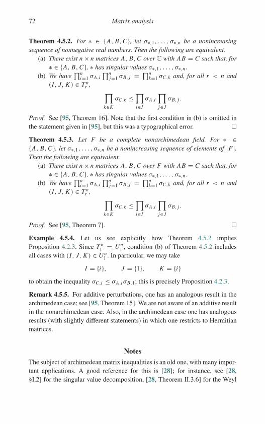
72 Matrix analysis
Theorem 4.5.2. For ∗ ∈ {A, B,C}, let σ∗,1, . . . , σ∗,n be a nonincreasingsequence of nonnegative real numbers. Then the following are equivalent.
(a) There exist n × n matrices A, B,C over C with AB = C such that, for∗ ∈ {A, B,C}, ∗ has singular values σ∗,1, . . . , σ∗,n.
(b) We have∏n
i=1 σA,i∏n
j=1 σB, j = ∏nk=1 σC,k and, for all r < n and
(I, J, K ) ∈ T nr , ∏
k∈K
σC,k ≤∏i∈I
σA,i
∏j∈J
σB, j .
Proof. See [95, Theorem 16]. Note that the first condition in (b) is omitted inthe statement given in [95], but this was a typographical error.
Theorem 4.5.3. Let F be a complete nonarchimedean field. For ∗ ∈{A, B,C}, let σ∗,1, . . . , σ∗,n be a nonincreasing sequence of elements of |F |.Then the following are equivalent.
(a) There exist n × n matrices A, B,C over F with AB = C such that, for∗ ∈ {A, B,C}, ∗ has singular values σ∗,1, . . . , σ∗,n.
(b) We have∏n
i=1 σA,i∏n
j=1 σB, j = ∏nk=1 σC,k and, for all r < n and
(I, J, K ) ∈ T nr , ∏
k∈K
σC,k ≤∏i∈I
σA,i
∏j∈J
σB, j .
Proof. See [95, Theorem 7].
Example 4.5.4. Let us see explicitly how Theorem 4.5.2 impliesProposition 4.2.3. Since T n
1 = U n1 , condition (b) of Theorem 4.5.2 includes
all cases with (I, J, K ) ∈ U n1 . In particular, we may take
I = {i}, J = {1}, K = {i}to obtain the inequality σC,i ≤ σA,iσB,1; this is precisely Proposition 4.2.3.
Remark 4.5.5. For additive perturbations, one has an analogous result in thearchimedean case; see [95, Theorem 15]. We are not aware of an additive resultin the nonarchimedean case. Also, in the archimedean case one has analogousresults (with slightly different statements) in which one restricts to Hermitianmatrices.
Notes
The subject of archimedean matrix inequalities is an old one, with many impor-tant applications. A good reference for this is [28]; for instance, see [28,§I.2] for the singular value decomposition, [28, Theorem II.3.6] for the Weyl
Notes 73
inequalities, in a much stronger form known as Weyl’s majorant theorem, [28,Theorem III.4.5] for a strong form of Proposition 4.2.3 (also a consequence ofthe Horn inequalities), and so on. (A variant of our Theorem 4.2.2 appears as[28, Problem I.6.11].)
The strong analogy between archimedean and p-adic matrix inequalitiesappears to be a little-known piece of folklore. As a result, we have been unableto locate a suitable reference.
It should be pointed out that most of what we have done here is the specialcase for GLn of a more general theory encompassing the other reductive alge-braic groups. This point of view can be seen in [95], where GLn makes someexplicit appearances for which other groups can be substituted.
In Theorem 4.1.13, the equivalence of (a) and (b) is standard. We do nothave a reference for the equivalence with (c), although it is implicit in mostproofs of the equivalence of (a) and (b).
The reader familiar with the notions of elementary divisors or invariant fac-tors may be wondering why the terminology “Hodge polygon” is necessaryor reasonable. The answer is that the Hodge numbers of a variety over a p-adic field are reflected by the elementary divisors of the action of Frobeniusgroups on crystalline cohomology. The fact that the Newton polygon liesabove the Hodge polygon then implies a relation between the characteristicpolynomial of Frobenius and the Hodge numbers of the original variety; thisrelationship was originally conjectured by Katz and proved by Mazur. See[27] for further discussion of this point and of crystalline cohomology as awhole.
Much of the work in this chapter can be carried over to the case of a transfor-mation which is only semilinear for some isometric endomorphism of F . Wewill adopt that point of view in Chapter 14; for instance, this will lead to a gen-eralization (in Theorem 14.5.5) of the Hodge–Newton decomposition theorem(Theorem 4.3.11). In this case, the carrying over is really in the other direc-tion: it is the latter result (due to Katz; see the notes for Chapter 14) whichinspired our presentation of Theorem 4.3.11 and its archimedean analogue(Theorem 4.1.12). Similarly, our treatment of Proposition 4.4.10 and its archi-medean analogue (Proposition 4.2.4) are modeled on [120, Corollary 1.4.4].
The question of quantifying the sensitivity to perturbation of the charac-teristic polynomial of a square matrix arises in numerical applications. Thequestion is familiar in the archimedean case but perhaps less so in the non-archimedean case; numerical applications of the latter include using p-adiccohomology to compute zeta functions of varieties over finite fields. See forinstance [3, §1.6] and [96, §3].
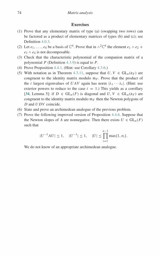
74 Matrix analysis
Exercises
(1) Prove that any elementary matrix of type (a) (swapping two rows) canbe factored as a product of elementary matrices of types (b) and (c); seeDefinition 4.0.3.
(2) Let e1, . . . , e4 be a basis of C4. Prove that in ∧2C4 the element e1 ∧ e2 +e3 ∧ e4 is not decomposable.
(3) Check that the characteristic polynomial of the companion matrix of apolynomial P (Definition 4.3.9) is equal to P .
(4) Prove Proposition 4.4.1. (Hint: use Corollary 4.3.6.)(5) With notation as in Theorem 4.3.11, suppose that U, V ∈ GLn(oF ) are
congruent to the identity matrix modulo mF . Prove that the product ofthe i largest eigenvalues of U AV again has norm |λ1 · · · λi |. (Hint: useexterior powers to reduce to the case i = 1.) This yields as a corollary[34, Lemma 5]: if D ∈ GLn(F) is diagonal and U, V ∈ GLn(oF ) arecongruent to the identity matrix modulo mF then the Newton polygons ofD and U DV coincide.
(6) State and prove an archimedean analogue of the previous problem.(7) Prove the following improved version of Proposition 4.4.6. Suppose that
the Newton slopes of A are nonnegative. Then there exists U ∈ GLn(F)such that
|U−1 AU | ≤ 1, |U−1| ≤ 1, |U | ≤n−1∏i=1
max{1, σi }.
We do not know of an appropriate archimedean analogue.
Part II
Differential Algebra

5
Formalism of differential algebra
In this chapter, we introduce some basic formalism of differential algebra.This may be viewed as a mild perturbation of commutative algebra in whichwe consider commutative rings equipped with the additional noncommutativestructure of a derivation. This allows us to manipulate differential equationsand differential systems in a manner that keeps the more useful structure visi-ble, though we will need to convert back and forth from this point of view. (Onething we will not do is generalize further, to the realm of differential schemesand sheaves; we leave this as a thought exercise for the curious reader.)
A particularly important result that we introduce is the cyclic vector theorem,which gives a compact but highly noncanonical way to represent a finite dif-ferential module over a field. While the cyclic vector theorem will proveindispensable at a few key points in our treatment of p-adic differentialequations, we will ultimately make more progress by limiting its use. SeeRemark 5.7.1 for further discussion.
5.1 Differential rings and differential modules
Definition 5.1.1. A differential ring is a commutative ring R equipped with aderivation d : R → R; the latter is an additive map satisfying the Leibniz rule
d(ab) = ad(b)+ bd(a) (a, b ∈ R).
We expressly allow d = 0 unless otherwise specified; this will be useful insome situations. A differential ring which is also a domain or field, etc., willbe called a differential domain, field, etc. Note that there is a unique extensionof d to any localization of R, using the quotient rule; in particular, if R is adomain then there is a unique extension of d to Frac(R).
77
78 Formalism of differential algebra
Definition 5.1.2. A differential module over a differential ring (R, d) is amodule M equipped with an additive map D : M → M satisfying
D(am) = aD(m)+ d(a)m;such a D will also be called a differential operator on M relative to d. Forexample, (R, d) is a differential module over itself; any differential moduleisomorphic to a direct sum of copies of (R, d) is said to be trivial. (If werefer to “the trivial differential module”, though, we mean (R, d) itself.) Adifferential module which is a successive extension of trivial modules is saidto be unipotent (see Proposition 7.2.5 for the reason why). A differential idealof R is a differential submodule of R itself, i.e., an ideal stable under d.
Definition 5.1.3. For (M, D) a differential module, define
H0(M) = ker(D), H1(M) = coker(D) = M/D(M).
The latter computes Yoneda extensions; see Lemma 5.3.3 below. Elements ofH0(M) are said to be horizontal (see the notes). Note that H0(R) = ker(d)is a subring of R; if R is a field then ker(d) is a subfield. We call them theconstant subring and constant subfield of R.
We now make an observation about base changes of the constant subring.For the definition of a more general base change, see Definition 5.3.2. (Seealso Proposition 6.9.1.)
Lemma 5.1.4. Let R0 be the constant subring of the differential ring (R, d),and let R′
0 be an R0-algebra. Let (M, D) be a differential module over (R, d).View R′ = R ⊗R0 R′
0 as a differential ring by defining the derivation d ′ by
d ′(∑
i
ai ⊗ ri
)=∑
i
d(ai )⊗ ri (ai ∈ R, ri ∈ R′0).
Similarly, view M ′ = M ⊗R0 R′0 as a differential module over (R′, d ′) by
defining the differential operator
D′(∑
i
mi ⊗ ri
)=∑
i
D(mi )⊗ ri (mi ∈ M, ri ∈ R′0).
(a) There are natural maps Hi (M)⊗R0 R′0 → Hi (M ′) for i = 0, 1.
(b) The map in (a) is always an isomorphism for i = 1.(c) If R′
0 is flat over R0 then the map in (a) is an isomorphism for i = 0.
5.1 Differential rings and differential modules 79
Proof(a) Tensoring the structure morphism R0 → R′
0 with M induces a mapM → M ′. This in turn induces maps Hi (M) → Hi (M ′) of R0-modules; using the R′-module structure on Hi (M ′), we also obtainmaps Hi (M)⊗R0 R′
0 → Hi (M ′).(b) Tensoring with R′
0 is always a right exact functor on R0-modules.Since
MD→ M → H1(M)→ 0
is an exact sequence in the category of R0-modules,
M ′ D′→ M ′ → H1(M)⊗R0 R′0 → 0
is also exact. Hence the induced map H1(M)⊗R0 R′0 → H1(M ′) is an
isomorphism.(c) Recall that, by definition, R′
0 is flat over R0 if and only if tensoring withR′
0 is an exact functor on R0-modules. Since
0 → H0(M)→ MD→ M
is an exact sequence in the category of R0-modules,
0 → H0(M)⊗R0 R′0 → M ′ D′→ M ′
is also exact. Hence the induced map H0(M)⊗R0 R′0 → H0(M ′) is an
isomorphism.
Another frequently used observation is the following.
Lemma 5.1.5. Let (R, d) be a differential field with constant subfield R0.Then, for any differential module (M, D) over (R, d), the natural mapH 0(M)⊗R0 R → M is injective. In particular, dimR0 H0(M) ≤ dimR M.
Proof. An equivalent statement is that if m1, . . . ,mn ∈ H0(M) are linearlydependent over R then they are also linearly dependent over R0. Suppose onthe contrary that, for some positive integer n, there exist m1, . . . ,mn ∈ H0(M)which are linearly dependent over R but linearly independent over R0. Choosen as small as possible with this property; then there exist c1, . . . , cn ∈ R allnonzero such that c1m1+· · ·+cnmn = 0. We may rescale the ci so that c1 = 1.
Since m1, . . . ,mn ∈ H0(M), we also have
d(c1)m1 + · · · + d(cn)mn = 0.
80 Formalism of differential algebra
That is, d(c1), . . . , d(cn) form another linear dependence relation betweenm1, . . . ,mn . But d(c1) = d(1) = 0, so to avoid contradicting the choice ofn we must have d(c2) = · · · = d(cn) = 0. That is, c1, . . . , cn ∈ R0, contra-dicting the hypothesis that m1, . . . ,mn are linearly independent over R0. Thiscontradiction proves the claim.
Definition 5.1.6. Let M be a differential module over a differential ring Radmitting a finite exhaustive filtration with irreducible successive quotients.(For instance, R could be a differential field and M could be a finitely gen-erated differential module over R.) Then the multiset of these quotients isindependent of the choice of the filtration; we call them the (Jordan–Hölder)constituents of M .
5.2 Differential modules and differential systems
We now describe the link between differential modules and linear differentialsystems.
Definition 5.2.1. Let R be a differential ring, and let M be a finite free differ-ential module of rank n over R. Let e1, . . . , en be a basis of M . Then, for anyv ∈ M , we can write v = v1e1 + · · · + vnen for some v1, . . . , vn ∈ R andcompute
D(v) = v1 D(e1)+ · · · + vn D(en)+ d(v1)e1 + · · · + d(vn)en .
Define the matrix of action of D (i.e., the matrix representing the action of D)on the basis e1, . . . , en to be the n × n matrix N over R given by the formula
D(e j ) =n∑
i=1
Ni j ei .
We then have
D(v) =n∑
i=1
⎛⎝d(vi )+n∑
j=1
Ni jv j
⎞⎠ ei .
That is, if we identify v with the column vector [v1 · · · vn] then
D(v) = Nv + d(v).
Conversely, it is clear that, given the underlying finite free R-module, anydifferential module structure is given by such an equation.
5.3 Operations on differential modules 81
Definition 5.2.2. With notation as in Definition 5.2.1, let v1, . . . , vn be a sec-ond basis of M . The change-of-basis matrix from e1, . . . , en to v1, . . . , vn isthe n × n matrix U defined by
v j =∑
i
Ui j ei .
The effect of changing basis is that the matrix of action of D on v1, . . . , vn is
U−1 NU + U−1d(U ).
Remark 5.2.3. In other words, differential modules are a coordinate-free ver-sion of differential systems. If you are a geometer, you may wish to go furtherand think of differential bundles, i.e., vector bundles equipped with a differ-ential operator. A differential operator on a vector bundle is usually called aconnection.
5.3 Operations on differential modules
We now describe the basic operations in the category of differential modulesover a differential ring.
Definition 5.3.1. For R a differential ring, we regard the differential modulesover R as a category in which the morphisms (or homomorphisms) from M1
to M2 are R-module homomorphisms f : M1 → M2 satisfying D( f (m)) =f (D(m)) (we sometimes say these maps are horizontal).
Definition 5.3.2. The category of differential modules over a differential ringadmits certain functors corresponding to familiar functors on the category ofmodules over an ordinary ring, such as the following. (Be aware that in thefollowing notation the subscripted R on such symbols as the tensor productwill often be suppressed when it is unambiguous. Our habit tends to be todrop the subscript when tensoring modules over a single ring but not whenperforming a base change.)
Given two differential modules M1,M2, the tensor product M1 ⊗R M2
in the category of rings may be viewed as a differential module via theformula
D(m1 ⊗ m2) = D(m1)⊗ m2 + m1 ⊗ D(m2).
This in particular gives meaning to the base change M ⊗R R′ of a differentialR-module M to a differential R-algebra R′; we also denote this by f ∗M if f
82 Formalism of differential algebra
is the map from R to R′. Similarly, the exterior power ∧nR M may be viewed as
a differential module via the formula
D(m1 ∧ · · · ∧ mn) =n∑
i=1
m1 ∧ · · · ∧ mi−1 ∧ D(mi ) ∧ mi+1 ∧ · · · ∧ mn .
(A similar fact is true for the symmetric power SymnR M , but we will have
no need of this.) The module of R-homomorphisms HomR(M1,M2) may beviewed as a differential module via the formula
D( f )(m) = D( f (m))− f (D(m));the homomorphisms from M1 to M2 as differential modules are precisely thehorizontal elements of HomR(M1,M2). (In this case, the subscript is quitecrucial: we have Hom(M1,M2) = H0(HomR(M1,M2)).)
We write M∨1 for HomR(M1, R) and call it the dual of M1; if M1 is finite
free then HomR(M1,M2) ∼= M∨1 ⊗ M2 and the natural map M1 → (M∨
1 )∨
is an isomorphism. In particular, M∨1 ⊗ M1 contains a horizontal element cor-
responding to the identity map M1 → M1; we call this the trace (element) ofM∨
1 ⊗M1, and we call the trivial submodule generated by the trace element thetrace component of M∨
1 ⊗ M1. If R is a Q-algebra then M∨1 ⊗ M1 splits as the
direct sum of the trace component with the set of elements of HomR(M1,M2)
of trace zero; we call the latter the trace-zero component of M∨1 ⊗ M1. Even
if R is not a Q-algebra, we can still view the trace component as a quotient ofM∨
1 ⊗ M1 by duality, but the map given by embedding the trace componentinto M∨
1 ⊗ M1 and then projecting onto the trace component need not be anisomorphism.
Lemma 5.3.3. Let M, N be differential modules with M finite free. Then thegroup H1(M∨ ⊗ N ) is canonically isomorphic to the Yoneda extension groupExt(M, N ).
Proof. The group Ext(M, N ) consists of equivalence classes of exact seq-uences 0 → N → P → M → 0 under the relation that this sequenceis equivalent to a second sequence 0 → N → P ′ → M → 0 if thereis an isomorphism P ∼= P ′ that induces the identity maps on M and N .Addition consists of taking two such sequences and returning the Baer sum0 → N → Q/�→ M → 0, where Q is the set of elements in P ⊕ P ′ whoseimages in M coincide and � = {(n,−n) ∈ Q : n ∈ N }. The identity elementis the split sequence 0 → N → M ⊕ N → M → 0. The inverse of a sequence0 → N → P → M → 0 is the same sequence with the map N → P negated.(See [216, §3.4] for the proof that this indeed gives a group.)

5.3 Operations on differential modules 83
We first construct a canonical isomorphism Ext(M, N )→ Ext(R,M∨⊗N ).Given an extension 0 → N → P → M → 0, tensor with M∨ to get
0 → M∨ ⊗ N → M∨ ⊗ P → M∨ ⊗ M → 0.
Let Q be the inverse image of the trace component of M∨ ⊗ M ; we then getan extension
0 → M∨ ⊗ N → Q → R → 0,
yielding a map Ext(M, N ) → Ext(R,M∨ ⊗ N ), which is easily shown to bea homomorphism. In the other direction, given an extension
0 → M∨ ⊗ N → Q → R → 0,
tensor with M to get
0 → M ⊗ M∨ ⊗ N → M ⊗ Q → M → 0,
then quotient M ⊗ Q by the kernel of the projection M ⊗ M∨ → R tensoredwith N . These are seen to be inverses by a diagram-chasing argument, whichwe omit.
By the previous paragraph, we may reduce the statement of the lemmato the case M = R. (One can also describe the construction without firstmaking this reduction, but it is a bit harder to follow.) Given an extension0 → N → P → R → 0, compute H 0 and H1 and apply the snake lemma toobtain a connecting homomorphism H0(R) → H 1(N ). The image of 1 ∈ Runder this homomorphism determines an element of H1(N ), thus giving amap Ext(R, N ) → H1(N ). This map is easily shown to be a homomorphism(exercise).
It remains to construct an inverse map. Given an element of H1(N ) repre-sented by x ∈ N , we equip N ⊕ R with the structure of a differential moduleby setting
D(n, r) = (D(n)+ r x, d(r)).
This module is indeed an extension of the desired form, and the image of 1 ∈ Runder the resulting connecting homomorphism is precisely the class of x inH 1(N ). In the other direction, any extension splits at the level of modules andso must have this form for some x ∈ N . This yields the claim.
Remark 5.3.4. Although we will not need this, we note that the isomor-phisms HomR(M1,M2) ∼= M∨
1 ⊗ M2 and M1 → (M∨1 )
∨, and the assertionof Lemma 5.3.3, also carry over to the case where M1 is a finite projectiveR-module, i.e., a direct summand of a finite free R-module. Such a module is
84 Formalism of differential algebra
always flat. If R is noetherian then a finitely generated R-module M is projec-tive if and only if it is locally free, i.e., if there exists a finite subset f1, . . . , fm
of R, generating the unit ideal, such that M[ f −1i ] is free over R[ f −1
i ] for eachi [84, Exercise 4.12].
5.4 Cyclic vectors
Definition 5.4.1. Let R be a differential ring, and let M be a finite free differ-ential module of rank n over R. A cyclic vector for M is an element m ∈ Msuch that m, D(m), . . . , Dn−1(m) form a basis of M .
Theorem 5.4.2 (Cyclic vector theorem). Let R be a differential field of char-acteristic 0 with nonzero derivation. Then every finite differential module overR has a cyclic vector.
Many proofs are possible; we give here the proof from [80, TheoremIII.4.2]. For another proof that applies over some rings other than fields, seeTheorem 5.7.3 below. See also the notes for further discussion. (For a commenton characteristic p, see the exercises.)
Proof. We start by normalizing the derivation. For u ∈ R×, given one differen-tial module (M, D) over (R, d), we get another differential module (M, u D)over (R, ud), and m is a cyclic vector for one of these modules if and only if itis a cyclic vector for the other (because the image of m under (u D) j is in thespan of m, D(m), . . . , D j (m)). We may thus assume (thanks to the assump-tion that the derivation is nontrivial) that there exists a nonzero element x ∈ Rsuch that d(x) = x .
Let M be a differential module of dimension n, and choose m ∈ M suchthat the dimension μ of the span of m, D(m), . . . is as large as possible. Wederive a contradiction under the hypothesis μ < n.
For z ∈ M and λ ∈ Q, we have
(m + λz) ∧ D(m + λz) ∧ · · · ∧ Dμ(m + λz) = 0
in the exterior power ∧μ+1 M . If we write this expression as a polyno-mial in λ, it vanishes for infinitely many values so must be identically zero.Hence each coefficient must vanish separately, including the coefficient of λ1,which is
μ∑i=0
m ∧ · · · ∧ Di−1(m) ∧ Di (z) ∧ Di+1(m) ∧ · · · ∧ Dμ(m). (5.4.2.1)
5.5 Differential polynomials 85
Pick s ∈ Z, substitute xs z for z in (5.4.2.1), divide by xs , and set the resultequal to zero. We get
μ∑i=0
si�i (m, z) = 0 (s ∈ Z) (5.4.2.2)
for
�i (m, z)=μ−i∑j=0
(i+ j
i
)m∧· · ·∧Di+ j−1(m)∧D j (z)∧Di+ j+1(m)∧· · ·∧Dμ(m).
Again because we are in characteristic zero, we may conclude that (5.4.2.2),viewed as a polynomial in s, has all coefficients equal to zero; that is,�i (m, z) = 0 for all m, z ∈ M .
We now take i = μ to obtain
(m ∧ · · · ∧ Dμ−1(m)) ∧ z = 0 (m, z ∈ M);since μ < n, we may use this to deduce that
m ∧ · · · ∧ Dμ−1(m) = 0 (m ∈ M).
But this means that the dimension of the span of m, D(m), . . . is at most μ−1,contradicting the definition of μ.
5.5 Differential polynomials
We now give the interpretation of differential modules as modules over amildly noncommutative ring.
Definition 5.5.1. Let (R, d) be a differential ring. The ring of twistedpolynomials R{T } over R in the variable T is the additive group
R ⊕ (R · T )⊕ (R · T 2)⊕ · · · ,with noncommuting multiplication given by the formula( ∞∑
i=0
ai Ti
)⎛⎝ ∞∑j=0
b j Tj
⎞⎠ =∞∑
i, j=0
j∑h=0
(j
h
)ai d
h(b j )Ti+ j−h .
In other words, we impose the relation
T a = aT + d(a) (a ∈ R)
and then check that the result is a not necessarily commutative ring (see theexercises). We define the degree of a twisted polynomial, in the usual way,
86 Formalism of differential algebra
as the exponent of the largest power of T with a nonzero coefficient; thedegree of the zero polynomial may be taken to be any particular negativevalue.
Proposition 5.5.2 (Ore). For R a differential field, the ring R{T } admits a leftdivision algorithm. That is, if f, g ∈ R{T } and g �= 0 then there exist uniqueq, r ∈ R{T } with deg(r) < deg(g) and f = gq + r . (There is also a rightdivision algorithm.)
Proof. Exercise.
Using the Euclidean algorithm, this yields the following consequence as inthe untwisted case.
Theorem 5.5.3 (Ore). Let R be a differential field. Then R{T } is both leftprincipal and right principal; that is, any left ideal (resp. right ideal) has theform R{T } f (resp. f R{T }) for some f ∈ R{T }.Definition 5.5.4. Note that the ring opposite to R{T }, i.e., the ring in whichmultiplication is performed by first switching the order of the factors, is againa twisted polynomial ring except that the derivation is −d instead of d. Givenf ∈ R{T }, we define the formal adjoint of f as the element f in the oppositering. This operation looks a bit less formal if we also take the coefficients overto the other side, giving what we will call the adjoint form of f . For instance,the adjoint form of T 3 + aT 2 + bT + c is
T 3 + T 2a + T (b − 2d(a))+ d2(a)− d(b)+ c.
Remark 5.5.5. The twisted polynomial ring is engineered precisely so that, forany differential module M over R, we obtain an action of R{T } on M underwhich T acts like D. In particular, R{T } acts on R itself with T acting like d.In fact, the category of differential modules over R is equivalent to the categoryof left R{T }-modules. Moreover, if M is a finite differential module over R,any cyclic vector m ∈ M corresponds to an isomorphism M ∼= R{T }/R{T }Pfor some monic twisted polynomial P , where the isomorphism carries m tothe class of 1. (We can think of f as a sort of “characteristic polynomial” forM , except that it depends strongly on the choice of the cyclic vector.) Undersuch an isomorphism, a factorization P = P1 P2 corresponds to a short exactsequence 0 → M1 → M → M2 → 0 with
M1 ∼= R{T }P2/R{T }P ∼= R{T }/R{T }P1, M2 ∼= R{T }/R{T }P2.
5.7 Cyclic vectors: a mixed blessing 87
5.6 Differential equations
You may have been wondering when differential equations will appear, as thesepurport to be the objects of study of this book. If so, your wait is over.
Definition 5.6.1. A differential equation of order n over the differential ring(R, d) is an equation of the form
(andn + · · · + a1d + a0)y = b,
with a0, . . . , an, b ∈ R, and y indeterminate. We say the equation is homo-geneous if b = 0 and inhomogeneous otherwise.
Remark 5.6.2. Using our setup, we may write this equation as f (d)y = bfor some f ∈ R{T }. Similarly, we may view systems of differential equationsas being equations of the form f (D)y = b, where b lives in some differentialmodule (M, D). By the usual method (i.e. introducing extra variables corre-sponding to derivatives of y), we can convert any differential system into afirst-order system Dy = b. We can also convert an inhomogeneous systeminto a homogeneous one by adding an extra variable, with the understandingthat we would like the value of that last variable to be 1 in order to get back asolution of the original equation.
Remark 5.6.3. Here is a more explicit relationship between adjoint polyno-mials and the process of solving differential equations. Suppose that you startwith the cyclic differential module M ∼= R{T }/R{T } f and you want to finda horizontal element. That means that you want to find some g ∈ R{T } suchthat T g ∈ R{T } f ; we may as well assume that deg(g) < deg( f ). Then, bycomparing degrees, we see that in fact T g = r f for some r ∈ R. Write f inadjoint form as f0 + T f1 + · · · + T n ; then
r f ≡ r f0 − d(r) f1 + d2(r) f2 − · · · + (−1)ndn(r) (mod T R{T }).In this manner, finding a horizontal element becomes equivalent to solving adifferential equation.
5.7 Cyclic vectors: a mixed blessing
The reader may at this point be wondering why so many points of view arenecessary, since the cyclic vector theorem can be used to transform any differ-ential module into a differential equation, and ultimately differential equationsare the things one writes down and wants to solve. Permit me to interject herea countervailing opinion.
88 Formalism of differential algebra
Remark 5.7.1. In ordinary linear algebra (or in other words, when consider-ing differential modules for the trivial derivation), one can pass freely betweenlinear transformations on a vector space and square matrices if one is willing tochoose a basis. The merits of doing this depend on the situation, so it is valu-able to have both the matricial and coordinate-free viewpoints well in hand.One can then pass to the characteristic polynomial, but not all information isretained (one loses information about nilpotency) and even information thatin principle is retained is sometimes not so conveniently accessed. In short,no one would seriously argue that one can dispense with studying matricesbecause of the existence of the characteristic polynomial.
The situation is not so different in the differential case. The differencebetween a differential module and a differential system is merely the choice ofa basis, and again it is valuable to have both points of view in mind. However,the cyclic vector theorem may seduce one into thinking that collapsing a differ-ential system into a differential polynomial is an operation without drawbacks,but this is far from the case. For instance, determining whether two differentialpolynomials correspond to the same differential system is not straightforward.
More seriously for our purposes, the cyclic vector theorem only appliesover a differential field. Many differential modules are more naturally definedover some ring which is not a field. For instance, differential modules aris-ing from geometry (such as Picard–Fuchs modules) are usually defined overa ring of functions on some geometric space. While there are forms of thecyclic vector theorem available over nonfields (see for instance Theorem 5.7.3below), these do not suffice for our purposes. We also find that working withdifferential modules instead of differential polynomials has a tremendouslyclarifying effect, partly because it improves the parallelism with differencealgebra, where there is no good analogue of the cyclic vector theorem evenover a field. (See Part IV.)
We find it unfortunate that much literature on complex ordinary differ-ential equations, and nearly all the literature on p-adic ordinary differentialequations, is mired in the language of differential polynomials. By switchinginstead between differential modules and differential polynomials, as appro-priate, we will be able to demonstrate strategies that lead to a more systematicdevelopment of p-adic theory.
As promised, we offer some results concerning cyclic vectors over rings,due to Katz [122].
Theorem 5.7.2. Let R be a differential local Q-algebra. Suppose that the max-imal ideal of R contains an element t such that d(t) = 1. Let M be a finite freedifferential module over R, and let e1, . . . , en be a basis of M. Then
5.7 Cyclic vectors: a mixed blessing 89
v =n−1∑j=0
t j
j !j∑
k=0
(−1)k(
j
k
)Dk(e j+1−k)
is a cyclic vector of M.
Proof. For i, j ≥ 0, put
c(i, j) =j∑
k=0
(−1)k(
j
k
)Dk(ei+ j+1−k)
with the convention that eh = 0 for h > n. It is easily checked that
c(i + 1, j) = D(c(i, j))+ c(i, j + 1).
By induction on i , we find that
Di (v) =n−1∑j=0
t j
j !c(i, j) ≡ ei+1 (mod t).
Hence v, D(v), . . . , Dn−1(v) freely generate M modulo the maximal idealof R. They thus freely generate M itself by Nakayama’s lemma [84,Corollary 4.8].
Theorem 5.7.3. Let R be a differential Q-algebra containing an element t forwhich d(t) = 1. Let M be a finite free differential module over R, and let Ibe a prime ideal of R. Then there exists f ∈ R \ I such that M ⊗R R[ f −1]contains a cyclic vector.
Proof. Choose a basis e1, . . . , en of M , and define c(i, j) as in the proof ofTheorem 5.7.2. For x ∈ R, put
ci (x) =n−1∑j=0
x j
j ! c(i, j).
Then there exists a polynomial P(T ) ∈ R[T ] such that
c0(x) ∧ · · · ∧ cn−1(x) = P(x)(e1 ∧ · · · ∧ en) (x ∈ R).
Since c(i, 0) = ei+1, we have P(0) = 1. In particular, the image Q(T ) ∈(R/I )[T ] of P(T ) is not identically zero.
Since R contains Q, the images of t − a for a ∈ Z are all distinct, so onlyfinitely many of them are roots of Q(T ). We can thus choose a ∈ Z such thatP(t − a) /∈ I . Since
Di (c0(t − a)) = ci (t − a)
90 Formalism of differential algebra
as in the previous proof, c0(t − a) is a cyclic vector of M ⊗R R[ f −1] forf = P(t − a), as desired.
5.8 Taylor series
Definition 5.8.1. Let R be a topological differential ring, i.e., a ring equippedwith a topology and a derivation such that all operations are continuous.Assume also that R is a Q-algebra. Let M be a topological differential moduleover R, i.e., a differential module such that all operations are continuous. Forr ∈ R and m ∈ M , we define the Taylor series T (r,m) as the infinite sum
∞∑i=0
r i
i ! Di (m)
whenever the sum converges absolutely (i.e., all rearrangements converge tothe same value).
Remark 5.8.2. The expression T (r,m) is de facto additive in m: ifm1,m2 ∈ M then
T (r,m1)+ T (r,m2) = T (r,m1 + m2)
whenever all three terms are well-defined. For s ∈ R, T (r, s) is also de factomultiplicative: if s1, s2 ∈ R, then (by the Leibniz rule)
T (r, s1)T (r, s2) = T (r, s1s2)
whenever all three terms are well-defined. More generally, for m ∈ M , T (r,m)is de facto semilinear: if s ∈ R, m ∈ M then
T (r, s)T (r,m) = T (r, sm)
whenever all three terms are well-defined.
Example 5.8.3. A key instance of the previous remark is the case where R isa completion of a rational function field F(t) and d is the differential operatord/dt . In this case, the ring homomorphism T (r, ·) is the substitution t �→ t+r ;note that this makes sense only if |r | ≤ 1.
Remark 5.8.4. Another use for Taylor series is to construct horizontalsections. Note that
D(T (r,m)) =∞∑
i=1
d(r)r i−1
(i − 1)! Di (m)+∞∑
i=0
r i
i ! Di+1(m)
= (1 + d(r))T (r,m)
Exercises 91
if everything converges absolutely. In particular, if d(r) = −1 then T (r,m) ishorizontal.
Notes
The subject of differential algebra is rather well developed; a classic treatment,though possibly too dry to be useful to the casual reader, is the book of Ritt[188]. As in abstract algebra in general, the development of differential algebrawas partly driven by differential Galois theory, i.e., the study of the expressionof solutions of differential equations in terms of solutions to ostensibly simplerdifferential equations. A relatively lively introduction to the latter is [202].
Calling an element of a differential module horizontal when it is killed bythe derivation makes sense if you consider connections in differential geome-try. In that setting, the differential operator is measuring the extent to which asection of a vector bundle deviates from some prescribed “horizontal” directionidentifying points on one fibre with points on nearby fibres.
The history of the cyclic vector theorem is rather complicated. It appearsto have been first proved by Loewy [162] in the case of meromorphic func-tions, and (independently) by Cope [60] in the case of rational functions. For adetailed historical discussion, see [53].
Twisted polynomials were introduced by Ore [177]. They are actually some-what more general than we have discussed; for instance, one can also twistby an endomorphism τ : R → R by imposing the relation T a = τ(a)T .(This enters the realm of the analogue of differential algebra called differencealgebra, which we will treat in Part IV.) Moreover, one can twist by both anendomorphism and a derivation if they are compatible in an appropriate way,and one can even study differential or difference Galois theory in this set-ting. A unifying framework for doing so, which is also suitable for consideringmultiple derivations and automorphisms, was given by André [4].
Differential algebra in positive characteristic has a rather different flavorthan in characteristic 0; for instance, the pth power of the derivation d/dt onFp(t) is the zero map. A brief discussion of the characteristic-p situation isgiven in [80, §III.1].
Exercises
(1) Prove that if M is a locally free differential module over R of rank 1 thenM∨ ⊗ M is trivial (as a differential module).
(2) Check that the bijection Ext(R, N ) → H1(N ) constructed in the proof ofLemma 5.3.3 is indeed a homomorphism.
92 Formalism of differential algebra
(3) Check that, in characteristic p > 0, the cyclic vector theorem holds formodules of rank at most p but may fail for modules of rank p + 1.
(4) Give a counterexample to the cyclic vector theorem for a differential fieldof characteristic 0 with trivial derivation.
(5) Verify that R{T } is indeed a not necessarily commutative ring; the contentin this exercise is to check the associativity of multiplication.
(6) Prove the division algorithm (Proposition 5.5.2).
6
Metric properties of differential modules
In this chapter, we study the metric properties of differential modules over non-archimedean differential rings. The principal invariant that we will identify isa familiar quantity from functional analysis known as the spectral radius of abounded endomorphism. When applied to the derivation acting on a differen-tial module, we obtain a quantity which can be related to the least slope of theNewton polygon of the corresponding twisted polynomial.
We can give meaning to the other slopes as well, by proving that over acomplete nonarchimedean differential field any differential module decom-poses into components whose spectral radii are computed by the variousslopes of the Newton polygon. However, this theorem will provide some-what incomplete results when we apply it to p-adic differential modules inPart III; we will have to remedy the situation using Frobenius descendants andantecedents.
This chapter provides important foundational material for much of whatfollows, but on its own it may prove indigestably abstract at first. The readerarriving at this opinion is advised to read Chapter 7 in conjunction with thisone, to see how the constructions of this chapter become explicit in a simplebut important class of examples.
6.1 Spectral radii of bounded endomorphisms
Before considering differential operators, let us recall the difference betweenthe operator norm and the spectral radius of a bounded endomorphism of anabelian group.
Hypothesis 6.1.1. Throughout this section, let G be a nonzero abelian groupequipped with a norm | · |, and let T : G → G be a bounded endomorphism
93
94 Metric properties of differential modules
of G. Recall that this means that there exists c ≥ 0 such that |T (g)| ≤ c|g| forall g ∈ G.
Definition 6.1.2. The operator norm |T |G of T is defined to be the least c ≥ 0for which |T (g)| ≤ c|g| for all g ∈ G, i.e.,
|T |G = supg∈G,g �=0
{|T (g)|/|g|}.
Recall that, if M is a finite free module over a nonarchimedean ring R, | · |M isthe supremum norm for some basis, and T is an R-linear transformation, then|T | = |A|, where A is the matrix of action of T on the chosen basis of M and|A| = supi j {|Ai j |} as in Chapter 4.
One can similarly define the operator norm for a map between two differentabelian groups, each equipped with a norm. We may even allow seminorms aslong as we take the supremum over elements of the source group which are notin the kernel of the seminorm.
Although the condition that T is bounded is preserved on replacing the normby a metrically equivalent norm, the operator norm is not preserved. To obtaina less fragile numerical invariant, we introduce the spectral radius.
Definition 6.1.3. The spectral radius of T is defined as
|T |sp,G = lims→∞ |T s |1/sG ;
the existence of the limit follows from the fact |T m+n|G ≤ |T m |G |T n|G andfrom the following lemma.
Lemma 6.1.4 (Fekete). Let {an}∞n=1 be a sequence of real numbers such thatam+n ≥ am + an for all m, n. Then the sequence {an/n}∞n=1 either convergesto its supremum or diverges to +∞.
Proof. Exercise.
Proposition 6.1.5. The spectral radius of T depends on the norm | · | only upto metric equivalence.
Proof. Suppose that | · |′ is a norm metrically equivalent to | · |. We can thenchoose c > 0 such that c−1|g| ≤ |g|′ ≤ c|g| for all g ∈ G. We then have|T (g)|/|g| ≤ c2|T (g)|′/|g|′ for all g ∈ G \ {e}. Applying this with T replacedby T s gives |T s |G ≤ c2|T s |′G , so
|T s |sp,G ≤ lims→∞ c2/s(|T s |′sp,G)
1/s .
6.2 Spectral radii of differential operators 95
Since c2/s → 1 as s → ∞, this gives |T s |sp,G ≤ |T s |′sp,G . The reverseinequality is found to hold on reversing the roles of the norms.
We have the following relationship to the concepts studied in Chapter 4.
Remark 6.1.6. Let F be a field equipped with a norm, and let V be a finite-dimensional vector space over F . Pick a basis for V , and equip V with eitherthe L2 norm or the supremum norm defined by this basis, according to whetherF is archimedean or nonarchimedean. Let A be the matrix of action of T onthis basis. Then |T |V equals the largest singular value of A, whereas |T |sp,V
equals the largest norm of an eigenvalue of A (by Proposition 4.2.4 in thearchimedean case, and Proposition 4.4.10 in the nonarchimedean case).
Remark 6.1.7. The spectral radius derives its name from the fact that, by acelebrated theorem of Gelfand, for a bounded endomorphism of a commutativeBanach algebra over R or C the spectral radius computes the radius of thesmallest disc containing the entire spectrum of the operator. (This includes thearchimedean case of the previous remark.)
When dealing with the spectral radius we will frequently use the followingobservation.
Lemma 6.1.8. For any ε > 0 there exists c = c(ε) such that for all s ≥ 0,
|T s |G ≤ c(|T |sp,G + ε)s .
Proof. For c = 1, the claim already holds for all but finitely many s. It thussuffices to increase c in order to cover the finite set of exceptions.
Remark 6.1.9. Some authors writing about p-adic differential equations(including the present author) tend to refer to the spectral radius as the spec-tral norm. On the one hand, this is somewhat dangerous, because the spectralradius is not in general a norm or even a seminorm, even for matrices overa complete field (exercise). On the other hand, we will be using the spectralradius as a measure of size and so the normlike notation | · |sp,V is useful. Wewill compromise by keeping this notation but referring to spectral radii ratherthan spectral norms.
6.2 Spectral radii of differential operators
We now specialize the previous discussion to the case of differential modules.
Definition 6.2.1. By a nonarchimedean differential ring or field, we meana nonarchimedean ring equipped with a bounded derivation. For F a
96 Metric properties of differential modules
nonarchimedean differential field, we can define the operator norm |d|F andthe spectral radius |d|sp,F ; by hypothesis the former is finite, so the latter is too.
Definition 6.2.2. Let F be a nonarchimedean differential field. By a normeddifferential module over F we mean a vector space V over F equipped with acompatible norm | · |V and a derivation D with respect to d which is boundedas a endomorphism of the additive group of V . For V nonzero, we may thenconsider the operator norm |D|V and the spectral radius |D|sp,V .
Remark 6.2.3. If V is finite-dimensional over F and F is complete then thespectral radius does not depend on the norm on V , since by Theorem 1.3.6 anytwo norms on V compatible with the norm on F are metrically equivalent.
In general, one cannot have differential modules with arbitrarily smallspectral radius.
Lemma 6.2.4. Let F be a nonarchimedean differential field, and let V be anonzero normed differential module over F. Then
|D|sp,V ≥ |d|sp,F .
Proof. (This proof was suggested by Liang Xiao.) For a ∈ F and v ∈ Vnonzero, the Leibniz rule gives
Ds−i (aDi (v))= ds−i (a)Di (v)+s−i∑j=1
(s−i
j
)ds−i− j (a)Di+ j (v) (0 ≤ i ≤ s).
Inverting this system of equations gives an identity of the form
ds(a)v =s∑
i=0
cs,i Ds−i (aDi (v))
for certain universal constants cs,i ∈ Z. Consequently,
|ds(a)v|V ≤ max0≤i≤s
{|Ds−i (aDi (v))|V }. (6.2.4.1)
By Lemma 6.1.8, given ε > 0 we can choose c = c(ε) such that, for all s ≥ 0,
|Ds |V ≤ c(|D|sp,V + ε)s .
Using (6.2.4.1), we deduce that
|ds(a)v|V ≤ c2(|D|sp,V + ε)s |a||v|V .Dividing by |a||v|V and taking the supremum over a ∈ F , we obtain
|ds |F ≤ c2(|D|sp,V + ε)s .

6.2 Spectral radii of differential operators 97
Taking sth roots and then letting s → ∞, we get
|d|sp,F ≤ |D|sp,V + ε.
Since ε > 0 was arbitrary, this yields the claim.
It is sometimes useful to compute in terms of a basis of V over F .
Lemma 6.2.5. Let F be a complete nonarchimedean differential field, andlet V be a nonzero finite differential module over F. Fix a basis e1, . . . , en
of V , and let Ds be the matrix of action of Ds on this basis (i.e., Ds(e j ) =∑i (Ds)i j ei ). Then
|D|sp,V = max{|d|sp,F , lim sups→∞
|Ds |1/s}. (6.2.5.1)
Proof. (Compare [49, Proposition 1.3].) Equip V with the supremum normdefined by e1, . . . , en ; then |Ds |V ≥ maxi, j |(Ds)i, j |. This plus Lemma 6.2.4imply that the left-hand side of (6.2.5.1) is greater than or equal to the theright-hand side.
Conversely, for any x ∈ V , if we write x = x1e1 + · · · + xnen withx1, . . . , xn ∈ F then
Ds(x) =n∑
i=1
s∑j=0
(s
j
)d j (xi )D
s− j (ei ),
so
|Ds |1/sV ≤ max0≤ j≤s
{|d j |1/sF |Ds− j |1/s
}. (6.2.5.2)
Given ε > 0, apply Lemma 6.1.8 to choose c = c(ε) such that, for all s ≥ 0,
|ds |F ≤ c(|d|sp,F + ε
)s,
|Ds |V ≤ c
(lim sup
s→∞|Ds |1/s + ε
)s
.
Then (6.2.5.2) implies that
|Ds |1/sV ≤ c2/s max
{|d|sp,F + ε, lim sup
s→∞|Ds |1/s + ε
}.
As in the previous proof, the factor c2/s tends to 1 as s → ∞. From this itfollows that the right-hand side of (6.2.5.1) is greater than or equal to the left-hand side minus ε; since ε > 0 was arbitrary, we get the same inequality withε = 0.
Remark 6.2.6. In Lemma 6.2.5, if |D|sp,V > |d|sp,F then the limit superiorcan be replaced by a limit; see the exercises.
98 Metric properties of differential modules
Using Lemma 6.2.5, we may infer the following base-change property forthe spectral radius. We will need to refine this result later; see Corollary 6.5.5and Proposition 10.6.6 below.
Corollary 6.2.7. Let F → F ′ be an isometric embedding of complete nonar-chimedean differential fields. (In particular, the differential on F ′ must restrictto the differential on F.) Then, for any nonzero finite differential module Vover F,
|D|sp,V ′ = max{|d|sp,F ′ , |D|sp,V }.Consequently, if |d|sp,F ′ = |d|sp,F then |D|sp,V ′ = |D|sp,V by Lemma 6.2.4.
Proof. Choose a basis of V , and use Lemma 6.2.5 to compute both |D|sp,V
and |D|sp,V ′ in terms of this basis. This yields the desired formula.
Here is how the spectral radius behaves with respect to basic operations onthe category of differential modules.
Lemma 6.2.8. Let F be a complete nonarchimedean differential field.(a) For a short exact sequence 0 → V1 → V → V2 → 0 of nonzero finite
differential modules over F,
|D|sp,V = max{|D|sp,V1 , |D|sp,V2}.(b) For V a nonzero finite differential module over F,
|D|sp,V ∨ = |D|sp,V .
(c) For V1, V2 nonzero finite differential modules over F,
|D|sp,V1⊗V2 ≤ max{|D|sp,V1 , |D|sp,V2},with equality when |D|sp,V1 �= |D|sp,V2 .
Proof. To prove (a), choose a splitting V = V1⊕V2 of the short exact sequencein the category of vector spaces over F . The action of D on V is then givenby D(v1, v2) = (D(v1)+ f (v2), D(v2)) for some F-linear map f : V2 → V1
(as in the proof of Lemma 5.3.3). From this, the rest of the proof of (a) is anexercise in the spirit of the proofs of Lemmas 6.2.4 and 6.2.5.
We next recall from Definition 5.3.2 that for any finite differential modulesV1, V2 over F , the action of D on V = HomF (V1, V2) is given by
D( f )(v1) = D( f (v1))− f (D(v1)).
6.2 Spectral radii of differential operators 99
The Leibniz rule in this setting is that, for any nonnegative integer s,
Ds( f )(v1) =s∑
i=0
(−1)i(
i
s
)Di
(f (Ds−i (v1))
).
We may again (as an exercise) deduce that |D|sp,V ≤ max{|D|sp,V1 , |D|sp,V2}.This implies first (b) (since we get |D|sp,V ∨ ≤ |D|sp,V by Lemma 6.2.4 andsimilarly for the opposite inequality) and then the first assertion of (c) (sinceV1 ⊗F V2 = HomF (V ∨
1 , V2)).It remains to prove the second assertion of (c). Suppose that |D|sp,V1 >
|D|sp,V2 . Then by (b) and the first assertion of (c),
|D|sp,V1 = max{|D|sp,V1 , |D|sp,V2}≥ max{|D|sp,V1⊗V2 , |D|sp,V ∨
2}
≥ |D|sp,V1⊗V2⊗V ∨2.
Moreover, V2 ⊗ V ∨2 contains a trivial submodule (the trace), so V1 ⊗ V2 ⊗
V ∨2 contains a copy of V1. Hence, by (a), |D|sp,V1⊗V2⊗V ∨
2≥ |D|sp,V1 .
We thus obtain a chain of inequalities leading to |D|sp,V1 ≥ |D|sp,V1 ; thisforces the intermediate equality |D|sp,V1 = max{|D|sp,V1⊗V2 , |D|sp,V ∨
2}. Since
|D|sp,V1 �= |D|sp,V2 = |D|sp,V ∨2
we have |D|sp,V1 = |D|sp,V1⊗V2 , asdesired.
Corollary 6.2.9. If V1, V2 are irreducible finite differential modules overa complete nonarchimedean differential field and if |D|sp,V1 �= |D|sp,V2
then every irreducible submodule W of V1 ⊗ V2 satisfies |D|sp,W =max{|D|sp,V1 , |D|sp,V2}.Proof. Suppose the contrary; we may assume that |D|sp,V1 > |D|sp,V2 . Theinclusion W ↪→ V1 ⊗V2 corresponds to a nonzero horizontal section of W∨⊗V1 ⊗ V2 ∼= (W ⊗ V ∨
2 )∨ ⊗ V1, which in turn corresponds to a nonzero map
W ⊗V ∨2 → V1. Since V1 is irreducible, the map has image V1; that is, W ⊗V ∨
2has a quotient isomorphic to V1.
However, we can contradict this using Lemma 6.2.8. Namely,
|D|sp,W⊗V ∨2
≤ max{|D|sp,W , |D|sp,V2} < |D|sp,V1 ,
so each nonzero subquotient of W ⊗ V ∨2 has spectral radius strictly less than
|D|sp,V1 .
Remark 6.2.10. By contrast, when |D|sp,V1 = |D|sp,V2 it is entirely pos-sible for an irreducible submodule W of V1 ⊗ V2 to satisfy |D|sp,W �=max{|D|sp,V1 , |D|sp,V2}. For instance, take V1 with |D|sp,V1 > |d|sp,F , putV2 = V ∨
1 , and let W be the trace component of V1 ⊗ V2.
100 Metric properties of differential modules
Remark 6.2.11. It would be convenient to have the analogue ofCorollary 6.2.9 also for irreducible subquotients of V1 ⊗ V2. We will provesomething slightly weaker later (Corollary 6.6.3).
We now refine the notion of the spectral radius to give a working notion ofthe spectrum of a differential operator.
Definition 6.2.12. For V a finite differential module over a nonarchimedeandifferential field F , let V1, . . . , Vl be the Jordan–Hölder constituents of V(listed with multiplicity). Define the full spectrum of V to be the multiset con-sisting of |D|sp,Vi with multiplicity dimF Vi , for i = 1, . . . , l. We say V is pureif its full spectrum consists of a single element (with multiplicity). We say Vis refined if V is pure and |D|sp,V ∨⊗V < |D|sp,V . If V and W are two refinedfinite differential modules over F , we write V ∼ W if
|D|sp,V = |D|sp,W > |D|sp,V ∨⊗W .
We will see that this is an equivalence relation (Lemma 6.2.14).
Remark 6.2.13. It may be helpful to keep in mind how the above notionsbehave when the derivation on F is zero. In this case, a finite differential mod-ule over F is simply a finite-dimensional vector space V equipped with a lineartransformation. The full spectrum consists of the norms of the eigenvalues inFalg of this linear transformation. The module V is pure if these eigenvaluesall have the same norm. The module V is refined if it is pure and, moreover,the ratio of any two eigenvalues is congruent to 1 modulo mF . In particular,we can always decompose a finite differential module into pure summands,but not necessarily into refined summands; for instance, one cannot separate alinear transformation over Qp with characteristic polynomial T 2 − p.
However, we can achieve a refined decomposition after a finite tamely ram-ified extension. We may see this from Definition 3.3.3 as follows. Let E bea finite Galois extension of F containing the eigenvalues of the linear trans-formation. Then, for any g in the wild inertia subgroup WE/F of G E/F andany eigenvalue λ, we have |g(λ)/λ − 1| < 1. We thus obtain a refineddecomposition over the fixed field of WE/F .
We can also describe a suitable tamely refined extension F ′ of F explic-itly, by ensuring that it satisfies the following conditions in terms of thecharacteristic polynomial Q of the linear transformation.
(a) For each root λ of Q we have
|λ| ∈{|(F ′)×| p = 0,⋃
h≥0 |(F ′)×|1/php > 0,
where p is the characteristic of κF .
6.2 Spectral radii of differential operators 101
(b) For any two roots λ,μ of Q, we have
λ/μ ∈ κF ′ .
Lemma 6.2.14. Let F be a nonarchimedean differential field. Then therelation ∼ on refined finite differential modules over F is an equivalencerelation.
Proof. The reflexivity of ∼ holds because we are considering only refinedmodules. The symmetry of ∼ holds because |D|sp,V ∨⊗W = |D|sp,W∨⊗V byLemma 6.2.8(b). To check the transitivity, suppose that V ∼ W and W ∼ X .Since V ∨ ⊗ X occurs as a direct summand of (V ∨ ⊗ W ) ⊗ (W∨ ⊗ X), byLemma 6.2.8(a) and (c) we have
|D|sp,V ∨⊗X ≤ |D|sp,V ∨⊗W⊗W∨⊗X
≤ max{|D|sp,V ∨⊗W , |D|sp,W∨⊗X }< |D|sp,V = |D|sp,W = |D|sp,X .
Hence V ∼ X .
Lemma 6.2.15. Let F be a complete nonarchimedean differential field, andlet F ′ be a finite tamely ramified extension of F. Then d extends uniquely toF ′, and |d|F ′ = |d|F .
Proof. Suppose first that F ′ is unramified over F . For α ∈ F ′, let P(T ) =∑i Pi T i ∈ F[T ] be the minimal polynomial of α. Then the unique extension
of d to F ′ is characterized by
0 = d(α)P ′(α)+∑
i
d(Pi )αi . (6.2.15.1)
If α ∈ o×F ′ then the unramified condition implies that |P ′(α)| = 1, so that
|d(α)| ≤ maxi
{|d(Pi )||α|i } ≤ |d|F .
In general, we can write any α ∈ F ′ as βγ with β ∈ o×F ′ and γ ∈ F . We thenhave d(α) = γ d(β)+ βd(γ ), so that
|d(α)| ≤ max{|γ ||d(β)|, |β||d(γ )|} ≤ |d|F |β||γ | = |d|F |α|.This proves the claim.
We next verify the claim in the case F ′ = F(t1/m) for some t ∈ F and someinteger m, not divisible by the characteristic p of κF , such that |t |1/e /∈ |F×|for any divisor e > 1 of m. Again, the unique extension of d to F ′ is given
102 Metric properties of differential modules
by (6.2.15.1). Also, each element of F ′ has a unique expression of the form∑m−1i=0 ci t i/m with ci ∈ F , and the norm on F ′ is given by∣∣∣∣∣
m−1∑i=0
ci ti/m
∣∣∣∣∣ = maxi
{|ci ||t |i/m}.
It thus suffices to check that |d(ci t i/m)| ≤ |d|F |ci t i/m | for i = 0, . . . ,m − 1.By the Leibniz rule, this reduces to checking |d(t i/m)| ≤ |d|F |t i/m |. But
|d(t i/m)| = |t i/m−1d(t)| ≤ |t i/m ||t |−1|d|F |t | = |d|F |t i/m |,so the claim follows.
To treat the general case, we may choose an integer m not divisible by p andannihilating IE/F and some t1, . . . , th ∈ F× such that |t1|, . . . , |th | generate
|F×|/|F×|m . Put F ′′ = F(t1/m1 , . . . , t1/m
h ). By the two previous paragraphs,
we have |d|F ′′ = |d|F . (More precisely, when adjoining t1/mi we split the
reasoning into two cases: first, for e the largest divisor of m such that |ti |1/e isalready present, adjoining t1/e
i gives an unramified extension, as in the proofof Proposition 3.3.6, so the operator norm of d does not change. After that,adjoining t1/m
i proceeds as in the second paragraph.) By Proposition 3.3.6, F ′is contained in an unramified extension of F ′′ so the claim follows by applyingthe first paragraph again.
6.3 A coordinate-free approach
We note in passing that our definition of the spectral radius is rather sensitiveto the choice of the derivation d . (See the exercises for Chapter 9 for an explicitexample.) A coordinate-free approach is suggested by the work of Baldassarriand Di Vizio.
Proposition 6.3.1. Let F be a nonarchimedean differential field. Let F{T }(s)be the set of twisted polynomials, of degree at most s, equipped with theseminorm |P| = |P(d)|F compatible with F (that is, consider P(d) as anoperator on F). Let V be a nonzero finite differential module over F, and fixa norm on V compatible with F. Let L(V ) be the space of bounded endo-morphisms of the additive group of V , equipped with the operator norm. LetDs : F{T }(s) → L(V ) be the map P �→ P(D). Then
|D|sp,V ≤ |d|sp,F lim infs→∞ |Ds |1/s . (6.3.1.1)
Conversely, suppose that, for any nonnegative integer s and any c0, . . . , cs ∈F, we have
6.3 A coordinate-free approach 103
|c0 + c1d + · · · + csds |F = max{|c0|F , |c1d|F , . . . , |csds |F }. (6.3.1.2)
Then equality holds in (6.3.1.1), and if |d|sp,F > 0 then the limit inferior onthe right is also a limit.
The condition (6.3.1.2) is satisfied in the situation of greatest interest to us;see Proposition 9.10.2.
Proof. By taking T s ∈ F{T }(s) we obtain the inequality |Ds |V ≤ |ds |F |Ds |.Taking sth roots of both sides and then taking limits as s → ∞ yields (6.3.1.1).
Conversely, suppose that (6.3.1.2) holds. Given ε > 0, apply Lemma 6.1.8to choose c > 0 such that, for all s ≥ 0,
|Ds |V ≤ c(|D|sp,V + ε)s .
Given a nonnegative integer s such that |Ds | > ε, choose P = ∑si=0 Pi T i ∈
F{T }(s) nonzero and such that |P(D)|V ≥ |P(d)|F (|Ds | − ε). (This couldonly fail to hold if we had |P(d)|F = 0 for all P ∈ F{T }(s), but the presenceof constant polynomials eliminates this possibility.) Then
maxi≤s
{|Pi ||d|isp,F (|Ds | − ε)} ≤ maxi≤s
{|Pi di |F (|Ds | − ε)}
= |P(d)|F (|Ds | − ε)
≤ |P(D)|V≤ max
i≤s{|Pi Di |V }
≤ maxi≤s
{|Pi |c(|D|sp,V + ε)i }.
For the index i which maximizes the right-hand side, we have
|d|isp,F (|Ds | − ε) ≤ c(|D|sp,V + ε)i .
Since |d|sp,F < |D|sp,V + ε by Lemma 6.2.4, we can increase the exponentfrom i to s on both sides while maintaining the inequality; we may then alsoinclude values of s for which |Ds | < ε. Taking sth roots and then taking thelimit as s → ∞ yields
|d|sp,F lim sups→∞
(|Ds | − ε)1/s ≤ |D|sp,V + ε.
Since this holds for any ε > 0, we obtain the inequality
|D|sp,V ≥ |d|sp,F lim sups→∞
|Ds |1/s .
This forces equality in (6.3.1.1) and forces the limit inferior therein to be alimit provided that |d|sp,F > 0.
104 Metric properties of differential modules
6.4 Newton polygons for twisted polynomials
Twisted polynomials admit a partial analogue of the theory of Newton poly-gons; we will use these polygons in the next section to compute spectral radiiof differential operators.
Definition 6.4.1. Let R be a nonarchimedean differential field domain. Forρ ≥ |d|R , define the ρ-Gauss norm on the twisted polynomial ring R{T } by∣∣∣∣∣∑
i
Pi Ti
∣∣∣∣∣ = maxi
{|Pi |ρi };
thus it is the same as the ρ-Gauss norm of the untwisted polynomial∑
i Pi T i ∈R[T ]. For r ≤ − log |d|R we obtain a corresponding r-Gauss valuationvr (P) = − log |P|e−r .
Lemma 6.4.2. For ρ ≥ |d|R the ρ-Gauss norm is multiplicative. Moreover,any polynomial and its formal adjoint have the same ρ-Gauss norm.
Proof. It suffices to check the statement for ρ > |d|R , as the boundary casemay be inferred from the continuity of the map ρ �→ |P|ρ for fixed P . The keyobservation (and the source of the restriction on ρ) is that, for P, Q ∈ R{T }and ρ > |d|R ,
|P Q − Q P|ρ ≤ ρ−1|d|R |P|ρ |Q|ρ < |P|ρ |Q|ρ.(The first inequality is evident in the case P = T and Q ∈ R; the reductionof the general case to this one is an exercise.) This allows us to deduce mul-tiplicativity on R{T } from multiplicativity on R[T ] (Proposition 2.1.2). Theclaim about the adjoint follows by a similar argument.
Definition 6.4.3. We define the Newton polygon of P = ∑i Pi T i ∈ R{T }
by taking the Newton polygon of the corresponding untwisted polynomial∑Pi T i ∈ R[T ] and then omitting all slopes greater than or equal to
− log |d|R . We define similarly the multiplicity for slopes less than − log |d|R .By Lemma 6.4.2 and an argument as in Remark 2.1.7, the multiplicity of aslope r < − log |d|R in a product P Q is equal to the sum of the multiplicitiesof r as a slope of P and as a slope of Q. However, this fails for r = − log |d|Rbecause we are only controlling the left endpoint of the segment of the Newtonpolygon with this slope (see the exercises); hence we will omit − log |d|R andall larger slopes from the Newton polygon.
By another application of the master factorization theorem (Theorem 2.2.2),we obtain the following.
6.5 Twisted polynomials and spectral radii 105
Theorem 6.4.4. Let R be a complete nonarchimedean differential domain.Suppose that S ∈ R{T }, r < − log |d|R, and m ∈ Z≥0 satisfy
vr (S − T m) > vr (Tm).
Then there exists a unique factorization S = P Q satisfying the followingconditions.
(a) The polynomial P ∈ R{T } has degree deg(S) − m, and its slopes areall less than r.
(b) The polynomial Q ∈ R{T } is monic of degree m, and its slopes are allgreater than r.
(c) We have vr (P − 1) > 0 and vr (Q − T m) > vr (T m).Moreover, for this factorization,
min{vr (P − 1), vr (Q − T m)− vr (Tm)} ≥ vr (S − T m)− vr (T
m).
Similarly, we can make a factorization S = Q P having the same properties(but the factors themselves may differ).
Proof. Use the same procedure as in Theorem 2.2.1.
Corollary 6.4.5. Let F be a complete nonarchimedean differential field. IfP ∈ F{T } is irreducible, then either it has no slopes or all its slopes are equalto some value less than − log |d|F .
Remark 6.4.6. Instead of defining the Newton polygon as above and thentruncating, one may prefer to declare all the missing slopes to be equal to− log |d|R . One can achieve this by modifying the set whose lower convex hullis used to define the Newton polygon, in order to build in the right truncationbehavior. The correct modified set is
n⋃i=0
{(x, y) ∈ R2 : x ≥ −i, y ≥ v(Pi )− (x + i) log |d|F
},
provided that d is nonzero. (If d = 0 then −(x+i) log |d|F must be interpretedto mean 0 if x + i = 0 and +∞ if x + i > 0.)
6.5 Twisted polynomials and spectral radii
One can use twisted polynomials over nonarchimedean differential fields todetect part of the full spectrum of a normed differential module.
Definition 6.5.1. For V a finite differential module over a nonarchimedeandifferential field F , define the visible spectrum of V to be the submultiset ofthe full spectrum of V consisting of those values greater than |d|F .
106 Metric properties of differential modules
Remark 6.5.2. In the application to regular singularities (Chapter 7), we willconsider the case where |d|F = |d|sp,F . In such a case, there is no real lossin restricting to the visible spectrum: the only missing norm is |d|F itself,and one can infer its multiplicity from the dimension of the module. How-ever, in the applications to p-adic differential equations in Part III we willhave |d|F > |d|sp,F , so restriction to the visible spectrum will cause real prob-lems; these will have to be remedied using pullback and pushforward along aFrobenius map.
The key theorem relating spectral radii to Newton polygons is the following.
Theorem 6.5.3 (Christol–Dwork). Let F be a complete nonarchimedean dif-ferential field. For nonconstant P ∈ F{T }, put V = F{T }/F{T }P. Let rbe the least slope of the Newton polygon of P or − log |d|F if no such slopeexists. Then
max{|d|F , |D|sp,V } = e−r .
Proof. Let r1 ≤ · · · ≤ rk be the slopes of P counted with multiplicity, anddefine rk+1 = · · · = rn = − log |d|F . Equip V with the norm∣∣∣∣∣
n−1∑i=0
ai Ti
∣∣∣∣∣V
= maxi
{|ai |e−rn−1−···−rn−i }.
As in the proof of Proposition 4.3.10, we then have |D|V = e−r1 and so|D|sp,V ≤ e−r1 .
To finish, we must check that if r1 < − log |d|F then |D|sp,V = e−r1 . Let δbe the operation defined by
δ
(n−1∑i=0
ai Ti
)=
n−1∑i=0
d(ai )Ti ;
then |δ|V = |d|F , D−δ is F-linear, and |D−δ|V = e−r1 . Then, for all positiveintegers s,
|(D − δ)s |V = e−r1s, |Ds − (D − δ)s |V ≤ e−r1(s−1)|d|F < e−r1s,
so |Ds |V = e−r1s and |D|sp,V = e−r1 as desired.
Corollary 6.5.4. Let F be a complete nonarchimedean differential field. Forany P ∈ F{T }, the visible spectrum of the differential module F{T }/F{T }Pconsists of e−r , where r runs over the slope multiset of the Newton polygonof P.

6.6 The visible decomposition theorem 107
Proof. Write down a maximal factorization of P; it corresponds to a maximalfiltration of F{T }/F{T }P . By Corollary 6.4.5, each factor in the factorizationhas only a single slope, so Theorem 6.5.3 gives us what we want.
We now obtain a partial refinement of Corollary 6.5.4. For a furtherrefinement, see Proposition 10.6.6.
Corollary 6.5.5. Let F → F ′ be an isometric embedding of complete nonar-chimedean differential fields. For any finite differential module V over F, thevisible spectrum of V ⊗F F ′ is the submultiset of the visible spectrum of Vconsisting of those values greater than |d|F ′ .
Proof. We may reduce to the case where V is irreducible (but V ⊗F F ′ neednot be). In this case any nonzero element of V is a cyclic vector, so we mayapply Corollary 6.5.4 to deduce the claim.
Using Theorem 6.5.3, we can give a differential version of Proposition 4.4.6.
Proposition 6.5.6. Let F be a complete nonarchimedean differential fieldwith |d|F ≤ 1. Let V be a finite differential module of rank n > 0 overF with |D|sp,V ≤ 1. Let | · |V be the supremum norm on V defined by abasis e1, . . . , en, and suppose that |D|V = c ≥ 1. Then there exists a basisof V defining a second supremum norm | · |′V , for which |D|′V ≤ 1 and|x |′V ≤ |x |V ≤ cn−1|x |′V for all x ∈ V .
Proof. We proceed as in Proposition 4.4.6. Let M be the smallestoF -submodule of V containing e1, . . . , en and stable under D. For each i ,if j = j (i) is the least integer such that ei , D(ei ), . . . , D j (ei ) are linearlydependent then we have D j (ei ) = ∑ j−1
h=0 ch Dh(ei ) for some ch ∈ F . Since|D|sp,V ≤ 1 and |d|F ≤ 1, Theorem 6.5.3 implies that |ch | ≤ 1 for each h.Hence M is finitely generated, and thus free, over oF .
Let | · |′V be the supremum norm on V defined by a basis of M . Then|x |′V ≤ |x |V because e1, . . . , en ∈ M . Conversely, for i = 1, . . . , n andh = 0, . . . , j (i) − 1, we have |Dh(ei )|V ≤ |D|hV ≤ ch ≤ cn−1. Since theDh(ei ) generate M , this implies that |x |V ≤ cn−1|x |′V for all x ∈ V .
6.6 The visible decomposition theorem
Using twisted polynomials, we can split V into components corresponding tothe elements of the visible spectrum (see Definition 6.5.1).
Theorem 6.6.1 (Visible decomposition theorem). Let F be a completenonarchimedean differential field of characteristic 0, and let V be a finitedifferential module over F. Then there exists a unique decomposition
108 Metric properties of differential modules
V = V0 ⊕⊕
s>|d|FVs
of differential modules, such that every subquotient of Vs has spectral radius sand every subquotient of V0 has spectral radius at most |d|F .
Proof. If the derivation on F is zero then we are just considering a vectorspace equipped with an endomorphism, and the claim becomes an elementaryexercise in linear algebra (as noted in Remark 6.2.13). Thus we may assumehereafter that the derivation is nonzero.
We will induct on dim(V ). By Theorem 5.4.2 and our hypothesis thatd �= 0, there exists a cyclic vector for V . We thus obtain an isomorphismV ∼= F{T }/F{T }P for some P ∈ F{T }. If the Newton polygon of P is empty,we may put V = V0 and be done. Otherwise, let r < − log |d|F be the leastslope. By applying Theorem 6.4.4 once to P , we obtain a short exact sequence0 → V1 → V → V2 → 0 in which (by Theorem 6.5.3) every subquotientof V1 has spectral radius e−r , and every subquotient of V2 has spectral radiusless than e−r . Applying Theorem 6.4.4 again to P but with the factors in theopposite order, we obtain a short exact sequence 0 → V ′
2 → V → V ′1 → 0 in
which every subquotient of V ′1 has spectral radius e−r and every subquotient
of V ′2 has spectral radius less than e−r . This yields V1 ∩ V ′
2 = 0, so V1 ⊕ V ′2
injects into V . Moreover, dim V1 = dim V ′1 and dim V2 = dim V ′
2 because Pand its formal adjoint have the same Newton polygon (Lemma 6.4.2). By adimension count V1 ⊕ V ′
2 must equal V . Applying the induction hypothesis toV ′
2 gives the claim.
Corollary 6.6.2. Let F be a complete nonarchimedean differential field ofcharacteristic 0. Let V be a finite differential module over F such that everysubquotient of V has spectral radius greater than |d|F . Then H0(V ) =H1(V ) = 0.
Proof. The claim about H0 is clear: a nonzero element of H0(V ) would gen-erate a differential submodule of V which would be trivial and thus would havespectral radius |d|sp,F ≤ |d|F . In the case of H1, let 0 → V → W → F → 0be a short exact sequence of differential modules. Decompose W = W0 ⊕ W1
according to Theorem 6.6.1, so that every subquotient of W0 has spectral radiusat most |d|F and every subquotient of W1 has spectral radius greater than |d|F .The map V → W0 must vanish (its image is a subquotient of both V and W0),so V ⊆ W1. But W1 �= W , as otherwise W could not surject onto a trivial mod-ule, so for dimensional reasons we must have V = W1. Hence the sequencesplits, proving that H1(V ) = 0 by Lemma 5.3.3.
6.7 Matrices and the visible spectrum 109
In this setting we can obtain a refinement of Corollary 6.2.9 in which weallow subquotients rather than just submodules.
Corollary 6.6.3. Let F be a complete nonarchimedean differential field ofcharacteristic 0. If V1, V2 are finite irreducible differential modules over F,|D|sp,V1 > |d|F , and |D|sp,V1 > |D|sp,V2 , then every irreducible subquotientW of V1 ⊗ V2 satisfies |D|sp,W = |D|sp,V1 .
Proof. Decompose V1⊗V2 as V0⊕⊕s>|d|F Vs according to Theorem 6.6.1; wehave Vs = 0 whenever s > |D|sp,V1 . If either V0 were nonzero or some Vs withs < |D|sp,V1 were nonzero, then V1⊗V2 would have an irreducible submoduleof spectral radius less than |D|sp,V1 , in violation of Corollary 6.2.9.
These results are quite sufficient for applications to the study of the singu-larities of complex meromorphic differential equations, at which we hint inChapter 7. However, in the p-adic situation we have to decompose V0 further;we will do this using Frobenius antecedents in Chapter 10.
6.7 Matrices and the visible spectrum
The proof of Theorem 6.5.3 relied on the fact that one can detect the spectralradius of a differential module admitting a cyclic vector by using the char-acteristic polynomial of the matrix of action of D (see Definition 5.2.1) onthe cyclic basis. For some applications we need to extend this to certain basesnot necessarily generated by cyclic vectors; for this, the relationship betweensingular values and eigenvalues considered in Chapter 4 will be crucial.
Lemma 6.7.1. Let R be a complete nonarchimedean differential domain. LetN be a 2 × 2 block matrix over R with the following properties.
(a) The matrix N11 has an inverse A over R.(b) We have |A|max{|d|F , |N12|, |N21|, |N22|} < 1.
Then there exists a block upper triangular unipotent matrix U over R, suchthat |U12| ≤ |A|max{|N12|, |N21|, |N22|} and U−1 NU + U−1d(U ) is blocklower triangular.
Proof. Put
δ = |A|max{|N12|, |N21|, |N22|} < 1, ε = |A||N12| ≤ δ.
Let X be the block upper triangular nilpotent matrix with X12 = AN12, putU = I − X , and put
N ′ = U−1 NU + U−1d(U ).
110 Metric properties of differential modules
Since U−1 = I + X , we have N ′ = N + X N − N X − X N X − d(X). In blockform,
N ′ =(
N11 + X12 N21 N12 − N11 X12 + X12 N22 − X12 N21 X12 − d(X12)
N21 N22 − N21 X12
).
We now claim that
|N ′12| ≤ εmax{δ, |d|F |A|}|A|−1,
|N ′21| ≤ δ|A|−1,
|N ′22| ≤ δ|A|−1.
The second and third lines hold because
|(U−1 NU − N )2 j | = |(−N X)2 j | ≤ εδ|A|−1 ( j = 1, 2).
The first line holds because N12 − N11 X12 = 0, so we can write
N ′12 = X12 N22 − X12 N21 X12 − d(X12),
in which the first two terms have norm at most εδ|A|−1 and the third has normat most |d|Fε.
To analyze N ′11, we write it as (I + X12 N21 A)N11. Because |X12 N21 A| ≤
|X12|(|N21||A|) < ε < 1 the first factor is invertible, and it and its inverse bothhave norm 1. Hence N ′
11 is invertible, |N ′11| = |N11|, and |(N ′
11)−1| = |A|.
Since max{δ, |d|F |A|} ≤ μ for some fixed μ < 1, iterating the constructionof N ′ from N yields a convergent sequence of conjugations whose limit hasthe desired property.
We need a version of the argument used in the proof of Theorem 6.5.3 thatis no longer restricted to cyclic vectors.
Lemma 6.7.2. Let F be a complete nonarchimedean differential field. Let Vbe a nonzero finite differential module over F. Let e1, . . . , en be a basis ofV , and let N be the matrix of the action of D on e1, . . . , en. Suppose that|N | = σ > |d|F and |N−1| = σ−1. Then the full spectrum of V consistsentirely of σ .
Proof. As in the proof of Theorem 6.5.3, we find that for the supremum normfor e1, . . . , en we have |Ds(v)|V = σ s |v|V for all nonnegative integers s andall v ∈ V . Consequently, for any nonzero differential submodule W of V ,we have |D|sp,W = σ . By Theorem 6.6.1, it follows that every irreduciblesubquotient of V also has spectral radius σ , as desired.
6.7 Matrices and the visible spectrum 111
By combining what we have so far, we can obtain a further refinement ofLemma 6.7.2 in which we can detect elements of the visible spectrum, whichneed not all be equal.
Lemma 6.7.3. Let F be a complete nonarchimedean differential field. Let Vbe a finite differential module over F. Let e1, . . . , en be a basis of V , andlet N be the matrix of action of D on e1, . . . , en. Let σ1 ≥ · · · ≥ σn be thesingular values of N , and let λ1, . . . , λn be the eigenvalues of N , arranged sothat |λ1| ≥ · · · ≥ |λn|. Suppose that the following conditions hold for somei = 1, . . . , n and some δ ≥ |d|F .
(a) We have σi > δ.(b) Either i = n or σi+1 ≤ δ.(c) We have σ j = |λ j | for j = 1, . . . , i .
Then the elements of the full spectrum that are greater than δ are preciselyσ1, . . . , σi .
Proof. We first check that conditions (a)–(c) are invariant under the change ofbasis
N �→ U−1 NU + U−1d(U ) = U−1(N + d(U )U−1)U
for U ∈ GLn(oF ). Note that, by Proposition 4.4.1, N and N + d(U )U−1 havethe same singular values greater than δ. Thanks to conditions (a)–(c) we mayapply Theorem 4.4.2 to deduce that N and N + d(U )U−1 also have the sameeigenvalue norms for eigenvalues greater than δ. Since neither the singularvalues nor the eigenvalues are altered upon conjugating by U , we may drawthe same conclusion about N and U−1 NU +U−1d(U ). In particular, the truthof (a)–(c) is not affected by this change of basis.
If σ1 ≤ |d|F then we have nothing to check. If σ1 = · · · = σn > |d|Fthen Lemma 6.7.2 implies the claim. If neither of these cases applies, wemay induct on n: choose i with σ1 = · · · = σi > σi+1, so that necessar-ily σ1 > |d|F . View N as a 2 × 2 block matrix with block sizes i, n − i .Apply Lemma 6.7.1 to obtain an upper triangular unipotent block matrix Uover oF such that N ′ = U−1 NU + U−1d(U ) is lower triangular. We maythen reduce to checking the claim with N replaced by the two diagonal blocksof N ′.
To put everything together, we relax the condition on the singular values.
Theorem 6.7.4. Let F be a complete nonarchimedean differential field. LetV be a finite differential module over F. Let e1, . . . , en be a basis of V ,and let N be the matrix of action of D on e1, . . . , en. Let σ1 ≥ · · · ≥σn be the singular values of N , and let λ1, . . . , λn be the eigenvalues of
112 Metric properties of differential modules
N arranged so that |λ1| ≥ · · · ≥ |λn|. Define fn as in Corollary 4.4.8and put θ = fn(σ1, . . . , σn, |λ1|, . . . , |λn|, |d|F ). Suppose that the followingconditions hold for some i = 1, . . . , n and some δ ≥ |d|Fθ .
(a) We have |λi | > δ.(b) Either i = n or |λi+1| ≤ δ.
Then the elements of the full spectrum greater than δ are precisely|λ1|, . . . , |λi |.Proof. By Corollary 6.5.5 we can replace F by a larger complete nonarchime-dean differential field F ′, provided that |d|F ′ = |d|F . In particular we may takeF ′ to be the completion of F(t) for the ρ-Gauss norm for any ρ > 0, extend-ing d so that d(t) = 0 (exercise). After enlarging F suitably in this manner, byCorollary 4.4.8 we can choose a matrix U ∈ GLn(F) such that the followingconditions hold.
(a) We have |U−1| ≤ 1 and |U | ≤ θ .(b) The first i singular values of U−1 NU are |λ1|, . . . , |λi |.(c) Either i = n or the (i + 1)th singular value of U−1 NU is at most δ.
Since |U−1d(U )| ≤ θ |d|F ≤ δ, by Proposition 4.4.1 the new conditions(b) and (c) hold when U−1 NU is replaced by U−1 NU + U−1d(U ). We maythus apply Lemma 6.7.3 to obtain the desired result.
6.8 A refined visible decomposition theorem
We give a refinement of the visible decomposition theorem (Theorem 6.6.1).This can be used to obtain the Turrittin–Hukuhara–Levelt decompositiontheorem; see Theorem 7.5.1. We first give an extension of Remark 6.2.13.
Lemma 6.8.1. Let F be a complete nonarchimedean differential field of char-acteristic 0. Suppose that P = ∑
i Pi T i ∈ F{T } and P = ∑i Pi T i ∈ F{T }
are nonconstant twisted polynomials such that, for some s < − log |d|F ,the slopes of P and P are all equal to s. Put V = F{T }/F{T }P andW = F{T }/F{T }P. Let Q = ∑
i QiUi ∈ F[T ] and Q = ∑i QiU i ∈ F[T ]
be the untwisted polynomials having the same coefficients as P and P, respec-tively. Then |D|sp,V ∨⊗W < |D|sp,V if and only if for any root λ ∈ Falg of Qand any root μ ∈ Falg of Q we have |λ/μ− 1| < 1.
Proof. As in the proof of Theorem 6.7.4, we may enlarge F to reduce to thecase where |D|sp,V = |η| for some η ∈ F×. Equip each of V and W withthe basis given by 1, η−1T, η−2T 2, . . . , equip V ∨ with the dual basis, and usethese bases to define supremum norms. As in the proof of Theorem 6.5.3, wehave |D|V = |D|W = |η|.
6.8 A refined visible decomposition theorem 113
The matrix of action of D on the resulting basis of V ∨ ⊗ W has eigenvaluesof the formμ−λ, where λ is a root of Q andμ is a root of Q. By Theorem 6.7.4we have |D|sp,V ∨⊗W < |η| if and only if each eigenvalue has norm strictly lessthan |η|, which occurs if and only if |λ/μ− 1| < 1 for all λ,μ.
Theorem 6.8.2 (Refined visible decomposition theorem). Let F be a com-plete nonarchimedean differential field of characteristic 0, and let V be a finitedifferential module over F such that no subquotient of Vs has norm less thanor equal to |d|F . Then, for some finite tamely ramified extension F ′ of F, thereexists a (unique) decomposition
V ⊗F F ′ =⊕
i
Vi
of V ⊗F F ′ into refined differential modules Vi , such that for i �= j we haveVi �∼ Vj in the sense of Definition 6.2.12.
Proof. Uniqueness follows directly since ∼ is an equivalence relation (byLemma 6.2.14). To check existence, by Theorem 6.6.1 we may reduce to thecase where V is pure (see Definition 6.2.12). We may also assume that d �= 0,as otherwise the result follows from Remark 6.2.13. Note that for any finitetamely ramified extension F ′ of F we have |d|F ′ = |d|F by Lemma 6.2.15.
Apply Theorem 5.4.2 to choose an isomorphism V ∼= F{T }/F{T }P . ByCorollary 6.5.4, all the slopes of P are the same. Let Q ∈ F[U ] be theuntwisted polynomial with the same coefficients as P . By Remark 6.2.13, wecan choose a finite tamely ramified extension F ′ of F such that Q can be fac-torized in F ′[U ] into factors Qi such that, for any two roots λ,μ of any Qi ,we have |λ/μ − 1| < 1. By applying Theorem 2.2.2 (as in Remark 2.2.3) wemay correspondingly factorize P in F ′{T } so that each factor corresponds toa refined differential module. By performing this factorization again with theresidual roots in the opposite order and then arguing as in Theorem 6.6.1, weobtain the desired splitting.
Remark 6.8.3. From the proof of Theorem 6.8.2 one may extract a map fromthe classes of refined finite differential modules V with |D|sp,V = s > |d|F tothe quotient
{x ∈ oFalg : |x | ≤ s}{x ∈ oFalg : |x | < s} ;
namely, given an isomorphism V ∼= F{T }/F{T }P , one associates with V theclass of the roots of the untwisted polynomial having the same coefficientsas P . However, one must check with some care that this map does not depend
114 Metric properties of differential modules
on the initial choice of cyclic vector. A better approach is to identify certain“test objects” for which one can deduce the map more easily; this has beendone by Xiao [221].
From the proof of Theorem 6.8.2, we may also deduce the following sim-ple but important observations. They will be used in the proofs of boththe Turrittin–Levelt–Hukuhara decomposition (Theorem 7.5.1 below) and thep-adic local monodromy theorem (Theorem 20.1.4).
Proposition 6.8.4. Let F be a complete nonarchimedean differential field ofcharacteristic 0. Let V be a finite differential module over F of rank n > 0which is refined and has spectral radius s > |d|F .
(a) For any positive integer m which is nonzero in κF , V ⊗m is again refinedwith spectral radius s.
(b) The spectral radius of (∧n V ∨)⊗ V ⊗n is strictly less than s.
Proof. The result is elementary (as discussed in Remark 6.2.13) if d = 0, sowe may assume that d �= 0. By Theorem 5.4.2 we may choose an isomor-phism V ∼= F{T }/F{T }P . Let Q be the untwisted polynomial with the samecoefficients as P , and let μ be a root of Q.
As in the proof of Theorem 6.7.4 we may enlarge F in such a way thatwe reduce to the case where |D|sp,V = |η| for some η ∈ F×. Equip V withthe basis given by 1, η−1T, . . . , η−n+1T n−1 and the corresponding supremumnorm. Equip V ⊗m and (∧n V ∨) ⊗ V ⊗n with the corresponding induced basesand norms.
On V ⊗m the matrix of action of D has eigenvalues which are m-fold sumsof roots of Q. In particular, each eigenvalue λ satisfies |λ/(mμ)− 1| < 1. Wecan then deduce (a) from Theorem 6.7.4.
On (∧n V ∨)⊗V ⊗n , the matrix of action of D has eigenvalues each of whichis an n-fold sum of certain roots of Q minus the sum of all the roots of Q. Inparticular, each eigenvalue λ satisfies |λ/μ| < 1. Finally we deduce (b) fromTheorem 6.7.4.
6.9 Changing the constant field
We will now check that, in many cases, the operation of computing horizon-tal sections of a differential module commutes with the operation of formingcompleted tensor products.
Proposition 6.9.1. Let R be a complete nonarchimedean differential domainsuch that R and Frac(R) have the same constant ring R0 (which is necessarilya complete nonarchimedean field). Let R′
0 be a complete field extension of R0.
6.9 Changing the constant field 115
Let R′ be the completed tensor product of R ⊗R0 R′0 for the product norm
(which is a norm by Lemma 1.3.11). View R′ as a differential ring by equippingit with the unique continuous extension of d with R′
0 in its kernel. Then, for anydifferential module M over R, the natural map
H0(M)⊗R0 R′0 → H0(M ⊗R R′)
is an isomorphism of R′0-modules.
Proof. We first check injectivity. Since R′0 is flat over R0, the map H0(M)⊗R0
R′0 → H0(M ⊗R0 R′
0) is bijective by Lemma 5.1.4. Since M is finite overR, we may identify M ⊗R R′ with the completed tensor product of M ⊗R
(R ⊗R0 R′0) = M ⊗R0 R′
0, on which the product seminorm is a norm byLemma 1.3.11. In particular M ⊗R0 R′
0 injects into M ⊗R R′, so the mapH0(M ⊗R0 R′
0)→ H0(M ⊗R R′) is also injective.We next check surjectivity in the case where R′
0 is the completion of afinitely generated field extension S0 of R0. Then S0 is of countable dimensionover R0, so the hypothesis of Lemma 1.3.8 is satisfied by F = R0, V = R′
0.Let m1,m2, . . . be the sequence of elements of R′
0 given by Lemma 1.3.8. Asin the proof of Lemma 1.3.11 these define projection maps λ j,R : R′ → R andλ j,M : M ⊗R R′ → M ; these maps are both horizontal.
Given an element x ∈ H0(M⊗R R′), choose a presentation x =∑sk=1 yk⊗zk
with yk ∈ M and zk ∈ R′. Then
λ j,M (x) =s∑
k=1
λ j,R(zk)yk
is an element of H0(M) for each j . Moreover, we can write x as a conver-gent sum
x =∞∑j=1
λ j,M (x)⊗ m j .
Hence x lies in the closure of H0(M)⊗R0 R′0 under the product norm. However,
since H0(M) is finite-dimensional over R0 by Lemma 5.1.5, H0(M) ⊗R0 R′0
is complete under the product norm, hence closed. Thus x ∈ H0(M) ⊗R0 R′0
as desired.We next check surjectivity in general. Pick any x ∈ H0(M ⊗R R′). As noted
earlier, we may identify M ⊗R R′ with the completion of M ⊗R0 R′0 under the
product norm. We can thus choose a convergent series
x =∞∑
k=1
yk ⊗ zk (yk ∈ M, zk ∈ R′0).

116 Metric properties of differential modules
Let R′′0 be the completion of the subfield of R′
0 generated over R0 by z1, z2, . . .
Then x is a horizontal element of the completion of M ⊗R0 R′′0 , so the previous
paragraph shows that x ∈ H0(M)⊗R0 R′′0 . This proves the claim.
Notes
Lemma 6.2.5 is tacitly assumed at various places in the literature (includingby the present author) but we were unable to locate even an explicit state-ment, let alone a proof. We thank Liang Xiao for contributing the proof givenhere.
Proposition 6.3.1 is modeled on some ongoing work of Baldassarri and DiVizio (a promised sequel to [11]), which gives a development of much of thematerial we are discussing from the point of view of Berkovich analytic spaces.This point of view will probably be vital for the study of differential moduleson higher-dimensional spaces. However, there are some key differences fromour approach; see the notes for Chapter 9.
Newton polygons for differential operators were considered by Dwork andRobba [81, §6.2.3]; the first systematic treatment seems to have been given byRobba [189]. Our treatment using Theorem 2.2.2 follows [42].
The proof of Theorem 6.5.3 given here is close to the original proof of Chris-tol and Dwork [49, Théorème 1.5], save that we avoid a small logical gap in thelatter. The gap is in the implication 1 �⇒ 2; there one made a finite extensionof the differential field without accounting for the possibility that this mightincrease |d|F to the point where Corollary 6.2.7 fails to show that |D|V is pre-served. (It would be obvious that this does not occur if the finite extension werebeing made in the constant subfield, but that was not the case.) Compare also[80, Lemma VI.2.1].
Proposition 6.5.6 answers a conjecture of Christol and Dwork [48, Intro-duction, Conjecture A]. This conjecture was posed in the context of givingeffective convergence bounds, and that is one use to which we will put it here;see Theorem 18.2.1 and its proof.
The use in Lemma 6.7.3 of a well-chosen norm (meaning a norm in which atleast some singular values match eigenvalues of the matrix of action of d) is anextension of the notion of the canonical lattice (or Deligne–Malgrange lattice)introduced by Malgrange in the study of irregular meromorphic connections.See [165].
The refined visible decomposition theorem is due to Liang Xiao [221]. Itwas motivated by applications to refined Swan conductors of étale sheavesand overconvergent isocrystals, as suggested by the work of Kato [119] in therank 1 case.
Exercises 117
We thank Andrea Pulita for the suggestion that Proposition 6.9.1 should beincluded.
Exercises
(1) Prove Fekete’s lemma (Lemma 6.1.4).(2) (a) Let A, B be commuting bounded endomorphisms on an abelian group
G equipped with a norm. Prove that
|A + B|sp,G ≤ |A|sp,G + |B|sp,G .
(b) Prove that if the norm on G is nonarchimedean then the inequality in(a) can be improved to
|A + B|sp,G ≤ max{|A|sp,G , |B|sp,G}and that equality occurs when the maximum is achieved only once.
(c) Prove that both these assertions may fail in the case where A and Bdo not commute. (Hint: write an identity matrix as a sum of nilpotentmatrices.)
(3) Prove that, in Lemma 6.2.5, if |D|sp,V > |d|sp,F then |Ds |1/s converges toa limit as s → ∞. (Hint: again reduce to Lemma 6.1.4.)
(4) Fill in the missing arguments in the proofs of Lemma 6.2.8(a), (b), usingLemma 6.1.8.
(5) Prove the claim from the proof of Lemma 6.4.2 that, for R a nonarchi-medean differential domain, ρ > |d|R , and P, Q ∈ R{T }, we have|P Q − Q P|ρ ≤ ρ−1|d|R |P|ρ |Q|ρ . (Hint: reduce to the case where Pand Q are monomials and then to the case where P = T and Q ∈ R.)
(6) Exhibit an example to show that, in Definition 6.4.3, if we had not omittedslopes greater than or equal to − log |d|R then it would no longer be thecase that the multiplicity of a slope r in a product P Q is the sum of themultiplicities of r as a slope of P and as a slope of Q. (Hint: this canalready be seen using the t-adic valuation on Q(t) with d = d/dt .)
(7) Let (F, d) be a complete nonarchimedean differential field. Let Fρ be thecompletion of F(t) for the ρ-Gauss norm. Prove that there is a uniquecontinuous extension of d to Fρ with d(t) = 0 and that it satisfies
|d|Fρ = |d|F , |d|sp,Fρ = |d|sp,F .
(Hint: first check everything on F[t].)
7
Regular singularities
In the next part of the book, which begins with Chapter 8, we will use theresults from the previous chapters to make a detailed analysis of ordinarydifferential equations over nonarchimedean fields of characteristic 0, the moti-vating case being that of positive residual characteristic. However, before doingso it may be helpful to demonstrate how the results apply in a somewhatsimpler setting.
In this chapter, we reconstruct some of the traditional Fuchsian theory ofregular singular points of meromorphic differential equations. (The treatmentis modeled on [80, §3].) We first introduce a quantitative measure of theirregularity of a singular point. We then recall how, in the case of a regu-lar singularity (i.e., a singularity with irregularity equal to zero), one has analgebraic interpretation, using the notion of exponents, of the eigenvalues ofthe monodromy operator around the singular point. We then describe how tocompute formal solutions of meromorphic differential equations and go onto sketch the proof of Fuchs’s theorem, that the formal solutions of a regularmeromorphic differential equation actually converge in some disc. We finallyestablish the Turrittin–Levelt–Hukuhara decomposition theorem, which givesa decomposition of an arbitrary formal differential module that is analogous tothe eigenspace decomposition of a complex linear transformation. The searchfor an appropriate p-adic analogue of this result will lead us in Part V to thep-adic local monodromy theorem.
Although this chapter focuses on issues different from much of the rest ofthe book, it should not be considered entirely optional. It is referenced in thediscussions of p-adic exponents in Chapter 13 and of effective convergencebounds in Chapter 18.Hypothesis 7.0.1. Throughout this chapter, we will view C((z)) as a completenonarchimedean differential field with valuation given by the z-adic valuation
118
7.1 Irregularity 119
vz and derivation given by d = zd/dz; note that |d|C((z)) = 1. Let K be a fieldof characteristic 0; although we do not need to think of K as a subfield of C
it is harmless to do so. (The reason is the Lefschetz principle: every statementwe make about K will refer to at most countably many elements of K , so eachindividual instance of the statement can be realized over a subfield of K whichis countably generated over Q and hence embeds into C.)
7.1 Irregularity
Definition 7.1.1. Let V be a finite differential module over C((z)), anddecompose V according to Theorem 6.6.1. Define the irregularity of V as
irr(V ) =∑s>1
(− log s) dim(Vs).
For F a subfield of C((z)) stable under d and V a finite differential moduleover F , we define the irregularity of V to be the irregularity of V ⊗F C((z)).We say that V is regular if irr(V ) = 0.
Theorem 7.1.2. For any isomorphism V ∼= F{T }/F{T }P, the irregularity ofV is equal to minus the sum of the slopes of P; consequently, it is always aninteger. More explicitly, if P = T d +∑d−1
i=0 Pi T i then
irr(V ) = max
{0,max
i{−vz(Pi )}
}.
Proof. The second assertion follows from Corollary 6.5.4, since in this case|d|F = |d|sp,F = 1. The first assertion follows from the second because, byTheorem 5.4.2, V always admits a cyclic vector.
Theorem 7.1.2 gives rise to several criteria for regularity.
Corollary 7.1.3. Let F be any subfield of C((z)) containing z and stableunder d, and let V be a finite differential module over F. Then the followingconditions are equivalent.
(a) The module V is regular, i.e., irr(V ) = 0.(b) For some isomorphism V ∼= F{T }/F{T }P with P monic, P has coef-
ficients in oF .(c) For any isomorphism V ∼= F{T }/F{T }P with P monic, P has coeffi-
cients in oF .(d) There exists a basis of V on which D acts via a matrix over oF .(e) For any basis B of V , the oF -span of the set {Di (v) : i ∈ {0, . . . ,
dim(V )− 1}, v ∈ B} is stable under D.
120 Regular singularities
Proof. By Theorem 7.1.2, (a) implies (c). It is obvious that (c) implies (b) andthat (b) implies (d). Given (d), let | · |V be the supremum norm defined by thechosen basis of V ; then |D|V ≤ 1, which implies (a).
This proves that (a), (b), (c), (d) are all equivalent. To add (e) to the cir-cle of implications, on the one hand note that (e) implies (d). On the otherhand, given (a), pick any v ∈ B; then v, D(v), D2(v), . . . generate a differ-ential submodule W of V for which v is a cyclic vector. Since V is regular,its submodule W is also regular by Lemma 6.2.8; since (a) implies (c), theoF -span of {Di (v) : i ∈ {0, . . . , dim(W ) − 1}} is stable under D. Thisimplies (e).
Remark 7.1.4. One can also view C((z)) as a differential field with the deriva-tion d/dz instead of zd/dz. The categories of differential modules for thesetwo choices of derivation are equivalent in an obvious fashion: given the actionzd/dz, we obtain the action d/dz by dividing by z. If V is a differential modulefor zd/dz with spectral radius s then the spectral radius of V for d/dz is s|z|−1
(exercise). The notion of irregularity translates naturally: for instance, if V isa differential module for d/dz that is isomorphic to F{T }/F{T }P for someP = T n +∑n−1
i=0 Pi T i then V is regular if and only if vz(Pi ) ≥ −n + i fori = 1, . . . , n. For example, for a, b ∈ C, the differential system correspondingto the hypergeometric differential equation
y′′ + c − (a + b + 1)z
z(1 − z)y′ − ab
z(1 − z)y = 0
is regular.
Example 7.1.5. For another example from the classical theory of ordinarydifferential equations, consider the Bessel equation
y′′ + 1
zy′ + z2 − n2
z2y = 0
for some parameter n. This gives rise to a regular differential system if weexpand around z = 0. However, if we expand around ∞, i.e., substitute 1/zfor z and then expand around z = 0, we get an irregular differential system(exercise).
7.2 Exponents in the complex analytic setting
To see why regular singularities are so important in the complex analyticsetting (by way of motivation for our p-adic studies), let us consider themonodromy transformation. First we recall a familiar fact.
7.2 Exponents in the complex analytic setting 121
Theorem 7.2.1 (Cauchy). Fix ρ > 0, and let R ⊂ C�z� be the ring ofpower series convergent for |z| < ρ. Let N be an n × n matrix over R. Thenthe differential system D(v) = Nv + (d/dz)(v) has a basis of horizontalsections.
Proof. This can be deduced from the fundamental theorem of ordinary differ-ential equations; however, for future reference it will be useful to give a slightlymore detailed explanation. (Specifically, we are anticipating Definition 7.3.1.)
Note that there exists a unique n × n matrix U over C�z� such that U ≡ In
(mod z) and NU + (d/dz)(U ) = 0; this follows by writing N = ∑∞i=0 Ni zi
and U = ∑∞i=0 Ui zi and then rewriting the equation NU + (d/dz)(U ) = 0 as
the recurrence
(i + 1)Ui+1 =i∑
j=0
N jUi− j (i = 0, 1, . . . ). (7.2.1.1)
Following an argument of Cauchy [80, Appendix III], we may deduce that theentries of U converge on a disc of positive radius, as follows. (In this argument,we use the L2 operator norm on matrices over C.) Pick any η ∈ (0, ρ). SinceN converges in the open disc of radius ρ, we have |Ni |ηi → 0 as i → ∞; inparticular, we may choose c > 1 with |Ni |ηi+1 ≤ c for all i . We then have byinduction on i that
|Ui |ηi ≤ ci (i ≥ 0):namely, this holds for j = 0, and (7.2.1.1) implies that
|Ui+1|ηi+1 ≤ 1
i + 1
i∑j=0
|N j |η j+1|Ui− j |ηi− j ≤ ci+1.
Consequently, the entries of U converge on the open disc of radius η/c.The previous argument applied to the system (−N )U−T +(d/dz)(U−T )= 0
shows that the entries of U−1 also converge on an open disc. Consequently,we can find an open neighborhood of z = 0 on which the differential sys-tem admits a basis of horizontal sections. By translating we may derive thesame conclusion around any point of the original disc; since that disc is simplyconnected, we obtain a basis of horizontal sections over the entire disc.
Remark 7.2.2. In the p-adic setting we will see that the first step of the proofof Theorem 7.2.1 remains valid, but there is no analogue of the second step(analytic continuation), and indeed the whole conclusion becomes false; seeExample 0.4.1.
122 Regular singularities
Let us now consider a punctured disc and look at monodromy.
Notation 7.2.3. In this chapter only, for K a subfield of C, let K {z} be thesubfield of K ((z)) consisting of formal Laurent series which represent mero-morphic functions on some neighborhood of z = 0. The exact choice of thatneighborhood may vary with the series.
Definition 7.2.4. Let V be a finite differential module over C{z}; choose abasis of V and let N be the matrix of action of D on this basis. On some disccentered at z = 0, the entries of N are meromorphic with no poles away fromz = 0. On any subdisc not containing 0, by Theorem 7.2.1 we obtain a basisof horizontal sections. If we start with a basis of horizontal sections in a neigh-borhood of some point away from 0 and then analytically continue around acircle, proceeding once counterclockwise around the origin, we end up with anew basis of local horizontal sections. The linear transformation taking the oldbasis to the new one is called the monodromy transformation of V (or of itsassociated differential system). The (topological) exponents of V are defined(modulo translation by Z) to be the multiset of numbers α1, . . . , αn for whiche−α1 , . . . , e−αn are the eigenvalues of the monodromy transformation.
The monodromy transformation controls our ability to construct globalhorizontal sections, by the following statement whose proof is evident.
Proposition 7.2.5. In Definition 7.2.4, any fixed vector under the monodromytransformation corresponds to a horizontal section defined on some punc-tured disc rather than on the universal covering space of a punctured disc.As a result, the monodromy transformation is unipotent (i.e., the exponents areall zero) if and only if there exists a basis on which D acts via a nilpotentmatrix.
Definition 7.2.6. In Definition 7.2.4, we say that V is quasiunipotent if itsexponents are rational; equivalently, the monodromy transformation of Vbecomes unipotent after V is pulled back along z �→ zm for some positiveinteger m. This situation arises for Picard–Fuchs modules; see Chapter 22.
Remark 7.2.7. The relationship between the properties of the monodromytransformation and the existence of horizontal sections of the differential mod-ule begs the following question: is it possible to extract the monodromytransformation for a differential module, whose definition is purely ana-lytic, from the algebraic data that defines the differential system? The onlycase in which this is straightforward is that of a regular module, which weconsider next.
7.3 Formal solutions of regular differential equations 123
7.3 Formal solutions of regular differential equations
One can formally imitate the proof of Cauchy’s theorem (Theorem 7.2.1) inthe regular case, as follows.
Definition 7.3.1. Let N = ∑∞i=0 Ni ti be an n × n matrix with entries in
K �z�. A fundamental solution matrix for N is an n × n matrix U with U ≡ In
(mod z) such that U−1 NU + U−1z(d/dz)(U ) = N0.
Remark 7.3.2. Note that if U is a fundamental solution matrix for N then
−U T N T U−T +U T zd
dz(U−T ) = −U T N T U−T −U T U−T
(z
d
dz(U T )
)U−T
= −U T N T U−T −(
zd
dz(U T )
)U−T
= −N T0 .
That is, U−T is a fundamental solution matrix for −N T . Consequently, byproving a general result about U we also obtain a corresponding result forU−T , and hence for U−1.
To specify when a fundamental solution matrix exists, we need the followingdefinition.
Definition 7.3.3. We say that a square matrix N with entries in a field ofcharacteristic 0 has prepared eigenvalues if the eigenvalues λ1, . . . , λn of Nsatisfy the following conditions:
λi ∈ Z ⇔ λi = 0,
λi − λ j ∈ Z⇔ λi = λ j .
If only the second condition holds, we say that N has weakly preparedeigenvalues.
We will also need the following lemma, which will come up again severaltimes later.
Definition 7.3.4. Let N be a nilpotent n × n matrix over K . The nilpotencyindex of N is the smallest positive integer e such that N e = 0.
Lemma 7.3.5. Let N1 and N2 be matrices of respective sizes m ×m and n ×nover K . Let λ1,1, . . . , λ1,m and λ2,1, . . . , λ2,n be the eigenvalues of N1 andN2, respectively. Then the eigenvalues of the K -linear endomorphism X �→N1 X + X N2 on the space of m ×n matrices over K are equal to λ1,i +λ2, j fori = 1, . . . ,m, j = 1, . . . , n. Moreover, if N1 and N2 are themselves nilpotent,
124 Regular singularities
with respective nilpotency indices e1, e2, then the nilpotency index of X �→N1 X + X N2 equals e1 + e2 − 1.
Proof. There is no harm in enlarging K , so we may assume that it is alge-braically closed. Moreover, if U1 ∈ GLm(K ) and U2 ∈ GLn(K ) then it isequivalent to calculate the eigenvalues of the conjugated endomorphism
X �→U−11 (N1(U1 XU−1
2 )+(U1 XU−12 )N2)U2 = (U−1
1 N1U1)X+X (U−12 N2U2).
Consequently, we may conjugate N1 and N2 into Jordan normal form. By sep-arating X into blocks, we may reduce to the case where N1 and N2 consist ofsingle Jordan normal blocks with eigenvalues λ1 and λ2. By subtracting λ1 andλ2 from the overall endomorphisms, we may reduce to the case λ1 = λ2 = 0,for which we want to show that the map X �→ N1 X + X N2 is nilpotent withnilpotency index at most e1 + e2 − 1. This can be done easily by hand but canalso be seen as follows: put f (X) = N1 X+X N2, and write the i th compositionof f as
f i (X) =i∑
j=0
(i
j
)N j
1 X N i− j2 .
If i ≥ e1 + e2 − 1 then in each term we have either j ≥ e1 or i − j ≥ e2,so the whole sum vanishes. If i = e1 + e2 − 2 then similarly every termvanishes except possibly
(e1+e2−2e1−1
)N e1−1
1 X N e2−12 . Since we are assuming that
K has characteristic 0, the binomial coefficient(e1+e2−2
e1−1
)is nonzero and the
matrices N e1−11 , N e2−1
2 must be nonzero, so we can make this product nonzeroby choosing a suitable matrix X .
Proposition 7.3.6. Let N = ∑∞i=0 Ni ti be an n × n matrix with entries in
K �z� such that N0 has weakly prepared eigenvalues. Then N admits a uniquefundamental solution matrix.
Proof. Let λ1, . . . , λn ∈ K alg be the eigenvalues of N0. Rewrite the definingequation as NU +z(d/dz)(U ) = U N0, then expand U as
∑∞i=0 Ui ti and write
the new defining equation as a recurrence:
iUi = Ui N0 − N0Ui −i∑
j=1
N jUi− j (i > 0). (7.3.6.1)
Viewing the map X �→ X N0 − N0 X as a linear transformation on the spaceof n × n matrices over K ((t)), we see by Lemma 7.3.5 that its eigenvaluesare the differences λ j − λk for j, k = 1, . . . , n. Likewise, the eigenvaluesof X �→ i X − X N0 + N0 X are i − λ j + λk ; for i a positive integer, the
7.3 Formal solutions of regular differential equations 125
condition that the λ’s are weakly prepared ensures that i − λ j + λk cannotvanish (indeed, it cannot be an integer unless it equals i). Consequently, givenN and U0, . . . ,Ui−1 there is a unique choice of Ui satisfying (7.3.6.1); thisproves the desired result.
Remark 7.3.7. Suppose that N is an n × n matrix with entries in C�z� whoseconstant term has prepared eigenvalues. If we convert the differential systemdefined by N into a differential module M , the C-span of the columns of thefundamental solution matrix forms a C-submodule of M that is stable underD. In fact, the action of D on M is the linear transformation defined by N0.Since this transformation may be nonzero, the elements of this span are notall horizontal; however, one can show (exercise) that every horizontal elementof M does appear in the span. This justifies the name “fundamental solutionmatrix”.
This formal argument becomes relevant in the complex analytic setting byvirtue of the following informal fact. For a proof see [80, §III.8, Appendix II]or the exercises.
Theorem 7.3.8 (Fuchs). Let N = ∑∞i=0 Ni ti be an n × n matrix with entries
in C{z} such that N0 has weakly prepared eigenvalues. Then the fundamen-tal solution matrix for N over C�z� also has entries in C{z} (as does itsinverse).
Corollary 7.3.9. With notation as in Theorem 7.3.8, let λ1, . . . , λn be theeigenvalues of N0. Then the eigenvalues of the monodromy transformation ofthe system D(v) = Nv + d(v) are e−2π iλ1 , . . . , e−2π iλn .
Proof. In terms of a basis on which the matrix of action of D is N0, the matrixexp(−N0 log(z)) provides a basis of horizontal elements. (The case N0 = 0 isgiven by Theorem 7.2.1.)
In order to enforce the condition on prepared eigenvalues, we use what areclassically known as shearing transformations.
Proposition 7.3.10 (Shearing transformations). Let N be an n × n matrixover K �z� whose entries have constant term N0. Let α1, . . . , αm ∈ K alg beeigenvalues of N forming a single Galois orbit over K . Then there exists U ∈GLn(K [z, z−1]) such that U−1 NU + U−1d(U ) also has entries in K �z�, andits matrix of constant terms has the same eigenvalues as N0 except that everyinstance of each αi has been replaced by αi + 1. The same conclusion holds ifαi − 1 replaces αi + 1.
Proof. Exercise.
126 Regular singularities
Corollary 7.3.11 (Fuchs). Let V be a regular finite differential module overC{z}. Then any horizontal element of V ⊗C{z} C((z)) belongs to V itself; thatis, any formal horizontal section is convergent. (This is false in the irregularcase; see the notes.)
Proof. Using Proposition 7.3.10 we may construct a basis of V on which Dacts via a matrix in C�z� ∩ C{z} whose constant term has weakly preparedeigenvalues. By Remark 7.3.7, any horizontal element of V ⊗C{z} C((z)) is aC-linear combination of column vectors of the fundamental solution matrix;by Theorem 7.3.8, any such linear combination converges in a disc.
To put everything together, we need the following result.
Proposition 7.3.12. Let V be a regular finite differential module over K ((z)).Then there exists a basis of V on which the matrix of action of d has entries inK and prepared eigenvalues.
Proof. By Proposition 6.5.6 we can find a K �z�-lattice L in V (i.e., a finitelygenerated K �z�-submodule whose K ((z))-span is the whole of V ) which isstable under d. By Proposition 7.3.10 we can modify L in such a way that theconstant term of the matrix of action of d on some basis of L has preparedeigenvalues. (Because we cannot separate Galois conjugates, the previousstatement relies on the fact that no two distinct Galois conjugates α, β overK may differ by a nonzero integer. This fact holds because the trace from theGalois closure of K (α, β) to K vanishes on α−β but is injective on K becauseK is of characteristic 0.) We may then apply Proposition 7.3.6 to deduce theclaim.
7.4 Index and irregularity
We mention very briefly an alternate interpretation of irregularity consideredby Malgrange.
Definition 7.4.1. Let F be any subfield of K ((z)) stable under d, and let V bea finite differential module over F . We say V has an index if dimK H0(V ) anddimK H1(V ) are both finite; in this case we define the index of V as χ(V ) =dimK H0(V )− dimK H1(V ).
Proposition 7.4.2. For any finite differential module V over K ((z)),dimK H0(V ) = dimK H1(V ) <∞ and so χ(V ) = 0.
Proof. Exercise.
7.5 The Turrittin–Levelt–Hukuhara decomposition theorem 127
In the convergent case, the index carries more information.
Theorem 7.4.3. Let V be a finite differential module over C{z}. Then V hasan index, and χ(V ) = − irr(V ).
Proof. See [164, Théorème 2.1].
7.5 The Turrittin–Levelt–Hukuhara decomposition theorem
One can classify differential modules over K ((z)) rather simply, provided thatone is willing to admit finite field extensions. Note that the results do notdescend from C((z)) to C{z}, owing to the failure of Corollary 7.3.11 in theirregular case. Nonetheless, even a formal classification is extremely useful;see the notes.
Note the use of the refined visible decomposition theorem (Theorem 6.8.2)in the following proof.
Theorem 7.5.1. Let V be a finite differential module over K ((z)). Then thereexist a positive integer h and a finite extension K ′ of K such that V ⊗K ((z))
K ′((z1/h)) admits a direct sum decomposition ⊕i Vi in which each V ∨i ⊗ Vi is
regular.
Proof. We induct on the dimension of V . Let v be a generator of ∧n V , writeD(v) = sv, and let W be the differential module over K ((z)) having onegenerator w satisfying D(v) = n−1sw. Note that W∨ ⊗ V cannot be refined,as otherwise Proposition 6.8.4(a) would imply that W∨ ⊗ V has the samespectral radius as ∧n(W∨ ⊗ V ) ∼= (W∨)⊗n ⊗∧n V , which is trivial.
By Theorem 6.8.2, either W∨⊗V is regular or refined or, for suitable h, K ′,(W∨ ⊗ V )⊗K ((z)) K ′((z1/h)) splits as a nontrivial direct sum. Since we haveruled out the refined case, either W∨ ⊗ V is regular, and so V ∨ ⊗ V is regular,or we may invoke the induction hypothesis.
Remark 7.5.2. If we insist that the decomposition in Theorem 7.5.1 be min-imal (i.e., that it should have as few summands as possible), then it is in factunique. Consequently, such a minimal decomposition must be respected byany extra structures on V which respect the action of d. For instance, if K car-ries one or more derivations, and we equip V with actions of these derivations,then the decomposition is preserved by these actions.
From the proof of Theorem 7.5.1 we can immediately read off the followingclassification of the components appearing in the direct sum decompositiontherein.
128 Regular singularities
Theorem 7.5.3. Let V be a finite differential module over K ((z)) such thatV ∨ ⊗ V is regular. Then there exists a differential module W of rank 1 suchthat W∨ ⊗ V is regular.
Corollary 7.5.4. Suppose that K is algebraically closed. Let V be a finitedifferential module over K ((z)) such that V ∨ ⊗ V is regular. Then there is aunique decomposition V = ⊕i Vi such that V ∨
i ⊗ Vj has all exponents zero ifi = j and all exponents nonzero if i �= j .
Proof. If V itself is regular, the corollary follows from Proposition 7.3.12 andthe fact that a linear transformation over an algebraically closed field decom-poses as a direct sum of generalized eigenspaces. In general we may replaceV with W∨ ⊗ V for some V as specified in Theorem 7.5.3 and reduce to theregular case.
The strongest form of the Turrittin–Levelt–Hukuhara decomposition isthe following statement, which both eliminates the base extension inTheorem 7.5.1 and incorporates the statement of Theorem 7.5.3.
Definition 7.5.5. Let h be a positive integer, and suppose that P ={P1, . . . , Ph} is a Galois orbit over K ((z)). Let F be a finite Galois exten-sion of K ((z)) containing P1, . . . , Ph . Then the differential module of rank hover F with generators e1, . . . , eh satisfying
d(ei ) = Pi ei (i = 1, . . . , h)
descends uniquely to a differential module over K ((z)), which we denoteE(P). When the orbit is a singleton, {P1}, we also write E(P1) as shorthandfor E({P1}). (See the proof of Theorem 7.5.6 for more on the Galois descentconstruction.)
Theorem 7.5.6. Let V be a finite differential module over K ((z)). Then Vadmits a direct sum decomposition
V =⊕
i
E(Pi )⊗ Xi
for some Galois orbits Pi and some regular differential modules Xi .
Proof. Suppose first that the conclusion of Theorem 7.5.1 applies withK ′((z1/h))= K ((z)). Then Theorem 7.5.3 implies that V = E(P) ⊗ X forsome P ∈ K ((z)) and some regular differential module X . In fact, thereis a unique choice of P ∈ z−1 K [z−1] for which such an X exists, and thedecomposition is also unique.
Notes 129
In general, we get a decomposition of the desired form over K ′((z1/h))
for some finite extension K ′ of K and some positive integer h. We candeduce the desired assertion from this using a Galois descent argument. PutG = Gal(K ′((z1/h))/K ((z))). For τ ∈ G, note that we can base change alongτ (as in Definition 5.3.2) to define τ ∗V .
As above, we choose each Pi to consist entirely of elements ofz−1/h K ′[z−1/h]. For each i and each τ ∈ G, we must then have τ(Pi ) = Pj
for some j . From the uniqueness of the decomposition, we get an isomorphism
ψτ : τ ∗(E(Pi )⊗ Xi )→ E(Pj )⊗ X j .
These isomorphisms satisfy a cocycle condition: for σ, τ ∈ G, we have
ψστ = σ ∗(ψτ ) ◦ ψσ .We may canonically identify τ ∗E(Pi ) with E(Pj ) by matching up the gen-erator w ⊗ 1 with the generator w. We may then canonically identify ψτwith a horizontal element of E(Pj )
∨ ⊗ E(Pj ) ⊗ τ ∗X∨i ⊗ X j . By project-
ing onto the trace component of E(Pj )∨ ⊗ E(Pj ) we get a horizontal element
of τ ∗X∨i ⊗ X j , which in turn we identify with a morphism ψ ′
τ : τ ∗Xi → X j .These maps again satisfy the cocycle condition, so Galois descent allows usto identify each Xi with the base extension of a differential module X ′
i overK ((z)). Under this identification, if P ′
i denotes the Galois orbit of Pi , we get acanonical identification
(E(P ′i )⊗ X ′
i )⊗K ((z)) K ′((z1/h)) ∼=⊕
j :Pj∈P ′i
E(Pj )⊗ X j .
This proves the claim.
Remark 7.5.7. The proof of Theorem 7.5.6 shows that both the direct sumdecomposition and the identification of the tensor factors in each summandcan be made canonical, by insisting that each Pi consist of elements ofz−1/h K ′[z−1/h] for some finite extension K ′ of K and some positive inte-ger h. However, everything still depends implicitly on the choice of the seriesparameter z in the field K ((z)); in many applications, such a choice is not atall obvious.
Notes
The notion of a regular singularity was introduced by Fuchs in the nine-teenth century as part of a classification of those differential equationswith everywhere-meromorphic singularities on the Riemann sphere whichhave algebraic solutions. Regular singularities are sometimes referred to as

130 Regular singularities
Fuchsian singularities. Much of our modern understanding of the regu-larity condition, especially in higher dimensions, comes from the book ofDeligne [68].
As noted in the text, Corollary 7.3.11 is false for irregular modules. This wasoriginally noticed in numerous examples of particular differential equations(e.g., the Bessel equation at infinity; see Example 20.2.1) and motivated thedefinition of irregularity in the first place.
The relationship between the interpretations of irregularity using the Newtonpolygon and using indices is due to Malgrange [164]. Our treatment, in whichthe spectral radius plays a pivotal role, is based on [80, §3]; this point of viewis ultimately due to Robba.
A complex analytic interpretation of the Newton polygon, in the mannerof the relation between irregularity and index, was given by Ramis [186]. Itinvolves considering subrings of C{z} composed of functions having certainextra convergence restrictions (Gevrey functions) and looking at the index ofz d/dz after tensoring the given differential module with one of these subrings.
Theorem 7.5.6 is a slight reformulation of classification results due toTurrittin [212] (building on earlier work of Hukuhara in the rank 1 case) for theexistence aspect and to Levelt [158] for the uniqueness aspect. See [7, II.3.1]for further discussion; we further recommend [7] for higher-dimensionalanalogues of the results discussed in this chapter. See [144] for some addi-tional higher-dimensional analogues, presented in much the same style as inthis chapter.
Exercises
(1) Let V be a differential module over K ((z)) with spectral radius s forzd/dz. Prove that the spectral radius of V for d/dz is s|z|−1.
(2) Verify the claims of Example 7.1.5.(3) Let N be an n × n matrix over K �z� whose constant term has prepared
eigenvalues. Prove that any vector v ∈ K ((z))n with Nv+z(d/dz)(v) = 0is a K -linear combination of columns of the fundamental solution matrixof N . (Hint: change basis first.)
(4) Prove Fuchs’s theorem (Theorem 7.3.8). (Hint: let U = ∑∞i=0 Ui zi be
the fundamental solution matrix of N . Relate the norms of Ui and iUi −Ui N0 + N0Ui by considering the singular values of the map X �→ X −X N0 + N0 X . Then use (7.3.6.1) to obtain∣∣∣∣Ui − Ui N0 − N0Ui
i
∣∣∣∣ ≤ 1
i
i∑j=1
|N j ||Ui− j | ≤ max1≤ j≤i
{|N j ||Ui− j |}
and proceed as in the proof of Theorem 7.2.1.)

Exercises 131
(5) Prove Proposition 7.3.10. (Hint: show that, for any space V of constantvectors stable under multiplication by N0, the set of vectors with entriesin K �z� whose reductions modulo z belong to V are closed under theoperation v �→ Nv + d(v). Then take V to be a union of generalizedeigenspaces.)
(6) Prove Proposition 7.4.2. (Hint: change basis by preparing eigenvalues andthen applying Theorem 7.3.8.)
(7) Let Q ∈ K ((z))[U ] be a polynomial whose roots λ1, . . . , λn ∈ K ((z))alg
satisfy |λi/λ j − 1| < 1 for all i, j . Prove that there exists λ ∈ K ((z)) suchthat |λi/λ − 1| for all i . Then show that this fails without the hypothesisthat K has characteristic 0.

Part III
p-adic Differential Equations on Discsand Annuli

8
Rings of functions on discs and annuli
In Part III we focus our attention specifically on p-adic ordinary differentialequations (although most of our results apply also to complete nonarchime-dean fields of residual characteristic 0). To do this with maximal generality,one would need first to introduce a category of geometric spaces over which towork. This would require a fair bit of discussion of either rigid analytic geome-try, in the manner of Tate, or nonarchimedean analytic geometry in the mannerof Berkovich, neither of which we want either to assume or introduce. Fortu-nately, since we only need to consider one-dimensional spaces, we can manageby working completely algebraically and considering differential modules overappropriate rings.
In this chapter, we introduce those rings and collect their basic algebraicproperties. This includes the fact that they carry Newton polygons analo-gous to those for polynomials. Another key fact is that there is a form of theapproximation lemma (Lemma 1.3.7) valid over some of these rings.
Notation 8.0.1. Throughout this part, let K be a field of characteristic 0 thatis complete for a nontrivial nonarchimedean norm | · |. (The assumption ofcharacteristic 0 is not used in this chapter; it will become crucial when we startdiscussing differential modules again.) Let p denote the characteristic of theresidue field κK . We do not assume p > 0 (as the case p = 0 may be useful forsome applications), but when p > 0 we do require the norm to be normalizedin such a way that |p| = p−1.
Definition 8.0.2. By a piecewise affine function on an interval I we will meana continuous function f : I → R such that I can be covered with intervalsof positive length, on each of which f restricts to an affine function (i.e., afunction of the form ax + b for some a, b ∈ R). By the compactness of aclosed interval (see Lemma 8.0.4), it is equivalent to require that each point of I
135
136 Rings of functions on discs and annuli
admit a one-sided neighborhood, on each side within I , on which f restricts toan affine function. (If I is infinite, we allow the possibility of having infinitelymany different slopes unless we say otherwise explicitly.)
Example 8.0.3. An example specifically excluded by Definition 8.0.2 is thefunction f : [0, 1] → R defined by
f (x) =⎧⎨⎩
1/2 x = 0,1/2 − 1/(N + 1)+ N/(N + 2) (1/N − x) x ∈ [
1/(N + 1), 1/N],
N = 1, 2, . . . ;this function is piecewise affine on (0, 1] and continuous on [0, 1], but there isno one-sided neighborhood of 0 on which f is affine.
Lemma 8.0.4. Let I = [α, β] be a (bounded) closed interval. Let S be a setof closed subintervals of I which cover every one-sided neighborhood of everypoint in I . (That is, for any γ ∈ [α, β), there exist δ ∈ (γ, β] and J ∈ Ssuch that [γ, δ] ⊆ J and, similarly, for any γ ∈ (α, β], there exist δ ∈ [α, γ ]and J ∈ S such that [δ, γ ] ⊆ J .) Then there exists a finite subset of S withunion I .
Proof. Exercise.
8.1 Power series on closed discs and annuli
We start by introducing some rings that should be thought of as the analyticfunctions on a closed disc |t | ≤ β or a closed annulus α ≤ |t | ≤ β. As notedabove, this is more properly done in a framework of p-adic analytic geometry,but nevertheless we choose to avoid this framework.
Definition 8.1.1. For α, β > 0, put
K 〈α/t, t/β〉 ={∑
i∈Z
ci ti ∈ K �t, t−1� : lim
i→±∞ |ci |ρi = 0 (ρ ∈ [α, β])}.
That is, consider the set of formal bidirectional power series which convergewhenever one inserts a value for t with |t | ∈ [α, β] or, in other words, whenα/|t | and |t |/β are both at most 1; it suffices to check for ρ = α and ρ =β. Although formal bidirectional power series do not form a ring, the subsetK 〈α/t, t/β〉 does form a ring under the expected operations. (In this and allsimilar notation, we will omit β when it is equal to 1.)
Definition 8.1.2. If α = 0, the only reasonable interpretation of the previousdefinition is to require ci = 0 for i < 0. When there are no negative powers
8.1 Power series on closed discs and annuli 137
of t , it is redundant to require convergence for ρ < β. In other words, we shalldefine
K 〈0/t, t/β〉 = K 〈t/β〉 ={ ∞∑
i=0
ci ti ∈ K �t� : lim
i→∞ |ci |β i = 0
}.
One can also write K 〈α/t〉, for which the implied value of β is ∞. Moresuccinctly put, we identify K 〈α/t, t/β〉 with K 〈β−1/t−1, t−1/α−1〉. We donot allow both α and β to equal 0, as this case is exceptional: no condition isthen imposed on the power series except that negative indices cannot occur.This results in the ring K �t�.
Remark 8.1.3. Note that if α ≤ γ ≤ β ≤ δ then, within K 〈γ /t, t/β〉,K 〈α/t, t/β〉 ∩ K 〈γ /t, t/δ〉 = K 〈α/t, t/δ〉.
This will serve as the basis for some gluing arguments later.
Definition 8.1.4. We will also occasionally use the intermediate ring
K �t/β�0 ={ ∞∑
i=0
ci ti ∈ K �t� : sup
i{|ci |β i } <∞
};
these are the power series which converge and take bounded values on the opendisc |t | < β. (The notation will make more sense once we have also definedK �t/β�δ for δ > 0; see Definition 18.4.1.) Note that, for any δ ∈ (0, β),
K 〈t/β〉 ⊂ K �t/β�0 ⊂ K 〈t/δ〉.We will most often use this construction with β = 1, in which case we canalso write
K �t�0 = oK �t� ⊗oK K .
Definition 8.1.5. An analogue of the previous construction for an annulus is
K 〈α/t, t/β�0 ={∑
i∈Z
ci ti : ci ∈ K , lim
i→−∞ |ci |αi = 0, supi{|ci |β i } <∞
};
these are the Laurent series which converge and take bounded values on thehalf-open annulus α ≤ |t | < β. For any δ ∈ [α, β), this ring satisfies
K 〈α/t, t/β〉 ⊂ K 〈α/t, t/β�0 ⊂ K 〈α/t, t/δ〉.One can also use the boundedness condition on both sides, defining
K �α/t, t/β�0 ={∑
i∈Z
ci ti : ci ∈ K , sup
i{|ci |αi } <∞, sup
i{|ci |β i } <∞
}.
138 Rings of functions on discs and annuli
Remark 8.1.6. The rings of bounded series behave well only in the case whereK is discretely valued; otherwise, they are not even noetherian (exercise). Forgeneral K it is better to work with rings of analytic elements; see Section 8.5.
8.2 Gauss norms and Newton polygons
The rings K 〈α/t, t/β〉 behave quite like polynomial rings (or Laurent polyno-mial rings, in the case α �= 0) in one variable. The next few statements are allinstances of this analogy.
Definition 8.2.1. From the definition of K 〈α/t, t/β〉, we see that it carries awell-defined ρ-Gauss norm∣∣∣∣∣∑
i
ci ti
∣∣∣∣∣ρ
= maxi
{|ci |ρi }
for any ρ ∈ [α, β]. For ρ = α = 0, this reduces to simply |c0|. The fact thatthis is a multiplicative norm follows as in Proposition 2.1.2. In the additiveversion (Gauss valuation) one takes r ∈ [− logβ,− logα] and puts
vr
(∑i
ci ti
)= min
i{v(ci )+ ri},
where v(c) = − log |c|. There is also a β-Gauss norm on K 〈α/t, t/β�0,although it must be defined as a supremum that may fail to be achieved ifK is not discretely valued.
Definition 8.2.2. One may define the Newton polygon for an elementx = ∑
i xi t i ∈ K 〈α/t, t/β〉 as the boundary of the lower convex hull of the set
{(−i, v(xi )) : i ∈ Z, xi �= 0},retaining only those slopes within [− logβ,− logα].Proposition 8.2.3. Let x = ∑
i xi t i ∈ K 〈α/t, t/β〉 be nonzero.(a) The Newton polygon of x has finite width.(b) The function r �→ vr (x) on [− logβ,− logα] is continuous, piecewise
affine, and concave. Moreover, even if α = 0 there are only finitelymany different slopes.
(c) The function ρ �→ |x |ρ on [α, β] is continuous and log-convex. Thelog-convexity means that if ρ, σ ∈ [α, β], c ∈ [0, 1], and τ = ρcσ 1−c
then
|x |τ ≤ |x |cρ |x |1−cσ .
8.2 Gauss norms and Newton polygons 139
(d) If α = 0 then vr (x) is increasing on [− logβ,+∞); in other words,for all ρ ∈ [0, β], |x |ρ ≤ |x |β .
Part (c) should be thought of as a nonarchimedean analogue of theHadamard three-circle theorem.
Proof. We have (a) because there is a least i for which |ci |αi is maximal, andthere is a greatest j for which |c j |β j is maximal. This implies (b) because,as in the polynomial case, we may interpret vr (x) as the y-intercept of thesupporting line of the Newton polygon of slope r . This in turn implies (c), and(d) is a remark made earlier.
Remark 8.2.4. The analogue of Proposition 8.2.3 for x ∈ K 〈α/t, t/β�0 alsoholds except that if K is not discretely valued then vr (x) need not be piecewiseaffine in a one-sided neighborhood of r = − logβ (exercise).
When dealing with the ring K 〈α/t, t/β〉, the following completenessproperty will be extremely useful.
Proposition 8.2.5. The rings K 〈α/t, t/β〉 and K 〈α/t, t/β�0 are Fréchet com-plete for norms | · |ρ for all ρ ∈ [α, β]. That is, if {xn}∞n=0 is a sequence whichis simultaneously Cauchy under | · |ρ for all ρ ∈ [α, β] then it is convergent.(By Proposition 8.2.3 it suffices to check the Cauchy property at ρ = α, β, orjust at ρ = β in the case α = 0.)
Proof. Exercise.
The completeness property is used in the construction of multiplicativeinverses, for instance.
Lemma 8.2.6(a) A nonzero element f ∈ K 〈t/β〉 is a unit if and only if there exists c ∈ K×
such that | f − c|β < | f |β .(b) A nonzero element f ∈ K 〈α/t, t/β〉 is a unit if and only if there exist
c ∈ K× and i ∈ Z such that | f − cti |ρ < | f |ρ for ρ = α, β.(c) If α < β then a nonzero element f ∈ K 〈α/t, t/β�0 is a unit if and only
if there exist c ∈ K× and i ∈ Z such that | f − cti |ρ < | f |ρ for allρ ∈ [α, β).
Proof. If f is a unit then the Newton polygon of f has no slope in [α, β];this implies the forward implication in all cases. For the reverse implication incases (a) and (b), it suffices to check that if | f − 1|ρ < | f |ρ , for ρ = α incase (a) or for ρ = α, β in case (b), then f is a unit. This holds because theseries
140 Rings of functions on discs and annuli
∞∑j=0
(1 − f ) j (8.2.6.1)
converges by Proposition 8.2.5, and its limit is the inverse of f .For the reverse implication in case (c), we note that the series (8.2.6.1) con-
verges in K 〈α/t, t/δ〉 for each δ ∈ [α, β). Moreover, the terms of the sum havebounded β-norm, so the limit does also.
8.3 Factorization results
We need a number of results to the effect that elements of one ring that weare considering can be factored into “positive” and “negative” parts. The basicresult of this form may be viewed as a form of the Weierstrass preparationtheorem.
Proposition 8.3.1 (Weierstrass preparation). Assume one of the followingtwo sets of conditions.
(a) Put R = K 〈α/t, t/β〉 or R = K 〈α/t, t/β�0. Given f = ∑i∈Z fi t i ∈
R and ρ ∈ [α, β], suppose that there is a unique m ∈ Z maximizing| fm |ρm.
(b) Put R = K 〈α/t, t/α�0 and put ρ = α. Given f = ∑i∈Z fi t i ∈ R,
suppose that the supremum of | fi |ρi is achieved by at least one i (thisis only guaranteed to hold if K is discretely valued), and let m be theleast such i .
Then there is a unique factorization f = fmtm gh, with
g ∈ R ∩ K �t�, h ∈ R ∩ K �t−1�,
such that |g|ρ = |g0| = 1 and |h − 1|ρ < 1.
Proof. As in Theorem 2.2.1, we invoke the master factorization theorem(Theorem 2.2.2). This gives a factorization of the desired form in the com-pletion of R with respect to | · |ρ .
However, within this completion, define the subring R′ = K 〈ρ/t, t/β〉 ifR = K 〈α/t, t/β〉 or R′ = K 〈ρ/t, t/β�0 if R = K 〈α/t, t/β�0. Then h is aunit in R′ ∩ K �t−1� = K 〈ρ/t〉 and hence in R′. We thus have g = f h−1 ∈R′ ∩ K �t� = R ∩ K �t�. We may similarly deduce that h ∈ R ∩ K �t−1�.
In light of the finite-width property of the Newton polygon, the fol-lowing should not be a surprise. (One can only replace K 〈α/t, t/β〉 withK 〈α/t, t/β�0 if K is discretely valued; see the exercises.)
8.3 Factorization results 141
Proposition 8.3.2 (More Weierstrass preparation). For f ∈ K 〈α/t, t/β〉with β < +∞, there exists a polynomial P ∈ K [t] and a unit g ∈K 〈α/t, t/β〉× such that f = Pg. In particular, K 〈α/t, t/β〉 is a principalideal domain (even if β = +∞).
Proof. If α > 0 then we may apply Proposition 8.3.1(b) to f since the New-ton polygon has only finitely many slopes. We may thus factor f in R =K 〈α/t, t/α�0 as fmtm gh with fm ∈ K , m ∈ Z, g ∈ R ∩ K �t� = K �t/α�0,h ∈ R ∩ K �t−1� = K 〈α/t〉, |g|α = |g0| = 1, and |h − 1|α < 1. In particularh is a unit in K 〈α/t〉 by Lemma 8.2.6, so
h−1 f ∈ K 〈α/t, t/β〉 ∩ tm K �t/α�0 ⊆ tm K 〈t/β〉.If α = 0, the same conclusion holds with h = 1,m = 0.
Next, factor h−1 f in K 〈β−1/t−1, t−1/β−1�0 and argue as above, to getan “associate element” of f in K 〈α/t, t/β〉 which belongs to tm K 〈t/β〉 ∩tn K 〈α/t〉 for some integer n. This element must now belong to K [t] if α = 0or to K [t, t−1] if α > 0; in either case we may deduce the claim.
We next wish to generalize the previous considerations to matrices, but thiswill require a bit more care.
Lemma 8.3.3. Let A be an invertible n × n matrix over K 〈α/t, t/β〉. Then Acan be factored as a product of elementary matrices.
Proof. We first note that we can perform a sequence of elementary row opera-tions after which A11 becomes a unit and Ai1 becomes zero for i = 2, . . . , n.Namely, using Proposition 8.3.2, multiply each row by a suitable unit to replaceeach Ai1 by an element of K [t]. Then perform the Euclidean algorithm in K [t]on the Ai1 to achieve the desired result.
To finish, it suffices to note that we can now perform the usual Gauss–Jordanelimination over A: repeatedly apply the previous paragraph to construct asequence of row operations putting A into upper triangular form and thenperform column operations to eliminate entries above the diagonal.
Lemma 8.3.4. Let A be an invertible n × n matrix over K 〈t/ρ〉 (resp. overK 〈ρ/t, t/ρ〉.) Then there exists U ∈ GLn(K [t]) (resp. U ∈ GLn(K [t, t−1]))such that |U A − In|ρ < 1.
Proof. Note that in the notation of Definition 4.0.3, conjugating an elemen-tary matrix of type (c) (scaling a row) by one of type (a) (swapping rows)produces another of type (c), whereas conjugating an elementary matrix oftype (b) (adding a multiple of one row to another) by one of type (c) producesanother of type (b). Consequently, any sequence of elementary row operations
142 Rings of functions on discs and annuli
has the same effect as another sequence in which all steps of type (a) and (b)happen before all steps of type (c).
By Lemma 8.3.3 we can perform a sequence of elementary row operationson A that produces the identity matrix. By this, plus the previous paragraph,we can perform another sequence of elementary row operations, of types(a) and (b), on A that produces a diagonal matrix D. By appending additionalrow operations of type (c) with c ∈ K× (resp. c ∈ K×tZ), we can force|D − In|ρ < 1.
Let R1, . . . , Rm be elementary matrices as above with R1 · · · Rm A = D;note that those R j of type (a) and (c) are already elementary matrices overK [t] (resp. over K [t, t−1]), the case of type (c) being handled by the previousparagraph. Put
δ = max{1, |A|−1}m∏
j=1
max{1, |R j |−1}.
For R j of type (b), let R′j be an elementary matrix of type (b) over K [t] (resp.
over K [t, t−1]) with |R j − R′j |ρ < δ−1; for R j not of type (b), put R′
j = R j .Then |R′
1 · · · R′m A − In|ρ < 1, proving the claim.
We can now deduce a Weierstrass preparation theorem for matrices.
Proposition 8.3.5. Let A be an invertible n×n matrix over K 〈α/t, t/β〉. Thenthere exist U ∈ GLn(K 〈t/β〉) and V ∈ GLn(K 〈α/t〉) such that A = U V .
Proof. Pick any ρ ∈ [α, β]. By Lemma 8.3.4, we can find U1 ∈GLn(K [t, t−1]) such that |U1 A − In|ρ < 1. By applying the master factoriza-tion theorem (Theorem 2.2.2) in the (noncommutative) ring of n × n matricesover K 〈ρ/t, t/ρ〉 and then arguing as in Proposition 8.3.1, we can factor U1 Aas U2V2 with U2 ∈ GLn(K 〈t/β〉) and V2 ∈ GLn(K 〈α/t〉). We may then setU = U−1
1 U2 and V = V2.
Our main application of Proposition 8.3.5 is the following gluing lemma,which we will invoke frequently and often implicitly.
Lemma 8.3.6 (Gluing lemma). Suppose that α ≤ γ ≤ β ≤ δ. Let M1 bea finite free module over K 〈α/t, t/β〉, let M2 be a finite free module overK 〈γ /t, t/δ〉, and suppose that we are given an isomorphism
ψ : M1 ⊗ K 〈γ /t, t/β〉 ∼= M2 ⊗ K 〈γ /t, t/β〉.Then we can find a finite free module M over K 〈α/t, t/δ〉 and isomorphismsM1 ∼= M ⊗ K 〈α/t, t/β〉, M2 ∼= M ⊗ K 〈γ /t, t/δ〉 inducing ψ . Moreover, Mis determined by this requirement up to unique isomorphism.
8.4 Open discs and annuli 143
Proof. We will explain only the case α > 0; the case α = 0 is similar. Choosebases v1,1, . . . , v1,n and v2,1, . . . , v2,n of M1 and M2, respectively. Let A bethe change-of-basis matrix from the v1,i to the v2,i , viewing both as bases ofM1 ⊗ K 〈γ /t, t/β〉 ∼= M2 ⊗ K 〈γ /t, t/β〉 via ψ . By Proposition 8.3.5 we canfactor A as U V with U ∈ GLn(K 〈t/β〉) and V ∈ GLn(K 〈γ /t〉).
We can then construct a finite free module M over K 〈α/t, t/δ〉 equippedwith a basis v1, . . . , vn such that the change-of-basis matrices from this basisto the v1,i and to the v2,i are U−1 and V , respectively. This is the desiredmodule.
Remark 8.3.7. If α ≤ γ ≤ β < δ, one can similarly glue together a finitefree module over K 〈α/t, t/β〉 and a finite free module over K 〈γ /t, t/δ�0,whose base extensions to K 〈γ /t, t/β〉 are isomorphic; the result is a finitefree module over K 〈α/t, t/δ�0. As we will not use this fact, we omit furtherdetails.
8.4 Open discs and annuli
Although we have been discussing closed discs so far, it is quite natural alsoto consider open discs. One important reason is that the antiderivative of ananalytic function on the closed disc of radius β is only defined on the opendisc of radius β (see exercises for Chapter 9).
Definition 8.4.1. Define the ring
K {t/β} ={ ∞∑
i=0
ci ti : ci ∈ K , lim
i→∞ |ci |ρi = 0 (ρ ∈ (0, β))};
these are the power series convergent on the open disc |t | < β, with noboundedness restriction. Note that we can write
K {t/β} =⋂
δ∈(0,β)K 〈t/δ〉;
in particular, for any δ ∈ (0, β),K �t/β�0 ⊂ K {t/β} ⊂ K 〈t/δ〉.
Definition 8.4.2. An analogue of the previous construction for an annulus is
K 〈α/t, t/β} ={∑
i∈Z
ci t i : ci ∈ K , limi→−∞ |ci |αi = 0, lim
i→+∞ |ci |ρi = 0 (ρ ∈ (0, β))};
these are the Laurent series convergent on the half-open annulus α ≤ |t | < β.
144 Rings of functions on discs and annuli
These rings behave worse than their closed counterparts (see the exercises),so we will only make occasional use of them. More often, we will workwith the following definition, which is motivated by considerations from rigidanalytic geometry.
Definition 8.4.3. Consider the region |t | ∈ I , for any interval I ⊆ [0,+∞);this could be a closed or open disc or a closed, open, or half-open annulus.By a coherent locally free module M on this region, we will mean a sequenceof finite free modules Mi over K 〈αi/t, t/βi 〉, with [α1, β1] ⊆ [α2, β2] ⊆ · · ·an increasing sequence of closed intervals with union I , together with isomor-phisms Mi+1 ⊗ K 〈αi/t, t/βi 〉 ∼= Mi . Using Lemma 8.3.6 we check that theconstruction is canonically independent of the choice of sequence. However,the resulting object is not finite in the sense of admitting a finite generating setover the entire annulus, except when K is spherically complete. For a specialcase, see Proposition 16.1.4; the notes give further discussion.
8.5 Analytic elements
An intermediate construction between open and closed discs is the ringK �t/β�0 of bounded power series but, as noted previously, it behaves badlyif K is not discretely valued. Another intermediate construction that behavessomewhat better is the following.
Definition 8.5.1. Define the ring K �t/β�an by starting with the subring ofK (t) consisting of rational functions with no poles in the disc |t | < β and thencompleting for the β-Gauss norm. This is the ring of analytic elements on theopen disc |t | < β; it satisfies
K 〈t/β〉 ⊂ K �t/β�an ⊂ K �t/β�0.
Analogously, we define the ring K 〈α/t, t/β�an of analytic elements on thehalf-open annulus α ≤ |t | < β as follows. Start with the subring ofK (t) consisting of rational functions with no poles in the annulus α ≤|t | < β. Then take the Fréchet completion for the ρ-Gauss norms withα ≤ ρ ≤ β.
One may also define the ring K �α/t, t/β�an of analytic elements on theopen annulus α < |t | < β. For this, we start with the subring of K (t) consist-ing of rational functions with no poles in the annulus α < |t | < β and thenagain take the Fréchet completion for the ρ-Gauss norms with α ≤ ρ ≤ β. Inthe case α = β this construction gives a field; we will see this field again inDefinition 9.4.1.
8.5 Analytic elements 145
For analytic elements, we have analogues of many properties asserted foranalytic functions.
Proposition 8.5.2. Let R be K �t/β�an, K 〈α/t, t/β�an, or K �α/t, t/β�an.(a) For any x ∈ R, the function r �→ − log |x |e−r is continuous and
concave in r .(b) For any x ∈ R, the Newton polygon of x has finite width.(c) Any x ∈ R can be written as a polynomial P ∈ K [t] times a unit in R.(d) The ring R is a principal ideal domain.
Proof. Since we are taking the Fréchet completion for norms over a closedinterval, the convergence of any Cauchy sequence must be uniform in the dif-ferent norms. We may thus deduce (a) from the corresponding assertions whenx ∈ K (t) with no poles in the appropriate disc or annulus.
We will check (b) for K �t/β�an; the other cases are analogous. Letx = ∑∞
i=0 xi t i ∈ K �t/β�an be any nonzero ring element. We can then choosea rational function f ∈ K (t), with no poles in the disc |t | < β, such that|x− f |β < |x |β . By (a), |x |ρ is continuous in ρ, so we also have |x− f |ρ < |x |ρfor ρ in a neighborhood of β. Consequently, those slopes of x sufficiently closeto β occur with the same multiplicities as the corresponding slopes of f . Butf is a rational function, so it has no slopes in some punctured neighborhoodof β. This proves that x has no slopes in some punctured neighborhood of βeither, so its Newton polygon has finite width.
To check (c) and (d), we may use the same proof as in Proposition 8.3.2.
Corollary 8.5.3. The ring ∪α<βK 〈α/t, t/β�an is a field.
Proof. By Proposition 8.5.2 every element of K 〈α/t, t/β�an can be written asa unit in K 〈α/t, t/β�an times a polynomial. It thus suffices to observe that, forany P ∈ K [t], we can choose α so that none of the roots of P lie in the annulusα ≤ |t | < β; for such an α, P is a unit in K 〈α/t, t/β�an.
We will use the following optimal approximation property.
Lemma 8.5.4. Let R be K 〈t/β〉, K 〈β/t, t/β〉, or K �t/β�an. Let F be thecompletion of Frac(R) under | · |β . Then, for any f ∈ F, there exists g ∈ Rminimizing | f − g|β .
Proof. We may assume f /∈ R, as otherwise g = f fulfills the lemma. Putc = inf{| f − g|β : g ∈ R}. Since R is complete under | · |β we have c > 0.Since K (t) is dense in F we can choose h ∈ K (t) such that | f − h|β < c.Let P ∈ K [t] be the (monic) denominator of h. By Theorem 2.2.1 we mayfactor P as P1 P2 in such a way that no irreducible factor of P1 in K [t] is a
146 Rings of functions on discs and annuli
unit in R whereas every irreducible factor of P2 in K [t] is a unit in R. (Thepoint is that each irreducible polynomial has only a single slope in its Newtonpolygon, and whether the polynomial is a unit is determined entirely by thisslope.) Since the claims for f and f P2 are equivalent, we may assume thatP2 = 1. Using the division algorithm, write h P = g P + S with g, S ∈ K [t]and deg(S) < deg(P). We claim that this choice of g works; that is, for anyg′ ∈ R we have | f − g′|β ≥ | f − g|β .
Suppose first that R = K 〈t/β〉; in this case R ∩ K [t] is dense in R. Giveng′ ∈ R, we may choose g′′ ∈ K [t] such that |g′ − g′′|β < c. ApplyingLemma 2.3.1 to the instance (h − g′′)P = (g − g′′)P + S of the divisionalgorithm yields
|(h − g′′)P|β = max{|(g − g′′)P|β, |S|β} ≥ |S|β.Therefore |h − g′′|β ≥ |S/P|β = |h − g|β ; since | f − h|β, |g′ − g′′|β < c ≤|h − g|β , we also have | f − g′|β ≥ | f − g|β as claimed.
Suppose next that R = K 〈β/t, t/β〉; in this case R ∩ K [t, t−1] is densein R. Given g′ ∈ R, we may choose g′′ ∈ K [t] and m ≥ 0 such that |g′ −g′′t−m |β < c. Using the division algorithm to divide (htm − g′′)P by P nowreturns the same remainder as does dividing tm S by P . We may argue as in theprevious case once we have checked that, for S ∈ K [t] with deg(S) < deg(P),the remainder S′ upon dividing t S by P satisfies |S′|β = β|S|β . We proceedas in the proof of Lemma 2.3.1, as follows. Put d = deg(P) and let Sd−1
be the coefficient of td−1 in S. If |S|β = |Sd−1td−1|β then the constant termof S′ is equal to the remainder upon dividing Sd−1td by P , which has normβ|S|β . Otherwise |S′ − t (S − Sd−1td−1)|β < β|S|β , so the claim followsagain.
Finally, suppose that R = K �t/β�an. Given g′ ∈ R, we may choose g′′, Q ∈K [t] such that Q is monic with all roots of norm β and |g′ − g′′/Q|β < c.Using the division algorithm to divide (hQ − g′′)P by P now returns the sameremainder as does dividing QS by P . If we denote the latter by S′, we maynow argue as in the previous cases once we have shown that |S′|β = |S|β .Put d = deg(P); in this case, all the roots of P have norm less than β, so|P − td |β < 1. Hence |S′|β = |S′′|β , where S′′ is the remainder upon dividingQS by td . But it is clear that |S′′|β = |S|β : we may check this after dividing Sand td by any common factors of t , at which point |S|β and |S′′|β are achievedas the respective constant terms of S and S′′.
Remark 8.5.5. Note that the proof of Lemma 8.5.4 actually shows somethinga bit stronger: the constructed element g ∈ R continues to minimize | f − g|βeven if we replace K with a complete extension L .
8.6 More approximation arguments 147
Remark 8.5.6. If K is discretely valued then the conclusion of Lemma 8.5.4also holds for R = K �t�0 and β = 1, since we can then write F as thecompletion of K �t�0[t−1].
8.6 More approximation arguments
We now give some variants of the approximation lemmas (Lemmas 1.3.7 and1.5.5) that involve rings of power series.
Lemma 8.6.1. Let R be K 〈t〉, K 〈1/t, t〉, K �t�an, or (if K is discretely valued)K �t�0 equipped with the 1-Gauss norm. Let F be the completion of Frac(R)under | · |1. Let M be a finite free R-module. Let | · |M be a norm on M,compatible with R, obtained by restriction from the supremum norm definedby some basis of M ⊗R F. Then | · |M is the supremum norm defined by somebasis of M.
Proof. (Thanks to Liang Xiao for his help with this proof.) Let N be theoF -span of a basis of M ⊗R F whose supremum norm restricts to | · |M . PutR1 = {r ∈ R : |r |1 ≤ 1} and M1 = {x ∈ M : |x |M ≤ 1}. Note thatmK R1 coincides with the subring of R consisting of series whose coefficientsall belong to mK . (If R = K �t�0 this holds only if K is discretely valued.)Hence the ring R1/mK R1 is either κK �t� or a localization of κK [t], so in anycase it is a principal ideal domain.
Note that M1/mK M1 embeds into N/mK N , so in particular it is torsion-free as a module over R1/mK R1. Since Frac(R) is dense in F , we can choosea basis y1, . . . , yn of N which is also a basis of M ⊗R Frac(R). We can thenfind an f ∈ R which is nonzero and such that M contains f y1, . . . , f yn ;by multiplying by a unit in K , we may normalize f so that | f |1 = 1.Then f y1, . . . , f yn project to elements of M1/mK M1 which form a basis ofN/mK N over κF .
We can also find a g ∈ R which is nonzero and such that M is containedin the R-span of g−1 y1, . . . , g−1 yn , which we again normalize so that |g|1 =1. This means that M1/mK M1 is contained in the (R1/mK R1)-submodule ofN/mK N generated by g−1 y1, . . . , g−1 yn . Since R1/mK R1 is a principal idealdomain, it follows that M1/mK M1 is finitely generated, torsion-free, and hencefinite free as a module over R1/mK R1. By the previous paragraph, any basisof M1/mK M1 over R1/mK R1 freely generates N/mK N over κF and hencefreely generates N over oF .
Let x1, . . . , xn ∈ M1 lift a basis of M1/mK M1 over R1/mK R1. For anyx ∈ M1 we have a unique representation x = r1x1 + · · · + rn xn with
148 Rings of functions on discs and annuli
r1, . . . , rn ∈ oF . By Lemma 8.5.4 and Remark 8.5.6 we may choose r ′i ∈ R to
maximize |ri − r ′i |1. Choose λ ∈ K so that |λ| = maxi {|ri − r ′
i |1}; if λ �= 0then the image of λ−1(x − r ′
1x1 − · · · − r ′n xn) in M1/mK M1 fails to be in
the (R1/mK R1)-span of the images of x1, . . . , xn . This yields a contradiction,so we must have λ = 0 and r ′
i = ri ∈ R ∩ oF = R1 for i = 1, . . . , n.Consequently, x1, . . . , xn form a basis of M with supremum norm | · |M , asdesired.
It is more difficult to deal with the case of K �t�0 when K is not discretelyvalued. Although we will not use that case in what follows, for completenesswe mention one result that applies to it.
Lemma 8.6.2. Suppose that K is spherically complete with value group R.Let M be a finite free module over K �t/β�0 for some β > 0. Let | · |M be asupremum-equivalent norm on M that is compatible with K �t/β�0. For j =1, 2, . . . , let | · | j be the quotient seminorm on M/t j M induced by | · |M .Suppose that, for any m ∈ M,
|m|M = limj→∞ |m| j . (8.6.2.1)
Then | · |M is the supremum norm for some basis of M.
Proof. By rescaling we reduce immediately to the case β = 1. Put R = K �t�0
and R1 = oK �t�, so that R1 is the set of r ∈ R having norm at most 1.Let M1 be the set of x ∈ M having |x |M ≤ 1; then M1 is a R1-submoduleof M . Since | · |M is compatible with R, for any positive integer j we haveM1 ∩ t j M = t j M1.
By assumption we can find a basis m′1, . . . ,m′
n of M which determines asupremum norm equivalent to | · |M . That is, there exist c1, c2 > 0 such that,for any a1, . . . , an ∈ R,
c1 maxi
{|ai |R} ≤ |a1m′1 + · · · + anm′
n|M ≤ c2 maxi
{|ai |R}.As in the proof of Lemma 1.3.5 it follows that, for any positive integer j andany a′
1, . . . , a′n ∈ R/t j R,
c1 maxi
{|a′i |R/t j R} ≤ |a′
1m′1 + · · · + a′
nm′n| j ≤ c2 max
i{|a′
i |R/t j R}. (8.6.2.2)
In particular, each | · | j is a norm.By Lemma 1.5.5, | · |1 is the supremum norm defined by some basis
m1,1, . . . ,mn,1 of M/t M . By Lemma 1.5.4 (applied by viewing each M/t j Mas a K -vector space), for i = 1, . . . , n and j = 1, 2, . . . we can constructmi, j+1 ∈ M/t j+1 M lifting mi, j ∈ M/t j M and satisfying |mi, j+1| j+1 =|mi, j | j .
Notes 149
For each i , the inverse limit of the mi, j determines an element mi of M ⊗R
K �t�. However, by (8.6.2.2), if we write mi as a K �t�-linear combination ofm′
1, . . . ,m′n then each coefficient is a power series bounded in norm by c−1
1 somi ∈ M . By (8.6.2.1), |mi |M = 1.
For any x ∈ M with |x |M ≤ 1, in each M/t j M we can write x = a′1, j m1 +
· · · + a′n, j mn with a′
1, j , . . . , a′n, j ∈ R/t j R. We will prove by induction on j
that |a′1, j |, . . . , |a′
n, j | ≤ 1. This is true for j = 1 because the m1, . . . ,mn werechosen so that the supremum norm they define matches | · |1. Given the claimfor j − 1, lift each a′
i, j−1 ∈ R1/t j−1 R1 to bi, j ∈ R1/t j R1 by making the
last coefficient 0, so that the norm is preserved. Then t1− j (x −∑i bi, j mi ) is
an element of M/t M of norm at most 1, so it is an oK -linear combination ofm1, . . . ,mn . This completes the induction.
We thus obtain a representation x = a1m1 + · · · + anmn with a1, . . . , an ∈R1. Since any element of M can be written as an element of K times an elementof M of norm at most 1, we deduce that m1, . . . ,mn is a basis of M and thatthe supremum norm defined by this basis coincides with | · |M .
Question 8.6.3. Is condition (8.6.2.1) necessary?
Notes
The Hadamard three-circles theorem (Proposition 8.2.3(c)) is a special case ofthe fact that the Shilov boundary of the annulus α ≤ |t | ≤ β consists of the twocircles |t | = α and |t | = β. For a considerable amplification of this remark,including a full-blown theory of harmonic functions on Berkovich analyticcurves, see [205]. For an alternative presentation, restricted to the Berkovichprojective line but otherwise more detailed, see [12].
The gluing lemma (Lemma 8.3.6) is a special case of the gluing prop-erty of coherent sheaves on affinoid rigid analytic spaces, as specified in thetheorems of Kiehl and Tate [31, Theorems 8.2.1/1 and 9.4.2/3]. The factoriza-tion argument in the proof, however, is older still; it is the nonarchimedeanversion of what is called a Birkhoff factorization over an archimedean field.Similarly, Definition 8.4.3 corresponds to the definition of a locally free coher-ent sheaf on the corresponding rigid or Berkovich analytic space. Such asheaf is only guaranteed to be freely generated by global sections in thecase where K is spherically complete [128, Theorem 3.14]; in fact, a pre-vious result of Lazard [156] implies that this property, even when restrictedto modules of rank 1, is in fact equivalent to the spherical completenessof K .
We again thank Liang Xiao for his help with the proof of Lemma 8.6.1.
150 Rings of functions on discs and annuli
Exercises
(1) Prove Lemma 8.0.4. (Hint: for each point of I find an open neighbor-hood covered by one or two elements of S. Then reduce to the usualcompactness property of a bounded closed interval.)
(2) Verify the assertions of Remark 8.2.4. (Hint: a typical example wherepiecewise affinity fails is
∑∞n=1 p1/ntn .)
(3) Prove Proposition 8.2.5. (Hint: it may be easiest to first construct the limitusing a single ρ ∈ [α, β] and then show that this can also be done for theother ρ.)
(4) Prove that if K is discretely valued then, for any f ∈ K 〈α/t, t/β�0, thereexists a polynomial P ∈ K [t] and a unit g ∈ K 〈α/t, t/β�×0 such thatf = Pg. (Hint: the Newton polygon has finite width in this case, so onemay argue as in Proposition 8.3.2.)
(5) Prove that the ring K {t} is not noetherian. (Hint: pick a sequence of pointsin the open unit disc converging to the boundary, and consider the ideal offunctions vanishing on all but finitely many of these points.)
(6) Prove that if K is not trivially or discretely valued then K �t�0 is not noethe-rian. (Hint: proceed as in the previous exercise but choose the points sothat the Newton polygon of a function vanishing on all the points has finiteheight.)
(7) Prove that if K is discretely valued then oK 〈t〉 = oK �t� ∩ K 〈t〉 isnoetherian. Otherwise it is not, because then oK itself is not noetherian.
(8) Prove that each maximal ideal of oK 〈t〉 is generated by mK together withsome P ∈ oK [t] whose reduction modulo mK is irreducible in κK [t].
(9) State and prove an analogue of the gluing lemma (Lemma 8.3.6) for gluingtogether finite free modules over K �1/t, t�an and K �t�0, using an isomor-phism over the completion of K �t�0 ⊗K [t] K (t) under | · |1, to obtain amodule over K �t�an.
9
Radius and generic radius of convergence
In this chapter, we begin to approach a fundamental question peculiar to thestudy of nonarchimedean differential modules. It was pointed out in Chapter 0that a differential module over a nonarchimedean disc can fail to have hori-zontal sections even in the absence of singularities. The radius of convergenceof local horizontal sections is thus an important numerical invariant, whosecontrol is a key factor in being able to produce solutions of p-adic differentialequations.
Unfortunately, the radius of convergence is often difficult to computedirectly. One of Dwork’s fundamental insights is that one can get much bet-ter control over the radius of convergence around a so-called generic point.The properties of the generic radius of convergence can then be used to inferinformation about the actual convergence of horizontal sections. For instance,Dwork’s transfer theorem asserts that the radius of convergence of a differen-tial module over a nonarchimedean disc is no less than the generic radius ofconvergence at the boundary of the disc.
However, both the radius of convergence and the generic radius of conver-gence are rather coarse invariants. Just as the notion of the spectral radiusis refined by the notion of the full spectrum, we can introduce subsidiaryradii of convergence and subsidiary generic radii of convergence, which detectwhether some local horizontal sections at a point converge further than oth-ers. We will devote much effort in the remainder of this part of the book toanalyzing the behavior of these refined invariants.
Hypothesis 9.0.1. Throughout this chapter we will view K 〈α/t, t/β〉,K �α/t, t/β�an, and so forth as differential rings with derivation d = d/dt ,formal differentiation in the variable t , unless otherwise specified (as inSection 9.6).
151
152 Radius and generic radius of convergence
9.1 Differential modules have no torsion
We start with some simple but critical observations about the categories ofdifferential modules over the rings of power series introduced in Chapter 8.
Lemma 9.1.1. Let R be one of the following rings: K 〈t/β〉, K �t/β�an,K 〈α/t, t/β〉, K 〈α/t, t/β�an, K �α/t, t/β�an, or (if K is discretely valued)K �t/β�0 or K 〈α/t, t/β�0. Then R has no nonzero proper differential ideal.
Proof. If I is a nonzero differential ideal then, by Proposition 8.3.2 (orProposition 8.5.2), I contains a nonzero element P ∈ K [t]. But then Ialso contains ddeg(P)(P), which is a nonzero element of K (because K is ofcharacteristic 0), so I must be the unit ideal.
Proposition 9.1.2. For R as in Lemma 9.1.1, any finite differential moduleover R is free. Consequently, the finite free differential modules over R forman abelian category.
Proof. Let M be a finite differential module over R. If m ∈ M is annihilatedby the nonzero element r ∈ R then 0 = D(rm) = r D(m) + d(r)m, and soD(m) is annihilated by r2. Consequently the torsion submodule T of M is alsoa differential module. Also, T is finite over R because R is a principal idealdomain (by either Proposition 8.3.2 or Proposition 8.5.2) and hence noetherian.Hence the annihilator I of T is a nonzero ideal of R. It is also a differentialideal: if r ∈ I then, for any m ∈ T , 0 = D(rm) = r D(m)+ d(r)m = d(r)m,so d(r) ∈ I . By Lemma 9.1.1, I must be the trivial ideal. Hence T = 0, so Mis torsion-free; since R is a principal ideal domain, M must also be free.
Corollary 9.1.3. For R as in Lemma 9.1.1 and for M a finite differential mod-ule over R, any finite set of horizontal sections which is linearly independentover K forms part of a basis of M.
Proof. Let S be a finite set of horizontal sections which is linearly independentover K . By Lemma 5.1.5, S is also linearly independent over R. In this case, Sdetermines an injective morphism from a trivial differential module to M . ByProposition 9.1.2 the image of this map must be a direct summand of M as anR-module; this yields the desired result.
Corollary 9.1.4. For R as in Lemma 9.1.1, let M be a finite differential mod-ule over R, of rank n and admitting a set S of n horizontal sections linearlyindependent over K . Then M is trivial and H 0(M) is the K -span of S.
Since we also wish to deal with open discs and annuli, we must formallydefine differential modules on them.
9.2 Antidifferentiation 153
Definition 9.1.5. Consider the region |t | ∈ I , for any interval I ⊆ [0,+∞);this region could be a closed or open disc or a closed, open, or half-open annu-lus. By a finite differential module M on this region we will mean a coherentlocally free module in the sense of Definition 8.4.3, in which each module Mi
carries the structure of a differential module over K 〈αi/t, t/βi 〉 and each iso-morphism Mi+1 ⊗ K 〈αi/t, t/βi 〉 ∼= Mi is horizontal. By Proposition 9.1.2 wesee that these again form an abelian category. (It would probably be better tocall these coherent differential modules since they need not be generated by afinite set of sections.)
9.2 Antidifferentiation
One initially surprising fact about p-adic analysis is that the relationshipbetween differentiation and boundary convergence is reversed from the archi-medean case: whereas d carries K 〈α/t, t/β〉 into itself, antidifferentiationdoes not. Instead, one has merely the following.
Lemma 9.2.1. For any x = ∑i xi t i ∈ K {α/t, t/β} with x−1 = 0, there exists
y ∈ K {α/t, t/β} for which d(y) = x.
Proof. Exercise.
Corollary 9.2.2. Let M be the trivial differential module over K 〈t/β〉 (resp.over K 〈α/t, t/β〉). Then, for any δ with 0 ≤ δ < β (resp. any γ, δ withα < γ ≤ δ < β), the map H1(M) → H1(M ⊗ K 〈t/δ〉) (resp. H 1(M) →H1(M ⊗ K 〈γ /t, t/δ〉)) is the zero map.
This gives us an explicit description of unipotent differential modules.(Recall that these are the successive extensions of trivial modules.)
Lemma 9.2.3. Let M be a finite unipotent differential module for the deriva-tion t (d/dt) over K 〈α/t, t/β〉 with 0 < α < β. Then, for any γ, δ withα < γ ≤ δ < β, M ⊗ K 〈γ /t, t/δ〉 admits a basis on which the matrix ofaction of D is nilpotent and has entries in K .
Proof. Let v1, . . . , vn be a basis of M such that, letting Mi denote the spanof v1, . . . , vi , we have that Mi is stable under D and Mi/Mi−1 is trivial fori = 1, . . . , n. We proceed by induction on n; that being said, we may assumethat the matrix of action of D on v1, . . . , vn−1 is upper triangular nilpotentwith entries in K .
We now write D(vn) = c1v1 + · · ·+ cn−1vn−1. If cn−1 /∈ K , we can chooseα′, β ′ with α < α′ < γ ≤ δ < β ′ < β and then (by Lemma 9.2.1) choose

154 Radius and generic radius of convergence
x ∈ K 〈α′/t, t/β ′〉 such that cn−1 − t (dx/dt) ∈ K . If we replace vn by v′n =vn − xvn−1 then D(v′n) = c′1v1 +· · ·+ c′n−1vn−1, with c′n−1 ∈ K . Similarly, ifcn−1, . . . , cn−i+1 ∈ K but cn−i /∈ K , we can change basis to bring cn−i into Kwhile possibly changing c1, . . . , cn−i−1 but not cn−i+1, . . . , cn−1. Repeatingthis process, we ultimately obtain a basis of the desired form.
9.3 Radius of convergence on a disc
Definition 9.3.1. Let M be a finite differential module over K 〈t/β〉, K �t/β�an,or K �t/β�0. Define the radius of convergence of M around 0, denoted R(M),to be the supremum of the set of ρ ∈ (0, β) such that M ⊗ K 〈t/ρ〉 has a basisof horizontal elements; we refer to those elements as local horizontal sectionsof M. For M a finite differential module on the open disc of radius β aroundt = 0, define R(M) as the supremum of R(M ⊗ K 〈t/γ 〉) over all γ < β. Forγ ≤ β, note that
R(M ⊗ K 〈t/γ 〉) ={γ γ ≤ R(M),
R(M) γ > R(M).
Example 9.3.2. In general, if p > 0 then it is possible to have R(M) < β;that is, there is no p-adic analogue of the fundamental theorem of ordinarydifferential equations (as was noted in Example 0.4.1). For instance, con-sider the module M = K 〈t/β〉v with D(v) = v; for β > p−1/(p−1) wehave R(M) = p−1/(p−1) because that is the radius of convergence of theexponential series. (This is essentially Example 0.4.1 again.)
However, the local form of the fundamental theorem of ordinary differentialequations has the following analogue.
Proposition 9.3.3 (p-adic Cauchy theorem). Let M be a finite differentialmodule over K 〈t/β〉, K �t/β�an, or K �t/β�0. Then R(M) > 0.
Proof. By shrinking β we reduce to the case over K 〈t/β〉. One can givea direct proof of this, but instead we will deduce it from Dwork’s transfertheorem (Theorem 9.6.1 below). We will give a direct proof of a slightlystronger result later (Proposition 18.1.1); see also the notes.
Here are some easy consequences of the definition of the radius of conver-gence; note the parallels with properties of the spectral radius (Lemma 6.2.8).
Lemma 9.3.4. Let M,M1,M2 be finite differential modules over K 〈t/β〉,K �t/β�an, or K �t/β�0.
9.4 Generic radius of convergence 155
(a) If 0 → M1 → M → M2 → 0 is exact then
R(M) = min{R(M1), R(M2)}.(b) We have
R(M∨) = R(M).
(c) We have
R(M1 ⊗ M2) ≥ min{R(M1), R(M2)},with equality when R(M1) �= R(M2).
Proof. For (a), it is clear that R(M) ≤ min{R(M1), R(M2)}; we must checkthat equality holds. Choose λ < min{R(M1), R(M2)}, so that M1 ⊗ K 〈t/λ〉and M2 ⊗ K 〈t/λ〉 are both trivial. For any λ′ < λ, the map H1(M∨
2 ⊗ M1)→H1((M∨
2 ⊗M1)⊗K 〈t/λ′〉) is zero by Corollary 9.2.2, so M⊗K 〈t/λ′〉 is trivialby Lemma 5.3.3. Since we can make λ and λ′ as close to min{R(M1), R(M2)}as we like, we find that R(M) ≥ min{R(M1), R(M2)}.
For (b), we obtain R(M∨) ≥ R(M) from the fact that if M ⊗ K 〈t/λ〉 istrivial, then so is its dual M∨⊗ K 〈t/λ〉. Since M and M∨ enter symmetrically,we get R(M∨) = R(M).
For (c), the inequality is clear from the fact that the tensor product of twotrivial modules over K 〈t/λ〉 is also trivial. The last assertion follows as in theproof of Lemma 6.2.8(c).
Example 9.3.5. Assume that p > 0, and let M be the differential module ofrank 1 over K 〈t/β〉 defined by D(v) = λv with λ ∈ K . Then it is an exerciseto show that
R(M) = min{β, p−1/(p−1)|λ|−1}.A special case is provided by an important example of Dwork; see Exam-ple 17.1.4.
9.4 Generic radius of convergence
In general, the radius of convergence of a differential module is difficult tocompute. To make its computation easier, we introduce a related but simplerinvariant.
Definition 9.4.1. For ρ > 0, let Fρ be the completion of K (t) under theρ-Gauss norm | · |ρ . Put d = d/dt on K (t); then d extends by continuity toFρ , and we have
156 Radius and generic radius of convergence
|d|Fρ = ρ−1, |d|sp,Fρ = limn→∞ |n!|1/nρ−1 =
{ρ−1 p = 0,
p−1/(p−1)ρ−1 p > 0.
(See Proposition 9.10.2 below for a refinement of this assertion.) It is acommon convention to define
ω ={
1 p = 0,
p−1/(p−1) p > 0,
so that we may write |d|sp,Fρ = ωρ−1.
Remark 9.4.2. Note that Fρ coincides with the ring K �ρ/t, t/ρ�an of ana-lytic elements on the circle |t | = ρ (see Definition 8.5.1). As a result, Fρ iscommonly known as the field of analytic elements of norm ρ.
We will also make a related construction in the case ρ = 1. For a way tounify the two constructions, see Definition 9.10.1.
Definition 9.4.3. Put E = K 〈1/t, t�0 or, in other words, let E be the comple-tion of oK ((t)) ⊗oK K for the 1-Gauss norm | · |1. If K is discretely valued,the supremum in the Gauss norm is achieved; consequently E is a field andits residue field is equal to κK ((t)). However, none of this applies unless Kis discretely valued. (This is the same issue that arises in Remark 8.2.4.) Inany case E is complete under | · |1, there is an isometric map F1 → E car-rying t to t , and the supremum is achieved for elements of E in the imageof that map; this at least gives an embedding of κK ((t)) into the quotient{x ∈ E : |x |1 ≤ 1}/{x ∈ E : |x |1 < 1}.Definition 9.4.4. Let (V, D) be a nonzero finite differential module over Fρor E . We define the generic radius of convergence (or for short, the genericradius) of V to be
R(V ) = ω|D|−1sp,V ;
note that R(V ) > 0. We will see later (in Proposition 9.7.5) that this doesindeed compute the radius of convergence of horizontal sections of V on ageneric disc. (If V is the zero module, set R(V ) = ρ.)
Remark 9.4.5. Note that the map F1 → E is isometric, and |d|sp,E =ω = |d|sp,F1 . Consequently, for any finite differential module V over F1,Corollary 6.2.7 implies that |D|sp,V⊗E = |D|sp,V .
9.5 Some examples in rank 1 157
We can translate some basic properties of the spectral radius (Lemma 6.2.8)into properties of generic radii of convergence, leading to the following ana-logue of Lemma 9.3.4. Alternatively, one can first check Proposition 9.7.5 andthen simply invoke Lemma 9.3.4 itself around a generic point.
Lemma 9.4.6. Let V, V1, V2 be nonzero finite differential modules over Fρ .(a) For an exact sequence 0 → V1 → V → V2 → 0,
R(V ) = min{R(V1), R(V2)}.(b) We have
R(V ∨) = R(V ).
(c) We also have
R(V1 ⊗ V2) ≥ min{R(V1), R(V2)},with equality when R(V1) �= R(V2).
Definition 9.4.7. In some situations it is more natural to consider the intrinsicgeneric radius of convergence, or for short the intrinsic radius, defined as
I R(V ) = ρ−1 R(V ) = |d|sp,Fρ
|D|sp,V∈ (0, 1].
(The upper bound of 1 comes from Lemma 6.2.4.) To emphasize the difference,we may refer to the unadorned generic radius of convergence defined earlieras the extrinsic generic radius of convergence. (See Proposition 9.7.6 and thenotes for some reasons why the intrinsic radius deserves its name.)
Remark 9.4.8. For I an interval, M a differential module on the annulus|t | ∈ I , and ρ ∈ I , it is unambiguous to refer to the generic radius of con-vergence R(M ⊗ Fρ) of M at radius ρ. This is defined by first making a basechange to K 〈α/t, t/β〉 for some closed subinterval [α, β] of I containing ρ.Since the resulting module M ⊗ Fρ does not depend on the choice of [α, β],neither does its generic radius.
9.5 Some examples in rank 1
Assume p > 0 for these examples. See also Example 9.9.3.
Example 9.5.1. In Example 9.3.5 we have Ds(v) = λsv for all nonnegativeintegers s. By Lemma 6.2.5 we have
R(M ⊗ Fβ) = min{β, p−1/(p−1)|λ|−1} = R(M).
158 Radius and generic radius of convergence
Another important class of examples is given as follows.
Example 9.5.2. For λ ∈ K , let Vλ be the differential module of rank 1 overFρ defined by D(v) = λt−1v. It is an exercise to show that I R(Vλ) = 1 if andonly if λ ∈ Zp.
We can classify Example 9.5.2 further as follows.
Proposition 9.5.3. We have Vλ ∼= Vλ′ if and only if λ− λ′ ∈ Z.
Proof. Note that Vλ ∼= Vλ′ if and only if Vλ−λ′ is trivial, so we may reduceto the case λ′ = 0. By Example 9.5.2, Vλ is nontrivial whenever λ /∈ Zp; bydirect inspection, Vλ is trivial whenever λ ∈ Z.
It remains to deduce a contradiction, assuming that Vλ is trivial, λ ∈ Zp,and λ /∈ Z. There is no harm in enlarging K now, so we may assume that Kcontains a scalar of norm ρ; by rescaling, we may reduce to the case ρ = 1.We now have f ∈ F×
1 such that t (d f /dt) = λ f ; by multiplying by an elementof K× we can force | f |1 = 1.
Let λ1 be an integer such that λ ≡ λ1 (mod p). Then∣∣∣∣d( f t−λ1)
dt
∣∣∣∣1= |(λ− λ1) f t−λ1−1|1 ≤ p−1.
Using the embedding F1 ↪→ E , we may expand f = ∑i∈Z fi t i with
maxi {| fi |} = 1. The previous calculation then forces | fi | ≤ p−1 unlessi ≡ λ1 ≡ λ (mod p).
By considering the reduction of f modulo pn and arguing similarly, wefind that | fi | ≤ p−1 unless i ≡ λ (mod pn) for all n. But, since λ /∈ Z,this means that the image of f in κK ((t)) cannot have any terms at all, acontradiction.
9.6 Transfer theorems
A fundamental relationship between the radius of convergence and the genericradius of convergence is given by the following theorem. In the language ofDwork, it is a transfer theorem, because it transfers convergence informa-tion from one disc to another. (Note that Proposition 9.3.3, which asserts thatR(M) > 0, is an immediate corollary.)
Theorem 9.6.1 (Dwork). For any nonzero finite differential module M overK 〈t/β〉 or K �t/β�an, R(M) ≥ R(M ⊗ Fβ). That is, the radius of convergenceis equal to at least the generic radius.
9.6 Transfer theorems 159
Proof. Suppose that λ < β and λ < ω|D|−1sp,M . Fix a supremum norm | · |M
on M that is compatible with | · |λ. We claim that, for any x ∈ M , the Taylorseries
y =∞∑
i=0
(−t)i
i ! Di (x) (9.6.1.1)
converges under |·|M . To see this, pick ε > 0 such that λω−1(|D|sp,M + ε)< 1.By Lemma 6.1.8 there exists c > 0 such that |Di (x)|M ≤ c(|D|sp,M +ε)i |x |M for all i . The i th term of the sum defining y thus has norm at mostλiω−i c(|D|sp,M + ε)i |x |M , which tends to 0 as i → ∞.
By differentiating the series expression as in Remark 5.8.4 we find thatD(y) = 0, so y is a horizontal section of M ⊗ K 〈t/λ〉. If we run this construc-tion over a basis of M , we obtain horizontal sections of M ⊗ K 〈t/λ〉 whosereductions modulo t also form a basis; these sections are thus K -linearly inde-pendent and so form a basis of M ⊗ K 〈t/λ〉 by Proposition 9.1.2. This provesthe claim.
Here is a simple example of how one may apply the transfer theorem; it isconditional on one result, Theorem 11.3.2.
Example 9.6.2. Recall the hypergeometric differential equation
y′′ + c − (a + b + 1)z)
z(1 − zy′ − ab
z(1 − z)y = 0,
considered in Chapter 0. In general, one solution in the ring K ((z)) is given bythe hypergeometric series
F(a, b; c; z) =∞∑
i=0
a(a + 1) · · · (a + i)b(b + 1) · · · (b + i)
c(c + 1) · · · (c + i)i ! zi .
Let us now restrict to the case a, b, c ∈ Zp ∩ Q. Let m be the denominator ofc. In the ring K ((z1/m)), the general solution is
AF(a, b; c; z)+ Bz1−c F(a + 1 − c, b + 1 − c; 2 − c; z) (A, B ∈ K ),(9.6.2.1)
and it converges for |z| < 1 (see the exercises for Chapter 0).We now pass to the associated differential module M of rank 2 which is
defined over the ring K 〈α/z, z�an for any α > 0. From (9.6.2.1) we see that,for any β ∈ (0, 1), M ⊗ K 〈α/z, z/β〉 has a filtration in which one quotient is atrivial module and the other has the form D(w) = λz−1w for some λ ∈ Zp∩Q.From Example 9.5.2 and Lemma 9.4.6 we deduce that R(M ⊗ Fρ) = 1 for
160 Radius and generic radius of convergence
ρ ∈ (0, 1). By Theorem 11.3.2(a), R(M ⊗ Fρ) is continuous at ρ = 1 so thatR(M ⊗ F1) = 1 also.
We now expand in power series around another value, z0 ∈ oK , that is notcongruent to 0 or 1 modulo mK . We get another differential module N overK �z− z0�an such that M ⊗ F1 ∼= N ⊗ F1 and so, in particular, R(N ⊗ F1) = 1.By Theorem 9.6.1, R(N ) = 1; that is, the general solution of the hypergeo-metric differential equation at z = z0 converges in the disc |z − z0| < 1.
Remark 9.6.3. In Example 9.6.2 one cannot directly prove that R(N⊗F1) = 1using Theorem 6.5.3, because of the limitation on slopes therein. An alternateapproach that works is to construct a Frobenius structure on N ; see Part V.
9.7 Geometric interpretation
As promised, here is a construction that explains the terminology “genericradius of convergence”.
Definition 9.7.1. Let L be a complete extension of K . A generic point of Lof norm ρ relative to K is an element tρ ∈ L , with |tρ | = ρ, such that there isno z ∈ K alg with |z − tρ | < ρ. For instance, t itself is a generic point of Fρ ofnorm ρ.
Remark 9.7.2. If tρ ∈ L is a generic point then evaluation at tρ gives anisometry K [t] → L for the ρ-Gauss norm on K [t]. To see this, it suffices tocheck after replacing K by a completed algebraic closure and enlarging L tocontain this enlarged K . Then any P ∈ K (t) can be factored as c
∏i (t − zi )
for some zi ∈ K , and for each i we have |zi − tρ | ≥ ρ because tρ is a genericpoint. Consequently,
|P(tρ)| = |c|∏
i
|tρ − zi |
= |c|∏
i
max{ρ, |zi |}
= |c|∏
i
|t − zi |ρ
= |P|ρ.Definition 9.7.3. Let L be a complete extension of K . For any tρ ∈ L with|tρ | = ρ, the substitution t �→ tρ + (t − tρ) induces an isometric mapK [t] → L〈(t − tρ)/ρ〉. However, if (and only if) tρ is a generic point then thecomposition of this map with the reduction modulo t − tρ is again an isometry,
9.7 Geometric interpretation 161
by Remark 9.7.2. Hence in this case the map K [t] → L〈(t − tρ)/ρ〉 extendsto an isometry Fρ → L�(t − tρ)/ρ�an.
Remark 9.7.4. In Berkovich’s theory of nonarchimedean analytic geometry,the geometric interpretation of the above construction is that the analytic spacecorresponding to Fρ is obtained from the closed disc of radius ρ by removingthe open disc of radius ρ centered around each point of K alg. As a result, it stillcontains any open disc of radius ρ that does not meet K alg.
Proposition 9.7.5. Let V be a finite differential module over Fρ , and put V ′ =V ⊗Fρ L�(t − tρ)/ρ�an. Then the generic radius of convergence of V is equalto the radius of convergence of V ′.
Proof. Let Gλ be the completion of L(t − tρ) for the λ-Gauss norm; then themap Fρ → Gλ is an isometry for any λ < ρ. By Corollary 6.2.7,
|D|sp,V⊗Gλ = max{|d|sp,Gλ , |D|sp,V } = max{ωλ−1, |D|sp,V }.On one hand, this implies R(V ) ≤ R(V ′) by the application of Theorem 9.6.1to V ⊗ L〈(t − tρ)/λ〉 for a sequence of values of λ converging to ρ.
On the other hand, pick any λ < R(V ′); then V ⊗ Gλ is a trivial differentialmodule, so the spectral radius of D on it is ωλ−1. We thus have
|D|sp,V ≤ ωλ−1,
so R(V ) ≥ λ. This yields R(V ) ≥ R(V ′).
Here is an example illustrating both the use of the geometric interpretationand a good transformation property of the intrinsic normalization.
Proposition 9.7.6. Let m be a nonzero integer not divisible by p, and letfm : Fρ → Fρ1/m be the substitution t �→ tm. Then, for any finite differentialmodule V over Fρ , I R(V ) = I R( f ∗
m(V )).
Proof. Let ζm be a primitive mth root of unity in K alg. Then the claim followsfrom the geometric interpretation plus the fact that
|t − tρζim |< cρ for some i ∈ {0, . . . ,m − 1}⇔ |tm − tm
ρ |< cρm (c ∈ (0, 1)),
(9.7.6.1)
whose proof is left as an exercise.
Remark 9.7.7. Be aware that in Proposition 9.7.6 we are not quite performingthe standard base change. In explicit terms, if dm denotes the derivation withrespect to t on Fρ1/m and d1 denotes the derivation with respect to t on Fρextended via fm then
162 Radius and generic radius of convergence
dm = mtm−1d1.
We will encounter this issue again when we perform Frobenius pullback andpushforward in Chapter 10. One may view it as an argument in favor of acoordinate-free perspective (Proposition 6.3.1).
Remark 9.7.8. A similar construction can be made for E . Let L be thecompletion of oK ((t1)) ⊗oK K for the 1-Gauss norm. Then the substitutiont �→ t1 + (t − t1) induces an isometry oK ((t)) → oL�t − t1� for the 1-Gaussnorm that extends to an isometric embedding of E into the completion ofoL�t − t1� ⊗oL L for the 1-Gauss norm.
9.8 Subsidiary radii
It is sometimes important to consider not only the generic radius of conver-gence but also some secondary invariants.
Definition 9.8.1. Let V be a finite differential module over Fρ . Let V1, . . . , Vm
be the Jordan–Hölder constituents of V . We define the multiset of subsidiarygeneric radii of convergence, for short the subsidiary radii, to consist ofR(Vi ) with multiplicity dim Vi for i = 1, . . . ,m. We will always list thesein increasing order, as s1 ≤ · · · ≤ sn , so that s1 = R(V ). We also haveintrinsic subsidiary generic radii of convergence, obtained by multiplying thesubsidiary radii by ρ−1.
Remark 9.8.2. If we replace Fρ by C((z)) in the definition of intrinsic sub-sidiary generic radii of convergence, then the negative logarithm of the productof the radii equals the irregularity of V . Thus our analysis of the variation ofsubsidiary radii, in the remainder of this part, will also imply results about thevariation of irregularity. See [144] for an application of this.
Remark 9.8.3. It is not immediate from the definition how to interpret the sub-sidiary radii. We will give an interpretation in a later chapter (Theorem 11.9.2).
9.9 Another example in rank 1
We introduce one more important example in rank 1, in the case p > 0.
Definition 9.9.1. For p > 0, the Artin–Hasse exponential series is the formalpower series
E p(t) = exp
( ∞∑i=0
t pi
pi
).
9.9 Another example in rank 1 163
Proposition 9.9.2. We have E p(t) ∈ (Zp ∩ Q)�t�.
Proof. This follows from the formal identity
E p(x) =∏
n≥1,p�n
(1 − xn)−μ(n)/n, (9.9.2.1)
in which μ(n) is the Möbius function. That is, μ(n) equals (−1)e if n is theproduct of e ≥ 0 distinct primes, and it equals 0 otherwise.
Example 9.9.3 (Matsuda). Let h be a nonnegative integer, and suppose that Kcontains a primitive ph+1th root of unity ζ . Let Mh be the differential moduleof rank 1 on the whole t-line, the action of D on a generator v being given by
D(v) =h∑
i=0
(ζ pi − 1
)t pi−1v;
note that M1 is isomorphic to the module of Example 9.3.5 for λ = ζ − 1. Onthe open disc |t | < 1, Mh admits the horizontal section
E p(t)
E p(ζ t)v = exp
(h∑
i=0
1 − ζ pi
pit pi
)v (9.9.3.1)
by Proposition 9.9.2, so R(Mh) ≥ 1. Since this horizontal section is boundedit also gives a horizontal section in the open unit disc around a generic point ofnorm 1, so R(Mh⊗F1) = 1. (This can also be seen by arguing that Mh is trivialon any disc of the form |t | < ρ for ρ < 1, so that R(Mh ⊗ Fρ) = 1, and thenusing the continuity of the generic radius of convergence as in Example 9.6.2.)By Proposition 9.7.6 the same remains true if we pull back along the mapt �→ ctm , for any positive integer m not divisible by p and any c ∈ o×K . (Thiscan be generalized further; see the notes.)
Remark 9.9.4. Note that(E p(t)
E p(ζ t)
)p
= exp((1 − ζ )pt)E p(t p)
E p(ζ pt p).
Consequently, on some disc of radius greater than 1, M⊗ph is isomorphic to the
pullback of Mh−1 along t �→ t p.
Remark 9.9.5. It is possible to prove directly that, for ρ ∈ [1,+∞)
sufficiently close to 1,
I R(Mh ⊗ Fρ) = ρ−ph(9.9.5.1)
(exercise). We can also do this using variational properties of the genericradius; see the exercises for Chapter 11.

164 Radius and generic radius of convergence
9.10 Comparison with the coordinate-free definition
It is worth reconciling our definition of the generic radius of convergence withthe coordinate-free formula in Proposition 6.3.1. In the process, we can give amore unified treatment of Fρ and E .
Definition 9.10.1. Let F be a complete nonarchimedean field of characteristic0 equipped with a bounded derivation d . For u ∈ F , we say that d is of rationaltype for the parameter u if the following conditions hold.
(a) We have d(u) = 1 and |ud|F = 1.(b) For each positive integer n, |dn/n!|F ≤ |d|nF .
For instance, this holds for F = Fρ with d = d/dt and u = t , and similarlyfor F = E if K is discretely valued. Note also that condition (b) is vacuouslytrue if κF is of characteristic 0.
Proposition 9.10.2. Set notation as in Definition 9.10.1. Then, for anynonnegative integer n and any c0, . . . , cn ∈ F, we have∣∣∣∣∣
n∑i=0
ciui
i ! di
∣∣∣∣∣F
= maxi
{|ci |}. (9.10.2.1)
Proof. The left-hand side of (9.10.2.1) is less than or equal to the right-handside because, by hypothesis, |ui di/ i !|F ≤ |u|i |d|iF ≤ 1 for all i . Conversely,let j ∈ {0, . . . , n} be the minimal index for which |c j | = maxi {|ci |}; since
ciui
i ! di (u j ) =(
j
i
)ci u
j
and F is of characteristic 0, we have
∣∣∣∣ciui
i ! di (u j )
∣∣∣∣⎧⎪⎪⎨⎪⎪⎩= |c j u j | (i = j),
< |c j u j | (i < j),
= 0 (i > j).
Hence |∑ni=0 ci ui di (u j )/ i !| = |c j u j |, so the left-hand side of (9.10.2.1) is
greater than or equal to the right-hand side.
Corollary 9.10.3. Set notation as in Definition 9.10.1. Then, for any nonzerofinite differential module V over F, we have
|D|sp,V = |d|sp,F lims→∞ |Ds |1/s,
where Ds is defined as in Proposition 6.3.1.
Notes 165
Proof. This follows from Proposition 6.3.1, since (6.3.1.2) holds by virtue ofProposition 9.10.2.
Notes
As noted in [80, Appendix III], which can be consulted for more informa-tion, the p-adic Cauchy theorem (Proposition 9.3.3) was originally provedby Lutz [163]. (Note that this publication long predates Dwork’s work.) SeeProposition 18.1.1 for a related result.
The idea of restricting a p-adic differential module to a generic disc orig-inated in the work of Dwork [75], although in retrospect the base changeinvolved is quite natural in Berkovich’s framework of nonarchimedean ana-lytic geometry. For instance, the Berkovich space associated with a closedunit disc contains generic points corresponding to each disc of each possi-ble radius less than or equal to 1; the “residue field” of the generic pointof the disc |t | ≤ ρ is precisely Fρ . (This point of view was adoptedby Baldassarri and Di Vizio in [11] and by Baldassarri in [10].) Ourdefinition of the generic radius of convergence is taken from Christol andDwork [49].
The intrinsic generic radius of convergence (the original terminology) wasintroduced in [140], where it is called the “toric normalization” in light ofProposition 9.7.6.
Previously the subsidiary radii (the original terminology) have not beenstudied much; the one reference we found is the work of Young [222]. We willgive Young’s interpretation of the subsidiary radii as the radii of convergenceof certain horizontal sections, in a refined form, as Theorem 11.9.2.
Our description of the Artin–Hasse exponential follows Robert [191, §7.2].Matsuda’s example, from [168], is an explicit instance of a general construc-tion introduced by Robba [190]. In turn, Matsuda’s example can be greatlygeneralized as shown by Pulita [185], building on work of Chinellato. Oneobtains an analogous construction from any Lubin–Tate group over Qp; Mat-suda’s example arises from the multiplicative group. (The introduction to [185]provides a detailed historical discussion.)
A slightly different notion of the generic radius of convergence was intro-duced by Baldassarri and Di Vizio [11] and studied further by Baldassarri [10].The difference between that definition and ours appears only in the case whereour definition gets truncated. For instance, for a differential module on a closeddisc of radius β, our generic radius of convergence at radius ρ ∈ (0, β) is onlyallowed to take values up to ρ. However, Baldassarri and Di Vizio allow values
166 Radius and generic radius of convergence
up to β since the domain of definition of the original module includes a genericdisc of radius β.
The approach of Baldassarri and Di Vizio gives a more refined invariant thanours, since ours can be recovered by truncation. Thus, their approach is likelyto have certain advantages in applications. One serious disadvantage is that, atthe moment, there is no good theory of subsidiary generic radii of convergencein the Baldassarri–Di Vizio framework. The correct definition is presumablythat suggested by Theorem 11.9.2, but it is not clear how to prove any usefulproperties for it.
The notion of a derivation of rational type was introduced in [145, §1.4]as a way to isolate those features of the field Fρ which are needed in thespectral theory of differential modules. For instance, it is shown in [145]that the rational type is preserved under unramified or tamely ramified fieldextensions. The coordinate-free interpretation of the generic radius of con-vergence (Corollary 9.10.3) is useful in the study of the irregularity ofhigher-dimensional flat meromorphic connections [144].
Exercises
(1) Prove Lemma 9.2.1. Then exhibit an example showing that the coker-nel of d/dt on K 〈α/t, t/β〉 is not spanned over K by t−1. That is,antidifferentiation with respect to t is not well defined on K 〈α/t, t/β〉.
(2) Prove Example 9.3.5. (Hint: use the exponential series to construct ahorizontal section.)
(3) Prove Example 9.5.2. (Hint: consider the cases λ ∈ Zp, λ ∈ oK − Zp,and λ /∈ oK separately.)
(4) In Example 9.5.2 give an explicit formula for I R(Vλ) in terms of ρ andthe minimum distance from λ to an integer.
(5) Prove (9.7.6.1). (Hint: you may find it easier to start with the cases wherem > 0 and where m = −1 and then deduce the general result from them.)
(6) The following considerations illustrate the pitfalls of using td/dt insteadof d/dt in the p-adic setting.(a) Verify that |td/dt |sp,Fρ �= |t |ρ |d/dt |sp,Fρ .(b) Show that the inequality (6.3.1.1) of Proposition 6.3.1 can be strict
for F = Fρ and d = td/dt . (Hint: use Example 9.5.2.)(7) With notation as in Proposition 9.7.6, show that all the intrinsic subsidiary
radii of V match those of f ∗m(V ), not just the generic radii.
(8) Here is an “off-centered” analogue of Proposition 9.7.6 suggested byLiang Xiao (compare with Theorem 10.8.2 below). Let m be a nonzerointeger not divisible by p. Given ρ ∈ (0, 1], let fm : Fρ → Fρ be the
Exercises 167
map t �→ (t + 1)m − 1. Then, for any finite differential module V overFρ , R(V ) = R( f ∗
m(V )). (As in the previous exercise, one also obtainsequality for the other subsidiary radii.)
(9) Prove (9.9.2.1). (Hint: take logarithms.)(10) Prove (9.9.5.1) by analyzing an explicit horizontal section around
a generic point. A similar argument is given in the proof of [39,
Proposition 1.5.1]. (Hint: use the equality |1 − ζ | = p−p−h+1/(p−1) fromExample 2.1.6.)
10
Frobenius pullback and pushforward
In this chapter, we introduce Dwork’s technique of Frobenius descent to ana-lyze the generic radius of convergence and subsidiary radii of a differentialmodule, in the range where Newton polygons do not apply. In one directionwe introduce a somewhat refined form of the Frobenius antecedents introducedby Christol and Dwork. These fail to apply in an important boundary case; weremedy this by introducing the new notion of Frobenius descendants, whichcovers the boundary case.
Using these results, we are able to improve a number of results fromChapter 6 in the special case of differential modules over Fρ . For instancewe get a full decomposition by spectral radius, extending the visible decompo-sition theorem (Theorem 6.6.1) and the refined visible decomposition theorem(Theorem 6.8.2). We will use these results again to study the variation of sub-sidiary radii, and decomposition by subsidiary radii, in the remainder of thispart.
Notation 10.0.1. Throughout this chapter we retain Hypothesis 9.0.1. We alsocontinue to use Fρ to denote the completion of K (t) for the ρ-Gauss normviewed as a differential field with respect to d = d/dt , unless otherwisespecified.
Notation 10.0.2. Throughout this chapter we also assume p > 0 unlessotherwise specified.
10.1 Why Frobenius descent?
Remark 10.1.1. It may be helpful to review the current state of affairs, in orderto clarify why we need to descend along a Frobenius morphism.
168
10.2 pth powers and roots 169
Let V be a finite differential module over Fρ . Then the possible valuesof the spectral radius |D|sp,V are the real numbers greater than or equal to|d|sp,Fρ = p−1/(p−1)ρ−1, corresponding to generic radii of convergence lessthan or equal to ρ. However, in calculating the spectral radius using the Newtonpolygon of a twisted polynomial, we cannot distinguish values less than orequal to the operator norm |d|Fρ = ρ−1. In particular, we cannot use this tech-nique to prove a decomposition theorem for differential modules that separatescomponents of spectral radius between p−1/(p−1)ρ−1 and ρ−1.
One way in which one might want to get around this is to consider not dbut a high power of d , in particularly the pn th power. The trouble with this isthat iterating a derivation does not give another derivation but something muchmore complicated. Thus, instead we will try to differentiate with respect tot pn
, rather than t , in order to increase the spectral radius into the range whereNewton polygons become useful.
10.2 pth powers and roots
We first make some calculations in answer to the following question: if twop-adic numbers are close together, how close are their pth powers or their pthroots? (See also [80, §V.6] and [42, Proposition 4.6.4].)
Remark 10.2.1. We observed previously, in (9.7.6.1), using slightly differentnotation, that when m is a positive integer coprime to p, for ζm a primitive mthroot of unity we have
|t −ηζ im | < λ|η| for some i ∈ {0, . . . ,m − 1} ⇔ |tm −ηm | < λ|η|m (λ ∈ (0, 1)).
This breaks down for m = p, because |1 − ζp| = p−1/(p−1) < 1 byExample 2.1.6. Instead, we have the following bounds.
Lemma 10.2.2. Pick t, η ∈ K .(a) For λ ∈ (0, 1), if |t − η| ≤ λ|η| then
|t p − ηp| ≤ max{λp, p−1λ}|ηp| ={λp|ηp| λ ≥ p−1/(p−1),
p−1λ|ηp| λ ≤ p−1/(p−1).
(b) Suppose that ζp ∈ K . If |t p − ηp| ≤ λ|ηp| then there exists m ∈{0, . . . , p − 1} such that
|t − ζmp η| ≤ min{λ1/p, pλ}|η| =
{λ1/p|η| λ ≥ p−p/(p−1),
pλ|η| λ ≤ p−p/(p−1).
Moreover, if λ ≥ p−p/(p−1), we may always take m = 0.
170 Frobenius pullback and pushforward
We will use repeatedly, and without comment, the fact that
λ �→ max{λp, p−1λ}, λ �→ min{λ1/p, pλ}are strictly increasing functions from [0, 1] to [0, 1] that are inverse to eachother.
Proof. There is no harm in assuming that ζp ∈ K for both parts. For (a), factor
t p − ηp as (t − η)∏p−1
m=1(t − ηζmp ), and write
t − ηζmp = (t − η)+ η(1 − ζm
p ).
If |t −η| ≥ p−1/(p−1)|η| then t −η is the dominant term; otherwise η(1− ζmp )
dominates. This gives the claimed bounds.For (b), consider the Newton polygon of
t p − ηp − c =p−1∑i=0
(p
i
)ηi (t − η)p−i − c,
viewed as a polynomial in t − η. Suppose that |c| = λ|ηp|. If λ ≥ p−p/(p−1)
then the terms (t − η)p and c dominate, and all roots have norm λ1/p|η|. Oth-erwise the terms (t − η)p, p(t − η)ηp−1, and c dominate, so one root hasnorm pλ|η| and the others are larger. Repeating with η replaced by ζm
p η form = 0, . . . , p − 1 gives p distinct roots. This accounts for all the roots.
Corollary 10.2.3. Let T : K �t p − ηp� → K �t − η� be the substitution
t p − ηp �→p−1∑i=0
(p
i
)ηi (t − η)p−i .
(a) If f ∈ K 〈(t p − ηp)/(λ|ηp|)〉 for some λ ∈ (0, 1) then T ( f ) ∈ K 〈(t −η)/(λ′|η|)〉 for λ′ = min{λ1/p, pλ}.
(b) If T ( f ) ∈ K 〈(t − η)/(λ|η|)〉 for some λ ∈ (p−1/(p−1), 1) then f ∈K 〈(t p − ηp)/(λ′|ηp|)〉 for λ′ = λp.
(c) Suppose that K contains a primitive pth root of unity ζp. For m =0, . . . , p − 1, let Tm : K �t p − ηp� → K �t − ζm
p η� be the substi-
tution t p − ηp �→ ∑p−1i=0
(pi
)ζ im
p ηi (t − ζmp η)
p−i . If for some λ ∈(0, p−1/(p−1)] one has Tm( f ) ∈ K 〈(t − ζm
p η)/(λ|η|)〉, for m =0, . . . , p − 1, then f ∈ K 〈(t p − ηp)/(λ′|ηp|)〉 for λ′ = p−1λ.
10.3 Frobenius pullback and pushforward operations
We now define Frobenius pullback and pushforward operations, and show howthey affect the generic radius of convergence.

10.3 Frobenius pullback and pushforward operations 171
Definition 10.3.1. Let F ′ρ be the completion of K (t p) for the ρ p-Gauss norm,
viewed as a subfield of Fρ and equipped with the derivation d ′ = d/d(t p). Wethen have
d = d(t p)
dtd ′ = pt p−1d ′.
Given a finite differential module (V ′, D′) over F ′ρ , we may view ϕ∗V ′ =
V ′ ⊗F ′ρ
Fρ as a differential module over Fρ with
D(v ⊗ f ) = pt p−1 D′(v)⊗ f + v ⊗ d( f ).
Note that this is not the usual base-change operation, because the restriction ofd to F ′
ρ is not d ′; this is the same situation as that encountered in Remark 9.7.7.
Lemma 10.3.2. Let (V ′, D′) be a finite differential module over F ′ρ . Then
I R(ϕ∗V ′) ≥ min{I R(V ′)1/p, pI R(V ′)}.Proof. For any λ < I R(V ′), any complete extension L of K , and anygeneric point tρ ∈ L relative to K of norm ρ, V ′ ⊗ L〈(t p − t p
ρ )/(λρp)〉
admits a basis of horizontal sections. By Corollary 10.2.3(a), (ϕ∗V ′)⊗ L〈(t −tρ)/(min{λ1/p, pλ}ρ)〉 does likewise.
Here is a important example, for which Lemma 10.3.2 gives a strictinequality.
Definition 10.3.3. For m = 0, . . . , p − 1, let Wm be the differential moduleover F ′
ρ with one generator v such that
D(v) = m
pt−pv.
(The generator v is taken to behave as tm = (t p)m/p.) From the Newton poly-gon associated to v, we may read off I R(Wm) = p−p/(p−1) for m �= 0 sincethis is within the range of applicability of Theorem 6.5.3. Note that the inequal-ity of Lemma 10.3.2 is strict in this case, since ϕ∗Wm is trivial and so hasintrinsic radius 1.
Definition 10.3.4. For V a differential module over Fρ , define the Frobeniusdescendant of V as the module ϕ∗V obtained from V by restriction alongF ′ρ → Fρ . The module ϕ∗V is viewed as a differential module over F ′
ρ withdifferential D′ = p−1t1−p D. Note that this operation commutes with duals,but not with tensor products because of a rank mismatch: the rank of ϕ∗V is ptimes that of V . See, however, Lemma 10.3.6(f) below.
172 Frobenius pullback and pushforward
Remark 10.3.5. The definition of the Frobenius descendant extends to differ-ential modules over K 〈α/t, t/β〉 for α > 0 but not for α = 0, since we mustdivide by a power of t to express D′ in terms of D. The underlying problemis that (in geometric terms) the map ϕ ramifies at the point t = 0. We will seeone way to deal with this problem in the discussion of off-centered Frobeniusdescendants (Section 10.8).
The operation ϕ∗ enjoys a number of properties which are useful andreasonably easy to verify.
Lemma 10.3.6(a) For V a differential module over Fρ , there are canonical isomorphisms
ψm : (ϕ∗V )⊗ Wm ∼= ϕ∗V (m = 0, . . . , p − 1).
(b) For V a differential module over Fρ , a submodule U of ϕ∗V is itselfthe Frobenius descendant of a submodule of V if and only if ψm(U ⊗Wm) = U for m = 0, . . . , p − 1.
(c) For V ′ a differential module over F ′ρ , there is a canonical isomorphism
ϕ∗ϕ∗V ′ ∼=p−1⊕m=0
(V ′ ⊗ Wm).
(d) For V a differential module over Fρ , there is a canonical isomorphism
ϕ∗ϕ∗V ∼= V ⊕p.
(e) For V a differential module over Fρ , there are canonical bijections
Hi (V ) ∼= Hi (ϕ∗V ) (i = 0, 1).
(f) For differential modules V1, V2 over Fρ , there is a canonical isomor-phism
ϕ∗V1 ⊗ ϕ∗V2 ∼= (ϕ∗(V1 ⊗ V2))⊕p.
Proof. Exercise.
10.4 Frobenius antecedents
An important counterpart to the construction of Frobenius descendants is theconstruction of Frobenius antecedents; this inverts the pullback operation ϕ∗when the intrinsic radius is sufficiently large.
10.4 Frobenius antecedents 173
Definition 10.4.1. Let (V, D) be a finite differential module over Fρ .A Frobenius antecedent of V is a differential module (V ′, D′) over F ′
ρ
such that I R(V ′) > p−p/(p−1), together with an isomorphism V ∼= ϕ∗V ′.By Lemma 10.3.2 a necessary condition for the existence of a Frobeniusantecedent is that I R(V ) > p−1/(p−1); Theorem 10.4.2 below implies thatthis condition is also sufficient.
Theorem 10.4.2 (after Christol and Dwork). Let (V, D) be a finite differen-tial module over Fρ such that I R(V ) > p−1/(p−1). Then there exists a uniqueFrobenius antecedent V ′ of V . Moreover, I R(V ′) = I R(V )p.
Proof. We will assume that ζp ∈ K , as otherwise we could check everythingby adjoining ζp and then performing a Galois descent at the end.
We first check existence. Since |D|sp,V < ρ−1, we may define an action ofZ/pZ on V using a Taylor series:
ζmp (x) =
∞∑i=0
(ζmp t − t)i
i ! Di (x) (x ∈ V,m ∈ Z/pZ).
Note that the maps Pj : V → V defined by
Pj (v) = 1
p
p−1∑i=0
ζ−i jp ζ i
p(v) ( j = 0, . . . , p − 1)
are F ′ρ-linear projectors onto the generalized eigenspaces for the characters of
Z/pZ. Note also that these eigenspaces are permuted by multiplication by t , sothey must all have the same dimension. We may conclude that the fixed spaceV ′ is an F ′
ρ-subspace of V and the natural map ϕ∗V ′ → V is an isomorphism.(This calculation amounts to a simple instance of the Hilbert–Noether theorem,i.e., of Galois descent.)
By applying the Z/pZ-action to a basis of horizontal sections of V in thegeneric disc |t − tρ | ≤ λρ for some λ ∈ (p−1/(p−1), I R(V )) and then invokingCorollary 10.2.3(b), we may construct horizontal sections of V ′ in the genericdisc |t p − t p
ρ | ≤ λpρ p. Hence I R(V ′) ≥ I R(V )p > p−p/(p−1).To check uniqueness, suppose that V ∼= ϕ∗V ′ ∼= ϕ∗V ′′ with I R(V ′),
I R(V ′′) > p−p/(p−1). By Lemma 10.3.6(c) we have
ϕ∗V ∼= ⊕p−1m=0(V
′ ⊗ Wm) ∼= ⊕p−1m=0(V
′′ ⊗ Wm).
For m = 1, . . . , p − 1, we have I R(Wm) = p−p/(p−1); since I R(V ′) >I R(Wm), we have I R(V ′ ⊗ Wm) = p−p/(p−1) by Lemma 9.4.6(c). SinceI R(V ′′) > p−p/(p−1), the factor V ′′ ⊗ W0 must be contained in V ′ ⊗ W0 andvice versa. Hence V ′ ∼= V ′′.
174 Frobenius pullback and pushforward
For the last assertion, note that the proof of existence gives I R(V ′) ≥I R(V )p, whereas Lemma 10.3.2 gives the reverse inequality.
Corollary 10.4.3. Let V ′ be a differential module over F ′ρ such that I R(V ′) >
p−p/(p−1). Then V ′ is the Frobenius antecedent of ϕ∗V ′, so I R(V ′) =I R(ϕ∗V ′)p.
Proof. By Lemma 10.3.2, I R(ϕ∗V ′) ≥ I R(V ′)1/p > p−1/(p−1), so ϕ∗V ′has a unique Frobenius antecedent by Theorem 10.4.2. Since I R(V ′) >
p−p/(p−1), V ′ is that antecedent.
The construction of Frobenius antecedents carries over to discs and annulias follows.
Theorem 10.4.4. Let M be a finite differential module over K 〈α/t, t/β〉(we may allow α = 0) such that I R(M ⊗ Fρ) > p−1/(p−1) for ρ ∈[α, β] (or, equivalently, for ρ = α and ρ = β). Then there exists aunique differential module M ′ over K 〈α p/t p, t p/β p〉 such that M = M ′ ⊗K 〈α/t, t/β〉 and I R(M ′ ⊗ F ′
ρ) > p−p/(p−1) for ρ ∈ [α, β]; this M ′ alsosatisfies I R(M ′ ⊗ F ′
ρ) = I R(M ⊗ Fρ)p for ρ ∈ [α, β]. (This theoremalso holds with K 〈α/t, t/β〉, K 〈α p/t p, t p/β p〉 replaced with K �α/t, t/β�an,K �α p/t p, t p/β p�an, respectively, by a similar proof.)
Proof. Define the projectors Pj as in the proof of Theorem 10.4.2, and letM ′ be the image of P0. By arguing as in Theorem 10.4.2 we may show thatM ′ ⊗ K 〈α/t, t/β〉[t−1] ∼= M ⊗ K 〈α/t, t/β〉[t−1]. However, the quotient ofM by the image of M ′ ⊗ K 〈α/t, t/β〉 is a differential module and so cannothave any t-torsion, by Proposition 9.1.2. Hence M ′ ⊗ K 〈α/t, t/β〉 ∼= M , andwe may continue as in Theorem 10.4.2.
10.5 Frobenius descendants and subsidiary radii
We saw in Lemma 10.3.2 that we can only weakly control the behavior ofthe generic radius of convergence under Frobenius pullback. Under Frobeniuspushforward, we can do much better; we can control not only the generic radiusof convergence but also the subsidiary radii. This will lead to a refinement ofLemma 10.3.2; see Corollary 10.5.4. (Example 11.7.2 gives an explicit case.)
Theorem 10.5.1. Let V be a finite differential module over Fρ with intrinsicsubsidiary radii s1 ≤ · · · ≤ sn. Then the intrinsic subsidiary radii of ϕ∗Vcomprise the multiset
n⋃i=1
{{s p
i , p−p/(p−1) (p − 1 times)} si > p−1/(p−1),
{p−1si (p times)} si ≤ p−1/(p−1)
10.5 Frobenius descendants and subsidiary radii 175
(note that in the upper expression the second element occurs p − 1 times alto-gether and in the lower expression the first element occurs p times altogether).In particular,
I R(ϕ∗V ) = min{p−1 I R(V ), p−p/(p−1)}.Proof. It suffices to consider V as irreducible. First suppose that I R(V ) >p−1/(p−1). Let V ′ be the Frobenius antecedent of V (as per Theorem 10.4.2);note that V ′ is also irreducible. By Lemma 10.3.6(c), ϕ∗V ∼= ⊕p−1
m=0(V′⊗Wm).
Since each Wm has rank 1, V ′ ⊗ Wm is also irreducible. Since I R(V ′) =I R(V )p by Theorem 10.4.2 and I R(V ′ ⊗ Wm) = p−p/(p−1) for m �= 0 byLemma 9.4.6(c), we have the claim.
Next suppose that I R(V ) ≤ p−1/(p−1). We show first that
I R(ϕ∗V ) ≥ p−1 I R(V ) = max{I R(V )p, p−1 I R(V )}.For tρ a generic point of radius ρ and λ ∈ (0, p−1/(p−1)), the module ϕ∗V ⊗L〈(t p − t p
ρ )/(p−1λρ p)〉 splits as the direct sum of V ⊗ L〈(t − ζmp tρ)/(λρ)〉
over m = 0, . . . , p − 1. If λ < I R(V ), by applying Corollary 10.2.3(c) weobtain I R(ϕ∗V ) ≥ p−1λ.
Next, let W ′ be any irreducible subquotient of ϕ∗V ; then I R(W ′) ≥I R(ϕ∗V ), so Lemma 10.3.2 gives on the one hand
I R(ϕ∗W ′) ≥ min{I R(W ′)1/p, pI R(W ′)} ≥ min{I R(ϕ∗V )1/p, pI R(ϕ∗V )} ≥ I R(V ).(10.5.1.1)
On the other hand ϕ∗W ′ is a subquotient of ϕ∗ϕ∗V , which byLemma 10.3.6(d) is isomorphic to V ⊕p. Since V is irreducible, each Jordan–Hölder constituent of ϕ∗W ′ must be isomorphic to V , yielding I R(ϕ∗W ′) =I R(V ). That forces each inequality in (10.5.1.1) to be an equality; thus, in par-ticular, I R(W ′) and I R(ϕ∗V ) have the same image under the injective maps �→ min{s1/p, ps}. We conclude that I R(W ′) = I R(ϕ∗V ) = p−1 I R(V ),proving the claim.
Remark 10.5.2. One might be tempted to think that the verification thatI R(ϕ∗V ) ≥ p−1 I R(V ) within the proof of Theorem 10.5.1 should carry overto the case I R(V ) > p−1/(p−1), in which case it would lead to the false con-clusion I R(ϕ∗V ) ≥ I R(V )p. What breaks down in this case is that pushingforward a basis of local horizontal sections of V gives only dim V local hori-zontal sections of ϕ∗V ; what these span is precisely the Frobenius antecedentof V .
Corollary 10.5.3. Let s1 ≤ · · · ≤ sn be the intrinsic subsidiary radii of V .(a) For i such that si ≤ p−1/(p−1), the product of the ip smallest intrinsic
subsidiary radii of ϕ∗V is equal to p−i ps p1 · · · s p
i .

176 Frobenius pullback and pushforward
(b) For i such that either i = n or si+1 ≥ p−1/(p−1), the product of theip + (p − 1)(n − i) smallest intrinsic subsidiary radii of ϕ∗V is equalto p−ins p
1 · · · s pi .
In particular, the product of the intrinsic subsidiary radii of ϕ∗V isp−nps p
1 · · · s pn .
Note that both conditions apply when si = p−1/(p−1); this will be importantlater (see Remark 11.6.2).
As promised, we will now obtain a refined version of Lemma 10.3.2.
Corollary 10.5.4. Let V ′ be a differential module over F ′ρ such that I R(V ′) �=
p−p/(p−1). Then I R(ϕ∗V ′) = min{I R(V ′)1/p, pI R(V ′)}. (This fails whenI R(V ′) = p−p/(p−1), e.g., for V ′ = Wm.)
Proof. In the case I R(V ′) > p−p/(p−1), this holds by Corollary 10.4.3. Oth-erwise, by Lemma 10.3.6(c), ϕ∗ϕ∗V ′ ∼= ⊕p−1
m=0(V′⊗Wm) and I R(V ′⊗Wm) =
I R(V ′) since I R(V ′) < I R(Wm). Hence, by Theorem 10.5.1,
I R(V ′) = I R(ϕ∗ϕ∗V ′) = min{p−1 I R(ϕ∗V ′), p−p/(p−1)}.We get a contradiction if the right-hand side equals p−p/(p−1), so it must bethe case that I R(V ′) = p−1 I R(ϕ∗V ′) ≤ p−p/(p−1), proving the claim.
10.6 Decomposition by spectral radius
As our first application of Frobenius descent, we will extend the visible decom-position theorem, and its refined form, in the special case of a differentialmodule over Fρ . We then deduce some consequences analogous to the con-sequences of the visible decomposition theorem. To do this, we must useFrobenius descendants to cross the bound on the spectral radius. This cannotbe done using Frobenius antecedents alone, as they give no information in theboundary case I R(V ) = p−1/(p−1)ρ.
In this section, we may suppress the hypothesis p > 0, since the case p = 0is already covered by the original decomposition theorems.
Proposition 10.6.1. Let V1, V2 be irreducible finite differential modules overFρ , with I R(V1) �= I R(V2). Then H1(V1 ⊗ V2) = 0.
Proof. We may assume that I R(V2) > I R(V1); note that I R(V ∨1 ) = I R(V1)
by Lemma 9.4.6(b). If p = 0, or if p > 0 and I R(V1) < p−1/(p−1), thenany short exact sequence 0 → V2 → V → V ∨
1 → 0 splits by the visi-ble decomposition theorem (Theorem 6.6.1), yielding the desired vanishing byLemma 5.3.3. Thus we may assume hereafter that p > 0.
10.6 Decomposition by spectral radius 177
Suppose that p > 0 and I R(V1) = p−1/(p−1). Let V ′2 be the Frobenius
antecedent of V2; it also is irreducible, and I R(V ′2) = I R(V2)
p > p−p/(p−1)
by Theorem 10.4.2. By Theorem 10.5.1, each irreducible subquotient W ofϕ∗V1 satisfies I R(W ) = p−p/(p−1); hence H1(W ⊗ V ′
2) = 0 by the previouscase, so H1(ϕ∗V1 ⊗ V ′
2) = 0 by the snake lemma.By Lemma 10.3.6(a), (c),
ϕ∗V1 ⊗ ϕ∗V2 ∼= ⊕p−1m=0(ϕ∗V1 ⊗ Wm ⊗ V ′
2)
∼= (ϕ∗V1 ⊗ V ′2)
⊕p.
This yields H1(ϕ∗V1⊗ϕ∗V2) = 0. By Lemma 10.3.6(f), ϕ∗(V1⊗V2) is a directsummand of ϕ∗V1 ⊗ ϕ∗V2, so H1(ϕ∗(V1 ⊗ V2)) = 0. By Lemma 10.3.6(e),H1(V1 ⊗ V2) = H1(ϕ∗(V1 ⊗ V2)) = 0.
In the general case, 1 ≥ I R(V2) > I R(V1). If I R(V1) > p−1/(p−1)
then Theorem 10.4.2 implies that V1, V2 have Frobenius antecedents V ′1, V ′
2.In addition, for any extension 0 → V1 → V → V ∨
2 → 0, the module Vsatisfies I R(V ) > p−1/(p−1) by Lemma 9.4.6, so Theorem 10.4.2 implies thatthe whole sequence is itself the pullback of an extension 0 → V ′
1 → V ′ →(V ′
2)∨ → 0. To show that V always splits, it suffices to do so for V ′; that is, we
may reduce from V1, V2 to V ′1, V ′
2. By repeating this enough times, we reachthe situation where I R(V1) ≤ p−1/(p−1). We may then apply the previouscases.
From here, the proof of the following theorem is purely formal.
Theorem 10.6.2 (Strong decomposition theorem). Let V be a finite differ-ential module over Fρ . Then there exists a decomposition
V =⊕
s∈(0,1]Vs,
where every subquotient Ws of Vs satisfies I R(Ws) = s.
Proof. We induct on dim V ; we need consider only reducible V . Choose ashort exact sequence 0 → U1 → V → U2 → 0 with U2 irreducible.Decompose U1 as ⊕s∈(0,1]U1,s , where every subquotient Ws of U1,s satisfiesI R(Ws) = s. For each s �= I R(U2), we have H1(U∨
2 ⊗U1,s) = 0 by repeatedapplication of Proposition 10.6.1 plus the snake lemma. By Lemma 5.3.3 wehave
V = V ′ ⊕⊕
s �=I R(U2)
U1,s,
where 0 → U1,I R(U2) → V ′ → U2 → 0 is exact.

178 Frobenius pullback and pushforward
As with the visible decomposition theorem, we obtain the following corol-laries.
Corollary 10.6.3. Let V be a finite differential module over Fρ whose intrinsicsubsidiary radii are all less than 1. Then H0(V ) = H1(V ) = 0.
Proof. It is clear that H0(V ) vanishes, as otherwise V would have a sub-module with intrinsic generic radius of convergence equal to 1. To see thatH1(V ) = 0, it suffices by Lemma 5.3.3 to show that any short exact sequence0 → V → W → X → 0 with X trivial is split. This follows by applyingTheorem 10.6.2 to W : in the resulting decomposition, V and X must projectinto distinct summands, so W ∼= V ⊕ X .
Corollary 10.6.4. With V = ⊕s∈(0,1]Vs as in Theorem 10.6.2, we haveHi (V ) = Hi (V1) for i = 0, 1.
This suggests that difficulties in computing H0 and H1 arise in the caseof intrinsic generic radius 1. We will pursue a closer study of this case inChapter 13.
Using the strong decomposition theorem, we obtain a refined version ofCorollary 6.2.9 that extends Corollary 6.6.3.
Corollary 10.6.5. If V1 and V2 are irreducible finite differential modules overFρ and I R(V1) < I R(V2) then every irreducible subquotient W of V1 ⊗ V2
satisfies I R(W ) = I R(V1).
Proof. Decompose V1 ⊗ V2 = ⊕s∈(0,1]Vs according to Theorem 10.6.2; byLemma 9.4.6(c), Vs = 0 whenever s < I R(V1). If some Vs with s > I R(V1)
were nonzero then V1 ⊗ V2 would have an irreducible submodule of intrinsicradius greater than I R(V1), in violation of Corollary 6.2.9.
We should also mention the following related result extending Corollary 6.2.7and Corollary 6.5.5.
Proposition 10.6.6. Let Fρ → E be an isometric embedding of complete non-archimedean differential fields such that |d|Fρ = |d|E and |d|sp,Fρ = |d|sp,E .Then, for any finite differential module V over Fρ , the full spectra of V andV ⊗Fρ E are equal.
Proof. We may assume that V is irreducible and has spectral radius s. We firstcheck the case where E is a finite extension of Fρ ; we may assume that E isGalois over Fρ . Let W be any submodule of V ⊗Fρ E ; then V ⊗Fρ E is aquotient of the direct sum of the Galois conjugates of W , all of which have thesame spectral radius. Hence W and V ⊗Fρ E have the same spectral radius,
10.6 Decomposition by spectral radius 179
which by Corollary 6.2.7 is s. Moreover, every constituent of V ⊗Fρ E is aconjugate of W and so has spectral radius s. This proves the claim.
In the general case, we may use the previous paragraph to add a primi-tive pth root of unity ζp to Fρ in the case p > 0. If p = 0 or s > ρ
then Theorem 6.5.3 implies the desired result. Otherwise we may applyTheorem 10.5.1, replacing Fρ by F ′
ρ and E by the fixed field under the actionof Z/pZ (given by a Taylor series). Repeating this finitely many times, wearrive back at the case where Theorem 6.5.3 becomes applicable.
We end this discussion by extending the refined visible decompositiontheorem (Theorem 6.8.2) to the full spectrum.
Theorem 10.6.7 (Refined strong decomposition theorem). Let V be a finitedifferential module over Fρ such that no subquotient of V has intrinsic radiusequal to 1. Then, for some finite tamely ramified extension E of Fρ , V ⊗Fρ Eadmits a (unique) direct sum decomposition
V ⊗Fρ E =⊕
i
Vi ,
with each Vi refined, such that for i �= j we have Vi �∼ Vj in the sense ofDefinition 6.2.12.
Proof. By Theorem 10.6.2 we may reduce immediately to the case where Vis pure and I R(V ) < 1. If p = 0, or if p > 0 and I R(V ) < p−1/(p−1), thenTheorem 6.8.2 gives the claim.
Next we consider the case I R(V ) = p−1/(p−1); by Theorem 10.5.1, ϕ∗V isagain pure with I R(ϕ∗V ) = p−p/(p−1). By the previous paragraph, for somefinite tamely extension E ′ of F ′
ρ we obtain a decomposition of (ϕ∗V )⊗F ′ρ
E ′into nonequivalent refined submodules. For V1, V2 appearing in this decom-position, we declare V1 and V2 to be weakly equivalent if V1 is equivalentto V2 ⊗E ′ (Wm ⊗F ′
ρE ′) for some m. This is again an equivalence relation;
by Lemma 10.3.6(b), if we group the summands of (ϕ∗V ) ⊗F ′ρ
E ′ into weakequivalence classes then the resulting decomposition descends to V ⊗Fρ E forE = Fρ ⊗F ′
ρE ′.
Let X be a summand of V ⊗Fρ E in this decomposition; it remains to checkthat X is refined. By Lemma 10.3.6(f) we have
(ϕ∗X∨)⊗ (ϕ∗X) ∼= (ϕ∗(X∨ ⊗ X))⊕p.
Hence, by the previous construction, ϕ∗(X∨ ⊗ X) decomposes as a direct sumin which each summand can be twisted by a suitable Wm ⊗F ′
ρE ′ to raise its
intrinsic radius above p−p/(p−1). However, by Lemma 10.3.6(a), ϕ∗(X∨ ⊗ X)
180 Frobenius pullback and pushforward
is isomorphic to its own twist by any Wm ⊗F ′ρ
E ′. Hence on the one hand its
intrinsic subsidiary radii must comprise a multiset of p rank(X)2 elements inwhich exactly rank(X)2 of the elements are greater than p−p/(p−1). On theother hand, since I R(X∨ ⊗ X) ≥ I R(X) = p−1/(p−1) by Lemma 9.4.6(c),Theorem 10.5.1 implies that the intrinsic subsidiary radii of ϕ∗(X∨ ⊗ X)include at most rank(X)2 elements greater than p−p/(p−1). In fact, equalityoccurs if and only if all the intrinsic subsidiary radii of X∨ ⊗ X are greaterthan p−1/(p−1). Hence X is refined.
Finally, we handle the case p−1/(p−1) < I R(V ) < 1 by induction on thesmallest integer h such that I R(V ) ≤ p−p−h/(p−1). The case h = 0 is han-dled by the arguments above. If h > 0 then, by Theorem 10.4.2, V has aFrobenius antecedent W for which I R(W ) = I R(V )1/p ≤ p−p−h+1/(p−1).By the induction hypothesis, W admits a decomposition into nonequivalentrefined submodules; pulling back by a Frobenius morphism then gives thedesired decomposition of V , by Corollary 10.5.4.
10.7 Integrality of the generic radius
The relationship between the generic radius of convergence and Newton poly-gons in the visible range (given in Theorem 6.5.3) suggests that the genericradius of convergence should satisfy some sort of integrality property. On theone hand we can infer such a property using Frobenius antecedents; on theother hand, a certain price must be paid.
Theorem 10.7.1. Let V be a finite differential module over Fρ with intrinsicsubsidiary radii s1 ≤ · · · ≤ sn. Let m be the largest integer such that sm =I R(V ). Then, for any nonnegative integer h,
s1 < p−p−h/(p−1) �⇒ sm1 ∈ |K×|p−h
ρZ.
Proof. For h = 0 we can read this off from the case of a Newton polygon(i.e., we can invoke Theorem 6.5.3). To reduce from h to h − 1, if I R(V ) >p−1/(p−1) then replace V by its Frobenius antecedent (Theorem 10.4.2); ifI R(V ) = p−1/(p−1), apply ϕ∗ and invoke Corollary 10.5.3.
Here is an example to show that the exponent p−h in the conclusion sm1 ∈
|K×|p−hρZ of Theorem 10.7.1 is not spurious.
Example 10.7.2. Suppose that π ∈ K satisfies |π | = p−1/(p−1). Pick λ ∈ K×and 0 < α ≤ β such that, for ρ ∈ [α, β],
p1/(p−1) < |λ|ρ−p < p p/(p−1).
10.8 Off-center Frobenius antecedents and descendants 181
Let M be the differential module over K 〈α/t, t/β〉 that is generated by v sat-isfying D(v) = −pπλt−p−1v. Then M ∼= ϕ∗M ′, where M ′ is the differentialmodule over K 〈α p/t p, t p/β p〉 with generator w and D′(w) = −πλ(t p)−2w.We deduce that
|D′|M ′⊗F ′ρ= p−1/(p−1)|λ|ρ−2p > ρ−p.
Hence we have
I R(M ′ ⊗ F ′ρ) = |λ|−1ρ p,
I R(M ⊗ Fρ) = |λ|−1/pρ,
where the first equality follows by Theorem 6.5.3 and the second follows fromthe first by Corollary 10.4.3.
Remark 10.7.3. Another way to understand Example 10.7.2 is by means ofthe Dwork exponential series; see Definition 17.1.3.
Question 10.7.4. What is the correct extension of Theorem 10.7.1 for theremaining subsidiary radii? (This should not be difficult.)
10.8 Off-center Frobenius antecedents and descendants
Since pushing forward along a Frobenius morphism does not work wellon a disc (Remark 10.3.5), we must also consider “off-center” Frobeniusantecedents and descendants. Although this can be done rather more generally,we will stick to one case that is sufficient for our purposes.
Definition 10.8.1. For ρ ∈ (p−1/(p−1), 1], let F ′′ρ be the completion of K ((t −
1)p −1) under the ρ p-Gauss norm. Note that this coincides with the restrictionof the ρ-Gauss norm on K (t), because |((t − 1)p − 1) − t p|ρ < |t p|ρ . (Onecould allow K ((t − μ)p − μp) for any μ ∈ K of norm 1, but there is nosignificant loss of generality in rescaling t to reduce to the case μ = 1.) Forbrevity, write u = (t − 1)p − 1. Equip F ′′
ρ with the derivation
d ′′ = d
du= 1
du/dtd.
Given a differential module V ′′ over F ′′ρ , we may view ψ∗V ′′ = V ′′ ⊗ Fρ
as a differential module over Fρ . Given a differential module V over Fρ , wemay view the restriction ψ∗V of V along F ′′
ρ → Fρ as a differential moduleover F ′′
ρ .

182 Frobenius pullback and pushforward
The main point here is that du/dt ∈ K 〈t〉×. Consequently, we can extendboth ψ∗ and ψ∗ not just to annuli but also discs. This is needed to establish themonotonicity property for subsidiary radii (Theorem 11.3.2(d)).
We may apply Lemma 10.2.2 with η replaced by η + 1, keeping in mindthat |η + 1| = 1 for |η| < 1. This has the net effect that everything that holdsfor ϕ also holds for ψ , except that the intrinsic generic radius of convergencemust be replaced by the extrinsic one. Rather than rederive everything, wesimply state the analogues of Theorems 10.4.2 and 10.5.1 and leave the proofsas exercises.
Theorem 10.8.2. Let (V, D) be a finite differential module over Fρ such thatR(V ) > p−1/(p−1). Then there exists a unique differential module (V ′′, D′′)over F ′′
ρ equipped with an isomorphism V ∼= ψ∗V ′′ such that R(V ′′) >p−p/(p−1). For this V ′′, one has in fact R(V ′′) = R(V )p.
Theorem 10.8.3. Let V be a finite differential module over Fρ with extrin-sic subsidiary radii s1, . . . , sn. Then the extrinsic subsidiary radii of ψ∗Vcomprise the multiset
n⋃i=1
{{s p
i , p−p/(p−1) (p − 1 times)} si > p−1/(p−1),
{p−1si (p times)} si ≤ p−1/(p−1).
Remark 10.8.4. Note that one cannot expect Theorem 10.8.3 to hold for ρ <p−1/(p−1), as in that case p−p/(p−1) is too large to appear as a subsidiary radiusof ψ∗V .
Notes
Lemma 10.2.2 is taken from [128, §5.3] with some typos corrected.The Frobenius antecedent theorem of Christol and Dwork [49, Théorème 5.4]
is slightly weaker than the one given here: it only applies for I R(V ) > p−1/p.The discrepancy is due to the introduction of cyclic vectors, which create someregular singularities which can only eliminated under the stronger hypothe-sis. Much closer to the statement of Theorem 10.4.2 is [128, Theorem 6.13];however, uniqueness is only asserted there when I R(V ′) ≥ I R(V )p.
The concept of the Frobenius descendant, and the results deduced usingit, are original. This includes Theorem 10.5.1 and its off-center analogue(Theorem 10.8.3), the strong decomposition theorem (Theorem 10.6.2), andthe refined strong decomposition theorem (Theorem 10.6.7). The latter wassuggested by Liang Xiao; see the notes for Chapter 6 for the motivationfor this.
Exercises 183
The notions of Frobenius antecedents and descendants extend to derivationsof rational type, with one caveat: the assertion of Theorem 10.7.1 does notcarry over. See [145, Theorem 1.4.21] for the correct statement.
Exercises
(1) Prove Lemma 10.3.6.(2) Prove that, for any finite differential module V ′ over F ′
ρ with I R(V ′) >p−p/(p−1), H0(V ′) = H0(ϕ∗V ′). (The example V ′ = Wm shows that thebound on I R(V ′) cannot be relaxed.)
(3) Derive Theorem 10.8.2 by imitating the proof of Theorem 10.4.2.(4) Derive Theorem 10.8.3 by imitating the proof of Theorem 10.5.1.
11
Variation of generic and subsidiary radii
In this chapter, we apply the tools developed in the preceding chapters to studythe variation of the generic radius of convergence, and of the subsidiary radii,associated with a differential module on a disc or annulus. We have alreadyseen some instances where this study is needed to deduce consequences aboutthe convergence of solutions of p-adic differential equations (Examples 9.6.2and 9.9.3).
The statements we will formulate are modeled on statements governing thevariation of the Newton polygon of a polynomial over a ring of power series aswe vary the choice of Gauss norm on the power series ring. The guiding princi-ple is that, in the visible spectrum, one should be able to relate the variation ofsubsidiary radii to the variation of Newton polygons via matrices of action ofthe derivation on suitable bases. This includes the relationship between sub-sidiary radii and Newton polygons for cyclic vectors (Theorem 6.5.3), buttrying to use that approach directly creates no end of difficulties because cyclicvectors only exist in general for differential modules over fields. We will imple-ment the guiding principle in a somewhat more robust manner than before,using the discussion of matrix inequalities in Chapter 6.
To this principle we must add the techniques of descent along a Frobeniusmorphism introduced in Chapter 10, including the off-centered variant. Thisallows us to overcome the limitation to the visible spectrum.
As corollaries of this analysis, we deduce some facts about the true radius ofconvergence of a differential module on a disc. We also establish a geometricinterpretation of subsidiary radii in terms of the convergence of local horizontalsections around a generic point, extending a result of Young. We will buildfurther on this work when we discuss decomposition theorems in Chapter 12.
Throughout this chapter we retain Notation 10.0.1 but we do not assume thatp > 0. We will continue to use the convention
184
11.1 Harmonicity of the valuation function 185
ω ={
1 p = 0,
p−1/(p−1) p > 0.
11.1 Harmonicity of the valuation function
For f ∈ K 〈α/t, t/β〉 and r ∈ [− logβ,− logα], the function r �→ vr ( f )is continuous, piecewise affine, and (by Proposition 8.2.3(b)) concave in r .However, one can make an even more precise statement; for simplicity, wewill write this out explicitly only for r = 0.
Definition 11.1.1. For μ in some extension of k, let μ be a lift of μ in somecomplete extension L of K . For α ≤ 1 ≤ β, define the substitution
Tμ : K 〈α/t, t/β〉 → L�t�an, t �→ t + μ.
(This map extends to K �α/t, t/β�0 if α < 1 < β.) The function r �→vr (Tμ( f )) on [0,+∞) is continuous and piecewise affine; moreover, its right-hand slope at r = 0 does not depend on the choice of the field L or the lift μof μ. We call this slope sμ( f ). For 1 < β (resp. α < 1), define s∞( f ) (resp.s0( f )) to be the left-hand (resp. right-hand) slope of the function r �→ vr ( f )at r = 0.
Then we have the following harmonicity property.
Proposition 11.1.2. For 0 ≤ α < 1 < β and f ∈ K 〈α/t, t/β〉 nonzero,we have
s∞( f ) =∑μ∈κalg
K
sμ( f ).
Proof. Without loss of generality we may assume that | f |1 = 1. The quotientof oF1 ∩K 〈α/t, t/β〉 by the ideal generated by mK is isomorphic to κK [t, t−1];let f be the image of f in this quotient. Then sμ is the order of vanishing of fat μ, whereas s∞ is the pole order of f at ∞. The desired equality then followsfrom the fact that a rational function has as many zeroes as poles (countedincluding the multiplicity of each pole).
Remark 11.1.3. Note that sμ( f ) ≥ 0 for μ �= 0; thus Proposition 11.1.2 does
indeed recover the concavity inequality s∞ ≥ s0. Also, sμ( f ) = 0 if μ /∈ κalgK
because the zeroes and poles of a rational function with coefficients in κK mustbe algebraic over κK .
186 Variation of generic and subsidiary radii
11.2 Variation of Newton polygons
Before proceeding to differential modules, we study the variation of theNewton polygon of a polynomial over K 〈α/t, t/β〉 or K �α/t, t/β�an whenmeasured with respect to different Gauss valuations. We begin with this bothbecause it motivates the statements of the results for differential modules andalso because it will be used heavily in the proofs of those statements.
Theorem 11.2.1. Let P ∈ K �α/t, t/β�an[T ] be a polynomial of degree n. Forr ∈ [− logβ,− logα], put vr (·) = − log | · |e−r . Let NPr (P) be the Newtonpolygon of P under vr . Let f1(P, r), . . . , fn(P, r) be the slopes of NPr (P)(listed with multiplicity) in increasing order. For i = 1, . . . , n, put Fi (P, r) =f1(P, r)+ · · · + fi (P, r).
(a) (Linearity) For i = 1, . . . , n, the functions fi (P, r) and Fi (P, r) arecontinuous and piecewise affine in r . Moreover, even if α = 0 there areonly finitely many different slopes.
(b) (Integrality) If i = n or fi (r0) < fi+1(r0) then the slopes of Fi (P, r)in some neighborhood of r = r0 belong to Z. Consequently, the slopesof each fi (P, r) and Fi (P, r) belong to
1
1Z ∪ · · · ∪ 1
nZ.
(c) (Superharmonicity) Suppose that α < 1 < β. For i = 1, . . . , n, lets∞,i (P) and s0,i (P) be the left-hand and right-hand slopes of Fi (P, r)
at r = 0. For μ ∈ (κalgK )×, let sμ,i (P) be the right-hand slope of
Fi (Tμ(P), r) at r = 0. Then
s∞,i (P) ≥∑μ∈κalg
K
sμ,i (P),
with equality if i = n or fi (P, 0) < fi+1(P, 0).(d) (Monotonicity) Suppose that P is monic and α = 0. For i = 1, . . . , n,
the slopes of Fi (P, r) are nonnegative.(e) (Concavity) Suppose that P is monic. For i = 1, . . . , n, the function
Fi (P, r) is concave.
Proof. Write P = ∑ni=0 Pi T i with Pi ∈ K �α/t, t/β�an. By Proposition 8.5.2
the function vr (Pi ) is continuous and concave in r and piecewise affine withslopes in Z. Moreover, even if α = 0 there are only finitely many differentslopes.
For s ∈ R and r ∈ [− logβ,− logα], put
vs,r (P) = mini
{vr (Pi )+ is};
11.2 Variation of Newton polygons 187
that is, vs,r (P) is the y-intercept of the supporting line of NPr (P) of slopes. Since vs,r (P) is the minimum of finitely many functions of the pair (r, s),each of which is continuous, piecewise affine with only finitely many differentslopes, and concave, it also enjoys these properties. (Compare Remark 2.1.7.)
Note that Fi (P, r) is the difference between the y-coordinates of the pointsof NPr (P) having x-coordinates i − n and −n. That is,
Fi (P, r) = sups{vs,r (P)− (n − i)s} − vr (Pn). (11.2.1.1)
The supremum in (11.2.1.1) is achieved by some s whose denominator isbounded by n. For any given r0, for r in some neighborhood of r0 there can beonly finitely many values of s with denominator bounded by n achieving thesupremum in (11.2.1.1) for at least one value of r in the neighborhood. Con-sequently, Fi (P, r) is continuous and piecewise affine with only finitely manydifferent slopes, proving (a).
If i = n or fi (P, r0) < fi+1(P, r0) then the point of NPr0(P) havingx-coordinate i − n is a vertex, and likewise for r in some neighborhood of r0.In that case, for r near r0,
Fi (P, r) = vr (Pn−i )− vr (Pn), (11.2.1.2)
proving (b).Assume that α < 1 < β. Then Proposition 11.1.2 implies that
s∞(Pi ) =∑μ∈κalg
K
sμ(Pi ) (i = 0, . . . , n).
If i = n or fi (P, 0) < fi+1(P, 0) then the above equation imply plus(11.2.1.2) that the desired inequality is in fact an equality. Otherwise, let j, kbe the least and greatest indices for which f j (P, 0) = fi (P, 0) = fk(P, 0);then j ≤ i < k, and the convexity of the Newton polygon implies that
Fi (P, r) ≤ k − i
k − j + 1Fj−1(P, r)+ i − j + 1
k − j + 1Fk(P, r), (11.2.1.3)
with equality for r = 0. From this plus piecewise affinity we deduce that
s∞,i (P) ≥ k − i
k − j + 1s∞(Pn− j+1)+ i − j + 1
k − j + 1s∞(Pn−k),
sμ,i (P) ≤ k − i
k − j + 1sμ(Pn− j+1)+ i − j + 1
k − j + 1sμ(Pn−k) (μ ∈ κalg
K ),
yielding (c).Assume that α = 0 and that P is monic. Then each vr (Pi ) is a nondecreasing
function of r , as is each vs,r (P). Since vr (Pn) = 0, Fi (P, r) is nondecreasingby (11.2.1.1), proving (d).
188 Variation of generic and subsidiary radii
To prove (e), one can reduce to working locally around r = 0 and thendeduce the claim from (c) and (d) (because the latter implies that sμ,i (P) ≥ 0for μ �= 0). However, one can also prove (e) directly as follows. Assume thatP is monic, so that Pn = 1 and (11.2.1.1) reduces to
Fi (P, r) = sups{vs,r (P)− (n − i)s}.
It is not immediately clear from this that Fi (P, r) is concave, since we are tak-ing the supremum rather than the infimum of a collection of concave functions.To get around this, pick r1, r2 ∈ [− logβ,− logα] and put r3 = ur1+(1−u)r2
for some u ∈ [0, 1]. For j ∈ {1, 2}, choose an s j achieving the supremum in(11.2.1.1) for r = r j . Put s3 = us1 + (1 − u)s2; then, using the concavity ofvs,r (P) in both s and r , we have
Fi (P, r3) ≥ vs3,r3(P)− (n − i)s3
≥ u(vs1,r1(P)− (n − i)s1)+ (1 − u)(vs2,r2(P)− (n − i)s2)
= uFi (P, r1)+ (1 − u)Fi (P, r2).
This yields concavity for Fi (P, r), proving (e).
Remark 11.2.2. A more geometric interpretation of the previous proof canbe given by writing each Pi as
∑j Pi, j t j and considering the lower convex
hull of the set of points {(−i,− j, v(Pi, j ))} in R3. We leave elaboration of thispoint to the reader.
Remark 11.2.3. If i = n or fi (P, r0) < fi+1(P, r0) then (11.2.1.2)implies that
f1(P, r0)+ · · · + fi (P, r0) ∈ v(K×)+ Zr0.
This fact does not analogize to subsidiary radii, because one has to replacev(K×) by its p-divisible closure. See Theorem 10.7.1 and Example 10.7.2.
Remark 11.2.4. The conclusions of Theorem 11.2.1 carry over if we replacefi (P, r) by min{ fi (P, r), ar + b} for any fixed a, b ∈ R (except for (b), forwhich we need a, b ∈ Z). This is so because
i∑j=1
min{ fi (P, r), ar + b} = sups≤ar+b
{vs,r (P)− (n − i)s} − vr (Pn);
in other words, the height of the relevant point is determined by the supportinglines of slope less than or equal to ar +b, rather than by all slopes. Note that, inthe notation of the proof of Theorem 11.2.1(e), the inequality s j ≤ ar j + b forj = 1, 2 implies the same for j = 3, so the proof of concavity goes through.
For bounded elements, we obtain a similar but slightly weaker conclusion.
11.3 Variation of subsidiary radii: statements 189
Theorem 11.2.5. Let P ∈ K �α/t, t/β�0[T ] be a polynomial of degree n.Then the conclusions of Theorem 11.2.1 continue to hold except that, if K isnot discrete, in (a) the functions fi (P, r) and Fi (P, r) are only piecewise affineon the interior of [− logβ,− logα] (with possibly infinitely many slopes).
Proof. The revised statement of (a) holds by Remark 8.2.4. For the other parts,one may simply apply Theorem 11.2.1 over the ring K 〈γ /t, t/δ〉[T ] for all γ, δwith α < γ ≤ δ < β (in the case α �= 0) or 0 = α = γ ≤ δ < β (in the caseα = 0).
11.3 Variation of subsidiary radii: statements
In order to state the analogue of Theorem 11.2.1 for the subsidiary radii ofa differential module on a disc or annulus, we must set some correspondingnotation.
Notation 11.3.1. Let M be a finite free differential module of rank nover K 〈α/t, t/β〉, K 〈α/t, t/β�an, or K �α/t, t/β�an. For ρ ∈ [α, β], letR1(M, ρ), . . . , Rn(M, ρ) be the extrinsic subsidiary radii of M ⊗ Fρ inincreasing order, so that R1(M, ρ) = R(M ⊗ Fρ) is the generic radius ofconvergence of M ⊗ Fρ . For r ∈ [− logβ,− logα], define
fi (M, r) = − log Ri (M, e−r ),
so that fi (M, r) ≥ r for all r . Put Fi (M, r) = f1(M, r)+ · · · + fi (M, r).
We now have the following results, whose proofs are distributed across theremainder of this chapter (Lemmas 11.5.1, 11.6.1, 11.6.3, and 11.7.1). Notethat there is an overall sign discrepancy with Theorem 11.2.1, so that concavitybecomes convexity and so forth. There are also some exceptions made in caseswhere fi (M, r) = r .
Theorem 11.3.2. Let M be a finite free differential module of rank n overK 〈α/t, t/β〉, K 〈α/t, t/β�an, or K �α/t, t/β�an.
(a) (Linearity) For i = 1, . . . , n, the functions fi (M, r) and Fi (M, r) arecontinuous and piecewise affine. Moreover, even if α = 0 there are onlyfinitely many different slopes.
(b) (Integrality) If i = n or fi (M, r0) > fi+1(M, r0) then the slopes ofFi (M, r) in some neighborhood of r0 belong to Z. Consequently, theslopes of each fi (M, r) and Fi (M, r) belong to
1
1Z ∪ · · · ∪ 1
nZ.
190 Variation of generic and subsidiary radii
(c) (Subharmonicity) Suppose that α < 1 < β and that fi (M, 0) > 0. Fori = 1, . . . , n, let s∞,i (M) and s0,i (M) be the left-hand and right-hand
slopes of Fi (M, r) at r = 0. For μ ∈ (κalgK )×, let sμ,i (M) be the
right-hand slope of Fi (T ∗μ(M), r) at r = 0. Then
s∞,i (M) ≤∑μ∈κalg
K
sμ,i (M),
with equality if either i = n and fn(M, 0) > 0 or i < n andfi (M, 0) > fi+1(M, 0).
(d) (Monotonicity) Suppose that α = 0. For i = 1, . . . , n, for any point r0
where fi (M, r0) > r0 the slopes of Fi (M, r) are nonpositive in someneighborhood of r0. (Remember that if α = 0 then fi (M, r) = r for rsufficiently large, by Proposition 9.3.3; see also Proposition 11.8.1.)
(e) (Convexity) For i = 1, . . . , n, the function Fi (M, r) is convex.
Remark 11.3.3. Note that fi (M, r) and Fi (M, r) are defined using the extrin-sic normalization. However, if we switch to the intrinsic normalization theneverything in Theorem 11.3.2 stays the same except for (d), in which the upperbound on the slopes in a neighborhood of r0 changes from 0 to −1.
Remark 11.3.4. Suppose instead that M is a finite free differential moduleof rank n over K 〈α/t, t/β�0 (resp. over K �α/t, t/β�0). We may then applyTheorem 11.3.2 to M ⊗ K 〈γ /t, t/δ〉 for all γ, δ with α < γ ≤ δ < β (inthe case α �= 0 if we are working over K �α/t, t/β�0) or α = γ ≤ δ < β
(otherwise). This implies that all the conclusions of Theorem 11.3.2 continueto hold for M itself, except that in (a) the functions fi (M, r) and Fi (M, r) aredefined only on (− logβ,− logα] (resp. on (− logβ,− logα)). One can alsoshow that they extend continuously, and continue to be piecewise affine (withfinitely many slopes) if K is discrete, on the whole of [− logβ,− logα]; seeRemark 11.6.5.
11.4 Convexity for the generic radius
As a prelude to tackling Theorem 11.3.2, we give a quick proof of subhar-monicity, monotonicity, and convexity (parts (c)–(e) of Theorem 11.3.2) for thefunction f1 corresponding to the generic radius of convergence. This argumentapplies to both discs and annuli and can be used in place of the full strengthof Theorem 11.3.2 for many purposes; indeed, this is true for numerous resultswhich predate Theorem 11.3.2. See the notes for further details.

11.5 Measuring small radii 191
Proof of Theorem 11.3.2(c), (d), (e) for i = 1. Choose a basis of M , and letDs be the matrix of action of Ds on this basis. Then recall from Lemma 6.2.5that
R1(M, ρ) = min{ρ, ω lim infs→∞ |Ds |−1/s
ρ }.
For each s, the function r �→ − log |Ds |−1/se−r is convex in r by Prop-
osition 8.2.3(b). This implies the convexity of
f1(M, r) = max
{r, − logω + lim sup
s→∞(− log |Ds |−1/s
e−r )
}.
Similarly, we may deduce (c) by applying Proposition 11.1.2 to each Ds . Ifα = 0 then the function r �→ − log |Ds |−1/s
e−r is nonincreasing, yielding (d).
Remark 11.4.1. To improve upon this result, we will try to read off the genericradius of convergence, and maybe even the other subsidiary radii, from theNewton polygon of a cyclic vector. In order to do this, we have to circumventtwo obstacles.
(a) In general one can only construct cyclic vectors for differentialmodules over differential fields, not over differential rings. (WhileTheorem 5.7.3 produces cyclic vectors over certain rings, it only doesso locally for the Zariski topology, which appears to be insufficient forthis purpose.)
(b) If p > 0 some subsidiary radii may be greater than p−1/(p−1)ρ, inwhich case Newton polygons will not detect them.
The first problem will be addressed by using a cyclic vector over a fraction fieldto establish linearity, integrality, and subharmonicity and then using a carefullychosen lattice to deduce monotonicity and convexity. The second problem willbe addressed using Frobenius descendants.
11.5 Measuring small radii
In this section, we address concern (a) from Remark 11.4.1, using both cyclicvectors and matrix inequalities.
Lemma 11.5.1. For any i ∈ {1, . . . , n} and any r0 such that fi (M, r0) >
r0 − logω, Theorem 11.3.2 holds in a neighborhood of r0.
Proof. If M is defined over R, put F = Frac R. Choose a cyclic vector forM ⊗R F to obtain an isomorphism M ⊗R F ∼= F{T }/F{T }P for some
192 Variation of generic and subsidiary radii
monic twisted polynomial P over F . We may then apply Corollary 6.5.4 andTheorem 11.2.1 to deduce (a), (b), (c) of Theorem 11.3.2.
To deduce (d), we may work in a right-hand neighborhood of a single valuer0 of r . There is no harm in enlarging K (by Proposition 10.6.6), so we mayassume that v(K×) = R. Then we may reduce to the case r0 = 0 by replacing tby λt for some λ ∈ K×.
Since v(K×) = R, we may pick c1, . . . , cn ∈ K such that
− log |c j | = min{− logω − f j (M, 0), 0} ( j = 1, . . . , n).
Let S ∈ F[U ] be the untwisted polynomial with the same coefficients as P ,and let μ1, . . . , μn be the roots of S. By Corollary 6.5.4,
|ci | = max{|μi |, 1} = max{ωe f j (M,0), 1} (i = 1, . . . , n).
We now construct a basis of M ⊗R F as in Theorem 6.5.3. Let B0 be the basisof M ⊗R F given by
c−1n−1 · · · c−1
n− j Tj ( j = 0, . . . , n − 1).
Let N0 be the matrix of action of D on B0; it is a conjugated companion matrix,of the form appearing in Proposition 4.3.10, corresponding to S. In particular,the singular values of N0 are |c1|, . . . , |cn−1|, |μ1 · · ·μn/(c1 · · · cn−1)|. Thelatter equals |cn| if |cn| > 1 and otherwise is less than or equal to 1.
By Lemma 8.6.1 the supremum norm defined by B0 is also defined bysome basis B1 of M ⊗R K �t�an. Let N1 be the matrix of action of D on B1.Theorem 6.7.4 implies that, for r close to 0, the visible spectrum of M ⊗R Fe−r
is the multiset of those norms of eigenvalues of the characteristic polynomialof N1 which exceed e−r . We may then deduce (d) from Theorem 11.2.1(d).(Alternatively, one may replace K by a spherical completion, then tensor Mwith K �t�0, and use Lemma 8.6.2.)
We can deduce (e) from (c) and (d), as noted in the proof ofTheorem 11.2.1(e). It can also be proved directly as follows. We may againassume that r0 = 0. We may also assume that α < 1 < β, as otherwise thereis nothing to check at r0. Define B0 as above. This time, apply Lemma 8.6.1 toconstruct a basis B ′
1 of M ⊗R K 〈1/t, t〉 defining the same supremum norm asB0. We may approximate B ′
1 with a basis B1 of M ⊗R K 〈γ /t, t/δ〉 for someα ≤ γ < 1 < δ ≤ β defining the same supremum norm with respect to| · |1. (Here we use the facts that K 〈α/t, t/β〉 is dense in K 〈1/t, t〉 and thatany element of K 〈α/t, t/β〉 which becomes a unit in K 〈1/t, t〉 is already aunit in K 〈γ /t, t/δ〉 for some α ≤ γ < 1 < δ ≤ β. The latter holds becauseif the Newton polygon of an element of K 〈γ /t, t/δ〉 has no slope equal to 0,then it also has no slopes in some neighborhood of 0.) Let N1 be the matrix of
11.6 Larger radii 193
action of D on B1. Applying Theorem 6.7.4 to N1, we may deduce (e) fromTheorem 11.2.1(e).
11.6 Larger radii
Next we address concern (b) from Remark 11.4.1, considering the casesfi (M, r0) > r0 and fi (M, r0) = r0 separately. We temporarily omit mono-tonicity, as it requires a slightly different argument. (We must also say moreabout Theorem 11.3.2(a); see Remark 11.6.4 below.)
Lemma 11.6.1. For any i ∈ {1, . . . , n} and any r0 such that fi (M, r0) > r0,statements (a)–(c), (e) of Theorem 11.3.2 hold in a neighborhood of r0.
Proof. This holds by Lemma 11.5.1 in the case p = 0, so we may assumep > 0 throughout the proof. For each nonnegative integer j , we will prove theclaim for r0 such that fi (M, r0) > r0 + (1/p j (p − 1)) log p, by induction onj ; the base case j = 0 is precisely Lemma 11.5.1, so we may assume j > 0hereafter. As in the proof of Lemma 11.5.1, we may reduce to the case r0 = 0.
Let R′1(ρ
p), . . . , R′pn(ρ
p) be the subsidiary radii of ϕ∗M ⊗ F ′ρ in increasing
order. (The normalization is chosen in this way because the series vari-able in F ′
ρ is t p, which has norm ρ p.) Put gi (pr) = − log R′i (e
−pr ). ByTheorem 10.5.1, the list g1(pr), . . . , gpn(pr) consists of
n⋃i=1
{{p fi (M, r), pr + p
p−1 log p (p − 1 times)} fi (M, r) ≤ r + 1p−1 log p,
{log p + (p − 1)r + fi (M, r) (p times)} fi (M, r) ≥ r + 1p−1 log p.
Thus we may deduce (a) from the induction hypothesis.To check (b), (c), (e), it suffices to handle the cases where i = n or
fi (M, 0) > fi+1(M, 0). (As in the proof of Theorem 11.2.1(c), we may lin-early interpolate to establish convexity and subharmonicity in the other cases.)In these cases, as in Corollary 10.5.3, we have at least one of fi (M, 0) >(1/(p − 1)) log p, in which case in some neighborhood of r = 0 we have
g1(pr)+ · · · + gpi (pr) = pFi (M, r)+ pi log p + (p − 1)i pr, (11.6.1.1)
or fi+1(M, 0) < (1/(p − 1)) log p, or i = n, in which last case we have insome neighborhood of r = 0
g1(pr)+ · · · + gpi+(p−1)(n−i)(pr) = pFi (M, r)+ pn log p + (p − 1)npr.(11.6.1.2)
Moreover, fi (M, 0) > (1/p j (p − 1))) log p if and only if gpi (0) >
(1/p j−1(p − 1)) log p.
194 Variation of generic and subsidiary radii
If fi (M, 0) > (1/(p − 1)) log p, apply (11.6.1.1) and the induction hypoth-esis to write piecewise
Fi (M, r) = (1/p)(g1(pr)+ · · · + gpi (pr)− pi log p − (p − 1)i pr)
= (1/p)(m(pr)+ ∗)= mr + (1/p)∗
for some m ∈ Z. (Note that ∗ is not guaranteed to be in pv(K×); this explainsExample 10.7.2.) Otherwise, we may apply (11.6.1.2) to write piecewise
Fi (M, r) = (1/p)(g1(pr)+ · · · + gpi+(p−1)(n−i)(pr)− pn log p − (p − 1)npr)
= (1/p)(m(pr)+ ∗)= mr + (1/p)∗
for some m ∈ Z.
Remark 11.6.2. In the proof of Lemma 11.6.1, note the importance of thefact that the domains of applicability of (11.6.1.1) and (11.6.1.2) overlap: iffi (M, 0) = (1/(p − 1)) log p then (11.6.1.1) is valid for r = 0 but possiblynot for nearby r values.
The case fi (M, r0) = r0 remains inaccessible even using descent along aFrobenius morphism, so we make an ad hoc argument.
Lemma 11.6.3. For any i ∈ {1, . . . , n} and any r0 such that fi (M, r0) = r0,Theorem 11.3.2 holds in a neighborhood of r0.
Proof. As in the proof of Lemma 11.5.1, it suffices to consider the case r0 =0. We first check continuity. For this, note that the proofs of Lemma 11.5.1and 11.6.1 show that, for any c > 0, the function max{ fi (M, r), r + c} iscontinuous at r = 0. Consequently, for any ε > 0, we can find 0 < δ < ε/2such that
|max{ fi (M, r), r + ε/4}| < ε/2 (|r | < δ).
For such r , −ε < −δ < r ≤ fi (M, r) < ε; this yields continuity.Next we check convexity. Using Remark 11.2.4, the proofs of Lem-
mas 11.5.1 and 11.6.1 show that, for any c > 0, the function∑ij=1 max{ f j (M, r), r + c} is convex. (The key point is that the domain over
which this holds does not depend on c.) Since this function tends to Fi (M, r)as c tends to 0, we may deduce (e).
We now check piecewise affinity by induction on i . Given thatf1(M, r), . . . , fi−1(M, r) are affine in a one-sided neighborhood of r = 0,say [−δ, 0], and given that fi (M, 0) = 0, it suffices to check the linearity
11.7 Monotonicity 195
of fi (M, r) − r in some [−δ′, 0]. By (e), the set of r ∈ [−δ, 0] for whichfi (M, r)− r ≤ 0 is connected. Since fi (M, r)− r ≥ 0 always, it follows thatif fi (M, r0) = 0 for a single r0 ∈ [−δ, 0] then fi (M, r) = 0 for r ∈ [−r0, 0]so, in particular, fi (M, r)− r is linear in a one-sided neighborhood of 0. Oth-erwise the slopes of fi (M, r)−r in [−δ, 0) form a sequence of discrete valueswhich are negative and nondecreasing (by (e)). This sequence must then sta-bilize, so fi (M, r) − r is again linear in a one-sided neighborhood of 0. Thisproves (a).
To prove (b), note that when fi (M, 0) = 0 the input hypothesis can onlyhold if i = n. Suppose that we wish to check the integrality of the right slopeof Fn(M, r) (the argument for the left-hand slope is analogous). If f1(M, r)−r, . . . , fn(M, r)−r are identically zero in a right-hand neighborhood of 0 thenwe have nothing to check. Otherwise, let j be the greatest integer such thatf j (M, r)−r is not identically zero in a right-hand neighborhood of 0; we thendeduce (b) by applying Lemma 11.6.1 with i replaced by j .
Since (c) and (d) make no assertion at r = 0 in the case fi (0) = 0, weare done.
Remark 11.6.4. Lemmas 11.6.1 and 11.6.3 fail to establish the last asser-tion of Theorem 11.3.2(a), i.e., if α = 0 then each fi (M, r) has only finitelymany differential slopes. However, this is easy to see from parts (b) and (e) ofthe theorem. Namely, each Fi (M, r) has slopes which are discrete and non-decreasing but also bounded above by i because fi (M, r) = r for r large(by Proposition 9.3.3). Hence each Fi (M, r) has only finitely many differentslopes, as does each fi (M, r).
Remark 11.6.5. Suppose that M is a finite free differential module of rankn over K 〈α/t, t/β�0 (resp. over K �α/t, t/β�0). As noted in Remark 11.3.4,Theorem 11.3.2 implies that the functions fi (M, r) and Fi (M, r) are contin-uous and piecewise affine on (− logβ,− logα] (resp. on (− logβ,− logα)).However, by imitating the proofs of Lemmas 11.5.1, 11.6.1, and 11.6.3, usingTheorem 11.2.5 in place of Theorem 11.2.1, we see that fi (M, r) and Fi (M, r)extend continuously to [− logβ,− logα]. Moreover, if K is discretely valuedand β = 1, the limits of the e− fi (M,r) as r → 0+ are the subsidiary radii ofM ⊗ E .
11.7 Monotonicity
To complete the proof of Theorem 11.3.2 we must prove (d) for p > 0 withoutthe restriction fi (M, r0) > r0 − logω. The reason why we do not have (d) aspart of Lemma 11.6.1 is that passing from M to ϕ∗M introduces a singularity
196 Variation of generic and subsidiary radii
at t = 0 (Remark 10.3.5), so we cannot hope to infer monotonicity on ϕ∗M .To fix this, we must use off-center Frobenius descendants.
Lemma 11.7.1. If α = 0 and fi (M, r0) > r0 then the slope of fi (M, r) in aright-hand neighborhood of r0 is nonpositive.
Proof. We may assume p > 0, as otherwise Lemma 11.5.1 implies the result.We proceed as in the proof of Lemma 11.6.1 but using the off-center Frobeniusψ instead of ϕ. Again, we may assume that r0 = 0 and that i = n orfi (M, 0) > fi+1(M, 0) (reducing to the latter case by linear interpolation).
Let R′′1 (ρ
p), . . . , R′′n (ρ
p) be the subsidiary radii of ψ∗M ⊗ F ′′ρ in increas-
ing order. Put gi (pr) = − log R′′i (e
−pr ). By Theorem 10.8.3, if fi (M, 0) >(1/(p − 1)) log p then
g1(pr)+ · · · + gip(pr) = pFi (M, r)+ i p log p,
whereas if fi+1(M, 0) < (1/(p − 1)) log p or i = n then
g1(pr)+ · · · + gip+(p−1)(n−i)(pr) = pFi (M, r)+ np log p.
Moreover, fi (M, 0) > (1/p j (p − 1)) log p if and only if gip(0) >
(1/p j−1(p−1)) log p. To conclude, we may proceed as in Lemma 11.6.1.
Example 11.7.2. To see in action the discrepancy between the behavior of thecentered and off-center Frobenius descendants, we consider an example sug-gested by Liang Xiao. (All verifications are left as an exercise.) Take β > 1,and let M be the differential module over K 〈t/β〉 with a single generatorv satisfying D(v) = t p−1v. Pick any α ∈ (0, 1), so that we may formϕ∗M on K 〈α/t p, t p/β〉. Then ϕ∗M splits as ⊕p−1
m=0(M′ ⊗ Wm), where M ′
has a single generator v′ satisfying D′(v′) = p−1v, and Wm is defined as inDefinition 10.3.3. One then computes, for m �= 0 and μ ∈ κalg
K ,
s∞,1(M′) = 0,
sμ,1(M′) = 0,
s∞,1(M′ ⊗ Wm) = 0,
s0,1(M′ ⊗ Wm) = 1,
s−m,1(M′ ⊗ Wm) = −1,
sμ,1(M′ ⊗ Wm) = 0 (μ �= 0,−m).
This yieldss∞,p(ϕ∗M) = 0,
s0,p(ϕ∗M) = p − 1,
sμ,p(ϕ∗M) = −1 (μ ∈ F×p ),
sμ,p(ϕ∗M) = 0 (μ /∈ Fp),
11.8 Radius versus generic radius 197
and in turn
s∞,1(M) = −p + 1,
s0,1(M) = 0,
sμ,1(M) = −1 (μ ∈ F×p ),
sμ,1(M) = 0 (μ /∈ Fp).
11.8 Radius versus generic radius
As promised, we can recover some information about the radius of conver-gence from the properties of the generic radius of convergence.
Proposition 11.8.1. Let M be a finite differential module over K 〈t/β〉 orK �t/β�an for some β > 0. Then the radius of convergence of M equals e−r ,for r the smallest value in [− logβ,+∞) such that f1(r) = r . Consequentlyf1(r ′) = r ′ for all r ′ ≥ r .
Proof. By Theorem 9.6.1 the radius of convergence of M is on the one handat least the generic radius of convergence of M ⊗ Fe−r , which by hypothesisequals e−r . On the other hand, if λ > e−r then by hypothesis f1(− log λ) >− log λ, or in other words R(M ⊗ Fλ) < λ. This means that M ⊗ K 〈t/λ〉cannot be trivial, so the radius of convergence cannot exceed λ. This provesthe desired result.
Corollary 11.8.2. Let M be a finite differential module over K 〈t/β〉 orK �t/β�an for some β > 0. Then the radius of convergence of M belongs tothe divisible closure of the multiplicative value group of K .
Proof. By Theorem 11.3.2(a), (b) and Theorem 10.7.1, the function f1(r)is piecewise of the form ar + b with a ∈ Q and b ∈ Qv(K×). ByProposition 11.8.1 the radius of convergence of M equals e−r , for r the small-est value such that f1(r) = r . To the left of this r , f1 must be piecewise affinewith slope �= 1; by comparing the left and right limits at r we deduce thatr = ar + b for some rational a �= 1 and some b ∈ Qv(K×). Since this givesr = b/(a − 1), we deduce the claim.
One should be able to control the denominators better, as implied in thefollowing question. (The p = 0 analogue is easy; see the exercises.)
Question 11.8.3. Assume that p > 0. Let M be a finite differential mod-ule over K 〈t/β〉 for some β > 0. Does there necessarily exist j ∈{1, . . . , rank(M)} such that the j th power of the radius of convergence of Mbelongs to the p-divisible closure of the multiplicative value group of K ?
198 Variation of generic and subsidiary radii
We also have a criterion to establish when the radius of convergence equalsthe generic radius.
Corollary 11.8.4. Let M be a finite differential module over K 〈t/β〉 orK �t/β�an for some β > 0 such that, for some α ∈ (0, β), R(M ⊗ Fρ) isconstant for ρ ∈ [α, β]. Then R(M) = R(M ⊗ Fρ).
Proof. The hypothesis implies that f1(M, r) is constant in a right neighbor-hood of r = − logβ. By Theorem 11.3.2(d), f1(M, r), which is piecewiseaffine, remains constant until it becomes equal to r . By Proposition 11.8.1, wededuce the claim.
11.9 Subsidiary radii as radii of optimal convergence
The subsidiary generic radii of convergence can be interpreted as the radii ofconvergence of a well-chosen basis of local horizontal sections at a genericpoint. The argument is a variation on Corollary 11.8.4.
Definition 11.9.1. Let M be a differential module of rank n over K 〈t/β〉or K �t/β�an or on the open disc of radius β. For i = 1, . . . , n, the i thradius of optimal convergence of M at 0 is the supremum of those λ ∈[0, β) for which there exist n − i linearly independent horizontal sections ofM ⊗ K 〈t/λ〉. (Remember that by Corollary 9.1.3 it is equivalent to requirelinear independence of the horizontal sections over K or over K 〈t/λ〉.)
Note that there exists a basis of local horizontal sections s1, . . . , sn of Msuch that si has radius of convergence equal to the i th radius of optimal con-vergence of M at 0: once si+1, . . . , sn have been chosen, there must be atleast a one-dimensional space of choices left for si . Such a basis is sometimescalled an optimal basis of local horizontal sections. (It might be more consis-tent with our earlier terminology to refer to the radii of optimal convergenceas the subsidiary radii of convergence, but we have refrained from doing soto avoid confusion with the subsidiary generic radii of convergence, which wecommonly abbreviate to subsidiary radii.)
The following generalizes Proposition 9.7.5.
Theorem 11.9.2 (after Young). Let (V, D) be a differential module over Fρof dimension n with subsidiary radii r1 ≤ · · · ≤ rn. Let L be a completeextension of K , let tρ be a generic point of L relative to K of norm ρ, and putV ′ = V ⊗Fρ L�(t − tρ)/ρ�an. Then the radii of optimal convergence of V ′ arealso r1 ≤ · · · ≤ rn.
Notes 199
Proof. We first produce a basis s1, . . . , sn for which si converges in theopen disc of radius ri around tρ for i = 1, . . . , n. For this, we may applyTheorem 10.6.2 to decompose V into components each with a single sub-sidiary radius and thus reduce to the case r1 = · · · = rn = r . By the geometricinterpretation of the generic radius (Proposition 9.7.5), each Jordan–Hölderconstituent of V admits a basis of local horizontal sections on a generic disc ofradius r . By Lemma 6.2.8(a) the same is true for V itself.
It remains to check that there cannot exist n − i linearly independent localhorizontal sections converging on a disc of radius strictly greater than ri . Wewill prove this by induction on n. Let m be the largest integer such that r1 = rm .Let V1 be the component of V of subsidiary radius r1, so that dim V1 = m.We will check that no local horizontal section of V1 at tρ can have radius ofconvergence strictly greater than r1.
Put
fi (r)= fi (V1⊗Fρ L�(t−tρ)/ρ�an, r) (i = 1, . . . ,m; r ∈ [− log ρ,+∞)).
By Theorem 11.3.2(c) the fi (r) are constant in a neighborhood of r = − log ρ.By Theorem 11.3.2(c), (e) and induction on i ,
fi (r) ={− log ri 0 < r ≤ − log ri ,
r r ≥ − log ri .
However, if there were a local horizontal section of V1 at tρ which convergedon a closed disc of radius λ for some λ ∈ (r1, ρ) then V1 ⊗Fρ L〈(t − tρ)/λ〉would have a trivial submodule, and so it would have λ as one of its subsidiaryradii. This would force fn(r) = r for r = − log λ < − log ri , a contradiction.
We conclude that any local horizontal section of V that projects nontriv-ially onto V1 has radius of convergence at most r1. If i ≤ m, we are done;otherwise, any linearly independent set of n − i local horizontal sections con-verging in an open disc of radius greater than ri must project to zero in V1. Wemay thus reduce to applying the induction hypothesis to the complementarycomponent.
Notes
The harmonicity property of functions on annuli (Proposition 11.1.2) maybe best viewed as a theory of subharmonic functions on one-dimensionalBerkovich analytic spaces. Such a theory has been developed by Thuillier[205] with a view towards applications in Arakelov theory. A related devel-opment is the work of Favre and Jonsson concerning potential theory on

200 Variation of generic and subsidiary radii
the valuative tree, with applications to the theory of plurisubharmonic sin-gularities on complex surfaces. See [87] and [88] and also a more recentpaper by Boucksom, Favre, and Jonsson [33] giving some higher-dimensionalgeneralizations.
For the function f1(M, r) = F1(M, r) representing the generic radius ofconvergence, Christol and Dwork established convexity [49, Proposition 2.4](using essentially the same short proof as that given here) and continuityat endpoints [49, Théorème 2.5] (see also [80, Appendix I]) in the case ofa module over a full annulus. In the case of analytic elements, continuityand piecewise affinity were conjectured by Dwork and proved by Pons [181,Théorème 2.2]. The analogous results for the higher Fi (M, r) are original.
When restricted to intrinsic subsidiary radii less than ω, Theorem 11.9.2 isa result of Young [222, Theorem 3.1]. Young’s proof is an explicit calculationusing twisted polynomials and cyclic vectors.
As suggested earlier (see the notes for Chapter 9), Young’s definition ofthe radii of optimal convergence suggests an analogue in the framework ofBaldassarri and Di Vizio. For instance, given a differential module on a closeddisc of radius β, the radii of optimal convergence at a generic point of radiusρ ∈ (0, β) should be defined in terms of an optimal basis of local horizontalsections which are allowed to extend all the way across the disc of radius βrather than just across the disc of radius ρ. However, we do not know how toprove the appropriate analogue of Theorem 11.3.2 for these quantities, sinceworking over Fρ loses all information beyond radius ρ. Accomplishing this isan important open problem.1
Exercises
(1) Give an example to show that, in Theorem 11.2.1, f2 need not be concave(even though f1 and f1 + f2 are concave).
(2) Verify Example 11.7.2.(3) Give another proof of (9.9.5.1) as follows. First find one value ρ0 for
which Theorem 6.5.3 implies that I R(M ⊗ Fρ0) = ρ−b0 . Then use
Theorem 11.3.2 to show that (9.9.5.1) holds for ρ ∈ [1, ρ0].(4) State, then answer affirmatively (using Theorem 6.5.3), the analogue of
Question 11.8.3 for p = 0.
1 Added in proof: A solution to this problem has been announced by Baldassarri.
12
Decomposition by subsidiary radii
In the previous chapter we established a number of important variational prop-erties of the subsidiary radii of a differential module over a disc or annulus.In this chapter, we continue the analysis by showing that, under suitable con-ditions, one can separate a differential module into components of differentsubsidiary radii. That is, we can globalize the decompositions by spectralradius provided by the strong decomposition theorem, if a certain numericalcriterion is satisfied.
As in the previous chapter, our discussion begins with some observa-tions about power series, in this case identifying criteria for invertibility.We use these in order to set up a Hensel lifting argument to give the desireddecompositions; again we must start with the visible (see Definition 6.5.1) caseand then extend using Frobenius descendants. We end up with a number of dis-tinct statements, covering open and closed discs and annuli as well as analyticelements.
As a corollary of these results we recover an important theorem of Chris-tol and Mebkhout. That result gives a decomposition by subsidiary radii onan annulus in a neighborhood of a boundary radius at which the module issolvable, that is, all the intrinsic subsidiary radii tend to 1. (It is not neces-sary to assume that the annulus is closed at this boundary.) One may view ourresults as a collection of quantitative refinements of the Christol–Mebkhouttheorem.
Note that nothing is this chapter is useful if the intrinsic subsidiary radii areeverywhere equal to 1. We will tackle this case in Chapter 13.
Throughout this chapter, besides Notation 10.0.1 we also retain Nota-tion 11.3.1.
201
202 Decomposition by subsidiary radii
12.1 Metrical detection of units
One can identify the units in rings such as K 〈α/t, t/β〉 rather easily in terms ofpower series coefficients (Lemma 8.2.6). However, for the present applicationwe need an alternate characterization based on metric data, i.e., Gauss norms.
Definition 12.1.1. For f ∈ K 〈α/t, t/β〉 with α ≤ 1 ≤ β, define thediscrepancy of f at r = 0 as the sum
disc( f, 0) =∑
μ∈(κalgK )×
sμ( f );
note that disc( f, 0) ≥ 0 because it is a sum of nonnegative terms. We definedisc( f, r) for general r ∈ [− logβ,− logα] by rescaling: assume without lossof generality that K contains a scalar c of norm e−r , let Tc : K 〈α/t, t/β〉 →K 〈(αer )/t, t/(βer )〉 be the substitution t �→ ct , and then put
disc( f, r) = disc(Tc( f ), 0).
Lemma 12.1.2. For x ∈ K 〈t/β〉 nonzero and c ∈ K of norm β, x is a unit ifand only if s0(Tc(x)) = disc(x,− log β) = 0.
Proof. We may reduce to the case β = 1 and |x |1 = 1. In this case, byLemma 8.2.6, x is a unit if and only if its image modulo mK in κK [t] is aunit. As noted in Proposition 11.1.2, the order of vanishing of this image atμ ∈ κalg
K is precisely sμ(x); this proves the claim.
There is also a variant for bounded series and analytic elements which isslightly simpler.
Lemma 12.1.3. For x ∈ K �t/β�0 or x ∈ K �t/β�an nonzero, x is a unit if andonly if s0(Tc(x)) = 0.
Proof. Again, we reduce to the case β = 1 and |x |1 = 1. Since |x |ρ is nonin-creasing, s0(Tc(x)) = 0 if and only if |x |ρ = 1 for all ρ ∈ (0, 1). This is trueif and only if the constant term of x has norm 1, which happens if and only ifx is a unit in oK �t� or oK �t� ∩ F1 (since these are both local rings).
For annuli, it is more convenient to prove a weak criterion first.
Lemma 12.1.4. For x ∈ ∪α∈(0,β)K 〈α/t, t/β〉 nonzero, x is a unit if and onlyif we have disc(x,− logβ) = 0.
Proof. We may again reduce to the case β = 1 and |x |1 = 1. In this case, byLemma 8.2.6, x is a unit if and only if its image modulo mK in κK [t, t−1] is aunit. We then argue as in Lemma 12.1.2.
12.2 Decomposition over a closed disc 203
One may then deduce the following.
Lemma 12.1.5. For α > 0 and for x ∈ K 〈α/t, t/β〉 nonzero, x is a unitif and only if the function r �→ vr (x) is affine on [− logβ,− logα] anddisc(x,− logα) = disc(x,− log β) = 0.
Proof. Note that, by Proposition 11.1.2, r �→ vr (x) is affine on [− logβ,− logα] if and only if disc(x, r) = 0 for r ∈ (− logβ,− logα). We may thusreformulate the desired result as follows: x is a unit if and only if disc(x, r) = 0for all r ∈ [− logβ,− logα].
If x is a unit then disc(x, r) = 0 for all r ∈ [− logβ,− logα] byLemma 12.1.4. Conversely, given the latter condition, to check that x is aunit, it suffices by Remark 8.1.3 to check that x is a unit in K 〈αi/t, t/βi 〉for a finite collection of closed intervals [αi , βi ] with union [α, β]. However,Lemma 12.1.4 implies that one can cover a one-sided neighborhood of any ele-ment of [α, β] with such an interval; the compactness of [α, β] (Lemma 8.0.4)then yields the claim.
Remark 12.1.6. Another statement in this vein is the fact that ∪α∈(0,β)K 〈α/t, t/β�an is a field (Corollary 8.5.3).
12.2 Decomposition over a closed disc
We consider decomposition by subsidiary radii first in the case of a closed disc.The numerical criterion in this case involves an analogue of the discrepancyfunction from the previous section.
Definition 12.2.1. Let M be a finite differential module over K 〈α/t, t/β〉 withα ≤ 1 ≤ β. Define the i th discrepancy of M at r = 0 as
disci (M, 0) = −∑
μ∈(κalgK )×
sμ,i (M);
it is always nonnegative by Theorem 11.3.2(d). Extend the definition to definedisci (M, r) for general r ∈ [− logβ,− logα] as in Definition 12.1.1.
Theorem 12.2.2. Let M be a finite differential module over K 〈t/β〉 of rank n.Suppose that the following conditions hold for some i ∈ {1, . . . , n − 1}.
(a) We have fi (M,− logβ) > fi+1(M,− logβ).(b) The function Fi (M, r) is constant for r in a neighborhood of − logβ.(c) We have disci (M,− logβ) = 0.
204 Decomposition by subsidiary radii
Then there is a direct sum decomposition of M inducing, for each ρ ∈ (0, β],the decomposition of M ⊗ Fρ separating the first i subsidiary radii from theothers.
Before proving Theorem 12.2.2 we record some observations which willsimplify the proof.
Remark 12.2.3. To prove Theorem 12.2.2 it suffices to lift to M the decom-position of M ⊗ Fβ separating the first i subsidiary radii. Namely, supposethat M1 ⊕ M2 is this decomposition and that M1 ⊗ Fβ accounts for the first isubsidiary radii of M ⊗ Fβ . By Theorem 11.3.2(a), for r in a neighborhood of− logβ, M1 ⊗ Fe−r accounts for the first i subsidiary radii of M ⊗ Fe−r . Con-sequently, for r in a neighborhood of − logβ we have f j (M, r) = f j (M1, r)for j = 1, . . . , i and f j (M, r) = f j−i (M2, r) for j = i + 1, . . . , n.
By Theorem 11.3.2(d), (e), the function Fi (M1, r) is convex and nonin-creasing as long as fi (M1, r) > r . For r in a neighborhood of − logβ,Fi (M1, r) = Fi (M, r) by the previous paragraph, and Fi (M, r) is constantby hypothesis. Hence Fi (M1, r) must remain constant until the first value ofr1 for which fi (M1, r1) = r1. Then, for − logβ ≤ r ≤ r1, fi (M1, r) =Fi (M1, r)− Fi−1(M1, r) is nondecreasing by Theorem 11.3.2(d), whereas for− logβ ≤ r f1(M2, r) is nonincreasing until it becomes equal to r and thenstays equal to r thereafter. Hence fi (M1, r) > f1(M2, r) for − logβ ≤ r < r1
and r1 = fi (M1, r1) ≥ f1(M2, r1) ≥ r1; thus also fi (M1, r) ≥ r = f1(M2, r)for r ≥ r1. Consequently, M1 ⊗ Fe−r accounts for the first i subsidiary radii ofM ⊗ Fe−r for all r .
We next make a trivial but quite useful observation.
Lemma 12.2.4. Let R, S, T be subrings of a common ring U with S ∩T = R.Let M be a finite free R-module. Then the intersection (M ⊗R S)∩ (M ⊗R T )inside M ⊗R U is equal to M itself.
This also holds when M is only locally free; see the exercises.
Remark 12.2.5. Lemma 12.2.4 allows us to replace K by a complete exten-sion L in the course of proving Theorem 12.2.2; thus, inside the completion ofL(t) for the β-Gauss norm we have
Fβ ∩ L〈t/β〉 = K 〈t/β〉(exercise). Thus, obtaining matching decompositions of M ⊗K 〈t/β〉 Fβ andM ⊗K 〈t/β〉 L〈t/β〉 gives a corresponding decomposition of M itself.
12.2 Decomposition over a closed disc 205
For annuli, we will use the related fact that, for any ρ ∈ [α, β], inside thecompletion of L(t) for the ρ-Gauss norm we have
Fρ ∩ L〈α/t, t/β〉 = K 〈α/t, t/β〉(exercise).
We also need a lemma about polynomials over K 〈t〉.Lemma 12.2.6. Let P = ∑
i Pi T i and Q = ∑i Qi T i be polynomials over
K 〈t〉 satisfying the following conditions.(a) We have |P − 1|1 < 1.(b) For m = deg(Q), Qm is a unit and |Q|1 = |Qm |1.
Then P and Q generate the unit ideal in K 〈t〉[T ].Proof. We may assume without loss of generality that Qm = 1. The hypothesisthat |Q|1 = |Qm |1 = 1 implies that all the slopes of the Newton polygon of Qunder | · |1 are nonnegative. Hence, by Lemma 2.3.1, if R ∈ K 〈t〉[T ] and S isthe remainder upon dividing R by Q then |S|1 ≤ |R|1.
Let Si denote the remainder upon dividing (1 − P)i by Q. By the previ-ous paragraph, the series
∑∞i=0 Si converges and its limit S satisfies P S ≡ 1
(mod Q). This proves the claim.
We are now ready to make the key step of establishing Theorem 12.2.2 inthe visible range (see Definition 6.5.1).
Lemma 12.2.7. Theorem 12.2.2 holds if fi (− logβ) > − logω − logβ.
Proof. By invoking Remark 12.2.5 to justify enlarging K and then rescaling,we may reduce to the case β = 1. We may also assume that K has valuegroup R.
Set the notation as in that part of the proof of Lemma 11.5.1 dealing withTheorem 11.3.2(d). Let Q(T ) be the characteristic polynomial of N1, so thatthe Newton polygon of Q computes f1(M, r), . . . , fi (M, r) in a neighbor-hood of r = 0 (from the same part of the proof of Lemma 11.5.1). Condition(a) of Theorem 12.2.2 implies that these Newton polygons all have a vertex,with x-coordinate n − i , whose position is determined by the coefficient ofT n−i in Q. Conditions (b) and (c) then imply that this coefficient satisfiesthe hypothesis of Lemma 12.1.2 and so is a unit in K 〈t〉. We can thus applyTheorem 2.2.1 to factor Q as Q2 Q1, so that the roots of Q1 are the i largestroots of Q under | · |1.
Use the basis B1 to identify M with K 〈t〉n , so that we may view N1 as aK 〈t〉-linear endomorphism of M . By Lemma 12.2.6 applied after rescaling,Q1 and Q2 generate the unit ideal in K 〈t〉[T ]. Hence M splits as a direct sum
206 Decomposition by subsidiary radii
M ′1 ⊕ M ′
2 of modules (but not differential modules) with M ′i = ker(Qi (N1)).
We now invoke some of the approximation lemmas, as follows. Equip M withthe supremum norm compatible with | · |1 defined by B1, and then equipM ′
1,M ′2 with the induced quotient norms; these are both supremum-equivalent
by Lemma 1.3.5. By Lemma 1.3.7, for any c > 1 we can approximate thesenorms to within a factor of at most c by supremum norms defined by basesof M ′
1 ⊗K 〈t〉 F1 and M ′2 ⊗K 〈t〉 F1. By Lemma 8.6.1 the latter norms are also
defined by bases B1,1, B1,2 of M ′1,M ′
2.Let U be the change-of-basis matrix from B1 to B1,1∪B1,2, so that U−1 N1U
is a block diagonal matrix and |U |1, |U−1|1 ≤ c. Then the matrix of action ofD on B1,1 ∪ B1,2 is U−1 N1U + U−1d(U ). If we write this in block form as(
A BC D
)then, by taking c sufficiently close to 1, we may force the following conditionsto hold.
(a) The matrix A is invertible and |A−1|1 max{|d|1, |B|1, |C |1, |D|1} < 1.(b) The Newton slopes of A under | · |1 account for the first i subsidiary
radii of M ⊗K 〈t〉 F1.As in the proof of Lemma 6.7.3 we may now use Lemma 6.7.1 to produce asubmodule of M accounting for the last n − i subsidiary radii of M ⊗K 〈t〉 F1.By repeating this argument for M∨, we obtain a submodule of M accountingfor the first i subsidiary radii of M ⊗K 〈t〉 F1. By Remark 12.2.3 this suffices toprove the desired result.
To prove Theorem 12.2.2 in general, we must use Frobenius descendantsagain.
Proof of Theorem 12.2.2. The claim holds by Lemma 12.2.7 if p = 0, so wemay assume p > 0 throughout the proof. It suffices to prove that, for β = 1,Theorem 12.2.2 holds if fi (M, 0) > 1/(p j (p − 1)) log p for each nonnegativeinteger j ; we again proceed by induction on j , the base case j = 0 beingprovided by Lemma 12.2.7.
Suppose that fi (M, 0) > 1/(p j (p − 1)) log p for some j > 0. Let M ′1⊕M ′
2be the decomposition of ϕ∗M separating the subsidiary radii less than or equalto e−p fi (M,0) into M ′
1 (which exists by the induction hypothesis). This mightnot be induced by a decomposition of M1, because some factors of subsidiaryradius p−p/(p−1) that are needed in M ′
2 are instead grouped into M ′1. To correct
this, consider instead the decomposition
(ψ0(M′1) ∩ · · · ∩ ψp−1(M
′1))⊕ (ψ0(M
′2)+ · · · + ψp−1(M
′2)),
12.3 Decomposition over a closed annulus 207
where ψm is defined as in Lemma 10.3.6(a). By Lemma 10.3.6(b) this decom-position is induced by a decomposition of M . By Theorem 10.5.1, it has thedesired effect.
Remark 12.2.8. As in Lemma 11.5.1 one can prove Lemma 12.2.7 usingLemma 8.6.2 in place of Lemma 8.6.1, at the expense of some extra complica-tions. First, one must replace K by a spherical completion with value group R
and algebraically closed residue field (by invoking Theorem 1.5.3). One thenobtains the desired decomposition only over K �t�0. By gluing with the origi-nal decomposition (defined over F1), we recover a decomposition over K �t�an.To remove poles in the disc |t − μ| < 1 we apply the same argument with Mreplaced by T ∗
μ(M) (in the sense of Definition 11.1.1).
12.3 Decomposition over a closed annulus
Over a closed annulus, one has a decomposition theorem of a shape somewhatdifferent from that over a closed disc. Fortunately, the proof is essentially thesame as for Theorem 12.2.2.
Theorem 12.3.1. Let M be a finite differential module over K 〈α/t, t/β〉 ofrank n, for some 0 < α ≤ β. Suppose that the following conditions hold forsome i ∈ {1, . . . , n − 1}.
(a) We have fi (M, r) > fi+1(M, r) for − logβ ≤ r ≤ − logα.(b) The function Fi (M, r) is affine for − logβ ≤ r ≤ − logα.(c) We have disci (M,− logβ) = disci (M,− logα) = 0.
Then there is a direct sum decomposition of M inducing, for each ρ ∈ [α, β],the decomposition of M ⊗ Fρ separating the first i subsidiary radii from theothers.
First we prove a lemma which looks somewhat more like Theorem 12.2.2.
Lemma 12.3.2. Let M be a finite differential module over K 〈α/t, t/β〉 ofrank n. Suppose that the following conditions hold for some i ∈ {1, . . . , n−1}.
(a) We have fi (M,− logβ) > fi+1(M,− logβ).(b) We have disci (M,− logβ) = 0.
Then, for some γ ∈ [α, β), there is a direct sum decomposition of M ⊗K 〈γ /t, t/β〉 inducing, for each ρ ∈ [γ, β], the decomposition of M ⊗ Fρseparating the first i subsidiary radii from the others.
Proof. Using Remark 12.2.5 again, we may enlarge K and then reduceto the case β = 1. Moreover, it suffices to consider the case where
208 Decomposition by subsidiary radii
fi (M, 0) > − logω, as we may reduce the general case to this one as in theproof of Theorem 12.2.2.
Again set the notation as in that part of the proof of Lemma 11.5.1 deal-ing with Theorem 11.3.2(d), but take β = 1; as in the part dealing withTheorem 11.3.2(e), we can find a basis B1 of M ⊗K 〈α/t,t〉 K 〈γ /t, t〉 for someγ ∈ [α, 1) defining the same supremum norm as B0. Let N1 be the matrix ofaction of D on B1. By conditions (a) and (b) of the lemma plus Lemma 12.1.4,the coefficient of T n−i in the characteristic polynomial of N1 is a unit inK 〈γ /t, t〉 for some γ ∈ [α, 1). We may thus continue as in the proof ofLemma 12.2.7.
To prove Theorem 12.3.1 from Lemma 12.3.2, we proceed as in the proofof Lemma 12.1.5. However, we must first give an alternate formulation of thehypotheses of the theorem.
Remark 12.3.3. In the statement of Theorem 12.3.1, given condition (a) wemay reformulate conditions (b) and (c) together as the following condition.
(a) We have disci (M, r) = 0 for − logβ ≤ r ≤ − logα.To see this, note that if α < 1 < β then condition (a) implies that equalityholds in Theorem 11.3.2(c), so we have s0,i (M) − s∞,i (M) = disci (M, 0).Consequently Fi (M, r) is affine in a neighborhood of 0 if and only ifdisci (M, 0) = 0. By rescaling, we obtain the desired equivalence. (Comparethe proof of Lemma 12.1.5.)
Proof of Theorem 12.3.1. The case α = β proceeds exactly as inTheorem 12.2.2, so we will assume α < β hereafter. By Remark 12.3.3,if M satisfies the given hypothesis then so does M ⊗ K 〈γ /t, t/δ〉 for eachclosed subinterval [γ, δ] ⊆ [α, β]. For each ρ ∈ (α, β], Lemma 12.3.2 impliesthat, for some γ ∈ [α, ρ), M ⊗ K 〈γ /t, t/ρ〉 admits a decomposition withthe desired property. Similarly, for each ρ ∈ [α, β) and for some γ ∈ (ρ, β],M ⊗ K 〈ρ/t, t/γ 〉 admits a decomposition with the desired property.
By the compactness of [α, β] (Lemma 8.0.4), we can cover [α, β] withfinitely many intervals [γi , δi ] for which M⊗K 〈γi/t, t/δi 〉 admits a decompo-sition with the desired property. Since the decomposition of M ⊗K 〈γi/t, t/δi 〉is uniquely determined by the induced decomposition over Fρ for any singleρ ∈ [γi , δi ], these decompositions agree on overlaps of the covering inter-vals. By the gluing lemma (Lemma 8.3.6), we obtain a decomposition of Mitself.
Remark 12.3.4. As in Remark 12.2.8, to prove Lemma 12.3.2 one may useLemma 8.6.2 in place of Lemma 8.6.1. Again, one enlarges K to be spheri-cally complete with value group R and algebraically closed residue field. One

12.4 Decomposition over an open disc or annulus 209
then notes that F = ∪γ<1 K 〈γ /t, t�an is a field (Corollary 8.5.3), so one canapproximate the basis B0 of M ⊗K 〈α/t,t〉 F1 with a basis B1 of M ⊗K 〈α/t,t〉 Fdefining the same supremum norm. One then obtains a decomposition ofM ⊗K 〈α/t,t〉 K 〈γ /t, t�an for some γ , and one can remove the unwanted polesas in Remark 12.2.8.
12.4 Decomposition over an open disc or annulus
Over open discs, we have similar decomposition theorems but without thediscrepancy conditions at endpoints.
Theorem 12.4.1. Let M be a finite differential module of rank n over theopen disc of radius β. Suppose that the following conditions hold for somei ∈ {1, . . . , n − 1} and some γ ∈ (0, β).
(a) The function Fi (M, r) is constant for − logβ < r ≤ − log γ .(b) We have fi (M, r) > fi+1(M, r) for − logβ < r ≤ − log γ .
Then M admits a unique decomposition separating the first i subsidiary radiiof M ⊗ Fρ for ρ ∈ [γ, β).Proof. As in Remark 12.3.3, note that (a) and subharmonicity(Theorem 11.3.2(c)) imply that disci (M, δ) = 0 for δ ∈ (γ, β). Thus, forany such δ, we may apply Theorem 12.2.2 to M ⊗ K 〈t/δ〉; doing so for allsuch δ (or a sequence increasing to β) yields the desired result.
Similarly, for open annuli we obtain a decomposition theorem without adiscrepancy condition at endpoints.
Theorem 12.4.2. Let M be a finite differential module of rank n over theopen annulus of inner radius α and outer radius β. Suppose that the followingconditions hold for some i ∈ {1, . . . , n − 1}.
(a) The function Fi (M, r) is affine for − logβ < r < − logα.(b) We have fi (M, r) > fi+1(M, r) for − logβ < r < − logα.
Then M admits a unique decomposition separating the first i subsidiary radiiof M ⊗ Fρ for any ρ ∈ (α, β).Proof. By Remark 12.3.3 the conditions of Theorem 12.4.2 are satisfied byM ⊗ K 〈γ /t, t/δ〉 whenever α < γ ≤ δ < β. Gluing together the resultingdecompositions yields the desired result.
Remark 12.4.3. One can also obtain a decomposition theorem for a half-openannulus, by covering the half-open annulus with an open annulus and a closedannulus and then gluing together the decompositions given by Theorems 12.3.1
210 Decomposition by subsidiary radii
and 12.4.2. Similarly, one can obtain decomposition theorems on more exoticsubspaces of the affine line by gluing; the reader knowledgeable enough to beinterested in such statements should at this point have no trouble formulatingand deriving them. See also Remark 12.5.3 below.
12.5 Partial decomposition over a closed disc or annulus
We next state decomposition theorems which apply to a closed disc or annuluswithout requiring a discrepancy condition. The price one must pay is that onemust work with analytic elements.
Theorem 12.5.1. Let M be a finite differential module of rank n overK �t/β�an. Suppose that the following conditions hold for some i ∈ {1, . . . ,n − 1}.
(a) The function Fi (M, r) is constant in a neighborhood of r = − logβ.(b) We have fi (M,− logβ) > fi+1(M,− logβ).
Then M admits a direct sum decomposition separating the first i subsidiaryradii of M ⊗ Fρ for ρ ∈ (0, β].Proof. As for Theorem 12.2.2, except that Lemma 12.1.2 is replaced byLemma 12.1.3.
Theorem 12.5.2. Let M be a finite differential module of rank n overK �α/t, t/β�an, for some α < β. Suppose that the following conditions holdfor some i ∈ {1, . . . , n − 1}.
(a) The function Fi (M, r) is affine for − logβ ≤ r ≤ − logα.(b) We have fi (M, r) > fi+1(M, r) for − logβ ≤ r ≤ − logα.
Then M admits a direct sum decomposition separating the first i subsidiaryradii of M ⊗ Fρ for ρ ∈ [α, β].Proof. To obtain a decomposition of M ⊗ K 〈γ /t, t/β�an for some γ ∈ (α, β),we may proceed as in Theorem 12.3.1, Lemma 12.1.4 being replaced byRemark 12.4.3. We will omit further details.
Remark 12.5.3. Readers familiar with affinoid algebras should be able toextend the results of this section to cases where M is defined over the ringof analytic elements for a disc contained in a one-dimensional affinoid space.(We leave even the definition of this ring as an unstated exercise.)
If K is discrete, one can also extend to modules defined over K �t/β�0 orK 〈α/t, t/β�0. However, if K is not discretely valued then one runs into var-ious difficulties associated with the fact that E is no longer a field; compareRemark 8.2.4.

12.6 Modules solvable at a boundary 211
Remark 12.5.4. If p = 0, it should be possible to get a decomposi-tion theorem over K �α/t, t/β�0 even without assuming that fi (M, r) >
fi+1(M, r) for r ∈ {− logβ,− logα}; a statement along these lines (for Kdiscretely valued) appears in [144]. However, this fails completely if p > 0;one can generate numerous counterexamples using the theory of isocrystals(Chapter 23).
12.6 Modules solvable at a boundary
One of the most important special cases of our decomposition theorems occursin the following setting, which occurs frequently in applications.
Definition 12.6.1. Let M be a finite differential module on the half-openannulus with closed inner radius α and open outer radius β. We say thatM is solvable at β if R(M ⊗ Fρ) → β as ρ → β− or, equivalently, ifI R(M ⊗ Fρ) → 1 as ρ → β−. (In a similar definition the roles of the innerand outer radius are reversed; we will not refer to that definition here.)
Lemma 12.6.2. Let M be a finite differential module on the half-open annuluswith closed inner radius α and open outer radius β which is solvable at β.There exist b1 ≥ · · · ≥ bn ∈ [0,+∞) such that, for ρ ∈ [α, β) sufficientlyclose to β, the intrinsic subsidiary radii of M ⊗ Fρ are (ρ/β)b1 , . . . , (ρ/β)bn .Moreover, if i = n or bi > bi+1 then b1 + · · · + bi ∈ Z.
Proof. For r → (− logβ)+, Fi (M, r) − ir is a convex function(Theorem 11.3.2(e)) with slopes in a discrete subset of R (Theorem 11.3.2(a),(b)). Moreover, it is nonnegative and its limit is 0; this implies that the slopesare all nonnegative. Hence these slopes must eventually stabilize; that is, eachfi (M, r) becomes linear in a neighborhood of − logβ. This provides the exis-tence of b1, . . . , bn ; by Theorem 11.3.2(b), if i = n or bi > bi+1 thenb1 + · · · + bi ∈ Z.
Definition 12.6.3. Let M be a finite differential module on the half-open annu-lus with closed inner radius α and open outer radius β which is solvable at β.The quantities b1, . . . , bn defined by Lemma 12.6.2 are called the differentialslopes of M at β. (They are also called ramification numbers; the reason forthis will become clear when we consider quasiconstant differential modules inChapter 19. See specifically Theorem 19.4.1.)
We now recover a decomposition theorem of Christol and Mebkhout; seethe notes for further discussion. We will see several applications of this resultlater in the book.
212 Decomposition by subsidiary radii
Theorem 12.6.4 (Christol–Mebkhout). Let M be a finite differential moduleon the half-open annulus with closed inner radius α and open outer radius βwhich is solvable at β. Then, for any sufficiently large γ ∈ [α, β), the restric-tion of M to the open annulus with inner radius γ and outer radius β splitsuniquely as a direct sum ⊕b∈[0,+∞)Mb, such that for each b ∈ [0,+∞) and forall ρ ∈ [γ, β) the intrinsic subsidiary radii of Mb⊗Fρ are all equal to (ρ/β)b.
Proof. By Lemma 12.6.2, this is a case where Theorem 12.4.2 may beapplied.
Remark 12.6.5. For some differential modules for which one has fairlyexplicit series expansions for local horizontal sections, one may be able toestablish solvability at a boundary by explicit estimates. (A related strategyappears in Example 9.6.2.) However, it is more common for solvability to beestablished by proving the existence of a Frobenius structure; this notion willbe introduced in Chapter 17.
Remark 12.6.6. Be aware that, in Theorem 12.6.4, if M is the restriction of adifferential module over the closed annulus with inner radius α and outer radiusβ, or over the ring of analytic elements on the open annulus, the decompositionof M given by the theorem need not descend back to this original structure.Compare Remark 12.5.4.
12.7 Solvable modules of rank 1
We now give a partial classification of modules of rank 1 on an open annuluswhich are solvable at a boundary. Assume that p > 0.
Definition 12.7.1. Fix a coherent system of p-power roots of 1 in K alg; thatis, for each h, the chosen ph+1th root of unity should be a pth root of thechosen ph th root of unity. For c ∈ o×K and n a positive integer write n = mph
with m coprime to p, and let Mn,c be the pullback of the module Mh definedin Example 9.9.3 along the map t �→ ct−m (using the chosen ph+1th root ofunity); this module is solvable at 1.
Theorem 12.7.2. Let b be a positive integer. Assume that K contains the phthroots of unity for all h ≤ logp b. Let M denote a finite differential module ofrank 1 on a half-open annulus with open outer radius 1 which is solvableat 1 with differential slope b. Then there exist c1, . . . , cb ∈ {0} ∪ o×K andnonnegative integers j1, . . . , jb such that
M ⊗ (ϕ j1)∗(M1,c1)⊗ · · · ⊗ (ϕ jb )∗(Mb,cb)
has differential slope 0.
12.7 Solvable modules of rank 1 213
We will refine this statement a little later by eliminating the Frobeniuspullbacks (Theorem 17.1.6).
Proof. By Theorem 11.3.2(b) we have b ∈ Z. It thus makes sense to proceedby induction on b; we may assume that b > 0. Pick 0 < α < β < 1 such that,for some nonnegative integer j ,
p−p− j+1/(p−1) < I R(M ⊗ Fα) = αb < I R(M ⊗ Fβ) = βb < p−p j /(p−1).
By Theorem 10.4.4, M admits a j-fold Frobenius antecedent N onK 〈α p j
/t p j, t p j
/β p j 〉. Pick a generator v of N , and put D(v) = nv. Then|n|
ρ p j = p−1/(p−1)ρ−p j (b+1) for ρ ∈ [α, β], so in this range n is dominated
by a term of the form n−b−1(t p j)−b−1 with |nb−1| = p−1/(p−1). Let ζ be the
chosen pth root of unity, write b = phm with m coprime to p, and take
cb = n−b−1
m(ζ − 1);
then
I R((N ⊗ Mb,cb)⊗ Fρ p j ) > ρ p j b (ρ ∈ [α, β]).
We may use the log-concavity of the intrinsic radius (Theorem 11.3.2(e)) todeduce that the differential slope of N ⊗ Mb,cb is strictly less than b. Thus theinduction hypothesis gives the desired result.
Corollary 12.7.3. Let M denote a finite differential module of rank 1 on a half-open annulus with open outer radius 1 which is solvable at 1 with differentialslope b > 0. If M⊗p has differential slope 0 then b is not divisible by p.
Proof. There is no harm in enlarging K in such a way that the hypothe-ses of Theorem 12.7.2 are satisfied; thus we may assume that M ∼=(ϕ j1)∗(M1,c1)⊗· · ·⊗(ϕ jb )∗(Mb,cb ). By Remark 9.9.4 and Theorem 10.4.2, forcb ∈ o×K :
• if b is coprime to p then M⊗pb,cb
has differential slope 0;
• if b is divisible by p then M⊗pb,cb
has differential slope b/p.Moreover, these differential slopes are preserved under Frobenius pullback, byTheorem 10.4.2. This implies the desired result as follows. If b were divis-ible by p then (ϕ jb )∗(Mb,cb)
⊗p would have differential slope b/p whereas(ϕ j1)∗(M1,c1)
⊗p ⊗ · · ·⊗ (ϕ jb−1)∗(Mb−1,cb−1)⊗p would have differential slope
strictly less than b/p. By Lemma 9.4.6(c), M⊗p would have differential slopeb/p > 0, a contradiction.
214 Decomposition by subsidiary radii
12.8 Clean modules
It is reasonable to ask whether the refined strong decomposition theorem(Theorem 10.6.7) admits an analogue over a disc or annulus. The follow-ing discussion provides a possible answer to this question, though not adefinitive one.
Lemma 12.8.1. Let M be a finite free differential module of rank n overK �α/t, t/β�an. Suppose that Fn(M, r) is affine on [− logβ,− logα]. Letj ∈ {0, . . . , n} be the smallest integer such that fi (M, r) is affine on[− logβ,− logα] for all i > j . If 0 < j < n then f j (M, r) > f j+1(M, r)for all r ∈ (− logβ,− logα); if j = n then f j (M, r) > r for allr ∈ (− logβ,− logα).
Proof. There is nothing to check if j = 0, and j = 1 is impossible, so wemay assume that j > 1. Note that Fj (M, r) = Fn(M, r) − f j+1(M, r) −· · · − fn(M, r) is affine by hypothesis, and that Fj−1(M, r) is convex byTheorem 11.3.2(e), so f j (M, r) = Fj (M, r)− Fj−1(M, r) is concave. More-over f j (M, r) is bounded below by the affine function f j+1(M, r) if j < n orby the affine function r if j = n. Hence if this inequality becomes an equal-ity for any interior point of [− logβ,− logα] then it must hold identically,contrary to the choice of j . This proves the claim.
Definition 12.8.2. Let M be a finite differential module of rank n overK �α/t, t/β�an. We say that M is clean if Fn(M, r) and Fn2(M∨ ⊗ M, r) areboth affine on [− logβ,− logα].Theorem 12.8.3. Let M be a finite clean differential module of rank n overK �α/t, t/β�an.
(a) For i ∈ {1, . . . , n}, Fi (M, r) is affine (and so fi (M, r) is affine).(b) For i ∈ {1, . . . , n − 1}, either fi (M, r) = fi+1(M, r) for all
r ∈ (− logβ,− logα) or fi (M, r) > fi+1(M, r) for all r ∈(− logβ,− logα). In addition, either fn(M, r) = r for all r ∈(− logβ,− logα) or fi (M, r) > r for all r ∈ (− logβ,− logα).
(c) For i ∈ {1, . . . , n − 1}, if fi (M, r) > fi+1(M, r) for r ∈{− logβ,− logα} then M admits a direct sum decomposition separat-ing the first i subsidiary radii of M ⊗ Fρ , for ρ ∈ [α, β].
Proof. To check (a) we may replace K by a field with algebraically closedresidue field and value group R. Take j as in Lemma 12.8.1, and suppose byway of contradiction that j > 0 (which in turn forces j > 1). Pick a point r0 ∈(− logβ,− logα) at which f j (M, r) fails to be affine or, equivalently, whereFj−1(M, r) fails to be affine; we may rescale to reduce to the case r0 = 0.
12.8 Clean modules 215
Then, by Theorem 11.3.2(c), on the one hand we must have sμ, j−1(M) < 0for some μ ∈ κ×K .
On the other hand, we have f j (M, 0) > 0 if j > 0 (by Lemma 12.8.1) andhence sμ, j (M) = 0 (by Theorem 11.3.2(c) again). Similarly, if h ∈ {0, . . . , n2}denotes the smallest index for which fi (M∨⊗ M, r) = r identically for i > h,we have fh(M∨ ⊗ M, 0) > 0, if h > 0, and sμ,h(M∨ ⊗ M) = 0.
Choose a lift μ of μ in K , and set N = T ∗μ(M) as a differential module over
K �t�an. Note that Fh(N∨⊗N , r) is constant for r in a right-hand neighborhoodof 0; fh(N∨ ⊗ N , 0) > 0 if h > 0; and fi (N∨ ⊗ N , r) = r for i > h. ByTheorem 12.5.1 there exists a direct sum decomposition P0 ⊕ P1 of N∨ ⊗ Nsuch that, for each ρ ∈ (0, 1), P0 ⊗ Fρ accounts for the first h subsidiaryradii of (N∨ ⊗ N )⊗ Fρ . By Theorem 9.6.1, P1 restricts to a trivial differentialmodule over the open unit disc.
For any ρ ∈ (0, 1), any direct sum decomposition of N ⊗ Fρ is definedby projectors which are horizontal elements of (N∨ ⊗ N ) ⊗ Fρ . For ρ suffi-ciently close to 1 the subsidiary radii of P0 ⊗ Fρ are all strictly less than ρ(by Lemma 12.8.1 again), so the projectors must belong to P1 ⊗ Fρ . Since P1
is trivial on the open unit disc, the projectors must also extend to horizontalelements of N∨ ⊗ N over the open unit disc. That is, they define a direct sumdecomposition of N over the open unit disc.
It follows that, over the open unit disc, N admits a direct sum decompo-sition ⊕i Ni in which, for each i and each ρ ∈ (0, 1) sufficiently close to 1,Ni ⊗ Fρ has only a single subsidiary radius. Namely, given any decomposi-tion not satisfying this condition, we can apply Theorem 10.6.2 and then theprevious paragraph to obtain a finer decomposition. (This can only be repeatedas many times as the rank of N .)
Let S be the set of indices i for which limr→0+ f1(Ni , r) ≥ f j (M, 0). Sincef j (M, 0) > 0, in a neighborhood of r = 0 we have that f1(Ni , r) is affineand nonincreasing for each i ∈ S, by Theorem 11.3.2(a), (d), and Fj (N , r)is a positive linear combination of these functions. However, the right-handslope of Fj (N , r) at r = 0 is sμ, j (M) = 0, so f1(Ni , r) must be constant in aneighborhood of r = 0 for each i ∈ S. In a neighborhood of r = 0, Fj−1(N , r)is a nonnegative linear combination of the f1(Ni , r) for i ∈ S, so it also hasright-hand slope 0 at r = 0. But this contradicts the fact that sμ, j−1(M) < 0.
This contradiction leads to the conclusion that j = 0, which implies (a).Given (a), we may deduce (b) from the fact that fi (M, r) and fi+1(M, r) areaffine functions on [− logβ,− logα] satisfying fi (M, r) ≥ fi+1(M, r) (or,in the case i = n, the same argument with fi+1(M, r) replaced by r ). Given(a) and (b), the hypothesis of (c) implies that fi (M, r) > fi+1(M, r) for allr ∈ [− logβ,− logα], so the claim follows from Theorem 12.5.2.
216 Decomposition by subsidiary radii
Notes
Some results described here have also been obtained recently by Christol [46].However, since we did not have access to Christol’s definitive manuscript atthe time of this writing, we are unable to provide detailed references.
Our results on modules solvable at a boundary are originally due to Chris-tol and Mebkhout [51, 52]. In particular, Lemma 12.6.2 for the genericradius is [51, Théorème 4.2.1] and the decomposition theorem (which impliesLemma 12.6.2 in general) is [52, Corollaire 2.4–1]. However, the proof tech-nique of Christol and Mebkhout is significantly different from ours: theyconstruct the desired decomposition by exhibiting convergent sequences fora certain topology on the ring of differential operators. This does not appear togive quantitative results; that is, the range over which the decomposition occursis not controlled, although we are not sure whether this is an intrinsic limita-tion of the method. (Keep in mind that the our approach here crucially uses ourmethod of Frobenius descendants, which was not available when [51, 52] werewritten.)
Note also that Christol and Mebkhout work directly with a differential mod-ule on an open annulus as a ring-theoretic object; this requires a freeness resultof the following form. If K is spherically complete, any coherent locally freemodule on the half-open annulus with closed inner radius α and open outerradius β is induced by a finite free module over the ring ∩ρ∈[α,β)K 〈α/t, t/ρ〉.(That is, any coherent locally free sheaf on this annulus is freely generated byglobal sections.) See the notes for Chapter 8 for further discussion.
A partial extension of the work of Christol and Mebkhout can be found in apaper of Pons [181]. However, in the absence of a theory of Frobenius descen-dants, Pons was forced to impose somewhat awkward hypotheses in order toavoid the exceptional value p−1/(p−1)ρ for the generic radius of convergence.
For the attribution of Theorem 12.7.2, see the notes for Chapter 17.The notion of a clean differential module is original and was motivated
partly by discussions with Liang Xiao. It is a first attempt to model in p-adicdifferential theory a higher-rank analogue of Kato’s notion of cleanness fora rank-1 étale sheaf [119]. Similar considerations in residual characteristic 0appear in [144].
Exercises
(1) Prove an analogue of Lemma 12.2.4 in which M is required only to belocally free (in the sense of Remark 5.3.4).
(2) Let L be a complete extension of K . Prove that, for any β > 0, within thecompletion of L(t) for the β-Gauss norm we have
Exercises 217
Fβ ∩ L〈t/β〉 = K 〈t/β〉, Fβ ∩ L〈β/t, t/β〉 = K 〈β/t, t/β〉.(Hint: use Remark 8.5.5.)
(3) Use the previous exercise to deduce that, for any ρ ∈ [α, β], within thecompletion of L(t) for the ρ-Gauss norm we have
Fρ ∩ L〈α/t, t/β〉 = K 〈α/t, t/β〉.(4) (a) Prove that, for x ∈ K �t�0 nonzero, the following are equivalent: (i) the
element x is a unit; (ii) the function vr (x) is constant in a neighborhoodof r = 0; (iii) vr (x) is constant for all r ∈ [0,+∞).
(b) Prove that, for x ∈ ∪α∈(0,1)K 〈α/t, t�0 nonzero, x is a unit if andonly if the function r �→ vr (x) is affine in some neighborhood ofr = 0. In fact, this always happens if K is discretely valued, sincethe Newton polygon of any x ∈ K 〈α/t, t�0 has finite width in thiscase (see the exercises for Chapter 8). Hence, in this case the ring∪α∈(0,1)K 〈α/t, t�0 is a field. We will encounter this field again underthe name of the bounded Robba ring; see Definition 15.1.2.
13
p-adic exponents
In this chapter we study p-adic differential modules in a situation left untreatedby our preceding analysis, namely when the intrinsic generic radius of con-vergence is equal to 1 everywhere. (This condition is commonly called theRobba condition.) This setting is loosely analogous to the study of regu-lar singularities of formal meromorphic differential modules considered inChapter 7; in particular, there is a meaningful theory of p-adic exponents inthis setting.
However, some basic considerations indicate that p-adic exponents mustnecessarily be more complicated than the exponents considered in Chapter 7.For instance, the p-adic analogue of the Fuchs theorem (Theorem 7.3.8)can fail unless we impose a further condition: that the differences betweenexponents must not be p-adic Liouville numbers.
With this in mind we may proceed to construct p-adic exponents for differ-ential modules satisfying the Robba condition. Such modules carry an actionof the group of p-power roots of unity via Taylor series; under favorable cir-cumstances the module splits into isotypical components for the characters ofthis group. We may identify these characters with elements of Zp, and thesegive the exponents.
Throughout this chapter, we retain Notation 10.0.1 and assume that p > 0.
13.1 p-adic Liouville numbers
Definition 13.1.1. For λ ∈ K , the type of λ, denoted type(λ), is the radius ofconvergence of the power series
∞∑m=0,m �=λ
tm
λ− m.
218
13.1 p-adic Liouville numbers 219
This cannot exceed 1, as there are infinitely many m for which |λ − m| =max{|λ|, 1}. (For instance, we may take m ∈ pZp if |λ| ≥ 1 and m ∈ 1 +pZp if |λ| < 1.) Moreover, if λ /∈ Zp, then |λ − m| is bounded below, sotype(λ) = 1. Thus we will concentrate mostly on λ ∈ Zp.
Definition 13.1.2. We say that λ ∈ K is a p-adic Liouville number if either λor −λ has type less than 1 and a p-adic non-Liouville number otherwise. Theexplicit reference to λ and −λ is not superfluous, as they may have differenttypes (exercise).
The following alternative characterization of type may be helpful.
Definition 13.1.3. For λ ∈ Zp, let λ(m) be the unique integer in {0, . . . , pm−1}congruent to λ modulo pm .
Proposition 13.1.4. For λ ∈ Zp not a nonnegative integer,
− 1
logp type(λ)= lim inf
m→+∞λ(m)
m. (13.1.4.1)
In particular, λ has type 1 if and only if λ(m)/m → +∞ as m → +∞.
Proof. It suffices to check that, for 0 < η < 1, we have
lim supm→∞
(m + λ(m) logp η) = −∞ (13.1.4.2)
when η < type(λ) and
lim supm→∞
(m + λ(m) logp η) = +∞ (13.1.4.3)
when η> type(λ). Namely (13.1.4.2) implies that m + λ(m) logp η ≤ 0for all large m, and so lim infm→∞ λ(m)/m ≥ −1/(logp η), whereas(13.1.4.3) implies that m + λ(m) logp η ≥ 0 for infinitely many m, and solim infm→∞ λ(m)/m ≤ −1/(logp η).
Suppose first that type(λ) > η > 0; then, as s → ∞, ηs/|λ − s| → 0 orequivalently vp(λ − s) + s logp η → −∞. (Here vp denotes the renormal-ized valuation with vp(p) = 1.) Since λ is not a nonnegative integer we haveλ(m) → +∞ as m → +∞, and so
vp(λ− λ(m))+ λ(m) logp η → −∞.
220 p-adic exponents
The left-hand side does not increase if we replace vp(λ − λ(m)) by m, so wemay deduce (13.1.4.2).
Suppose next that type(λ) < η < 1; then we may choose a sequence s j suchthat, as j → ∞, vp(λ− s j )+ s j logp η → +∞. Put m j = vp(λ− s j ), so thats j ≥ λ(m j ). Then
m j + λ(m j ) logp η → +∞,
yielding (13.1.4.3).
The alternate characterization is convenient for such verifications as the factthat rational numbers are non-Liouville (exercise), or the following strongerresult [80, Proposition VI.1.1], whose proof we omit.
Proposition 13.1.5. Any element of Zp algebraic over Q is non-Liouville.
Later, we will encounter the p-adic Liouville property in yet another,apparently different, form. (See the exercises for an alternate proof of thislemma.)
Lemma 13.1.6. For λ not a nonnegative integer, we have the followingequality of formal power series:
∞∑m=0
xm
λ(1 − λ)(2 − λ) · · · (m − λ)= ex
∞∑m=0
(−x)m
m!1
λ− m.
Proof. The coefficient of xm on the right-hand side is a sum of the form∑mi=0 ci/(i − λ) for some ci ∈ Q. It is thus a rational function of λ of the
form P(λ)/(λ(1 − λ) · · · (m − λ)), where P has coefficients in Q and degreeat most m. To check that in fact P(λ) = 1 identically, we need only check thisfor λ = 0, . . . ,m.
In other words, to check the original identity it suffices to check after multi-plying both sides by λ− i and evaluating at λ = i for each nonnegative integeri . On the left-hand side we obtain
∞∑m=i
−xm
(−1)i−1i !(m − i)! .
On the right-hand side we obtain
ex (−x)i
i ! ,
which is the same thing.
13.2 p-adic regular singularities 221
Corollary 13.1.7. If λ ∈ K is not a nonnegative integer and type(λ) = 1 thenthe series
∞∑m=0
xm
λ(1 − λ)(2 − λ) · · · (m − λ)
has radius of convergence at least p−1/(p−1).
13.2 p-adic regular singularities
We now consider a p-adic analogue of Theorem 7.3.8. Unlike its archimedeananalogue, it requires a hypothesis on exponents beyond simply that they areweakly prepared (which means that no two eigenvalues of the constant matrixdiffer by a nonzero integer).
Definition 13.2.1. We say that a finite set is p-adic non-Liouville if itselements are p-adic non-Liouville numbers. We say the set has p-adic non-Liouville differences if the difference between any two elements of the set is ap-adic non-Liouville number.
Theorem 13.2.2 (p-adic Fuchs theorem for discs). Let N = ∑∞i=0 Ni ti be
an n × n matrix over K 〈t/β〉 for some β > 0. Assume that N0 has weaklyprepared eigenvalues with p-adic non-Liouville differences. Then there existsγ > 0 such that the fundamental solution matrix for N, which exists and isunique by Proposition 7.3.6, has its entries in K 〈t/γ 〉 (the same holds for itsinverse).
Proof. Recall that the fundamental solution matrix U is computed by therecursion (7.3.6.1):
N0Ui − Ui N0 + iUi = −i∑
j=1
N jUi− j (i > 0).
There is no harm in enlarging K to include the eigenvalues λ1, . . . , λn of N0.By Lemma 7.3.5 the map X �→ i + N0 X − X N0 has eigenvalues λg − λh +i for g, h ∈ {1, . . . , n}. View the operator X �→ N0 X − X N0 as a lineartransformation T on the space V of n × n matrices over K . The matrix ofaction of (i + T )−1 on some basis of V can be written as a matrix of cofactorsof i + T divided by the determinant of i + T . If we fix the basis of V then theentries of i + T are bounded independently of i , as are the cofactors; we thusobtain a bound of the form
222 p-adic exponents
|Ui |β i ≤ c|N |β maxj<i
{|U j |β j }n∏
g,h=1
|λg − λh + i |−1
for some c > 0 not depending on i . (For a somewhat more careful argument inthis vein, see Proposition 18.1.1.)
Thus, to conclude the theorem it suffices to verify that, for each g, h ∈{1, . . . , n}, the quantity λ = λg − λh has the property that
m∏i=1
max{1, |λ− i |−1}
grows at worst exponentially. If λ /∈ Zp then |λ − i |−1 is bounded above andthe claim is verified. Otherwise Corollary 13.1.7 and the hypothesis that λ is ap-adic non-Liouville number give the desired estimate.
By a slight modification of the argument (which we omit), one may obtainthe following result of Clark [54, Theorem 3], which may viewed as a p-adicanalogue of Corollary 7.3.11.
Theorem 13.2.3 (Clark). Let M be a finite differential module over K 〈t/β〉for the derivation td/dt, with a regular singularity at 0 whose exponents arep-adic non-Liouville numbers. Then, for any x ∈ M and y ∈ M ⊗K 〈t/β〉 K �t�such that D(y) = x, we have D(y) ∈ M ⊗K 〈t/β〉 K 〈t/ρ〉 for some ρ > 0.
Remark 13.2.4. The conclusion of Theorem 13.2.2 remains true, with thesame proof, if it is assumed only that the pairwise differences between eigen-values of N0 all have type greater than 0. However, it is possible for theconclusion to fail otherwise. To construct a counterexample put a = b = 1,choose c ∈ Zp with type(−c) = 0, and consider the differential moduleassociated with the hypergeometric differential equation (0.3.2.2). Then theeigenvalues of N0 are 0 and c, whose difference has type 0; correspondingly,the hypergeometric series (0.3.2.1), i.e.,
F(a, b; c; z) =∞∑
i=0
a(a + 1) · · · (a + i)b(b + 1) · · · (b + i)
c(c + 1) · · · (c + i)i ! zi ,
gives rise to a formal horizontal section with radius of convergence 0.
13.3 The Robba condition
Given a finite differential module on an annulus for the derivation td/dt , wewould like to be able to tell whether it extends over a disc with a regular singu-larity. It turns out that when the exponents of that singularity are constrained
13.4 Abstract p-adic exponents 223
to lie in Zp (e.g., if they are rational numbers with denominators prime to p),one gets a strong necessary condition from the generic radius of convergencefunction.
Definition 13.3.1. Let M be a finite differential module on the disc or annu-lus |t | ∈ I , for I an interval. We say that M satisfies the Robba condition ifI R(M ⊗ Fρ) = 1 for all nonzero ρ ∈ I .
Proposition 13.3.2. Let M be a finite differential module on the open discof radius β for the derivation td/dt satisfying the Robba condition in someannulus. Then the eigenvalues of the action of D on M/t M belong to Zp.
Proof. Let N = ∑∞i=0 Ni ti be the matrix of action of D on some basis of M .
Suppose that N0 has an eigenvalue λ /∈ Zp; there is no harm in enlarging K toforce λ ∈ K . Choose v ∈ M such that the image of v in M/t M is a nonzeroeigenvector of N0 of eigenvalue λ. Let D′ be the derivation corresponding tod ′ = d/dt instead of td/dt . Then with notation as in Example 9.5.2 we have,for any ρ < β,
max
{lim sup
s→∞|(D′)sv|1/sρ , |d ′|sp,Fρ
}≥ |D′|sp,Vλ,ρ > p−1/(p−1)ρ,
so that I R(M ⊗ Fρ) < 1 by Lemma 6.2.5.
We will establish a partial converse to Proposition 13.3.2 later(Theorem 13.7.1). In the interim, we mention the following easy result.
Proposition 13.3.3. Let M be a finite differential module, on the open disc ofradius β for the derivation td/dt, such that the matrix of action N0 of D onsome basis of M has entries in K . Then M satisfies the Robba condition if andonly if N0 has eigenvalues in Zp.
Proof. Exercise, or see [80, Corollary IV.7.6].
13.4 Abstract p-adic exponents
In the previous section, we considered a finite differential module on an annu-lus for the derivation td/dt and saw that the Robba condition was necessaryfor extending the module over a disc with a regular singularity at t = 0. More-over, the exponents of that regular singularity must belong to Zp. We may thenask whether it is possible to identify these exponents by looking only at theoriginal annulus.
The answer to this question is complicated by the fact that the exponents areonly well defined as elements of the quotient Zp/Z. This means that we cannot
224 p-adic exponents
hope to identify them using purely p-adic considerations; in fact, we must usearchimedean considerations to identify them. Here are those considerations.
Definition 13.4.1. We will say that A, B ∈ Znp are equivalent (or sometimes
strongly equivalent) if there exists a permutation σ of {1, . . . , n} such thatAi − Bσ(i) ∈ Z for i = 1, . . . , n. This is evidently an equivalence relation.
Definition 13.4.2. We say that A, B ∈ Znp are weakly equivalent if there exists
a constant c > 0, a sequence σ1, σ2, . . . of permutations of {1, . . . , n}, andsigns εi,m ∈ {±1} such that
(εi,m(Ai − Bσm (i)))(m) ≤ cm (i = 1, . . . , n;m = 1, 2, . . . ).
In other words, Ai − Bσm (i) has a representative modulo pm of size at mostcm. Again, this is clearly an equivalence relation and equivalence implies weakequivalence.
Lemma 13.4.3. If A, B ∈ Zp (regarded as 1-tuples) are weakly equivalentthen they are equivalent.
Proof. For some c > 0, we have
|ε1,m+1(ε1,m+1(A − B))(m+1) − ε1,m(ε1,m(A − B))(m)| ≤ 2cm + c,
and the left-hand side is an integer divisible by pm . For m large enough, wehave pm > 2cm + c and so
ε1,m+1(ε1,m+1(A − B))(m+1) = ε1,m(ε1,m(A − B))(m).
Hence, for m large enough, ε1,m is constant and ε1,m(A − B) is a constantnonnegative integer.
Corollary 13.4.4. Suppose that A ∈ Znp is weakly equivalent to h A for some
positive integer h. Then A ∈ (Zp ∩ Q)n.
Proof. We are given that, for some c > 0, some permutations σm , and somesigns εi,m ,
(εi,m(Ai − h Aσm (i)))(m) ≤ cm.
The order of σm divides n!, so we have
(±(Ai − hn! Ai ))(m) ≤ n!cm
for some choice of sign (depending on i,m). That is, for each i the 1-tupleconsisting of (hn! − 1)Ai is weakly equivalent to zero. By Lemma 13.4.3,(hn! − 1)Ai ∈ Z, so Ai ∈ Zp ∩ Q.
13.5 Exponents for annuli 225
Proposition 13.4.5. Suppose that A, B ∈ Znp are weakly equivalent and that
B has p-adic non-Liouville differences. Then A and B are equivalent.
Proof. There is no harm in replacing B by an equivalent tuple in whichBi − B j ∈ Z if and only if Bi = B j . For some c and σm , we have, for all m,
(±(Ai − Bσm (i)))(m) ≤ cm,
(±(Ai − Bσm+1(i)))(m+1) ≤ c(m + 1),
and so
(±(Bσm (i) − Bσm+1(i)))(m) ≤ 2cm + c.
By hypothesis, the difference Bσm (i) − Bσm+1(i) is either zero or a p-adicnon-Liouville number which is not an integer; for m large, the previousinequality is inconsistent with the second option, by Proposition 13.1.4, soBσm (i) = Bσm+1(i). That is, for m large we may take σm = σ for some fixedσ , so
(±(Ai − Bσ(i)))(m) ≤ cm (m = 1, 2, . . . ).
By Lemma 13.4.3 Ai − Bσ(i) ∈ Z, so A and B are equivalent.
Example 13.4.6. It is easy to give examples of sets which are weaklyequivalent but not equivalent; here is an example of Dwork (from [161, Exam-ple 2.3.2]). Let γ be an increasing function on the nonnegative integers suchthat, for some ε > 0, we have γ (i + 1)p−γ (i) ≥ ε for all i ≥ 0. Put
α =∞∑
i=0
pγ (2i), β =∞∑
i=0
pγ (2i+1).
One may verify (exercise) that the pairs (α,−β) and (α − β, 0) are weaklyequivalent but not equivalent. In this case α, β, α + β, α − β are all p-adicLiouville numbers.
13.5 Exponents for annuli
We now give an abstract definition of the p-adic exponents of a differen-tial module on an annulus satisfying the Robba condition, after a motivatingremark.
Remark 13.5.1. Let N be a differential module over K 〈t/β〉 for the derivationtd/dt , such that the matrix of action, N0, of D on N has entries in K andeigenvalues in Zp. By Proposition 13.3.3, N satisfies the Robba condition.
226 p-adic exponents
Our best hope at this point would be to prove that any differential module Mover K 〈α/t, t/β〉 satisfying the Robba condition is isomorphic to such an N .This turns out to be rather too much to ask for, owing to difficulties arising withLiouville numbers (not to mention the closed boundary), but for the momentlet us postulate the existence of an isomorphism N ⊗ K 〈α/t, t/β〉 ∼= M andsee what it tell us.
Assume (for clarity) that K contains the group μp∞ of all p-power roots ofunity (i.e., all roots of unity of orders that are powers of p) in K alg. Since Mand N satisfy the Robba condition, a Taylor series construction gives an actionof μp∞ ; recall that we have used the p-power action already in the construc-tion of Frobenius antecedents (Theorem 10.4.2). The K -valued characters ofμp∞ may be naturally identified with Zp, by identifying a ∈ Zp with the mapcarrying ζ ∈ μp∞ to ζ a ; we can use the structure of N to decompose M intocharacter spaces for this action. Namely, perform a shearing transformation ifneeded (Proposition 7.3.10) to ensure that N0 has prepared eigenvalues. Thenchoose the basis of N so that the matrix N0 splits into blocks correspondingto individual eigenspaces Vj for the action of D (so, in particular, the K -spanof the chosen basis of N equals ⊕ j V j ). Let λ j ∈ Zp be the eigenvalue corre-sponding to Vj . We may then identify M with (⊕ j V j )⊗K K 〈α/t, t/β〉; underthis identification t i V j is an eigenspace with character λ j + i .
The strategy for constructing p-adic exponents is then to turn this argumenton its head, by first constructing the eigenspaces for the actions of the finitesubgroups of μp∞ and then extracting elements of these which stabilize at abasis of M . One might expect an obstruction to arise because the full action of1 + mK by Taylor series need not be semisimple, but this does not occur; seethe exercises for a statement that may help to give the reason.
Following the strategy discussed in the previous remark, we now introducethe definition of exponents.
Definition 13.5.2. Let M be a finite differential module of rank n overK 〈α/t, t/β〉 satisfying the Robba condition. For m > 0, let μpm denote thegroup of pth roots of unity in K alg, and put μp∞ = ∪m>0μpm . For ζ ∈ μp∞ ,define the action of ζ on M ⊗K 〈α/t,t/β〉 K (ζ )〈α/t, t/β〉 via the Taylorseries
ζ(x) =∞∑
i=0
(ζ t − t)i
i ! Di (x);
this series converges because of the Robba condition. Fix a basis e1, . . . , en
of M . An exponent for M is an element A ∈ Znp for which there exists
13.5 Exponents for annuli 227
a sequence {Sm,A}∞m=1 of n × n matrices over K 〈α/t, t/β〉 satisfying thefollowing conditions.
(a) For j = 1, . . . , n and m = 1, 2, . . . , put vm,A, j = ∑i (Sm,A)i j ei .
Then, for all ζ ∈ μpm , ζ(vm,A, j ) = ζ A j vm,A, j .(b) For some k > 0, we have |Sm,A|ρ ≤ pkm for all m and all ρ ∈ [α, β].
(This condition will be used to obtain some sort of convergence for theSm,A.)
(c) We have∣∣det(Sm,A)
∣∣ρ≥ 1 for all m and all ρ ∈ [α, β]. (This condition
prevents the Sm,A from converging to zero.)We make the following observations. w
(i) The property of being an exponent does not depend on the choice ofbasis, although the matrices Sm do depend on the basis.
(ii) If A is an exponent for M then so is any B ∈ Znp equivalent to A.
(iii) To obtain (b), it is enough to have |Sm,A|ρ ≤ cpkm for somec, k > 0, as we can enlarge k to absorb c. In fact it is enough tocheck this just for ρ = α, β, by the Hadamard three circles theorem(Proposition 8.2.3(c)).
Before constructing exponents in general, we note the following extensionof Remark 13.5.1.
Proposition 13.5.3. Let M be a differential module of rank n over K 〈t/β〉for the derivation td/dt, such that the eigenvalues of D on M/t M are in Zp.Then, for any α ∈ (0, β), these eigenvalues form an exponent for M ⊗K 〈t/β〉K 〈α/t, t/β〉 (which satisfies the Robba condition by Proposition 13.3.3).
Proof. By applying shearing transformations (Proposition 7.3.10) as needed,we may reduce to the case where the eigenvalues of D on M/t M are prepared.Let e1, . . . , en be a basis of M reducing modulo t to a basis of M/t M con-sisting of bases for the generalized eigenspaces of D. For j = 1, . . . , n andm = 1, 2, . . . , let A j be the eigenvalue corresponding to e j , and put
vm,A, j = p−m∑ζ∈μpm
ζ−A j ζ(e j ).
Then the resulting matrices Sm,A have the desired property (exercise).
For the general construction of exponents, we need the following lemma dueto Dwork and Robba. It will be easiest to postpone its proof until Chapter 18,when we will derive it as a corollary of some explicit convergence bounds onsolutions of p-adic differential systems (Corollary 18.2.5).
228 p-adic exponents
Lemma 13.5.4. Let V be a finite differential module of rank n over Fρ forthe derivation d/dt, such that I R(V ) = 1. Choose a basis of V and, fori = 1, 2, . . . , let Ni be the matrix of action of Di/ i ! on this basis. Then
|Ni |ρρi ≤ p(n−1) logp i" max{1, |N1|n−1ρ } (i = 1, 2, . . . ).
We now give the general construction of exponents, using a discrete Fouriertransform for the group Z/pmZ. (Compare [79, Lemma 3.1 and Corollary 3.3]or [161, Proposition 3.1.1].)
Theorem 13.5.5. Let M be a finite differential module of rank n overK 〈α/t, t/β〉 satisfying the Robba condition. Then there exists an exponentfor M.
Proof. Fix a basis e1, . . . , en of M . For any A ∈ Znp and any positive integer
m, we wish to define the matrix Sm,A such that vm,A, j corresponds to the pro-jection of e j into the eigenspace of μpm for the character A j . To achieve this,we let E(ζ ) be the matrix of action of ζ ∈ μp∞ , and put
Sm,A = p−m∑ζ∈μpm
E(ζ )Diag(ζ−A1 , . . . , ζ−An ).
This matrix is invariant under Gal(K (μp∞)/K ) and so has entries inK 〈α/t, t/β〉. By the vector interpretation, it satisfies condition (a) ofDefinition 13.5.2. (Another way to see this is to check the identity
E(ζ )ζ(Sm,A) = Sm,A Diag(ζ A1 , . . . , ζ An ) (ζ ∈ μpm )
and use the formula for change of basis in a difference module. SeeRemark 14.1.3 below.)
We will check that Sm,A satisfies (b) of Definition 13.5.2 using
Lemma 13.5.4. For each ζ ∈ μpm , we have |ζ − 1| ≤ p−p−m+1/(p−1) byExample 2.1.6. If we write
E(ζ ) =∞∑
i=0
(ζ − 1)i t i Ni
then, under | · |ρ , the i th summand is bounded under | · |ρ bymax{1, |N1|n−1
ρ }pc(m,i) for
c(m, i)= (n−1) logp i− i p−m+1
p − 1= (n−1)m+(n−1) logp(i p−m)− i p−m
p(p − 1).
Here c(m, i)−(n−1)m is a function of i p−m which is continuous on (0,+∞)
and tends to −∞ as i p−m tends to either 0 or +∞, so it is bounded above
13.5 Exponents for annuli 229
independently of m. Hence |E(ζ )|ρ ≤ pkm for some k > 0, implying a similarbound for Sm,A (but with a larger k).
We next choose A to satisfy (c) of Definition 13.5.2. Note that
vm,A,1 ∧ · · · ∧ vm,A,n = det(Sm,A)e1 ∧ · · · ∧ en
and that, for b ∈ {0, . . . , p − 1}n ,
vm,A, j =p−1∑b=0
vm+1,A+pm b, j ( j = 1, . . . , n).
(In words this second equation states that each eigenspace for the action ofμpm is the direct sum of p eigenspaces for the action of μpm+1 .) Hence, forany A ∈ Zn
p and any m ≥ 0, we have
det(Sm,A) =∑
b∈{0,...,p−1}n
det(Sm+1,A+pm b). (13.5.5.1)
Write Sm,A = ∑i∈Z Sm,A,i t i . By (13.5.5.1) we can choose b such that∣∣det(Sm+1,A+pm b,0)∣∣ ≥ ∣∣det(Sm,A,0)
∣∣. Since S0,A is the identity matrix, thisallows us to choose A such that the matrices Sm,A satisfy
∣∣det(Sm,A,0)∣∣ ≥∣∣det(S0,A,0)
∣∣ = 1 for all m. Since∣∣det(Sm,A)
∣∣ρ
≥ ∣∣det(Sm,A,0)∣∣ for all
ρ ∈ [α, β], this yields (c) of Definition 13.5.2.
We also have the following limited uniqueness result for the exponents; herewe see the first appearance of a non-Liouville condition. We also must beginto assume that the annulus has positive width. (Compare [79, Theorem 4.4].)
Theorem 13.5.6. Assume that α < β. Let M be a finite differential module ofrank n over K 〈α/t, t/β〉 satisfying the Robba condition. Then any two expo-nents for M are weakly equivalent. In particular, if M admits an exponent Awith non-Liouville differences then (by Lemma 13.4.3) any other exponent forM is equivalent to A.
Proof. Fix a basis for M , let A, B be two exponents for M , and let Sm,A, Sm,B
be the corresponding sequences of matrices (for the same constant k > 0).For j = 1, . . . , n, put vm, j,A = ∑
i (Sm,A)i ei and vm, j,B = ∑i (Sm,B)i ei . Let
Tm = Sm,A S−1m,B be the change-of-basis matrix between the bases vm, j,A and
vm, j,B of M . Since |S−1m,A|ρ ≤ |Sm,A|n−1
ρ
∣∣det(Sm,A)∣∣−1ρ
(from a description ofthe inverse matrix using cofactors), we have
|Tm |ρ ≤ |Sm,B |ρ |Sm,A|n−1ρ
∣∣det(Sm,A)∣∣−1ρ
≤ pnkm (ρ ∈ [α, β]).(13.5.6.1)
230 p-adic exponents
We will make progress by levering (in a metaphorical sense) the upper bound(13.5.6.1) against various lower bounds involving Tm , using the log-convexityof the Gauss norm as a function of the radius, i.e., the Hadamard three circlestheorem (Proposition 8.2.3(c)).
To begin with, we have
|det(Tm)|ρ ≥ ∣∣det(Sm,A)∣∣−1ρ
≥ ∣∣Sm,A∣∣−nρ
≥ p−nkm (ρ ∈ [α, β]).Put γ = √
αβ. From the additive formula for the determinant of Tm , there mustbe a permutation σm of {1, . . . , n} such that
n∏i=1
|Ti,σm (i)|γ ≥ p−nkm .
We now use (13.5.6.1) to isolate a single factor, yielding
|Ti,σm (i)|γ ≥ p−nkm∏j �=i
|Tj,σm ( j)|−1γ ≥ p−n2km (i = 1, . . . , n).
(13.5.6.2)
Write Ti,σm (i) =∑
j∈Z Ti, j t j with Ti, j ∈ K ; we can then choose j = j (i,m)
so that |Ti, j (i)t j |γ = |Ti,σm (i)|γ . We repeat the leverage process to limit thesize of j . Put η = √
β/α > 1. In the case j ≥ 0, combine (13.5.6.2) with thecase ρ = β of (13.5.6.1) to get
η j =(β
γ
) j
= |Ti, j (i)t j |β|Ti, j (i)t j |γ ≤ p(n
2+n)km;
in the case j ≤ 0, combine (13.5.6.2) with the case ρ = α of (13.5.6.1) to get
η− j =(γα
)− j = |Ti, j (i)t j |α|Ti, j (i)t j |γ ≤ p(n
2+n)km .
In either case we deduce that
| j | logp η ≤ (n2 + n)km.
Finally, note that
Diag(t B1, . . . , t Bn )Tm Diag(t−A1 , . . . , t−An )
must have entries in K 〈α pm/t pm
, t pm/β pm 〉 by condition (a) of
Definition 13.5.2. Thus the integer j = j (i,m) is a representative of Bi −Aσm (i) modulo pm which is bounded in size by a constant times m. This impliesthat A and B are weakly equivalent, as desired.

13.6 The p-adic Fuchs theorem for annuli 231
Corollary 13.5.7. Assume that α < β. Let M be a finite differential moduleof rank n over K 〈α/t, t/β〉 satisfying the Robba condition. Suppose that, forsome α, β with α ≤ α′ < β ′ ≤ β, M ⊗K 〈α/t,t/β〉 K 〈α′/t, t/β ′〉 admits anexponent A with p-adic non-Liouville differences. Then A is also an exponentfor M.
Proof. By Theorem 13.5.5 there exists an exponent B for M . ByTheorem 13.5.6, A and B are weakly equivalent and hence equivalent byLemma 13.4.3 since A has p-adic non-Liouville differences. Hence A is alsoan exponent for M .
In general, it is quite difficult to compute the p-adic exponents of a dif-ferential module. However, one can at least check the following compatibility,which will lead to an important instance in which the exponent of a differentialmodule can be controlled. See Corollary 13.6.2.
Lemma 13.5.8. Let M be a finite differential module of rank n overK 〈α/t, t/β〉 satisfying the Robba condition, and let ϕ : K 〈α/t, t/β〉 →K 〈α1/q/t, t/β1/q〉 be the substitution t �→ tq . If A is an exponent of M thenq A is an exponent of ϕ∗M.
13.6 The p-adic Fuchs theorem for annuli
We now come to the question of whether one can really invert the constructionof Remark 13.5.1, i.e., whether any differential module satisfying the Robbacondition is isomorphic to a differential module over a disc. We can hope totreat this question only in the case where the module has an exponent withp-adic non-Liouville differences: in this case the exponent is unique up toequivalence, by Theorem 13.5.6, so there is no ambiguity about how to fill inthe hole in the annulus. The fact that no other conditions are necessary is thecontent of the following remarkable theorem of Christol and Mebkhout.
Theorem 13.6.1 (Christol–Mebkhout). Let M be a finite differential moduleon an open annulus for the derivation td/dt satisfying the Robba conditionand admitting an exponent on some closed subannulus of positive width withp-adic non-Liouville differences. Then M admits a basis on which the matrixof action of D has entries in K and eigenvalues representing the exponentof M (and hence belonging to Zp). Consequently, M admits a canonicaldecomposition
M =⊕
λ∈Zp/Z
Mλ
in which each Mλ has exponent identically equal to λ.
232 p-adic exponents
The proof is loosely analogous to that of Theorem 13.5.6 but instead ofcomparing two different sequences of matrices we compare one sequence withitself.
Proof. Let α, β be the inner and outer radii of the original annulus. It sufficesto construct a basis of the desired form over the closed annulus α′ ≤ |t | ≤ β ′for every pair α′, β ′ with α < α′ < β ′ < β. Choose α′′, β ′′ with α < α′′ <α′ < β ′ < β ′′ < β and α′/α′′ = β ′′/β ′ = η > 1, so that M is represented bya finite free module over K 〈α′′/t, t/β ′′〉.
By hypothesis, M admits an exponent A on some closed subannulus of pos-itive width having p-adic non-Liouville differences; by replacing A with anequivalent exponent we can force it also to have no nonzero integer differences.By Corollary 13.5.7, A is also an exponent for M on any closed subannu-lus of positive width, including α′′ ≤ |t | ≤ β ′′. We may thus fix a basis ofM ⊗ K 〈α′′/t, t/β ′′〉 and then define a sequence Sm,A as in Definition 13.5.2.
For m′ ≥ m, set Tm′,m = S−1m,A Sm′,A. As in (13.5.6.1) we have
|Tm′,m |ρ, |T −1m′,m |ρ ≤ pnkm (ρ ∈ [α′′, β ′′]).
Our first goal is to show that Tm′,m is close to its constant term. Write Tm′,m =∑h∈Z Tm′,m,hth ; note that the (i, j)th entry of Tm′,m,h can only be nonzero if
h ≡ Ai − A j (mod pm). Since A has p-adic non-Liouville differences, forany c > 0 and for m sufficiently large the congruence h ≡ Ai − A j (mod pm)
forces either h = Ai − A j = 0 or |h| ≥ cm. If h > 0 we then have
|Tm′,m,hth |α′ ≤ |Tm′,m,hth |β ′ ≤ |Tm′,m,hth |β ′′η−cm ≤(
pnkη−c)m
and, if h < 0,
|Tm′,m,hth |β ′ ≤ |Tm′,m,hth |α′ ≤ |Tm′,m,hth |α′′η−cm ≤(
pnkη−c)m.
Pick any λ ∈ (0, p−nk). Since η > 1, we may choose c in the above argumentsuch that pnkη−c ≤ λ; we then deduce that, for some m0,
|Tm′,m − Tm′,m,0|ρ ≤ λm (ρ ∈ [α′, β ′],m ≥ m0).
This suggests renormalizing the Tm′,m to make them convergent. Specifically,we define Um′,m = Tm′,m T −1
m′,m,0, so that Um′,m has constant term In . Then∣∣∣In − Tm′,m,0T −1m′,m
∣∣∣ρ≤∣∣∣Tm′,m − Tm′,m,0
∣∣∣ρ
∣∣∣T −1m′,m
∣∣∣ρ
≤ pnkmλm < 1 (ρ ∈ [α′, β ′],m ≥ m0),
and so |In − Um′,m | ≤ pnkmλm < 1; in particular,
|T −1m′,m,0|ρ ≤ |Um′,m |ρ |T −1
m′,m |ρ ≤ pnkm (ρ ∈ [α′, β ′],m ≥ m0).
13.6 The p-adic Fuchs theorem for annuli 233
Consider now three indices m′′ > m′ > m. We have Tm′,m Tm′′,m′ = Tm′′,m , ofcourse; moreover, this multiplicativity is approximately preserved upon takingconstant terms. Namely, the identity
Tm′′,m,0 = Tm′,m,0Tm′′,m′,0 +∑h �=0
Tm′,m,−h Tm′′,m′,h
yields the bound
|Tm′′,m,0 − Tm′,m,0Tm′′,m′,0|ρ ≤ |Tm′′,m′ − Tm′′,m′,0|ρ |Tm′,m |ρ≤ λm′
pnkm (ρ ∈ [α′, β ′],m ≥ m0).
We now write
Um′′,m − Um′,m = Tm′′,m T −1m′′,m,0 − Tm′,m T −1
m′,m,0
= Tm′,m T −1m′,m,0(Tm′,m,0Tm′′,m′ − Tm′′,m,0)T
−1m′′,m,0
= Tm′,m T −1m′,m,0(Tm′,m,0Tm′′,m′,0 − Tm′′,m,0)T
−1m′′,m,0
+ Tm′,m(Tm′′,m′ − Tm′′,m′,0)T−1
m′′,m,0.
Using this last expression, we obtain the bound
|Um′′,m − Um′,m |ρ ≤ λm′p4nkm (ρ ∈ [α′, β ′],m ≥ m0).
We conclude that, for any fixed m ≥ m0, the sequence {Um′,m}∞m′=m is Cauchy.It thus has limit U with the property that Sm,AU is the matrix that effects thechange to a basis of M ⊗ K 〈α′/t, t/β ′〉 of the desired form. This completesthe proof.
The hypothesis of Theorem 13.6.1 is difficult to verify in general, becauseof the indirect nature of the definition of exponents. However, we do have thefollowing important case where the condition can be verified.
Corollary 13.6.2. Let M be a finite differential module on the open annuluswith inner radius α and outer radius β satisfying the Robba condition. Let qbe a power of p, and suppose that the intervals (α1/q , β1/q) and (α, β) havenonempty intersection. Suppose moreover that on some annulus there exists anisomorphism ϕ∗
Kϕ∗M ∼= M, where ϕK : K → K is an isometry and ϕ is the
substitution t �→ tq . Then any exponent for M consists of rational numbers;consequently, the conclusion of Theorem 13.6.1 applies.
Proof. Choose α′, β ′ with α ≤ α′ < β ′ ≤ β such that the intervals((α′)1/q , (β ′)1/q) and (α′, β ′) have nonempty intersection. On the intersec-tion, M has exponent A by Theorem 13.5.5; A extends to be an exponent ofboth M and ϕ∗
Kϕ∗M on their entire domains of definition by Corollary 13.5.7.
234 p-adic exponents
The rationality of A holds by Lemma 13.5.8 and Corollary 13.4.4. ByTheorem 13.5.6 and Lemma 13.4.3, any exponent for M is equivalent to A.We may thus apply Theorem 13.6.1.
Remark 13.6.3. Corollary 13.6.2 is critical in what follows; it gives rise toa quasiunipotence result (Lemma 21.2.1) which can be used to establish thep-adic local monodromy theorem (Theorem 20.1.4).
One other consequence of Theorem 13.6.1 that can be stated without ref-erence to exponents is the following. (In fact, it can also be proved withoutexponents; see Remark 13.7.3.)
Corollary 13.6.4. Let M be a finite differential module on an open annulus forthe derivation td/dt satisfying the Robba condition. Suppose that the restric-tion M ′ of M to some smaller open annulus is either trivial or unipotent. Thenthe same is true for M.
Proof. If M ′ is unipotent then it admits the exponent 0 by Remark 13.5.1.However, any exponent A of M restricts to an exponent of M ′ and so is weaklyequivalent to 0 by Proposition 13.5.6. By Lemma 13.4.3, A is equivalent to 0so Theorem 13.6.1 implies that M is unipotent. If now M ′ is trivial then M isforced to be trivial also.
13.7 Transfer to a regular singularity
As an application of Theorem 13.6.1 we obtain a transfer theorem in thepresence of a regular singularity, in the spirit of Theorem 9.6.1 but with asomewhat weaker estimate. For the necessity of weakening the estimate, seeExample 13.7.2 below.
Theorem 13.7.1. Let M be a finite differential module of rank n, on the openunit disc for the derivation td/dt, with a regular singularity at t = 0 whoseexponents are in Zp and have p-adic non-Liouville differences. Then on theopen disc of radius limρ→1− R(M ⊗ Fρ)n, M admits a basis on which thematrix of action of D has entries in Zp. In particular, if M is solvable at 1 thenthis basis is defined over the whole open unit disc.
Proof. Using shearing transformations (as in Proposition 7.3.10), we mayreduce to the case where the exponents of M at the regular singularityt = 0 are prepared. Note that, for any ρ ∈ (0, 1), M ⊗ K 〈t/ρ〉 admits abasis. By Theorem 13.2.2 the fundamental solution matrix in terms of thisbasis has entries defined over some disc of positive radius. From this and
13.7 Transfer to a regular singularity 235
Proposition 13.3.3, it follows that R(M ⊗ Fρ) = ρ for ρ ∈ (0, 1) sufficientlysmall.
Let λ be the supremum of ρ ∈ (0, 1) for which R(M ⊗ Fρ) = ρ. Note thatthe function f1(r) = − log R(M ⊗ Fe−r ) is convex by Theorem 11.3.2(e), isequal to r for r sufficiently large by the previous paragraph, and is also equal tor for r = − log λ by continuity (Theorem 11.3.2(a)). Consequently, f1(r) = rfor all r ≥ − log λ.
Choose α, β ∈ (0, λ), with α < β, such that the fundamental solution matrixof M (with respect to some basis on the closed disc of radius β) converges inthe open disc of radius β. Let N0 be the matrix of action of D on the basisB0 given by the columns of the fundamental solution matrix; by construc-tion, N0 has entries in K whose eigenvalues are prepared and form a tupleA ∈ Zn
p with p-adic non-Liouville differences. On the open annulus of innerradius α and outer radius β, M admits the exponent A by Remark 13.5.1. ByCorollary 13.5.7, A is also an exponent for M on the open annulus of innerradius α and outer radius λ. By Theorem 13.6.1, on that annulus we obtainanother basis B1 of M on which D acts via a matrix N1 with entries in K andeigenvalues equal to A.
Let U be the change-of-basis matrix from B0 to B1; it is an invertible n × nmatrix over K {α/t, t/β} and satisfies the equation
U−1 N0U + U−1td
dt(U ) = N1,
or N0U −U N1 + t (d/dt)(U ) = 0. Since N0, N1 have entries in K , if we writeU = ∑
i Ui t i then N0Ui − Ui N1 + iUi = 0 for each i ∈ Z. By Lemma 7.3.5the map Ui �→ N0Ui −Ui N1 + iUi on n × n matrices over K has eigenvalueseach of which is i plus a difference between two elements of A. In particular,since A is prepared these eigenvalues can never vanish for i �= 0, so U = U0
has entries in K . (Compare the uniqueness argument in Proposition 7.3.6.) Itfollows that B0 is in fact a basis of M on the open disc of radius λ, on whichD acts via a matrix over K . Since that matrix has eigenvalues in Zp we canconjugate over K to put the matrix in Jordan normal form, in which case theentries will belong to Zp.
It remains to give a lower bound for λ. By Theorem 11.3.2, for r ∈[0,− log λ] the function f1 is continuous, convex, and piecewise affine, withslopes belonging to
1
1Z ∪ · · · ∪ 1
nZ.
Since the slope for r > − log λ is equal to 1, the slopes for r ≤ − log λcannot exceed 1. Moreover, there cannot be a slope equal to 1 in this range

236 p-adic exponents
as otherwise it would occur as the left-hand slope at r = − log λ, so therewould exist ρ > λ for which R(M ⊗ Fρ) = ρ, contrary to the definitionof λ. Consequently f1 has all slopes less than or equal to (n − 1)/n for r ∈[0,− log λ], yielding
− log λ = f1(− log λ) ≤ f1(0)+ n − 1
n(− log λ).
From this we deduce that λ ≥ limρ→1− R(M ⊗ Fρ)n , as desired.
Example 13.7.2. The following example shows that the exponent n inTheorem 13.7.1 cannot be replaced by 1. Pick λ ∈ K× with |λ| > 1. LetM be the differential module of rank 2 over the open unit disc for the operatortd/dt , whose action of D on a basis is given by(
0 λ
t 0
).
Since this matrix modulo t is nilpotent, the exponents of M are both zero; inparticular, they are in Zp with p-adic non-Liouville differences.
For ρ ∈ (|λ|−1, 1) we may apply Theorem 6.5.3 to compute|t−1 D|sp,M⊗Fρ = |λ|1/2ρ−1/2 and so R(M ⊗ Fρ) = p−1/(p−1)|λ|−1/2ρ1/2.To compute R(M ⊗ Fρ) for ρ ≤ |λ|−1, we note that the function f1(M, r)is affine of slope 1/2 for 0 ≤ r ≤ log |λ| and of slope 1 for r large. ByTheorem 11.3.2(a), (b), (e), f1 is piecewise affine and its slopes on [0,+∞)
must lie in [1/2, 1] ∩ (Z ∪ (1/2)Z). Consequently f1(M, r) must have slope1/2 until it reaches a point at which f1(M, r) = r and slope 1 thereafter. Inother words,
R(M ⊗ Fρ) ={
p−1/(p−1)|λ|−1/2ρ1/2 ρ > p−2/(p−1)|λ|−1,
ρ ρ ≤ p−2/(p−1)|λ|−1.
In particular, the fundamental solution matrix of M in the given basis convergeson the open disc of radius p−2/(p−1)|λ|−1 = limρ→1− R(M ⊗ Fρ)2 but not onany larger disc.
Remark 13.7.3. The final assertion of Theorem 13.7.1 (if M is solvableat 1 then the fundamental solution matrix converges in the open unit disc)can also be proved without relying on the p-adic Fuchs theorem for annuli(Theorem 13.6.1); see the notes. This in turn can be used to give a proof ofCorollary 13.6.4 without using Theorem 13.6.1, as follows.
Let M be a finite differential module, on the open annulus α < |t | < β forthe derivation td/dt , satisfying the Robba condition. Suppose that the restric-tion M ′ of M to some smaller open annulus γ < |t | < δ is unipotent. Then, on
Notes 237
this smaller annulus, by Lemma 9.2.3 we obtain a basis of M on which td/dtacts via a nilpotent matrix over K . This defines a differential module on thedisc |t | < δ with a nilpotent regular singularity at t = 0; by gluing the moduleto M over the annulus γ < |t | < δ we obtain a differential module on thedisc |t | < β with a nilpotent regular singularity at t = 0, which is solvable atthe boundary of the disc. By the final assertion of Theorem 13.7.1 this moduleadmits a basis on which td/dt acts via a nilpotent matrix over K . This gives ussuch a basis of M over the annulus γ < |t | < β; by a similar argument, we geta similar basis over the annulus α < |t | < δ. These bases can only differ bya K -linear transformation (as in the proof of Theorem 13.7.1), so each gives abasis of M itself on which td/dt acts via a nilpotent matrix over K . Hence Mis unipotent.
Notes
The definition of a p-adic Liouville number was introduced by Clark [54]; ourpresentation follows [80, §VI.1].
The cited theorem of Clark [54, Theorem 3] is actually somewhat strongerthan Theorem 13.2.3 as it allows differential operators of possibly infiniteorder.
The example in Remark 13.2.4 was loosely inspired by an example ofMonsky (a counterexample against a slightly different assertion); see [81, §7]or [80, §IV.8] for discussion.
Proposition 13.3.2 was originally due to Christol; compare [80,Proposition IV.7.7].
The theory of exponents for differential modules on a p-adic annulussatisfying the Robba condition was originally developed by Christol andMebkhout [50, §4–5]; in particular, Theorem 13.6.1 appears therein as [50,Théorème 6.2–4]. A somewhat more streamlined development was later givenby Dwork [79], in which Theorem 13.6.1 appears as [79, Theorem 7.1].(Dwork notes that he did not verify the equivalence between the two con-structions; we do not recommend losing any sleep over this.) Our treatment isessentially that of Dwork with a few technical simplifications. Another treat-ment will appears in the upcoming book of Christol [46]. Besides all thesethere is an expository article [161] that summarizes the proofs (using Dwork’sapproach) and provides some further context, including the formulation of thep-adic index theorem.
It is claimed in [161, §3.2] that the converse of Theorem 13.5.6 also holds,i.e., if A is an exponent of a differential module M and B is weakly equivalent
238 p-adic exponents
to A then B is also an exponent of M . We do not know of a proof of this; in[79, Remark 4.5] it is suggested that this may not be entirely trivial.
A somewhat more elementary treatment of Theorem 13.7.1 than the onegiven here was given in [80, §6]; it does not rely on the p-adic Fuchs theoremfor annuli (Theorem 13.6.1). However, it gives a weaker result: it only estab-lishes convergence of the fundamental solution matrix in the open disc ofradius limρ→1− R(M ⊗ Fρ)n
2. That weaker result is due to Christol, who
presented it himself in [42, Théorème 6.4.7] and [43].The weaker result just mentioned is itself sufficient to imply that if
limρ→1− R(M ⊗ Fρ) = 1 then the fundamental solution matrix convergesin the open unit disc. In the case of a nilpotent singularity one can show thiseven more directly; see [134, Lemma 3.6.2]. As noted in Remark 13.7.3 thiscan be used to derive Corollary 13.6.4 without using Theorem 13.6.1.
An intriguing archimedean analogue to the theory of p-adic exponentsappears in the local analytic theory of q-difference equations in the case|q| = 1. This seems to extend to an analogy between q-difference equationswith |q| �= 1 and p-adic differential modules with intrinsic subsidiary radiistrictly less than 1. See [73] for part of this story.
Exercises
(1) Prove that rational numbers are p-adic non-Liouville numbers.(2) Give another proof of Lemma 13.1.6 (as in [80, Lemma VI.1.2]) by first
verifying that both sides of the desired equation have the same coeffi-cients of x0 and x1 and are killed by the second-order differential operator
d
dx
( d
dx− λ− x
).
(3) Show that Theorem 13.2.2 can be deduced from Theorem 13.2.3. (Hint:show that if H0(M) �= 0 then 0 must occur as an eigenvalue of N0.)
(4) Prove that there exists a ∈ Zp satisfying
type(a) = 1, type(−a) < 1.
(5) Prove Proposition 13.3.3.(6) Verify Example 13.4.6.(7) (a) Prove that the set of A ∈ Z
pn which are weakly equivalent to 0 is a
subgroup of Zpn .
(b) Give a counterexample against the claim that if Ai is weakly equiva-lent to Bi for i = 1, 2 then A1 + A2 is weakly equivalent to B1 + B2.(Hint: give an example using rational numbers, in which case weakequivalence implies equivalence, by an earlier exercise.)
Exercises 239
(8) Complete the proof of Proposition 13.5.3.(9) Prove that if a differential module M over K 〈α/t, t/β〉 admits a basis
on which td/dt acts via a nilpotent matrix over K then the K -span ofthe basis is fixed by the Taylor series action of μp∞ , but not necessarilyby the full action of 1 + mK . (Hint: this can be reduced to the fact thatμp∞ is in the kernel of the logarithm map defined using the power serieslog(1 − z), which converges for |z| < 1.)
(10) Let M be a differential module on an open annulus satisfying the Robbacondition. Use Theorem 13.6.1 to prove that H0(M) and H1(M) areboth finite-dimensional and of the same dimension, i.e., that the indexof M is 0.

Part IV
Difference Algebra and Frobenius Modules


14
Formalism of difference algebra
We now step away from differential modules for a little while to study therelated subject of difference algebra. This is the theory of algebraic structuresenriched not with a derivation but with an endomorphism of rings. Our treat-ment of difference algebra will run largely in parallel with that for differentialalgebra but in a somewhat abridged fashion; our goal is to be able to use dif-ference algebra to say nontrivial things about p-adic differential equations. Wewill begin to do that in Part V.
In this chapter we introduce the formalism of difference rings, fields, andmodules and the associated notion of twisted polynomials. Then we studybriefly the analogue of algebraic closure for a difference field. Finally, wemake a detailed study of difference modules over a complete nonarchimedeanfield culminating in a classification of difference modules for the Frobeniusautomorphism of a complete unramified p-adic field with algebraically closedresidue field (the Dieudonné–Manin classification).
Hypothesis 14.0.1. Throughout this part of the book and the next, we retainNotation 8.0.1 with p> 0 (so that K is a complete nonarchimedean field ofcharacteristic 0 and residual characteristic p> 0) but, unless otherwise spec-ified, we will require K to be discretely valued. This is necessary to avoid anumber of technical complications, some of which we will point out as we goalong. (We will make almost no reference to K in this particular chapter; weonly include this hypothesis here in order to place it at the beginning of Part V.)
14.1 Difference algebra
We start with the central definition. See the notes at the end of the chapter forsome explanation of the term “difference” in this context.
243
244 Formalism of difference algebra
Definition 14.1.1. A difference ring or field is a ring or field R equippedwith an endomorphism φ. A difference module over R is an R-module Mequipped with a map � : M → M which is additive and φ-semilinear; thelatter means that
�(rm) = φ(r)�(m) (r ∈ R,m ∈ M).
This data determines an R-linear map φ∗(M) = M ⊗R,φ R → M sendingm⊗1 to�(m); conversely, any R-linear map φ∗M → M induces the structureof a difference module on M . A free difference module is trivial if it admits a�-invariant basis; when we refer to “the” trivial module we mean the moduleR itself, with � = φ. A difference submodule of R is also called a differenceideal.
Morphisms of difference rings or modules are required to be φ-equivariant.Tensor products behave as expected: if M, N are difference modules over thesame difference ring R then M ⊗R N acquires the structure of a differencemodule with
�(m ⊗ n) = �(m)⊗�(n) (m ∈ M, n ∈ N ).
In particular, if R → S is a morphism of difference rings then we can performa base change from difference modules over R to difference modules over S.
As in differential algebra, difference modules can often be described interms of matrices of action.
Definition 14.1.2. If M is a finite difference module over R freely generatedby e1, . . . , en then we can recover the action of � from the n × n matrix Adefined by
�(e j ) =∑
i
Ai j ei .
Namely, if we use the basis to identify M with the space of column vectors oflength n over R then
�(v) = Aφ(v).
In parallel with the differential case, we call A the matrix of action of� on thebasis e1, . . . , en .
We now record the effect of a change of basis on a matrix of action.
Remark 14.1.3. Let M be a finite free difference module over R, and lete1, . . . , en and e′1, . . . , e′n be two bases of M . Recall that the change-of-basismatrix U from the first basis to the second is the n × n matrix U satisfying

14.1 Difference algebra 245
e′j = ∑i Ui j ei . If A is the matrix of action of � on the ei then the matrix of
action of � on the e′i is
A′ = U−1 Aφ(U ).
It is important to consider dual modules, but the description in differencealgebra is somewhat more complicated than in differential algebra. We willintroduce it only in the free case. (One can extend the definition to locally freemodules; compare Remark 5.3.4.)
Definition 14.1.4. Let M be a finite free difference module over R. We saythat M is dualizable if the map φ∗(M)→ M induced by� is an isomorphism.Given a basis of M , it is equivalent to check that the matrix of action A of� onthat basis is invertible (the same then holds for any other basis). However, evenin this case the action of � on M itself is not invertible unless the action of φon R is invertible (i.e., unless R is inversive in the sense of Definition 14.1.5below).
If M is dualizable, there is a unique way to equip the module-theoretic dualM∨ = HomR(M, R) with a �-action such that
�( f )(�(m)) = f (m) ( f ∈ M∨,m ∈ M).
In terms of a given basis, the matrix of action on the dual basis is given by theinverse transpose A−T . We call the resulting difference module the dual of M .
There is also a notion of an opposite difference ring but only under an extrahypothesis.
Definition 14.1.5. We say that the difference ring R is inversive if φ is an auto-morphism. In this case, we can define the opposite difference ring Ropp to be Ragain, but now equipped with the endomorphism φ−1. If R is inversive and Mis a finite free difference module over R, we define the opposite module Mopp
of M to be M equipped with the inverse of�; that is, if A is the matrix of actionof � on some basis then the matrix of action of �−1 is given by φ−1(A−1).
Definition 14.1.6. For M a difference module, write
H0(M) = ker(id−�), H 1(M) = coker(id−�).If M1,M2 are difference modules with M1 dualizable then H0(M∨
1 ⊗ M2)
computes φ-equivariant morphisms from M1 to M2 and H1(M∨1 ⊗ M2) com-
putes extensions 0 → M2 → M → M1 → 0 of difference modules (exercise).That is, we have natural identifications
H0(M∨1 ⊗ M2) = Hom(M1,M2), H1(M∨
1 ⊗ M2) = Ext(M1,M2)
of groups (see the proof of Lemma 5.3.3 for the group structure on extensions).
246 Formalism of difference algebra
14.2 Twisted polynomials
As in differential algebra, there is a relevant notion of twisted polynomials.
Definition 14.2.1. For R a difference ring, we define the twisted polynomialring R{T } as the set of finite formal sums
∑∞i=0 ri T i , with multiplication obey-
ing the rule T r = φ(r)T . For any P ∈ R{T }, the quotient R{T }/R{T }P is adifference module; if M is a difference module, we say that m ∈ M is a cyclicvector if there is an isomorphism M ∼= R{T }/R{T }P carrying m to 1.
Definition 14.2.2. If R is inversive, we again have a formal adjoint construc-tion: given P ∈ R{T }, its formal adjoint is obtained by taking the coefficientsto the right-hand side of T . This may then be viewed as an element of theopposite ring of R{T }, which we may identify with Ropp{T }.
It is not completely straightforward to analogize the cyclic vector theoremto difference modules; see the exercises for one attempt to do so. Instead, wewill use only the following trivial observation.
Lemma 14.2.3. Any irreducible finite difference module over a difference fieldcontains a cyclic vector.
Proof. If F is a difference field, M is a finite difference module over F , andm ∈ M is nonzero then m,�(m), . . . generate a nonzero difference submoduleof M . If M is irreducible, this submodule must be the whole of M .
Definition 14.2.4. If φ is isometric for a norm | · | on F then we have theusual definition of Newton polygons and slopes for twisted polynomials, witha natural analogue of the additivity of slopes (i.e., Proposition 2.1.2). If Ris inversive then a twisted polynomial and its adjoint have the same Newtonpolygon.
As in the differential case, we may apply the master factorization theorem(Theorem 2.2.2), as in the proof of Theorem 2.2.1, to get a factorization result.However, the result is inherently asymmetric; see Remark 14.2.6 below.
Theorem 14.2.5. Let F be a difference field complete for a norm | · | underwhich φ is isometric. Then any monic twisted polynomial P ∈ F{T } admits aunique factorization
P = Pr1 · · · Prm
for some r1 < · · · < rm, where each Pri is monic with all slopes equal to ri .(The same holds with the factors in the opposite order if F is inversive, but notalways otherwise; see Remark 14.2.6 and the exercises.)
Remark 14.2.6. It is worth clarifying why the conditions of Theorem 2.2.2 canbe satisfied by F{T } but not necessarily by its opposite ring. The key conditionin this theorem is (b), which states that with
14.3 Difference-closed fields 247
U = {P ∈ F[T ] : deg(P) ≤ deg(S)− m},V = {P ∈ F[T ] : deg(P) ≤ m − 1},W = {P ∈ F[T ] : deg(P) ≤ deg(S)},a = 1,
b = T m,
the map (u, v) �→ av+ ub surjects U × V onto W . This holds because, on theone hand, any element of F{T } whose coefficients of 1, T, . . . , T m−1 vanishis divisible by T m on the right. On the other hand, if r /∈ φ(F) then rT m is notdivisible on the left by T , let alone by T m .
14.3 Difference-closed fields
Now we study briefly the difference-theoretic analogue of the algebraic closureproperty of ordinary fields.
Definition 14.3.1. We will say that a difference field F is weakly difference-closed if every dualizable finite difference module over F is trivial. We say Fis strongly difference-closed if F is inversive and weakly difference-closed.
Remark 14.3.2. Note that the property that F is weakly difference-closedincludes the fact that short exact sequences of dualizable finite differencemodules over F always split. By contrast, if for instance φ is the identitymap then this is never true even if F is algebraically closed, because lineartransformations need not be semisimple.
Here is a useful criterion for checking for difference closure.
Lemma 14.3.3. The difference field F is weakly difference-closed if and onlyif the following conditions all hold.
(a) Every nonconstant monic twisted polynomial P ∈ F{T } factors as aproduct of linear factors.
(b) For every c ∈ F×, there exists x ∈ F× with φ(x) = cx.(c) For every c ∈ F×, there exists x ∈ F× with φ(x)− x = c.
Proof. We first suppose that F is weakly difference-closed. To prove (a), itsuffices to check that if P ∈ F{T } is nonconstant monic with nonzero constantterm then P factors as P1 P2 with P2 linear. The nonzero constant term impliesthat M = F{T }/F{T }P is a dualizable finite difference module over F andso must be trivial by the hypothesis that F must be weakly difference-closed.In particular, there exists a short exact sequence 0 → M1 → M → M2 → 0with M2 trivial of dimension 1; this corresponds to a factorization P = P1 P2
with P2 linear.

248 Formalism of difference algebra
To prove (b), note that F{T }/F{T }(T − c−1) must be trivial. Since eachelement of this difference module is represented by some x ∈ F , we must havex ∈ F× such that T x − x is divisible on the right by T − c−1. By comparingdegrees, we see that T x − x = y(T − c−1) for some y ∈ F . Then y = φ(x)and yc−1 = x , proving the claim.
To prove (c), form the φ-module V corresponding to the matrix
(1 c0 1
). By
construction, we have a short exact sequence 0 → V1 → V → V2 → 0 withV1, V2 trivial; since V must also be trivial, this extension must split. In otherwords we can find x ∈ F such that(
1 x0 1
)(1 c0 1
)(1 −φ(x)0 1
)=(
1 00 1
),
that is, φ(x)− x = c.Conversely, suppose that (a)–(c) hold. Every nonzero dualizable finite dif-
ference module over F admits an irreducible quotient. This quotient admits acyclic vector, by Lemma 14.2.3, and so admits a quotient of dimension 1 by(a). That quotient in turn is trivial by (b). By induction, we deduce that everydualizable finite difference module over F admits a filtration whose successivequotients are trivial of dimension 1. This filtration splits, by (c).
The notion of difference closure is particularly simple for the absoluteFrobenius endomorphism (the p-power map) on a field of characteristic p > 0.
Proposition 14.3.4. Let F be a separably (resp. algebraically) closed fieldof characteristic p > 0 equipped with a power of the absolute Frobeniusendomorphism. Then F is weakly (resp. strongly) difference-closed.
Proof. For P = ∑mi=0 Pi T m ∈ F{T }, with m > 0, Pm = 1, and P0 �= 0, the
polynomial Q(x) = ∑mi=0 Pi xqi
has degree qm ≥ 2, and x = 0 occurs as aroot only with multiplicity 1. Moreover, the formal derivative of P is a constantpolynomial and so has no common roots with P; hence P is a separable poly-nomial. Since F is separably closed, there must exist a nonzero root x of Q;this implies criteria (a) and (b) of Lemma 14.3.3. To deduce (c) note that, forc ∈ F×, the polynomial xq−x−c is again separable and so has a root in F .
14.4 Difference algebra over a complete field
Hypothesis 14.4.1. For the rest of this chapter, let F be a difference field com-plete for a nonarchimedean norm | · |, with respect to which φ is isometric. (Forshort, we will say that F is an isometric complete nonarchimedean difference
14.4 Difference algebra over a complete field 249
field.) We do not assume that F is inversive; if it is not then we can embed Finto an inversive difference field by forming the completion F ′ of the directlimit of the system
Fφ→ F
φ→ · · · .We sometimes call F ′ the perfection, or more precisely the φ-perfection, of F .
As in the differential case, we would like to classify finite difference mod-ules over F by the spectral radius of �; this turns out to be somewhat easier inthe difference case because there is now no analogue of the distinction betweenthe visible and full spectra. A related fact is that the use of matrix inequalitieshere is much closer to that in Chapter 4 than that in Chapter 6; the main dif-ference is that we do not begin with a satisfactory theory of eigenvalues oreigenvectors.
We first note the following analogue of Lemma 6.2.5.
Lemma 14.4.2. Let V be a nonzero finite difference module over F. Lete1, . . . , en be a basis of V . For each nonnegative integer s, let As be the matrixof action of �s on e1, . . . , en. Then
|�|sp,V = lims→∞ |As |1/s .
Proof. It suffices to observe that, using the supremum norm defined bye1, . . . , en , the operator norm of �s is precisely |As |. Thus the limit on theright-hand side exists and matches the definition of the left-hand side.
The following basic properties will help with our classification, as long aswe are mindful of the discrepancies between the differential and differencecases. For instance, the difference case has a simpler rule for tensor prod-ucts but a less simple rule for duals. (It may be helpful to keep in mind thecase where φ is the identity map, and relate the following observations toeigenvalues of linear transformations.)
Lemma 14.4.3. Let V, V1, V2 be nonzero finite difference modules over F.(a) For a short exact sequence 0 → V1 → V → V2 → 0,
|�|sp,V = max{|�|sp,V1 , |�|sp,V2}.(b) We have
|�|sp,V1⊗V2 = |�|sp,V1 |�|sp,V2 .
(c) For any complete extension E of F to which φ extends isometrically,
|�|sp,V = |�|sp,V⊗E .
250 Formalism of difference algebra
(d) For V dualizable,
|�|sp,V |�|sp,V ∨ ≥ 1.
Proof. Exercise.
Lemma 14.4.4. If V ∼= F{T }/F{T }P and P has only one slope r < +∞ inits Newton polygon, then V admits a basis on which
|�|V = e−r , |�−1|V⊗F ′ = er .
Consequently
|�|sp,V = e−r , |�∨|sp,V = er
and, if F is inversive, then also
|�−1|sp,V = er .
Proof. Put n = deg(P), and define a norm on V by
|a0 + · · · + an−1T n−1| = maxi
{|ai |e−ri };then clearly
|�|V = e−r , |�−1|V⊗F ′ = |�|V∨ = er .
We deduce that
|�|sp,V ≤ e−r , |�−1|sp,V⊗F ′, |�|V ∨ ≤ er ;since
1 ≤ |�|sp,V |�−1|sp,V⊗F ′ ≤ e−r er , 1 ≤ |�|sp,V |�|sp,V ∨ ≤ e−r er ,
we obtain the desired equalities.
Corollary 14.4.5. For any nonzero finite difference module V over F, either|�|sp,V = 0 or there exists an integer m ∈ {1, . . . , dimF V } such that|�|msp,V ∈ |F×|.Definition 14.4.6. Let V be a nonzero finite difference module over F . We saythat V is pure (and) of norm s if all the Jordan-Hölder constituents of V havespectral radius s. Note that V is pure of norm 0 if and only if �dimF V = 0. IfV is pure of norm 1, we also say that V is étale or unit-root.
Remark 14.4.7. It is more common to classify pure modules using additivenotation, i.e., in terms of the slope (− log s) instead of the norm s. (Corre-spondingly, pure modules are also called isoclinic modules.) For better or
14.4 Difference algebra over a complete field 251
worse, we have decided here to keep the notation consistent with the mul-tiplicative terminology used in the differential case. We will switch to theadditive language only in the next section, in order to talk about Hodge andNewton polygons.
Proposition 14.4.8. Let V be a nonzero finite difference module over F. ThenV is pure of norm s > 0 if and only if
|�|sp,V⊗F ′ = s, |�−1|sp,V⊗F ′ = s−1; (14.4.8.1)
in this case, V ∨ is pure of norm s−1.
Proof. If V is pure of norm s then (14.4.8.1) holds by Lemmas 14.4.3(a), (c)and 14.4.4. Conversely, if (14.4.8.1) holds and W is an irreducible subquotientof V then, by Lemma 14.4.3(a),
|�|sp,W⊗F ′ ≤ |�|sp,V⊗F ′, |�−1|sp,W⊗F ′ ≤ |�−1|sp,V⊗F ′ .
We thus have
1 ≤ |�|sp,W⊗F ′ |�−1|sp,W⊗F ′ ≤ ss−1 = 1,
which forces the equalities |�|sp,W = |�|sp,W⊗F ′ = s and |�−1|sp,W⊗F ′ =s−1. In particular, W is pure of norm s. Moreover, by Lemma 14.2.3there is an isomorphism W ∼= F{T }/F{T }P for some twisted polynomialP; by Theorem 14.2.5, P has only one slope in its Newton polygon. ByLemma 14.4.4 that slope must equal − log s, and so W∨ must be pure of norms−1, as then is V ∨.
Corollary 14.4.9. Let V1, V2 be nonzero finite difference modules over Fwhich are pure and of respective norms s1, s2. Then V1 ⊗ V2 is pure ofnorm s1s2.
Note that this does not follow immediately from Lemma 14.4.3(b) becausethe tensor product of two irreducibles need not be irreducible.
Proof. If s1s2 = 0 then it is easy to check that V1 ⊗ V2 is pure of norm 0.Otherwise, Lemma 14.4.3(b) plus Proposition 14.4.8 yields
|�|sp,V1⊗V2⊗F ′ = |�|sp,V1⊗F ′ |�|sp,V2⊗F ′ = s1s2,
|�−1|sp,V1⊗V2⊗F ′ = |�−1|sp,V1⊗F ′ |�−1|sp,V2⊗F ′ = s−11 s−1
2 ;
thus Proposition 14.4.8 again implies that V1 ⊗ V2 is pure of norm s1s2.
252 Formalism of difference algebra
Corollary 14.4.10. Let V be a nonzero finite difference module over F. Then,for any positive integer d, V is pure of norm s if and only if V becomes pureof norm sd when viewed as a difference module over (F, φd).
Proposition 14.4.11. Let V be a nonzero finite difference module over F.Suppose that either
(a) |�|sp,V < 1 or(b) F is inversive and |�−1|sp,V < 1.
Then H1(V ) = 0.
Proof. In case (a), given v ∈ V , the series
w =∞∑
i=0
�i (v)
converges to a solution of w −�(w) = v. In case (b), the series
w = −∞∑
i=0
�−i−1(v)
does likewise.
Corollary 14.4.12. If V1, V2 are nonzero finite differential modules over Fwhich are pure of respective norms s1, s2 and if either
(a) s1 < s2 or(b) F is inversive and s1 > s2,
then any exact sequence 0 → V1 → V → V2 → 0 splits.
Proof. If s2 > 0 then, by Proposition 14.4.8 and Corollary 14.4.9, V ∨2 ⊗ V1 is
pure of norm s1/s2, so Proposition 14.4.11 gives the desired splitting. Other-wise we must be in case (b), so we can pass to the opposite ring to make thesame conclusion.
If F is inversive, we again get a decomposition theorem.
Theorem 14.4.13. Suppose that F is inversive. Let V be a finite differencemodule over F. Then there exists a unique direct sum decomposition
V =⊕s≥0
Vs
of difference modules, in which each nonzero Vs is pure of norm s. (Note thatV is dualizable if and only if V0 = 0.)
Proof. This follows at once from Corollary 14.4.12.
14.4 Difference algebra over a complete field 253
Remark 14.4.14. Note that if φ is the identity map on F , Theorem 14.4.13simply reproduces the decomposition of V in which Vs consists of thegeneralized eigenspaces for all eigenvalues of norm s.
If F is not inversive, we get a filtration instead of a decomposition.
Theorem 14.4.15. Let V be a finite difference module over F. Then thereexists a unique filtration
0 = V0 ⊂ V1 ⊂ · · · ⊂ Vl = V
of difference modules, such that each successive quotient Vi/Vi−1 is pure ofsome norm si and s1 > · · · > sl . (Note that V is dualizable if and only ifV = 0 or sl > 0.)
Proof. Start with any filtration 0 = V0 ⊂ V1 ⊂ · · · ⊂ Vl = V with irreduciblesuccessive quotients. Let si be the radius of Vi/Vi−1. In the case si < si+1 wemay apply Corollary 14.4.12 to choose another difference module V ′
i , contain-ing Vi−1 and contained in Vi+1, such that V ′
i /Vi−1, Vi+1/V ′i are pure and have
slopes si+1, si , respectively.By repeating this process, we eventually reach the case where s1 ≥ · · · ≥
sl . We obtain the existence of a suitable filtration from the given filtration bysimply omitting Vi whenever si = si−1. Uniqueness follows by tensoring withF ′ and invoking the uniqueness in Theorem 14.4.13.
The following alternative characterization of pureness may be useful insome situations.
Proposition 14.4.16. Let V be a finite difference module over F, and chooseλ ∈ F×. Then V is pure of norm |λ| if and only if there exists a basis of V onwhich � acts via λ times an element of GLn(oF ).
Proof. If such a basis exists then Proposition 14.4.8 implies that V is pureof norm |λ|. Conversely, if V is irreducible of spectral radius |λ| thenLemma 14.4.4 provides a basis of the desired form. Otherwise we proceedby induction on dimF V . Suppose that we are given a short exact sequence0 → V1 → V → V2 → 0 in which V1, V2 admit bases of the desired form.Let e1, . . . , em ∈ V form such a basis for V1, and let em+1, . . . , en ∈ V liftsuch a basis for V2. Then, for μ ∈ F of sufficiently small norm,
e1, . . . , em, μem+1, . . . , μen
will form a basis of V of the desired form.
254 Formalism of difference algebra
Remark 14.4.17. Note that, whenever V is pure and of positive norm, we canapply Proposition 14.4.16 after replacing � by some power of itself, thanks toCorollary 14.4.5.
14.5 Hodge and Newton polygons
The theory of Hodge and Newton polygons, which we introduced when study-ing nonarchimedean matrix inequalities in Chapter 4, admits a close analoguewhen considering a difference algebra over a complete nonarchimedean field.Throughout this section, we continue to retain Hypothesis 14.4.1.
Definition 14.5.1. Let V be a finite difference module over F equipped withthe supremum norm with respect to some basis. Let A be the matrix of actionof � on this basis; define the Hodge polygon of V as the Hodge polygon ofthe matrix A (see Definition 4.3.3). Given the choice of the norm on V , thisdefinition is independent of the choice of the basis: we can change basis onlyby using a matrix U ∈ GLn(oF ) which replaces A by U−1 Aφ(U ); since φ isan isometry, this ensures that φ(U ) ∈ GLn(oF ) also. As in the linear case welist the Hodge slopes sH,i , . . . , sH,n in increasing order.
Definition 14.5.2. Let V be a finite difference module over F . Define theNewton polygon of V to have slopes sN ,1, . . . , sN ,n such that r appearswith multiplicity equal to the dimension of the quotient of the norm e−r inTheorem 14.4.15.
Lemma 14.5.3. Let V be a finite difference module over F. We have
sH,1 + · · · + sH,i = − log |�|∧i V (i = 1, . . . , n),
sN ,1 + · · · + sN ,i = − log |�|sp,∧i V (i = 1, . . . , n).
Proof. The first assertion follows from the corresponding fact in the linearcase (which is analogous to Lemma 4.1.9). The second assertion reduces tothe fact that if V is irreducible of dimension n and spectral radius s then ∧i Vhas spectral radius si for i = 1, . . . , n; this follows from the fact that, in thebasis given by Lemma 14.4.4,
∣∣∧i�∣∣∧i V = si .
Corollary 14.5.4 (Newton above Hodge). We have
sN ,1 + · · · + sN ,i ≥ sH,1 + · · · + sH,i (i = 1, . . . , n)
with equality for i = n.
As in the linear case (Theorem 4.3.11), we have a Hodge–Newton decom-position theorem.
14.5 Hodge and Newton polygons 255
Theorem 14.5.5. Let V be a finite difference module over F equipped with abasis. If for some i ∈ {1, . . . , n − 1} we have
sN ,i < sN ,i+1, sN ,1 + · · · + sN ,i = sH,1 + · · · + sH,i
then we can change basis, using a matrix in GLn(oF ), so that the matrix ofaction of � becomes block upper triangular; the top left block accounts forthe first i Hodge and Newton slopes of V . Moreover, if F is inversive andsH,i > sH,i+1, we can ensure that the matrix of action of � becomes blockdiagonal.
Proof. First we change basis by a matrix in GLn(oF ) such that the F-spanof the first i basis vectors equals the step of the filtration of Theorem 14.4.15consisting of norms greater than or equal to e−sN ,i . We may then proceed as inTheorem 4.3.11.
Remark 14.5.6. Be aware that the Newton polygon, unlike the Hodge poly-gon, cannot be read off directly from the matrix of action of �; see theexercises for an example. However, this can be done if the matrix of � is acompanion matrix. A restatement follows.
Proposition 14.5.7. If V ∼= F{T }/F{T }P then the Newton polygon of Vcoincides with that of P.
Proof. This reduces to Lemma 14.4.4 using Theorem 14.2.5.
We also obtain the following analogue of Proposition 4.4.10.
Proposition 14.5.8. Let V be a finite difference module over F, equipped withthe supremum norm for some basis. For i = 1, 2, . . . , let sH,1,i , . . . , sH,n,i bethe Hodge slopes of V as a difference module over (F, φi ). Then, as i → ∞,the quantities i−1sH,1,i , . . . , i−1sH,n,i converge to the Newton slopes of V .
Proof. The claim is independent of the choice of basis, so by Theorem 14.4.15we may reduce to considering a pure module. In that case Lemma 14.4.2implies that i−1sH,1,i → sN ,1 as i → ∞.
Note that sN ,1 = · · · = sN ,n by purity and that i−1sH,1,i ≥ i−1sH, j,i forj ≥ 1. Also, the Newton slopes of V as a difference module over (F, φi ) areisN ,1, . . . , isN ,n ; by the equality case of Corollary 14.5.4 we obtain i−1sH,1,i+· · ·+ i−1sH,n,i = sN ,1 +· · ·+sN ,n . All this plus the fact that i−1sH,1,i → sN ,1
as i → ∞ yields the desired convergence.
Proposition 14.5.9. Suppose that F = K (i.e., F is discretely valued) and thatR = F�t�0 carries the structure of an isometric complete nonarchimedeandifference ring for the norm | · |1. Let M be a finite free difference module over

256 Formalism of difference algebra
R with least Newton slope c. Then there exists a basis of M with respect towhich, for each positive integer m, the least Hodge slope of �m is the leastelement of v(F×) greater than or equal to cm.
Proof. Recall that if K is discrete then E is the completed fraction field of R(see Definition 9.4.3). Construct a suitable basis of M ⊗ E by imitating theproof of Lemma 4.3.13 and then apply Lemma 8.6.1.
14.6 The Dieudonné–Manin classification theorem
We also have an analogue in difference algebra of the fact that linear transfor-mations over an algebraically closed field can be put into Jordan normal form.In fact, the situation is even better: in this setting all objects are semisimple.We continue to retain Hypothesis 14.4.1.
We first define some standard difference modules of a particularly simpleform.
Definition 14.6.1. For λ ∈ F and d a positive integer, let Vλ,d be the differencemodule over F with basis e1, . . . , ed such that
�(e1) = e2, . . . , �(ed−1) = ed , �(ed) = λe1.
Lemma 14.6.2. Suppose that λ ∈ F× and the positive integer d are such thatthere is no i ∈ {1, . . . , d −1} such that |λ|i/d ∈ |F×|. Then Vλ,d is irreducible.
Proof. Note that
�d(ei ) = φi−1(λ)ei (i = 1, . . . , d).
Hence, by Proposition 14.4.16, Vλ,d is pure of norm λ1/d , as then is any sub-module. But if the submodule were proper and nonzero then we would have aviolation of Corollary 14.4.5.
Next we show that, if F has a sufficiently large residue field, one can classifyall dualizable finite difference modules in terms of the standard modules Vλ,d .One can always enlarge F to reach this case; see the exercises.
Theorem 14.6.3. Let F be a complete discretely valued field, equipped withan isometric endomorphism φ, such that κF is strongly difference-closed. Thenevery dualizable finite difference module over F can be split (non-uniquely) asa direct sum of submodules, each of the form Vλ,d for some λ, d. Moreover,given any generator π of mF , we can force each λ to be a power of π .
Proof. We first check that if V is pure of norm 1 then V is trivial; for thisstep, we only need κF to be weakly difference-closed. We must show that, for
14.6 The Dieudonné–Manin classification theorem 257
any A ∈ GLn(oF ), there exists a convergent sequence U1,U2, · · · ∈ GLn(oF )
such that
U−1m Aφ(Um) ≡ In (mod πm).
Specifically, we will insist that Um+1 ≡ Um (mod πm). Finding U1 amountsto trivializing a dualizable difference module of dimension n over κF , whichis possible because κF is assumed to be weakly difference-closed. For m > 1,given Um we wish to set Um+1 = Um(In + πm Xm), for some Xm , in such away that
(In + πm Xm)−1(U−1
m Aφ(Um))(In + φ(π)mφ(Xm)) ≡ In (mod πm+1).
Since we already have U−1m Aφ(Um) ≡ In (mod πm), this amounts to solving
−Xm + π−m(U−1m Aφ(Um)− In)+ φ(π)mπ−mφ(Xm) ≡ 0 (mod π),
which we can do by applying criterion (c) from Lemma 14.3.3.Next we check that φ is surjective on oF , which implies that F is inversive.
Given x ∈ oF , it suffices to exhibit a sequence y0, y1, y2, . . . , with ym ≡ ym+1
(mod πm), such that φ(ym) ≡ x (mod πm). We start with y0 = 0; given ym ,solving the equation
φ(π−m(ym+1 − ym)) ≡ φ(π)−m(x − φ(ym)) (mod π)
is possible because κF is inversive.We now check that if V is trivial then H1(V ) = 0. Given x ∈ oF , it suffices
to exhibit a sequence y0, y1, y2, . . . , with ym ≡ ym+1 (mod πm), such thatφ(ym) − ym ≡ x (mod πm). Again, we start with y0 = 0; given ym , solvingthe equation
π−mφ(πm)φ(π−m(ym+1 − ym))− π−m(ym+1 − ym) ≡ π−m(x − φ(ym)+ ym) (mod π)
is possibly by criteria (b) and (c) from Lemma 14.3.3. (We must use (b) toremove the leading coefficient in the first term before applying (c).)
At this point, we may apply Theorem 14.4.13 to reduce the desired result tothe case where V is pure of norm s > 0. Let d be the smallest positive integersuch that sd = |πm | for some integer m. Then the first paragraph of the proofimplies that π−m�d fixes some nonzero element of V ; this gives us a nonzeromap from Vπm ,d to V . By Lemma 14.6.2 this map must be injective. Repeatingthis argument, we can write V as a successive extension of copies of Vπm ,d .However, V ∨
πm ,d ⊗ Vπm ,d is pure of norm 1 and so has trivial H1 as above.Thus V splits as a direct sum of copies of Vπm ,d , as desired.
By Proposition 14.3.4, Theorem 14.6.3 has the following immediatecorollary.
258 Formalism of difference algebra
Corollary 14.6.4. Let F be a complete discretely valued field such that κF
is algebraically closed and of characteristic p > 0. Let φ : F → F be anisometric automorphism lifting a power of the absolute Frobenius on κF . Thenevery dualizable finite difference module over F can be split (non-uniquely) asa direct sum of difference submodules, each of the form Vλ,d for some λ ∈ F×and some positive integer d coprime to the valuation of λ. Moreover, given anygenerator π of mF , we can force each λ to be a power of π .
Remark 14.6.5. Let k be an algebraically closed field of characteristic p >0, let W (k) be the ring of p-typical Witt vectors (i.e., the unique completediscrete valuation ring with residue field k and maximal ideal generated byp), and put F = Frac(W (k)). Then, for each power q of p, there is a uniqueFrobenius lift φ on W (k), namely the Witt vector Frobenius lift. For this data,Corollary 14.6.4 with π = p is precisely the Dieudonné–Manin theorem, i.e.,the classification theorem of rational Dieudonné modules over k. (For more onWitt vectors, see the notes and the exercises.)
Corollary 14.6.6. Let F be a complete discretely valued field, equipped withan isometric endomorphism φ, such that κF is strongly difference-closed. Then,for any finite difference module V over F, H 1(V ) = 0.
Proof. By Theorem 14.4.13 this reduces to the case where V is pure and ofsome norm s ≥ 0. If s > 0 then V is dualizable and Theorem 14.6.3 impliesthe claim. If s = 0 then the action of� on V is nilpotent, so we may check theclaim for V by checking the kernel and image of V . We may thus reduce to thecase where the action of � on V is zero, when F becomes inversive; this wasalso checked in the proof of Theorem 14.6.3.
Notes
The parallels between difference algebra and differential algebra are closeenough that a survey of references for difference algebra strongly resemblesits differential counterpart. A well-established, perhaps rather dry, referenceis [56]; a somewhat more lively and more modern reference, which devel-ops difference Galois theory under somewhat restrictive conditions, is [201].We again mention [4] as a useful unifying framework for difference anddifferential algebra.
The choice of the modifier “difference” in the phrase “difference algebra” ismotivated by the following basic example. Consider the automorphism on thering of entire functions f : C → C given by φ( f )(z) = f (z + q) for some q.The difference operator
Notes 259
�( f ) = φ( f )− f
q
obeys the twisted Leibniz rule
�( f g) = φ( f )�(g)+�( f )(g),
and its limit as q → 1 is the usual derivation with respect to z.Proposition 14.3.4 can be found in SGA7 [70, Exposé XXII, Corol-
laire 1.1.10], wherein Katz attributes it to Lang. Indeed, it is a special caseof the nonabelian Artin–Schreier theory associated with an algebraic groupover a field of positive characteristic (in our case GLn) via the Lang torsor;see [153]. It is also the basis for the theory of (φ, �)-modules, which we willmention briefly in Chapter 24. (See also Section 19.1.)
Suppose that k is a perfect field of characteristic p > 0 and that Ck is a com-plete discretely valued field with residue field k and maximal ideal generatedby p (e.g., k = Fp and Ck = Zp). It was originally noticed by Teichmüllerthat each element x ∈ k has a unique lift [x] ∈ Ck admitting pn th roots forall n; this is called the Teichmüller lift of x . (These were first considered forunramified extensions of Zp, in which context we have already seen them, inChapter 0.) One can use Teichmüller lifts as digits to form a canonical base-pexpansion of any element of Ck ; the arithmetic operations can be expressedusing certain polynomials in the p-power roots of these digits. These polyno-mials were used by Witt to prove that Ck exists, is unique, and is functorialin k. More generally, Witt gave a functor for each p accepting arbitrary rings(the functor of p-typical Witt vectors) and associating k as above to Ck ; he alsogave a natural functor through which all the functors, for different choices of p,factorize (the functor of big Witt vectors). These have applications far beyondtheir origins, in fields as diverse as arithmetic geometry, algebraic topology,and combinatorics. See [110] for a comprehensive summary.
In the special case of the difference field Frac(W (k)), with k perfect andof characteristic p > 0 and φ equal to the unique lift of the absolute p-power Frobenius morphism, a number of the results in this chapter appear (inmarginally less generality) in [120], such as the following.
• Corollary 14.5.4 reproduces Mazur’s [120, Theorem 1.4.1].• Theorem 14.5.5 is [120, Theorem 1.6.1].• Proposition 14.5.8 reproduces [120, Corollary 1.4.4] without requiring
nonnegative Hodge slopes (as Katz does in his “basic slope estimate”[120, 1.4.3]).
• Proposition 14.5.9 reproduces (and slightly generalizes) one case of[120, Theorem 2.6.1].
260 Formalism of difference algebra
For the original classification of rational Dieudonné modules over analgebraically closed field, see Manin’s original paper [166] or the book ofDemazure [71]. We do not have a prior reference for Theorem 14.6.3, butnevertheless we do not believe it to be original.
An equal-characteristic analogue of Remark 14.6.5 is to take F = k((z))for k an algebraically closed field of characteristic p > 0, with φ actingas the Frobenius morphism on k and trivially on z. This special case ofCorollary 14.6.4 is due to Laumon [155, Theorem 2.4.5].
As in Chapter 4, one can interpret what has been done here as the specialcase for GLn of a construction for any reductive algebraic group. This pointof view was originally introduced by Kottwitz [148, 149], but a full devel-opment of the analogy is the subject of ongoing work of Kottwitz [150] andCsima [64].
Exercises
(1) For M1,M2 difference modules over a difference ring R, with M1 dual-izable, give a canonical identification of H1(M∨
1 ⊗ M2) with the Yonedaextension group Ext(M1,M2). (Hint: as in Lemma 5.3.3 you may wish tofirst reduce to the case M1 = R.)
(2) Prove Lemma 14.4.3. (Hint: Lemma 14.4.2 may be helpful, particularlyfor (c) and (d).)
(3) Let F be a difference field (of arbitrary characteristic) containing an ele-ment x such that φ(x) = λx for some λ fixed by φ which is not aroot of unity. Prove that every finite difference module for M admits acyclic vector. (Hint: imitate the proof of Theorem 5.4.2. At the key step,instead of getting a polynomial in s you should get a polynomial in λs ; theroot-of-unity condition forces λs to take infinitely many values.)
(4) Let F be the completion of Qp(t) for the 1-Gauss norm, viewed as a dif-ference field for φ equal to the substitution t �→ t p. Let V be the differencemodule corresponding to the matrix
A =(
1 t0 p
).
Prove that there is a nonsplit short exact sequence 0 → V1 → V → V2 →0 with V1, V2 pure and of norms s1, s2 with s1 < s2.
(5) Here is a beautiful example from [120, §1.3] (attributed to B. Gross). Letp be a prime congruent to 3 modulo 4, put F = Qp(i) with i2 = −1,and let φ be the automorphism i �→ −i of F over Qp. Define a differencemodule V of rank 2 over F , using the matrix
Exercises 261
A =(
1 − p (p + 1)i(p + 1)i p − 1
).
Compute the Newton polygons of A and V and verify that they do notcoincide. (Hint: find another basis of V , on which � acts diagonally.)
(6) (a) Prove that every difference field can be embedded into a stronglydifference-closed field. (Hint: use your favorite equivalent of theaxiom of choice, e.g., Zorn’s lemma or transfinite induction.)
(b) Prove that every complete isometric discretely valued difference fieldcan be embedded into a complete isometric difference field with thesame value group but having a strongly difference-closed residue field.
(7) Prove that Theorem 14.6.3 continues to hold if the hypothesis that F isdiscretely valued is replaced by one of the following hypotheses.(a) There exists a constant ε > 0 with the following property: for c ∈
{0, 1} and x ∈ oF there exists y ∈ oF with |φ(y) − cy − x | < ε|x |.(Hint: use ε to replace the π -adically convergent sequences in theproof of Theorem 14.6.3.)
(b) The field F is spherically complete. (Hint: attempt to form conver-gent sequences as in (a) and then invoke spherical completeness if thesequences fail to converge.)
(8) This exercise is related to the construction of Witt vectors. Let k, � beperfect fields of characteristic p > 0. Suppose that Ck,C� are com-plete discrete valuation rings, having residue fields identified with k, �,respectively, whose maximal ideals are generated by p. Prove that anyhomomorphism k → � lifts uniquely to a homomorphism Ck → C�.(Hint: read about Teichmüller lifts in the notes.)
15
Frobenius modules
Having introduced the general formalism of difference algebra and made amore careful study over a complete nonarchimedean field, we specialize to thesort of power series rings over which we studied differential algebra. We haveseen most of these rings before, but we will encounter a couple of new varia-tions, notably the Robba ring. This ring consists of power series convergent onsome annulus of outer radius 1 but with unspecified inner radius, which mayvary with the choice of power series. This may seem to be a strange construc-tion at first, but it is rather natural from the point of view of difference algebra:the endomorphisms that we will consider (Frobenius lifts) do not preserve theregion of convergence of an individual series but do act on the Robba ring as awhole.
This chapter serves mostly to set the definitions and notation for what fol-lows. One nontrivial result here is the behavior of the Newton polygon underspecialization. Remember that Hypothesis 14.0.1 is still in force, so the fieldK will always be discretely valued.
15.1 A multitude of rings
One can talk about Frobenius structures on a variety of rings; for convenience,we review here the definitions of some rings introduced in Chapter 8 and thenadd some special notation that will be useful later.
Remark 15.1.1. The following rings were defined in Chapter 8:
K 〈α/t, t/β〉 ={∑
i∈Z
ci ti : ci ∈ K , lim
i→−∞ |ci |αi = 0, limi→+∞ |ci |β i = 0
},
K �t�0 ={ ∞∑
i=0
ci ti : ci ∈ K , sup
i{|ci |} <∞
},
262

15.1 A multitude of rings 263
K {t} ={ ∞∑
i=0
ci ti : ci ∈ K , lim
i→∞ |ci |ρi = 0 (ρ ∈ (0, 1))
},
K 〈α/t, t�0 ={∑
i∈Z
ci ti : ci ∈ K , lim
i→−∞ |ci |αi = 0, supi{|ci |} <∞
},
K 〈α/t, t} ={∑
i∈Z
ci ti : ci ∈ K , lim
i→−∞ |ci |αi = 0, limi→+∞ |ci |ρi = 0 (ρ ∈ (0, 1))
}.
Definition 15.1.2. For later use, we give a special notation to certain ringsappearing in this framework. We have already defined E to be the completionof oK ((t)) ⊗oK K = K �t�0[t−1] for the 1-Gauss norm; that is, E consists offormal sums
∑i ci t i which have bounded coefficients and satisfy |ci | → 0 as
i → −∞. Since we are assuming that K is discretely valued, E is a completenonarchimedean field with residue field κK ((t)). We next set
E† =⋃
α∈(0,1)K 〈α/t, t�0;
that is, E† consists of formal sums∑
ci t i which have bounded coefficientsand converge in some range α ≤ |t | < 1. This ring is sometimes called thebounded Robba ring, since it consists of the bounded elements of the Robbaring (see Definition 15.1.4 below). Note that it can also be written as
E† =⋃
α∈(0,1)K �α/t, t�0.
Lemma 15.1.3.(a) The ring E† is a field.(b) Under the 1-Gauss norm | · |1, the valuation ring oE† is a local ring with
maximal ideal mK oE† .(c) The field E†, equipped with | · |1, is henselian (see Remark 3.0.2).
This last property implies that finite separable extensions of κE† = κK ((t))lift functorially to finite étale extensions of oE† (and to unramified extensionsof E†). In particular, the maximal unramified extension E†,unr carries an actionof the absolute Galois group of κK ((t)).
Proof. To check (a), note that the Newton polygon of any nonzero x ∈ E†
has finite width (since K is discretely valued). We can thus choose α suchthat x ∈ K 〈α/t, t�0 has no slope between 0 and − logα. In this case x is aunit in K 〈α/t, t�0 by Lemma 8.2.6(c), yielding (a). We may deduce (b) as animmediate corollary of (a).
To prove (c) it suffices to check the criterion of Remark 3.0.2: for any monicpolynomial P(x) ∈ oE†[x] and any simple root r ∈ κE† of P ∈ κE†[x], there
264 Frobenius modules
exists a unique root r ∈ oE† of P lifting r . In fact, there exists a unique suchroot r ∈ oE by Hensel’s lemma (see Remark 2.2.3), so it suffices to producesuch a root in oE† .
We may rescale P by a unit in oE† to force P′(r) = 1. Choose r0 ∈ oE†
lifting r . We can then choose α ∈ (0, 1) such that K 〈α/t, t�0 contains both r0
and the coefficients of P and, in addition, |P(r0)|α, |1 − P ′(r0)|α < 1. Since|P(r0)|1, |1 − P ′(r0)|1 < 1, this implies that |P(r0)|ρ, |1 − P ′(r0)|ρ < 1 forρ ∈ [α, 1) by Proposition 8.2.3(c).
We may now finish using a standard application of Newton’s method. Givenr0 as defined above, for i ≥ 0 set ri+1 = ri − P(ri )/P ′(ri ). We find byinduction on i (exercise) that |P(ri+1)|ρ ≤ |P(ri )|2ρ and |1 − P ′(ri )|ρ < 1for ρ ∈ [α, 1). Consequently, the ri form a Cauchy sequence under | · |ρfor each ρ ∈ [α, 1); since K 〈α/t, t�0 is Fréchet complete for these norms(Proposition 8.2.5), the sequence has a limit r of the desired form. Thisyields (c).
We next confect another novel but important ring.
Definition 15.1.4. Put
R =⋃
α∈(0,1)K 〈α/t, t};
that is, R consists of formal sums∑
i ci t i which converge in some rangeα ≤ |t | < 1 but need not be bounded. The ring R is commonly known as theRobba ring having coefficients in K .
Remark 15.1.5. Be aware that, since R consists of series with unboundedcoefficients, the 1-Gauss norm | · |1 is not defined on the whole of R. We will,conventionally, write |x |1 = +∞ if x ∈ R has unbounded coefficients. Arelated issue is that R is not a field; indeed, it is not even noetherian, by a sim-ilar argument as that for K {t} (see the exercises for Chapter 8). We will returnto this and related ring-theoretic issues concerning R later (Section 16.2).
15.2 Frobenius lifts
Next, we equip these rings with a particular sort of endomorphism.
Definition 15.2.1. Let q be a power of p. Let R be one of the following rings:• K 〈t〉, K �t�0, or K {t};• the union of K 〈α/t, t〉, K 〈α/t, t�0, or K 〈α/t, t} over all α ∈ (0, 1);• F1, the completion of K (t) for the 1-Gauss norm;• E , the completion of K �t�0[t−1] for the 1-Gauss norm.
15.2 Frobenius lifts 265
By a q-power Frobenius lift on R we will mean a map φ : R → R of the form∑i
ci ti �→
∑i
φK (ci )ui ,
where:• the map φK : K → K is an isometry;• the element u ∈ R satisfies |u − tq |1 < 1. (If R = R, this forces
u ∈ E†.)(These are not the most inclusive conditions possible; see the notes.) The mostimportant case is when φ is absolute, i.e., when φK provides the q-powerFrobenius lift on κK .
Remark 15.2.2. Note that, unless φ is absolute, the property that it is aFrobenius lift depends on the implicit choice of the series parameter t ; thatis, φ is not invariant under isometric automorphisms of R.
Remark 15.2.3. Note that, in Definition 15.2.1, one cannot define a Frobeniuslift on an individual ring like K 〈α/t, t�0; for instance, the simple substitutiont → tq carries K 〈α/t, t�0 to K 〈α1/q/t, t�0. One can make this remark morequantitative, as in the following lemma.
Lemma 15.2.4. Let φ be a Frobenius lift on E†. Then there exists ε ∈(0, 1) such that, for β, γ ∈ [ε, 1) with β ≤ γ , φ carries K 〈β/t, t/γ 〉 toK 〈β1/q/t, t/γ 1/q〉 and
| f |β = |φ( f )|β1/q .
Proof. Since |φ(t)t−q − 1|1 < 1, by continuity we can choose ε ∈ (0, 1) andη ∈ (0, 1) so that |φ(t)t−q − 1|ρ1/q ≤ η for ρ ∈ [ε, 1]. This inequality impliesthat |φ(t i )t−qi − 1|ρ1/q ≤ η for all i ∈ Z. For such an ε, the claim is easilyverified: if f = ∑
i fi t i then, for β ∈ [ε, 1),
| f |β =∣∣∣∣∣∑
i
φK ( fi )tqi
∣∣∣∣∣β1/q
≥ η
∣∣∣∣∣∑i
φK ( fi )(tqi − φ(t i ))
∣∣∣∣∣β1/q
.
Definition 15.2.5. Let φ be a Frobenius lift on K �t�0. We say that φ is centeredif there exists λ ∈ mK such that
φ(t − λ) ≡ 0 (mod t − λ).
We call such a λ a center of φ; it follows from Lemma 15.2.6 below that λis unique if it exists. Furthermore, it always exists if φK is inversive (but not
266 Frobenius modules
always otherwise; see the exercises). We say that φ is zero-centered if its centeris equal to 0, i.e., if φ(t) ≡ 0 (mod t).
Lemma 15.2.6. Suppose that φ is a Frobenius lift on K �t�0 and that φK :K → K is inversive. Then φ is centered and its center is unique.
Proof. Exercise.
15.3 Generic versus special Frobenius lifts
For difference modules over K �t�0 there are two natural Newton polygons,and there is an important relationship between them.
Definition 15.3.1. Let M be a finite free difference module over K �t�0, for acentered Frobenius lift φ. Define the generic Newton polygon of M to be theNewton polygon of M ⊗ E . Define the special Newton polygon of M to be theNewton polygon of M/(t − λ)M , for λ the center of φ.
The following result is sometimes called the semicontinuity theorem forNewton polygons.
Theorem 15.3.2 (Grothendieck, Katz). Let M be a finite free differ-ence module over K �t�0, for a centered Frobenius lift φ. Then the specialNewton polygon lies on or above the generic Newton polygon with the sameendpoints.
Proof. Choose a basis of M , and use it to define supremum norms on M ⊗ Eand M/(t − λ)M . Then it is evident that, for any positive integer n, the Hodgepolygon of �n acting on M/(t − λ)M lies on or above the Hodge polygonof �n acting on M ⊗ E with the same endpoints. If we divide all slopes by nand take limits as n → ∞ then Proposition 14.5.8 implies that the generic orspecial Hodge slopes converge to the generic or special Newton slopes.
As in the comparison of Hodge and Newton polygons, one obtains a decom-position result in the case when the special and generic Newton polygons touchsomewhere.
Theorem 15.3.3. Let M be a finite free difference module of rank n overK �t�0, for a centered Frobenius lift φ. Let sg,1 ≤ · · · ≤ sg,n and ss,1 ≤ · · · ≤ss,n be the generic and special Newton slopes, respectively. Suppose that, forsome i ∈ {1, . . . , n − 1}, we have
ss,i < ss,i+1, sg,1 + · · · + sg,i = ss,1 + · · · + ss,i .
15.3 Generic versus special Frobenius lifts 267
Then there exists a difference submodule N of M, with M/N free, whosegeneric and special Newton slopes are sg,1, . . . , sg,i and ss,1, . . . , ss,i , respec-tively. Moreover, if sg,i < sg,i+1 then N is unique.
We will relax the hypothesis of uniqueness later (Corollary 16.4.7).
Proof. We may assume that φ is zero-centered. Uniqueness in the casesg,i < sg,i+1 follows from the uniqueness in M ⊗ E , as in Theorem 14.4.15.For the existence, we first replace φ by a suitable power to ensure that all theslopes are in the additive value group of K ; we then apply Proposition 14.4.16followed by Lemma 8.6.1 to change basis in M , in order to ensure that thegeneric Hodge slopes of M are also equal to sg,1, . . . , sg,n .
If ss,H,1, . . . , ss,H,n denote the special Hodge slopes in this basis then wehave
ss,1 + · · · + ss,i ≥ ss,H,1 + · · · + ss,H,i
by Corollary 14.5.4, but also
ss,H,1 + · · · + ss,H,i ≥ sg,1 + · · · + sg,i
as in the proof of Theorem 15.3.2 (since sg,1, . . . , sg,i match the genericHodge slopes of M). Consequently, ss,1 + · · · + ss,i = ss,H,1 + · · · + ss,H,i ;that is, for this basis, the condition of Theorem 14.5.5 is also satisfied byM/t M .
We can thus change the basis over oK �t� to obtain a new basis of M onwhich the action of � is via the block matrix
A0 =(
B0 C0
D0 E0
),
in which, modulo t , B0 accounts for the first i Hodge and Newton slopes ofM/t M , E0 accounts for the remaining Hodge and Newton slopes of M/t M ,and D0 vanishes. In particular, det(B0 (mod t)) has the valuation ss,1 + · · · +ss,i . The valuation of det(B0) itself cannot be any greater, but it must be at leastthe sum of the first i generic Hodge slopes of M , which we also know to bess,1 + · · · + ss,i . Consequently det(B0) is a unit in K �t�0, and it has minimalvaluation among all i × i minors of A0. Then, by Cramer’s rule (as in the proofof Theorem 4.3.11), D0 B−1
0 and B−10 C0 have entries in oK �t�. Note also that
the least Hodge slope of B−10 is −sg,i , since det(B0) is a unit and the entries of
det(B0)B−10 are the cofactors of B0.
Conjugating by the block lower triangular unipotent matrix U0 with off-diagonal block D0 B−1
0 , we obtain
268 Frobenius modules
A1 =U−10 A0φ(U0)=
(B0 + C0φ(D0 B−1
0 ) C0
E0φ(D0 B−10 )− D0 B−1
0 C0φ(D0 B−10 ) E0 − D0 B−1
0 C0
).
Since D0 B−10 has entries in toK �t�, we have A1 ≡ A0 (mod t). We can thus
iterate the construction to obtain a sequence of block matrices
Al =(
Bl Cl
Dl El
)(l = 0, 1, . . . )
for which Al+1 = U−1l Alφ(Ul), with Ul ∈ GLn(oK �t�) equal to the block
lower triangular unipotent matrix with off-diagonal block Dl B−1l . Note that
Bl+1 = Bl(I + B−1l Clφ(Dl B−1
l )), in which B−1l Clφ(Dl B−1
l ) has entries in(t,mK ), so the Hodge slopes of Bl are preserved. In particular, the least Hodgeslope of B−1
l equals sg,i .To complete the proof we must show that the Ul converge to the identity for
the (t,mK )-adic topology. Since the least Hodge slope of B−1l equals sg,i , it is
enough to check that the Dl converge to zero for the same topology. Moreover,it suffices to check that, for each positive integer m, Dl (mod tm) convergesto zero for the mK -adic topology.
We do this by induction on m, the case m = 1 being clear because Dl ≡ 0(mod t). Assume that the convergence is known modulo tm . Write
Dl+1 = Elφ(Dl)φ(B−1l )− Dl(B
−1l Cl)φ(Dl B−1
l ).
Setting Dl = ∑h Dl,hth , we then have
Dl+1,mtm ≡ Elφ(Dl,mtm)φ(B−1l )− Dl,mtm(B−1
l Cl)φ(Dl B−1l )
+ · · · (mod tm+1), (15.3.3.1)
where the ellipses represent terms depending on Dl,0, . . . , Dl,m−1 which arealready known to converge to 0 as l → ∞.
On the one hand the sum of the least Hodge slopes of the reductions ofEl and φ(B−1
l ) modulo t equals sg,i+1 − sg,i ≥ 0. Thus the reduction ofElφ(Dl,mtm)φ(B−1
l )modulo tm+1 has p-adic valuation no less than that of thereduction of φ(Dl,mtm), which in turn has p-adic valuation strictly greater thanthat of the reduction of Dl,mtm . On the other hand, B−1
l Cl has entries in oK �t�,and φ(Dl B−1
l ) has entries in the ideal (t,mK ) since Dl is divisible by t . Thusthe reduction of Dl,mtm(B−1
l Cl)φ(Dl B−1l )modulo tm+1 has valuation strictly
greater than that of the reduction of Dl,mtm . We may conclude that, for anyc > 0, for l sufficiently large (so that the terms represented by the ellipses in(15.3.3.1) all have norm less than c) we have |Dl+1,m | < max{|Dl,m |, c}. Thisyields the desired convergence.
15.4 A reverse filtration 269
Theorem 15.3.4. Let M be a finite free difference module of rank n overK �t�0, for φ a zero-centered Frobenius lift. Suppose that the generic and spe-cial Frobenius slopes of M are all equal to a single value r . Then there is acanonical isomorphism M ∼= (M/t M)⊗K K �t�0 of differential modules.
Proof. First suppose that r = 0. By Lemma 8.6.1 we can choose a basis forwhich the generic Hodge slopes are all equal to 0. Let A be the matrix of actionof � on this basis. We wish to construct an n × n matrix U = ∑∞
i=0 Ui ti
over oK �t�, with U0 = In , such that U−1 Aφ(U ) = A0 or, equivalently,U = Aφ(U )A−1
0 . Since the map U �→ Aφ(U )A−10 is contractive for the
(t,mK )-adic topology on In + t Mn×n(oK �t�), it has a unique fixed point, bythe contraction mapping theorem, which gives the desired isomorphism.
If r ∈ v(K×), we may apply the above argument after twisting by a scalar.Otherwise we may replace φ by a power and then twist and apply the aboveargument.
15.4 A reverse filtration
Since E† is not complete, we cannot apply Theorem 14.4.15 to filter a finitedifference module over E† with pure quotients of decreasing norms. It wasoriginally observed by de Jong that one can get a filtration with pure quotientsof increasing norms, but at the expense of replacing E† with its φ-perfection.
Definition 15.4.1. Let φ be a Frobenius lift on E†. Let Eφ denote theφ-perfection of E , that is, the completion of the direct limit R0 → R1 → · · · ,with Ri = E and the transition map Ri → Ri+1 being φ. Choose ε as inLemma 15.2.4. For α ∈ [ε, 1) we may define | · |α on Eφ as the function| · |
α1/qi on Ri ; this is consistent because Lemma 15.2.4 guarantees that the
transition maps are isometries. Let E†φ be the subring of x ∈ Eφ such that,
for some α ∈ [ε, 1) depending on x , |x |β < +∞ for β ∈ [α, 1]. Note that,within Eφ ,
E ∩ E†φ = E†.
We obtain the following analogue of Lemma 15.1.3.
Lemma 15.4.2.(a) The ring E†
φ is a field.(b) Under the 1-Gauss norm | · |1, the valuation ring oE†
φis a local ring
with maximal ideal mK oE†φ.
(c) The field E†φ equipped with | · |1 is henselian.
270 Frobenius modules
Proof. Exercise.
Example 15.4.3. Suppose that φK is the identity and φ(t) = tq . Then Eφ maybe identified with the set of formal sums
∑i∈Z[1/p] ci t i having the property
that, for each ε > 0, the set of i ∈ Z[1/p] for which |ci | ≥ ε is both boundedbelow and has bounded denominators. In this interpretation, E†
φ consists of
those sums∑
i ci t i for which there exists α ∈ (0, 1) for which |ci |αi → 0as i → −∞. (Equivalently, there exists α ∈ (0, 1) for which |ci |αi remainsbounded as i → −∞.)
Theorem 15.4.4. Let V be a finite free dualizable difference module over E†φ .
Then there exists a unique filtration
0 = V0 ⊂ V1 ⊂ · · · ⊂ Vl = V
of difference modules, such that each successive quotient Vi/Vi−1 is pure andof some norm si and s1 < · · · < sl .
Proof. By Theorem 14.4.15 we obtain a decomposition of V ′ = V ⊗E†φEφ
as a direct sum ⊕s V ′s of difference modules in which each nonzero V ′
s is pureof norm s. By replacing φ with a power, we can ensure that each s for whichV ′
s �= 0 appears in |F×|. It suffices to check that the summand of V ′ of leastnorm descends to a submodule of V , as we may then repeat the argument afterquotienting by this submodule.
By twisting and then approximating a suitable basis of V ′, we obtain a basisof V on which the matrix of action of �−1 is a block matrix(
A BC D
),
in which A is invertible over oE†φ
and B,C, D have entries in mK oE†φ. Put
X = C A−1 and then change basis using the block lower triangular unipotentmatrix with lower left block X , to obtain the new matrix of action(
A′ B ′C ′ D′
)=(
A + Bφ−1(X) B(D − X B)φ−1(X) D − X B
).
Repeating this operation yields a p-adically convergent sequence of changesof basis; in the limit, we get a block upper triangular matrix in which the firstblock corresponds to the summand of V ′ of least norm. To prove that thissummand descends to a submodule of V , it suffices to check that the change-of-basis matrices are bounded in norm by 1 under | · |α for some α ∈ (0, 1).
At the first stage, for α sufficiently close to 1 we have
|A−1|α max{|B|α, |C |α, |D|α} < 1,
Notes 271
which implies that |X |α < 1. Since we also have |X |1< 1, byProposition 8.2.3(c) we have |X |α1/q < 1; by Lemma 15.2.4, |φ−1(X)|α =|X |α1/q < 1. Hence
|A−1 A′ − In|α < 1,
max{|B ′|α, |C ′|α, |D|α} ≤ max{|B|α, |C |α, |D|α}.We may thus use the same α for the next stage, so |X |α < 1 at all stages.
In order to use the reverse filtration later, we will need the followingprojection construction.
Lemma 15.4.5. There exists a E-linear map λ : Eφ → E sending E†φ to E†,
such that λ(x) = x for all x ∈ E .
Proof. Suppose first that κK is inversive. In this case, the residue field of Eφcan be written as ∪∞
i=0κK ((t1/qi)). Each element of this union can be written
uniquely as the finite sum∑∞
i=0 φ−1(xi ), with xi ∈ κK ((t)) such that the
coefficient of t j in xi vanishes whenever i > 0 and j is divisible by q.This implies by an easy induction that each x ∈ Eφ can be written uniquely
as a convergent (for the mK -adic topology) sum∑∞
i=0 φ−i (xi ), with xi ∈ E
such that the coefficient of t j in xi vanishes whenever i > 0 and j is divisibleby q. In this presentation, for ε as in Lemma 15.2.4 we have |φ−i (xi )|α ≤ |x |αfor α ∈ [ε, 1) (exercise). We may thus take λ(x) = x0.
In the general case, let K ′ be the φ-perfection of K and put E = K ′〈1/t, t�0.(That is, E is the analogue of E with base field K ′ instead of K .) Argue as aboveto construct a map Eφ → E . Then choose any continuous linear map K ′ → Kwhose composition with the inclusion K → K ′ is the identity, and use it todefine a projection E → E . The composition Eφ → E → E has the desiredeffect.
Corollary 15.4.6. The multiplication map μ : E ⊗E† E†φ → Eφ is injective.
Proof. Exercise.
Notes
Much existing literature makes the restriction that Frobenius lifts must beabsolute. The generalization that we have considered here is relevant forsome applications (e.g., to families of Galois representations in p-adic Hodgetheory), so it is prudent to allow it as much as possible.
However, we have not opted to consider cases where φ does not carryK into K . (At that level of generality, one might consider that our definition
272 Frobenius modules
restricts to scalar-preserving Frobenius lifts.) Also, we have not allowed K tobe nondiscrete; this avoids having to worry about whether to allow Frobeniuslifts φ for which φ(t)− tq has 1-Gauss norm 1 but each of its coefficients hasnorm less than 1. (This cannot occur for K discrete.)
As in the previous chapter, a number of the results are based on [120], atleast when restricted to an absolute Frobenius lift.
• Theorem 15.3.2 is a local formulation of a geometric result ofGrothendieck. The proof given is from [120, Theorem 2.3.1].
• Theorem 15.3.3 is a variant of [120, Theorem 2.4.2].• Theorem 15.3.4 is an adaptation of [120, Theorem 2.7.1].
For stronger global results along these lines (in the theory of F-crystals), see[67], [226], and [176].
Theorem 15.4.4 in the case of an absolute Frobenius lift is due to de Jong[65, Proposition 5.8]. Corollary 15.4.6 and its proof are a variant on [65,Proposition 8.1].
Exercises
(1) Verify the claims about Newton iteration from the proof ofLemma 15.1.3(c).
(2) Suppose that κK is perfect and that φ : E → E is a continuous isometricendomorphism inducing the absolute q-power Frobenius lift on κK ((t)).Prove that φ is an absolute Frobenius lift in the sense of Definition 15.2.1.(Hint: use Witt vector functoriality to show that φ carries K into K . Inother words, for x ∈ K , show that φ(x pn
) = φ(x)pnis p-adically close to
an element of K .)(3) Prove Lemma 15.2.6. (Hint: show that the map λ �→ φ−1
K (φ(t)|t=λ) onmK is contractive; here φ(t)|t=λ denotes the substitution t �→ λ.)
(4) Let K be the completion of Qp(x) for the 1-Gauss norm. Prove that theFrobenius lift φ defined by φ(t) = t p + px does not have a center.
(5) Prove Lemma 15.4.2.(6) Check the omitted details in the proof of Lemma 15.4.5. (Hint: you can
in fact show that |x |α = supi {|φ−1(xi )|α}. To check this, it suffices toconsider x in the dense subset ∪∞
m=0φ−m(E†) of E†
φ .)(7) Prove Corollary 15.4.6. (Hint: if the claim fails, we can choose a nonzero
element z = ∑ni=1 xi ⊗ yi of the kernel with n as small as possible. Now
use Lemma 15.4.5 to construct an element with an even shorter representa-tion, as in the proof of Lemma 1.3.11. A related argument in Galois theoryis Artin’s proof of the linear independence of characters.)
16
Frobenius modules over the Robba ring
In Chapter 14 we discussed some structure theory for finite difference modulesover a complete isometric nonarchimedean difference field. This theory can beapplied to the field E , which is the p-adic completion of the bounded Robbaring E†; however, the information it gives is somewhat limited.
For the purposes of studying Frobenius structures on differential modules(see Part V), it would be useful to have a structure theory over E† itself. This isa bit too much to ask for; what we can provide is a structure theory that appliesover the Robba ring R, which is somewhat analogous to what we obtain overE . In particular, with an appropriate definition of pure modules, we obtain aslope filtration theorem analogous to Theorem 14.4.15 but valid over R.
Given a difference module over E†, one obtains slope filtrations and Newtonpolygons over both E and R. For a module over K �t�0 these turn out tomatch the generic and special Newton polygons, and so in particular they neednot coincide. However, they do admit a specialization property analogous toTheorem 15.3.2.
Unfortunately, a proof of the slope filtration theorem over R would take usrather far afield, so we do not include one here. Instead, we limit ourselves toa brief overview of the proof and consign further discussion and references tothe notes.
Hypothesis 16.0.1. Throughout this chapter, let φ be a Frobenius lift on theRobba ring R. (For a possible relaxation of this hypothesis, see the notes.) Alldifference modules over R will be taken with respect to φ unless otherwisespecified.
16.1 Frobenius modules on open discs
We start with the fact that, over the ring K {t}, the classification of finite freedifference modules reduces (mostly) to classification over K .
273
274 Frobenius modules over the Robba ring
Theorem 16.1.1. Suppose that κK is strongly difference-closed (e.g., φ is anabsolute Frobenius lift and κK is algebraically closed). Let M be a finitefree dualizable difference module over K {t} for a zero-centered Frobeniuslift. Then there exists a noncanonical isomorphism of difference modulesM ∼= (M/t M)⊗K K {t}.Proof. Let c be the reduction of φ(t)/t modulo t , so that c ∈ mK . Lete1, . . . , en be a basis for M . Let A be the matrix of action of � on this basis,which is invertible because M is dualizable. Let A0 be the constant term of A,which is an invertible matrix over K . We wish to find a matrix U over K {t}with U ≡ In (mod t) such that U−1 Aφ(U ) = A0.
We first construct a sequence of matrices U0,U1,U2, . . . over K �t�, withU0 = In and Ui+1 = Ui (In + Xi t i ) for some matrix Xi over K such thatU−1
i Aφ(Ui )A−10 ≡ In (mod t i+1). Namely, given Ui , we find Xi by solving
the equation
ci A0φ(Xi )A−10 −Xi +t−i (U−1
i Aφ(Ui )A−10 − In) ≡ 0 (mod t), (16.1.1.1)
which amounts to trivializing a class in H1(V ) for some finite differencemodule V over K . This is possible by Corollary 14.6.6, although it cannot necessarily be done uniquely. However, let us choose h ≥ 0 suchthat |ch ||A0||A−1
0 | < 1. Then, for i ≥ h and for any choice of Xi ,|ci A0φ(Xi )A
−10 | < |Xi |, so that Xi is uniquely determined by (16.1.1.1);
moreover, it has the same norm as the reduction of t−iU−1i Aφ(Ui )A
−10 − In
modulo t .Choose α so that, for i = h,
|Ui − In|α, |U−1i − In|α, |U−1
i Aφ(Ui )A−10 − In|α < 1. (16.1.1.2)
Then, by the previous paragraph, |Xi t i |α ≤ |U−1i Aφ(Ui )A
−10 − In|α . By our
choice of h, |A0φ(Xi t i )A−10 |α < |Xi t i |α; since
U−1i+1 Aφ(Ui+1)A
−10 = (In + Xi t
i )−1U−1i Aφ(Ui )A
−10 (In + A0φ(Xi t
i )A−10 ),
we may conclude that (16.1.1.2) holds also with i replaced by i + 1. Byinduction, we see that (16.1.1.2) holds for all i ≥ h.
This means that, for any β < α, the matrices U and U−1 have entries inK 〈t/β〉. Using the relation U = Aφ(U )A−1
0 , we may conclude that U andU−1 also have entries in K 〈t/β ′〉, for β ′ equal to the minimum norm of a rootof φ(t)− c over all c ∈ K alg of norm β. Since φ is zero-centered, by consider-ing the Newton polygon of φ(t)− c we see that β ′ ≥ min{β1/q , β/|π |} for πa generator of mK . Iterating the function β �→ min{β1/q , β/|π |}, we see thatU and U−1 have entries in K 〈t/β〉 for all β ∈ (0, 1), proving the claim.
16.2 More on the Robba ring 275
Remark 16.1.2. We will see a similar result later in the presence of a differen-tial structure. This is introduced as Dwork’s trick (Corollary 17.2.2). The maindifferences are that in the setting of Dwork’s trick there will be a canonicalisomorphism M ∼= (M/t M)⊗K K {t}, and no restriction on K is needed.
Remark 16.1.3. Note that the function β �→ min{β1/q , β/|π |} becomesexactly the function λ �→ min{λ1/p, pλ} from Chapter 10 in the case whereq = p and K is absolutely unramified. See also Theorem 17.2.1.
One can apply Theorem 16.1.1 to coherent locally free modules on the openunit disc, by virtue of the following observation. (Compare Definition 8.4.3,remembering that in this part of the book K is assumed to be discretely valued.)
Proposition 16.1.4. Any coherent locally free module on the open unit discover K is freely generated by finitely many global sections.
Proof. Let M be such a module. Choose a sequence 0 < β1 < β2 < · · · withlimit 1, and put Mi = M ⊗ K 〈t/βi 〉. Choose any basis B1 of M1. Given abasis Bi of Mi , there must exist Xi ∈ GLn(K 〈t/βi 〉) such that changing basisfrom Bi via Xi produces a basis of Mi+1. By Lemma 8.3.4 we can factor Xi asVi Wi , with Vi ∈ GLn(K 〈t/βi 〉) such that |Vi−In|βi < 1 and Wi ∈ GLn(K [t]).Write Vi = ∑∞
j=0 Vi, j t j , let Yi be the sum of Vi, j t j over only those j for
which |Vi, j |1 ≤ 1, and put Ui = Vi Y−1i . Changing basis from Bi via Ui also
produces a basis Bi+1 of Mi+1.Since K is discretely valued, for each positive integer j and for i sufficiently
large (depending on j), we have |Vi, j t j |1 ≤ 1 if and only if |Vi, j t j |βi ≤1. Consequently, the Ui converge t-adically to the identity matrix. Given anyβ ∈ (0, 1), if we choose γ ∈ (β, 1) and combine the previous observationwith the fact that the Ui are bounded under | · |γ , we may deduce that theUi converge under | · |β to the identity matrix. Hence the product U1U2 · · ·is the change-of-basis matrix from B1 to a simultaneous basis of each Mi , asdesired.
16.2 More on the Robba ring
To discuss the classification of difference modules on annuli, we must recallsome properties of the Robba ring beyond simply its definition.
Remark 16.2.1. Recall (Definition 15.1.4) that we have defined the Robbaring to be
R = ∪α∈(0,1)K 〈α/t, t};
276 Frobenius modules over the Robba ring
that is, R consists of formal sums∑
i ci t i that converge in some range α ≤|t | < 1 but need not have bounded coefficients. Unlike its subring E†, R is nota field; for instance the element
log(1 + t) =∞∑
i=1
(−1)i−1
it i
is not invertible (because its Newton polygon has infinitely many slopes). Moregenerally, we have the following easy fact.
Lemma 16.2.2. We have R× = (E†)× = E† \ {0}.Proof. On the one hand, a unit in K 〈α/t, t} must have empty Newton polygon,so it must belong to E†. On the other hand, E† is a field by Lemma 15.1.3(a).This proves the claim.
Definition 16.2.3. Because R consists of series with possibly unboundedcoefficients, it does not carry a natural p-adic norm or topology. The most use-ful topology on R is the LF topology, which is the direct limit of the Fréchettopology on each K 〈α/t, t} defined by the | · |ρ for ρ ∈ [α, 1). That is, asequence converges if on the one hand it is contained in some K 〈α/t, t} andon the other hand it converges for the Fréchet topology on that ring. Notethat it does not matter which α is chosen since, for γ > α, the inclusionK 〈α/t, t} → K 〈γ /t, t} is strict (i.e., it is a homeomorphism to its imageequipped with the subspace topology).
In fact, the ring R is not even noetherian (by an argument similar to thatfor K {t}; see the exercises for Chapter 8), but the following useful facts,mentioned in the notes, are true.
Proposition 16.2.4. For an ideal I of R, the following are equivalent.(a) The ideal I is closed in the LF topology.(b) The ideal I is finitely generated.(c) The ideal I is principal.
Remark 16.2.5. The equivalence of (b) and (c) in Proposition 16.2.4 impliesthat R is a Bézout domain, i.e., an integral domain in which every finitelygenerated ideal is principal. Such rings enjoy many properties analogous toprincipal ideal domains; see the exercises.
We also have the following analogue of Proposition 16.1.4.
Proposition 16.2.6. Any coherent locally free module on the half-open annu-lus with closed inner radius α and open outer radius 1 is represented by a
16.3 Pure difference modules 277
finite free module over K 〈α/t, t} and so corresponds to a finite free moduleover R.
Proof. Let M be such a module. Then M ⊗ K 〈α/t, t/α〉 is finite free sinceK 〈α/t, t/α〉 is a principal ideal domain by Proposition 8.3.2. By choosing abasis of M ⊗ K 〈α/t, t/α〉 and then invoking Lemma 8.3.6, we may extend Mto a coherent locally free module on the whole unit disc. We may then deducethe claim from Proposition 16.1.4.
16.3 Pure difference modules
Over a complete nonarchimedean difference field such as E†, we already havea notion of a pure difference module. Since R does not come with a Frobenius-invariant norm we cannot use the same definition. The appropriate definitionin this case is as follows.
Definition 16.3.1. A finite free difference module M over R is pure of norms if there exists a finite free difference module M† over E† which is pure ofnorm s (in the sense of Definition 14.4.6) and such that M ∼= M† ⊗E† R. Wewill see shortly (Corollary 16.3.7) that the module M† is uniquely determinedby this requirement.
Lemma 16.3.2. Let A be an n × n matrix over oE† . Then the map v �→ v −Aφ(v) induces a bijection on (R/E†)n.
Proof. Exercise, or see [136, Proposition 1.2.6].
Corollary 16.3.3. Let M be a finite free difference module over E† such that|�|sp,M⊗E ≤ 1. Then the map H1(M)→ H1(M ⊗E† R) is bijective.
Proof. This will follow from Lemma 16.3.2 once we produce a basis of Mon which the matrix of action of � has entries in oE† . Such a basis exists, asexplained in the proof of Proposition 14.5.9.
Corollary 16.3.4. Let M†1 ,M†
2 be two finite free dualizable difference modules
over E†. Suppose that every Newton slope of M†1 ⊗E† E is less than or equal to
every Newton slope of M†2 ⊗E† E . Then
Hom(M†1 ,M†
2 ) = Hom(M†1 ⊗E† R, M†
2 ⊗E† R).Proof. Note that (M†
1 )∨ ⊗ M†
2 has norm less than or equal to 1 (because itsNewton slopes are all nonnegative). It thus suffices to check that, for M† ofnorm s ≤ 1, H0(M†) = H0(M† ⊗E† R). As in the previous proof, wecan find a basis e1, . . . , en of M† such that the matrix A of action of � has
278 Frobenius modules over the Robba ring
entries in oE† . Any element of H0(M† ⊗E† R), when written in terms of thebasis, corresponds to a column vector v ∈ Rn satisfying Aφ(v) = v. ByLemma 16.3.2 this forces v ∈ (E†)n , so v corresponds to an element of Mitself.
Corollary 16.3.5. Let M1,M2 be finite free difference modules over R thatare pure of norms s1, s2, respectively. If s1 > s2 > 0 then Hom(M1,M2) = 0.
Proof. By Corollary 16.3.4 it suffices to check that if M†1 ,M†
2 are finite freedifference modules over E† that are pure of norms s1, s2, respectively, and s1 >
s2 then Hom(M1,M2) = 0. This holds because the image of any morphismM†
1 → M†2 , if nonzero, would have to be both pure of norm s1 and pure of
norm s2, which is impossible.
Remark 16.3.6. In the proof of Corollary 16.3.5 we used the fact that, whenworking over a difference field, purity of the middle term in a short exactsequence 0 → M1 → M → M2 → 0 implies purity (of the same norm)at the extremes. This is not true over R, which means that one cannot deduceCorollary 16.3.5 in the case s1 < s2. For example, if φ is a Frobenius lift forwhich φ(1 + t) = (1 + t)p, and M = Rv with �(v) = p−1v, then
log(1 + t)v ∈ H0(M);this constitutes a key example in p-adic Hodge theory (see Chapter 24).
Corollary 16.3.7. Let M be a finite free difference module over R that is pureof norm s > 0. Then there is a unique finite free difference module M† overE†, which is pure of norm s, such that M ∼= M† ⊗E† R.
Remark 16.3.8. Even if M is pure of norm s, the uniqueness inCorollary 16.3.7 can fail if we do not require M† to be pure.
Proposition 16.3.9. Let M†1 ,M†
2 be finite free difference modules over E† thatare pure of the same norm s > 0. Then any finite free difference module Mover R fitting into a short exact sequence of the form
0 → M†1 ⊗E† R → M → M†
2 ⊗E† R → 0
is also pure of norm s.
Proof. It is equivalent to check that
Ext(M†1 ,M†
2 ) = Ext(M†1 ⊗E† R, M†
2 ⊗E† R).If we set M† = (M†
1 )∨⊗M†
2 , it is also equivalent to check that the natural map
H1(M†)→ H1(M† ⊗E† R)is a bijection (see Definition 14.1.6); this holds by Corollary 16.3.3.
16.4 The slope filtration theorem 279
16.4 The slope filtration theorem
The fundamental theorem in the theory of difference modules over the Robbaring is the following result, which is analogous to Theorem 14.4.15. We do notgive a complete proof in this book, but we will sketch the argument in the nextsection. (As noted in Remark 14.4.7, this theorem is usually stated in additiverather than multiplicative terms; this explains our choice of the name “slopefiltration theorem” rather than “norm filtration theorem”.)
Theorem 16.4.1 (Slope filtration theorem). Let M be a finite free dual-izable difference module over R. Then there exists a unique filtration 0 =M0 ⊂ · · · ⊂ Ml = M by dualizable difference submodules with the followingproperties.
(a) Each successive quotient Mi/Mi−1 is finite free and is pure of somenorm si (in the sense of Definition 16.3.1).
(b) We have s1 > · · · > sl .
In this book the main application of the slope filtration will be to the p-adiclocal monodromy theorem for differential modules over R (Theorem 20.1.4).For the moment, let us record one or two additional corollaries. (For furtherapplications, see the notes.)
Definition 16.4.2. Let M be a finite free dualizable difference module over R.Set the notation as in Theorem 16.4.1. Define the Newton polygon of M to bethe polygon associated with the multiset containing − log si with multiplicityrank(Mi/Mi−1).
By the compatibility of purity of difference modules over E† with tensorproducts (Corollary 14.4.9) and duals (Proposition 14.4.8), we obtain the usualbehavior of Newton slopes under tensor products, exterior powers, and duals.
Lemma 16.4.3. Let M, N be finite free dualizable difference modules overR. Let sM,1, . . . , sM,m and sN ,1, . . . , sN ,n be the Newton slopes of M and N,respectively.
(a) The Newton slopes of M ⊗ N are sM,i + sN , j for i = 1, . . . ,m andj = 1, . . . , n.
(b) For j = 1, . . . , rank(M), the Newton slopes of ∧ j M are sM,i1 + · · · +sM,i j for 1 ≤ i1 < · · · < i j ≤ m.
(c) The Newton slopes of M∨ are −sM,1, . . . ,−sM,m.
We have the following generalization of Corollary 16.3.5.
Proposition 16.4.4. Let M1,M2 be finite free dualizable difference modulesover R. Suppose that every Newton slope of M1 is less than every Newtonslope of M2. Then Hom(M1,M2) = 0.

280 Frobenius modules over the Robba ring
Proof. We induct on rank(M1) + rank(M2). If M1 and M2 are both pure thenCorollary 16.3.5 yields the claim. If M1 is not pure, by Theorem 16.4.1 thereexists a proper nonzero difference submodule N of M1 such that N and M1/Nare both finite free, and we deduce that Hom(M1,M2) = 0 from the fact thatHom(N ,M2) = Hom(M1/N ,M2) = 0. (Namely, any morphism from M1
to M2 must vanish on N , yielding a morphism from M1/N to M2 that alsovanishes.) We argue similarly if M2 fails to be pure.
We now mention a result that extends the semicontinuity theorem forNewton polygons (Theorem 15.3.2). See Example 20.2.1 for an explicitexample.
Definition 16.4.5. For M a finite free dualizable difference module over E†,we can construct two different Newton polygons, namely those associated withM ⊗E† E and M ⊗E† R. We call these the generic Newton polygon and the spe-cial Newton polygon, respectively. The terminology is justified by the fact thatif κK is strongly difference-closed, φ is induced by a zero-centered Frobeniuslift on K �t�0, and M is obtained by base extension from a finite free dualizabledifference module M0 over K �t�0, then by Theorem 16.1.1 the special Newtonpolygon of M coincides with the special Newton polygon of M0.
Theorem 16.4.6. Let M be a finite free dualizable difference module over E†.Then the special Newton polygon lies on or above the generic Newton polygonwith the same endpoints.
Proof. It suffices to show that the least special slope of M is greater than orequal to the least generic slope, as then applying this inequality to the exteriorpowers of M yields the comparison of Newton polygons by Lemmas 14.5.3and 16.4.3.
Suppose on the contrary that the least special slope is less than the leastgeneric slope. Let M1 be the first step in the filtration of M ⊗E† R given byTheorem 14.4.15. Since M1 is pure, it descends to a difference module N1
over E† of the same norm. By hypothesis, the generic slopes of N∨1 ⊗ M are
all positive. It follows that H0(N∨1 ⊗ M) = 0 are and then by Corollary 16.3.4
that H0((N∨1 ⊗ M)⊗E† R) = 0 also. However, the latter contradicts the fact
that N1 is a submodule of M ⊗E† R. We thus deduce the claim.
We can similarly use slope filtrations to finish the uniqueness part ofTheorem 15.3.3.
Corollary 16.4.7. With the notation of Theorem 15.3.3, the submodule N isalways unique.
Proof. It suffices to check that N⊗K �t�0R is uniquely determined; this follows
because it coincides with one step of the slope filtration of M ⊗K �t�0R.
16.5 Proof of the slope filtration theorem 281
Remark 16.4.8. Note that in Corollary 16.4.7 we need only the uniqueness ofthe slope filtration in Theorem 16.4.1. The existence, which lies much deeper,can be supplied using Theorem 16.1.1 because we start with a differencemodule over K �t�0.
16.5 Proof of the slope filtration theorem
The proof of Theorem 16.4.1 is unfortunately in some respects orthogonal tomuch of the material presented in this book. We will thus limit ourselves to anindication of the key steps. See the notes for further discussion.
Definition 16.5.1. Let M be a finite free dualizable difference module over Rof rank n > 0. Define the average norm of M to be
μ(M) = |�|1/nsp,∧n M ;
this quantity is multiplicative in the sense that μ(M1 ⊗ M2) = μ(M1)μ(M2).We say M is semistable if we have μ(M) ≥ μ(N ) for any nonzero differencesubmodule N of M .
Lemma 16.5.2. Let M be a nonzero finite free dualizable difference moduleover R that is pure of some norm. Then M is semistable.
Proof. Suppose on the contrary that there exists a difference submodule N ofM with μ(N ) > μ(M). Put e = rank(N ); then ∧e N is of rank 1 and hencepure. Consequently, the inclusion ∧e N → ∧e M violates Corollary 16.3.5; thiscontradiction yields the claim.
Lemma 16.5.3. Let M be a nonzero finite free dualizable difference mod-ule over R. There exists a unique filtration 0 = M0 ⊂ · · · ⊂ Ml =M by difference submodules, such that each quotient Mi/Mi−1 is free andsemistable and
μ(M1/M0) > · · · > μ(Ml/Ml−1).
Proof. First note that the claim holds for any module of rank 1 byLemma 16.5.2. From this point, the rest of the proof is formal; we leave itas an exercise.
Definition 16.5.4. The filtration in Lemma 16.5.3 is called the Harder–Narasimhan or HN filtration of the module M . To prove Theorem 16.4.1 itwill suffice to check that semistable modules over R are pure.
Remark 16.5.5. The reader may wonder why it is necessary to proveTheorem 16.4.1 if defining the HN filtration is a mere formality. The answer is

282 Frobenius modules over the Robba ring
that one cannot prove much about the norms occurring in the HN filtration; forinstance, it has not been formally proved that the tensor product of semistablemodules is semistable but this is indeed a consequence of Theorem 16.4.1. Asimilar situation arises in the theory of vector bundles, on which the usageof the word “semistable” is modeled; see the discussion preceding [136,Theorem 1.7.1]. Another loosely analogous situation is Deligne’s use of deter-minantal weights in his second proof of the Weil conjectures [69]; there onehas matrices over a p-adic field whose eigenvalues are supposed to be alge-braic numbers with certain archimedean norms, but one has direct control onlyover the determinants.
We need to introduce something like a residual difference closure of thering R. (This characterization is justified by Corollary 16.5.8.) This construc-tion, based on Mal’cev-Neumann series (Example 1.5.8), is called the extendedRobba ring in [136].
Definition 16.5.6. Let R be the ring of formal sums x = ∑i∈Q xi t i with
xi ∈ K that satisfy the following properties. (Here α is a number in (0, 1)which may vary with x .)
(a) For ρ ∈ (α, 1) and we have limi→±∞ |xi |ρi = 0.(b) For ρ ∈ (α, 1) and for c > 0, the set of indices i for which |xi |ρi ≥ c
is a well-ordered subset of R (i.e., it contains no infinite decreasingsubsequence).
We may also construct R as follows. Recall that the field K ((tQ)) of Mal’cev-Neumann series over K consists of formal sums
∑i∈Q xi t i for which {i ∈ Q :
xi �= 0} is well-ordered. On the subring of K ((tQ)) consisting of series withbounded coefficients, for ρ ∈ (0, 1) define the Gauss norm
∣∣∣∣∣∣∑i∈Q
xi ti
∣∣∣∣∣∣ρ
= supi{|xi |ρi }.
For each α ∈ (0, 1) take the Fréchet completion for the norms | · |ρ , for ρ ∈(α, 1); the union of these completions over all α gives R.
Like the usual Robba ring, the ring R turns out to be a Bézout domain (com-pare Proposition 16.2.4). Let E† be the subring of R consisting of formal sumswith bounded coefficients. By imitating the proofs for E† (Lemma 15.1.3) itcan be shown that E† is a henselian discretely valued field with residue fieldκK ((tQ)). Various definitions (e.g., purity, semistability) carry over from R toR; we will not write these out explicitly.

16.5 Proof of the slope filtration theorem 283
We view R as a difference ring with the Frobenius morphism given by
φ
⎛⎝∑i∈Q
xi ti
⎞⎠ =∑i∈Q
φK (xi )tqi .
The following lemma is where most of the hard work is concentrated.
Lemma 16.5.7. Suppose that κK is strongly difference-closed. Then everysemistable dualizable finite difference module over R is pure of some norm.
Sketch of proof. One first constructs (using an explicit calculation) a filtrationin which the successive quotients are each pure of some norm, but these normsdo not necessarily increase in the right direction as we proceed up the filtration.One then argues (using a second explicit calculation) that if there are two stepsin the wrong order that cannot be switched, because the extension betweenthem is not split, then one can change the filtration to move the norms of thesesteps closer to each other. (Note the similarity to Grothendieck’s classificationof vector bundles on the projective line.) See [136, Theorem 2.1.8] for fulldetails.
Although we will not need it explicitly, we mention the following analogueof the generalized Dieudonné–Manin classification (Theorem 14.6.3). It is notstated explicitly in [136] but is an easy consequence of results from there.
Corollary 16.5.8. Suppose that κK is strongly difference-closed. Then everydualizable finite difference module over R can be split (non-uniquely) as adirect sum of difference submodules, each of the form Vλ,d for some λ, d (asin Definition 14.6.1).
Proof. By [136, Proposition 2.1.6], the categories of pure dualizable differ-ence modules of a given norm over K and over R are equivalent. Thus, byLemma 16.5.7 and Theorem 14.6.3, it suffices to split any short exact sequence0 → M1 → M → M2 → 0 in which M1,M2 are base extensions of pure dif-ference modules over K with μ(M1) > μ(M2). This can be deduced from theproof of [136, Proposition 2.1.5] or by a simple direct calculation.
It remains to descend in our understanding of semistability and purity fromR to R. We must first make the following observation.
Remark 16.5.9. Let L be a complete extension of K as a difference field, suchthat κL is strongly difference-closed. (Such an L can always be constructed; seethe exercises for Chapter 14 or [136, Proposition 3.2.4].) Let RL denote theextended Robba ring constructed using L as the coefficient field. Then thereis always an embedding of difference rings ψ : R → RL that is isometric;
284 Frobenius modules over the Robba ring
i.e., for some α ∈ (0, 1) and for ρ ∈ (α, 1) we have |ψ(x)|ρ = |x |ρ for allx ∈ R (in particular, the two quantities are either both finite or both infinite).This is clear if for instance φ(t) = tq , as we can then set ψ(t) = t ; it wasverified in general by [136, Proposition 2.2.6].
We then obtain the following results; the key tool used is descent for mod-ules along a faithfully flat ring homomorphism. (We also make considerableuse of an analogue of the projection Eφ → E of Lemma 15.4.5.)
Lemma 16.5.10. Let M be a semistable dualizable finite difference moduleover R. Then M ⊗R RL is semistable.
Proof. See [136, Theorem 3.1.2].
Lemma 16.5.11. Let M be a dualizable finite difference module over R suchthat M ⊗R RL is pure. Then M is pure.
Proof. See [136, Theorem 3.1.3].
Putting everything together, we may prove Theorem 16.4.1 as follows.
Proof of Theorem 16.4.1. We wish to show that the HN filtration of M is pure.By Lemma 16.5.10, if we start with the HN filtration of M and tensor withRL then the resulting filtration still has semistable successive quotients. Con-sequently, it must be the HN filtration of M ⊗R RL . By Lemma 16.5.7, eachsuccessive quotient of the HN filtration of M becomes pure when tensoredwith RL . By Lemma 16.5.11 each successive quotient is itself pure.
Notes
The restriction that φ must be a Frobenius lift is probably stronger than nec-essary. In fact, as suggested in [136], if the action of φ on κK ((t)) satisfiesv(φ(x)) = mv(x) for some integer m > 1 this should suffice.
Our proof of Theorem 16.1.1 is essentially that of [130, Proposition 4.3],except that in the latter only the absolute case is treated, and it is furtherassumed that M descends to K �t0�.
Proposition 16.2.4 is the essential content of a paper of Lazard [156].Note that it depends on K being spherically complete and is false otherwise;however, we have assumed in this part that K is discretely valued, so weare safe.
The treatment of pure modules over R is an abridged version of [136, §1].Corollary 16.3.4 has appeared in several guises previously. It figures
in the work of Cherbonnier and Colmez [38], which we will discuss in

Notes 285
Chapter 24 (see Remark 24.2.6); it also appears in work of Tsuzuki [206,Proposition 4.1.1].
The existence of slope filtration for Frobenius modules over the Robba ringwas anticipated by Tsuzuki [209], who introduced the definition in the caseof a Frobenius structure on a differential module [209, Definition 5.1.1]. Formore on why he did this, see the notes to Chapter 20.
The slope filtration theorem itself (Theorem 16.4.1), in the case of an abso-lute Frobenius lift with K of characteristic 0, was originally proved by Kedlayain [125, Theorem 6.10]. That proof was significantly more complicated thanthe one given here. A second proof in the absolute case (again with K of char-acteristic 0), which also gives an important generalization (see below), wasgiven in [129]; this proof introduced the formalism of semistability, inspired bysome parallel work of Hartl and Pink [104] (on which more below). Our sketchwas modeled on a third proof, this time for an arbitrary Frobenius lift, givenin [136, Theorem 1.7.1]; the latter proof adds several technical simplificationsto the previous proofs. One is the direct characterization of pure modules; theprevious proofs used a characterization in terms of an appropriate analogueof the Dieudonné–Manin classification (Corollary 16.5.8). Another is the useof faithful flat descent, replacing a more complicated Galois descent argumentused in the previous proofs. A third simplification is the use of the extendedRobba ring R as described here. In the previous proofs the role of R wasplayed by a somewhat smaller ring: its bounded elements (plus 0) form a fieldwhose residue field is the algebraic closure of κK ((t)) rather than the muchlarger field of generalized power series.
The proof of Theorem 16.4.1 in [129] includes a nontrivial generalizationof the original slope filtration theorem that was not covered by [136]. In thisgeneralization, the ring E is replaced by a Cohen ring (or a ramified exten-sion thereof), not for a field of power series but for a more general completenonarchimedean field of characteristic p; the rings E† and R are replacedby appropriate analogues. The resulting theorem plays an important role inthe study of isocrystals; see the notes for Chapter 23. It also is important forapplications to Rapoport–Zink spaces; see below.
In the case of an absolute Frobenius lift, Theorem 16.4.6 becomes [129,Proposition 5.5.1]. (This reference is also the source of the terminology ofspecial and generic Newton polygons over E†). The proof in [129] uses thereverse filtration of de Jong (see Theorem 15.4.4).
Besides the p-adic local monodromy theorem (Theorem 20.1.4), severaladditional applications of the slope filtration theorem have been found. Oneof these is in p-adic Hodge theory; this is discussed further in the notes toChapter 24. Another is a q-difference analogue of the p-adic local monodromy
286 Frobenius modules over the Robba ring
theorem, due to André and Di Vizio [8]. A third application has been pur-sued by Hartl in the context of period morphisms for Rapoport–Zink spaces.These are moduli spaces for deformations of certain p-divisible groups intomixed characteristic; the main conjecture of Rapoport and Zink is that aperiod morphism between this space and a space of linear-algebraic objectscan be constructed, via which the Galois representations for to the p-divisiblegroups correspond to some coherent data. In equal positive characteristic, Hartl[101] established the appropriate analogue of this conjecture, using a formof Theorem 16.4.1 in which K is of positive characteristic. (Hartl prove thatcase of Theorem 16.4.1 directly, building on work of Hartl and Pink [104]giving a form of Corollary 16.5.8 for K of characteristic p.) In the originalmixed-characteristic setting, Hartl has given some partial results [102, 103];a complementary but related partial result has been established by Faltings(though only the brief research announcement [86] was available at the timeof writing), and the combination of ideas may lead to a proof of the fullRapoport–Zink conjecture.
Exercises
(1) Show that if φ is a Frobenius lift such that φ(t) ≡ 0 (mod t2) then theconclusion of Theorem 16.1.1 holds without any restriction on K .
(2) Let R be a Bézout domain (an integral domain in which every finitelygenerated ideal is principal).(a) Prove that any x1, . . . , xn ∈ R that generate the unit ideal appear as
the first row in some n × n invertible matrix over R.(b) Prove that every finitely generated torsion-free R-module is free.
(3) Prove Lemma 16.3.2. (Hint: reduce to the case where |A|ρ ≤ 1 forρ ∈ [α, 1). For the injectivity, given that v − Aφ(v) ∈ (E†)n show that|v|ρ is bounded for ρ ∈ [α, 1) by comparing |v|ρ with |v|ρ1/q , usingLemma 15.2.4. For the surjectivity, to find the class of w ∈ Rn in theimage of the map, separate off the positive terms w+ of w, replace w withAφ(w+)+ (w − w+), and then repeat this procedure.)
(4) Prove that any A ∈ GLn(R) can be factored as U V with U ∈ GLn(K {t})and V ∈ GLn(E†). (Hint: imitate the proof of Proposition 8.3.5.)
(5) Let M be a finite free difference module over K {t} such that M ⊗K {t} Ris pure of some norm s. Let M† be the pure module over E† satisfyingM ⊗K {t} R ∼= M† ⊗E† R. Prove that there exists a basis e1, . . . , en of Mthat is also a basis of M†. (Hint: imitate the proof of Lemma 8.3.6 usingthe previous exercise.)
Exercises 287
(6) Prove Lemma 16.5.3. (Hint: first check that μ(N ) ≤ μ(M) whenever Nis a difference submodule of M of full rank, by comparing the top exteriorpowers of M and N . See also [136, Proposition 1.4.15].)
(7) Let M be a nonzero finite dualizable difference module over R. Let 0 =M0 ⊂ · · · ⊂ Ml = M be any filtration of M by difference submodules,such that each quotient Mi/Mi−1 is free and semistable. Form the convexpolygon of length n associated (as in Definition 4.3.2) with the multiset ofslopes given by − logμ(Mi/Mi−1), with multiplicity rank(Mi/Mi−1), fori = 1, . . . , l. Prove that this polygon lies on or below the correspondingpolygon for the HN filtration with the same endpoint. (Again, this is apurely formal consequence of the definitions of semistability and the HNfiltration, so the proof is as in the theory of vector bundles.)


Part V
Frobenius Structures

17
Frobenius structures on differential modules
In this part of the book, we bring together the streams of differential algebra(from Part III) and difference algebra (from Part IV), realizing Dwork’s fun-damental insight that the study of differential modules on discs and annuli isgreatly enhanced by the introduction of Frobenius structures.
This chapter sets the foundations for this study. First, we introduce thenotion of a Frobenius structure on a differential module, with some exam-ples. Then we consider the effect of Frobenius structures on the generic radiusof convergence and obtain the fact that a differential module on a disc hasa full basis of horizontal sections (“Dwork’s trick”). We also show that theexistence of a Frobenius structure does not depend on the particular choice ofFrobenius lift; this independence plays an important role in rigid cohomology(Chapter 23).
Throughout Part V, Hypothesis 14.0.1 remains in force unless explicitlycontravened. In particular, K will by default be a discretely valued completenonarchimedean field.
17.1 Frobenius structures
We start with the basic compatibility between differential and differencestructures.
Definition 17.1.1. Let R be a ring as in Definition 15.2.1. For M a finitefree differential module over R, a Frobenius structure on M with respect toa Frobenius lift φ on R is an isomorphism � : φ∗M ∼= M of differential mod-ules. In more explicit terms, we must equip M with the structure of a dualizabledifference module over (R, φ), such that
D(�(m)) = dφ(t)
dt�(D(m)) (m ∈ M).
291

292 Frobenius structures on differential modules
In even more explicit terms, if A, N are the matrices of action of�, D on somebasis then A is invertible, and we have the compatibility
N A + d A
dt= dφ(t)
dtAφ(N ). (17.1.1.1)
Remark 17.1.2. We may also speak of Frobenius structures on finite freedifferential modules for the derivation td/dt ; the analogue of (17.1.1.1) is
N A + td A
dt= t
φ(t)
dφ(t)
dtAφ(N ). (17.1.2.1)
However, if R is a subring of K �t� then (17.1.2.1) only makes sense if φ(t) =tqu for u ∈ R×, in which case taking constant terms in (17.1.2.1) yieldsN0 A0 = qu0 A0φ(N0). This gives |N0|sp = |A−1
0 N0 A0|sp = q−1|φ(N0)|sp =q−1|N0|sp, so N0 must have spectral radius 0 and hence must be nilpotent.
We now describe some examples where Frobenius structures can be con-structed explicitly.
Definition 17.1.3. Suppose that π ∈ K satisfies π p−1 = −p. Then the powerseries E(t) = exp(π t −π t p) (sometimes called the Dwork exponential series)has radius of convergence p(p−1)/p2
(exercise), even though the series exp(π t)has radius of convergence 1.
Example 17.1.4 (Dwork). Assume that K contains an element π withπ p−1 = −p. Pick any f ∈ oE† , and let M f be the differential module overE† of rank 1 with a generator v satisfying D(v) = π(d f /dt)v. (Note that thisis the pullback along f of Example 9.3.5.) This module is typically nontrivialbecause the exponential series exp(−π f ) does not represent an element of E†
(e.g., consider f = t−1). However, the exponential series gives an importantclue about how to associate a Frobenius structure with M f ; namely, for φ anabsolute Frobenius lift we would like to define
�(v) = exp(π f − πφ( f ))v.
To verify this formula, note that it suffices to do so in the case φ(t) = tq , sinceexp(π( f q − φ( f ))) is already well-defined in E†. We can then write
exp(π f − π f pa) = E( f )E( f p) · · · E( f pa−1
),
where E is the Dwork exponential series from Definition 17.1.3.
Example 17.1.5. We can similarly construct a Frobenius structure for Exam-ple 9.9.3. (The case h = 0 will reproduce Example 17.1.4; see Remark 17.1.7below.) For h a nonnegative integer and ζ ∈ K a primitive ph+1th root of

17.1 Frobenius structures 293
unity, let M be the differential module of rank 1 over E† with the action of Don a generator v given by
D(v) = −h∑
i=0
(ζ pi − 1)t−pi−1v.
(Note that we have replaced t by t−1 in the formula from Example 9.9.3. ) Letφ : E† → E† be an absolute Frobenius lift fixing ζ . On the disc |t−1| < 1 wehave already constructed the horizontal section
E p(t−1)
E p(ζ t−1)v = exp
(h∑
i=0
1 − ζ pi
pit−pi
)v,
where
E p(t) = exp
( ∞∑i=0
t pi
pi
)is the Artin–Hasse exponential. This suggests that one should define aFrobenius action fixing this horizontal section, which would then be given bythe formula
�(v) = E p(t−1)E p(ζ t−p)
E p(t−p)E p(ζ t−1)v. (17.1.5.1)
In fact, this gives a Frobenius structure defined over E†, because the coeffi-cient of v in (17.1.5.1), as a power series in t−1, has radius of convergencestrictly greater than 1. We will not verify this here; it was shown for p > 2by Matsuda [169] by an explicit calculation, and for all p by Pulita [185] aspart of a much broader result. We note here that the existence of this Frobeniusstructure implies the following strengthening of Theorem 12.7.2.
Theorem 17.1.6. Let b be a positive integer. Let K be a complete nonarchi-medean field (not necessarily discretely valued) containing the phth roots ofunity for all h ≤ logp b and having a perfect residue field. Let M denote afinite differential module of rank 1 on a half-open annulus with open outerradius 1, which is solvable at 1 with differential slope b. Then there existc1, . . . , cb ∈ {0} ∪ o×K and nonnegative integers j1, . . . , jb such that
M ⊗ M1,c1 ⊗ · · · ⊗ Mb,cb
has differential slope 0, for Mi,ci defined as in Theorem 12.7.2.
Proof. Since κK is perfect, K contains a subfield K0 isomorphic to the frac-tion field of the Witt vectors of κK . Let φ0 be the Witt vector Frobenius
294 Frobenius structures on differential modules
morphism on K0. Let ψ be the substitution t �→ t p, and set φ = ψ ◦ φ0
as an endomorphism of E†0 = ∪α∈(0,1)K0〈α/t, t�0.
On the one hand, by Example 17.1.5, for any cb ∈ oK0 we have Mb,cb∼=
φ∗(Mb,cb) = ψ∗(Mb,φ0(cb)). On the other hand, for cb, db ∈ oK with |cb −db| < 1, M∨
b,cb⊗ Mb,db is trivial because we can use (9.9.3.1) to write down a
horizontal section. Since κK is perfect, given cb ∈ oK we can choose c′b ∈ oK0
with |(c′b)p − cb| < 1, and so |φ0(c′b)− cb| < 1. We thus deduce that
Mb,c′b∼= ψ∗(Mb,cb).
With this fact, we may deduce the claim from Theorem 12.7.2.
Remark 17.1.7. We will have special need later for the case ofTheorem 17.1.6, in which M⊗p has differential slope 0. In this case, weonly deal with objects of the form Mi,ci with i not divisible by p, thanks toCorollary 12.7.3.
This implies first that we only need K to contain the pth roots of unity, notthe ph th roots of unity, for all h ≤ logp b. It also implies that we can use theFrobenius structure from Example 17.1.4 instead of that from Example 17.1.5.Namely, for ζ a primitive pth root of unity, there exists a unique π ∈ Qp(ζ )
with π p−1 = −p and |π − (ζp − 1)| < p−1/(p−1) (exercise) and, for thischoice, if ci ∈ oK and f = ci t−i then M∨
f ⊗ Mi,ci has differential slope 0 byan explicit calculation (exercise).
Remark 17.1.8. In addition to the above examples, Dwork managed to con-struct explicit Frobenius structures in several classical cases, using explicitformal solutions of the corresponding differential equations; see for instanceExample 20.2.1. These examples are uniformly explained by the fact thatPicard–Fuchs modules carry Frobenius structures in rather broad generality.See Chapter 22 for further discussion.
17.2 Frobenius structures and the generic radiusof convergence
One of Dwork’s early discoveries was that the presence of a Frobenius struc-ture forces solvability at the boundary. (There is also a converse for modulesof rank 1; see the notes.)
Theorem 17.2.1. Let M be a finite differential module on the half-open annu-lus with closed inner radius α and open outer radius 1 equipped with aFrobenius structure. Then

17.2 Frobenius structures and the generic radius of convergence 295
limρ→1− I R(M ⊗ Fρ) = 1,
that is, M is solvable at 1. More precisely, for ρ ∈ (0, 1) sufficiently close to 1,
I R(M ⊗ Fρ1/q ) ≥ I R(M ⊗ Fρ)1/q .
Proof. By imitating the proof of Lemma 10.3.2 (using Lemma 15.2.4), we mayshow that, for ρ ∈ (0, 1) sufficiently close to 1,
I R(M ⊗ Fρ1/q ) ≥ min{I R(M ⊗ Fρ)1/q , q I R(M ⊗ Fρ)}.
The function f (s) = min{s1/q , qs} on (0, 1] is strictly increasing, and anysequence of the form s, f (s), f ( f (s)), . . . converges to 1 (as in the proof ofTheorem 16.1.1). This proves the first claim; for the second claim, note thatf (s) = s1/q when s is sufficiently close to 1.
The following corollary is sometimes called Dwork’s trick. It may be viewedas a true nonarchimedean analogue of the fundamental theorem of ordinarydifferential equations.
Corollary 17.2.2 (Dwork). Let M be a finite differential module on the openunit disc, such that the restriction of M to some half-open annulus withopen outer radius 1 admits a Frobenius structure. Then M admits a basis ofhorizontal sections.
Proof. By Theorem 17.2.1, for each λ < 1 there exists ρ ∈ (λ, 1) such thatR(M ⊗ Fρ) > λ. By Dwork’s transfer theorem (Theorem 9.6.1), M ⊗ K 〈t/λ〉admits a basis of horizontal sections. Taking λ arbitrarily close to 1 yields theclaim.
Remark 17.2.3. The proof of Corollary 17.2.2 admits the following geometricinterpretation. By Proposition 9.3.3 the horizontal sections converge on somedisc of positive radius ρ. Pulling back by a Frobenius lift gives a new spaceof horizontal sections on the disc of radius min{ρ1/q , qρ}, but this space mustcoincide with the original space. Repeating the construction, we can eventuallystretch the horizontal sections over the entire open unit disc.
One also has a nilpotent analogue of Dwork’s trick by using Theorem 13.7.1in place of Theorem 9.6.1.
Corollary 17.2.4. Let M be a finite differential module, on the open unit discfor the derivation td/dt with a nilpotent singularity at t = 0, such that therestriction of M to some annulus with open outer radius 1 admits a Frobeniusstructure. Then M has radius of convergence 1; that is, for any β < 1 andfor any basis of M ⊗ K 〈t/β〉, the fundamental solution matrix for that basis

296 Frobenius structures on differential modules
has entries in K 〈t/β〉. (Note that the nilpotency of the singularity is automaticif the Frobenius lift φ is of the form described in Remark 17.1.2 and if theFrobenius structure is defined on the entire disc.)
A nice application of Dwork’s trick is the following.
Proposition 17.2.5. Let M be a finite differential module over K �t�0 withR(M) = 1. (For instance, this holds if M admits a Frobenius structure, byDwork’s trick.) Then H0(M) = H0(M ⊗ E†).
Proof. By Theorem 9.6.1 there exists a horizontal basis e1, . . . , en of M⊗K �t�0
K {t}. If v ∈ H0(M⊗K �t�0E†) then when we write v = ∑n
i=1 vi ei with vi ∈ Rwe must have d(vi ) = 0 for i = 1, . . . , n. This forces vi ∈ K for i = 1, . . . , n,and so
v ∈ (M ⊗K �t�0E†) ∩ (M ⊗K �t�0
K {t}) = M ⊗K �t�0(E† ∩ K {t}) = M.
17.3 Independence from the Frobenius lift
Another key property of Frobenius structures is that their existence does notdepend on the exact shape of the Frobenius lift.
Proposition 17.3.1. Let φ1, φ2 be two Frobenius lifts on R that agree on K .Let M be a finite free differential module over R equipped with a Frobeniusstructure for φ1. Then there is a functorial way to equip M with a Frobeniusstructure for φ2.
Proof. The Frobenius structure for φ2 is defined by the following Taylorseries:
�2(m) =∞∑
i=0
(φ2(t)− φ1(t))i
i ! �1(Di (m)). (17.3.1.1)
By Theorem 17.2.1 and the fact that |φ2(t)−φ1(t)|1 < 1, this series convergesunder | · |ρ for ρ ∈ (0, 1) sufficiently close to 1 (if this is well-defined for R),and also under | · |1 (if this is well-defined for R).
Corollary 17.3.2. Let φ1, φ2 be two Frobenius lifts on R that agree on K .Then there is a canonical equivalence between the categories of finite freedifferential modules over R equipped with Frobenius structures with respectto φi for i = 1, 2; this equivalence is the identity functor on the underlyingdifference modules.

17.3 Independence from the Frobenius lift 297
Definition 17.3.3. Corollary 17.3.2 allows us to switch from one Frobeniuslift on R to another that may be more convenient. One useful choice is whatwe call the standard q-power Frobenius lift for a given choice of φK , namelythe Frobenius lift φ for which φ(t) = tq .
We will also see that changing Frobenius lifts preserves purity.
Lemma 17.3.4. Let M be a finite free differential module over E† equippedwith a unit-root Frobenius structure. Let M0 be a finite free dualizable differ-ence module over oE† such that M is isomorphic as a difference module toM0 ⊗oE† E†. Then, under any such isomorphism, M0 is stable under Di/ i ! foreach nonnegative integer i .
Proof. We proceed by induction on i . Note that oE† is stable under di/ i ! foreach i ; hence, by the Leibniz rule, given the claim for all j < i it suffices toexhibit a single basis of M0 on which Di/ i ! acts via a basis over oE† .
Choose a matrix of M0, and let A, N be the matrices of action of �, Don this basis. If we apply � to this basis, the matrices of action of �, D onthe resulting basis are �(A), (dφ(t)/dt)φ(N ), respectively. By repeating thisconstruction, for any ε < 0 we can find a basis of M0 on which the matrix ofaction of D has norm at most ε.
In particular, we will deduce the base case i = 1. For i > 1, use the previ-ous paragraph to choose a basis e1, . . . , en of M0 such that (D/ i)(e j ) ∈ M0
for j = 1, . . . , n and then invoke the induction hypothesis to deduce that(Di/ i !)(e j ) = (Di−1/(i − 1)!)((D/ i)(e j )) ∈ M0.
Proposition 17.3.5. Suppose that R = E† or R = R. Let φ1, φ2 be twoFrobenius lifts on R that agree on K . Let M be a finite free differential moduleover R equipped with a Frobenius structure for φ1 that is pure of some norm.Then M is also pure of the same norm with respect to the induced Frobeniusstructure for φ2.
Proof. It suffices to check the case R = E†, because if M is pure over R, andM† is the unique pure module over E† with M ∼= M†⊗E† R, then� acts on Mby Corollary 16.3.4. We may also reduce to the case where M is pure of norm1, by replacing φ1, φ2 by powers of themselves and invoking Corollary 14.4.5.By Proposition 14.4.16 we can write M = M0 ⊗oE† E† for some finite freeoE† -module M0 such that M0 and M∨
0 are stable under the action of φ1. ByLemma 17.3.4, M0 is stable under Di/ i ! for each nonnegative integer i . By(17.3.1.1) the Frobenius structure with respect to φ2 carries M0 into itself, andsimilarly for M∨
0 . This yields the claim.
298 Frobenius structures on differential modules
17.4 Slope filtrations and differential structures
In order to apply the slope filtration theorem (Theorem 16.4.1) to differen-tial modules with a Frobenius structure, we must check some compatibilitiesbetween slope filtrations and differential modules.
Lemma 17.4.1. Let M be a finite differential module over R equipped witha Frobenius structure. Then the steps of the filtration of Theorem 16.4.1 aredifferential modules, not just difference modules.
Proof. It suffices to check this for M1, as then we may quotient by M1 and
repeat the argument. Note that the composition M1D→ M → M/M1 is
R-linear, since D(rv) = r D(v) + d(r)v and the second term becomes zeroin the quotient. Hence it suffices to check that M1 → M/M1 is the zero map.However, M1 is pure of some norm that is greater than every norm appear-ing in the slope filtration of M/M1. Consequently, Hom(M1,M/M1) = 0 byProposition 16.4.4.
Lemma 17.4.2. Let M be a finite free unit-root difference module over E† suchthat M ⊗E† R admits a compatible differential structure. Then this structure isinduced by a corresponding differential structure on M itself.
Proof. Let N , A be the matrices via which D and � act on a basis of M .Write the commutation relation (17.1.2.1) between N and A in the formN − (t/φ(t))(dφ(t)/dt)Aφ(N )A−1 = (d/dt)(A)A−1. We deduce fromLemma 16.3.2 that N has entries in E†.
From Lemmas 17.4.1 and 17.4.2, we deduce the following refinement of theslope filtration theorem in the presence of a differential structure.
Theorem 17.4.3. Let M be a differential module over R equipped with aFrobenius structure. Then there exists a unique filtration 0 = M0 ⊂ · · · ⊂Ml = M, by differential submodules preserved by the Frobenius structure,with the following properties.
(a) Each successive quotient Mi/Mi−1 is finite free and descends uniquelyto a differential module over E† with an induced Frobenius structurethat is pure of some norm si (in the sense of Definition 16.3.1).
(b) We have s1 > · · · > sl .
17.5 Extension of Frobenius structures
The following result allows us to extend certain Frobenius actions. Animportant application will be to Picard–Fuchs modules (Chapter 22).

Notes 299
Proposition 17.5.1. Let M be a finite differential module on the open unit discfor the derivation td/dt with a nilpotent singularity at t = 0. Assume thateither:
(a) the Frobenius lift φ on K �t�0 is arbitrary, and M has no singularity att = 0; or
(b) the Frobenius lift φ on K �t�0 satisfies φ(t) = tqu for some u ∈oK �t�×.
Then any Frobenius structure with respect to φ on the restriction of M to someannulus with open outer radius 1 is induced by a Frobenius structure on Mitself.
Proof. It suffices to check this for a standard Frobenius lift, as then under either(a) or (b) we may switch back and forth between the given Frobenius lift anda standard Frobenius lift using Proposition 17.3.1. Thus we assume hereafterthat φ(t) = tq .
Let � be a Frobenius structure with respect to φ on the restriction of Mto some annulus with open outer radius 1. By Corollary 17.2.4, M admits abasis on which the matrix of action of D is a nilpotent matrix N over K . LetA = ∑
i∈Z Ai t i be the matrix of action of � on the same basis; then the com-mutation relation (17.1.2.1) between φ and D states that N A + td A/dt =q AφK (N ). Consequently, for each i ∈ Z we have N Ai + i Ai = q AiφK (N ).By Lemma 7.3.5 the operator X �→ N X + i X − q XφK (N ) on n × n matricesover K has all its eigenvalues equal to i , because N and φK (N ) are both nilpo-tent. Hence Ai = 0 for i �= 0, so A ∈ GLn(K ). In particular the Frobeniusstructure � can be defined on the entire open unit disc.
Notes
The statement of Theorem 17.1.6 (whose proof includes that of Theorem12.7.2) is a slight weakening of [171, Corollaire 2.0–2], with a similar proof;the technique goes back to Robba [190]. A complete classification of rank 1solvable modules on an open annulus with outer radius 1 (and unspeci-fied inner radius) has been given by Pulita [185] and can be formulated interms of any Lubin–Tate group; using the formal multiplicative group returnsTheorem 17.1.6.
Theorem 17.2.1 admits the following partial converse: if M is a finite freedifferential module over R of rank 1 that is solvable at 1 then there existsλ ∈ Zp such that M ⊗ Vλ admits a Frobenius structure for some absoluteFrobenius lift. (Here Vλ is defined as in Example 9.5.2.) For M defined overF1 the field of analytic elements, this was shown by Chiarellotto and Christol
300 Frobenius structures on differential modules
[39]; it is straightforward to extend their argument to E†, but not to R. Thegeneral case was shown by Pulita [184]; it constitutes a refinement of ourTheorem 17.1.6.
We cannot resist viewing Dwork’s trick (Corollary 17.2.2) as an instance ofa general principle articulated beautifully by Coleman [57, §III]:
Rigid analysis was created to provide some coherence in an otherwise totally discon-nected p-adic realm. Still, it is often left to Frobenius to quell the rebellious outerprovinces.
A direct proof of Corollary 17.2.4, which does not employ the transfertheorem for a nilpotent regular singularity (Theorem 13.7.1), appeared in [134,§3.6].
The proof of Proposition 17.3.1 was taken from [209, Theorem 3.4.10].Theorem 17.4.3, in the case of an absolute Frobenius lift, is the original form
of the slope filtration theorem suggested, though not explicitly conjectured,by Tsuzuki in [209]. Its derivation from Theorem 16.4.1 is the same as thederivation of [125, Theorem 6.12] from [125, Theorem 6.10]. See also [129,§7.1].
Exercises
(1) Verify the unproved assertion in Definition 17.1.3. (Hint: see [191, §7.2]).(2) Verify the unproved assertions in Remark 17.1.7.
18
Effective convergence bounds
In this chapter, we discuss some effective bounds on the solutions of p-adicdifferential equations with nilpotent singularities. These come in two forms.We start by discussing bounds that make no reference to a Frobenius structure;these are due to Christol, Dwork, and Robba. They could have been presentedearlier, and indeed one was invoked in Chapter 13; we chose to postpone themuntil this point so that we could better contrast them with the bounds availablein the presence of a Frobenius structure. The latter are original, though stronglyinspired by some recent results of Chiarellotto and Tsuzuki.
These results carry both theoretical and practical interest. Besides theirapplication in the study of p-adic exponents mentioned above (and in theproof of the unit-root p-adic local monodromy theorem to follow; seeTheorem 19.3.1), another theoretical point of interest is their use in the studyof the logarithmic growth of horizontal sections at a boundary. We will discusssome recent advances in this subject due to André, Chiarellotto, and Tsuzuki.(An area of application that we will not discuss is the theory of G-functions,as found in [80].)
A point of practical interest is that effective convergence bounds are usefulfor carrying out rigorous numerical calculations, e.g., in the machine computa-tion of zeta functions of varieties over finite fields. See the notes for Chapter 23for further discussion.
Hypothesis 18.0.1. In this chapter, we will drop the running restriction thatK is discretely valued, imposing it only when we discuss Frobenius structures.We retain the condition p > 0, however.
18.1 A first bound
We now go back to the p-adic Fuchs theorem for discs (Theorem 13.2.2) andextract an effective convergence bound in the case of a nilpotent singularity.
301
302 Effective convergence bounds
One can also give effective bounds for more general regular singularities (aslong as one takes into account the condition of p-adic non-Liouville differ-ences), but the nilpotent case is sufficient for most applications in algebraicgeometry and the bounds are much easier to describe in this case. (The case ofno singularity reproduces the p-adic Cauchy theorem, Proposition 9.3.3.)
Proposition 18.1.1. Let N = ∑∞i=0 Ni ti be an n × n matrix over K �t/β�0
corresponding to the differential system D(v) = Nv+d(v), where d = td/dt.Assume that N0 is nilpotent with nilpotency index m, that is, N m
0 = 0 butN m−1
0 �= 0. Assume also that |N |β ≤ 1. Then the fundamental solution matrixU = ∑∞
i=0 Ui ti over K �t� (as in Proposition 7.3.6) satisfies
|Ui |β i ≤ |i !|−2m+1 (i = 1, 2, . . . ). (18.1.1.1)
Consequently, U has entries in K �t/(p−(2m−1)/(p−1)β)�0, as does its inverse.
Proof. Recall that U is determined by the recursion (7.3.6.1):
N0Ui − Ui N0 + iUi = −i∑
j=1
N jUi− j (i > 0).
By Lemma 7.3.5 the map f (X) = N0 X − X N0 on n × n matrices is nilpotent,with nilpotency index 2m − 1. Hence the map X �→ i X + f (X) has inverse
X �→2m−2∑
j=0
(−1) j i− j−1 f j (X).
This gives the claim by induction on i .
18.2 Effective bounds for solvable modules
We now give an improved version of Proposition 18.1.1 under the hypothesisthat U has entries in K {t/β�0}. The hypothesis is only qualitative, in that itimplies that |Ui |β i → 0 as i → ∞, but it does not give a specific boundon |Ui | for any particular i . Somewhat surprisingly, this hypothesis plus anexplicit bound on N together imply a rather strong explicit bound on |Ui |. (Wewill continue to restrict to the case of nilpotent singularities; see Section 18.5for what happens when the exponents are allowed to range over Zp.)
Theorem 18.2.1. Let N = ∑∞i=0 Ni ti and U = ∑∞
i=0 Ui ti be n × n matricesover K �t� satisfying the following conditions.
(a) The matrix N has entries in K �t/β�0.(b) We have U0 = In.

18.2 Effective bounds for solvable modules 303
(c) We have U−1 NU + U−1t (d/dt)(U ) = N0.(d) The matrix N0 is nilpotent.(e) The matrices U and U−1 have entries in K {t/β}.
Then, for every positive integer i ,
|Ui |β i ≤ p(n−1) logp i" max{1, |N |n−1β }.
The first step in the proof of Theorem 18.2.1 is to change basis to reduce|N |β ; this comes at the expense of enlarging K slightly and decreasing βslightly.
Lemma 18.2.2. With notation as in Theorem 18.2.1, suppose that K has valuegroup R. Then, for any λ < 1, there exists an invertible n × n matrix X overK �t/(λβ)�0 such that∣∣∣∣X−1 N X + X−1t
d
dt(X)
∣∣∣∣λβ
≤ 1
|X−1|λβ ≤ 1
|X |λβ ≤ |N |n−1λβ .
Proof. Let M be the differential module over K �t/β�0 for the operator td/dt ,with a basis on which D acts via N , and let | · | be the supremum norm definedby this basis. Over the closed disc of radius λβ, M becomes isomorphic to asuccessive extension of trivial differential modules. Consequently the genericradius of convergence of M ⊗ Fλβ is equal to λβ. In particular,
p−1/(p−1)λβ = |t−1 D|sp,M⊗Fλβ ≤∣∣∣∣ d
dt
∣∣∣∣Fλβ
= λβ.
By Proposition 6.5.6 plus Lemma 8.6.1, we obtain the desired matrix X .
Using Lemma 18.2.2, we wish to prove Theorem 18.2.1 by using Frobeniusantecedents to reduce the index from i to i/p". One can improve upon thisargument if one has a Frobenius structure on the differential module; seeLemma 18.3.2 below.
Lemma 18.2.3. With notation as in Theorem 18.2.1, suppose that |N |β ≤ 1.Then there exist n×n matrices N ′,U ′ over K �t/β p�, satisfying the hypothesesof Theorem 18.2.1, such that
|N ′|β p ≤ p,
max{|U j |β j : 0 ≤ j ≤ i} ≤ max{|U ′j |β pj : 0 ≤ j ≤ i/p}.

304 Effective convergence bounds
Proof. Define the invertible n × n matrix V = ∑∞i=0 Vi t i over K �t/β�
as follows. Start with V0 = In . Given V0, . . . , Vi−1, if i ≡ 0 (mod p)then put Vi = 0. Otherwise, put W = ∑i−1
j=0 Vj t j and NW = W−1 N W +W−1t (d/dt)(W ), and let Vi be the unique solution of the matrix equation
N0Vi − Vi N0 + iVi = −(NW )i .
By induction on i we have |Vi |β i ≤ 1 for all i , so V is invertible over K �t/β�0.Let φ : K �t� → K �t� denote the substitution t �→ t p. Put N ′′ = V −1 N V +V −1t (d/dt)(V ); then N ′′ has entries in K �t p� and |φ−1(N ′′)|β p ≤ 1. PutU ′′ = V −1U ; then
(U ′′)−1 N ′′U ′′ + (U ′′)−1td
dt(U ′′) = N ′′
0 = N0,
which forces U ′′ also to have entries in K �t p�. We may then take N ′ =p−1φ−1(N ′′) and U ′ = φ−1(U ′′).
We now put everything together.
Proof of Theorem 18.2.1. There is no harm in enlarging K , so we may assumethat K has value group R. We will then prove the claim by induction oni , in three stages. First, if i < p and |N |β ≤ 1 then the desired estimatefollows from Proposition 18.1.1. Second, for any given i , the desired esti-mate for general N follows from the estimate for the same i in the case|N |β ≤ 1, by Lemma 18.2.2. (More precisely, for any λ < 1, replace thepair N ,U by X−1 N X + X−1t (d/dt)(X), X−1U X0 and then take the limit asλ → 1.) Third, if |N |β ≤ 1 then the desired estimate for any given i followsfrom the corresponding estimate for general N with i replaced by i/p", byLemma 18.2.3.
Example 18.2.4. It is easy to give an example that shows that one cannotsignificantly improve the bound of Theorem 18.2.1 without extra hypothe-ses. (There is a tiny improvement possible; see the notes.) For instance, thefunctions
fi = 1
i ! (log(1 + t))i (i = 0, . . . , n − 1)
satisfy the differential system
d
dtf0 = 0,
d
dtfi = 1
1 + tfi−1 (i = 1, . . . , n − 1),
in which the coefficients have 1-Gauss norm at most 1.

18.2 Effective bounds for solvable modules 305
One important special case of these results is that of a generic disc.Considering this case will fulfill an earlier promise to prove Lemma 13.5.4.
Corollary 18.2.5. Let V be a finite differential module over Fβ (for the deriva-tion d/dt) for some β > 0 such that I R(V ) = 1. Choose a basis of V and, fori ≥ 0, let Di be the matrix of action of Di on this basis. Then∣∣∣∣Di
i !∣∣∣∣β
β i ≤ p(n−1) logp i" max{1, |D1|n−1β } (i > 0).
Proof. Let L be the completion of K (tβ) for the β-Gauss norm, so that tβ ∈ Lis a generic point of norm β. As in Section 9.4, we may base-extend V to theopen disc of radius β with series parameter t − tβ . The fundamental solutionmatrix at tβ can be computed using Remark 5.8.4; it is
∞∑i=0
(tβ − t)i
i ! Di .
If we write this matrix as∑∞
i=0 Ti (t−tβ)i , where Ti has entries in L , we obtainfrom Theorem 18.2.1 the bound
|Ti |β i ≤ p(n−1) logp i" max{1, |D1|n−1β }.
We now deduce the claim by induction on i . Write Di as a power series∑∞j=0 Di, j (t − tβ) j whose coefficients have entries in L , so that |Di, j |β j ≤
|Di |β for j ≥ 0 with equality for j = 0. (See Section 9.4 to recall where theseinequalities come from.) We then have
Ti =i∑
j=0
(−1) j D j,i− j
j ! .
By the induction hypothesis, for j < i we have
|D j,i− j/j !|β i ≤ |D j/j !|ββ j
≤ p(n−1) logp j" max{1, |D1|n−1β }
≤ p(n−1) logp i" max{1, |D1|n−1β }.
Combined with the bound on Ti , this yields
|Di/ i !|ββ i = |Di,0/ i !|β i ≤ p(n−1) logp i" max{1, |D1|n−1β },
as desired.
306 Effective convergence bounds
18.3 Better bounds using Frobenius structures
Although Theorem 18.2.1 is close to optimal under its hypotheses, it can beimproved if the differential module in question admits a Frobenius structure.For simplicity, we restrict to standard Frobenius structures.
Hypothesis 18.3.1. In this section, we restore the hypothesis that K is dis-cretely valued. Fix a power q of p, and let φ be the standard qth-powerFrobenius lift on K �t�0 with respect to some isometry φK : K → K .
The key here is to imitate the proof of Theorem 18.2.1 but with thedifferential equation replaced by a certain difference equation.
Lemma 18.3.2. Let U = ∑∞i=0 Ui ti , A = ∑∞
i=0 Ai t i be n × n matrices overK �t� satisfying the following conditions.
(a) The matrix A has entries in K �t�0.(b) We have U0 = In, and the matrix A0 is invertible.(c) We have U−1 Aφ(U ) = A0.
Then
max{|U j | : 0 ≤ j ≤ i} ≤ |A−10 ||A|1 max{|U j | : 0 ≤ j ≤ i/q"}.
Consequently, for every positive integer i ,
|Ui | ≤ (|A−10 ||A|1)�logq i�.
Proof. Note that (c) can be rewritten as
U = Aφ(U )A−10 .
This gives the first inequality. To deduce the second inequality, we proceedas in the proof of Theorem 18.2.1 except that we iterate �logq i� times toreach the case i = 0 (rather than iterating logq i" times to reach the case0 < i < p).
Theorem 18.3.3. Let N = ∑∞i=0 Ni ti , U = ∑∞
i=0 Ui ti , and A = ∑∞i=0 Ai t i
be n × n matrices over K �t� satisfying the following conditions.(a) The matrix A has entries in K �t�0.(b) We have U0 = In, and the matrix A0 is invertible.(c) We have U−1 NU + U−1t (d/dt)(U ) = N0.(d) We have N A + t (d/dt)(A) = q Aφ(N ).
Then U−1 Aφ(U ) = A0 and, for every positive integer i ,
|Ui | ≤ (|A−10 ||A|1)�logq i�.

18.3 Better bounds using Frobenius structures 307
Proof. As noted in Remark 17.1.2, the commutation relation (d) implies thatN0 A0 = q A0φ(N0), which forces N0 to be nilpotent. Put B = U−1 Aφ(U ) =∑∞
i=0 Bi t i . Then B0 = A0 and N0 B + t (d/dt)(B) = q Bφ(N0). Hence
N0 Bi + i Bi = q Biφ(N0) = Bi A−10 N0 A0
or
N0(Bi A−10 )+ i(Bi A−1
0 ) = (Bi A−10 )N0. (18.3.3.1)
By Lemma 7.3.5 the operator X �→ N0 X − X N0 + i X on n × n matricesis invertible for i �= 0, so (18.3.3.1) implies that Bi = 0 for i > 0. HenceU−1 Aφ(U ) = A0 does hold, so we may conclude by applying Lemma 18.3.2,to reduce to the case i < q , Theorem 18.2.1.
Remark 18.3.4. By combining Theorem 18.3.3 with Theorem 18.2.1 (apply-ing the latter for i < q), we can obtain the bound
|Ui | ≤ |N |n−11 p(n−1) logp i−(logp q) logq i""(|A−1
0 ||A|1) logq i".
Remark 18.3.5. In applications to Picard–Fuchs modules, the differencebetween the bounds given by Theorems 18.2.1 and 18.3.3 can be quite sig-nificant. For instance, given a Picard–Fuchs module arising from a familyof curves of genus g, the bound of Theorem 18.2.1 contains the factorp(2g−1) logp i" but the bound of Theorem 18.3.3 replaces the factor 2g − 1by 1. In general, it should be possible to use Theorem 18.3.3 (and perhaps alsoTheorem 18.3.6) to explain various instances in which a calculation of n termsof a power series involves a precision loss pO(log(n)) even though the accu-mulated factors p by which one divides throughout the calculation amount topO(n). (A typical example of this is given in [124, Lemma 3].)
We record also a sharper form of Theorem 18.3.3 for use in the discussionof logarithmic growth in the next section.
Theorem 18.3.6. Let v be a column vector of length n over K �t�, let A =∑∞i=0 Ai t i be an n × n matrix over K �t�, and let λ ∈ K be chosen to satisfy
the following conditions.(a) The matrix A has entries in K �t�0.(b) The matrix A0 is invertible.(c) We have Aφ(v) = λv.
Then
max{|v j | : 0 ≤ j ≤ i} ≤ |λ−1||A|1 max{|v j | : 0 ≤ j ≤ i/q"}.
308 Effective convergence bounds
Consequently, for every positive integer i ,
|vi | ≤ |v0|(|λ−1||A|1)�logq i�.
Proof. Rewrite (c) as v = λ−1 Aσ(v) and proceed as in Lemma 18.3.2.
18.4 Logarithmic growth
In general, the fundamental solution matrix of a differential system with anilpotent regular singularity at 0 need not be bounded on a closed disc, even ifthe matrix defining the system is bounded and the solution matrix converges onthe open disc. However, one gets a fairly mild growth condition at the bound-ary; better still, one can extract some interesting information by distinguishingdifferent solutions on the basis of their order of growth. This is loosely inspiredby a comparable archimedean situation, for which see the notes.
Definition 18.4.1. For δ ≥ 0, let K �t�δ be the subset of K �t� consisting ofthose f = ∑∞
i=0 fi t i for which
| f |δ = supi
{ | fi |(i + 1)δ
}< +∞;
note that K �t�δ is complete under the norm | · |δ . For δ = 0 we recover the ringK �t�0 of bounded power series. However, K �t�δ is not a ring for δ > 0; rather,we have
K �t�δ1 K �t�δ2 ⊂ K �t�δ1+δ2 .
Also, K �t�δ is stable under d/dt but antidifferentiation carries it intoK �t�δ+1. Put
K �t�δ+ =⋂δ′>δ
K �t�δ′ .
For another useful characterization of K �t�δ , see the exercises.
Definition 18.4.2. For f ∈ K �t�, we say that f has order of log-growth δ iff ∈ K �t�δ but f /∈ K �t�δ′ for any δ′ < δ. We say f has order of log-growthδ+ if f /∈ K �t�δ but f ∈ K �t�δ′ for any δ′ > δ. We have similar definitionsfor vectors or matrices over K �t� and for elements of M ⊗K �t�0
K �t� if M isa finite free module over K �t�0 (by computing in terms of a basis, the choiceof which will not affect the answer).
We then deduce the following from Theorem 18.2.1.
18.4 Logarithmic growth 309
Proposition 18.4.3. Let M be a differential module of rank n over K �t�0 forthe operator td/dt, such that the action of D on M/t M is nilpotent. Then anyelement of H0(M ⊗K �t�0
K �t�) has order of log-growth at most n − 1.
Remark 18.4.4. One can say something slightly stronger thanProposition 18.4.3, by observing that M ⊗K �t�0
K �t�[log t] admits a basis ofhorizontal sections, each of which has degree at most n − 1 in log t (exer-cise). If we write some m ∈ H0(M ⊗K �t�0
K �t�[log t]) as a formal sum∑n−1i=0 mi (log t)i , with mi ∈ M ⊗K �t�0
K �t�, then Theorem 18.2.1 impliesthat, for i = 0, . . . , n − 1, mi has order of log-growth at most n − 1. However,we suspect that this can be improved to n − 1 − i .
In the presence of a Frobenius structure, one obtains a much sharper bound,due to Chiarellotto and Tsuzuki [41, Theorem 6.17]. (One can also formulatea refinement in the manner of Remark 18.4.4.)
Theorem 18.4.5. Assume that K is discretely valued. Let M be a differentialmodule of rank n over K �t�0 for the operator td/dt, equipped with a Frobeniusstructure for a qth-power Frobenius lift as in Remark 17.1.2. Then any elementv ∈ H 0(M ⊗K �t�0
K �t�) satisfying �(v) = λv for some λ ∈ K has orderof log-growth at most (− log |λ| − s0)/(log q), where s0 is the least genericNewton slope of M.
Proof. We may assume that the Frobenius lift is standard, thanks toProposition 17.3.1. By then replacing the Frobenius lift by some power, we canreduce to the case where s0 is a multiple of − log p. We can then twist into thecase s0 = 0. By Proposition 14.5.9, we can choose a basis of M such that theleast generic Hodge slope of M is also 0. Then the claim follows immediatelyfrom Theorem 18.3.6.
Remark 18.4.6. Refining a conjecture of Dwork, it was conjecturedby Chiarellotto and Tsuzuki [41] that if M is indecomposable thenTheorem 18.4.5 is optimal. That is, in the notation of Theorem 18.4.5, v shouldhave order of log-growth exactly (− log |λ| − s0)/(log q); Chiarellotto andTsuzuki have proved this for rank(M) ≤ 2 [41, Theorem 7.2]. It should bepossible to extend their proof to all cases where − log |λ| is less than or equalto the least Newton slope of M strictly greater than s0, but it is less clear howto extend to the general case.
Remark 18.4.7. By contrast, if M does not carry a Frobenius structure thenthe order of log-growth of a horizontal section behaves much less predictably.
310 Effective convergence bounds
For instance, it need not be rational, and it could have the form δ+ instead ofδ [41, §5.2].
18.5 Nonzero exponents
So far, we have considered only regular differential systems with all exponentsequal to zero. We now allow for arbitrary exponents in Zp; the bound we getis very slightly weaker in this case.
Theorem 18.5.1. Let N = ∑∞i=0 Ni ti and U = ∑∞
i=0 Ui ti be n × n matricesover K �t� satisfying the following conditions for some β > 0.
(a) The matrix N has entries in K �t/β�0.(b) We have U0 = In.(c) We have U−1 NU + U−1t (d/dt)(U ) = N0.(d) The matrix N0 has prepared eigenvalues in Zp.(e) The matrices U and U−1 have entries in K {t/β}.
Then, for every positive integer i ,
|Ui |β i ≤ pn+(n−1)�logp i� max{1, |N |n−1β }.
Proof. The statement of Lemma 18.2.2 carries over to this situation with-out change. However, we can carry out the construction in the proof ofLemma 18.2.3 only if the exponents are divisible by p. Otherwise we mustfirst enforce this condition by performing up to p−1 shearing transformations,yielding the weaker bound
max{|U j |β j : 0 ≤ j ≤ i} ≤ max{|U ′j |β pj : 0 ≤ j ≤ (i + p − 1)/p}.
In the case i ≤ p (and |N |β = 1), we instead perform the shearing trans-formations and then calculate explicitly as in Proposition 18.1.1 to obtain thebound
|Ui |β i ≤ p2n−1.
If i ≤ ph+1 for some h ≥ 0 then, after h iterations of the map i �→ (i + p −1)/p", we end up with a quantity that is at most p. We thus obtain the claimedbound.
Notes
In the case of no singularities (N0 = 0), the effective bound of Theorem 18.2.1is due to Dwork and Robba [82], but is slightly stronger: one may replacep(n−1) logp i" with the maximum of | j1 · · · jn−1|−1 over j1, . . . , jn−1 ∈ Z with1 ≤ j1 < · · · < jn−1 ≤ i . See also [80, Theorem IV.3.1].
Exercises 311
The general case of Theorem 18.2.1 is due to Christol and Dwork [47],except that their bound is significantly weaker: it is roughly pc(n−1) logp i"with c = 2 + 1/(p − 1). The discrepancy comes from the fact that the roleof Proposition 6.5.6 is played in [47] by an effective version of the cyclic vec-tor theorem, which does not give optimal bounds. As usual, the use of cyclicvectors also introduces singularities, which must then be removed, leading tosome technical difficulties. See also [80, Theorem V.2.1].
Theorems 18.3.3 and 18.3.6 are original, but they owe a great debt to theproof of [41, Theorem 7.2]. The main difference is that we prefer to argue interms of matrices rather than cyclic vectors.
In the case of no singularities, Proposition 18.4.3 was first proved by Dwork;it appears in [75] and [76]. (See also [42].) The extension suggested byRemark 18.4.4 is original; as noted above, the effective bounds in [47] arenot strong enough to imply this.
The archimedean motivation for the study of logarithmic growth comes fromDeligne’s study of regular singularities [68]. He showed that a differentialmodule over the ring of germs of meromorphic functions at a point has a reg-ular singularity if and only if the horizontal sections have at worst logarithmicgrowth at the singular point.
In the p-adic setting, the theory of logarithmic growth emerged from someclose analysis made by Dwork [75, 76] of the finer convergence behaviorof solutions of certain p-adic differential equations. The subject languisheduntil the recent work of Chiarellotto and Tsuzuki [41]; inspired by this, André[6] proved a conjecture of Dwork [76, Conjecture 2] analogizing the semi-continuity theorem for Newton polygons (Theorem 15.3.2) to logarithmicgrowth.
Theorem 18.5.1 is an improvement on [80, Theorem V.9.1], in which the
bound takes the form p(n2+cn) logp i" for some constant c. Again, part (though
not all) of the improvement is due to the avoidance of cyclic vectors.
Exercises
(1) Prove that, for δ ≥ 0,
K �t�δ = { f ∈ K �t� : lim supρ→1−
| f |ρ(− log ρ)δ
<∞}.
(Hint: the inequality
supi{(i + 1)δρi } ≤ ρ−1
(δ
e
)δ(− log ρ)−δ
may be helpful.)
312 Effective convergence bounds
(2) Let M be a differential module of rank n over K �t� for the operatortd/dt , such that the action of D on M/t M is nilpotent. Show that if weextend the action of td/dt to K �t�[log t], by setting (td/dt)(log t) = 1,then M ⊗K �t� K �t�[log t] admits a basis of horizontal sections, and eachhorizontal section has degree in log t bounded by n − 1.
19
Galois representations anddifferential modules
In this chapter we construct a class of examples of differential modules on openannuli which carry Frobenius structures and hence are solvable at a bound-ary. These modules are derived from continuous linear representations of theabsolute Galois group of a positive-characteristic local field.
We first construct a correspondence between Galois representations and dif-ferential modules over E carrying a unit-root Frobenius structure. The basicmechanism for producing these modules is to tensor with a large ring carryinga Galois action and then take Galois invariants. This mechanism will reappearwhen we turn to p-adic Hodge theory, at which point we will attempt to simu-late this situation using the Galois group of a mixed-characteristic local field.See Chapter 24.
Then we refine the construction to compare Galois representations havingfinite image of inertia with differential modules over E† carrying a unit-rootFrobenius structure; the main result here is an equivalence of categories due toTsuzuki. It is generalized by the absolute case of the p-adic local monodromytheorem (Theorem 20.1.4 below) and indeed can be used together with theslope filtration theorem (Theorem 17.4.3) to prove the monodromy theorem inthe absolute case. This result also has an analogue in p-adic Hodge theory; seeTheorem 24.2.5.
We finally describe (without proof) a numerical relationship between thewild ramification of a Galois representation and the convergence of solu-tions of p-adic differential equations. Besides making explicit the analogybetween the wild ramification of Galois representations and the irregularityof meromorphic differential systems, it also suggests an approach to higher-dimensional ramification theory. We reserve most discussion of the latter tothe notes.
313

314 Galois representations and differential modules
Remark 19.0.1. The reader encountering this material for the first time isstrongly encouraged to assume that κK is perfect. For an explanation of howthings get complicated otherwise, see Section 20.5.
Notation 19.0.2. In this chapter we write d and φ instead of D and � forthe actions on a differential or difference module. This is to avoid confu-sion with another standard usage of the letter D, which will first appear inDefinition 19.1.2.
19.1 Representations and differential modules
We first describe a simple correspondence between Galois representations anddifferential modules due to Fontaine. This will serve as a model later, whenwe introduce (φ, �)-modules associated with Galois representations of localfields in mixed characteristic (Chapter 24).
Definition 19.1.1. For L a finite separable extension of κK ((t)), let EL bethe finite unramified extension of E with residue field L (see Corollary 3.2.4).Let E be the completion of the maximal unramified extension of E , which inparticular contains the completion K of the maximal unramified extension ofK . Then GκK ((t)) acts on E with fixed field E .
Definition 19.1.2. Let V be a finite-dimensional vector space over K , andlet τ : GκK ((t)) → GL(V ) be a continuous homomorphism for the p-adictopology on GL(V ). Let us view V ⊗K E as a left GκK ((t))-module, with theaction on the first factor coming from τ and the natural action on the secondfactor. Put
D(V ) = (V ⊗K E)GκK ((t)) .
Lemma 19.1.3. The space D(V ) is an E-vector space of dimension dimK (V ).Equivalently, the natural map D(V )⊗E E → V ⊗K E is an isomorphism.
Proof. We first check this in the case where τ has finite image; then τ factorsthrough G E/κK ((t)) for some finite separable extension E of κK ((t)). In thiscase the claim is a consequence of Noether’s nonabelian version of Hilbert’sTheorem 90: for any finite Galois extension E/F of fields, the nonabeliancohomology set H1(G E/F ,GLn(E)) is trivial.
In the general case we must argue a bit more carefully. Since GκK ((t)) iscompact as a topological group, its image under τ is also compact. This impliesthat we can find an oE -lattice T in V that is stable under the Galois action,e.g., by starting with any lattice and taking the span of its images under the

19.1 Representations and differential modules 315
Galois action. (The compactness ensures that the resulting oE -submodule of Vis indeed finitely generated.) For any positive integer i the induced topologyon T/mi
K T is discrete, so the Galois action factors through the Galois group ofa finite separable extension of κK ((t)). We may thus argue for each i as aboveand then take the inverse limit.
Definition 19.1.4. Note that d/dt extends uniquely to EL , and hence to D(V )by taking the action on V to be trivial. Since the action of d/dt commuteswith the Galois action, we also obtain an action on D(V ). That is, D(V )is a differential module over E . By the same token, if we equip V with thestructure of a difference module with respect to φK , then D(V ) inherits aFrobenius structure for any Frobenius lift φ on E acting on K via φK . Sincewe can always start with a unit-root Frobenius structure on V (e.g., by forcinga basis of V to be fixed), we deduce that D(V ) admits a unit-root Frobeniusstructure.
We obtain an instance of nonabelian Artin–Schreier theory. See the notes toChapter 14 for some background.
Proposition 19.1.5. Suppose that φ is an absolute qth-power Frobenius liftand that the fixed field K0 of φ on K has residue field Fq and the samevalue group as K . Given a continuous representation of GκK ((t)) on a finite-dimensional K0-vector space V0, equip V = V0 ⊗K0 K with the Frobeniusaction induced by the trivial action on V0. Then V0 �→ D(V ) is an equivalenceof categories between the category of continuous representations of GκK ((t))
on finite-dimensional K0-vector spaces and the category of finite differentialmodules over E equipped with a unit-root Frobenius structure.
Proof. We will show that the reverse equivalence is provided by the functorV0 on finite differential modules over E equipped with unit-root Frobeniusstructures and defined by
V0(D) = (D ⊗E E)φ=1.
Since D(V0)⊗E E → V0 ⊗K0 E is an isomorphism by Lemma 19.1.3, we maynaturally identify V0(D(V0)) with (V ⊗K E)φ=1 = V0. (Here the conditionson K0 are needed to ensure that Eφ=1 = K0. See the exercises at the end of thechapter.)
It remains to give a canonical isomorphism of D(V0(D)) with D; by thesame token, it is sufficient to check that the natural map V0(D)⊗K0 E → D⊗EE is a bijection. This is exactly the statement that D ⊗E E is a trivial differencemodule. This holds by the first part of the proof of Theorem 14.6.3, since the

316 Galois representations and differential modules
residue field of E is separably closed and hence weakly difference-closed forabsolute Frobenius lifts.
Corollary 19.1.6. Suppose that φ is an absolute qth-power Frobenius lift andthat K = Qq is the unramified extension of Qp with residue field Fq . Then thefunctor D, from continuous representations of GFq ((t)) on finite-dimensionalQq-vector spaces to finite differential modules over E equipped with unit-rootFrobenius structure, is an equivalence of categories.
Remark 19.1.7. In Proposition 19.1.5 the differential structure is not neces-sary; see the exercises. What we do need is the symmetry between two actionson E , that of the Galois group and that of the monoid given by the nonnega-tive powers of φ. The proof works because E is large enough to trivialize boththe Galois action (by the Hilbert–Noether theorem) and the φ-action (by theDieudonné–Manin theorem). Starting from this point, Fontaine realized thatone could set up an analogous situation when GFq ((t)) is replaced by the Galoisgroup of a finite extension of Qp; the result is a central construction in p-adicHodge theory. See Chapter 24.
Remark 19.1.8. If φ is a Frobenius lift that is not absolute, thenDefinition 19.1.4 remains valid. The reason is that even though an individualfinite separable extension of κK ((t)) may not carry an action of φ, the separa-ble closure of κK ((t)) does carry such an action. However, Proposition 19.1.5does not remain valid, because the residue field of E need not be weaklydifference-closed.
19.2 Finite representations and overconvergentdifferential modules
Following an idea of Crew, we give a refinement of the previous constructionfor some special representations.
Definition 19.2.1. Since E† is henselian (Lemma 15.1.3), for each finite sep-arable extension L of κK ((t)) there exists a unique finite unramified extensionE†
L with residue field L . In fact
EL ∼= E ⊗E† E†L ,
and E†L is the integral closure of E† in EL . In particular, GκK ((t)) acts on E†
Lwith fixed field E†.
19.2 Finite representations and overconvergent differential modules 317
Definition 19.2.2. Let V be a finite-dimensional vector space over K , and letτ : GκK ((t)) → GL(V ) be a continuous homomorphism for the discrete topol-ogy on GL(V ). That is, τ factors through G L/κK ((t)) for some finite separableextension L of κK ((t)). Let us view V ⊗K E†
L as a GκK ((t))-module in whichthe action on the first factor comes from τ and the action on the second factoris as above. Put
D†(V ) = (V ⊗K E†L)
GκK ((t)) .
Lemma 19.2.3. The space D†(V ) is an E†-vector space of dimensiondimK (V ). Equivalently, the natural map D†(V ) ⊗E† E†
L → V ⊗K E†L is an
isomorphism. (In particular, D†(V ) is canonically independent of the choiceof L.)
Proof. This again follows from the Hilbert–Noether theorem.
Definition 19.2.4. As in Definition 19.1.4, D†(V ) is a differential module overE† admitting a unit-root Frobenius structure for any Frobenius lift φ on E†.However, now that we have a module over E† it makes sense to compute thesubsidiary radii of D†(V )⊗ Fρ for ρ ∈ (0, 1) sufficiently close to 1. Namely,realize D†(V ) as a differential module over K 〈α/t, t�0 for some α and com-pute there. Be aware that any two such realizations for a given α need onlybecome isomorphic over K 〈β/t, t�0 for some β ∈ [α, 1). However, statementsabout the germ at 1 of the function ρ �→ R(D†(V )⊗ Fρ) are unambiguous.
Proposition 19.2.5. The generic radius of convergence of D(V ) is equal to 1.Consequently (by the continuity of the generic radius of convergence, as inTheorem 11.3.2(a)), D†(V ) is solvable at 1.
Proof. This follows from the existence of a Frobenius structure on D†(V ),using Theorem 17.2.1.
Example 19.2.6. Assume that K contains an element π with π p−1 = −p;then K contains a unique pth root of unity ζp satisfying 1−ζp ≡ π (mod π2)
(see Remark 17.1.7). Let L = κK ((t))[z]/(z p − z − f ) be an Artin–Schreierextension, and let V be the Galois representation corresponding to the char-acter of GL/κK ((t)) taking the automorphism z �→ z + 1 to ζp. We can thenexplicitly describe D†(V ): it is the module M f of Example 17.1.4 (exercise).
Similarly, one can realize the construction of Example 9.9.3 as D†(V ) fora certain explicit character of order ph . This observation has been thoroughlygeneralized by Pulita [185].

318 Galois representations and differential modules
Remark 19.2.7. Note that the kernel of d on E†L is the integral closure K ′ of K
in E†L (exercise). Consequently, the space of horizontal sections of D†(V )⊗E†
E†L is equal to V ⊗K K ′. This suggests that we cannot recover the whole of
V from D†(V ), at least if we use only the differential structure; instead, werecover the restriction of V to the inertia subgroup of GκK ((t)), which we canidentify with Gκ
sepK ((t)).
The previous remark suggests the following construction.
Definition 19.2.8. Let V be a finite-dimensional vector space over K , andlet τ : GκK ((t)) → GL(V ) be a continuous homomorphism for the p-adictopology. We say that τ has finite local monodromy if the image of the iner-tia subgroup of GκK ((t)) is finite. (That inertia subgroup is isomorphic toGκ
sepK ((t)).) In this case, let E†
κsepK ((t))
be the ring defined in the same fashion
as E† but using K unr, the completion of the maximal unramified extension ofK , for the coefficients; let GκK ((t)) act on this ring via the quotient by its inertiasubgroup. We can then define
D†(V ) = (V ⊗K (E†κ
sepK ((t))
)unr)GκK ((t))
and this will be a differential module over E† of the correct dimension, againadmitting a unit-root Frobenius structure for any Frobenius lift.
19.3 The unit-root p-adic local monodromy theorem
We have the following refinement of Proposition 19.1.5. See the notes fora detailed attribution. (For an analogous fact in p-adic Hodge theory, seeTheorem 24.2.5.)
Theorem 19.3.1 (Tsuzuki). Suppose that φ is an absolute qth-powerFrobenius lift, and that the fixed field K0 of φ on K has residue field Fq andthe same value group as K . Given a continuous representation of GκK ((t))
with finite local monodromy on a finite-dimensional K0-vector space V0, equipV = V0 ⊗K0 K with the Frobenius action induced by the trivial action on V0.Then V0 �→ D†(V ) is an equivalence of categories with the category of finitedifferential modules over E† equipped with unit-root Frobenius structure.
Although it is possible to deduce this theorem from the p-adic localmonodromy theorem (see Remark 20.1.5 below), it is both instructive and his-torically appropriate to give a proof using the tools we have available at thispoint. We proceed to this task now.

19.3 The unit-root p-adic local monodromy theorem 319
Definition 19.3.2. Let M be a finite differential module over E† equipped witha unit-root Frobenius structure. For c ∈ (0, 1), we say that M is c-constant ifthere exists a basis of M on which � acts via a matrix A with |A − In|1 ≤ c;we call such a basis a c-constant basis.
If φ is absolute, we can see directly that the property of M of beingc-constant is invariant under a change in Frobenius lift (Corollary 17.3.2).Namely, by Proposition 19.1.5, M is c-constant if and only if it occurs asD(V ) for some representation τ : GκK ((t)) → GL(V ) such that V admits asupremum norm | · | for which |τ(g)(x) − x | ≤ c|x | for all g ∈ GκK ((t)) andx ∈ V .
For arbitrary φ, we may reach the same conclusion by imitating the proof ofProposition 17.3.5. See the exercises.
Lemma 19.3.3. Let M be a finite differential module over E† admitting aunit-root Frobenius structure for a standard (but not necessarily absolute)Frobenius lift. Then there exists a positive integer m coprime to p such thatM ⊗E† E†[t1/m] admits a basis on which the matrices A, N of action of�, t D have entries in E†[t1/m] ∩ oK �t−1/m�, as does A−1. Moreover, if M isc-constant for some c < 1 then we can ensure that m = 1 and |A − In|1 ≤ c.
Proof. Since M admits a unit-root Frobenius structure, we can choose a basison which the matrix of action A of � belongs to GLn(oE†). By reordering thebasis vectors, we can ensure that the minimum t-adic valuation of the reductionof Ai j occurs for i = j = 1. By adjoining t1/(q−1) and then rescaling, we canforce this minimum valuation to equal 0. We can then conjugate to ensure thatAi1 = 0 for i = 2, . . . , n. Proceeding in this manner, we can force A to beupper triangular and invertible over κK �t1/m�.
We next put A into the desired form, by repeating the following operation.(If M is c-constant for some c < 1, we may start the argument here.) WriteA = ∑
i Ai t i/m , so that A0 is upper triangular and invertible modulo mK andAi vanishes modulo mK for i < 0. Then replace A by U−1 Aφ(U ), with
U = In + A−10
(∑i>0
Ai ti/m
).
The matrices U then converge to the identity under the (t1/m,mK )-adictopology on oK �t1/m�.
Finally, we note that the compatibility N −q Aφ(N )A−1 = t (d/dt)(A)A−1
from (17.1.2.1) implies that having A in the desired form forces N to bein the desired form as well. Namely, the compatibility first implies that N
320 Galois representations and differential modules
modulo q involves only nonnegative powers of t−1/m . We then derive the sameconclusion modulo q2, q3, and so on.
The crux of the proof is the following lemma.
Lemma 19.3.4. Let M be a finite differential module over E† admitting aunit-root Frobenius structure. Suppose that M is c-constant for some c <
p−1/(p−1). Then M is trivial as a differential module.
Proof. We may assume that the Frobenius lift is standard. By Lemma 19.3.3we may assume that there is a c-constant basis on which�, t D act via matricesA, N over E† ∩ oK �t−1�. Then A and N together represent a finite differentialmodule over ∪α∈(0,1)K 〈α/t〉 equipped with a unit-root Frobenius structure.Moreover, the commutation relation N A + t (d/dt)(A) = q Aφ(N ) from(17.1.2.1) and the fact that |A0| = |A−1
0 | = |A|1 = |A−1|1 = 1 togetherforce N0 = 0 and |N |1 ≤ c; consequently, there exists α ∈ (0, 1) for which|N |α ≤ 1.
We now proceed as in the proof of Lemma 18.2.3. As in that proof, weconstruct a matrix V, with entries in E† ∩ K �t−1� and with |V − In|1 ≤ c and|V − In|α ≤ 1, for which
A′ = V −1 Aφ(V ), N ′ = V −1 N V + V −1td
dt(V )
have entries in E† ∩ K �t−p�. Let ψ : K �t−1� → K �t−1� be the K -linear sub-stitution t−1 �→ t−p. Since φ is standard, φ commutes with ψ ; consequently,A′′ = ψ−1(A′), N ′′ = p−1ψ−1(N ′) again satisfy the commutation relationN ′′ A′′ + t (d/dt)(A′′) = q A′′φ(N ′′). Since |A′′ − In|1 = |A′ − In|1 ≤ c,we deduce that |N ′′|1 ≤ c; we also have |N ′′|α p = p|N ′|α ≤ p. To chooseu ∈ [0, 1] such that puc1−u = 1 or, in other words, u log p+ (1−u) log c = 0,we take
u = log c
log c − log p.
Using Proposition 8.2.3(b) we obtain |N ′′|β ≤ 1 for
logβ = up logα = p log c
log c − log plogα.
Since p log c < log c − log p < 0, we have − logβ ≥ (1 + ε)(− logα) forsome fixed ε > 0.
Consequently, we can replace A, N by another pair for which the desiredresult can be derived equivalently, with α arbitrarily small. In particular wecan force α < p−1/(p−1). Now let M ′ be the differential module on the disc
19.4 Ramification and differential slopes 321
of radius α−1 in the coordinate t−1 with the action of t−1d/dt−1 = −td/dtgiven by −N . The fact |N |α ≤ 1 implies by Theorem 6.5.3 that the spectralradius of d/dt−1 on M ′ is at most α. Hence the generic radius of convergenceof M ′ at radius α−1 is at least p−1/(p−1)α−1 > 1, so, using Theorem 9.6.1 itcan be proved that the local horizontal sections at infinity converge on a discof radius greater than 1 in the parameter t−1. We may then restrict these to abasis of horizontal sections of M .
Proof of Theorem 19.3.1. It follows from Proposition 19.1.5 that D† is fullyfaithful, so the key point is to show that D† is essentially surjective. Thatis, for any finite differential module M over E† equipped with a unit-rootFrobenius structure, there exists a finite separable extension L of κK ((t)) suchthat M ⊗E† E†
L is a trivial differential module (and so corresponds to an unram-ified representation of GκK ((t))). Using Proposition 19.1.5, we may choose Lso that M ⊗E† E†
L is c-constant for some c < p−1/(p−1). Then Lemma 19.3.4implies the desired result.
19.4 Ramification and differential slopes
In the equal-characteristic case, we can relate the upper numbering ramifi-cation filtration (Definition 3.4.3) of a Galois representation with finite localmonodromy to the generic radius of convergence of an associated differentialmodule, as follows. We will not give a proof here; see the notes for attributionsand references plus some speculations about a mixed-characteristic analogue.
Theorem 19.4.1. Assume that κK is perfect. Let V be a finite-dimensionalvector space over K , and let τ : GκK ((t)) → GL(V ) be a continuous homo-morphism for the p-adic topology on GL(V ), with finite local monodromy.Then, for ρ ∈ (0, 1) sufficiently close to 1,
R(D†(V )⊗ Fρ) = ρb, b = max{i ≥ 1 : GiκK ((t))
�⊆ ker(τ )}.Corollary 19.4.2. With the notation of Theorem 19.4.1, let V1, . . . , Vm be theconstituents of V , and let τ j : GκK ((t)) → GL(Vj ) be the corresponding homo-morphisms for j = 1, . . . ,m. For ρ ∈ (0, 1) sufficiently close to 1, the multisetof subsidiary radii of D†(V )⊗ Fρ consists of ρb1 , . . . , ρbn , where the multiset{b1, . . . , bn} consists of max{i ≥ 1 : GκK ((t)),i �⊆ ker(τ j )} with multiplicitydim(Vj ) for j = 1, . . . ,m.
Remark 19.4.3. One interpretation of Theorem 19.4.1 is that the decompo-sition of V by ramification numbers matches up with the Christol–Mebkhout
322 Galois representations and differential modules
decomposition of D†(V ) ⊗ R provided by Theorem 12.6.4. While the lat-ter was inspired by analogues for meromorphic connections in the complexanalytic setting, the analogy with wild ramification was anticipated somewhatbefore it was realized in Theorem 19.4.1.
Remark 19.4.4. Using the integrality properties of subsidiary radii(Theorem 11.3.2(b)), we may deduce that, for ρ ∈ (0, 1) sufficiently close to1, the product of the subsidiary radii is an integral power of ρ; this amounts toverifying the Hasse–Arf theorem for V (the integrality of the Artin conductor).
An interesting corollary of Theorem 19.4.1 is the following.
Proposition 19.4.5. Let M be a finite free differential module, on the openannulus with inner radius α and outer radius β, satisfying the Robba condition.Suppose that for some closed interval [γ, δ] with α < γ < δ < β thereexists a finite étale extension R of K 〈γ /t, t/δ〉 such that the differential moduleM ⊗K 〈γ /t,t/δ〉 R is unipotent (i.e., a successive extension of trivial modules).Then there exists a positive integer m coprime to p such that the pullback ofM along the map t �→ tm is unipotent.
Proof. Note that the conclusion may be checked by replacing K by a finiteGalois extension K ′; this follows from the fact that
H0(M ⊗K K ′)G K ′/K = H0(M).
We may thus enlarge K and then rescale to ensure that 1 ∈ (α, β). We mayalso assume that R is Galois over K 〈γ /t, t/δ〉 and (possibly after enlarging Kagain) geometrically connected. That is, R is connected and remains so afterany further finite enlargement of K .
Put G = R ⊗K 〈γ /t,t/δ〉 F1. Our hypotheses so far ensure that G is a fieldso, by Theorem 1.4.9, G carries a unique multiplicative norm extending | · |1.Since that norm is computed using Newton polygons, we can replace K by afinite extension to ensure that the multiplicative value group of G is the sameas that of K .
By Lemma 8.6.1 the norm on G can be defined as the supremum norm forsome basis of R ⊗K 〈γ /t,t/δ〉 K 〈t, t−1〉. After moving γ and δ closer to 1, wecan define the same norm for a basis e1, . . . , en of R itself.
Let A be the matrix of the trace pairing of R in terms of this basis, i.e., Ai j isthe trace of multiplication by ei e j as an endomorphism of R over K 〈γ /t, t/δ〉.On the one hand, because G has the same multiplicative value group as K , wemust have |det(A)|1 = 1. On the other hand, since R is étale over K 〈γ /t, t/δ〉,det(A) must be a unit in R. We conclude that det(A) = ctm for some c ∈ o×K
Notes 323
and some m ∈ Z. In particular, R induces a finite étale extension R ofκK [t, t−1].
Let 0 = M0 ⊂ M1 ⊂ · · · ⊂ Ml = M be a filtration of M such that, fori = 1, . . . , l, Mi/Mi−1 ⊗K 〈γ /t,t/δ〉 R is a trivial differential module. View theK -vector space ⊕
i
H0((Mi/Mi−1)⊗K 〈γ /t,t/δ〉 R)
as a representation of Aut(R/κK [t, t−1]). By restricting to the inertia groups att = 0 and t = ∞, applying Theorem 19.4.1, and possibly making a differentchoice of [γ, δ] (but still with 1 in its interior), we can construct a subexten-sion R′ of R which induces a tamely ramified extension of κK [t, t−1] such thatM ⊗K 〈γ /t,t/δ〉 R′ is unipotent. However, a finite étale extension of κK [t, t−1]that is tamely ramified at t = 0 and t = ∞ must be contained in an exten-sion of the form κ ′K [t1/m, t−1/m] for some positive integer m and some finiteseparable extension κ ′K of κK . (This is usually deduced as a consequence ofGrothendieck’s theory of the tame quotient of the étale fundamental group ofa scheme; see [99, Exposé XIII].)
This proves the claim for the restriction of M to the open annulus with innerradius γ and outer radius δ. The claim for M itself follows by Corollary 13.6.4.
Notes
A more detailed survey of most material in this chapter (excluding the unit-rootp-adic local monodromy theorem) is given in the article [128].
Proposition 19.1.5 was originally formulated by Fontaine [89, A1.2.6], in aslightly less general form and with no reference to differential modules. Ourpresentation more closely follows [207, Theorem 4.1.3]; a related result in thelanguage of F-isocrystals is the theorem of Crew [61, Theorem 2.1].
For κK perfect, the rank 1 case of Theorem 19.3.1 is due to Crew [61,Theorem 4.12], while the general case is due to Tsuzuki [207, Theorem 5.1.1];however, both arguments can be extended easily to the general case. An alter-nate exposition was given by Christol [44] in the case of a standard Frobeniuslift, although without discussion of the fact that standardness is not stable underthe replacement of κK ((t)) by a finite separable extension. (In our argumentthis is treated by the invariance of the c-constant property under a change inFrobenius lift, as in Definition 19.3.2. The representation-theoretic approachwe used is that taken in [207].) Yet another exposition may be inferred from[135, Theorem 4.5.2], where a stronger result is proved. (The stronger result
324 Galois representations and differential modules
is used in the study of semistable reduction for isocrystals; see the notes forChapter 23.) All these proofs are similar in form to the proof given here; bycontrast, one may infer a rather different proof by specializing Theorem 20.1.4below to the unit-root case (Remark 20.1.5).
The fact that one can give a direct quantitative relationship between wildramification and the spectral properties of differential modules fits nicely intoa well-developed analogy between the structures of irregular formal meromor-phic connections and those of wildly ramified �-adic étale sheaves. An earlysuggestion along these lines was given by Katz [121] and pursued further byTerasoma [204]; some further work in this direction is that of Beilinson, Bloch,and Esnault [13].
Theorem 19.4.1 was originally stated in its present form by Matsuda [169,Corollary 8.8]; a reformulation in the formalism of Tannakian categorieswas given by André [5, Complement 7.1.2] as part of his formulation andproof of the p-adic local monodromy theorem. However, thanks to the p-adicglobal index theorem of Christol and Mebkhout [51, Theorem 8.4–1], [52,Corollaire 5.0–12], this could have been deduced from the Grothendieck–Ogg–Shafarevich formula for unit-root overconvergent F-isocrystals in rigidcohomology; such a formula was proved by Tsuzuki [208, Theorem 7.2.2](by Brauer induction, as is possible in the �-adic case) and Crew [63,Theorem 5.4] (using the Katz–Gabber theory of canonical extensions, asalso is possible in the �-adic case). For a proof by direct computation andBrauer induction (not using the Christol–Mebkhout index theory), see [128,Theorem 5.23].
In the case of an imperfect residue field, it was originally suggested byMatsuda [170] that one should formulate an analogue of Theorem 19.4.1relating the Abbes–Saito conductor (discussed in the notes for Chapter 3) toa suitable differential analogue. That differential analogue was described byKedlaya [133]; a comparison with the Abbes–Saito conductor was establishedby Chiarellotto and Pulita [40] for one-dimensional representations, and byXiao [219] in the general case. This has the side effect of establishing the inte-grality of the Abbes–Saito conductor in the case of equal characteristic, whichis not evident from the original construction.
In mixed characteristic the appropriate analogue of the functor V �→ D(V )is provided by the theory of (φ, �)-modules; see Chapter 24. The sort of ana-logue of Theorem 19.4.1 that should exist in mixed characteristic is distinctlyless clear. Even in the case of a perfect residue field, where one is asking fora differential interpretation of the usual conductor, only a partial answer isknown, by a result of Marmora [167]: one has a differential interpretation ofthe conductor once one passes to a suitably large cyclotomic extension. In
Exercises 325
general, one does at least have integrality of the Abbes–Saito conductor whenthe residue characteristic is odd; see Xiao [220].
Exercises
(1) Suppose that the fixed field K0 of φ on K has residue field Fq and the samevalue group as K . Prove that Eφ=1 = K0. (Hint: reduce to a correspondingequality of residue fields.)
(2) Prove that any finite free unit-root difference module over E admits aunique compatible differential structure.
(3) Prove that the kernel of d/dt on E equals K . In particular, for any finiteseparable extension L of κK ((t)), prove that the kernel of d on E†
L is the
integral closure of K in E†L .
(4) Write out explicitly the isomorphism D†(V ) ∼= M implied by Exam-ple 19.2.6. (Hint: this module is generated by (1 + pπ f )1/p for any liftf ∈ E† of f .)
(5) Prove that, for an arbitrary Frobenius lift, the property whereby a finitedifferential module over E or E† equipped with a unit-root Frobenius struc-ture is c-constant remains invariant under a change in Frobenius lift. (Hint:in Lemma 17.3.4, if the matrix of action of D/ i has norm at most ε then sodoes the matrix of action of Di/ i !. Apply this observation to (17.3.1.1).)
20
The p-adic local monodromy theorem
We are now ready to state the capstone theorem of this book, the p-adic localmonodromy theorem. This asserts that a finite differential module over anannulus carrying a Frobenius structure has “finite local monodromy”, in thesense that it becomes unipotent after making a suitable finite étale cover of theannulus. In this chapter, we give the precise statement of the theorem, illus-trate it with an example and a couple of basic applications, and discuss sometechnical points that arise if the field K has imperfect residue field. We willpostpone discussion of the proof(s) of the theorem to the next chapter.
We will discuss two broad areas of application of the p-adic local mon-odromy theorem in later chapters. One of these is in the subject of rigidcohomology, where the theorem plays a role analogous to the �-adic local mon-odromy theorem of Grothendieck in the subject of étale cohomology (hencethe name); see Chapter 23. The other is in p-adic Hodge theory, where thetheorem clarifies the structure of certain p-adic Galois representations; seeChapter 24.
Hypothesis 20.0.1. Throughout this chapter and the next, fix a homomorphismφ : κK ((t))→ κK ((t)) preserving (but not necessarily fixing) κK and carryingt to tq for some power q of p. We will assume that all the Frobenius liftsconsidered are in fact lifts of this particular φ.
20.1 Statement of the theorem
Definition 20.1.1. Let L be a finite separable extension of κK ((t)) to which φextends. Put
RL = R⊗E† E†L .
326
20.1 Statement of the theorem 327
We say that a finite free differential module M over R is quasiconstant ifthere exists L such that M ⊗R RL is trivial. We say M is quasiunipotent ifit is a successive extension of quasiconstant modules; this holds if and onlyif M ⊗R RL is unipotent for some L (exercise).
Remark 20.1.2. It is more typical to make Definition 20.1.1 without referenceto φ, so that L may be any finite separable extension of κK ((t)). This corre-sponds precisely to the case where φ is an absolute Frobenius morphism, asthen φ extends to any finite separable extension of κK ((t)).
The condition of quasiunipotence implies solvability.
Proposition 20.1.3. Let M be a finite free quasiunipotent differential moduleover R. Then M is solvable at 1.
Proof. We may reduce to the case where M is irreducible and hence quasi-constant. We may thus pick an L for which M ⊗R RL is trivial. It is thenclear that M ⊗R RL is solvable at 1, and one can argue using direct calcula-tion that this implies the same for M . Here, we will give a slightly differentargument.
There is no harm in enlarging K , so we may assume that K is integrallyclosed in RL . In this case, H0(M ⊗R RL) is a vector space over K equippedwith a linear action of GL/κK ((t)); that is, we have a representation of a finitegroup on a finite-dimensional vector space over a field of characteristic 0.(Without the enlargement of K , we might have only a semilinear group action.)It is a basic fact of the representation theory of finite groups that this represen-tation can also be defined over a subfield of K that is finite over Q; in particular,we can pick a finite extension K0 of Qp contained in K and a K0-lattice T inH0(M ⊗R RL) that is stable under the Galois action.
Since the desired result makes no reference to φ, we can choose φ to bean absolute Frobenius lift fixing K0. We then obtain a Frobenius structure onM⊗RRL by declaring T to be fixed under the Frobenius action. Since T is sta-ble under GL/κK ((t)), this action descends to a Frobenius structure on M itself.We may thus deduce that M is solvable at 1, by applying Theorem 17.2.1. (Thereader may recognize this construction from the proof of Theorem 19.3.1.)
Conversely, the following important theorem asserts that many naturallyoccurring solvable differential modules, including Picard–Fuchs modules, arequasiunipotent. In the case of an absolute Frobenius lift, the theorem is dueindependently to André [5], Kedlaya [125], and Mebkhout [171]; the general-ization to nonabsolute Frobenius lifts is original to this book. See Chapter 21for a proof and see the notes for further discussion.
328 The p-adic local monodromy theorem
Theorem 20.1.4 (p-adic local monodromy theorem). Let M be a finite freedifferential module over R admitting a Frobenius structure for some Frobeniuslift. Then M is quasiunipotent.
Remark 20.1.5. In the special case where φ is absolute and M = M† ⊗E†
R for M† a finite differential module over E† equipped with a unit-rootFrobenius structure, Theorem 20.1.4 almost recovers Tsuzuki’s theorem(Theorem 19.3.1). The missing ingredients are as follows.
(a) We must show that M is quasiconstant, not just quasiunipotent. Thisfollows from the fact that a unipotent differential module over Requipped with a unit-root Frobenius structure must be trivial (exercise).
(b) We must show that M† ⊗E† E†L is a trivial differential module. This
follows from the triviality of M ⊗R RL , using Corollary 16.3.4.
20.2 An example
It may be worth seeing how Theorem 20.1.4 applies in a particular example.This example, corresponding to a Bessel equation, was originally consideredby Dwork [77]; the analysis given here is due to Tsuzuki [209, Example 6.2.6]and was cited in the introduction to [125].
Example 20.2.1. Let p be an odd prime, put K = Qp(π) with π p−1 = −p,and take φ to be the absolute p-power Frobenius morphism. Let M be thedifferential module of rank 2 over R with the action of D on a basis e1, e2
given by
N =(
0 t−1
π2t−2 0
).
Then M admits a Frobenius structure; this was shown by explicit calculation in[77] but can also be derived by consideration of a suitable Picard–Fuchs mod-ule. Define the tamely ramified extension L of κK ((t)), and the correspondingextension E†
L of E†, by adjoining to κK ((t)) an element u such that 4u2 = t ;then put
u± = 1 +∞∑
n=1
(±1)n(2n)!2
(32π)nn!3 un ∈ K {u}.
Define the matrix
U =⎛⎝ u+ u−
ud
du(u+)+
(12 − πu−1
)u+
ud
du(u−)+
(12 + πu−1
)u−
⎞⎠
20.3 Descent of sections 329
and use it to change basis; then the action of d/du on the new basis e+, e− ofM ⊗R RL is via the matrix(− 1
2 u−1 + πu−2 00 − 1
2 u−1 − πu−2.
).
That is, M ⊗R RL splits into two differential submodules of rank 1. To ren-der these quasiconstant, we must adjoin to L a square root of u (to eliminatethe term − 1
2 u−1) and a root of the polynomial z p − z = u−1 (which, byExample 19.2.6, eliminates the terms ±πu−2).
By further analysis, carried out in [209, Example 6.2.6], one determinesthat in this example the special Newton slopes are 1
2 log p, 12 log p. By con-
trast, the generic Newton slopes (obtained by writing M = M† ⊗E† R usingthe chosen basis and then extending scalars to E) are 0, log p. This illus-trates the conclusion of the semicontinuity theorem for Newton polygons(Theorem 16.4.6).
20.3 Descent of sections
The property of quasiunipotence is rather handy because it often allowscomplicated-looking statements about nontrivial differential modules to bereduced to statements about trivial differential modules that can be checkedby direct calculation. Over a disc, this can be achieved using Dwork’s trick(Corollary 17.2.2); over an annulus, Theorem 20.1.4 often serves as a usablereplacement. Here is a typical example, which builds on techniques of de Jong;see the notes for further discussion.
We start with a calculation that is in some sense dual to Lemma 16.3.2.Recall that Eφ and E†
φ denote the φ-perfections of E and E†, respectively(Definition 15.4.1).
Lemma 20.3.1. Let A be an n × n matrix over oE†φ, and suppose that v ∈ En
φ ,
w ∈ (E†φ)
n satisfy Av − φ(v) = w. Then v ∈ (E†φ)
n.
Proof. Exercise.
We next bring to bear de Jong’s reverse filtration.
Lemma 20.3.2. Let M be a finite dualizable difference module over E†φ . Let
ψ : M → Eφ be a nonzero φ-equivariant map (i.e., ψ commutes withφ using the specified φ-actions on M and Eφ). Then ψ−1(E†
φ)/ ker(ψ) has
rank 1 and Newton slope 0, and M/ψ−1(E†φ) has all its Newton slopes less
than 0.
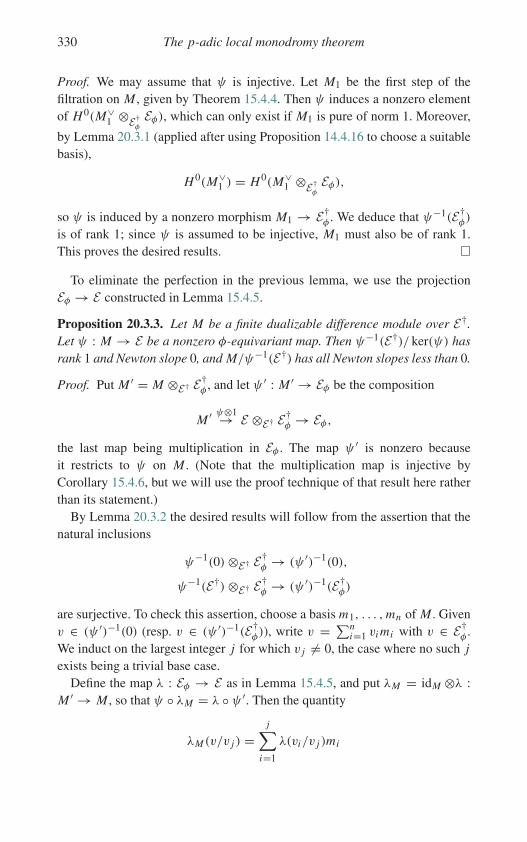
330 The p-adic local monodromy theorem
Proof. We may assume that ψ is injective. Let M1 be the first step of thefiltration on M , given by Theorem 15.4.4. Then ψ induces a nonzero elementof H0(M∨
1 ⊗E†φEφ), which can only exist if M1 is pure of norm 1. Moreover,
by Lemma 20.3.1 (applied after using Proposition 14.4.16 to choose a suitablebasis),
H0(M∨1 ) = H0(M∨
1 ⊗E†φEφ),
so ψ is induced by a nonzero morphism M1 → E†φ . We deduce that ψ−1(E†
φ)
is of rank 1; since ψ is assumed to be injective, M1 must also be of rank 1.This proves the desired results.
To eliminate the perfection in the previous lemma, we use the projectionEφ → E constructed in Lemma 15.4.5.
Proposition 20.3.3. Let M be a finite dualizable difference module over E†.Let ψ : M → E be a nonzero φ-equivariant map. Then ψ−1(E†)/ ker(ψ) hasrank 1 and Newton slope 0, and M/ψ−1(E†) has all Newton slopes less than 0.
Proof. Put M ′ = M ⊗E† E†φ , and let ψ ′ : M ′ → Eφ be the composition
M ′ ψ⊗1→ E ⊗E† E†φ → Eφ,
the last map being multiplication in Eφ . The map ψ ′ is nonzero becauseit restricts to ψ on M . (Note that the multiplication map is injective byCorollary 15.4.6, but we will use the proof technique of that result here ratherthan its statement.)
By Lemma 20.3.2 the desired results will follow from the assertion that thenatural inclusions
ψ−1(0)⊗E† E†φ → (ψ ′)−1(0),
ψ−1(E†)⊗E† E†φ → (ψ ′)−1(E†
φ)
are surjective. To check this assertion, choose a basis m1, . . . ,mn of M . Givenv ∈ (ψ ′)−1(0) (resp. v ∈ (ψ ′)−1(E†
φ)), write v = ∑ni=1 vi mi with v ∈ E†
φ .We induct on the largest integer j for which v j �= 0, the case where no such jexists being a trivial base case.
Define the map λ : Eφ → E as in Lemma 15.4.5, and put λM = idM ⊗λ :M ′ → M , so that ψ ◦ λM = λ ◦ ψ ′. Then the quantity
λM (v/v j ) =j∑
i=1
λ(vi/v j )mi
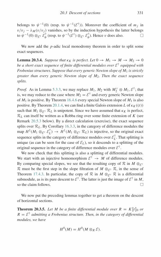
20.3 Descent of sections 331
belongs to ψ−1(0) (resp. to ψ−1(E†)). Moreover the coefficient of m j inv/v j − λM (v/v j ) vanishes, so by the induction hypothesis the latter belongsto ψ−1(0)⊗E† E†
φ (resp. to ψ−1(E†)⊗E† E†φ). Hence v does also.
We now add the p-adic local monodromy theorem in order to split someexact sequences.
Lemma 20.3.4. Suppose that κK is perfect. Let 0 → M1 → M → M2 → 0be a short exact sequence of finite differential modules over E† equipped withFrobenius structures. Suppose that every generic Newton slope of M1 is strictlygreater than every generic Newton slope of M2. Then the exact sequencesplits.
Proof. As in Lemma 5.3.3, we may replace M1,M2 with M∨2 ⊗ M1, E†; that
is, we may reduce to the case where M2 = E† and every generic Newton slopeof M1 is positive. By Theorem 16.4.6 every special Newton slope of M1 is alsopositive. By Theorem 20.1.4, we can find a finite Galois extension L of κK ((t))such that M1 ⊗E† RL is unipotent. Since we have assumed that κK is perfect,RL can itself be written as a Robba ring over some finite extension of K (seeRemark 20.5.3 below). By a direct calculation (exercise), the exact sequencesplits over RL . By Corollary 16.3.3, in the category of difference modules themap H1(M1 ⊗E† E†
L) → H1(M1 ⊗E† RL) is injective, so the original exact
sequence splits in the category of difference modules over E†L . That splitting is
unique (as can be seen for the case of EL ), so it descends to a splitting of theoriginal sequence in the category of difference modules over E†.
We now check that this splitting is also a splitting of differential modules.We start with an injective homomorphism E† → M of difference modules.By comparing special slopes, we see that the resulting copy of R in M ⊗E†
R must be the first step in the slope filtration of M ⊗E† R, in the sense ofTheorem 17.4.3. In particular, the copy of R in M ⊗E† R is a differentialsubmodule, as is its pure descent to E†. The latter is just the image of E† in M ,so the claim follows.
We now put the preceding lemmas together to get a theorem on the descentof horizontal sections.
Theorem 20.3.5. Let M be a finite differential module over R = K �t�0 orR = E† admitting a Frobenius structure. Then, in the category of differentialmodules, we have
H0(M) = H0(M ⊗R E).

332 The p-adic local monodromy theorem
Proof. For the case R = K �t�0 we have H0(M) = H0(M ⊗R E†) byProposition 17.2.5, so we may assume that R = E† hereafter. We may enlargeK to force κK to be perfect. We first check that any nonzero �-invarianthorizontal section v of M ⊗E† E descends to M . The section v correspondsto a nonzero φ-equivariant map ψ : M∨ → E . By Proposition 20.3.3,ψ−1(E†) �= 0 and the generic slopes of M∨/ψ−1(E†) are all negative. ByLemma 20.3.4 the exact sequence
0 → ψ−1(E†)/ ker(ψ)→ M∨/ ker(ψ)→ M∨/ψ−1(E†)→ 0
must split. However, again by Proposition 20.3.3, any complement ofψ−1(E†)/ ker(ψ) in M∨/ ker(ψ) that is in the category of difference modulesmust map to zero under ψ . We conclude that in fact ψ(M∨) = E†, forcingv ∈ H0(M).
To check the original claim (still for R = E†), we may enlarge K to havean algebraically closed residue field. In this case, Corollary 14.6.4 implies thatH 0(M ⊗E† E) is spanned by one-dimensional fixed subspaces for some powerof the Frobenius action. The previous argument shows that any generator ofone of these subspaces belongs to M , proving the claim.
20.4 Local duality
Here is another useful property of quasiunipotent differential modules, whichby Theorem 20.1.4 is present whenever one has a Frobenius structure.
Lemma 20.4.1. Put R = E† or R. Let M be a finite free differential moduleover R. Then, for i = 0, 1, the natural maps
Hi (M)→ Hi (M ⊗E† E†L)
GL/κK ((t))
are bijections.
Proof. For i = 0, we clearly have
H0(M ⊗E† E†L)
GL/κK ((t)) = H0((M ⊗E† E†L)
GL/κK ((t)) ) = H0(M).
For i = 1, we have injectivity because M is a direct summand of M ⊗E† E†L .
We have surjectivity, because if x ∈ M ⊗E† E†L represents a Galois-invariant
class in H1(M ⊗E† E†L) then the average of g(x) over g ∈ GL/κK ((t)) is an
element of M representing the same class.
Proposition 20.4.2. Suppose that κK is perfect. (This assumption can beremoved; see Section 20.5.) Let M be a finite free quasiunipotent differential

20.5 When the residue field is imperfect 333
module over R. Then the spaces H0(M), H1(M) are finite-dimensional, andthere is a perfect pairing
H0(M)× H1(M∨)→ H1(M ⊗ M∨)→ H1(R) ∼= Kdt
t.
In particular, by Theorem 20.1.4 this holds whenever M admits a Frobeniusstructure.
Proof. This is straightforward to check when M is unipotent (exercise). Ingeneral, we may choose a finite Galois extension L of κK ((t)) such that M ⊗RRL is unipotent. Since we have assumed that κK is perfect, RL can itself bewritten as a Robba ring over some finite extension of K (see Remark 20.5.3below), so the desired assertions hold for M ⊗R RL . We may then deduce thedesired results using Lemma 20.4.1. (See also [128, Proposition 4.26].)
This leads to the following result of Matsuda [169, Theorem 7.8].
Corollary 20.4.3 (Matsuda). Every indecomposable finite free quasiunipotentdifferential module over R has the form M ⊗ N with M quasiconstant and Nunipotent.
Proof. Exercise.
20.5 When the residue field is imperfect
We mentioned earlier (Remark 19.0.1) that the reader should assume that theresidue field κK of K is perfect. We now discuss the possible confusion arisingwhen this hypothesis is omitted.
Remark 20.5.1. The Cohen structure theorem asserts that if F is a completediscretely valued field of characteristic p > 0 then there exists an isomorphismF ∼= κF ((t)). However, this isomorphism is far from unique; it depends notonly on the choice of the series parameter t but also on the choice of embed-ding of the residue field κF into F . This choice is unique when κF is perfect(because in that case one has Teichmüller lifts; see the notes for Chapter 14),but not otherwise.
Example 20.5.2. Suppose that F = Fp(x)((t)). Then, for any y = ∑∞i=1 yi t i ,
there is an embedding Fp(x) ↪→ F given by x �→ x + y.
Remark 20.5.3. Suppose further that E is a finite separable extension of F . Bythe Cohen structure theorem, we can find copies of κE and κF inside E and F ,respectively, and use these to present E and F as power series fields (possibly
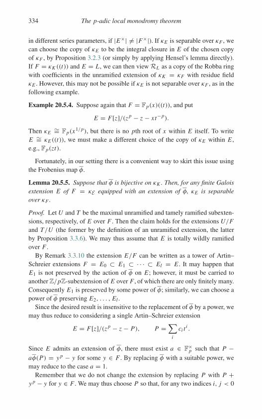
334 The p-adic local monodromy theorem
in different series parameters, if |E×| �= |F×|). If κE is separable over κF , wecan choose the copy of κE to be the integral closure in E of the chosen copyof κF , by Proposition 3.2.3 (or simply by applying Hensel’s lemma directly).If F = κK ((t)) and E = L , we can then view RL as a copy of the Robba ringwith coefficients in the unramified extension of κK = κF with residue fieldκE . However, this may not be possible if κE is not separable over κF , as in thefollowing example.
Example 20.5.4. Suppose again that F = Fp(x)((t)), and put
E = F[z]/(z p − z − xt−p).
Then κE ∼= Fp(x1/p), but there is no pth root of x within E itself. To writeE ∼= κE ((t)), we must make a different choice of the copy of κE within E ,e.g., Fp(zt).
Fortunately, in our setting there is a convenient way to skirt this issue usingthe Frobenius map φ.
Lemma 20.5.5. Suppose that φ is bijective on κK . Then, for any finite Galoisextension E of F = κE equipped with an extension of φ, κE is separableover κF .
Proof. Let U and T be the maximal unramified and tamely ramified subexten-sions, respectively, of E over F . Then the claim holds for the extensions U/Fand T/U (the former by the definition of an unramified extension, the latterby Proposition 3.3.6). We may thus assume that E is totally wildly ramifiedover F .
By Remark 3.3.10 the extension E/F can be written as a tower of Artin–Schreier extensions F = E0 ⊂ E1 ⊂ · · · ⊂ El = E . It may happen thatE1 is not preserved by the action of φ on E ; however, it must be carried toanother Z/pZ-subextension of E over F , of which there are only finitely many.Consequently E1 is preserved by some power of φ; similarly, we can choose apower of φ preserving E2, . . . , El .
Since the desired result is insensitive to the replacement of φ by a power, wemay thus reduce to considering a single Artin–Schreier extension
E = F[z]/(z p − z − P), P =∑
i
ci ti .
Since E admits an extension of φ, there must exist a ∈ F×p such that P −
aφ(P) = y p − y for some y ∈ F . By replacing φ with a suitable power, wemay reduce to the case a = 1.
Remember that we do not change the extension by replacing P with P +y p − y for y ∈ F . We may thus choose P so that, for any two indices i, j < 0
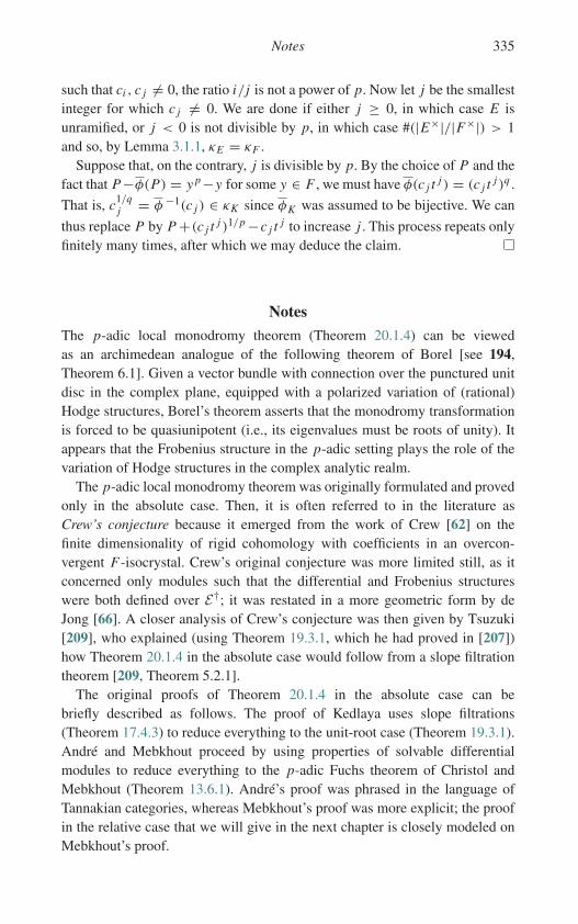
Notes 335
such that ci , c j �= 0, the ratio i/j is not a power of p. Now let j be the smallestinteger for which c j �= 0. We are done if either j ≥ 0, in which case E isunramified, or j < 0 is not divisible by p, in which case #(|E×|/|F×|) > 1and so, by Lemma 3.1.1, κE = κF .
Suppose that, on the contrary, j is divisible by p. By the choice of P and thefact that P−φ(P) = y p−y for some y ∈ F , we must have φ(c j t j ) = (c j t j )q .
That is, c1/qj = φ −1(c j ) ∈ κK since φK was assumed to be bijective. We can
thus replace P by P +(c j t j )1/p −c j t j to increase j . This process repeats onlyfinitely many times, after which we may deduce the claim.
Notes
The p-adic local monodromy theorem (Theorem 20.1.4) can be viewedas an archimedean analogue of the following theorem of Borel [see 194,Theorem 6.1]. Given a vector bundle with connection over the punctured unitdisc in the complex plane, equipped with a polarized variation of (rational)Hodge structures, Borel’s theorem asserts that the monodromy transformationis forced to be quasiunipotent (i.e., its eigenvalues must be roots of unity). Itappears that the Frobenius structure in the p-adic setting plays the role of thevariation of Hodge structures in the complex analytic realm.
The p-adic local monodromy theorem was originally formulated and provedonly in the absolute case. Then, it is often referred to in the literature asCrew’s conjecture because it emerged from the work of Crew [62] on thefinite dimensionality of rigid cohomology with coefficients in an overcon-vergent F-isocrystal. Crew’s original conjecture was more limited still, as itconcerned only modules such that the differential and Frobenius structureswere both defined over E†; it was restated in a more geometric form by deJong [66]. A closer analysis of Crew’s conjecture was then given by Tsuzuki[209], who explained (using Theorem 19.3.1, which he had proved in [207])how Theorem 20.1.4 in the absolute case would follow from a slope filtrationtheorem [209, Theorem 5.2.1].
The original proofs of Theorem 20.1.4 in the absolute case can bebriefly described as follows. The proof of Kedlaya uses slope filtrations(Theorem 17.4.3) to reduce everything to the unit-root case (Theorem 19.3.1).André and Mebkhout proceed by using properties of solvable differentialmodules to reduce everything to the p-adic Fuchs theorem of Christol andMebkhout (Theorem 13.6.1). André’s proof was phrased in the language ofTannakian categories, whereas Mebkhout’s proof was more explicit; the proofin the relative case that we will give in the next chapter is closely modeled onMebkhout’s proof.
336 The p-adic local monodromy theorem
For applications to rigid cohomology, as far as we know only the absolutecase of Theorem 20.1.4 is of any relevance. However, the nonabsolute caseoccurs in the context of relative p-adic Hodge theory. Namely, Berger andColmez [18] used the full strength of Theorem 20.1.4 to prove an analogue ofFontaine’s conjecture on the potential semistability of de Rham representations(Corollary 24.4.5 below) for a family of de Rham representations parametrizedby an affinoid base space.
To our knowledge, no proof of the nonabsolute case of Theorem 20.1.4 hasappeared prior to the one we are about to describe in Chapter 21. The proofby Kedlaya does not apply because it relies on Theorem 19.3.1, whose givenproof does not extend to the relative case. The use of the nonabsolute case ofTheorem 20.1.4 in [18] provided a strong motivation for working at this levelof generality in the present book.
Lemma 20.3.1 is a mild generalization of [206, Proposition 2.2.2]. A weakerresult in the same spirit appears in the work of Cherbonnier and Colmez [38].
For an absolute Frobenius lift, the case of Theorem 20.3.5 with R = E†
was originally conjectured by Tsuzuki [210, Conjecture 2.3.3] and proved byKedlaya [126, Theorem 1.1]. However, most of the ideas are already present inthe subcase R = K �t�0, which was established by de Jong [65, Theorem 9.1];the main difference is that de Jong could use Dwork’s trick (Corollary 17.2.2)where we had to use the p-adic local monodromy theorem (Theorem 20.1.4).Since a weak form of Dwork’s trick applies even without a differential struc-ture (Theorem 16.1.1), it should be possible to extend the case R = K �t�0 ofTheorem 20.3.5 to difference modules; this was carried out in the absolute casein [130], but we expect the general case to follow similarly.
The proof of Theorem 20.3.5 given here is in substance the same as theproof in the absolute case given in [126]. In particular, Proposition 20.3.3is essentially [126, Proposition 4.2], which in turn is close to de Jong’s [65,Corollary 8.2].
The original application of Theorem 20.3.5 in the case R = K �t�0 is deJong’s proof of the equal-characteristic analogue of Tate’s extension theoremon p-divisible groups (Barsotti–Tate groups). Tate proved [203] that for R acomplete discrete valuation ring of characteristic 0 and residual characteristicp > 0, given any two p-divisible groups over R, any morphism between theirgeneric fibres extends to a full morphism. Tate’s proof introduced the seeds thatgrew into the subject of p-adic Hodge theory (see Chapter 24); de Jong rec-ognized that an appropriate analogue of Tate’s method for R of characteristicp would proceed by means of crystalline Dieudonné theory. In this manner, deJong [65, Theorem 1.1] reduced this analogue of Tate’s theorem to an instanceof Theorem 20.3.5.

Exercises 337
The case R = E† of Theorem 20.3.5 has applications in the theory ofoverconvergent F-isocrystals (for more on which see Chapter 23). Namely,it implies (after some work) that, on a smooth variety over a field of charac-teristic p > 0, the restriction functor from overconvergent F-isocrystals toconvergent F-isocrystals is fully faithful [137, Theorem 4.2.1].
The local duality for quasiunipotent differential modules (Proposition 20.4.2)is due to Matsuda [169]. See also the treatment in [128, §4].
Exercises
(1) Prove that a finite free differential module M over R is quasiunipotent ifand only if M ⊗R RL is unipotent for some L . (Hint: produce a nonzeroquasiconstant submodule of M , e.g., by Galois descent.)
(2) Let 0 → M1 → M → M2 → 0 be a nonsplit extension of differentialmodules over R, where M1 and M2 are both trivial and of rank 1. Provethat M cannot admit a Frobenius structure that induces unit-root Frobeniusstructures on both M1 and M2. (Hint: use the fact that H1(R) = K dt/t .)
(3) Prove Lemma 20.3.1. (Hint: reduce to the case where |A|ρ ≤ 1 for someρ ∈ (0, 1) for which |w|ρ <∞. Then use |w|ρ to bound the terms of v ofnorm greater than some c > 0.)
(4) Complete the proof of Lemma 20.3.4 by proving the following assertion.Let M be a finite unipotent differential module over R, equipped with aFrobenius structure whose Newton slopes are all positive. Prove that anyexact sequence 0 → M → N → R → 0 in the category of differentialmodules with Frobenius structures must split. (Hint: apply Lemma 9.2.3 toN and then see how the resulting basis behaves under a standard Frobeniuslift.)
(5) In the notation of Theorem 20.3.5, suppose that φ(t) = tq . Prove that theequality H0(M) = H0(M ⊗R E) also holds in the category of differencemodules. (Hint: if v ∈ H0(M) then t−1 D(v) ∈ H0(M) also.)
(6) Prove Proposition 20.4.2 in the case where M is unipotent. (Hint: useLemma 9.2.3.)
(7) Prove Corollary 20.4.3 using Proposition 20.4.2. (Hint: let P be an inde-composable finite free quasiunipotent differential module over R. First,prove that P is a successive extension of copies of a single irreducible dif-ferential module M . Then construct an isomorphism P ∼= M ⊗ N , withN unipotent, by induction on the rank of P .)
21
The p-adic local monodromy theorem: proof
In this chapter we give a proof of the p-adic local monodromy theorem, atthe full level of generality at which we stated it (Theorem 20.1.4). After someinitial reductions, we start with the case of a module of differential slope 0,i.e., one satisfying the Robba condition. We describe how this case can betreated using either the p-adic Fuchs theorem for Christol–Mebkhout annuli(Theorem 13.6.1) or the slope filtration theorem of Kedlaya (Theorem 16.4.1).We then treat the rank 1 case using the classification of rank 1 solvable modulesfrom Chapter 12. We then show that any module of rank greater than 1 andprime to p can be made reducible, by comparing the module with its topexterior power and using properties of refined differential modules. We finallyhandle the case of a module M of rank divisible by p by considering M∨ ⊗ Minstead.
The reader may notice some similarities to the proof of the Turrittin–Levelt–Hukuhara decomposition theorem (Theorem 7.5.1). In fact, this theorem is alsoknown as the p-adic Turrittin theorem for this reason.
Besides the running hypothesis for this part of the book (Hypothesis 14.0.1)and the hypothesis from the previous chapter (Hypothesis 20.0.1), it will beconvenient to set several more hypotheses.
21.1 Running hypotheses
We are going to make a number of calculations under the same hypotheses.Rather than repeat the hypotheses each time, we enunciate them once and forall here. We first explain how to deal with the case where κK is imperfect.
Remark 21.1.1. First, we point out that it suffices to prove quasiunipotence,after replacing K by a complete extension K ′ to which φK extends, either by
338

21.2 Modules of differential slope 0 339
Proposition 6.9.1 or a more elementary argument (see [125, Proposition 6.11]).In particular we may take K ′ to be the φ-perfection of K , on which φ isbijective.
Here is a variant of the previous remark.
Remark 21.1.2. One can also proceed without φ-perfecting K initially butreplacing K by its inverse image under φ at any time when needed. We end upwith a finite extension L of φ−m(κK )((t)), for some positive integer m, suchthat M ⊗R RL is quasiunipotent. In particular, H0(M ⊗R RL) is a nonzerospace on which φ acts bijectively. Applying φm gives a nonzero element ofH0(M ⊗RRL ′) for a finite separable extension L ′ of κK ((t)). We may deducethat M has a nonzero �-stable differential submodule that is quasiunipotent;repeating this argument recovers Theorem 20.1.4 in full.
We are now ready to introduce the new running hypotheses mentioned in theintroduction to this chapter.
Hypothesis 21.1.3. For the rest of the chapter, assume that φK is bijectiveon K ; by the preceding remarks this is harmless for the purpose of prov-ing Theorem 20.1.4. Let F be a finite Galois (but not necessarily unramified)extension of K . Put RF = R⊗K F ; we will not attempt to extend φ to RF . LetM be a finite differential module over R equipped with a Frobenius structure.
Hypothesis 21.1.4. Within each lemma in this chapter, set the notation as fol-lows. Let N be a nonzero differential submodule (that is not a subquotient)of M ⊗R RF for some specified F . We will use L to indicate an initiallyunspecified finite separable extension of κK ((t)) to which φ extends; since φK
is bijective on K , Lemma 20.5.5 implies that RL may be viewed as a Robbaring over a finite unramified extension of K . We will use F ′ to indicate an ini-tially unspecified finite extension of F that is Galois over the integral closureK ′ of K in RL . (This may require the identification of a subfield of F largerthan K with an isomorphic subfield of RL .) Write RL ,F ′ = RL ⊗K ′ F ′.
Notation 21.1.5. We write N0 to refer to the component of N of differentialslope 0, as provided by Theorem 12.6.4.
21.2 Modules of differential slope 0
We start by describing objects of differential slope 0. This requires the useof either of two pieces of heavy machinery: the theory of p-adic exponents(Chapter 13) or the theory of slope filtrations for difference modules over theRobba ring (Theorem 17.4.3).
340 The p-adic local monodromy theorem: proof
Lemma 21.2.1. Suppose that N has differential slope 0. Then we may chooseL such that N ⊗RF RL ,F is unipotent.
Before giving either proof, we insert a reduction common to both.
Remark 21.2.2. In Lemma 21.2.1 the existence of N forces M to have a non-trivial summand M0 of differential slope 0, such that N appears in M ⊗RRF .It thus suffices to prove that if M is of differential slope 0 then we may chooseL such that M ⊗R RL is unipotent.
We first give the proof using p-adic exponents.
First proof of Lemma 21.2.1. As in Remark 21.2.2, we may assume that Mitself is of differential slope 0. By Corollary 17.3.2 we may change to astandard Frobenius lift. We may then apply Corollary 13.6.2 to deduce thatM ⊗R R[t1/m] is unipotent for some positive integer m coprime to p.
We next give the proof using slope filtrations.
Second proof of Lemma 21.2.1. Again as in Remark 21.2.2, we may assumethat M itself is of differential slope 0. By Theorem 17.4.3 (and changing theFrobenius lift, as in Corollary 17.3.2), we may reduce to the case where M ispure of norm 1 as a difference module.
In other words, Lemma 21.2.1 is reduced to the following claim. Let M bea finite differential module over E† admitting a unit-root Frobenius structurefor a standard Frobenius lift. Suppose that I R(M ⊗ Fρ) = 1 for ρ ∈ (0, 1)sufficiently close to 1. Then there exists a positive integer m coprime to p suchthat M ⊗R R[t1/m] is unipotent.
To prove this claim, apply Lemma 19.3.3 to construct a basis of M ⊗RE†[t1/m] for some m, on which�, t D act via matrices A, N such that A, A−1,
and N have entries in E† ∩ oK �t−1/m�. As in the proof of Lemma 19.3.4, thisforces N0 = 0.
For notational simplicity, assume hereafter that m = 1. Let f : K �t−1� →K �t� denote the substitution t−1 �→ t . We may then view f (N ) as defininga differential module M ′ over K 〈t/β〉 for the operator d/dt for some β > 1such that I R(M ′ ⊗K 〈t/β〉 Fβ) = 1. By Theorem 9.6.1 this module is trivial onthe open disc of radius β; this implies that the original module M is trivial, andin particular unipotent.
Remark 21.2.3. It would be interesting to know whether one can proveLemma 21.2.1 without using either p-adic exponents or slope filtrations butinstead simply using the fact that the hypothesis forces M to extend across
21.3 Modules of rank 1 341
the entire punctured open unit disc (by the pasting together of Frobeniusantecedents).
21.3 Modules of rank 1
We next consider the rank-1 case, using the classification of solvable rank 1differential modules (Theorem 12.7.2). This proof is the only point in thecourse of the proof of Theorem 20.1.4 at which we will introduce any spe-cific wildly ramified extensions of κK ((t)). (We made some tamely ramifiedextensions in Lemma 21.2.1 and will make some unramified extensions inLemma 21.4.1 below.)
Lemma 21.3.1. Suppose that rank(N ) = 1. Then we may choose L such thatN ⊗RF RL ,F is trivial.
Proof. We may assume that F contains all pth roots of 1. By Theorem 17.2.1,M is solvable at 1 as then is M ⊗R RF and also N . By Theorem 12.7.2 there
exists a nonnegative integer h such that N⊗phhas differential slope 0. If h = 0,
we may deduce the claim from Lemma 21.2.1. It suffices to check the caseh = 1, as we may apply this case repeatedly to deduce the general case.
In the case h = 1, by Theorem 17.1.6 (or the special case of the latterdiscussed in Remark 17.1.7), there exist c1, . . . , cb ∈ {0} ∪ o×F , with ci = 0whenever i is divisible by p, such that the rank 1 differential module N1 =M1,c1 ⊗ · · · ⊗ Mb,cb over RF has the property that N∨
1 ⊗ N has differentialslope 0. Since N1 ⊗RF RL0,F is unipotent for L0 equal to the Artin–Schreierextension L0 of κF ((t)) defined by the parameter c1t−1 + · · · + cbt−b, so isN ⊗RF RL0,F .
Unfortunately, this construction does not guarantee that L0 admits an actionof φ. However, suppose that we run over all possible choices of N for the givenM and F and define each L0 we see, using the unique possible Artin–Schreierparameter in the additive group ⊕
i<0,p�i
κalgK t−i .
The resulting parameters then fill out a finite set S.Pick an integer i with i < 0, p � i . Let Si be the set of coefficients of
t−i appearing in the elements of S. Let Pi (x) ∈ κK [x] be the product of thedistinct minimal polynomials of the elements of Si over κK . Since M admitsa Frobenius structure, the roots of φ(Pi (x)), when multiplied by t−qi , mustdefine Artin–Schreier parameters that are equivalent to the roots of Pi (x)whenmultiplied by t−i . In other words,
342 The p-adic local monodromy theorem: proof
φ(Pi (x)) = Pi (x1/q)q .
We may thus extend φ to the splitting field of Pi in such a way that, for eachroot a of Pi , we have φ(a) = bq for some root b of Pi .
This allows us to define a compositum of Artin–Schreier extensions L towhich φ extends; this includes all the choices of L0 made above. For suchan L , N ⊗RF RL ,F has differential slope 0, so we can make it trivial byLemma 21.2.1. This gives the desired result.
21.4 Modules of rank prime to p
We next pass from rank 1 to rank prime to p, using what we know about refineddifferential modules over Fρ .
Lemma 21.4.1. Suppose that rank(N ) is coprime to p. Then we may chooseL , F ′ such that N ⊗RF RL ,F ′ is either unipotent or reducible.
Proof. Put n = rank(N ). The case n = 1 is covered by Lemma 21.3.1, sowe may assume that n is greater than 1 and coprime to p. Suppose by way ofcontradiction that N ⊗RF RL ,F ′ is irreducible and nontrivial for all L , F ′. ByLemmas 21.2.1 and 21.3.1, we may reduce to the case where (M∨ ⊗ M)0 isunipotent and ∧n N is trivial.
Let us realize M,M0, N as differential modules on some annulus α < |t | <1. For ρ ∈ (α, 1), let Fρ = F�ρ/t, t/ρ�an, F ′
ρ = F ′�ρ/t, t/ρ�an denote thefields of analytic elements on the circle of radius ρ over the respective basefields F, F ′. We claim that N ⊗ Fρ must be refined for every ρ ∈ (α, 1).Otherwise, by Theorem 10.6.7, for a suitable choice of F ′ and some positiveinteger m coprime to p we could split N nontrivially over F ′
ρ(t1/m). Each
projector for this splitting would define a horizontal section of (N∨ ⊗ N ) ⊗F ′ρ(t
1/m). Since (M∨ ⊗ M)0 is unipotent, so is its subquotient (N∨ ⊗ N )0;consequently we would have
H0(N∨ ⊗ N ⊗ F ′ρ(t
1/m)) = H0(N∨ ⊗ N )
in terms of a basis of (N∨ ⊗ N )0, as in Lemma 9.2.3. We would thus get anontrivial splitting of N itself, contrary to hypothesis.
We now have that Nρ is refined for every ρ ∈ (α, 1). Choose ρ ∈ (α, 1) such
that p p−h/(p−1) < I R(N ⊗ Fρ) < p p−h+1/(p−1) for some nonnegative integerh. Apply Theorem 10.4.2 to form the h-fold Frobenius antecedent P of N⊗Fρ ,which is still refined. We may then apply Proposition 6.8.4(a) to deduce thatP⊗n has the same spectral radius as P and Proposition 6.8.4(b) to deduce that(∧n P∨)⊗P⊗n has a strictly greater spectral radius than P . However, these two
Notes 343
contradict each other because ∧n P∨ is the h-fold Frobenius antecedent of thetrivial module (∧n N∨)⊗ Fρ . This contradiction yields the desired result.
21.5 The general case
We now make the step from rank prime to p to arbitrary rank. The trick usedhere is one familiar from elementary group theory, e.g., it is used in the proofof the Sylow theorems. See the exercises for another example of its use.
Lemma 21.5.1. For arbitrary N, we may choose L , F ′ such that N⊗RF RL ,F ′is either unipotent or reducible.
Proof. By Lemma 21.4.1 it suffices to consider N of rank n divisible by p.Then the trace-0 component of N∨ ⊗ N has rank n2 − 1, which is not divis-ible by p. By repeated application of Lemma 21.4.1, we can force the trace-0component of (N∨⊗ N )⊗RF RL ,F ′ to acquire a unipotent component. In par-ticular, the space V = H 0((N∨ ⊗ N ) ⊗RF RL ,F ′) has F ′-dimension greaterthan 1.
We may view V as a finite-dimensional, not necessarily commutative, F ′-algebra. A standard fact about such algebras (exercise) is that, for some finiteextension F ′′ of F ′, V ⊗F ′ F ′′ fails to be a division algebra. Thus for suitableF ′′ we can find a pair of nonzero horizontal that endomorphisms of N ⊗RL ,F ′′which compose to zero. This forces N to be reducible.
Proof of Theorem 20.1.4. It suffices to consider M as irreducible. ByLemma 21.5.1, we may choose L , F ′ such that M⊗RRL ,F ′ is either unipotentor reducible. In the former case we are done, as this implies that M ⊗R RL isalso unipotent. Otherwise, M ⊗RRL ,F ′ contains a proper nonzero differentialsubmodule N . By applying Lemma 21.5.1 repeatedly, we may keep replacingN by a submodule (after changing L and F ′) until N becomes unipotent.
Apply� to (M ⊗RRL)⊗K ′ F ′ on the left and Gal(F ′/K ′) on the right. Theimages of N fill out a submodule of the form N0⊗K ′ F ′, where N0 is a nonzerodifferential submodule of M stable under �. The module N0 is unipotentbecause N0⊗K ′ F ′ is unipotent. Consequently M ⊗RRL has a nonzero unipo-tent submodule N0 stable under �, so we may apply the induction hypothesisto (M ⊗R RL)/N0 to conclude.
Notes
The approach to Theorem 20.1.4 presented here is modeled on that given byMebkhout [171] in the absolute case, except that Mebkhout describes only
344 The p-adic local monodromy theorem: proof
the first of our two proofs of Lemma 21.2.1. The approach of André [5] issubstantively similar but formally different, as it is phrased in the language ofTannakian categories.
In the course of proving Lemma 21.3.1, we noticed that if φ is not anabsolute Frobenius lift, then the condition of admitting an extension of φ isa highly nontrivial restriction on finite separable extensions of κK ((t)). Thisphenomenon was noted in the context of p-adic Hodge theory by Berger andColmez [18, Proposition 6.2.2].
Exercises
(1) Let G be a finite p-group and let τ : G → GL(V ) be a complex linearrepresentation of G. Prove that if τ is nontrivial then either τ or τ∨ ⊗τ has a nontrivial one-dimensional subrepresentation. (Hint: consider thepossible dimensions of irreducible representations of G.)
(2) Let V be a finite-dimensional, not necessarily commutative, F-algebra.Prove that there exists a finite extension F ′ of F such that V ⊗F ′ F is not adivision algebra. (Hint: we may assume that V itself is a division algebra.Pick any nonzero x ∈ V , view x as a linear transformation from V to Vvia left multiplication, and subtract an eigenvalue of this transformation.)

Part VI
Areas of Application

22
Picard–Fuchs modules
In this final part of the book, we touch briefly on some areas of application ofthe theory of p-adic differential equations. These chapters are intended more toinspire than to inform, with statements that are more illustrative than definitive.
In the present chapter we revisit the territory of Chapter 0, briefly discussinghow Picard–Fuchs modules give rise to differential equations with Frobeniusstructures and what this has to do with zeta functions.
22.1 Origin of Picard–Fuchs modules
The original source for p-adic differential equations, which inspired thegeneral theory, was the following construction.
Definition 22.1.1. Let K be a field of characteristic 0. Let t be a coordinateon the projective line P1
K . Let f : X → P1K be a proper, flat, generically
smooth morphism of algebraic varieties. Let S ⊂ P1K be a zero-dimensional
subscheme containing ∞ (for convenience) and all points over which f isnot smooth. The Picard–Fuchs modules on P1
K \ S associated with f are cer-tain finite locally free differential modules Mi for i = 0, . . . , 2 dim( f ) over�(P1
K \ S,O) with respect to the derivation d/dt ; they also have regular sin-gularities with rational exponents at each point of S. For λ /∈ S, the fibre ofMi at λ can be canonically identified with the i th de Rham cohomology of thefibre f −1(λ).
Although the classical construction of the Picard–Fuchs module is analytic(it involves viewing f as an analytically locally trivial fibration and integratingdifferentials against moving homology classes), there is an algebraic construc-tion, due to Katz and Oda [123], involving a Leray spectral sequence for thealgebraic de Rham cohomology of the total space.
347
348 Picard–Fuchs modules
Example 22.1.2. Perhaps the most fundamental example of a Picard–Fuchsmodule comes from the Legendre family of elliptic curves
y2 = x(x − 1)(x − t),
with S = {0, 1,∞}. In this case, the Picard–Fuchs module is precisely thedifferential module derived from the hypergeometric differential equation
y′′ + c − (a + b + 1)z
z(1 − z)y′ − ab
z(1 − z)y = 0,
with parameters (a, b, c) = (1/2, 1/2, 1), as considered in Chapter 0. See[213, §7] for an algebraic derivation of this fact, in the manner of Katzand Oda.
22.2 Frobenius structures on Picard–Fuchs modules
The example considered in Chapter 0 was just one of a number of explicitexamples studied by Dwork and others, in which there seemed to be somestrong relationship between the Picard–Fuchs equations derived in character-istic 0 and the zeta functions observed over finite fields. Dwork was able to givea somewhat systematic explanation, in some cases, in terms of Frobenius struc-tures; nowadays, the technology of p-adic cohomology (about which more inChapter 23) can be used to give a fairly general explanation.
We first give an explicit statement to the effect that Picard–Fuchs modulesalways carry Frobenius structures. See the notes for a more detailed discussion.
Theorem 22.2.1. With notation as above, assume that the field K is completefor a discrete valuation. Also suppose that f extends to a proper morphismX → P1
oKsuch that the intersection of P1
k with the nonsmooth locus is con-tained in the intersection of P1
k with the Zariski closure of S (i.e., the morphismis smooth over all points of P1
k that are not the reductions of points in S). Let Mi
be the ith Picard–Fuchs module for f , and let φ : P1oK
→ P1oK
be a Frobeniuslift (e.g., t �→ t p) that acts on oK as a lift of the absolute Frobenius morphism.Then, for some α ∈ (0, 1), there exists an isomorphism φ∗(Mi ) ∼= Mi over theFréchet completion R of �(P1
K \ S,O) for the ρ−1-Gauss norm and the Gaussnorms |t − λ| = ρ, ρ ∈ [α, 1) and λ ∈ S.
Remark 22.2.2. Geometrically, the Frobenius structure is defined on the com-plement in P1
K of a union of discs around the points of S, each of radius lessthan 1. (This includes a disc of radius less than 1 around ∞, by which we meanthe complement of a disc of radius greater than 1 around 0.) In particular, by
22.3 Relationship to zeta functions 349
working in a unit disc not containing any points of S, we obtain a differen-tial module with Frobenius structure over K �t�0. In a unit disc containing oneor more points of S, we obtain a differential module with Frobenius structureonly over ∪α>0 K 〈α/t, t�0. If the disc contains exactly one point of S and theexponents at that point are all 0, we can also obtain a differential module withFrobenius structure over K �t�0 for the derivation td/dt , provided that φ fixesthat point.
Example 22.2.3. In Example 22.1.2, Theorem 22.2.1 applies directly exceptwhen p = 2. In that case the reduction modulo p fails to be genericallysmooth; one must change the defining equation to get a usable descriptionmod 2.
22.3 Relationship to zeta functions
We next give an explicit statement to the effect that the Frobenius structure ona Picard–Fuchs module can be used to compute zeta functions. (The conditionon λ allows for a unique choice in each residue disc, by Lemma 15.2.6.)
Theorem 22.3.1. Retain the notation of Theorem 22.2.1, but now assume thatκK = Fq with q = pa and that φ is a qth-power Frobenius lift on P1
oK.
Suppose that λ ∈ oK satisfies φ(t − λ) ≡ 0 (mod t − λ) and that f extendssmoothly over the residue disc containing λ. Then
ζ( f −1(λ), T ) =2 dim( f )∏
i=0
det(1 − T�, (Mi )λ)(−1)i+1
.
This suggests an interesting strategy for computing zeta functions, whichwas described by Alan Lauder.
Remark 22.3.2. Suppose that we have in hand the differential module Mi ,plus the action of � on some individual (Mi )λ. (This data would ordinarily bespecified by a basis of Mi , the matrix of action of D, and the matrix of actionof � modulo t − λ.) View the equation
N A + d A
dt= dφ(t)
dtAφ(N )
as a differential equation with initial condition provided by (Mi )λ; we maythen solve for A and evaluate at another λ.
More explicitly, let us suppose for simplicity that λ = 0 is the starting valueand λ = 1 is the target value. In the open unit disc around 0, we can computeU such that
350 Picard–Fuchs modules
U−1 NU + U−1 dU
dt= 0
and then write down
A = U A0φ(U−1).
This gives only a power series representation around t = 0 with radius ofconvergence 1; it does not give any way in which we can specialize to λ = 1.
However, Theorem 22.2.1 implies that the entries of A can be written asuniform limits of rational functions with limited denominators. For the pur-poses of computing the zeta function, we can limit how much p-adic accuracyis needed in the computations by giving some bounds on the degrees of thepolynomials that appear and the sizes of the coefficients (e.g., using the Weilconjectures, Theorem 0.2.5). To obtain this much accuracy, we must computeA modulo some particular power of p. This means that we must determinesome rational function whose degree we can (in principle) control, so it suf-fices to determine suitably many terms in the power series expansion around0. We can then reconstruct a sufficiently good rational function approximationto A and evaluate at λ = 1.
Remark 22.3.3. One can recover from Theorem 22.3.1 the example of Dworkdiscussed in Chapter 0. In that example one is separating the Picard–Fuchsmodule, which has rank 2, into a unit-root component and a componentof slope log p. For this to be possible, one must be in the situation ofTheorem 15.3.4; this fails precisely at the residue discs at which the Igusapolynomial vanishes, which is why one must invert the Igusa polynomial inthe course of the computation.
Notes
The notion of algebraic de Rham cohomology was introduced by Grothendieckin [98], where he gave an algebraic construction of the topological de Rhamcohomology of a complex algebraic variety. The construction involves com-mingling the straightforward cohomology of the de Rham complex (con-structed from a module of Kähler differentials) with the cohomology ofcoherent algebraic sheaves. The subject was further developed by Hartshorne[105, 106]. A thorough treatment of Grothendieck’s theorem can be foundin [97].
In the final footnote to [98], Grothendieck gave what we believe was thefirst suggestion that one should consider in general what we call Picard–Fuchs
Notes 351
modules. His suggestion was based on Manin’s work on the Mordell conjec-ture over function fields; partly for this reason, Picard–Fuchs modules are alsocommonly known as Gauss–Manin connections. (This terminology is appar-ently due to Grothendieck. The name presumably refers to Gauss’s study ofhypergeometric differential equations, which incorporated the original Picard–Fuchs equation governing the periods of elliptic curves.) A good collection ofonward references can be found in [109].
The fact that a Picard–Fuchs module has regular singularities with rationalexponents can be proved in several ways, both geometric (Griffiths, Landman)and arithmetic (Katz). One can also formulate a more abstract version, con-cerning polarized variations of Hodge structures; this was proved by Borel andextended by Schmid (see the notes to Chapter 20 for further discussion of thislast point). Again, see [109] for references.
The construction of Frobenius structures on Picard–Fuchs modules is aconsequence of general results in the theory of p-adic cohomology, whichwe discuss further in the next chapter. For the moment we point out thatTheorem 22.2.1 in its stated form can be found in [211, Theorem 3.3.1].
Lauder’s strategy for computing zeta functions (also called the deforma-tion method) was introduced in [154]; it has been worked out in detail forhyperelliptic curves by Hubrechts [116]. Hubrechts implemented the resultingalgorithm in version 2.14 of the computer algebra system Magma. A versionfor hypersurfaces was described by Gerkmann [96].
23
Rigid cohomology
It has been suggested several times in this book that the study of p-adicdifferential equations is deeply connected with the theory of p-adic cohomol-ogy for varieties over finite fields. In particular, the Frobenius structures arisingon Picard–Fuchs modules, discussed in the previous chapter, appear within thistheory.
In this chapter, we introduce a little of the theory of rigid p-adic cohomol-ogy, as developed by Berthelot and others. In particular, we illustrate the roleplayed by the p-adic local monodromy theorem in a fundamental finitenessproblem in the theory.
23.1 Isocrystals on the affine line
We start with a concrete description of p-adic cohomology in a very specialcase, namely the cohomology of “locally constant” coefficient systems on theaffine line over a finite field. This is due to Crew [62].
Definition 23.1.1. Let k be a perfect (for simplicity) field of characteristic p >0. Let K be a complete discrete (again for simplicity) nonarchimedean field ofcharacteristic 0 with κK = k. An overconvergent F-isocrystal on the affine lineover k (with coefficients in K ) is a finite differential module with Frobeniusstructure on the ring A = ∪β>1 K 〈t/β〉, for some absolute Frobenius lift φ;as in Proposition 17.3.1 the resulting category is independent of the choice ofFrobenius lift.
Definition 23.1.2. Let M be an overconvergent F-isocrystal on the affineline over k. Let R be a copy of the Robba ring with series parameter t−1,so that we can identify A as a subring of R. (We can write explicitly R =∪β>1 K 〈β−1/t−1, t−1}.) Define
352
23.2 Crystalline and rigid cohomology 353
H0(A1k,M) = ker(D,M),
H1(A1k,M) = coker(D,M),
H0loc(A
1k,M) = ker(D,M ⊗A R),
H1loc(A
1k,M) = coker(D,M ⊗A R),
H1c (A
1K ,M) = ker(D,M ⊗A (R/A)),
H 2c (A
1K ,M) = coker(D,M ⊗A (R/A)).
By taking kernels and cokernels in the short exact sequence
0 → M → M ⊗A R → M ⊗A (R/A)→ 0
and applying the snake lemma, we get an exact sequence
0 → H0(A1k,M)→ H0
loc(A1k,M)→ H1
c (A1k,M)
→ H1(A1k,M)→ H1
loc(A1k,M)→ H2
c (A1k,M)→ 0.
Remark 23.1.3. Crew [62] showed that in this construction Hi computes therigid cohomology of M , Hi
c computes the rigid cohomology with compactsupports, and Hi
loc computes some sort of local cohomology at ∞.
Crew’s main result in this setting was the following.
Theorem 23.1.4 (Crew). The spaces Hi (A1k,M), Hi
c (A1k,M), Hi
loc(A1K ,M)
are all finite-dimensional over K . Moreover, the Poincaré pairings
Hi (A1k,M)× H2−i
c (A1k,M∨)→ H2
c (A1k,A) ∼= K ,
Hiloc(A
1k,M)× H1−i
loc (A1k,M∨)→ H1
loc(A1K ,A) ∼= K
are perfect.
The key ingredient is the fact that, by the p-adic local monodromy theorem(Theorem 20.1.4), M ⊗A R is quasiunipotent which implies the finitenessof Hi
loc(A1k,M). This further implies the finite dimensionalities, except for
H1c (A
1k,M) and H1(A1
k,M); however, these are related by a map with finite-dimensional kernel and cokernel. Moreover, they carry incompatible topolo-gies: the former is a Fréchet space while the latter is dual to a Fréchet space.This incompatibility can be resolved only if both spaces are finite-dimensional.
23.2 Crystalline and rigid cohomology
Next, we briefly discuss how the previous example fits into a broader theory ofp-adic cohomology, deferring most references to the notes.
354 Rigid cohomology
Motivated by the work of Dwork and also by related work of Monsky andWashnitzer, Grothendieck proposed a method of constructing an analogue ofalgebraic de Rham cohomology in positive characteristic. This was developedby Berthelot and Ogus into the theory of crystalline cohomology. An impor-tant example of this is the fact that if X is a smooth proper scheme over Zp
then the algebraic de Rham cohomology of X carries a Frobenius action thatcomputes the zeta function of the special fibre. (This generalizes to explainthe results on Frobenius structures and zeta functions discussed in the previouschapter.)
One defect of crystalline cohomology is that it gives a coherent cohomo-logy theory only for schemes over a finite field that are smooth and proper.By contrast, the work of Monsky and Washnitzer had given a good theoryfor smooth affine schemes. To fuse these theories, Berthelot introduced thetheory of rigid cohomology as well as a theory of locally constant coefficientobjects, overconvergent F-isocrystals. The example in the previous paragraphdemonstrates the computation of the cohomology of coefficients on the affineline; a theory of cohomology with compact supports, and a local cohomologytheory, are also demonstrated by Crew’s construction.
For trivial coefficients, it was shown by Berthelot that rigid cohomology hasall the desired properties of a Weil cohomology: finite dimensionality, Poincaréduality, Künneth formula, cycle class maps, the Lefschetz trace formula forFrobenius morphisms, etc. These were extended to nonconstant coefficientsby Kedlaya, using a relative version of Theorem 23.1.4.
Berthelot also suggested a theory of constructible coefficients, based onideas from the theory of algebraic D-modules. (These are modules over a ringof differential operators; they are the natural coefficient objects in algebraic deRham cohomology.) Recent work of Caro, Kedlaya, and Tsuzuki has shownthat they form a good theory of coefficients, enjoying the same formal proper-ties as their �-adic étale counterparts. For example, one can execute a proof ofthe Weil conjectures entirely using p-adic cohomology [132].
23.3 Machine computations
In recent years, interest has emerged in explicit computation of the zeta func-tions of algebraic varieties defined over finite fields. Some of this interesthas come from cryptography, in particular the use of the Jacobians of elliptic(and later hyperelliptic) curves over finite fields as “black box abelian groups”for certain public-key cryptography schemes (Diffie-Hellman, ElGamal). Forelliptic curves, a good method for doing this was proposed by Schoof [196]. Itamounts to computing the trace of the Frobenius morphism on the �-torsionpoints, the set of which is otherwise known as the étale cohomology with
Notes 355
F�-coefficients, for values of � small enough to determine uniquely the oneunknown coefficient of the zeta function within the range prescribed by theHasse–Weil bound.
It turns out to be somewhat more difficult to execute Schoof’s scheme forcurves of higher genus, as discovered by Pila [180]. One is forced to work withhigher-division polynomials in order to compute the torsion of the Jacobianof the curve; an interpretation in terms of étale cohomology is of little valuebecause the definition of étale cohomology is not intrinsically computable. (Itis easy to write down cohomology classes, but it is difficult to test two suchclasses for equality.)
It has been noticed by several authors that rigid cohomology is intrinsicallymore computable and so lends itself better to this sort of task. Specifically,Kedlaya [124] proposed an algorithm using rigid cohomology to compute thezeta function of a hyperelliptic curve over a finite field of small odd character-istic. The limitation to odd characteristic was lifted by Denef and Vercauteren[72]; the limitation to small characteristic was somewhat remedied by Harvey[108], who improved the dependence on the characteristic p from O(p) toO(p1/2+ε).
More recently, interest has emerged in considering also higher-dimensionalvarieties; this has come partly from potential applications in the study of mir-ror symmetry for Calabi–Yau varieties. In this case étale cohomology is of nohelp at all, since there is no geometric interpretation of Hi
et for i > 1 analo-gous to the interpretation for i = 1 in terms of the Jacobian. Rigid cohomologyshould still be computable, but relatively little progress has been made in mak-ing these computations practical (one exception being the treatment of smoothsurfaces in projective 3-space in [3]). It may be necessary to combine thesetechniques with Lauder’s deformation method (see Remark 22.3.2) to obtainthe best results.
Notes
Crew’s work, and subsequent work that builds on it (e.g., [131]), makes essen-tial use of nonarchimedean functional analysis, as was evident in the discussionof Theorem 23.1.4. We recommend Schneider’s book [195] as a user-friendlyintroduction to this topic.
For general surveys of the subject of p-adic cohomology, we recom-mend [117] (for crystalline cohomology only) and [141] (broader but moreadvanced). Also useful at this level of generality is Berthelot’s original articleoutlining the theory of rigid cohomology [22].
For the basics of crystalline cohomology, see [27] and references within(largely to Berthelot’s thesis [21]). For the work of Monsky and Washnitzer
356 Rigid cohomology
which motivated it, in addition to the original papers [172, 173, 174] there isalso a useful survey by van der Put [213].
Until recently no comprehensive introductory text on rigid cohomology wasavailable. That state of affairs was remedied by the appearance of the bookof Le Stum [157]. Berthelot’s own attempt at a foundational treatise remainsincomplete, but what does exist [23] may also be helpful. Some of the functionof a foundational text has been served by Berthelot’s articles concerning finitedimensionality [24] and Poincaré duality [25].
For coefficients in an overconvergent F-isocrystal, the basic properties(finite dimensionality, Poincaré duality, the Künneth formula) are proved in[131] using techniques similar to those of Crew in [62]. However, thesetechniques do not appear to suffice for the construction of a full coefficienttheory. For this, one needs a higher-dimensional analogue of Theorem 20.1.4,called the semistable reduction theorem for overconvergent F-isocrystals. Thisasserts that an overconvergent F-isocrystal on a noncomplete variety canalways be extended to a logarithmic isocrystal on some compactification, afterpulling back along a generically finite cover; such a result allows reductionsto arguments about (logarithmic) crystalline cohomology. (Except for the partof the theorem that concerns the cover, this is analogous to Deligne’s theoryof canonical extensions in [68].) See [134, 137, 140, 143] for the proof; theoriginal results from the present book feature prominently in [143].
Berthelot wrote a useful survey of his theory of arithmetic D-modules [26].It is this theory that has been developed by Caro (in part jointly with Tsuzuki)into a full theory of p-adic coefficients. This work is quite expansive andrequires a summary more detailed than we can provide here; see [35, 36] for arepresentative sample.
On the subject of machine calculations, as a companion to our original paperon hyperelliptic curves [124] we recommend Edixhoven’s course notes [83].Some discussion is also included in [93, Chapter 7]. We gave a condensedsummary of the general approach in [127]. For more on the role of elliptic andhyperelliptic curves in cryptography (including the relevance of the problem ofthe machine computation of zeta functions), the standard first reference is [55]even though it is some years behind the frontiers of this fast-moving subject.(For instance, it predates the growing area of pairing-based cryptography.)
24
p-adic Hodge theory
For our last application we turn to the subject of p-adic Hodge theory. Recallthat in Chapter 19 we described a “nonabelian Artin–Schreier” construction,giving an equivalence of categories between continuous representations of theabsolute Galois group of a positive characteristic local field on a p-adic vec-tor space and certain differential modules with Frobenius structures. In thischapter, we describe an analogous construction for the Galois group of amixed-characteristic local field. We also mention a couple of applications ofthis construction.
Hypothesis 24.0.1. Throughout this chapter, let K be a finite extension of Qp,let V be a finite-dimensional Qp-vector space, and let τ : G K → GL(V ) be acontinuous homomorphism for the p-adic topology on V .
24.1 A few rings
We begin with the “field of norms” construction of Fontaine and Wintenberger.
Definition 24.1.1. Put Kn = K (ζpn ) and K∞ = ∪n Kn . Let F = Frac W (κK )
and F ′ be the maximal subfields of K and K∞, respectively, that are unramifiedover Qp. Put HK = G K∞ and �K = G K∞/K = G K /HK .
Definition 24.1.2. Put o = oCp . Let E+ be the inverse limit of the system
· · · → o/po → o/po,
in which each map is the p-power Frobenius morphism (which is a ring homo-morphism). More explicitly, the elements of E+ are sequences (x0, x1, . . . )
of elements of o/po for which x pn+1 = xn for all n. In particular, for any
nonzero x ∈ E+, the quantity pnvp(xn) is the same for all n for which
357
358 p-adic Hodge theory
xn �= 0; we call this quantity v(x) and conventionally put v(0) = +∞. Chooseε = (ε0, ε1, . . . ) ∈ E+ with ε0 = 1 and ε1 �= 1. (This choice is somewhatanalogous to the choice of a square root of −1 in C.)
The following observations were made by Fontaine and Wintenberger [92].
Proposition 24.1.3. The following are true.(a) The ring E+ is a domain in which p = 0, with fraction field E =
E+[(ε − 1)−1].(b) The function v : E+ → [0,+∞] extends to a valuation on E under
which E is complete and oE = E+.
(c) The field E is the algebraic closure of κK ((ε − 1)). (The embedding ofκK ((ε − 1)) into E exists because v(ε − 1) = p/(p − 1) > 0.)
Definition 24.1.4. Let A be the ring of Witt vectors of E, i.e., the uniquecomplete discrete valuation ring with maximal ideal p and residue field E. Theuniqueness follows from the fact that E is algebraically closed, hence perfect.In particular, the p-power Frobenius morphism on E lifts to an automorphismφ of A. (See the notes for Chapter 14 for further discussion of Witt vectors.)
Definition 24.1.5. Each element of A can be uniquely written as the sum∑∞n=0 pn[xn], where xn ∈ E and [xn] denotes the Teichmüller lift of xn (the
unique lift of xn that has a pm th root in A for all positive integers m); notethat φ([x]) = [x p] = [x]p. We may thus equip A with a weak topology,in which a sequence xm = ∑∞
n=0 pn[xm,n] converges to zero if, for each n,v(xm,n) → +∞ as m → +∞. Let AQp be the completion of Zp[([ε] − 1)±]in A for the weak topology; as a topological ring, it is isomorphic to the ring oEdefined over the base field Qp with its own weak topology. It is also φ-stablebecause φ([ε]) = [ε]p.
Definition 24.1.6. Let A be the completion of the maximal unramifiedextension of AQp , viewed as a subring of A. Put
AK = AHK ,
where the right-hand side makes sense because we have chosen all the rings sofar in a functorial fashion, so that they indeed carry a G K -action. Note that AK
can be written as a ring of the form oE , but with coefficients in F ′ rather thanin Qp.
Definition 24.1.7. For any ring denoted with a boldface A so far, define thecorresponding ring with A replaced by B by tensoring over Zp with Qp. Forinstance, B = A ⊗Zp Qp is the fraction field of A.
24.2 (φ, �)-modules 359
24.2 (φ, �)-modules
We are now ready to describe the mechanism, introduced by Fontaine, for con-verting Galois representations into modules over various rings equipped withmuch simpler group actions.
Definition 24.2.1. Recall that V is a finite-dimensional vector space equippedwith a continuous G K -action. Put
D(V ) = (V ⊗Qp B)HK ;by the Hilbert–Noether theorem, D(V ) is a finite-dimensional BK -vectorspace, and the natural map D(V ) ⊗BK B → V ⊗Qp B is an isomorphism.Since we have taken only HK -invariants, D(V ) retains a semilinear action ofG K /HK = �K ; it also inherits an action of φ from B. That is, D(V ) is a(φ, �)-module over BK , i.e., a finite free BK -module equipped with semilin-ear φ and �K -actions that commute with each other. It is also étale, which is tosay the φ-action is étale (unit-root), because, as in Definition 19.2.4, one canfind a G K -invariant lattice in V .
Theorem 24.2.2 (Fontaine). The functor D, from the category of continuousrepresentations of G K on finite-dimensional Qp-vector spaces to the categoryof étale (φ, �)-modules over BK , is an equivalence of categories.
Proof. The inverse functor is
V = (D(V )⊗BK B)φ=1.
The argument is similar to that in the proof of Proposition 19.1.5; see [89].
In much the same way that Proposition 19.1.5 was refined byTheorem 19.3.1, Theorem 24.2.2 was refined by Cherbonnier and Colmez asfollows [38]. The big difference is that no additional restriction on the Galoisrepresentations is imposed.
Definition 24.2.3. Let B†Qp
be the image of the bounded Robba ring E†, underthe identification of E (having coefficients in Qp) with BQp , sending t to [ε]−1. Let B†
K be the integral closure of B†Qp
in BK . Again, B†K carries the actions
of φ and �K .
Definition 24.2.4. Let A† be the set of x = ∑∞n=0 pn[xn] ∈ A such that
lim infn→∞ {v(xn)/n} > −∞.
DefineD†(V ) = (V ⊗Qp B†)HK ;
it is an étale (φ, �)-module over B†K .
360 p-adic Hodge theory
The following is the main result of [38].
Theorem 24.2.5 (Cherbonnier–Colmez). The functor D†, from the categoryof continuous representations of G K on finite-dimensional Qp-vector spaces tothe category of étale (φ, �)-modules over B†
K , is an equivalence of categories.
Remark 24.2.6. By Theorem 24.2.2, to check Theorem 24.2.5 it suffices tocheck that the base extension functor from étale (φ, �)-modules over B†
Kto étale (φ, �)-modules over BK is an equivalence. The full faithfulness ofthis functor is elementary and it follows from Lemma 16.3.2. The essentialsurjectivity is much deeper; it amounts to the fact that the natural map
D†(V )⊗B†K
B† → V ⊗Qp B†
is an isomorphism. Verifying this requires the development of an appropriateanalogy to Sen’s theory of decompletion; this analogy has been developed intoa full abstract Sen theory by Berger and Colmez [18].
A further variant was proposed by Berger [14].
Definition 24.2.7. Using the identification B†Qp
∼= E†, put
B†rig,K = B†
K ⊗B†Qp
R,
where R is the Robba ring over Qp; the subscript “rig” indicates “rigid” inthe sense of rigid analytical geometry. Note that B†
rig,K admits continuousextensions (for the LF-topology) of the actions of φ and �K . Define
D†rig(V ) = D†(V )⊗B†
KB†
rig,K ;
it is an étale (φ, �)-module over B†rig,K .
Theorem 24.2.8 (Berger). The functor D†rig, from the category of continuous
representations of G K on finite-dimensional Qp-vector spaces to the categoryof étale (φ, �)-modules over B†
rig,K , is an equivalence of categories.
Remark 24.2.9. The principal new content in Theorem 24.2.8 is that the baseextension functor from étale φ-modules over E† to étale φ-modules over R isfully faithful; this follows from Corollary 16.3.4. The essential surjectivity ofthe functor is almost trivial, since the étaleness of the φ-action is defined overthe Robba ring by base extension from E† (Definition 16.3.1). One need onlycheck that the �K -action also descends to any étale lattice, but this is easy: theproof is similar to that of Lemma 17.4.2.

24.3 Galois cohomology 361
24.3 Galois cohomology
Since the functor D and its variants lose no information about Galois represen-tations, it is unsurprising that they can be used to recover basic invariants of arepresentation, such as its Galois cohomology.
Definition 24.3.1. Assume for simplicity that �K is procyclic; this eliminatesonly the case where p = 2 and {±1} ⊂ �, for which see Remark 24.3.2below. Let γ be a topological generator of �. Define the Herr complex overBK associated with V as the complex (with the first nonzero term placed indegree 0)
0 → D(V )→ D(V )⊕ D(V )→ D(V )→ 0;here the first map is m �→ ((φ−1)m, (γ −1)m) and the second is (m1,m2)→(γ − 1)m1 − (φ − 1)m2. (The fact that this is a complex follows from thecommutativity of φ and γ .) Similarly, define the Herr complex over B†
K or
B†rig,K by replacing D(V ) by D†(V ) or D†
rig(V ), respectively.
Remark 24.3.2. In a more conceptual description, which also covers the casewhere �K need not be profinite, one takes the total complex associated with
0 → C ·(�K , D(V ))φ−1→ C ·(�K , D(V ))→ 0,
where C ·(�K , D(V )) is the usual cochain complex for computing Galoiscohomology (as in [199, §I.2.2]). One might think of this as the “monoidcohomology” of �K × φZ≥0 acting on D(V ).
Theorem 24.3.3. The cohomology of the Herr complex computes the Galoiscohomology of V .
Proof. For BK , the desired result was established by Herr [111]. The argumentproceeds in two steps. One takes first the cohomology of the Artin–Schreiersequence
0 → Qp → Bφ−1→ B → 0,
after tensoring with V . This reduces the claim to the fact that the inflationhomomorphisms
Hi (�K , D(V ))→ Hi (G K , V ⊗Qp B)
are bijections; this is proved by adapting a technique introduced by Sen.For B†
K and B†rig,K , the desired result was established by Liu [160]; his argu-
ment proceeds by comparison with the original Herr complex rather than byimitation of the above argument, though one could probably do that also.
362 p-adic Hodge theory
Remark 24.3.4. As in [111, 160], one can make Theorem 24.3.3 more precise.For instance, the construction of Galois cohomology is functorial; there is alsoan interpretation in the Herr complex of the cup product in cohomology.
Remark 24.3.5. One can also use the Herr complex to recover Tate’s fun-damental theorems on Galois cohomology (finite dimensionality, the Euler–Poincaré characteristic formula, local duality). This was done by Herr in [112].
24.4 Differential equations from (φ, �)-modules
One of the original goals of p-adic Hodge theory was to associate finer invari-ants with p-adic Galois representations, so as, for instance, to distinguish thoserepresentations which arise in geometry (i.e., from the étale cohomology ofvarieties over K ). This was originally done using a collection of “period rings”introduced by Fontaine; more recently, Berger’s work has demonstrated thatone can reproduce these constructions using (φ, �)-modules. Here is a briefdescription of an example that shows the relevance of p-adic differential equa-tions to this study. We will make reference to Fontaine’s rings BdR,Bst withoutgiving definitions of them, for which see [15].
Definition 24.4.1. Let χ : �K → Z×p denote the cyclotomic character; that is,
for all nonnegative integers m and all γ ∈ �K ,
γ (ζpm ) = ζχ(γ )pm .
For γ ∈ �K sufficiently close to 1, we may compute
∇ = log γ
logχ(γ )
as an endomorphism of D(V ), using the power series for log(1+x). The resultdoes not depend on γ .
Remark 24.4.2. If one views �K as a one-dimensional p-adic Lie group overZp then ∇ is the action of the corresponding Lie algebra.
Definition 24.4.3. Note that ∇ acts on B†rig,K with respect to
f �→ [ε] log[ε] d f
d[ε] .
As a result, it does not induce a differential module structure with respectto d/dt on D(V ), but only on D(V ) ⊗ B†
rig,K [(log[ε])−1]. We say that V isde Rham if there exists a differential module with Frobenius structure M overB†
rig,K and an isomorphism
24.5 Beyond Galois representations 363
D(V )⊗ B†rig,K [(log[ε])−1] → M ⊗ B†
rig,K [(log[ε])−1]of differential modules with Frobenius structure.
One then has the following results of Berger [14].
Theorem 24.4.4 (Berger).(a) The representation V is de Rham if and only if it is de Rham in
Fontaine’s sense, i.e., if
DdR(V ) = (V ⊗Qp BdR)G K
satisfies
DdR(V )⊗K BdR ∼= V ⊗Qp BdR.
(b) Suppose that V is de Rham. If V is semistable in Fontaine’s sense,i.e., if
Dst(V ) = (V ⊗Qp Bst)G K
satisfies
Dst(V )⊗F Bst ∼= V ⊗Qp Bst
then there exists an M as in Definition 24.4.3 that is unipotent. Con-versely, if such an M exists then V is potentially semistable, i.e., itbecomes semistable upon restriction to GL for some finite extensionL of K .
Applying Theorem 20.1.4 then yields the following corollary, which waspreviously a conjecture of Fontaine [90, 6.2].
Corollary 24.4.5 (Berger). Every de Rham representation is potentiallysemistable.
Remark 24.4.6. The descriptor “de Rham” is meant to convey the fact thatif V = Hi
et(X ×K K alg,Qp) for X a smooth proper variety over K thenV is de Rham and one can use the aforementioned constructions to recoverHi
dR(X, K ) functorially from V (solving Grothendieck’s “problem of themysterious functor”). See [15] for more of this story.
24.5 Beyond Galois representations
The category of arbitrary (φ, �)-modules over B†rig,K turns out to have its own
representation-theoretic interpretation: it is equivalent to the category of B-pairs introduced by Berger [16]. One can associate “Galois cohomology” with
364 p-adic Hodge theory
such objects using the Herr complex; it has been shown by Liu [160] that theanalogues of Tate’s theorems (see Remark 24.3.5) still hold. These functorscan be interpreted as the derived functors of Hom(D†
rig(V0), ·) when V0 is thetrivial representation [142, Appendix].
It may be wondered why we should be interested in (φ, �)-modules overB†
rig,K if ultimately we have in mind an application concerning only Galoisrepresentations. One answer is that converting Galois representations into(φ, �)-modules exposes extra structure that is not visible without such aconversion.
Definition 24.5.1 (Colmez). We say that V is trianguline if D†rig(V ) is a
successive extension of (φ, �)-modules of rank 1 over B†rig,K . The point is
that these need not be étale, so V need not be a successive extension ofrepresentations of dimension 1.
Trianguline representations have the dual benefits of being relatively easy toclassify and also somewhat commonplace. On one hand, Colmez [58] classi-fied the two-dimensional trianguline representations of GQp ; the classificationincluded a parameter (the L-invariant) relevant to p-adic L-functions. Onthe other hand, a result of Kisin [146] shows that the Galois representationsassociated with many classical modular forms are in fact trianguline.
Notes
Our presentation here was largely a summary of Berger’s [15], which we highlyrecommend. For detailed study, the recent notes by Brinon and Conrad for the2009 Clay Mathematics Institute summer school [32] may be of considerablevalue.
A variant of the theory of (φ, �)-modules was introduced by Kisin [147],using the Kummer tower K (p1/pn
) instead of the cyclotomic tower K (ζpn ).This leads to certain advantages, particularly when studying crystalline rep-resentations. For instance, Kisin was able to use his construction to establishsome classification theorems for finite flat group schemes and for p-divisiblegroups, as conjectured by Breuil. Kisin’s work was based on an earlier paperof Berger [17]; both of these use slope filtrations (as in Theorem 16.4.1)to recover a theorem of Colmez and Fontaine classifying semistable Galoisrepresentations in terms of certain linear algebraic data.
After [14] had appeared, Fontaine succeeded in giving a direct proof ofCorollary 24.4.5 that did not involve p-adic differential equations; see [91].
References
[1] A. Abbes and T. Saito, Ramification of local fields with imperfect residue fields, Amer. J.Math. 124 (2002), 879–920.
[2] A. Abbes and T. Saito, Ramification of local fields with imperfect residue fields, II, Doc.Math. extra vol. (2003), 5–72.
[3] T. G. Abbott, K. S. Kedlaya, and D. Roe, Bounding Picard numbers of surfaces usingp-adic cohomology, in Arithmetic, Geometry and Coding Theory (AGCT 2005), SocietéMathématique de France, 2009, pp. 125–159.
[4] Y. André, Différentielles non commutatives et théorie de Galois différentielle ou auxdifférences, Ann. Sci. École Norm. Sup. (4) 34 (2001), 685–739.
[5] Y. André, Filtrations de type Hasse–Arf et monodromie p-adique, Invent. Math. 148 (2002),285–317.
[6] Y. André, Dwork’s conjecture on the logarithmic growth of solutions of p-adic differentialequations, Compos. Math. 144 (2008), 484–494.
[7] Y. André and F. Baldassarri, De Rham Cohomology of Differential Modules on AlgebraicVarieties, Progress in Math. 189, Birkhäuser, 2001.
[8] Y. André and L. Di Vizio, q-difference equations and p-adic local monodromy, Astérisque296 (2004), 55–111.
[9] M. F. Atiyah and I. G. Macdonald, Introduction to Commutative Algebra, Addison-Wesley,Reading, 1969.
[10] F. Baldassarri, Continuity of the radius of convergence of differential equations on p-adicanalytic curves, arXiv:0809.2479v3 (2009).
[11] F. Baldassarri and L. Di Vizio, Continuity of the radius of convergence of p-adic differentialequations on Berkovich analytic spaces, arXiv:0709.2008v3 (2008).
[12] M. Baker and R. Rumely, Potential Theory and Dynamics on the Berkovich Projective Line,Math. Surveys and Monographs 159, Amer. Math. Soc., 2010.
[13] A. Beilinson, S. Bloch, and H. Esnault, ε-factors for Gauss–Manin determinants, MoscowJ. Math. 2 (2002), 477–532.
[14] L. Berger, Représentations p-adiques et équations différentielles, Invent. Math. 148 (2002),219–284.
[15] L. Berger, An introduction to the theory of p-adic representations, in Geometric Aspects ofDwork Theory, Vols. I, II, de Gruyter, Berlin, 2004, 255–292.
[16] L. Berger, Construction de (ϕ, �)-modules: représentations p-adiques et B-paires, Algebraand Num. Theory 2 (2008), 91–120.
[17] L. Berger, Équations différentielles p-adiques et (φ, N )-modules filtrés, Astérisque 319(2008), 13–38.
[18] L. Berger and P. Colmez, Familles de représentations de de Rham et monodromie p-adique,Astérisque 319 (2008), 303–337.
365
366 References
[19] V. G. Berkovich, Spectral Theory and Analytic Geometry over Non-Archimedean Fields,Math. Surveys and Monographs 33, Amer. Math. Soc., Providence, 1990.
[20] V. G. Berkovich, Étale cohomology for non-Archimedean analytic spaces, Publ. Math. IHÉS78 (1993), 5–161.
[21] P. Berthelot, Cohomologie Cristalline des Schémas de Caractéristique p > 0, Lecture Notesin Math. 407, Springer-Verlag, Berlin, 1974.
[22] P. Berthelot, Géométrie rigide et cohomologie des variétés algébriques de caractéristiquep, in Introductions aux cohomologies p-adiques (Luminy, 1984), Mém. Soc. Math. France(N.S.) 23 (1986), 7–32.
[23] P. Berthelot, Cohomologie rigide et cohomologie rigide à support propre. Première par-tie, Prépublication IRMAR 96-03, available at http://perso.university-rennes1.fr/pierre.berthelot/.
[24] P. Berthelot, Finitude et pureté cohomologique en cohomologie rigide (with an appendix inEnglish by A. J. de Jong), Invent. Math. 128 (1997), 329–377.
[25] P. Berthelot, Dualité de Poincaré et formule de Künneth en cohomologie rigide, C.R. Acad.Sci. Paris 325 (1997), 493–498.
[26] P. Berthelot, Introduction à la théorie arithmétique des D-modules, cohomologies p-adiqueset applications arithmétiques, II, Astérisque 279 (2002), 1–80.
[27] P. Berthelot and A. Ogus, Notes on Crystalline Cohomology, Princeton University Press,Princeton, 1978.
[28] R. Bhatia, Matrix Analysis, Graduate Texts in Math. 169, Springer-Verlag, New York,1997.
[29] J. M. Borger, Conductors and the moduli of residual perfection, Math. Annalen 329(2004), 1–30.
[30] S. Bosch, Lectures on formal and rigid geometry, preprint (2008) available athttp://wwwmath1.uni-muenster.de/sfb/about/publ/bosch.html.
[31] S. Bosch, U. Güntzer, and R. Remmert, Non-Archimedean Analysis, Grundlehren der Math.Wiss. 261, Springer-Verlag, Berlin, 1984.
[32] O. Brinon and B. Conrad, p-adic Hodge theory, notes from the 2009 Clay MathematicsInstitute summer school, available online at http://math.stanford.edu/ ˜conrad/.
[33] S. Boucksom, C. Favre, and M. Jonsson, Valuations and plurisubharmonic singularities,Publ. Res. Inst. Math. Sci. 44 (2008), 449–494.
[34] K. Buzzard and F. Calegari, Slopes of overconvergent 2-adic modular forms, Compos. Math.141 (2005), 591–604.
[35] D. Caro, F-isocristaux surconvergents et surcohérence différentielle, Invent. Math. 170(2007), 507–539.
[36] D. Caro, Dévissages des F-complexes de D-modules arithmétiques en F-isocristauxsurconvergents, Invent. Math. 166 (2006), 397–456.
[37] N. L. Carothers, A Short Course on Banach Space Theory, Cambridge University Press,2004.
[38] F. Cherbonnier and P. Colmez, Représentations p-adiques surconvergentes, Invent. Math.133 (1998), 581–611.
[39] B. Chiarellotto and G. Christol, On overconvergent isocrystals and F-isocrystals of rankone. Compos. Math. 100 (1996), 77–99.
[40] B. Chiarellotto and A. Pulita, Arithmetic and Differential Swan conductors of rank onerepresentations with finite local monodromy, arXiv:0711.0701v1 (2007); to appear in Amer.J. Math.
[41] B. Chiarellotto and N. Tsuzuki, Logarithmic growth and Frobenius filtrations for solutionsof p-adic differential equations, J. Inst. Math. Jussieu 8 (2009), 465–505.
[42] G. Christol, Modules Différentiels et Equations Différentielles p-adiques, Queen’s Papersin Pure and Applied Math. 66, Queen’s University, Kingston, 1983.
References 367
[43] G. Christol, Un théorème de transfert pour les disques singuliers réguliers, in Cohomologiep-adique, Astérisque 119–120 (1984), 151–168.
[44] G. Christol, About a Tsuzuki theorem, in p-adic Functional Analysis (Ioannina, 2000),Lecture Notes in Pure and Appl. Math. 222, Dekker, New York, 2001, 63–74.
[45] G. Christol, Thirty years later, in Geometric Aspects of Dwork Theory, Vol. I, de Gruyter,Berlin, 2004, 419–436.
[46] G. Christol, Le Théorème de Turritin p-adique, in preparation; draft available at http://people.math.jussieu.fr/∼christol.
[47] G. Christol and B. Dwork, Effective p-adic bounds at regular singular points, Duke Math.J. 62 (1991), 689–720.
[48] G. Christol and B. Dwork, Differential modules of bounded spectral norm, in p-adic Meth-ods in Number Theory and Algebraic Geometry, Contemp. Math. 133, Amer. Math. Soc.,Providence, 1992.
[49] G. Christol and B. Dwork, Modules différentielles sur les couronnes, Ann. Inst. Fourier 44(1994), 663–701.
[50] G. Christol and Z. Mebkhout, Sur le théorème de l’indice des équations différentielles, II,Annals of Math. 146 (1997), 345–410.
[51] G. Christol and Z. Mebkhout, Sur le théorème de l’indice des équations différentielles, III,Annals of Math. 151 (2000), 385–457.
[52] G. Christol and Z. Mebkhout, Sur le théorème de l’indice des équations différentielles, IV,Invent. Math. 143 (2001), 629–672.
[53] R. C. Churchill and J. J. Kovacic, Cyclic vectors, in Differential Algebra and Related Topics(Newark, NJ, 2000), World Scientific, River Edge NJ, 2002, 191–218.
[54] D. Clark, A note on the p-adic convergence of solutions of linear differential equations,Proc. Amer. Math. Soc. 17 (1966), 262–269.
[55] H. Cohen and G. Frey (eds.), Handbook of Elliptic and Hyperelliptic Curve Cryptography,Discrete Math. and its Applications 34, Chapman & Hall/CRC, 2005.
[56] R. M. Cohn, Difference Algebra, John Wiley & Sons, New York, London, Sydney, 1965.[57] R. F. Coleman, Dilogarithms, regulators and p-adic L-functions, Invent. Math. 69 (1982),
171–208.[58] P. Colmez, Représentations triangulines de dimension 2, Astérisque 319 (2008), 213–258.[59] B. Conrad, Several approaches to non-archimedean geometry, in M. Baker et al.
(eds.), p-adic Geometry: Lectures from the 2007 Arizona Winter School, University Lec-ture Series 45, Amer. Math. Soc., 2008.
[60] F. T. Cope, Formal solutions of irregular linear differential equations, II, Amer. J. Math. 58(1936), 130–140.
[61] R. Crew, F-isocrystals and p-adic representations, in Algebraic Geometry (Brunswick,Maine, 1985), Proc. Symp. Pure Math. 46, Part 2, Amer. Math. Soc., Providence, 1987,111–138.
[62] R. Crew, Finiteness theorems for the cohomology of an overconvergent isocrystal on a curve,Ann. Sci. Éc. Norm. Sup. 31 (1998), 717–763.
[63] R. Crew, Canonical extensions, irregularities, and the Swan conductor, Math. Ann. 316(2000), 19–37.
[64] N. E. Csima, Newton–Hodge filtration for self-dual F-crystals, arXiv:0706/2530v1 (2007).[65] A. J. de Jong, Homomorphisms of Barsotti–Tate groups and crystals in positive characteris-
tic, Invent. Math. 134 (1998), 301–333; erratum, ibid. 138 (1999), 225.[66] A. J. de Jong, Barsotti–Tate groups and crystals, in Proc. Int. Congress of Mathematicians,
Vol. II (Berlin, 1998), Doc. Math. Extra Vol. II (1998), 259–265.[67] A. J. de Jong and F. Oort, Purity of the stratification by Newton polygons, J. Amer. Math.
Soc. 13 (2000), 209–241.[68] P. Deligne, Equations Différentielles à Points Singuliers Réguliers, Lecture Notes in Math.
163, Springer-Verlag, Berlin, 1970.
368 References
[69] P. Deligne, La conjecture de Weil, II, Publ. Math. IHÉS 52 (1980), 137–252.[70] P. Deligne and N. Katz (eds.), Groupes de Monodromie en Géométrie Algébrique II, Proc.
Séminaire de Géométrie Algébrique du Bois-Marie 1967–1969 (SGA 7 II), Lecture Notes inMath. 340, Springer-Verlag, Berlin, New York, 1973.
[71] M. Demazure, Lectures on p-divisible Groups, Lecture Notes in Math. 302, Springer-Verlag, New York, 1972.
[72] J. Denef and F. Vercauteren, An extension of Kedlaya’s algorithm to hyperelliptic curves incharacteristic 2, J. Cryptology 19 (2006), 1–25.
[73] L. Di Vizio, Local analytic classification of q-difference equations with |q| = 1, J. Non-commutative Geom. 3 (2009), 125–149.
[74] B. Dwork, p-adic cycles, Publ. Math. IHÉS 37 (1969), 27–115.[75] B. Dwork, On p-adic differential equations, II. The p-adic asymptotic behavior of solutions
of ordinary linear differential equations with rational function coefficients, Ann. Math. (2)98 (1973), 366–376.
[76] B. Dwork, On p-adic differential equations, III. On p-adically bounded solutions of ordi-nary linear differential equations with rational function coefficients, Invent. Math. 20 (1973),35–45.
[77] B. Dwork, Bessel functions as p-adic functions of the argument, Duke Math. J. 41 (1974),711–738.
[78] B. Dwork, Lectures on p-adic Differential Equations, Grundlehren der Math. Wissens-chaften 253, Springer-Verlag, New York, 1982.
[79] B. M. Dwork, On exponents of p-adic differential modules, J. reine angew. Math. 484(1997), 85–126.
[80] B. Dwork, G. Gerotto, and F. Sullivan, An Introduction to G-Functions, Ann. Math. Studies133, Princeton University Press, Princeton, 1994.
[81] B. Dwork and P. Robba, On ordinary linear p-adic differential equations, Trans. Amer. Math.Soc. 231 (1977), 1–46.
[82] B. Dwork and P. Robba, Effective p-adic bounds for solutions of homogeneous lineardifferential equations, Trans. Amer. Math. Soc. 259 (1980), 559–577.
[83] B. Edixhoven, Point counting after Kedlaya, course notes (2006) available at http://www.math.leidenuniv.nl/ ˜edix/oww/mathofcrypt/carls_edixhoven/kedlaya.pdf.
[84] D. Eisenbud, Commutative Algebra with a View Toward Algebraic Geometry, GraduateTexts in Math. 150, Springer-Verlag, New York, 1995.
[85] P. Enflo, A counterexample to the approximation problem in Banach spaces, Acta Math. 130(1973), 309–317.
[86] G. Faltings, Coverings of p-adic period domains, research announcement (2007) availableat http://www.mpim-bonn.mpg.de/preprints/.
[87] C. Favre and M. Jonsson, The Valuative Tree, Lecture Notes in Math. 1853, Springer-Verlag,Berlin, 2004.
[88] C. Favre and M. Jonsson, Valuations and multiplier ideals, J. Amer. Math. Soc. 18 (2005),655–684.
[89] J.-M. Fontaine, Représentations p-adiques des corps locaux, I, in The GrothendieckFestschrift, Vol. II, Progress in Math. 87, Birkhäuser, Boston, 1990, 249–309.
[90] J.-M. Fontaine, Représentations p-adiques semi-stables, in Périodes p-adiques (Bures-sur-Yvette, 1988), Astérisque 23 (1994), 113–184.
[91] J.-M. Fontaine, Représentations de de Rham et représentations semi-stables, Orsay preprintnumber 2004-12, available online at http://www.math.u-psud.fr/ ˜biblio/pub/2004/.
[92] J.-M. Fontaine and J.-P. Wintenberger, Le “corps de normes” de certaines extensionsalgébriques de corps locaux, C.R. Acad. Sci. Paris Sér. A, B 288 (1979), A367–A370.
[93] J. Fresnel and M. van der Put, Rigid Analytic Geometry and its Applications, Progress inMathematics 218, Birkhäuser, Boston, 2004.
References 369
[94] W. Fulton, Intersection Theory, second edition, Springer-Verlag, Berlin, 1998.[95] W. Fulton, Eigenvalues, invariant factors, highest weights, and Schubert calculus, Bull.
Amer. Math. Soc. (N.S.) 37 (2000), 209–249.[96] R. Gerkmann, Relative rigid cohomology and deformation of hypersurfaces, Int. Math. Res.
Papers 2007 (2007), article ID rpm003 (67 pp.).[97] P. Griffiths and J. Harris, Principles of Algebraic Geometry, Wiley Interscience, New York,
1978.[98] A. Grothendieck, On the de Rham cohomology of algebraic varieties, Publ. Math. IHÉS 29
(1966), 95–103.[99] A. Grothendieck, in Revêtements Étales et Groupe Fondamental, Proc. Séminaire de
Géométrie Algébrique du Bois-Marie 1960–1961 (SGA 1), Lecture Notes in Math. 224,Springer-Verlag, Berlin, 1971.
[100] H. Hahn, Über die nichtarchimedische Größensysteme, in Gesammelte Abhandlungen I,Springer, Vienna, 1995.
[101] U. Hartl, Period spaces for Hodge structures in equal characteristic, arXiv:math/0511686v2(2006).
[102] U. Hartl, On a conjecture of Rapoport and Zink, arXiv:0605254v1 (2006).[103] U. Hartl, On period spaces for p-divisible groups, C.R. Math. Acad. Sci. Paris 346 (2008),
1123–1128.[104] U. Hartl and R. Pink, Vector bundles with a Frobenius structure on the punctured unit disc,
Compos. Math. 140 (2004), 689–716.[105] R. Hartshorne, Residues and Duality, Lecture Notes in Math. 20, Springer, New York,
1966.[106] R. Hartshorne, On the de Rham cohomology of algebraic varieties, Publ. Math. IHÉS 45
(1975), 5–99.[107] R. Hartshorne, Algebraic Geometry, Graduate Texts in Math. 52, Springer-Verlag, New
York, 1977.[108] D. Harvey, Kedlaya’s algorithm in larger characteristic, Int. Math. Res. Notices 2007 (2007),
article ID rnm095 (29 pages).[109] M. Hazewinkel, Gauss–Manin connection, in Encyclopedia of Mathematics, third edition,
Kluwer, 2001; available online at http://eom.springer.de/G/g043470.htm.[110] M. Hazewinkel, Witt vectors, part 1, arXiv:0804.3888v1 (2008).[111] L. Herr, Sur la cohomologie galoisienne des corps p-adiques, Bull. Soc. Math. France 126
(1998), 563–600.[112] L. Herr, Une approche nouvelle de la dualité locale de Tate, Math. Ann. 320 (2001),
307–337.[113] W. V. D. Hodge and D. Pedoe, Methods of Algebraic Geometry, Vol. III (reprint of the 1954
original), Cambridge University Press, Cambridge, 1994.[114] A. Horn, On the eigenvalues of a matrix with prescribed singular values, Proc. Amer. Math.
Soc. 5 (1954), 4–7.[115] A. Horn, Eigenvalues of sums of Hermitian matrices, Pacific J. Math. 12 (1962), 225–241.[116] H. Hubrechts, Point counting in families of hyperelliptic curves, Found. Comp. Math. 8
(2008), 137–169.[117] L. Illusie, Crystalline cohomology, in Motives (Seattle, WA, 1991), Proc. Symp. Pure Math.
55, Part 1, Amer. Math. Soc., Providence, 1994, 43–70.[118] I. Kaplansky, Maximal fields with valuations, Duke Math. J. 9 (1942), 303–321.[119] K. Kato, Swan conductors for characters of degree one in the imperfect residue field case,
in Algebraic K -theory and algebraic number theory (Honolulu, HI, 1987), Contemp. Math.83, Amer. Math. Soc., Providence, 1989, 101–131.
[120] N. M. Katz, Slope filtration of F-crystals, in Journées de Géométrie Algébrique de Rennes(Rennes, 1978), Vol. I, Astérisque 63 (1979), 113–163.
370 References
[121] N. M. Katz, On the calculation of some differential Galois groups, Invent. Math. 87 (1987),13–61.
[122] N. M. Katz, A simple algorithm for cyclic vectors, Amer. J. Math. 109 (1987), 65–70.[123] N. M. Katz and T. Oda, On the differentiation of de Rham cohomology classes with respect
to parameters, J. Math. Kyoto Univ. 8 (1968), 199–213.[124] K. S. Kedlaya, Counting points on hyperelliptic curves using Monsky–Washnitzer cohomol-
ogy, J. Ramanujan Math. Soc. 16 (2001), 323–338; errata, ibid. 18 (2003), 417–418.[125] K. S. Kedlaya, A p-adic local monodromy theorem, Annals of Math. 160 (2004), 93–184.[126] K. S. Kedlaya, Full faithfulness for overconvergent F-isocrystals, in Geometric Aspects of
Dwork Theory (Vol. II), de Gruyter, Berlin, 2004, 819–835.[127] K. S. Kedlaya, Computing zeta functions via p-adic cohomology, in Algorithmic Number
Theory (ANTS VI), Lecture Notes in Comp. Sci. 3076, Springer-Verlag, 2004, 1–17.[128] K. S. Kedlaya, Local monodromy of p-adic differential equations: an overview, Int. J.
Number Theory 1 (2005), 109–154; errata at http://math.mit.edu/ ˜kedlaya/papers/.[129] K. S. Kedlaya, Slope filtrations revisited, Documenta Math. 10 (2005), 447–525; errata, ibid.
12 (2007), 361–362.[130] K. S. Kedlaya, Frobenius modules and de Jong’s theorem, Math. Res. Lett. 12 (2005),
303–320.[131] K. S. Kedlaya, Finiteness of rigid cohomology with coefficients, Duke Math. J. 134 (2006),
15–97.[132] K. S. Kedlaya, Fourier transforms and p-adic “Weil II”, Compos. Math. 142 (2006),
1426–1450.[133] K. S. Kedlaya, Swan conductors for p-adic differential modules, I: A local construction,
Algebra and Number Theory 1 (2007), 269–300.[134] K. S. Kedlaya, Semistable reduction for overconvergent F-isocrystals, I: Unipotence and
logarithmic extensions, Compos. Math. 143 (2007), 1164–1212.[135] K. S. Kedlaya, The p-adic local monodromy theorem for fake annuli, Rend. Sem. Math.
Padova 118 (2007), 101–146.[136] K. S. Kedlaya, Slope filtrations for relative Frobenius, Astérisque 319 (2008), 259–301.[137] K. S. Kedlaya, Semistable reduction for overconvergent F-isocrystals, II: A valuation-
theoretic approach, Compos. Math. 144 (2008), 657–672.[138] K. S. Kedlaya, Swan conductors for p-adic differential modules, II: Global variation,
arXiv:0705.0031v3 (2008); to appear in J. Institut Math. Jussieu.[139] K. S. Kedlaya, Effective p-adic cohomology for cyclic cubic threefolds, preprint (2008)
available at http://math.mit.edu/ ˜kedlaya/papers/.[140] K. S. Kedlaya, Semistable reduction for overconvergent F-isocrystals, III: Local semistable
reduction at monomial valuations, Compos. Math. 145 (2009), 143–172.[141] K. S. Kedlaya, p-adic cohomology, in Algebraic Geometry (Seattle 2005), Proc. Symp. Pure
Math. 80, Amer. Math. Soc., 2009, 667–684.[142] K. S. Kedlaya, Some new directions in p-adic Hodge theory, J. Théorie Nombres Bordeaux
21 (2009), 285–300.[143] K. S. Kedlaya, Semistable reduction for overconvergent F-isocrystals, IV: Local semistable
reduction at nonmonomial valuations, arXiv:0712.3400v3 (2009).[144] K. S. Kedlaya, Good formal structures for flat meromorphic connections, I: Surfaces,
arXiv:0811.0904v4(2009); to appear in Duke Math. J.[145] K. S. Kedlaya and Liang Xiao, Differential modules on p-adic polyannuli, J. Inst. Math.
Jussieu 9 (2010), 155–201.[146] M. Kisin, Overconvergent modular forms and the Fontaine–Mazur conjecture, Invent. Math.
153 (2003), 373–454.[147] M. Kisin, Crystalline representations and F-crystals, in Algebraic Geometry and Number
Theory, Progress in Math. 253, Birkhäuser, Boston, 2006, 459–496.

References 371
[148] R. E. Kottwitz, Isocrystals with additional structure, Comp. Math. 56 (1985), 201–220.[149] R. E. Kottwitz, Isocrystals with additional structure. II, Comp. Math. 109 (1997), 255–339.[150] R. E. Kottwitz, On the Hodge–Newton decomposition for split groups, Int. Math. Res.
Notices 26 (2003), 1433–1447.[151] W. Krull, Allgemeine Bewertungstheorie, J. für Math. 167 (1932), 160–196.[152] F.-V. Kuhlmann, Elimination of ramification I: The generalized stability theorem, preprint
available at http://math.usask.ca/ ˜fvk/; to appear in Trans. Amer. Math. Soc.[153] S. Lang, Algebraic groups over finite fields, Amer. J. Math. 78 (1956), 555–563.[154] A. G. B. Lauder, Deformation theory and the computation of zeta functions, Proc. London
Math. Soc. 88 (2004), 565–602.[155] G. Laumon, Cohomology of Drinfeld Modular Varieties I, Cambridge Studies in Advanced
Math. 41, Cambridge University Press, 1996.[156] M. Lazard, Les zéros d’une fonction analytique d’une variable sur un corps valué complet,
Publ. Math. IHÉS 14 (1962), 47–75.[157] B. Le Stum, Rigid Cohomology, Cambridge Tracts in Math. 172, Cambridge University
Press, 2007.[158] A. H. M. Levelt, Jordan decomposition for a class of singular differential operators, Ark.
Mat. 13 (1975), 1–27.[159] J. Lindenstrauss and L. Tzafriri, Classical Banach Spaces, Lecture Notes in Math. 338,
Springer, 1973.[160] R. Liu, Cohomology and duality for (φ, �)-modules over the Robba ring, Int. Math. Res.
Not. 2007, article ID rnm150 (32 pages).[161] F. Loeser, Exposants p-adiques et théorèmes d’indice pour les équations différentielles
p-adiques (d’après G. Christol et Z. Mebkhout), in Proc. Séminaire Bourbaki, Vol. 1996/97,Astérisque 245 (1997), 57–81.
[162] A. Loewy, Über einen Fundamentalsatz für Matrizen oder lineare homogene Differential-systeme, Sitzungsberichte der Heidelberger Akademie der Wissenschaften, 5. Abhandlung(1918), 1–36.
[163] E. Lutz, Sur l’équation y2 = x3 + Ax + B sur les corps p-adiques, J. reine angew Math.177 (1937), 238–247.
[164] B. Malgrange, Sur les points singuliers des équations différentielles, Enseign. Math. 20(1974), 147–176.
[165] B. Malgrange, Connexions méromorphes 2: le réseau canonique, Invent. Math. 124 (1996),367–387.
[166] Yu. I. Manin, The theory of commutative formal groups over fields of finite characteristic(in Russian), Usp. Math. 18 (1963), 3–90; English translation, Russian Math. Surveys 18(1963), 1–80.
[167] A. Marmora, Irrégularité et conducteur de Swan p-adiques, Doc. Math. 9 (2004), 413–433.[168] S. Matsuda, Local indices of p-adic differential operators corresponding to Artin–Schreier–
Witt coverings, Duke Math. J. 77 (1995), 607–625.[169] S. Matsuda, Katz correspondence for quasi-unipotent overconvergent isocrystals, Comp.
Math. 134 (2002), 1–34.[170] S. Matsuda, Conjecture on Abbes–Saito filtration and Christol–Mebkhout filtration, in
Geometric Aspects of Dwork Theory. Vols. I, II, de Gruyter, Berlin, 2004, 845–856.[171] Z. Mebkhout, Analogue p-adique du théorème de Turrittin et le théorème de la monodromie
p-adique, Invent. Math. 148 (2002), 319–351.[172] P. Monsky, Formal cohomology, II: the cohomology sequence of a pair, Ann. Math. 88
(1968), 218–238.[173] P. Monsky, Formal cohomology, III: Fixed point theorems, Ann. Math. 93 (1971),
315–343.[174] P. Monsky and G. Washnitzer, Formal cohomology, I, Ann. Math. 88 (1968), 181–217.
372 References
[175] M. Nagata, Local Rings, Interscience Tracts in Pure and Applied Math. 13, John Wiley &Sons, New York, 1962.
[176] F. Oort and T. Zink, Families of p-divisible groups with constant Newton polygon, Doc.Math. 7 (2002), 183–201.
[177] O. Ore, Theory of non-commutative polynomials, Ann. Math. 34 (1933), 480–508.[178] B. Osserman, The Weil conjectures, in W. T. Gowers (ed.), The Princeton Companion to
Mathematics, Princeton University Press, 2008.[179] A. Ostrowski, Untersuchungen zur arithmetischen Theorie der Körper, Math. Z. 39 (1935),
269–404.[180] J. Pila, Frobenius maps of abelian varieties and finding roots of unity in finite fields, Math.
Comp. 55 (1990), 745–763.[181] E. Pons, Modules différentiels non solubles. Rayons de convergence et indices, Rend. Sem.
Mat. Univ. Padova 103 (2000), 21–45.[182] B. Poonen, Maximally complete fields, Enseign. Math. (2) 39 (1993), 87–106.[183] S. Priess-Crampe and P. Ribenboim, Differential equations over valued fields (and more),
J. reine angew. Math. 576 (2004), 123–147.[184] A. Pulita, Frobenius structure for rank one p-adic differential equations, in Ultramet-
ric functional analysis, Contemp. Math. 384, Amer. Math. Soc., Providence, 2005,247–258.
[185] A. Pulita, Rank one solvable p-adic differential equations and finite Abelian characters viaLubin–Tate groups, Math. Ann. 337 (2007), 489–555.
[186] J.-P. Ramis, Théorèmes d’indices Gevrey pour les équations différentielles ordinaires, Mem.Amer. Math. Soc. 48 (1984).
[187] P. Ribenboim, The Theory of Classical Valuations, Springer-Verlag, New York, 1999.[188] J. F. Ritt, Differential Algebra, Colloq. Pub. XXXIII, Amer. Math. Soc., New York, 1950.[189] P. Robba, Lemmes de Hensel pour les opérateurs différentiels. Application à la réduction
formelle des équations différentielles, Enseign. Math. (2) 26 (1980), 279–311.[190] P. Robba, Indice d’un opérateur différentiel p-adique. IV. Cas des systèmes. Mesure de
l’irrégularité dans un disque. Ann. Inst. Fourier (Grenoble), 35 (1985), 13–55.[191] A. M. Robert, A Course in p-adic Analysis, Graduate Texts in Math. 198, Springer-Verlag,
New York, 2000.[192] R. T. Rockafellar, Convex Analysis, Princeton University Press, Princeton, 1970.[193] W. H. Schikhof, Ultrametric Calculus: An Introduction to p-adic Analysis, Cambridge
Studies in Advanced Math. 4, Cambridge University Press, 1984.[194] W. Schmid, Variation of Hodge structure: the singularities of the period mapping, Invent.
Math. 22 (1973), 211–319.[195] P. Schneider, Nonarchimedean Functional Analysis, Springer-Verlag, Berlin, 2002.[196] R. Schoof, Elliptic curves over finite fields and the computation of square roots mod p,
Math. Comp. 44 (1985), 483–494.[197] E. Schörner, Ultrametric fixed point theorems and applications, in Valuation Theory and its
Applications, Vol. II (Saskatoon, SK, 1999), Fields Inst. Communications 33, Amer. Math.Soc., 2003, 353–359.
[198] J.-P. Serre, Local Fields, Graduate Texts in Math. 67, Springer-Verlag, New York, 1979.[199] J.-P. Serre, Galois Cohomology, Corrected reprint of the 1997 English edition, Springer
Monographs in Math., Springer-Verlag, Berlin, 2002.[200] J. H. Silverman, The Arithmetic of Elliptic Curves, second printing, Graduate Texts in Math.
106, Springer-Verlag, New York, 1991.[201] M. F. Singer and M. van der Put, Galois Theory of Difference Equations, Lecture Notes in
Math. 1666, Springer-Verlag, Berlin, 1997.[202] M. F. Singer and M. van der Put, Galois Theory of Linear Differential Equations,
Grundlehren der Math. Wiss. 328, Springer-Verlag, Berlin, 2003.
References 373
[203] J. Tate, p-divisible groups, in Proc. Conf. on Local Fields (Driebergen, 1966), Springer-Verlag, Berlin, 1967, 158–183.
[204] T. Terasoma, Confluent hypergeometric functions and wild ramification, J. Algebra 185(1996), 1–18.
[205] A. Thuillier, Théorie du potentiel sur les courbes en géométrie analytique non archimédi-enne. Applications à la theorie d’Arakelov, thesis, Université de Rennes 1, 2005.
[206] N. Tsuzuki (as T. Nobuo), The overconvergence of morphisms of étale φ-∇-spaces on alocal field, Compos. Math. 103 (1996), 227–239.
[207] N. Tsuzuki, Finite local monodromy of overconvergent unit-root F-isocrystals on a curve,Amer. J. Math. 120 (1998), 1165–1190.
[208] N. Tsuzuki, The local index and the Swan conductor, Comp. Math. 111 (1998), 245–288.[209] N. Tsuzuki, Slope filtration of quasi-unipotent overconvergent F-isocrystals, Ann. Inst.
Fourier (Grenoble) 48 (1998), 379–412.[210] N. Tsuzuki, Morphisms of F-isocrystals and the finite monodromy theorem for unit-root
F-isocrystals, Duke Math. J. 111 (2002), 385–419.[211] N. Tsuzuki, On base change theorem and coherence in rigid cohomology, Doc. Math. extra
volume in honour of Kazuya Kato’s fiftieth birthday (2003), 891–918.[212] H. L. Turrittin, Convergent solutions of ordinary linear homogeneous differential equations
in the neighborhood of an irregular singular point, Acta Math. 93 (1955), 27–66.[213] M. van der Put, The cohomology of Monsky and Washnitzer, in Introductions aux
cohomologies p-adiques (Luminy, 1984), Mém. Soc. Math. France 23 (1986), 33–59.[214] A. C. M. van Rooij, Non-Archimedean Functional Analysis, Monographs and Textbooks in
Pure and Applied Math. 51, Marcel Dekker, New York, 1978.[215] M. Vaquié, Valuations, in Resolution of Singularities (Obergurgl, 1997), Progr. Math. 181,
Birkhäuser, Basel, 2000, 539–590.[216] C. A. Weibel, An Introduction to Homological Algebra, Cambridge Studies in Advanced
Math. 38, Cambridge University Press, Cambridge, 1994.[217] H. Weyl, Das asymptotische Verteilungsgesetz der Eigenwerte linearer partieller Differen-
tialgleichungen (mit einer Anwendung auf die Theorie der Hohlraumstrahlung), Math. Ann.71 (1912), 441–479.
[218] H. Weyl, Inequalities between the two kinds of eigenvalues of a linear transformation, Proc.Nat. Acad. Sci. USA 35 (1949), 408–411.
[219] L. Xiao, On ramification filtrations and p-adic differential equations, I: equal characteristiccase, arXiv:0801.4962v2 (2008).
[220] L. Xiao, On ramification filtrations and p-adic differential equations, II: mixed characteristiccase, arXiv:0811.3792v1 (2008).
[221] L. Xiao, Non-archimedean differential modules and ramification theory, thesis, Mas-sachusetts Institute of Technology, 2009.
[222] P. T. Young, Radii of convergence and index for p-adic differential operators, Trans. Amer.Math. Soc. 333 (1992), 769–785.
[223] H. Zassenhaus, Über eine Verallgemeinerung des Henselschen Lemmas, Arch. Math.(Basel) 5 (1954), 317–325.
[224] I. B. Zhukov, A approach to higher ramification theory, in Invitation to higher localfields (Münster, 1999), Geom. Topol. Monographs 3, Geom. Topol. Publ., Coventry, 2000,143–150.
[225] I. B. Zhukov, On ramification theory in the case of an imperfect residue field (in Russian),Mat. Sb. 194 (2003), 3–30; translation, Sb. Math. 194 (2003), 1747–1774.
[226] T. Zink, On the slope filtration, Duke Math. J. 109 (2001), 79–95.
Notation
| · |ρ (ρ-Gauss (semi)norm), 26
|A| (norm of a matrix), 56, 63
Cp (completed algebraic closure ofQp), 28
D(V )equal characteristic, 314mixed characteristic, 359
D†(V )equal characteristic, 317, 318mixed characteristic, 359
D†rig(V ), 360
Diag(σ1, . . . , σn) (diagonalmatrix), 55
disc( f, r) (discrepancy), 202
E (completion of oK ((t))⊗oK K ), 156
E† (overconvergent series), 263EL (unramified extension of E), 314E†
L (unramified extension of E†), 316Eφ (perfection of E), 269
E†φ (perfection of E†), 269
E (completed maximal unramified extensionof E), 314
[E : F] (degree of a field extension), 27Ext(·, ·) (Yoneda extension group), 82
Falg (algebraic closure), 45Fρ (completion of K (t) for | · |ρ ), 155F ′ρ (completion of K (t p) for | · |ρ p ), 171
F ′′ρ (completion of K ((t − 1)p − 1) for
| · |ρ p ), 181Fsep (separable closure), 45|F×| (multiplicative value group), 16
G E/F (Galois group), 45G F (absolute Galois group), 45�K (in p-adic Hodge theory), 357
H0, H1
of difference modules, 245of differential modules, 78
HK (in p-adic Hodge theory), 357
I R(V ) (intrinsic radius), 157
K (complete discretely valued field), 243K (complete nonarchimedean
field), 135K 〈α/t, t�0 (bounded series on an
annulus), 137K 〈α/t, t/β〉 (series on a disc or
annulus), 136K 〈α/t, t/β} (series on a half-open annulus),
143K 〈α/t, t/β�an (analytic elements on a
half-open annulus), 144K �α/t, t/β�an (analytic elements on an open
annulus), 144K 〈t/β〉 (series on a disc), 137K {t/β} (series on an open disc), 143K �t/β�0 (series with bounded
coefficients), 137K �t/β�an (analytic elements on a
disc), 144K �t�δ (series with logarithmic
growth), 308
mF (maximal ideal), 17
oF (valuation ring), 17
Qp (field of p-adic numbers), 26
374
Notation 375
R (Robba ring), 264RL (extension of R), 327R(M) (radius of convergence), 154R{T } (ring of twisted polynomials)
over a difference ring, 246over a differential ring, 85
R (extended Robba ring), 282R(V ) (generic radius of convergence), 156R× (group of units), 13
s·( f ) (slope of a function), 185
·T (transpose), 55·∗ (transpose, Hermitian), 56·−T (inverse transpose), 55|T |· (operator norm), 94Tμ (translation), 185
|T |sp,· (spectral radius), 94vr (Gauss semivaluation), 26
Wm (differential module), 171
Zp (ring of p-adic integers), 26Zq (unramified extension of Zp), 7
κF (residue field), 17λ (type of field element), 17ϕ∗ (Frobenius pullback), 171ϕ∗ (Frobenius pushforward), 171χ (cyclotomic character), 362φ (Frobenius lift), 362ψ∗ (off-center Frobenius pullback), 181ψ∗ (off-center Frobenius pushforward), 181ω (equals p−1/(p−1) when p > 0), 156
Index
Boldface page numbers indicate definitions of terms or statements of results
abelian groupcomplete, 14separated, 14
absolute Frobenius lift, 265absolute value, see also normadditive value group, 16adjoint form (of a twisted polynomial), 86, 246analytic elements, 144, 156approximation lemmas, 20, 30, 147, 206Artin–Hasse exponential series, 162, 293Artin–Schreier extension, 51, 317, 334, 341Artin–Schreier theory
nonabelian, 259, 315, 357average norm (of a difference module), 281
B-pair, 363Bézout domain, 276Baer sum, 82Banach contraction mapping theorem, 41, 269Banach space, 23Barsotti–Tate group, see also p-divisible
groupbase change
of a difference module, 244of a differential module, 81, 98, 107, 178
Berkovich spaces, 8Bessel differential equation, 120, 328binomial series, 50Birkhoff factorization, 149bounded homomorphism, 14, 94bounded Robba ring, 217, 263, 359
Calabi–Yau variety, 355Cauchy sequence, 14Cauchy theorem, 120
p-adic, 154, 302
center (of a Frobenius lift), 265change-of-basis matrix, 81, 244clean differential module, 214Cohen structure theorem, 333coherent locally free module, 144compactness (of a closed interval), 136,
203, 208companion matrix, 64compatible seminorm on a module, 17complete abelian group, 14completion (of an abelian group), 15connection, 81, 91constant subring (of a differential ring), 78constituents (of a differential module), 80contraction mapping theorem, 41, 269convexity, 190Cramer’s rule, 66Crew’s conjecture, 335crystalline cohomology, 353cyclic vector
of a difference module, 246of a differential module, 84theorem, 84, 89, 246, 260, 311
cyclotomic character, 362
de Rham cohomology, 347de Rham representation, 336, 362decomposition theorem
for difference modules, 252refined strong, 179, 214refined visible, 113strong, 177visible, 107
derivation of rational type, 164Dieudonné–Manin classification theorem, 258,
283, 316, 332
376
Index 377
differencefield, 244
difference-closed, 247isometric, 249
Galois theory, 258ideal, 244module, 244ring, 244
differentialGalois theory, 91ideal, 78module, 78
normed, 96on an open annulus, 152trivial, 78unipotent, 78, 153
ring or field, 77slopes, 211
dimensioned constants, 27discrepancy
of a differential module, 203of a function, 202
discretely valued field, 16dual
of a difference module, 245of a differential module, 82
duality for convex functions, 43dualizable difference module, 245Dwork
exponential series, 181, 292trick, 273, 275, 280, 281, 295,
329, 336
eigenvaluesprepared, 123weakly prepared, 123
elementary divisors, 63elementary matrix, 55elementary row or column
operation, 56elliptic curve, 3elliptic integral, 5equivalence (of p-adic exponents), 224étale cohomology, 5, 354étale difference module, see also unit-root
difference moduleétale fundamental group, 323exponents
of a differential module, 122of a p-adic differential module, 226
extended Robba ring, 282exterior power, 57, 82exterior product ∧, 57extrinsic generic radius of convergence, 157
Fekete’s lemma, 94field of norms, 357
filtrationlower numbering, 52upper numbering, 52, 321
finite local monodromy (p-adic), 318formal adjoint (of a twisted polynomial), 86,
246Fréchet completeness, 139Frobenius
antecedent, 173, 181, 213, 225, 303, 341,342
descendant, 171, 181, 193, 196, 206lift, 265
absolute, 265standard, 297zero-centered, 266
off-center, 181, 196structure (on a differential module), 160,
291, 327Fuchs theorem, 125
p-adic, 221, 231, 302Fuchsian singularities, 130full spectrum, 100fundamental solution matrix, 123, 221, 234,
295, 302, 308
Galois cohomology, 363Galois descent, 129, 173Gauss
(semi)norm, 26, 138, 282for twisted polynomials, 104
(semi)valuation, 26for twisted polynomials, 104
Gauss–Jordan elimination, 63, 141Gauss–Manin connection, 351generalized power series, 31, 282generic Newton polygon, 266, 280generic point, 160generic radius of convergence, 156
extrinsic, 157intrinsic, 157
Gevrey functions, 130gluing lemma, 142, 208
Hadamard three-circle theorem, 139Hahn–Banach theorem, 32Hasse–Arf theorem, 322Hasse’s theorem, 3henselian field, 46, 263Hensel’s lemma, 41Hermitian transpose, 56Herr complex, 361Hilbert–Noether theorem, 173, 314, 359Hodge polygon
of a difference module, 254of a matrix, 63
Hodge–Newton decomposition, 65for difference modules, 254
378 Index
homomorphismbounded, 14isometric, 14
horizontalelement (of a differential module), 78morphism (of differential modules), 81
Horn inequalities, 71hypergeometric
differential equation, 5, 120, 159,222, 348
series, 5, 159
Igusa polynomial, 6index
of a differential module, 126of nilpotency, 123
inertia group, 49, 323intrinsic
generic radius of convergence, 157radius, 157subsidiary generic radii of
convergence, 162invariant factors, 63inversive difference ring, 245irregularity, 119, 162isoclinic difference module, 250isometric
difference field, 249homomorphism, 14
Jordan–Hölder constituents, 80
Kiehl–Tate theorems, 149Kummer theory, 50
Lang torsor, 259Lefschetz
principle, 119trace formula, 5
limit (of a sequence), 14Liouville number, 219Littlewood–Richardson
numbers, 71local horizontal section, 154locally free module, 84lower convex hull, 36, 105lower numbering filtration, 52
Mal’cev–Neumann series, 31, 282master factorization theorem, 39, 104, 140,
142, 246matrix of action, 80, 244maximally complete field, 28metrically equivalent seminorms, 14minor (of a matrix), 61mirror symmetry, 355monodromy transformation, 122
multiplicativeseminorm, 15value group, 16
mysterious functor, 363
Newton above Hodge theorem, 64for difference modules, 254
Newton polygongeneric, 266, 280of a difference module, 254, 279of a matrix, 64of a polynomial, 36of a power series, 138of a twisted polynomial, 104, 246semicontinuity theorem, 266, 280, 311, 329special, 266, 280
Newton’s method, 264nilpotency index, 123nonarchimedean
group, ring, field, 16seminorm, 16
norm, 14Gauss, 26
for twisted polynomials, 104p-adic, 26spectral, 95supremum, 17t-adic, 25trivial, 25
normal (matrix), 60normed differential module, 96
off-center Frobenius antecedents anddescendants, 181, 196
operator norm, 56, 94, 121opposite
difference ring/module, 245ring, 86
optimal basis, 198order of log-growth, 308Ostrowski’s theorem, 17, 27outer provinces, rebellious, 300overconvergent F-isocrystal (on the affine
line), 352
p-adicCauchy theorem, 154, 302Fuchs theorem, 221, 231, 302Hodge theory, 357integers, ring of, 26Liouville number, 219local monodromy theorem, 2, 114, 234,
279, 327unit-root, 318
norm, 26numbers, field of, 26Turrittin theorem, 338
Index 379
p-divisible group, 285, 336, 364p-power roots of unity, 226perfection, 249, 339(φ, �)-module, 359Picard–Fuchs
equation, 7module, 88, 122, 294, 347
piecewise affine function, 136Poincaré pairing, 353potentially semistable representation,
336, 363prepared eigenvalues, 123principal minor (of a matrix), 61product formula, 26product seminorm, 23projective module, 84pseudoconvergent sequence, 30pseudolimit, 30pure
difference module, 250, 277differential module, 100
quasiconstant differential module, 327quasiunipotent
differential module, 327monodromy, 122
quotient seminorm, 16
radii of optimal convergence, 198radius of convergence (of a differential
module), 154ramification numbers, 211Rapoport–Zink spaces, 285rational type, 164real
semivaluation, 16valuation, 16
rebellious outer provinces quelled byFrobenius, 300
refined decomposition theoremstrong, 179, 214visible, 113
refined differential module, 100, 342regular differential module, 119,
234, 347residue field (of a nonarchimedean field), 17rigid analytic geometry, 8rigid cohomology, 353Robba condition, 223Robba ring, 264, 360
bounded, 217, 263, 359extended, 282
Schauder basis, 32semiabsolute value, see also seminormsemicontinuity theorem for Newton polygons,
266, 280, 311, 329
seminorm, 13compatible, 17Gauss, 26metrically equivalent, 14multiplicative, 15product, 23quotient, 16submultiplicative, 15supremum, 17topologically equivalent, 14
semistabledifference module, 281
semivaluation, 16Gauss, 26
separated abelian group, 14shearing transformation, 125, 226, 227,
234, 310Shilov boundary, 149singular value, 95
archimedean, 56decomposition, 56nonarchimedean, 63
slope (of a polynomial), 36slope filtration theorem, 279, 298,
340, 364Smith normal form, 63solvable differential module, 211, 294, 302special Newton polygon, 266, 280spectral norm, 95spectral radius, 94spectrum
full, 100visible, 105
spherically complete metric space, 28standard Frobenius lift, 297strong decomposition theorem, 177strong triangle inequality, 16strongly difference-closed difference
field, 247subharmonicity, 190submultiplicative seminorm, 15subsidiary (generic) radii (of convergence),
162supersingular elliptic curve, 6supremum (semi)norm, 17supremum-equivalent seminorm, 18
t-adic valuation, 25tame degree (of an extension), 49tamely ramified extension, 49, 101, 113, 179,
323Taylor series, 90, 159, 173, 226, 296Teichmüller lift, 7, 259, 358tensor product
of difference modules, 244of differential modules, 81
topologically equivalent seminorms, 14
380 Index
totally ramified extension, 48totally wildly ramified extension, 49trace (element or component), 82trace-zero component, 82transfer theorem, 158
regular singular, 234, 295triangle inequality, 14
strong, 16trianguline representation, 364trivial
difference module, 244differential module, 78
Turrittin–Levelt–Hukuhara decompositiontheorem, 114, 128, 338
twisted polynomialover a difference ring, 246over a differential ring, 85
type (of a field element), 218
ultrametric seminorm, 16unipotent differential module,
78, 153unit-root
difference module, 250, 298,315, 318
p-adic local monodromy theorem, 318unramified extension, 47upper numbering filtration, 52, 321
valuation, 16Gauss, 26
for twisted polynomials, 104t-adic, 25
valuation ring (of a nonarchimedean field), 17value group, 16variation of Hodge structures, 335visible decomposition theorem, 107, 176
refined, 113visible spectrum, 105
weak equivalence (of p-adic exponents), 224weak topology, 358weakly difference-closed difference field, 247weakly prepared eigenvalues, 123, 221wedge power, see also exterior powerWeierstrass preparation, 140Weil conjectures, 4well-ordered set, 31, 282width (of a polynomial), 35wild inertia subgroup, 49wildly ramified extension, 49Witt vectors, 258, 293, 358
Yoneda extension group, 82, 245
zero-centered Frobenius lift, 266zeta function, 4, 349, 354

![Kiran S. Kedlaya arXiv:math/0110124v4 [math.AG] 1 …Kiran S. Kedlaya Department of Mathematics University of California, Berkeley Berkeley, CA 94720 kedlaya@math.berkeley.edu December](https://img.pdfslide.net/doc/110x75/5fc4ba41e6dafe638a2d04a2/kiran-s-kedlaya-arxivmath0110124v4-mathag-1-kiran-s-kedlaya-department-of.jpg)