Embed Size (px)
Citation preview
Camera Network Coordination for
Intruder Detection
Fabio Pasqualetti, Filippo Zanella, Jeffrey R. Peters, Markus Spindler,
Ruggero Carli, and Francesco Bullo
Abstract
This work proposes surveillance trajectories for a network of autonomous cameras to detect in-
truders. We consider smart intruders, which appear at arbitrary times and locations, are aware of the
cameras configuration, and move to avoid detection for as long as possible. As performance criteria we
consider the worst-case detection time and the average detection time. We focus on the case of a chain
of cameras, and we obtain the following results. First, we characterize a lower bound on the worst-
case and on the average detection time of smart intruders. Second, we propose a team trajectory for the
cameras, namely Equal-waiting trajectory, with minimum worst-case detection time and with guarantees
on the average detection time. Third, we design a distributed algorithm to coordinate the cameras along
an Equal-waiting trajectory. Fourth, we design a distributed algorithm for cameras reconfiguration in
the case of failure or network change. Finally, we illustrate the effectiveness and robustness of our
algorithms via simulations and experiments.
I. INTRODUCTION
Coordinated teams of mobile agents have recently been used for many tasks requiring con-
tinuous execution, including the monitoring of oil spills [1], the detection of forest fires [2],
the tracking of border changes [3], and the patrolling of environments [4]. The use of mobile
agents has several advantages with respect to the classic approach of deploying a large number of
This work was supported in part by NSF Award CPS 1035917 and ARO Award W911NF-11-1-0092.
Fabio Pasqualetti, Jeffrey R. Peters, Francesco Bullo, and Markus Spindler are with the Center for Control, Dynamical Systems
and Computation, University of California, Santa Barbara, fabiopas,jrpeters,[email protected],
[email protected]. Filippo Zanella and Ruggero Carli are with the Department of Information Engineering,
University of Padova, Padova, filippo.zanella,[email protected].
c1 c2
c3
c4 c5
d5
Γ
d3
d1
d 2d4
1 r1
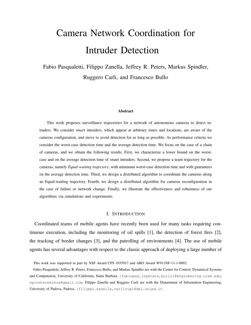
Fig. 1. This figure shows five cameras installed along a one dimensional open path. The field of view of each cameras is a
point on the path. Cameras coordinate their motion to detect smart moving intruders along the path.
static sensors, such as improved situation awareness and fast reconfigurability. In this paper we
address the challenging problem of scheduling the agents trajectories to optimize the performance
in persistent surveillance tasks.
Problem description. We consider a network of identical Pan-Tilt-Zoom (PTZ) cameras for
video surveillance, and we focus on the development of distributed and autonomous surveillance
strategies for the detection of moving intruders. We make combined assumptions on the envi-
ronment to be monitored, the cameras, and the intruders. We assume the environment to be one
dimensional, in the sense that it can be completely observed by a chain of cameras by using the
panning motion only (the perimeter surveillance problem is a special case of this framework).
We assume the cameras to be subject to physical constraints, such as limited field of view (f.o.v.)
and panning speed, and to be equipped with a low-level routine to detect intruders that fall within
their f.o.v.. We assume intruders to be smart, in the sense that they have access to the cameras
configuration at every time instant, and schedule their trajectory to avoid detection for as long
as possible. We also assume that intruders do not leave the environment once they have entered.
We propose cameras trajectories and control algorithms to minimize the worst case detection
time and the average detection time of smart intruders.
Related work. Of relevance to this work are the research areas of robotic patrolling and video
surveillance. In a typical robotic patrolling setup, the environment is represented by a graph on
which the agents motion is constrained, and the patrolling performance is given by the worst-
case detection time of static events. In [5], [6] an empirical evaluation of certain patrolling
heuristics is performed. In [4] and [2], an efficient and distributed solution to the (worst-case)
perimeter patrolling problem for robots with zero communication range is proposed. In [7] the
computational complexity of the patrolling problem is studied as a function of the environment
topology, and optimal strategies as well as constant-factor approximations are proposed. With
respect to these works, we consider smart intruders, as opposed to static ones, and we study
also the average detection time, as opposed to the worst case detection time only. In the context
of camera networks the perimeter patrolling problem is discussed in [8], [9], where distributed
algorithms are proposed for the cameras to partition a one-dimensional environment and to
coordinate along a trajectory with minimum worst-case detection time of static intruders. Graph
partitioning and intruder detection with minimum worst-case detection time for two-dimensional
camera networks is studied in [10]. We improve the results along this direction by showing that
the strategies proposed in [8], [9] generally fail at detecting smart intruders, and by studying
the average detection time of smart intruders. Complementary approaches based on numerical
analysis and game theory for the surveillance of two dimensional environments are discussed in
[11], [12]. Finally, a preliminary version of this work was presented in [13], [14].
In the context of video surveillance most approaches consider the case of static cameras,
where the surveillance problem reduces to an optimal sensor placement problem. In [15], this
sensor placement problem is considered in a static camera network with the goal of maximizing
the observability of a set of aggregate tasks that occur in a dynamic environment. In [16], a
similar problem is considered in a static camera network with the goal of visual tagging. In the
case of surveillance in active (PTZ) camera networks, [17] assumes the possibility to cover the
entire region at all times, and it considers the problem of coordinating camera motion using
a game-theoretic approach. With respect to this work, we do not make the assumption that
cameras can cover the whole region at all times, and we provide specific results for the case of
one-dimensional environment.
Contributions. The contributions of this work are as follows.
First, we mathematically formalize the concepts of cameras trajectory and smart intruder, and
we propose the trajectory design problem for video surveillance. We formalize the worst-case
detection time and average detection time criteria, and we characterize lower bounds on both
performance criteria.
Second, we propose the Equal-waiting cameras trajectory, which achieves minimum worst
case detection time, and constant factor optimal average detection time (under reasonable as-
sumptions). The Equal-waiting trajectory is easy to compute given a camera network, and it is
amenable to distributed implementation. In fact, we develop a distributed coordination algorithm
to steer the cameras along an equal-waiting trajectory. Our coordination algorithm converges
in finite time, which we characterize, and it requires only local communication and minimal
information to be implemented.
Third, we design a distributed reconfiguration algorithm for the cameras to react to failures and
to adapt to time-varying topologies. In particular, our reconfiguration algorithm takes advantage
of gossip communication to continuously partition the environment and, at the same time,
coordinate the motion of the cameras to optimize the detection performance.
Fourth and finally, we validate our findings through simulations and experiments. Through
simulations we validate our theoretical findings and algorithms for different configurations.
Analogously, our experiments validate our modeling framework and assumptions, and show
that our methods are robust to cameras failure, model uncertainties, and sensor noise.
Paper Organization. The remainder of the paper is organized as follows. Section II contains
our problem setup and some preliminary results. In Section III we present our main results, that
is, we propose and characterize the Equal-waiting trajectory, and we describe our distributed
coordination algorithm. In Section IV we detail our simulations and experiments. Section V
contains our algorithm for cameras reconfiguration. Finally, our conclusion and final remarks
are in Section VI.
II. PROBLEM SETUP AND PRELIMINARY RESULTS
In this section we describe the one-dimensional surveillance problem under consideration, and
we present some useful definitions and mathematical tools for its analysis.
A. Problem setting and notation
Consider a set of n ∈ N identical active cameras installed along a one dimensional open path
(boundary) Γ of length L (see Fig 1). For the ease of notation and without affecting generality,
we represent Γ with the segment [0, L], and we label the cameras in increasing order from c1
to cn according to their position on Γ. We make the following assumptions:
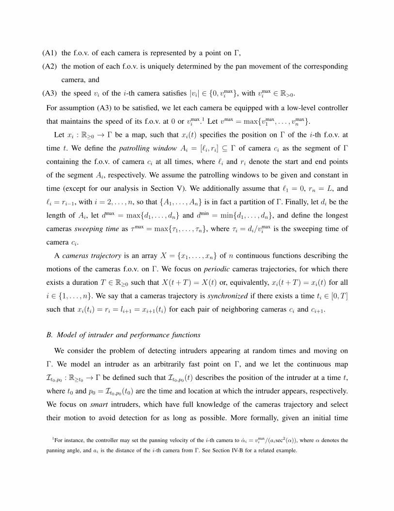
(A1) the f.o.v. of each camera is represented by a point on Γ,
(A2) the motion of each f.o.v. is uniquely determined by the pan movement of the corresponding
camera, and
(A3) the speed vi of the i-th camera satisfies |vi| ∈ 0, vmaxi , with vmax
i ∈ R>0.
For assumption (A3) to be satisfied, we let each camera be equipped with a low-level controller
that maintains the speed of its f.o.v. at 0 or vmaxi .1 Let vmax = maxvmax
1 , . . . , vmaxn .
Let xi : R≥0 → Γ be a map, such that xi(t) specifies the position on Γ of the i-th f.o.v. at
time t. We define the patrolling window Ai = [`i, ri] ⊆ Γ of camera ci as the segment of Γ
containing the f.o.v. of camera ci at all times, where `i and ri denote the start and end points
of the segment Ai, respectively. We assume the patrolling windows to be given and constant in
time (except for our analysis in Section V). We additionally assume that `1 = 0, rn = L, and
`i = ri−1, with i = 2, . . . , n, so that A1, . . . , An is in fact a partition of Γ. Finally, let di be the
length of Ai, let dmax = maxd1, . . . , dn and dmin = mind1, . . . , dn, and define the longest
cameras sweeping time as τmax = maxτ1, . . . , τn, where τi = di/vmaxi is the sweeping time of
camera ci.
A cameras trajectory is an array X = x1, . . . , xn of n continuous functions describing the
motions of the cameras f.o.v. on Γ. We focus on periodic cameras trajectories, for which there
exists a duration T ∈ R≥0 such that X(t+ T ) = X(t) or, equivalently, xi(t+ T ) = xi(t) for all
i ∈ 1, . . . , n. We say that a cameras trajectory is synchronized if there exists a time ti ∈ [0, T ]
such that xi(ti) = ri = li+1 = xi+1(ti) for each pair of neighboring cameras ci and ci+1.
B. Model of intruder and performance functions
We consider the problem of detecting intruders appearing at random times and moving on
Γ. We model an intruder as an arbitrarily fast point on Γ, and we let the continuous map
It0,p0 : R≥t0 → Γ be defined such that It0,p0(t) describes the position of the intruder at a time t,
where t0 and p0 = It0,p0(t0) are the time and location at which the intruder appears, respectively.
We focus on smart intruders, which have full knowledge of the cameras trajectory and select
their motion to avoid detection for as long as possible. More formally, given an initial time
1For instance, the controller may set the panning velocity of the i-th camera to αi = vmaxi /(aisec2(α)), where α denotes the
panning angle, and ai is the distance of the i-th camera from Γ. See Section IV-B for a related example.
dis
tance
time
d1
d2
d3
x1(t)
x2(t)
x3(t)e2
e1
!
0
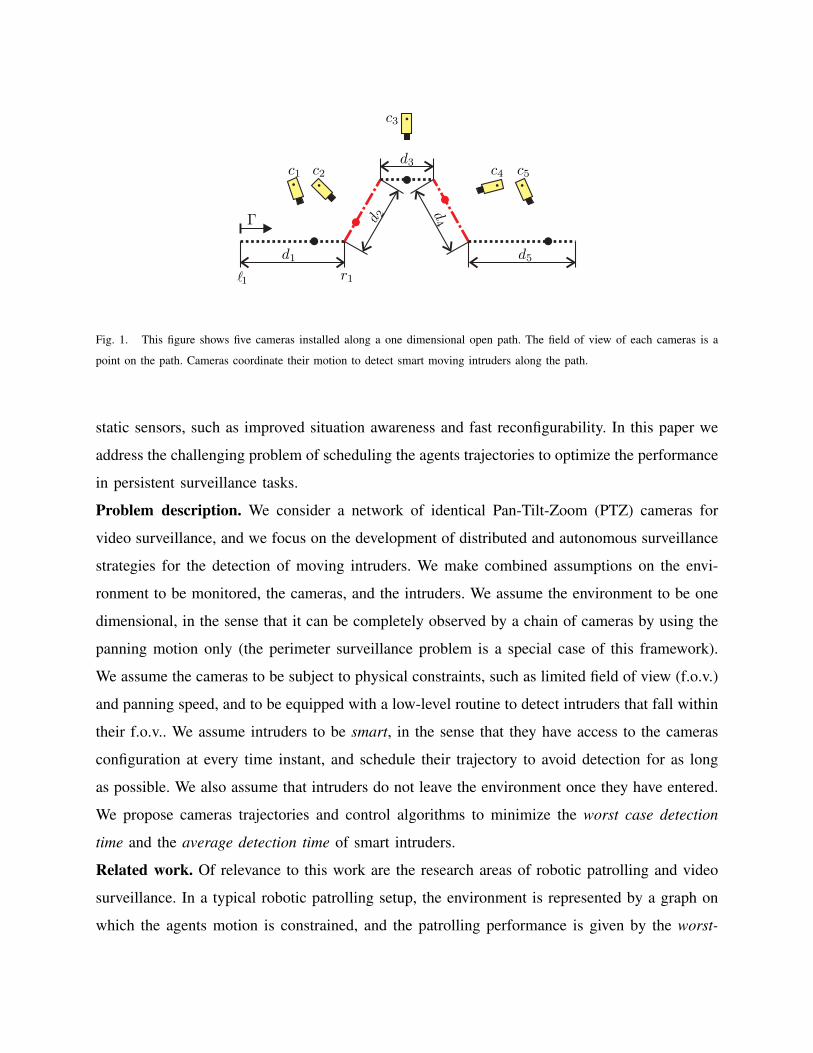
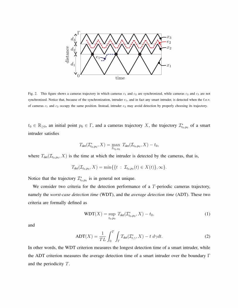
Fig. 2. This figure shows a cameras trajectory in which cameras c1 and c2 are synchronized, while cameras c2 and c3 are not
synchronized. Notice that, because of the synchronization, intruder e1, and in fact any smart intruder, is detected when the f.o.v.
of cameras c1 and c2 occupy the same position. Instead, intruder e2 may avoid detection by properly choosing its trajectory.
t0 ∈ R≥0, an initial point p0 ∈ Γ, and a cameras trajectory X , the trajectory I∗t0,p0 of a smart
intruder satisfies
Tdet(I∗t0,p0 , X) = maxIt0,p0
Tdet(It0,p0 , X)− t0,
where Tdet(It0,p0 , X) is the time at which the intruder is detected by the cameras, that is,
Tdet(It0,p0 , X) = mint : It0,p0(t) ∈ X(t),∞.
Notice that the trajectory I∗t0,p0 is in general not unique.
We consider two criteria for the detection performance of a T -periodic cameras trajectory,
namely the worst-case detection time (WDT), and the average detection time (ADT). These two
criteria are formally defined as
WDT(X) = supt0,p0
Tdet(I∗t0,p0 , X)− t0, (1)
and
ADT(X) =1
TL
∫ T
0
∫Γ
Tdet(I∗t,γ, X)− t dγdt. (2)
In other words, the WDT criterion measures the longest detection time of a smart intruder, while
the ADT criterion measures the average detection time of a smart intruder over the boundary Γ
and the periodicity T .
The worst case detection time criterion for static intruders, namely WDTs, is defined in [18]
as
WDTs(X) = supt0,p0
t− t0 : t ≥ t0, p0 ∈ X(t), (3)
and it corresponds to the longest time for the cameras to detect a static intruder, or simply event,
along Γ. We next informally discuss the relation between WDT and WDTs, and we refer the
reader to [7], [8], [18] for a proof of these results. Let
WDT∗ = minX
WDT(X), and WDTs∗ = minX
WDTs(X).
Clearly, WDT(X) ≥ WDTs(X) for every cameras trajectory X . For instance, as shown by the
example in Fig. 2, if a cameras trajectory X is not synchronized and yet it covers every location
of Γ, then WDTs(X) < ∞ and WDT(X) = ∞. Additionally, because the patrolling windows
define a partition of Γ, it can be easily verified that the static worst case detection time satisfies
WDTs∗ = 2τmax,
and that any 2τmax-periodic cameras trajectory achieves minimum static worst-case detection
time. Similarly, any synchronized 2τmax-periodic cameras trajectory X satisfies (see Fig. 2)
WDT(X) = 2τmax. (4)
Thus, any synchronized 2τmax-periodic cameras trajectory achieves minimum worst-case detec-
tion time (WDT and WDTs). This discussion motivates us to restrict our attention to periodic
and synchronized cameras trajectories.
Problem 1 (Design of cameras trajectories) Consider an open path partitioned among a set
of n cameras, and let τmax be the longest cameras sweeping time. Design a cameras trajectory
X∗ satisfying
ADT(X∗) = ADT∗ = minX∈Ω
ADT(X),
where Ω is the set of all synchronized 2τmax-periodic cameras trajectories.
Remark 1 (Optimal patrolling windows) We assume that the patrolling windows are given and
form a partition of the path Γ. With these assumptions, the worst-case detection time satisfies
WDT∗ ≥ WDTs∗ ≥ 2τmax, and any synchronized 2τmax-periodic cameras trajectory achieves
the lower bound.
If the patrolling windows are not given but are still required to be a partition of Γ, then
the longest cameras sweeping time, and hence the worst-case detection performance, can be
minimized by solving a min-max partitioning problem [7], [18], [14]. We will discuss this
partitioning problem in Section V, where we develop an algorithm to simultaneously partition
the boundary and coordinate the motion of the cameras.
If the patrolling windows are not required to be a partition of Γ, then WDTs∗ may be smaller
than 2τ ∗. We refer the interested reader to [19, Conjecture 1] and [20].
A second focus of this paper is the design of distributed coordination algorithms for the
cameras to converge to a desired trajectory. We consider a distributed scenario in which cameras
ci and cj are allowed to communicate at time t only if |j − i| = 1 (neighboring cameras) and
xi(t) = xj(t). Although conservative, this assumption allows us to design algorithms imple-
mentable with many low-cost communication devices; see Section IV-B. Notice that additional
communications cannot decrease the performance of our algorithm.
Problem 2 (Distributed coordination) For a set of n cameras on a one-dimensional open path,
design a distributed algorithm to coordinate the cameras along a trajectory with minimum
average detection time of smart intruders.
III. EQUAL-WAITING CAMERAS TRAJECTORY AND COORDINATION ALGORITHM
In this section we present our results for Problems 1 and 2. In particular, we propose a
cameras trajectory with performance guarantees for the average detection time, and a distributed
algorithm for the cameras to converge to such a trajectory. We remark that in some cases an
exact solution to Problem 1 can be computed through standard optimization techniques [21].
Such computation, however, is not scalable with the number of cameras, and it is not amenable
to distributed implementation. Instead, our approximate solution is valid for every number of
cameras and environment configuration, is extremely simple and efficient to compute, and its
performance is shown to be within a bound of the optimum. The cameras trajectory that we
propose can informally be described as follows:
d1
d2 = dmax
d3
d4
T = 2τmax
1 = 0
2 = r1
3 = r2
4 = r3
r4 = Γ
dis
tance
time
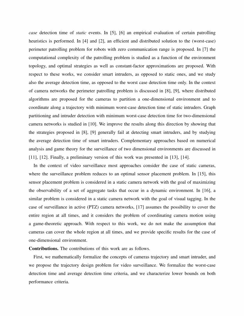
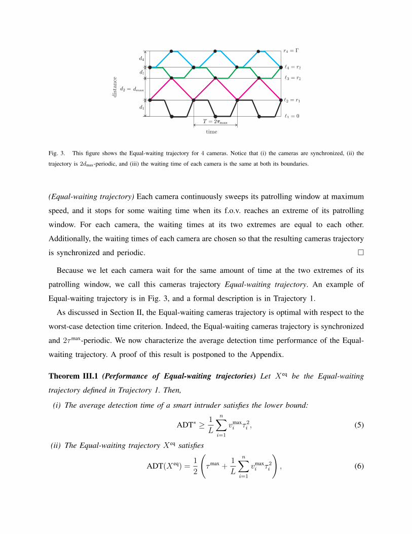
Fig. 3. This figure shows the Equal-waiting trajectory for 4 cameras. Notice that (i) the cameras are synchronized, (ii) the
trajectory is 2dmax-periodic, and (iii) the waiting time of each camera is the same at both its boundaries.
(Equal-waiting trajectory) Each camera continuously sweeps its patrolling window at maximum
speed, and it stops for some waiting time when its f.o.v. reaches an extreme of its patrolling
window. For each camera, the waiting times at its two extremes are equal to each other.
Additionally, the waiting times of each camera are chosen so that the resulting cameras trajectory
is synchronized and periodic.
Because we let each camera wait for the same amount of time at the two extremes of its
patrolling window, we call this cameras trajectory Equal-waiting trajectory. An example of
Equal-waiting trajectory is in Fig. 3, and a formal description is in Trajectory 1.
As discussed in Section II, the Equal-waiting cameras trajectory is optimal with respect to the
worst-case detection time criterion. Indeed, the Equal-waiting cameras trajectory is synchronized
and 2τmax-periodic. We now characterize the average detection time performance of the Equal-
waiting trajectory. A proof of this result is postponed to the Appendix.
Theorem III.1 (Performance of Equal-waiting trajectories) Let Xeq be the Equal-waiting
trajectory defined in Trajectory 1. Then,
(i) The average detection time of a smart intruder satisfies the lower bound:
ADT∗ ≥ 1
L
n∑i=1
vmaxi τ 2
i , (5)
(ii) The Equal-waiting trajectory Xeq satisfies
ADT(Xeq) =1
2
(τmax +
1
L
n∑i=1
vmaxi τ 2
i
), (6)
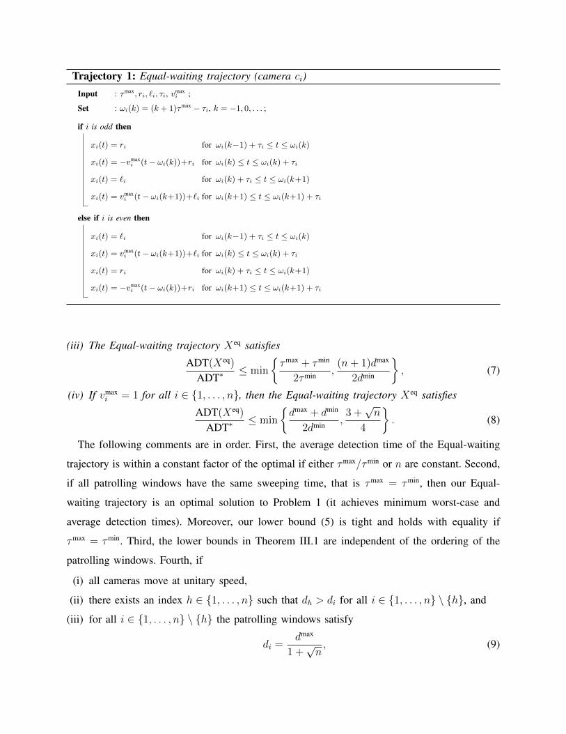
Trajectory 1: Equal-waiting trajectory (camera ci)
Input : τmax, ri, `i, τi, vmaxi ;
Set : ωi(k) = (k + 1)τmax − τi, k = −1, 0, . . . ;
if i is odd then
xi(t) = ri for ωi(k−1) + τi ≤ t ≤ ωi(k)
xi(t) = −vmaxi (t− ωi(k))+ri for ωi(k) ≤ t ≤ ωi(k) + τi
xi(t) = `i for ωi(k) + τi ≤ t ≤ ωi(k+1)
xi(t) = vmaxi (t− ωi(k+1))+`i for ωi(k+1) ≤ t ≤ ωi(k+1) + τi
else if i is even then
xi(t) = `i for ωi(k−1) + τi ≤ t ≤ ωi(k)
xi(t) = vmaxi (t− ωi(k+1))+`i for ωi(k) ≤ t ≤ ωi(k) + τi
xi(t) = ri for ωi(k) + τi ≤ t ≤ ωi(k+1)
xi(t) = −vmaxi (t− ωi(k))+ri for ωi(k+1) ≤ t ≤ ωi(k+1) + τi
(iii) The Equal-waiting trajectory Xeq satisfies
ADT(Xeq)
ADT∗≤ min
τmax + τmin
2τmin ,(n+ 1)dmax
2dmin
, (7)
(iv) If vmaxi = 1 for all i ∈ 1, . . . , n, then the Equal-waiting trajectory Xeq satisfies
ADT(Xeq)
ADT∗≤ min
dmax + dmin
2dmin ,3 +√n
4
. (8)
The following comments are in order. First, the average detection time of the Equal-waiting
trajectory is within a constant factor of the optimal if either τmax/τmin or n are constant. Second,
if all patrolling windows have the same sweeping time, that is τmax = τmin, then our Equal-
waiting trajectory is an optimal solution to Problem 1 (it achieves minimum worst-case and
average detection times). Moreover, our lower bound (5) is tight and holds with equality if
τmax = τmin. Third, the lower bounds in Theorem III.1 are independent of the ordering of the
patrolling windows. Fourth, if
(i) all cameras move at unitary speed,
(ii) there exists an index h ∈ 1, . . . , n such that dh > di for all i ∈ 1, . . . , n \ h, and
(iii) for all i ∈ 1, . . . , n \ h the patrolling windows satisfy
di =dmax
1 +√n, (9)
then (see the proof of Theorem III.1 and Fig. 4(b))
ADT(Xeq)
ADT∗=
3 +√n
4. (10)
Fifth and finally, different cameras speeds can be taken into account in our bound (8). In fact,
if vmaxi /vmax
j ≤ C for all i, j ∈ 1, . . . , n and for some C ∈ R, then (see the proof of Theorem
III.1)
ADT(Xeq)
ADT∗≤ min
C(dmax + dmin
)2dmin ,
2 + C (1 +√n)
4
.
We now design a distributed feedback algorithm that steers the cameras towards an Equal-
waiting trajectory. Our coordination algorithm is informally described as follows:
(Distributed coordination) Camera ci moves to `i and, if i > 1, it waits until the f.o.v. of its
left neighboring camera ci−1 occupies the same position. Then, camera ci stops as specified in
Trajectory 1, and finally move to ri. Camera c1 (resp. cn) moves to r2 (resp. `n−1) as soon as
its f.o.v. arrives at `1 (resp. rn).
Our coordination algorithm is formally described in Algorithm 2, where for convenience we
set x0(t) = `1 and xn+1(t) = rn at all times.
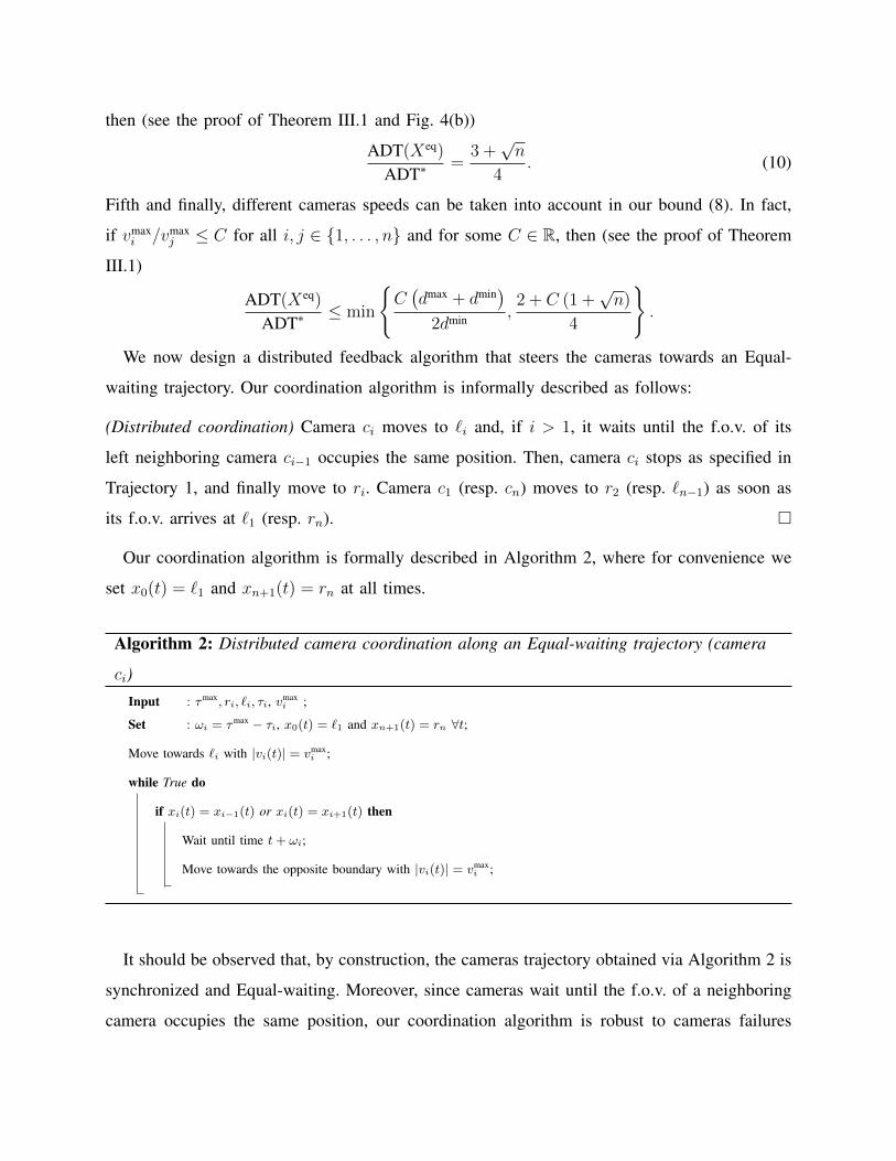
Algorithm 2: Distributed camera coordination along an Equal-waiting trajectory (camera
ci)
Input : τmax, ri, `i, τi, vmaxi ;
Set : ωi = τmax − τi, x0(t) = `1 and xn+1(t) = rn ∀t;
Move towards `i with |vi(t)| = vmaxi ;
while True do
if xi(t) = xi−1(t) or xi(t) = xi+1(t) then
Wait until time t+ ωi;
Move towards the opposite boundary with |vi(t)| = vmaxi ;
It should be observed that, by construction, the cameras trajectory obtained via Algorithm 2 is
synchronized and Equal-waiting. Moreover, since cameras wait until the f.o.v. of a neighboring
camera occupies the same position, our coordination algorithm is robust to cameras failures
and motion uncertainties. A related example is in Section IV-A. Regarding the implementation
of Algorithm 2, notice that each camera is required to know the endpoints of its patrolling
window, its sweeping time and the maximum sweeping time in the network, and to be able to
communicate with neighboring cameras. The following theorem characterizes the convergence
properties of Algorithm 2, where we write X(t ≥ t) to denote the restriction of the trajectory
X(t) to the interval t ∈ [t,∞).
Theorem III.2 (Convergence of Algorithm 2) For a set of n cameras with sweeping times
τ1, . . . , τn, let X(t) be the cameras trajectory generated by Algorithm 2. Then, X(t ≥ nτmax) is
an Equal-waiting trajectory.
Proof: Notice that the f.o.v. of camera c1 coincides with the f.o.v. of camera c2 within
time max2τ1, τ2 ≤ 2τmax. Then, the f.o.v. of camera ci coincides with the f.o.v. of camera
ci+1 within time (i+ 1)τmax. Hence, within time nτmax the cameras trajectory coincides with an
Equal-waiting trajectory in Trajectory 1. The claimed statement follows.
IV. SIMULATIONS AND EXPERIMENTS
In this section we report the results of our simulation studies and experiments. Besides
validating our theory, these results show that our models are accurate, that our algorithms can
be implemented on real hardware, and that our algorithms are robust to sensor noise and model
uncertainties.
A. Simulations
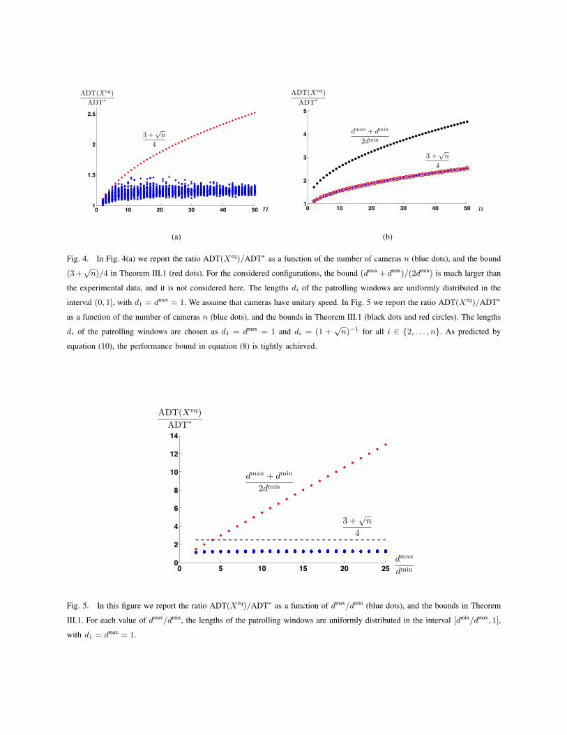
Three simulation studies are presented in this section. For our first simulation study, we let the
number of cameras n vary from 2 to 50. For each value of n, we generate 50 sets of patrolling
window with lengths d1, . . . , dn, where d1 = dmax = 1 m, and di is uniformly distributed within
the interval (0, 1] m , for all i ∈ 2, . . . , n. For each configuration we let vmaxi = 1 m/s for all
cameras, we design the Equal-waiting trajectory Xeq, and we evaluate the cost ADT(Xeq) and
the lower bound ADT∗ from equation (5). We report the result of this study in Fig. 4(a). Notice
that, when the number of cameras is and the lengths of the patrolling windows are uniformly
distributed, the bound in (8) is conservative. On the other hand, if the lengths of the patrolling
windows are chosen as in (9), then the bound in (8) is tightly achieved (Fig. 4(b)).
0 10 20 30 40 501
1.5
2
2.5
ADT(Xeq)
ADT
n
3 +p
n
4
(a)
0 10 20 30 40 501
2
3
4
5
ADT(Xeq)
ADT
dmax + dmin
2dmin
3 +p
n
4
n
(b)
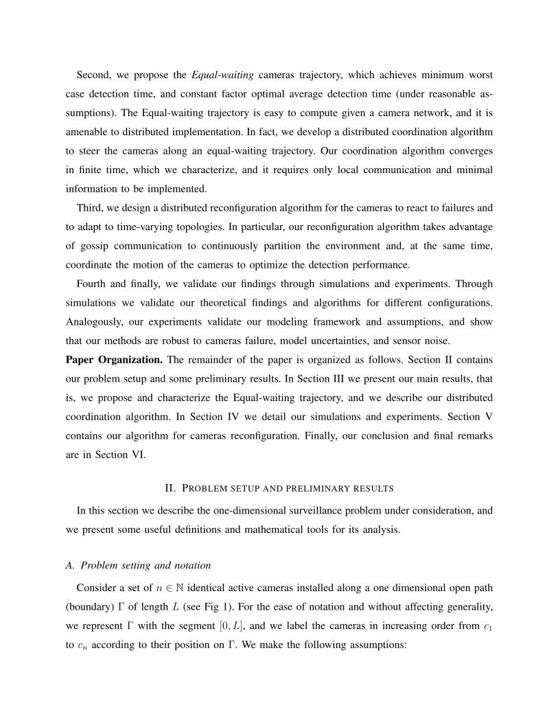
Fig. 4. In Fig. 4(a) we report the ratio ADT(Xeq)/ADT∗ as a function of the number of cameras n (blue dots), and the bound
(3 +√n)/4 in Theorem III.1 (red dots). For the considered configurations, the bound (dmax +dmin)/(2dmin) is much larger than
the experimental data, and it is not considered here. The lengths di of the patrolling windows are uniformly distributed in the
interval (0, 1], with d1 = dmax = 1. We assume that cameras have unitary speed. In Fig. 5 we report the ratio ADT(Xeq)/ADT∗
as a function of the number of cameras n (blue dots), and the bounds in Theorem III.1 (black dots and red circles). The lengths
di of the patrolling windows are chosen as d1 = dmax = 1 and di = (1 +√n)−1 for all i ∈ 2, . . . , n. As predicted by
equation (10), the performance bound in equation (8) is tightly achieved.
0 5 10 15 20 250
2
4
6
8
10
12
14
ADT(Xeq)
ADT
dmax
dmin
dmax + dmin
2dmin
3 +p
n
4
Fig. 5. In this figure we report the ratio ADT(Xeq)/ADT∗ as a function of dmax/dmin (blue dots), and the bounds in Theorem
III.1. For each value of dmax/dmin, the lengths of the patrolling windows are uniformly distributed in the interval [dmin/dmax, 1],
with d1 = dmax = 1.
0 100 200 300 400 500 600 700 800 900 10000
1
2
3
4
5
6
Time
Pat
h
Simulation of n=4 w/ initialization phase and temporary camera failure
tinitialization noisefailure
0 100 200 300 400 500 600 700 800 900 10000
1
2
3
4
5
6
dis
tance
(m
)
time (s)
x1
x2
x3
x4
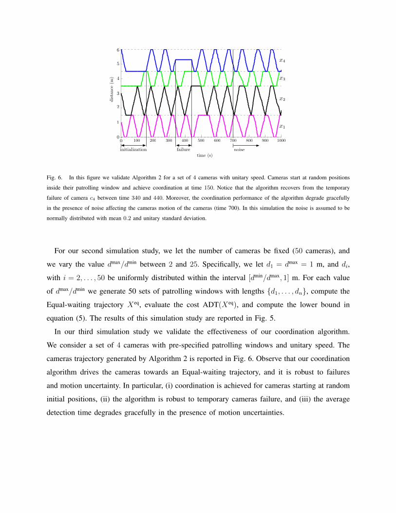
Fig. 6. In this figure we validate Algorithm 2 for a set of 4 cameras with unitary speed. Cameras start at random positions
inside their patrolling window and achieve coordination at time 150. Notice that the algorithm recovers from the temporary
failure of camera c4 between time 340 and 440. Moreover, the coordination performance of the algorithm degrade gracefully
in the presence of noise affecting the cameras motion of the cameras (time 700). In this simulation the noise is assumed to be
normally distributed with mean 0.2 and unitary standard deviation.
For our second simulation study, we let the number of cameras be fixed (50 cameras), and
we vary the value dmax/dmin between 2 and 25. Specifically, we let d1 = dmax = 1 m, and di,
with i = 2, . . . , 50 be uniformly distributed within the interval [dmin/dmax, 1] m. For each value
of dmax/dmin we generate 50 sets of patrolling windows with lengths d1, . . . , dn, compute the
Equal-waiting trajectory Xeq, evaluate the cost ADT(Xeq), and compute the lower bound in
equation (5). The results of this simulation study are reported in Fig. 5.
In our third simulation study we validate the effectiveness of our coordination algorithm.
We consider a set of 4 cameras with pre-specified patrolling windows and unitary speed. The
cameras trajectory generated by Algorithm 2 is reported in Fig. 6. Observe that our coordination
algorithm drives the cameras towards an Equal-waiting trajectory, and it is robust to failures
and motion uncertainty. In particular, (i) coordination is achieved for cameras starting at random
initial positions, (ii) the algorithm is robust to temporary cameras failure, and (iii) the average
detection time degrades gracefully in the presence of motion uncertainties.
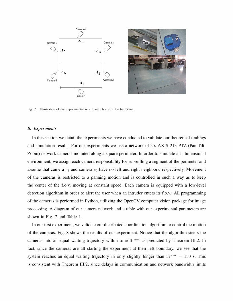
Fig. 7. Illustration of the experimental set-up and photos of the hardware.
B. Experiments
In this section we detail the experiments we have conducted to validate our theoretical findings
and simulation results. For our experiments we use a network of six AXIS 213 PTZ (Pan-Tilt-
Zoom) network cameras mounted along a square perimeter. In order to simulate a 1-dimensional
environment, we assign each camera responsibility for surveilling a segment of the perimeter and
assume that camera c1 and camera c6 have no left and right neighbors, respectively. Movement
of the cameras is restricted to a panning motion and is controlled in such a way as to keep
the center of the f.o.v. moving at constant speed. Each camera is equipped with a low-level
detection algorithm in order to alert the user when an intruder enters its f.o.v.. All programming
of the cameras is performed in Python, utilizing the OpenCV computer vision package for image
processing. A diagram of our camera network and a table with our experimental parameters are
shown in Fig. 7 and Table I.
In our first experiment, we validate our distributed coordination algorithm to control the motion
of the cameras. Fig. 8 shows the results of our experiment. Notice that the algorithm steers the
cameras into an equal waiting trajectory within time 6τmax as predicted by Theorem III.2. In
fact, since the cameras are all starting the experiment at their left boundary, we see that the
system reaches an equal waiting trajectory in only slightly longer than 5τmax = 150 s. This
is consistent with Theorem III.2, since delays in communication and network bandwidth limits
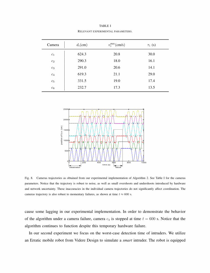
TABLE I
RELEVANT EXPERIMENTAL PARAMETERS.
Camera di(cm) vmaxi (cm/s) τi (s)
c1 624.3 20.8 30.0
c2 290.3 18.0 16.1
c3 291.0 20.6 14.1
c4 619.3 21.1 29.0
c5 331.5 19.0 17.4
c6 232.7 17.3 13.5
Fig. 8. Cameras trajectories as obtained from our experimental implementation of Algorithm 2. See Table I for the cameras
parameters. Notice that the trajectory is robust to noise, as well as small overshoots and undershoots introduced by hardware
and network uncertainty. These inaccuracies in the individual camera trajectories do not significantly affect coordination. The
cameras trajectory is also robust to momentary failures, as shown at time t ≈ 600 s.
cause some lagging in our experimental implementation. In order to demonstrate the behavior
of the algorithm under a camera failure, camera c4 is stopped at time t = 600 s. Notice that the
algorithm continues to function despite this temporary hardware failure.
In our second experiment we focus on the worst-case detection time of intruders. We utilize
an Erratic mobile robot from Videre Design to simulate a smart intruder. The robot is equipped
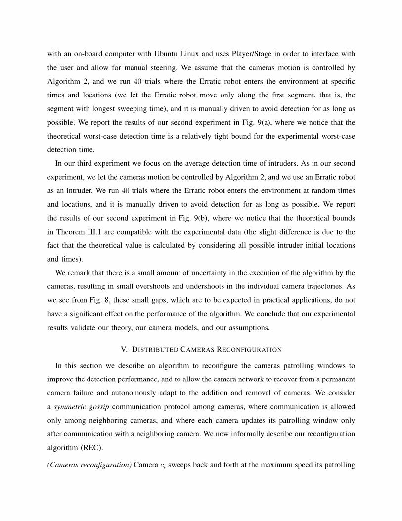
with an on-board computer with Ubuntu Linux and uses Player/Stage in order to interface with
the user and allow for manual steering. We assume that the cameras motion is controlled by
Algorithm 2, and we run 40 trials where the Erratic robot enters the environment at specific
times and locations (we let the Erratic robot move only along the first segment, that is, the
segment with longest sweeping time), and it is manually driven to avoid detection for as long as
possible. We report the results of our second experiment in Fig. 9(a), where we notice that the
theoretical worst-case detection time is a relatively tight bound for the experimental worst-case
detection time.
In our third experiment we focus on the average detection time of intruders. As in our second
experiment, we let the cameras motion be controlled by Algorithm 2, and we use an Erratic robot
as an intruder. We run 40 trials where the Erratic robot enters the environment at random times
and locations, and it is manually driven to avoid detection for as long as possible. We report
the results of our second experiment in Fig. 9(b), where we notice that the theoretical bounds
in Theorem III.1 are compatible with the experimental data (the slight difference is due to the
fact that the theoretical value is calculated by considering all possible intruder initial locations
and times).
We remark that there is a small amount of uncertainty in the execution of the algorithm by the
cameras, resulting in small overshoots and undershoots in the individual camera trajectories. As
we see from Fig. 8, these small gaps, which are to be expected in practical applications, do not
have a significant effect on the performance of the algorithm. We conclude that our experimental
results validate our theory, our camera models, and our assumptions.
V. DISTRIBUTED CAMERAS RECONFIGURATION
In this section we describe an algorithm to reconfigure the cameras patrolling windows to
improve the detection performance, and to allow the camera network to recover from a permanent
camera failure and autonomously adapt to the addition and removal of cameras. We consider
a symmetric gossip communication protocol among cameras, where communication is allowed
only among neighboring cameras, and where each camera updates its patrolling window only
after communication with a neighboring camera. We now informally describe our reconfiguration
algorithm (REC).
(Cameras reconfiguration) Camera ci sweeps back and forth at the maximum speed its patrolling
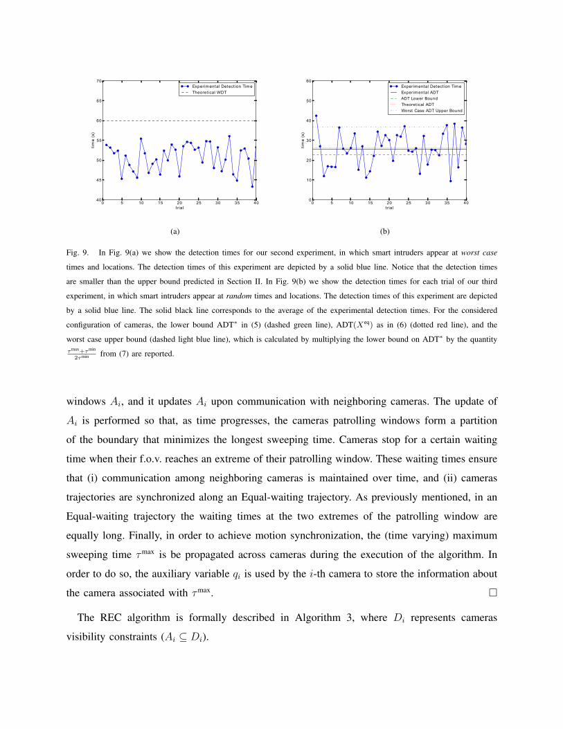
(a) (b)
Fig. 9. In Fig. 9(a) we show the detection times for our second experiment, in which smart intruders appear at worst case
times and locations. The detection times of this experiment are depicted by a solid blue line. Notice that the detection times
are smaller than the upper bound predicted in Section II. In Fig. 9(b) we show the detection times for each trial of our third
experiment, in which smart intruders appear at random times and locations. The detection times of this experiment are depicted
by a solid blue line. The solid black line corresponds to the average of the experimental detection times. For the considered
configuration of cameras, the lower bound ADT∗ in (5) (dashed green line), ADT(Xeq) as in (6) (dotted red line), and the
worst case upper bound (dashed light blue line), which is calculated by multiplying the lower bound on ADT∗ by the quantityτmax+τmin
2τmin from (7) are reported.
windows Ai, and it updates Ai upon communication with neighboring cameras. The update of
Ai is performed so that, as time progresses, the cameras patrolling windows form a partition
of the boundary that minimizes the longest sweeping time. Cameras stop for a certain waiting
time when their f.o.v. reaches an extreme of their patrolling window. These waiting times ensure
that (i) communication among neighboring cameras is maintained over time, and (ii) cameras
trajectories are synchronized along an Equal-waiting trajectory. As previously mentioned, in an
Equal-waiting trajectory the waiting times at the two extremes of the patrolling window are
equally long. Finally, in order to achieve motion synchronization, the (time varying) maximum
sweeping time τmax is be propagated across cameras during the execution of the algorithm. In
order to do so, the auxiliary variable qi is used by the i-th camera to store the information about
the camera associated with τmax.
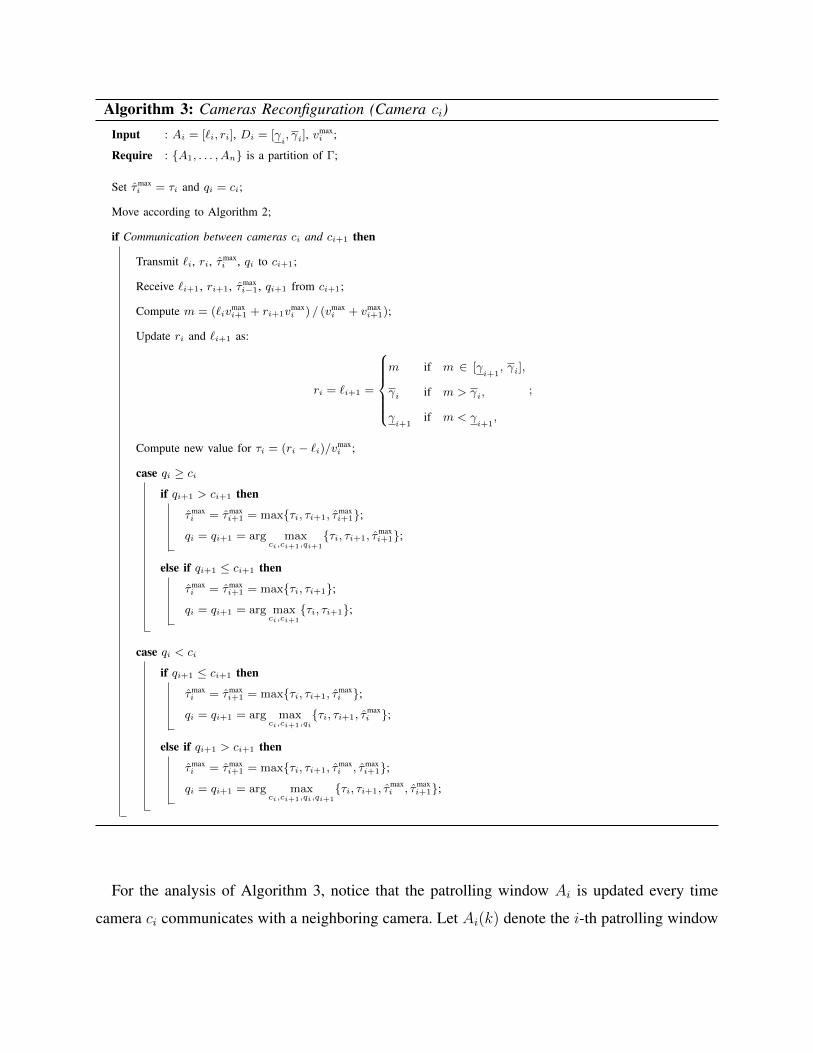
The REC algorithm is formally described in Algorithm 3, where Di represents cameras
visibility constraints (Ai ⊆ Di).
Algorithm 3: Cameras Reconfiguration (Camera ci)
Input : Ai = [`i, ri], Di = [γi, γi], v
maxi ;
Require : A1, . . . , An is a partition of Γ;
Set τmaxi = τi and qi = ci;
Move according to Algorithm 2;
if Communication between cameras ci and ci+1 then
Transmit `i, ri, τmaxi , qi to ci+1;
Receive `i+1, ri+1, τmaxi−1, qi+1 from ci+1;
Compute m = (`ivmaxi+1 + ri+1v
maxi ) / (vmax
i + vmaxi+1);
Update ri and `i+1 as:
ri = `i+1 =
m if m ∈ [γ
i+1, γi],
γi if m > γi,
γi+1
if m < γi+1
,
;
Compute new value for τi = (ri − `i)/vmaxi ;
case qi ≥ ciif qi+1 > ci+1 then
τmaxi = τmax
i+1 = maxτi, τi+1, τmaxi+1;
qi = qi+1 = arg maxci,ci+1,qi+1
τi, τi+1, τmaxi+1;
else if qi+1 ≤ ci+1 then
τmaxi = τmax
i+1 = maxτi, τi+1;
qi = qi+1 = arg maxci,ci+1
τi, τi+1;
case qi < ci
if qi+1 ≤ ci+1 then
τmaxi = τmax
i+1 = maxτi, τi+1, τmaxi ;
qi = qi+1 = arg maxci,ci+1,qi
τi, τi+1, τmaxi ;
else if qi+1 > ci+1 then
τmaxi = τmax
i+1 = maxτi, τi+1, τmaxi , τmax
i+1;
qi = qi+1 = arg maxci,ci+1,qi,qi+1
τi, τi+1, τmaxi , τmax
i+1;
For the analysis of Algorithm 3, notice that the patrolling window Ai is updated every time
camera ci communicates with a neighboring camera. Let Ai(k) denote the i-th patrolling window
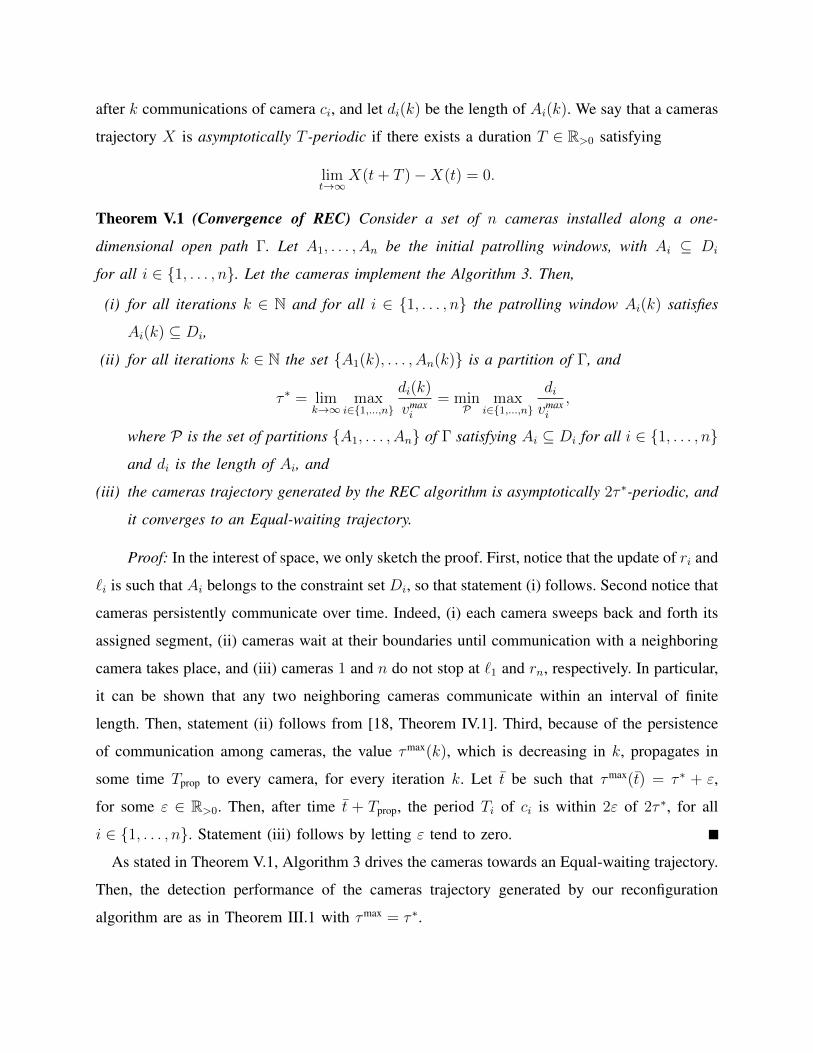
after k communications of camera ci, and let di(k) be the length of Ai(k). We say that a cameras
trajectory X is asymptotically T -periodic if there exists a duration T ∈ R>0 satisfying
limt→∞
X(t+ T )−X(t) = 0.
Theorem V.1 (Convergence of REC) Consider a set of n cameras installed along a one-
dimensional open path Γ. Let A1, . . . , An be the initial patrolling windows, with Ai ⊆ Di
for all i ∈ 1, . . . , n. Let the cameras implement the Algorithm 3. Then,
(i) for all iterations k ∈ N and for all i ∈ 1, . . . , n the patrolling window Ai(k) satisfies
Ai(k) ⊆ Di,
(ii) for all iterations k ∈ N the set A1(k), . . . , An(k) is a partition of Γ, and
τ ∗ = limk→∞
maxi∈1,...,n
di(k)
vmaxi
= minP
maxi∈1,...,n
divmaxi
,
where P is the set of partitions A1, . . . , An of Γ satisfying Ai ⊆ Di for all i ∈ 1, . . . , nand di is the length of Ai, and
(iii) the cameras trajectory generated by the REC algorithm is asymptotically 2τ ∗-periodic, and
it converges to an Equal-waiting trajectory.
Proof: In the interest of space, we only sketch the proof. First, notice that the update of ri and
`i is such that Ai belongs to the constraint set Di, so that statement (i) follows. Second notice that
cameras persistently communicate over time. Indeed, (i) each camera sweeps back and forth its
assigned segment, (ii) cameras wait at their boundaries until communication with a neighboring
camera takes place, and (iii) cameras 1 and n do not stop at `1 and rn, respectively. In particular,
it can be shown that any two neighboring cameras communicate within an interval of finite
length. Then, statement (ii) follows from [18, Theorem IV.1]. Third, because of the persistence
of communication among cameras, the value τmax(k), which is decreasing in k, propagates in
some time Tprop to every camera, for every iteration k. Let t be such that τmax(t) = τ ∗ + ε,
for some ε ∈ R>0. Then, after time t + Tprop, the period Ti of ci is within 2ε of 2τ ∗, for all
i ∈ 1, . . . , n. Statement (iii) follows by letting ε tend to zero.
As stated in Theorem V.1, Algorithm 3 drives the cameras towards an Equal-waiting trajectory.
Then, the detection performance of the cameras trajectory generated by our reconfiguration
algorithm are as in Theorem III.1 with τmax = τ ∗.
0 50 100 150 2000
5
10
15
20
time (s)
camerastrajectories
(m)
(a)
0 50 100 150 2003
4
5
6
7
8
9
!max,itrajectories
(s)
time (s)
(b)
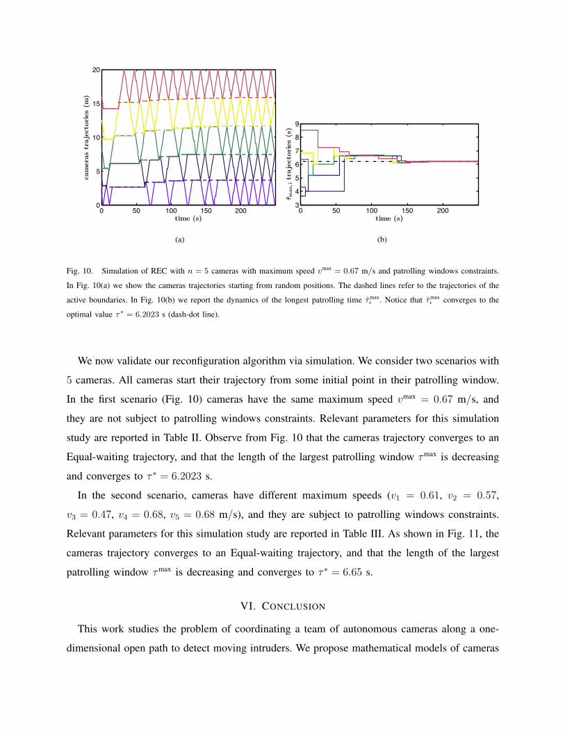
Fig. 10. Simulation of REC with n = 5 cameras with maximum speed vmax = 0.67 m/s and patrolling windows constraints.
In Fig. 10(a) we show the cameras trajectories starting from random positions. The dashed lines refer to the trajectories of the
active boundaries. In Fig. 10(b) we report the dynamics of the longest patrolling time τmaxi . Notice that τmax
i converges to the
optimal value τ∗ = 6.2023 s (dash-dot line).
We now validate our reconfiguration algorithm via simulation. We consider two scenarios with
5 cameras. All cameras start their trajectory from some initial point in their patrolling window.
In the first scenario (Fig. 10) cameras have the same maximum speed vmax = 0.67 m/s, and
they are not subject to patrolling windows constraints. Relevant parameters for this simulation
study are reported in Table II. Observe from Fig. 10 that the cameras trajectory converges to an
Equal-waiting trajectory, and that the length of the largest patrolling window τmax is decreasing
and converges to τ ∗ = 6.2023 s.
In the second scenario, cameras have different maximum speeds (v1 = 0.61, v2 = 0.57,
v3 = 0.47, v4 = 0.68, v5 = 0.68 m/s), and they are subject to patrolling windows constraints.
Relevant parameters for this simulation study are reported in Table III. As shown in Fig. 11, the
cameras trajectory converges to an Equal-waiting trajectory, and that the length of the largest
patrolling window τmax is decreasing and converges to τ ∗ = 6.65 s.
VI. CONCLUSION
This work studies the problem of coordinating a team of autonomous cameras along a one-
dimensional open path to detect moving intruders. We propose mathematical models of cameras
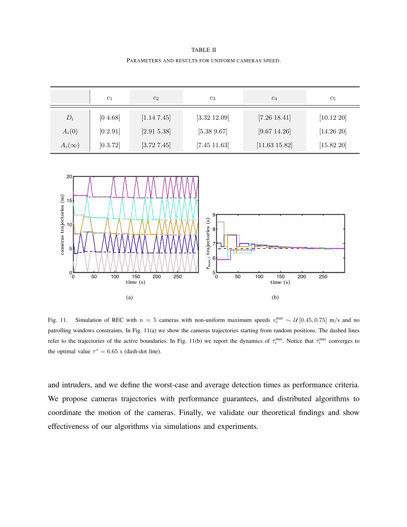
TABLE II
PARAMETERS AND RESULTS FOR UNIFORM CAMERAS SPEED.
c1 c2 c3 c4 c5
Di [0 4.68] [1.14 7.45] [3.32 12.09] [7.26 18.41] [10.12 20]
Ai(0) [0 2.91] [2.91 5.38] [5.38 9.67] [9.67 14.26] [14.26 20]
Ai(∞) [0 3.72] [3.72 7.45] [7.45 11.63] [11.63 15.82] [15.82 20]
0 50 100 150 200 2500
5
10
15
20
time (s)
camerastrajectories
(m)
(a)
0 50 100 150 200 2505
6
7
8
9!max,itrajectories
(s)
time (s)
(b)
Fig. 11. Simulation of REC with n = 5 cameras with non-uniform maximum speeds vmaxi ∼ U [0.45, 0.75] m/s and no
patrolling windows constraints. In Fig. 11(a) we show the cameras trajectories starting from random positions. The dashed lines
refer to the trajectories of the active boundaries. In Fig. 11(b) we report the dynamics of τmaxi . Notice that τmax
i converges to
the optimal value τ∗ = 6.65 s (dash-dot line).
and intruders, and we define the worst-case and average detection times as performance criteria.
We propose cameras trajectories with performance guarantees, and distributed algorithms to
coordinate the motion of the cameras. Finally, we validate our theoretical findings and show
effectiveness of our algorithms via simulations and experiments.
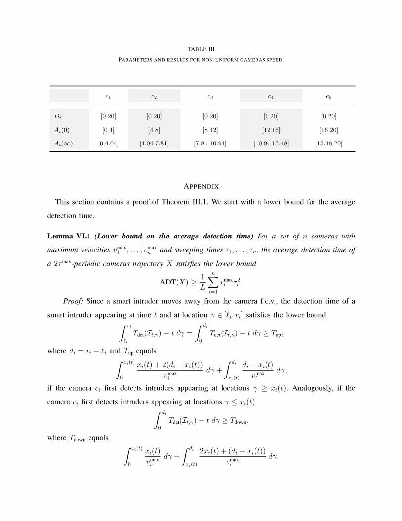
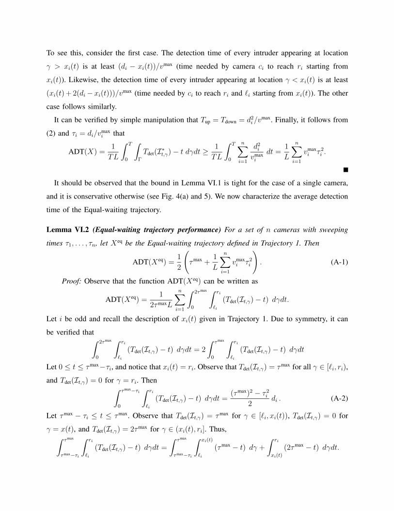
TABLE III
PARAMETERS AND RESULTS FOR NON-UNIFORM CAMERAS SPEED.
c1 c2 c3 c4 c5
Di [0 20] [0 20] [0 20] [0 20] [0 20]
Ai(0) [0 4] [4 8] [8 12] [12 16] [16 20]
Ai(∞) [0 4.04] [4.04 7.81] [7.81 10.94] [10.94 15.48] [15.48 20]
APPENDIX
This section contains a proof of Theorem III.1. We start with a lower bound for the average
detection time.
Lemma VI.1 (Lower bound on the average detection time) For a set of n cameras with
maximum velocities vmax1 , . . . , vmax
n and sweeping times τ1, . . . , τn, the average detection time of
a 2τmax-periodic cameras trajectory X satisfies the lower bound
ADT(X) ≥ 1
L
n∑i=1
vmaxi τ 2
i .
Proof: Since a smart intruder moves away from the camera f.o.v., the detection time of a
smart intruder appearing at time t and at location γ ∈ [`i, ri] satisfies the lower bound∫ ri
`i
Tdet(It,γ)− t dγ =
∫ di
0
Tdet(It,γ)− t dγ ≥ Tup,
where di = ri − `i and Tup equals∫ xi(t)
0
xi(t) + 2(di − xi(t))vmaxi
dγ +
∫ di
xi(t)
di − xi(t)vmaxi
dγ,
if the camera ci first detects intruders appearing at locations γ ≥ xi(t). Analogously, if the
camera ci first detects intruders appearing at locations γ ≤ xi(t)∫ di
0
Tdet(It,γ)− t dγ ≥ Tdown,
where Tdown equals ∫ xi(t)
0
xi(t)
vmaxi
dγ +
∫ di
xi(t)
2xi(t) + (di − xi(t))vmaxi
dγ.
To see this, consider the first case. The detection time of every intruder appearing at location
γ > xi(t) is at least (di − xi(t))/vmax (time needed by camera ci to reach ri starting from
xi(t)). Likewise, the detection time of every intruder appearing at location γ < xi(t) is at least
(xi(t) + 2(di− xi(t)))/vmax (time needed by ci to reach ri and `i starting from xi(t)). The other
case follows similarly.
It can be verified by simple manipulation that Tup = Tdown = d2i /v
max. Finally, it follows from
(2) and τi = di/vmaxi that
ADT(X) =1
TL
∫ T
0
∫Γ
Tdet(I∗t,γ)− t dγdt ≥1
TL
∫ T
0
n∑i=1
d2i
vmaxi
dt =1
L
n∑i=1
vmaxi τ 2
i .
It should be observed that the bound in Lemma VI.1 is tight for the case of a single camera,
and it is conservative otherwise (see Fig. 4(a) and 5). We now characterize the average detection
time of the Equal-waiting trajectory.
Lemma VI.2 (Equal-waiting trajectory performance) For a set of n cameras with sweeping
times τ1, . . . , τn, let Xeq be the Equal-waiting trajectory defined in Trajectory 1. Then
ADT(Xeq) =1
2
(τmax +
1
L
n∑i=1
vmaxi τ 2
i
). (A-1)
Proof: Observe that the function ADT(Xeq) can be written as
ADT(Xeq) =1
2τmaxL
n∑i=1
∫ 2τmax
0
∫ ri
`i
(Tdet(It,γ)− t) dγdt.
Let i be odd and recall the description of xi(t) given in Trajectory 1. Due to symmetry, it can
be verified that∫ 2τmax
0
∫ ri
`i
(Tdet(It,γ)− t) dγdt = 2
∫ τmax
0
∫ ri
`i
(Tdet(It,γ)− t) dγdt
Let 0 ≤ t ≤ τmax−τi, and notice that xi(t) = ri. Observe that Tdet(It,γ) = τmax for all γ ∈ [`i, ri),
and Tdet(It,γ) = 0 for γ = ri. Then∫ τmax−τi
0
∫ ri
`i
(Tdet(It,γ)− t) dγdt =(τmax)2 − τ 2
i
2di . (A-2)
Let τmax − τi ≤ t ≤ τmax. Observe that Tdet(It,γ) = τmax for γ ∈ [`i, xi(t)), Tdet(It,γ) = 0 for
γ = x(t), and Tdet(It,γ) = 2τmax for γ ∈ (xi(t), ri]. Thus,∫ τmax
τmax−τi
∫ ri
`i
(Tdet(It,γ)− t) dγdt =
∫ τmax
τmax−τi
∫ xi(t)
`i
(τmax − t) dγ +
∫ ri
xi(t)
(2τmax − t) dγdt.
Since xi = ri + (t − (τmax − τi)vmaxi ) (see Trajectory 1), it follows from the above expression
that ∫ τmax
τmax−τi
∫ ri
`i
(Tdet(It,γ)− t) dγdt =
∫ τmax
τmax−τi(2τmax − t)di − τmax(τmax − t)vmax
i dt
=1
2τmaxτ 2
i vmaxi +
1
2diτ
2i .
(A-3)
The statement follows by combining (A-2) and (A-3).
We now conclude with a proof of Theorem III.1.
Proof of Theorem III.1: From Lemma VI.1 and VI.2 we have
ADT(Xeq)
ADT∗=
1
2+
Lτmax
2∑n
i=1 vmaxi τ 2
i
=1
2+
Lτmax
2∑n
i=1 diτi≤ 1
2+
Lτmax
τmin2∑n
i=1 di=τmax + τmin
2τmin ,
where we have used L =∑n
i=1 di and τmin ≤ τi for all i ∈ 1, . . . , n. To show the second
bound notice that
ADT(Xeq)
ADT∗=
1
2+
Lτmax
2∑n
i=1 diτi=
1
2+
L
2∑n
i=1 diτiτmax
≤ 1
2+
L
2dmin ,
where the last inequality is obtained by letting τi/τmax → 0 for all i except for one segment
(τi/τmax = 1 for some i, and di ≥ dmin). Since L ≤ ndmax we conclude that
ADT(Xeq)
ADT∗≤ 1
2+ndmax
2dmin ≤(n+ 1)dmax
2dmin .
We now show the last part of the Theorem. Assume that all cameras move at unitary speed
and, without affecting generality, that d1 = dmax. Notice that
ADT(Xeq)
ADT∗=
1
2+
Lτmax
2∑n
i=1 diτi=
1
2+
∑ni=1 d1di
2∑n
i=1 d2i
=1
2
(1 +
1 +∑n
i=2 yi1 +
∑ni=2 y
2i
),
where yi = di/d1. Consider the minimization problem
minK,x2,...,xn
K,
subject to 1 +∑n
i=2 yi ≤ K (1 +∑n
i=2 y2i ) ,
(A-4)
and the associated Lagrangian function [22]
L = K + λ
(1−K +
n∑i=2
yi −Ky2i
).
Following standard optimization theory, necessity optimality conditions for the minimization
problem (A-4) are
∂L∂K
= 0 =⇒ 1− λ(
1 +n∑i=2
y2i
)= 0,
∂L∂yi
= 0 =⇒ λ (1− 2Kyi) = 0, for i ∈ 2, . . . , n,
Complementary slackness: λ
(1−K +
n∑i=2
yi −Ky2i
)= 0.
From the first and second equations we obtain λ 6= 0 and yi = 1/(2K). Then, the third equation
yields K = (1±√n)/2. Since yi > 0, the statement follows.
REFERENCES
[1] J. Clark and R. Fierro, “Mobile robotic sensors for perimeter detection and tracking,” ISA Transactions, vol. 46, no. 1, pp.
3–13, 2007.
[2] D. B. Kingston, R. W. Beard, and R. S. Holt, “Decentralized perimeter surveillance using a team of UAVs,” IEEE
Transactions on Robotics, vol. 24, no. 6, pp. 1394–1404, 2008.
[3] S. Susca, S. Martínez, and F. Bullo, “Monitoring environmental boundaries with a robotic sensor network,” IEEE
Transactions on Control Systems Technology, vol. 16, no. 2, pp. 288–296, 2008.
[4] Y. Elmaliach, A. Shiloni, and G. A. Kaminka, “A realistic model of frequency-based multi-robot polyline patrolling,” in
International Conference on Autonomous Agents, Estoril, Portugal, May 2008, pp. 63–70.
[5] A. Machado, G. Ramalho, J. D. Zucker, and A. Drogoul, “Multi-agent patrolling: An empirical analysis of alternative
architectures,” in Multi-Agent-Based Simulation II, ser. Lecture Notes in Computer Science. Springer, 2003, pp. 155–170.
[6] Y. Chevaleyre, “Theoretical analysis of the multi-agent patrolling problem,” in IEEE/WIC/ACM Int. Conf. on Intelligent
Agent Technology, Beijing, China, Sep. 2004, pp. 302–308.
[7] F. Pasqualetti, A. Franchi, and F. Bullo, “On cooperative patrolling: Optimal trajectories, complexity analysis and
approximation algorithms,” IEEE Transactions on Robotics, vol. 28, no. 3, pp. 592–606, 2012.
[8] M. Baseggio, A. Cenedese, P. Merlo, M. Pozzi, and L. Schenato, “Distributed perimeter patrolling and tracking for camera
networks,” in IEEE Conf. on Decision and Control, Atlanta, GA, USA, Dec. 2010, pp. 2093–2098.
[9] R. Carli, A. Cenedese, and L. Schenato, “Distributed partitioning strategies for perimeter patrolling,” in American Control
Conference, San Francisco, CA, USA, Jun. 2011, pp. 4026–4031.
[10] D. Borra, F. Pasqualetti, and F. Bullo, “Continuous graph partitioning for camera network surveillance,” Automatica, Jul.
2012, submitted.
[11] S. M. Huck, N. Kariotoglou, S. Summers, D. M. Raimondo, and J. Lygeros, “Design of importance-map based randomized
patrolling strategies,” in Complexity in Engineering (COMPENG), Jun. 2012, pp. 1–6.
[12] D. M. Raimondo, N. Kariotoglou, S. Summers, and J. Lygeros, “Probabilistic certification of pan-tilt-zoom camera
surveillance systems,” in IEEE Conf. on Decision and Control and European Control Conference, Orlando, FL, USA,
Dec. 2011, pp. 2064–2069.
[13] M. Spindler, F. Pasqualetti, and F. Bullo, “Distributed multi-camera synchronization for smart-intruder detection,” in
American Control Conference, Montréal, Canada, Jun. 2012, pp. 5120–5125.
[14] F. Zanella, F. Pasqualetti, R. Carli, and F. Bullo, “Simultaneous boundary partitioning and cameras synchronization for
optimal video surveillance,” in IFAC Workshop on Distributed Estimation and Control in Networked Systems, Santa Barbara,
CA, USA, Sep. 2012, pp. 1–6.
[15] R. Bodor, A. Drenner, P. Schrater, and N. Papanikolopoulos, “Optimal camera placement for automated surveillance tasks,”
Journal of Intelligent and Robotic Systems, vol. 50, pp. 257–295, 2007.
[16] J. Zhao, S.-C. Cheung, and T. Nguyen, “Optimal camera network configurations for visual tagging,” IEEE Journal of
Selected Topics in Signal Processing, vol. 2, no. 4, pp. 464 –479, 2008.
[17] C. Soto, B. Song, and A. K. Roy-Chowdhury, “Distributed multi-target tracking in a self-configuring camera network,” in
IEEE Conference on Computer Vision and Pattern Recognition, Miami, FL, USA, Jun. 2009, pp. 1486–1493.
[18] R. Alberton, R. Carli, A. Cenedese, and L. Schenato, “Multi-agent perimeter patrolling subject to mobility constraints,” in
American Control Conference, Montréal, Canada, Jun. 2012, pp. 4498–4503.
[19] J. Czyzowicz, L. Gasieniec, A. Kosowski, and E. Kranakis, “Boundary patrolling by mobile agents with distinct maximal
speeds,” in European Symposium on Algorithms, Saarbrücken, Germany, Sep. 2011, pp. 701–712.
[20] A. Kawamura and Y. Kobayashi, “Fence patrolling by mobile agents with distinct speeds,” in Algorithms and Computation,
ser. Lecture Notes in Computer Science. Springer, 2012, pp. 598–608.
[21] M. Spindler, “Distributed multi-camera synchronization for smart-intruder detection,” Master’s thesis, University of
Stuttgart, Sep. 2011.
[22] S. Boyd and L. Vandenberghe, Convex Optimization. Cambridge University Press, 2004.