Embed Size (px)
Citation preview

MSc: Sustainable Engineering - Energy Systems and the Environment
Cameron L. Smith
Individual Project
(2001 - 2002)
“Energy Efficient Operation of Submersible Borehole Water
Pumps Using Electrical Variable Speed Drives”
Department of Mechanical Engineering
Faculty of Engineering
University of Strathclyde

ii
The copyright of this dissertation belongs to the author under the terms of the United
Kingdom Copyright Acts as qualified by University of Strathclyde Regulation 3.49.
Due acknowledgement must always be made of the use of any material contained in,
or derived from, this dissertation.

iii
Acknowledgements
I wish to express my thanks to Dr. Andrew Grant at the Department of Mechanical
Engineering, University of Strathclyde for supervising this project. I also wish to
thank Kevin Moran at Scottish Water and David Palmer of The Campbell Palmer
Partnership for assisting with the industrial aspect of this project, and Dr. Slobodan
Jovanovic at the Department of Electronic and Electrical Engineering, University of
Strathclyde for his technical assistance.

iv
Contents
List of Tables and Illustrations vi
Abstract viii
Chapter 1 Introduction 1
Chapter 2 Water Pumps 3
2.1 Positive Displacement Pumps 3 2.2 Rotodynamic Pumps 3 2.2.1 Centrifugal Pumps 4 2.2.1.1 Pump Stages 4 2.2.1.2 Pump and System Characteristics 5 2.2.1.3 Flow Control 8 2.2.1.4 The Affinity Laws 11
Chapter 3 Variable Speed Drives 12
3.1 Mechanical Variable Speed Drives 12 3.2 Electrical Variable Speed Drives 12 3.2.1 Induction Motor 12 3.2.2 Frequency Inverters 13 3.2.3 VSD Efficiency 15 3.2.4 VSD Control Loops 15
Chapter 4 Flow Control 17
4.1 Load Duty Cycle 17 4.2 Variable Flow Rate Control 19 4.3 Efficiency Variation with Variable Speed Control 23 4.4 Effect of the Characteristics of the System Curve 24 4.5 Constant Flow Rate Control 25
Chapter 5 Water Pumping Applications 26
5.1 Case 1 - Water Distribution System 26 5.2 Case 2 - Fresh Water Pumping system 28
Chapter 6 Case Study: Spey Wellfields Water Pumping Station 30
6.1 Introduction 30 6.2 Background 30

v
6.3 Pump Models 31 6.4 Nominal Flow Rates 34 6.5 Water Quality Classifications 35 6.6 Pressure Sustaining Valves 36 6.7 System Head Losses 37 6.7.1 Static Head Losses 40 6.7.2 Dynamic Head Losses 40 6.7.2.1 Transmission Main Losses 40 6.7.2.2 Collector Main Losses 42 6.7.2.3 Borehole Piping Losses 42 6.7.3 System Curves 45 6.8 Power Consumption 51 6.8.1 Throttling Control 52 6.8.2 Variable Speed Control 52 6.8.2.1 Pump Efficiency 53 6.9 Demand 57 6.10 Pump Selection 58 6.11 Economics 61 6.12 Further Considerations 63
Chapter 7 Conclusion 65
References 66
Bibliography 67
Appendix A: Pump Efficiency Plots for Variable Speed Control 68
Appendix B: Plots of Power Consumption against Total Flow Rate in Transmission Main 1 - for Individual Pumps 85

vi
List of Tables and Illustrations
Figure 1.1 location of the Spey Wellfields Water Pumping Station 1
Figure 1.2 site location 2
Figure 2.1 pump categories 3
Figure 2.2 types of rotodynamic pump impeller 4
Figure 2.3 impeller arrangements in centrifugal pumps 5
Figure 2.4 example of the characteristic curves of a centrifugal pump 6
Figure 2.5 example of pump curve and system curve 7
Figure 2.6 methods of altering pump flow rate 9-10
Figure 3.1 system components of a frequency inverter 13
Figure 3.2 characteristic waveforms between i/p and o/p
of a frequency inverter 14
Figure 4.1 examples of load duty cycle 18
Figure 4.2 case A: operating points for variable flow control 20
Figure 4.3 case B: operating points for variable flow control 21
Figure 4.4 case C: operating points for variable flow control 22
Figure 4.5 pump efficiency curves at various pump speeds 24
Figure 4.6 characteristic curves for variable speed, constant flow
rate control under conditions of variable system resistance 25
Figure 5.1 schematic of water distribution system 26
Figure 5.2 schematic of fresh water pumping plant 28
Figure 6.1 schematic of Spey Wellfields Water Pumping Station 31
Figure 6.2 Grundfos SP45 and SP27 pump characteristics 34
Figure 6.3 dynamic losses in the transmission mains 41
Figure 6.4 example of dynamic losses in borehole and collector main 45
Figure 6.5 illustration of new axis position for
expressing TDH _ in terms of PQ 46
Figure 6.6 illustration of pump operating range 48
Figure 6.7 example: SYSH vs. TQ 50
Figure 6.8 example: ).( Pm ηη vs. SYSH 54
Figure 6.9 example: ).( Pm ηη vs. TQ 55

vii
Figure 6.10 example: PSVP and VSDP vs. TQ for transmission main 1 56
Figure 6.11 example: PSVP and VSDP vs. TQ for transmission main 2 57
Figure 6.12 VSD feedback control loop 63
Table 6.1 pump performance characteristic data
(reproduced from factory test data) 33
Table 6.2 pump types, water quality, nominal flow rates
and PSV settings 37
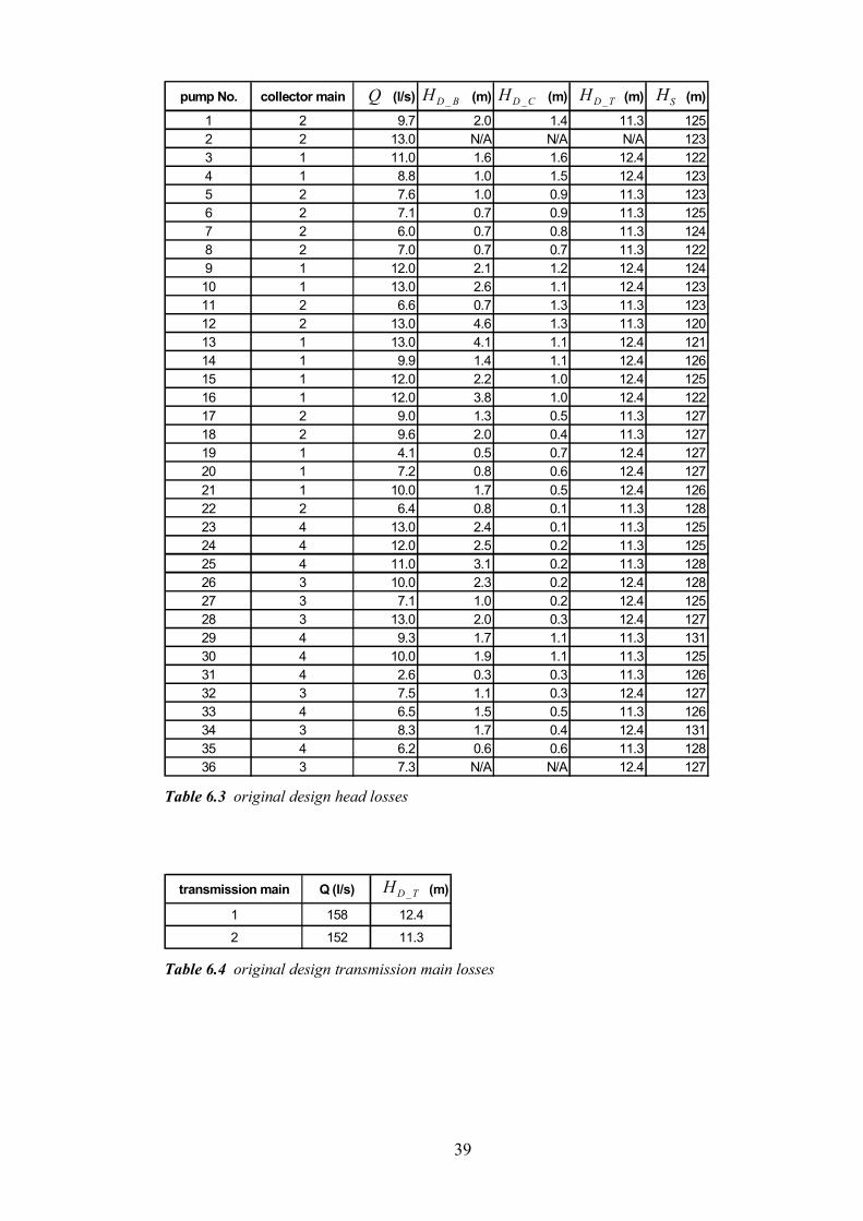
Table 6.3 original design head losses 39
Table 6.4 original design transmission main losses 39
Table 6.5 borehole and collector main head loss coefficients 44
Table 6.6 pump operating ranges: system head and total flow rate 51
Table 6.7 A1 quality pumps: power consumption 59
Table 6.8 selected pumps: power consumption 60
Table 6.9 SP45 pumps: annual energy savings 61
Table 6.10 SP27 pumps: annual energy savings 61
viii
Abstract
Traditionally, water pumping processes have utilised mechanical control devices to
regulate the flow rate delivered by a pump. The most widely used of these devices
are flow control valves. These valves function by inserting additional resistance at
the outlet of a pump. This additional resistance results in lost energy. Over recent
years more interest has been taken in the energy efficiency of water pumping
processes. Flow control is an area which has seen significant development,
particularly in the field of electrical control. Electrical control devices have been
developed, and established in industry, that can perform flow control for many water
pumping applications. These electrical control devices, known as ‘electrical variable
speed drives’, function by regulating the speed of a pump in order to deliver the
required flow rate. For many water pumping applications electrical variable speed
drives provide better energy efficiency than the equivalent mechanical flow control
device. This project is a study into the application of electrical variable speed drives
within water pumping systems. The focus of the study is the energy efficiency
achievable through the use of electrical variable speed drives in comparison to flow
control valves. The study looks at various types of water pumping system, in
relation to specific flow control requirements. A case study is presented of a water
pumping station which uses flow control valves to maintain constant flow rates
delivered by each pump in response to variations in system pressure. An analysis is
made in order to determine the economic viability of installing electrical variable
speed drives in the system to replace the flow control valves. For a given set of flow
conditions, it is shown that energy savings ranging from 9% to 25% can be achieved
on each pump that is operated by an electrical variable speed drive.

1
Chapter 1. Introduction
This project is an investigation into the energy efficiency of pump operation at the
Spey Wellfields Water Pumping Station. The pumping station, which is operated by
Scottish Water, has been in operation since early 1995, and supplies water to the
local public water distribution system. The pumping station is situated on the banks
of the river Spey, in the north east of Scotland. The map below depicts the location.
Figure 1.1 location of the Spey Wellfields Water Pumping Station
The site consists of 36 submersible borehole pumps and two control buildings, the
locations of which are detailed in figure 1.2.

2
Figure 1.2 site plan
The plant currently operates up to 36 pumps, each controlled by a throttling valve to
maintain a constant pump flow rate. When a pump is operating, its motor is running
constantly at full load. Many of the motors are operated in excess of their rated
power capacity. Energy is wasted by throttling the pump discharges. Regular pump
failures are experienced. An investigation was proposed into the excessive power
consumption of the motors, to see if electrical variable speed drives could be used to
economically reduce power consumption, and consequently provide better energy
efficiency and reduce pump failures. This project aims to analyse the pumping
system at the Spey Wellfields Water Pumping Station in order to determine the
potential power reduction and energy savings achievable through the use of electrical
variable speed drives.
1 2 3 4
5 6
7
8
9
10
11 12 13
14 15 16
17 18 19
20 21
2223 24 25 26 27
North ControlBuilding
South Control Building
28 2930
32
31
33 3435 36

3
Chapter 2. Water Pumps
There are several types of water pump. The two main categories are ‘rotodynamic’
and ‘positive displacement’. These are defined by distinctive modes of operation.
Within each of these categories there is a further breakdown into many types of
pump. Figure 2.1 shows the main categories of pump.
Figure 2.1 pump categories
2.1 Positive Displacement Pumps
Positive displacement pumps work on the principle of decreasing the volume of the
boundaries containing the fluid, and so increasing the pressure at the outlet valve,
and allowing the fluid to move into the discharge line. Positive displacement pumps
are best suited to applications for pumping high viscosity fluids, pressure control
applications, and for high pressure, low flow applications.
2.2 Rotodynamic Pumps
Rotodynamic pumps utilise a rotational part, known as an ‘impeller’, to displace
fluid by generating a higher pressure. The direction in which the fluid flows through
PUMPS
ROTODYNAMIC POSITIVE DISPLACEMENT
CENTRIFUGAL MIXED FLOW AXIAL
SINGLE-STAGE MULTI-STAGE

4
the impeller defines the pump type: radial flow (or centrifugal); axial flow; and
mixed flow (for intermediate directions of flow). Figure 2.2 illustrates these types of
impeller, used with rotodynamic pump.
a. radial flow b. mixed flow c. axial flow
Figure 2.2 types of rotodynamic pump impeller
2.2.1 Centrifugal Pumps
For almost all water pumping applications in industry, it is centrifugal pumps that are
used.
2.2.1.1 Pump Stages
Centrifugal pumps are either single-stage or multi-stage. Single-stage pumps have
only one impeller. Multi-stage pumps can have any number of impellers connected
in series. A greater number of impellers (or stages) will generate a higher pressure
for a given flow rate. Figure 2.3 illustrates the arrangement of impellers in single-
stage and multi-stage pumps.

5
a. single-stage b. multi-stage
Figure 2.3 impeller arrangements in centrifugal pumps
2.2.1.2 Pump and System Characteristics
The characteristics of a centrifugal pump are often described by graphs, known as the
‘characteristic curves’. These curves show the head generated by the pump and the
efficiency of the pump, across the range of flow rates at which it can operate. An
example of the characteristic curves of a centrifugal pump is shown in figure 2.4.
The plot showing the head generated by the pump against pump flow rate is known
as the ‘pump curve’.

6
Figure 2.4 example of the characteristic curves of a centrifugal pump
The power absorbed by a pump can be found from the characteristic curves by using
the following equation:
power absorbed, η
ρ.1000... HgQP = (W) (equn. 2.1)
where ρ is liquid density ( 3mkg ), Q is the pump flow rate )( s
l , g is
acceleration due to gravity )( 2sm , H is the head generated by the pump (m)
and η is the wire-to-water efficiency (%)

7
For water at standard conditions, 31000 mkg=ρ . Assuming this value for density is
constant, then the power absorbed by a water pump can be written as:
η
HgQP ..= (W) (equn. 2.2)
A pump would normally be selected such that the head requirement and desired flow
rate occur at the maximum efficiency point. The head requirement is dependent
upon the piping and valve systems through which the output must flow. This can be
broken down into two components of head loss: the dynamic head loss - due to
frictional resistance in the system; and static head loss - the height by which the
water must be raised. The static and dynamic head losses are normally plotted
against the pump curve. This curve, describing total head loss, is referred to as the
‘system curve’, and represents the resistance of the system. Figure 2.5 shows an
example of a system curve, plotted against a pump curve.
Figure 2.5 example of pump curve and system curve
The intersection of the system curve with the H-axis (point A) is the value of static
head loss. The static head loss is independent of the pump flow rate. The curve from
point A to point B represents the dynamic head loss in the system, which is due to

8
frictional losses in the pipework and valves. The dynamic head loss is a function of
the pump flow rate, and can be expressed in the form:
dynamic head loss, 2.QkH D = (m) (equn. 2.3)
where k is a constant and Q is pump flow rate )( sl
So, the system curve can be written in the form:
system head loss, 2.QkHH SSYS += (m) (equn. 2.4)
where SH is static head loss (m)
In the example shown in figure 2.5, it can be seen that the pump overcomes the
system resistance up to point B - where the pump curve and system curve intersect.
Point B, here, is known as the ‘operating point’. Under these conditions the pump
will deliver flow rate, C.
2.2.1.3 Flow Control
If a different flow rate is required, then it may be achieved by one of several
methods. For achieving higher flow rates, possible methods which may be employed
include:
- installing a larger pump
- adding impeller(s) - if the pump physically allows for this, for example, if
impellers have previously been removed
- increasing rotational speed of the pump
- reducing system resistance, for example, installing pipes with less
resistance

9
Lower flow rates may be achieved by the following methods:
- installing a smaller pump
- removing impeller(s)
- trimming impeller(s)
- decreasing rotational speed of the pump
- increasing system resistance, for example, using a throttling valve
Each of these actions can be used to alter the pump flow rate achieved. The effect
that each of these methods has on the pump and system curves is shown, graphically,
in figure 2.6.
a. changing pump or adding/removing stages

10
b. varying pump speed (trimming impellers has a similar effect to reducing pump speed)
c. varying system resistance
Figure 2.6 methods of altering pump flow rate
The method that is used to vary the flow rate or head generated depends upon the
particular requirements of the given pumping system. For example, installing a
larger pump or a smaller pump provides only a crude new operating point, and does
not allow any other setting to be achieved, other than the new operating point.
Trimming impellers to reduce flow rate has more accuracy for setting the operating

11
point, because of the varying degrees to which the impellers can be trimmed, but
again this method does not allow a different operating point to be set when it is
required. Changing the speed of the pump provides far more accuracy for setting the
operating point. Similarly, so too does using a throttling valve. These last two
methods also allow precise control over the operating point. Speed variation and
throttling allow for a range of flow rates to be set, and for the set-point to be
maintained, even under conditions of disturbances in the system resistance or pump
characteristics. As figure 2.6c shows, throttling allows a flow rate to be set by
changing the system curve. Conversely, as figure 2.6b shows, adjusting the pump
speed allows a flow rate to be set by changing the pump curve.
2.2.1.4 The Affinity Laws
When concerned with speed adjustment of a centrifugal load, a group of relationships
known as ‘The Affinity Laws’ provide useful information. These are:
3
2
NPNHNQ
∝
∝∝
where Q is pump flow rate, H is head generated, P is power absorbed and N is pump
speed.
The above relationships are only true when excluding overall system efficiencies,
and assuming zero static system resistance.
The relationship, 2
2
1
2
1
=
NN
HH
, can be used to determine the pump curve for any
pump speed, given the characteristic pump curve at a known speed (as figure 2.6b
illustrates).

12
Chapter 3. Variable Speed Drives
Speed adjustment of a centrifugal pump can be achieved either mechanically or
electrically.
3.1 Mechanical Variable Speed Drives
Mechanical variable speed drives, such as variable ratio belts, variable ratio chains,
variable ratio friction drives and variable ratio gearboxes, can provide speed control
over various centrifugal pump processes. Such mechanical drive systems require the
motor, itself, to operate at full speed and, as such, are subjected to large transmission
losses between motor and pump. Typically, these mechanical drives provide a
transmission efficiency in the range 75% - 80%. Mechanical variable speed drives
require much maintenance, such as lubrication and fine adjustment, in order to
maintain the accuracy of speed settings.
A problem with many pumps, in respect to mechanical variable speed drives, is that
the drives cannot easily be fitted to the system due to the self-contained construction
of many motor-pump units.
3.2 Electrical Variable Speed Drives
Electrical variable speed drives function by converting the electrical signal supplied
to the motor into a form which will vary the speed of rotation of the motor itself.
3.2.1 Induction Motors
The majority of centrifugal pumps are powered by induction motors. It is such
pumps which will be considered hereafter. The rotational speed of an induction
motor is characterised by the following equation:

13
rotational speed, p
fN .120= )( srevs (equn. 3.1)
where f is the frequency of the a.c. supply current (Hz) and p is the No. of
poles
So, for any given number of poles the speed of an induction motor is proportional to
the supply frequency.
3.2.2 Frequency Inverters
The only method of electrically adjusting the speed of an induction motor is to use a
‘frequency inverter’ - a power electronics device which converts the frequency of the
supply signal to a signal of specified frequency. Figure 3.1 shows the main
components of a frequency inverter.
Figure 3.1 system components of a frequency inverter
The rectifier has the function of converting the a.c. input signal to a d.c. signal. The
low-pass filter is used to filter out any a.c. components that are still present in the
waveform. The lower the harmonic content of the waveform at this stage, the less
harmonic distortion there will be at the output of the inverter. The inverter performs
the function of converting the d.c. signal to the required frequency of a.c. signal - to
output to the motor. There are three main different types of inverter section which a
frequency inverter may incorporate. These are: current source inverter (CSI);
variable voltage inverter (VVI); and pulse-width-modulation (PWM) inverter. The
low-pass
filter
i/p
a.c. supply 50Hz
o/p rectifier inverter

14
most common inverter type used with centrifugal pumps is the PWM inverter. The
characteristics of a PWM inverter will, therefore, be described here. The PWM
inverter performs high frequency switching (commonly between 3kHz and 12kHz)
of the d.c. waveform to produce pulses of varying duration (or width), with positive
voltage for half of a cycle and negative voltage for the other half of the cycle. The
width of each pulse is proportional to the voltage of the output waveform. The
switching frequency determines the resolution of the PWM waveform. A higher
switching frequency will provide higher resolution of the PWM waveform, and so,
will give a closer approximation to a pure sine wave at the inverter output, but will
also decrease the efficiency of the drive due to increased heat loss in the drive’s
power components. Figure 3.2 illustrates an example of the waveforms present at
various stages in a frequency inverter.
Figure 3.2 characteristic waveforms between i/p and o/p of a frequency inverter
(The PWM waveform is shown at a greatly reduced switching frequency to illustrate the concept.)

15
Since frequency inverters are the only type of electrical variable speed drive dealt
with hereafter in this text, a frequency inverter is hereafter referred to, exclusively, as
a variable speed drive (VSD).
3.2.3 VSD Efficiency
The typical efficiency of a VSD is approximately 95%, for loads between 30% and
100% of full load [1]. In this region the efficiency is very favourable when
compared to the 75% - 80% efficiency achieved by mechanical variable speed drives.
Below about 30% load the efficiency drops off sharply. For this reason it is not
energy efficient to operate a VSD at the lower end of its speed range.
3.2.4 VSD Control Loops
VSD’s can be used in either open-loop or closed-loop systems. In open-loop
configuration motor speed can be set by specifying the output frequency of the drive.
In closed-loop configuration various system parameters can be set. In water
pumping applications pressure, flow rate and water level could each be used as
reference set-points. A closed-loop system would incorporate sensors, which would
measure the desired parameter, and return, via a transducer, the actual value of that
parameter to the drive. The drive would compare this value to the reference value,
and adjust the output in order to reach the reference set-point. Many VSD’s facilitate
proportional-integral-derivative (PID) control loops. Such control loops allow a high
degree of accuracy in maintaining the reference parameter setting. The controller
output can be described by an equation of the form [2]:
o/pdtdeCdteeK
t
T
... ++= ∫ (equn. 3.2)
where e is the error (ref. - feedback), K is the proportional constant, T is the
integral action time, t is time and C is the derivative constant

16
Each element of the PID controller performs a particular function with respect to the
system’s response time in maintaining the reference set-point. The proportional term
gives an output that is proportional to the error signal. The integral term has the
effect of reducing the offset from the desired reference value. The derivative term is
used to minimize the overshoot, by reducing the oscillations. For a further
explanation of PID controllers the reader is referred to Searle [2].

17
Chapter 4. Flow Control
4.1 Load Duty Cycle
The extent of energy savings achievable through the use of variable speed control in
place of throttling control is dependent upon the specific operational requirements of
the pump under consideration. The load duty cycle of a pump provides essential
information regarding energy savings. This describes the proportion of time for
which the pump is operating, and at what proportion of full load the pump is
operating as a function of percentage of time. Examples of various load duty cycles
are shown in figure 4.1.

18
a. large deviation from full load
b. medium deviation from full load
c. small deviation from full load
Figure 4.1 examples of load duty cycle
10 20 30 40 50 60 70 80 90 100
100
0
% time
% load
10 20 30 40 50 60 70 80 90 100
100
0
% time
% load
10 20 30 40 50 60 70 80 90 100
100
0
% time
% load

19
4.2 Variable Flow Rate Control
Where these load duty cycles refer to varying degrees of flow rate, as determined by
changes in demand, the pump operating points would be determined by the method
of flow control used.
A comparison of these three load duty cycles, for such a case, is given in the example
below. The example compares the two flow control methods of throttling and speed
variation, in terms of power consumption, and resulting energy usage. The period of
operation is taken to be one year.
In tables 4.1, 4.2 and 4.3, Q is pump flow rate, H is head generated, P is power
absorbed and E is energy used. The subscripts “ PSV ” and “VSD ” denote values
referring to throttling control and variable speed control, respectively.

20
CASE A
% flow 30% 40% 50% 60% 70%
% time 10% 20% 40% 20% 10%
Q (l/s) 2.7 3.6 4.4 5.3 6.2
(m) 249 244 238 230 216
(m) 107 112 119 129 138
(kW) 6.6 8.6 10.3 12.0 13.1
(kW) 2.8 4.0 5.1 6.7 8.4
(kWh) 5777 15097 35997 20951 11508
(kWh) 2483 6930 17998 11751 7353
PSVHVSDH
PSVPVSDPPSVEVSDE
Table 4.1
a. throttling control b. variable speed control
Figure 4.2 case A: operating points for variable flow control
Total energy used in one year with throttling control is 89331kWh.
Total energy used in one year with variable speed control is 46514kWh.
Energy saving of 48% with variable speed control.

21
CASE B
% flow 60% 70% 80% 90%
% time 20% 40% 30% 10%
Q (l/s) 5.3 6.2 7.1 8
(m) 230 216 201 190
(m) 129 138 150 164
(kW) 12.0 13.1 14.0 14.9
(kW) 6.7 8.4 10.4 12.9
(kWh) 20951 46034 36792 13062
(kWh) 11751 29411 27456 11275
PSVHVSDH
PSVPVSDPPSVEVSDE
PSVHVSDH
PSVPVSDPPSVEVSDE
Table 4.2
a. throttling control b. variable speed control
Figure 4.3 case B: operating points for variable flow control
Total energy used in one year with throttling control is 116839kWh.
Total energy used in one year with variable speed control is 79893kWh.
Energy saving of 32% with variable speed control.

22
CASE C
% flow 80% 90% 100%
% time 30% 30% 40%
Q (l/s) 7.1 8 8.9
(m) 201 190 179
(m) 150 164 179
(kW) 14.0 14.9 15.6
(kW) 10.4 12.9 15.6
(kWh) 36792 39187 54762
(kWh) 27456 33824 54762
PSVHVSDH
PSVPVSDPPSVEVSDE
PSVHVSDH
PSVPVSDPPSVEVSDE
Table 4.3
a. throttling control b. variable speed control
Figure 4.4 case C: operating points for variable flow control
Total energy used in one year with throttling control is 130740kWh.
Total energy used in one year with variable speed control is 116042kWh.
Energy saving of 11% with variable speed control.

23
From this example it can be seen that greater energy savings can be made when there
is a high concentration of operating time at greatly reduced flow rates.
4.3 Efficiency Variation with Variable Speed Control
There is, however, a limitation to this theory. In the above example, system
efficiencies have not been included.
As stated in chapter 3.2.3, VSD efficiency, VSDη , greatly reduces at very low speeds.
Induction motor efficiency, mη , typically remains fairly constant at around 90% for
loads between 45% and 100% of full load, and significantly reduces at loads below
45% of full load [3]. So, energy savings will not be so significant at low speeds, and
it will, perhaps, be less energy efficient to operate a VSD rather than operating a
throttling valve in this region.
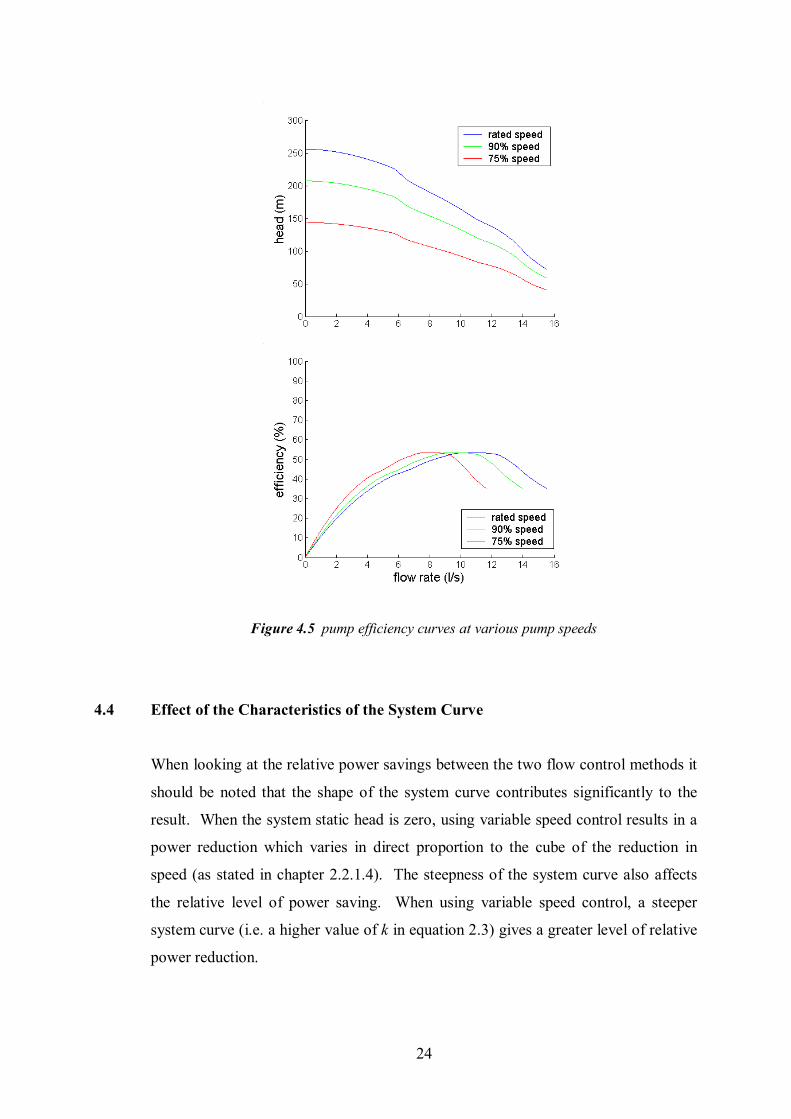
Data on pump efficiency, Pη , is normally provided with pump characteristic curves
in the form of efficiency variation against flow rate for rated pump speed (see figure
2.4). This is sufficient information for determining pump efficiency in the case of
throttling. However, there is a different pump efficiency curve for any given pump
speed. The pump efficiency at a given pump speed and flow rate can be found
through iso-efficiency lines of the form, 2.QkH = . The value of k can be found by
plotting the pump curve for the given pump speed (see chapter 2.2.1.4), and finding
the values of H and Q at the operating point - then 2QHk = . Next, the intersection of
2.QkH = with the pump curve for rated speed can be found, giving a flow rate of
equivalent efficiency for rated speed. Then, since 2.QkH = is an iso-efficiency line,
the required efficiency value can be found by reading the efficiency curve (for rated
pump speed) for this flow rate. Figure 4.5 shows efficiency curves for various pump
speeds, taken by calculating several points and interpolating to give continuous
curves.
24
Figure 4.5 pump efficiency curves at various pump speeds
4.4 Effect of the Characteristics of the System Curve
When looking at the relative power savings between the two flow control methods it
should be noted that the shape of the system curve contributes significantly to the
result. When the system static head is zero, using variable speed control results in a
power reduction which varies in direct proportion to the cube of the reduction in
speed (as stated in chapter 2.2.1.4). The steepness of the system curve also affects
the relative level of power saving. When using variable speed control, a steeper
system curve (i.e. a higher value of k in equation 2.3) gives a greater level of relative
power reduction.

25
4.5 Constant Flow Rate Control
So far this chapter has described systems requiring variable flow rates. Another
scenario in which flow control of a pump may be employed is where a flow rate must
be maintained in response to changes in system pressure requirements. A set flow
rate could be maintained by throttling the pump discharge to a hold certain pressure
under the conditions of a changing system pressure downstream. This form of
control is described by a constant system curve and a constant pump curve. The
alternative to this, using variable speed control, is to change the pump speed in
response to changes in system pressure, so as to hold the desired flow rate. Figure
4.6 shows the characteristic curves of this form of variable speed control.
Figure 4.6 characteristic curves for variable speed, constant flow rate control under
conditions of variable system resistance
For a system with these requirements the load duty cycles shown in figure 4.1 could
describe varying degrees of system pressure (or head) requirements.

26
Chapter 5. Water Pumping Applications
Water pumping is used throughout a range of industries, for various purposes. This
chapter looks at different applications of water pumps where VSD’s have been
implemented, and highlights the energy savings achieved in each system. Two cases
are outlined below.
5.1 Case 1 - Water Distribution System
Figure 5.1 schematic of water distribution system
The requirements of this system are twofold:
1) the borehole water extraction rate must be kept constant, at a
predetermined flow rate, according to the water company’s extraction
contract
distribution points pressure transducer
storage tank
borehole
flowregulating
valve
VSD
VSD
P - Pump
ring main
water flow electrical circuit
pressurerelief valve
frequencysetting
raw water supply
P
P

27
2) a set pressure level in the ring main must be maintained
The original operation of the plant incorporated mechanical control devices. The
borehole pump discharge was throttled by a flow regulating valve in order to
maintain a constant extraction rate. The raw water pump was run at full load, and
pressure in the ring main was maintained by a pressure relief valve, which diverted
excess water back into the storage tank.
The plant was retrofitted with two VSD’s. One was used to control the borehole
pump flow rate - the flow regulating valve was fully opened - and the desired flow
rate maintained by adjusting the speed of the pump. Since no pressure changes occur
downstream, it was sufficient to operate the borehole VSD in open-loop control. The
other VSD was fitted to the raw water pump in a closed loop configuration, with a
pressure transducer providing a feedback signal, representing the measured pressure
at the pump discharge line. The control loop allowed the pressure relief valve to be
fully closed, and ring main pressure to be maintained by automatic adjustment of the
pump speed.
This example highlights two possible uses of VSD’s in water pumping applications:
1) open-loop control to set pump flow rate
2) closed-loop control to hold a pressure set-point in response to downstream
pressure changes
After installation of the VSD’s energy savings of %729 ⋅ for the borehole pump, and
%288 ⋅ for the raw water pump, were recorded. It was calculated that the
installation of the borehole VSD would result in a simple payback of 71⋅ years, and
that the raw water VSD would give a simple payback of 10 months [4].

28
5.2 Case 2 - Fresh Water Pumping System
Figure 5.2 schematic of fresh water pumping plant
In this system water is required to be extracted from the lagoon, stored in two tanks,
and supplied to the respective sand wash plants.
The original system incorporated two manually-operated pumps - one supplying the
red sand storage tank, the other supplying the white sand storage tank. Flow rates
were adjusted, according to demand, by flow regulating valves positioned at each
pump discharge line.
The following alterations were made to the system:
- the flow regulating valves were fully opened
- the red sand tank overflow line was channelled into the white sand tank
red sandwash plant
P P
white sandwash plant
lagoon
red sand tank
white sand tank
waste
waste
flow regulating valves
P - Pump water flow electrical circuit
PP
white sandwash plant
red sandwash plant
lagoon
red sand tank
white sand tank
VSD
valvesfully open
ultrasonic level sensor
overflow
BEFORE AFTER

29
- an ultrasonic level sensor was fitted in the white sand tank, and a VSD
fitted to the white sand pump
With the new configuration no energy was wasted in throttling either pump. Any
excess water in the red sand tank was channelled into the white sand tank. The
ultrasonic level sensor provided a feedback signal to the VSD, which regulated the
speed, and hence flow rate, of the white sand pump - to provide the required volume
of water to the white sand tank.
In this system the VSD is operating in a closed-loop configuration, with liquid level
as the reference parameter.
This case shows an example of the use a VSD for meeting changing flow rate
requirements in response to changes in demand.
The installation of the VSD, along with the replacement of the white sand pump
(with a more appropriately sized one for the new configuration) was calculated to
give a simple payback of 52 ⋅ years [5].

30
Chapter 6. Case Study: Spey Wellfields Water Pumping Station
6.1 Introduction
A scenario which has not yet been fully analysed is the use of a VSD to maintain a
set flow rate in response to changes in downstream pressure. This concept was
introduced in chapter 4.5. The justification for the use of a VSD in such a case is
dependent upon the magnitude of the downstream pressure variations. If the pressure
changes were to cause only small deviations from the desired flow rate, it is unlikely
that the use of a VSD would be financially viable. The initial cost of a throttling
valve is much less than that of a VSD, and the relatively small energy savings made
with a VSD would be far outweighed by the relatively large cost of the VSD. So, in
certain cases, throttling control would be the preferred option in financial terms.
The focus of chapter 6 is a study into the viability of using a VSD to maintain a
constant flow rate in a water pumping system, in which the downstream pressure
varies. The system which is examined, here, is a raw water pumping station,
consisting of 36 borehole pumps, each controlled at a constant flow rate by a
throttling valve. This study looks at the possibility of replacing the throttling valves
with VSD’s as the flow control method, with emphasis on minimising energy
consumption within certain economic criteria.
6.2 Background
The pumping station under investigation, here, is a site operated by Scottish Water.
It is situated on the banks of the River Spey in North East Scotland, grid reference:
NJ 33 57. The site consists of 36 borehole pumps, each extracting water from flood
plain alluvium. The boreholes are mainly supplied by river water, but also partly by
groundwater from west of the wellfield. The boreholes are between 12m and 23m
deep, and are situated at a minimum distance of 50 metres from the river’s edge. The
water is naturally filtered through the alluvial gravels, so only a small amount of
31
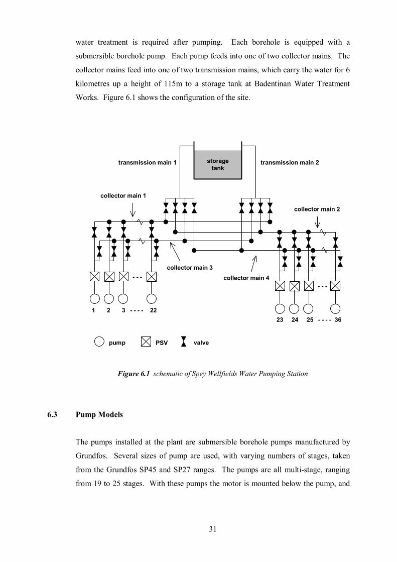
water treatment is required after pumping. Each borehole is equipped with a
submersible borehole pump. Each pump feeds into one of two collector mains. The
collector mains feed into one of two transmission mains, which carry the water for 6
kilometres up a height of 115m to a storage tank at Badentinan Water Treatment
Works. Figure 6.1 shows the configuration of the site.
Figure 6.1 schematic of Spey Wellfields Water Pumping Station
6.3 Pump Models
The pumps installed at the plant are submersible borehole pumps manufactured by
Grundfos. Several sizes of pump are used, with varying numbers of stages, taken
from the Grundfos SP45 and SP27 ranges. The pumps are all multi-stage, ranging
from 19 to 25 stages. With these pumps the motor is mounted below the pump, and
pump valve PSV
storagetank
1 2 3 - - - - 22 23 24 25 - - - - 36
transmission main 2 transmission main 1
collector main 2
collector main 4
collector main 1
collector main 3- - -
- - -

32
is close coupled to the pump. The electricity supply is a dedicated 3-phase supply
line, with each phase at 415V, 50Hz. The SP27 pumps are fitted with 6” Grundfos 3-
phase induction motors rated at kW518 ⋅ , with a full load current of A539 ⋅ . The
SP45 pumps are fitted with 8” Franklin 3-phase induction motors rated at 30kW, with
a full load current of A062 ⋅ . All motors are connected in delta configuration. Due
to the close coupling of the motor and pump, any form of mechanical speed control
is practically unsuitable with these pumps.
Factory test data, providing performance characteristics, relating flow rate, head
generated and wire-to-water efficiency, for each pump is reproduced in table 6.1.
The values given for efficiency include motor efficiency, mη , and pump efficiency,
Pη .

33
Table 6.1 pump performance characteristic data (reproduced from factory test data)
Figure 6.2 shows plots of the data given in table 6.1, with interpolation of the data
points. These curves can be used to determine pump operating ranges, and to
determine the relationship between head generated, flow rate and efficiency for any
point within the operating range.
Q (l/s) H (m) (%)
SP27-210.00 247.4 0.001.11 240.6 13.152.22 N/A 24.303.89 207.6 37.915.56 185.0 48.436.67 160.9 51.867.78 134.3 51.888.89 110.6 48.469.44 93.5 42.26
10.00 78.0 37.80SP27-23
0.00 247.5 0.001.11 244.3 12.142.22 233.8 22.913.89 220.2 26.945.56 201.2 47.786.67 180.7 54.197.78 153.0 56.788.89 124.4 56.769.44 110.0 52.26
10.00 91.7 48.03SP45-19
0.00 232.2 0.005.56 204.9 40.466.67 188.9 44.287.78 174.9 44.908.89 162.1 50.72
10.00 149.9 53.0111.11 133.7 52.8812.22 120.9 51.6613.33 107.3 48.4514.44 88.1 42.1715.56 68.3 36.65
η Q (l/s) H (m) (%)
SP45-210.00 255.8 0.005.56 228.0 41.306.67 207.3 44.617.78 193.0 48.498.89 179.3 51.40
10.00 164.4 53.3011.11 147.8 53.4212.22 135.0 52.6613.33 116.9 48.0514.44 90.7 40.8015.56 72.2 35.20
SP45-240.00 282.6 0.005.56 256.3 41.526.67 234.2 45.087.78 219.2 49.258.89 205.1 52.68
10.00 192.6 56.0811.11 173.3 56.2412.22 151.2 53.2313.33 133.3 49.4814.44 105.8 41.4915.56 76.8 35.42
SP45-250.00 299.0 0.005.56 265.7 41.146.67 242.5 45.427.78 226.6 49.648.89 211.8 53.01
10.00 194.0 54.9911.11 173.4 54.9412.22 157.6 52.2913.33 133.9 48.4614.44 111.3 42.6215.56 52.4 41.25
η

34
Figure 6.2 Grundfos SP45 and SP27 pump characteristics
6.4 Nominal Flow Rates
During the initial design stages, tests were carried out on each borehole to determine
the maximum extraction rate which could be sustained whilst maintaining sufficient

35
water levels in each borehole well. The pumps were selected, and the system
designed, such that any pump operating could extract water at the required
sustainable rate for that well. The maximum flow rate that each pump can sustain
will be referred to as its ‘nominal flow rate’, alnoQ min (see table 6.2 for a list of
nominal flow rates).
The nominal flow rate is required to be maintained in response to any changes in
system resistance. The most significant fluctuation in system resistance occurs as a
result of the number of pumps operating through any given collector main or
transmission main. The more pumps that are operating through a main, the greater
the resistance seen by any pump connected to that main.
The piping system, which each pump feeds into, consists of two collector mains for
pumps on the south bank, and two collector mains for pumps on the north bank (as
shown in figure 6.1). Pumps 1 - 22 (on the south bank) can be connected to either
collector main 1 or collector main 2. Similarly, pumps 23 - 36 (on the north bank)
can be connected to either collector main 3 or collector main 4. At the
interconnection between the collector mains and transmission mains, a set of valves
allow the connection of any collector main to either transmission main. So, any
configuration of collector main and transmission main is possible - the only
limitation being that pumps on the south bank can only be connected to collector
mains 1 and 2, and pumps on the north bank can only be connected to collector
mains 3 and 4. The transmission mains feed into the top of the storage tank - above
the water level - so the pumps are not working against any pressure changes due to
water level in the storage tank.
6.5 Water Quality Classifications
Each well provides water with different concentrations of iron and manganese, which
constitute different levels of water quality. Classifications exist for various degrees
of water quality. The classifications are A1, A2, B1 and B2, in order of quality -
highest to lowest. Table 6.2 lists the water quality classifications for each well.
36
6.6 Pressure Sustaining Valves
The system was originally designed to have pressure sustaining valves (PSV’s) fitted
to the discharge line of each pump. The PSV’s perform the function of throttling the
pump discharge in order to maintain a constant head seen by each pump, which
corresponds to the nominal flow rate on the respective pump curve. The amount of
throttling is automatically adjusted in response to changes in downstream pressure -
when pumps are switched on or switched off - to maintain a constant pressure at the
pump discharge line and, hence, maintain constant flow rate.
Pumps were selected for each borehole on the basis of the ability of the pumps to
meet nominal flow rates under conditions of maximum expected system resistance,
so that the nominal flow rates could be achieved under any normal operating
conditions. Table 6.2 lists the pump type selected for each borehole, and the pressure
setting for each PSV that gives the nominal flow rate for each pump (based on the
pump characteristic curves shown in figure 6.2).

37
pump No. pump type water quality (l/s) PSV setting (m)
1 SP45-25 A1 11.75 164.52 SP45-25 A2 12.00 N/A3 SP45-24 A1 12.00 155.44 SP45-19 A1 9.20 158.75 SP45-19 A1 10.00 149.96 SP27-21 A1 7.20 148.17 SP27-21 A2 7.16 149.18 SP27-23 A1 7.00 173.09 SP45-24 A1 11.30 169.710 SP45-25 A1 12.00 161.111 SP45-19 A1 9.30 157.712 SP45-25 A1 12.20 158.013 SP45-25 A1 12.10 159.614 SP45-21 A1 10.70 153.715 SP45-25 A1 12.20 158.016 SP45-25 A1 12.10 159.617 SP45-21 A2 10.69 153.918 SP45-25 A1 12.50 152.319 SP27-23 A1 7.13 169.820 SP27-23 A1 7.50 160.221 SP45-25 A1 12.20 158.022 SP45-19 A1 9.20 158.723 SP45-25 A1 12.50 152.324 SP45-25 A1 12.20 158.025 SP45-25 A1 12.10 159.626 SP45-25 B2 12.20 158.027 SP45-24 A1 11.70 161.528 SP45-25 A2 12.00 161.129 SP45-25 B2 11.90 162.530 SP45-21 B1 10.70 153.731 SP27-21 A2 7.14 149.632 SP27-23 A1 7.13 169.833 SP45-21 A1 10.71 153.634 SP45-21 A1 10.54 156.235 SP27-23 A1 7.13 169.836 SP27-23 N/A 7.00 N/A
alnoQ min
Table 6.2 pump types, water quality, nominal flow rates and PSV settings
6.7 System Head Losses
In order to calculate the amount of the throttling employed on each pump discharge
line, and the potential energy reductions resulting from variable speed operation of
the pumps, the range of system resistance seen by each pump with the PSV’s fully
open must be analysed. This involves modelling the head losses incurred in the

38
borehole piping, the collector mains and the transmission mains. As stated in chapter
6.4 the resistance seen by any one pump varies depending on the number of pumps
operating through the same collector main or transmission main as that pump. The
analysis in chapter 6.7 looks at the resistance seen by each pump when the PSV’s are
fully open. In the original design of the system, calculations were made describing
head losses in each borehole, collector main and transmission main under certain
flow conditions. The analysis describes the situation when all pumps are operating
(except pumps No.2 and No.36) with flow rates and mains configuration as given in
tables 6.3 and 6.4. All calculations in this chapter are made on the assumption that
pump and collector main connections are as shown in table 6.3.
39
pump No. collector main (l/s) (m) (m) (m) (m)
1 2 9.7 2.0 1.4 11.3 1252 2 13.0 N/A N/A N/A 1233 1 11.0 1.6 1.6 12.4 1224 1 8.8 1.0 1.5 12.4 1235 2 7.6 1.0 0.9 11.3 1236 2 7.1 0.7 0.9 11.3 1257 2 6.0 0.7 0.8 11.3 1248 2 7.0 0.7 0.7 11.3 1229 1 12.0 2.1 1.2 12.4 12410 1 13.0 2.6 1.1 12.4 12311 2 6.6 0.7 1.3 11.3 12312 2 13.0 4.6 1.3 11.3 12013 1 13.0 4.1 1.1 12.4 12114 1 9.9 1.4 1.1 12.4 12615 1 12.0 2.2 1.0 12.4 12516 1 12.0 3.8 1.0 12.4 12217 2 9.0 1.3 0.5 11.3 12718 2 9.6 2.0 0.4 11.3 12719 1 4.1 0.5 0.7 12.4 12720 1 7.2 0.8 0.6 12.4 12721 1 10.0 1.7 0.5 12.4 12622 2 6.4 0.8 0.1 11.3 12823 4 13.0 2.4 0.1 11.3 12524 4 12.0 2.5 0.2 11.3 12525 4 11.0 3.1 0.2 11.3 12826 3 10.0 2.3 0.2 12.4 12827 3 7.1 1.0 0.2 12.4 12528 3 13.0 2.0 0.3 12.4 12729 4 9.3 1.7 1.1 11.3 13130 4 10.0 1.9 1.1 11.3 12531 4 2.6 0.3 0.3 11.3 12632 3 7.5 1.1 0.3 12.4 12733 4 6.5 1.5 0.5 11.3 12634 3 8.3 1.7 0.4 12.4 13135 4 6.2 0.6 0.6 11.3 12836 3 7.3 N/A N/A 12.4 127
BDH _ CDH _ SHTDH _Q
Table 6.3 original design head losses
transmission main Q (l/s) (m)
1 158 12.4
2 152 11.3
TDH _
Table 6.4 original design transmission main losses

40
6.7.1 Static Head Losses
The static head losses for each pump are listed in table 6.3.
6.7.2 Dynamic Head Losses
When only one pump is operating through a particular collector main and
transmission main, then the system resistance can be described by an equation of the
form:
system resistance, 2. PSSYS QKHH += (equn. 6.1)
where SH is static head, K is a constant and PQ is the pump flow rate
The term 2. PQK describes the combined dynamic losses incurred in the borehole
piping, collector main and transmission main.
However, when more pumps are brought into line, the losses in the collector main
and transmission main become dependent on, not only PQ , but on the total flow rate
in the collector main and in the transmission main (including PQ ).
6.7.2.1 Transmission Main Losses
Dynamic losses through the transmission mains can be described by an equation of
the form:
dynamic losses in transmission main n, 2)()()(_ . nTnTnTD QkH = (equn. 6.2)
where )(nTk is a constant and )(nTQ is the total flow rate through the
transmission main

41
Using the values given in table 6.4, )1(Tk and )2(Tk can be found, as described below:
when slQT 158)1( = , mH TD 4.12)1(_ =
when slQT 152)2( = , mH TD 3.11)2(_ =
substituting into equation 6.2 gives:
00049670158
4122)1(
⋅=
⋅=Tk
00048900152
3112)2(
⋅=
⋅=Tk
Figure 6.3 shows plots of the dynamic losses in the transmission mains.
Figure 6.3 dynamic losses in the transmission mains

42
6.7.2.2 Collector Main Losses
Head losses in the collector mains, also, vary depending upon the number of pumps
operating through a given collector main. Unlike the intersection of the collector
mains with the transmission mains, the connections of the pump discharge lines to
the collector mains do not occur at a common point. Each pump connects to a
different section of the collector mains. Due to this configuration, the calculation of
collector main losses as a function of total flow rate through a collector main can
only be made for a given sequence of pump switching, since the output of the pumps
only flow through certain sections of a collector main, and so the resistance seen by
one pump depends upon the point of connection of the other pumps to the collector
main, as well as the flow rates of the pumps. For the purposes of carrying out power
calculations, here, collector mains head losses are assumed to be independent of the
total flow rate through the collector mains, and will be assumed to vary only with
pump flow rate. Thus, dynamic losses in the collector mains can be expressed in the
form:
dynamic losses in a collector main, 2_ . PCCD QkH = (equn. 6.3)
where Ck is a constant
Using the values of CDH _ given in table 6.3, values for Ck , found from equation 6.3,
are given for each pump in table 6.5. The conditions governing these values of Ck
are for 34 pumps operating, which is close to the maximum capacity. So, the values
of Ck given in table 6.5 can be considered as approximately “worst case” values.
6.7.2.3 Borehole Piping Losses
Dynamic losses in the borehole piping of each pump are independent of total flow
rate, since the flow from one pump does not travel through the borehole piping of
any other pump. So, the losses are dependent only on the flow rate of the pump

43
concerned. Dynamic losses in the borehole piping can be described by an equation
of the form:
2_ . PBBD QkH = (equn. 6.4)
where Bk is a constant
Using the values of BDH _ given for each pump in table 6.3, values for Bk , found
from equation 6.4, are given for each pump in table 6.5.

44
pump No.
1 0.02126 0.014882 N/A N/A3 0.01322 0.013224 0.01291 0.019375 0.01731 0.015586 0.01389 0.017857 0.01944 0.022228 0.01429 0.014299 0.01458 0.0083310 0.01538 0.0065111 0.01607 0.0298412 0.02722 0.0076913 0.02426 0.0065114 0.01428 0.0112215 0.01528 0.0069416 0.02639 0.0069417 0.01605 0.0061718 0.02170 0.0043419 0.02974 0.0416420 0.01543 0.0115721 0.01700 0.0050022 0.01953 0.0024423 0.01420 0.0005924 0.01736 0.0013925 0.02562 0.0016526 0.02300 0.0020027 0.01984 0.0039728 0.01183 0.0017829 0.01966 0.0127230 0.01900 0.0110031 0.04438 0.0443832 0.01956 0.0053333 0.03550 0.0118334 0.02468 0.0058135 0.01561 0.0156136 N/A N/A
Bk Ck
Table 6.5 borehole and collector main head loss coefficients
The combined borehole piping and collector main losses for pump No.1 is plotted in
figure 6.4.

45
Figure 6.4 example of dynamic losses in borehole and collector main
6.7.3 System Curves
Since the total flow rate in a transmission main, TQ , is the only variable determining
the total head loss seen by each pump, then it is useful to find the system curves for
various values of TQ . In order to plot the system curve of any pump for a given
value of TQ , the equations describing the borehole, collector main and transmission
main head losses must be expressed in terms of PQ , for the given value of TQ .
Collector main and borehole piping losses are independent of TQ , and are expressed
in a form in terms of PQ in equations 6.3 and 6.4, respectively. The transmission
main losses are expressed in terms of TQ in equation 6.2. To express equation 6.2 in
terms of PQ , for a particular pump, the TQ -axis must be shifted to the left by an
amount, X, such that (see figure 6.5):

46
alnoT QQX min'−= (equn. 6.5)
where 'TQ is the value of TQ for which expression must be found and
alnoQ min is the nominal flow rate of the pump
Figure 6.5 illustration of new axis position for expressing TDH _ in terms of PQ
The PQ - axis is related to the TQ - axis by the expression:
PT QXQ =−
XQQ PT += (equn. 6.6)
substituting into equation 6.2 gives,
2
_ ).( XQkH pTTD +=
)..2.( 22 XQXQk PPT ++= (equn. 6.7)

47
So, the complete system curve can be described, for any given value of TQ , by the
following equation:
TDCDBDSSYS HHHHH ___ +++=
2222 ....2... XkQXkQkQkQkH TPTPTPCPBS +++++=
22 ....2).( XkHQXkQkkk TSPTPTCB +++++= (equn. 6.8)
Figure 6.6 shows a plot of the pump curve, for pump No.1, and the system curve
occurring at three significant states (when pump No.1 is connected through
transmission main 1).
With only pump No.1 operating, system curve S1 would occur (with the PSV fully
open). In this condition, using throttling control, the PSV would produce the largest
resistance that it is required to do, in order to produce system curve S4 and force the
operating point to point B (which is the only operating point that will give the
nominal flow rate at rated pump speed). Using variable speed control, the pump
speed would reduce and provide pump curve P2 and the pump would operate at point
A.

48
Figure 6.6 illustration of pump operating range
As more pumps are brought into line, system resistance increases. Line S3
represents the system curve when all pumps are operating through transmission main
1. With this level of resistance the system curve has gone beyond point B, and the
pump can only be operated at flow rates less than nominal flow rate. The maximum
system resistance for which nominal flow rate can be maintained is when system
curve S2 occurs. With this system resistance the pump will operate at point B
(nominal flow rate) with the PSV fully open and the pump running at full speed
under either throttling or variable speed control. The range of system head loss for
which nominal flow rate can be maintained (given that curve S1 represents the
minimum system resistance) is between point A and point B. For pump No.1 the
system head range at nominal flow rate is m0130 ⋅ to m5164 ⋅ . Since the change in
system resistance at nominal flow rate is dependent only upon total flow rate in the
transmission main, TQ , then the system head between point A and point B can be
expressed as a function of TQ . This relationship can be found by looking at equation
6.7. For nominal flow rate equation 6.7 is valid for 51640130 ⋅<<⋅ SYSH (the range

49
of system head between point A and point B when connected to transmission main
1). The maximum value of TQ in this range can be found from equation 6.2:
s
lQ
Q
T
T
5263
.000496705164 2
⋅=⇒
⋅=⋅
The system resistance at point A is independent of TQ , so when expressing system
resistance at nominal flow rate as a function of TQ , then the value of system head at
point A is a constant. At nominal flow rate the minimum flow through the
transmission main is the flow rate of the pump itself, i.e. the nominal flow rate.
Hence, when expressing system resistance at nominal flow rate as a function of TQ ,
the minimum value of TQ for which the expression is valid is the value of the
nominal flow rate of the pump itself. For pump No.1 connected through
transmission main 1, the system resistance at nominal flow rate, expressed as a
function of TQ is given by:
2.000496700130 TSYS QH ⋅+⋅= , for 5.2637511 <<⋅ TQ (equn. 6.9)
Equation 6.9 is plotted in figure 6.7.

50
Figure 6.7 example: SYSH vs. TQ
The general form of equation 6.9 is:
2min . TTSYS QkHH += , for max_min TTalno QQQ << (equn. 6.10)
where minH is the minimum system head loss seen by a pump at nominal
flow rate (defined for the condition where no other pumps are operating - for
pump No. 1 this is point A on figure 6.6) and T
T kH
Q maxmax_ = , where
maxH is the maximum allowable system head loss at nominal flow rate (i.e.
the head value corresponding to nominal flow rate on the pump curve for full
speed - for pump No. 1 this is point B on figure 6.6)
The constants in equation 6.10 are given for each pump in table 6.6.

51
pump No. (m) (m) (l/s) (l/s) (l/s)
1 130.0 164.5 11.75 263.5 265.62 N/A N/A 12.00 N/A N/A3 125.9 155.4 12.00 243.7 245.64 125.7 158.7 9.20 257.8 259.85 126.9 149.9 10.00 215.2 216.96 126.6 148.1 7.20 208.1 209.77 126.1 149.1 7.16 215.2 216.98 123.4 173.0 7.00 316.0 318.49 127.6 169.7 11.30 291.1 293.410 126.2 161.1 12.00 265.1 267.211 127.0 157.7 9.30 248.6 250.612 125.3 158.0 12.20 256.6 258.613 125.6 159.6 12.10 261.6 263.714 128.9 153.7 10.70 223.4 225.215 128.4 158.0 12.20 244.1 246.016 127.0 159.6 12.10 256.2 258.217 129.5 153.9 10.69 221.6 223.418 131.1 152.3 12.50 206.6 208.219 130.6 169.8 7.13 280.9 283.120 128.5 160.2 7.50 252.6 254.621 129.3 158.0 12.20 240.4 242.322 129.9 158.7 9.20 240.8 242.723 127.4 152.3 12.50 223.9 225.724 127.9 158.0 12.20 246.2 248.125 132.1 159.6 12.10 235.3 237.126 131.9 158.0 12.20 229.2 231.027 128.3 161.5 11.70 258.5 260.628 129.0 161.1 12.00 254.2 256.229 135.7 162.5 11.90 232.3 234.130 128.4 153.7 10.70 225.7 227.531 130.5 149.6 7.14 196.1 197.632 128.3 169.8 7.13 289.1 291.333 131.4 153.6 10.71 211.4 213.134 134.4 156.2 10.54 209.5 211.135 129.6 169.8 7.13 284.5 286.736 N/A N/A 7.00 N/A N/A
alnoQ minminH maxH max_)1(TQ max_)2(TQ
Table 6.6 pump operating ranges: system head and total flow rate
6.8 Power Consumption
The difference in power consumption between throttling control and variable speed
control for each pump is examined in chapter 6.8.

52
6.8.1 Throttling Control
When a PSV is being used to maintain nominal flow rate, the pump operating point
remains the same (point B of figure 6.6). Since the operating point does not change,
then H, Q and η are constant. So, when using a PSV, the power consumption can be
expressed as (as stated in equation 2.2):
Pm
SYSPPSV
HgQP
ηη ...
= (equn. 6.11)
PSVP is a constant at nominal flow rate.
6.8.2 Variable Speed Control
When using a VSD to maintain nominal flow rate the operating point will vary
(between point A and point B of figure 6.6) depending upon total flow rate, TQ . So
SYSH will vary with TQ , and Pη will vary as pump speed changes - also as a
function of TQ . Motor efficiency, mη , is assumed to remain constant over the
operating range considered here. There is a further factor which must be brought
into the power calculation - the efficiency of the VSD, VSDη . This will be taken to be
constant, such that 950 ⋅=VSDη . Power consumption, when using a VSD to
maintain nominal flow rate, can be expressed as a function of TQ using the equation:
)(..)(..
TPVSDm
TSYSPVSD Q
QHgQP
ηηη= (equn. 6.12)
where )( TSYS QH represents SYSH expressed as a function of TQ , and
)( TP Qη represents Pη expressed as a function of TQ

53
The relationship between SYSH and TQ for each pump can be found from equation
6.10 and table 6.6. The relationship between Pη and TQ for variable speed control
is examined in chapter 6.8.2.1.
6.8.2.1 Pump Efficiency
Since the efficiency curve and pump curve are not described by equations, but only
as plots, graphical methods must be used to find the relationship between Pη and TQ
for variable speed control. Firstly, using the method described in chapter 4.3, a plot
of Pη against SYSH can be found.
It should be noted that the efficiency values given in table 6.1 include motor
efficiency, mη , and pump efficiency, Pη . Within the operating range considered
here, mη would be expected to remain constant. Similarly, mη would be expected to
remain constant across the range for which Pη varies with speed variation. So, given
that mη is taken to be a constant, there is no need to separate mη and Pη when
calculating the variation of Pη with TQ . It is sufficient to plot motor and pump
efficiency ( Pm ηη . ) against TQ under these assumptions.
A computer program was used to find various values of k for a sequence of curves of
the form, 2.QkH = , each passing through a different point between minH and maxH
at nominal flow rate. With the program, the intersection of each of these curves with
the pump curve (for rated speed) was found. Then, for each point found on the pump
curve, the efficiency at that flow rate was read from the efficiency curve (for rated
speed). Then, these efficiency values were plotted against the initial values of SYSH
to show the variation of motor and pump efficiency with system head at nominal
flow rate, between minH and maxH . This plot, for pump No.1, is shown in figure 6.8.

54
Figure 6.8 example: ).( Pm ηη vs. SYSH
The H-axis can be translated from SYSH to TQ by finding TQ for various points on
the curve using equation 6.9. Motor and pump efficiency ( Pm ηη . ) can then be
plotted against TQ . Figure 6.9 shows a plot of ( Pm ηη . ) against TQ for pump No.1
connected through transmission main 1. Plots of ( Pm ηη . ) against TQ for each pump
are contained in appendix A.
55
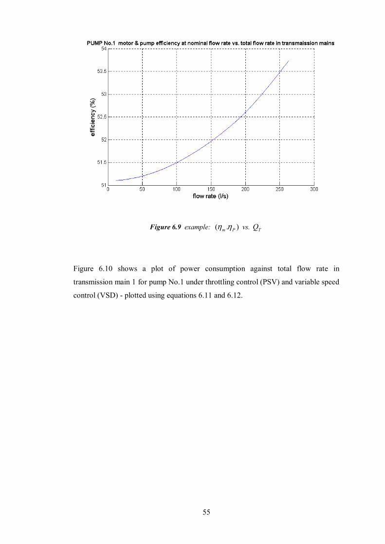
Figure 6.9 example: ).( Pm ηη vs. TQ
Figure 6.10 shows a plot of power consumption against total flow rate in
transmission main 1 for pump No.1 under throttling control (PSV) and variable speed
control (VSD) - plotted using equations 6.11 and 6.12.

56
Figure 6.10 example: PSVP and VSDP vs. TQ for transmission main 1
It can be seen that, at max_TQ , power consumption with the VSD is greater than the
power consumption with the PSV. In this condition, with throttling control the PSV
would be fully open (i.e. the PSV is would not be creating any additional system
resistance), and with variable speed control the pump would be operating at full
speed. The additional power consumed with variable speed control is as a result of
the additional efficiency factor of the VSD, VSDη .
Figure 6.11 shows the power consumption for pump No.1, when connected to
transmission main 2. By comparing figures 6.10 and 6.11 it can be seen that, for
variable speed control, the difference in power consumption between transmission
main 1 and transmission main 2 is insignificant to this degree of accuracy.

57
Figure 6.11 example: PSVP and VSDP vs. TQ for transmission main 2
Plots of PSVP and VSDP against TQ for each pump are given in appendix B. Only the
plots for connection to transmission main 1 are given. The plots for connection to
transmission main 2 can be assumed to be the same.
Due to differences in the pump and system characteristics, and differences in
nominal flow rates for each pump, the difference in power consumption between
throttling control and variable speed control, for a given system state, varies from
pump to pump. So, certain pumps are likely yield greater benefits when installed
with VSD’s than others, depending on the load duty cycle of each pump.
6.9 Demand
An estimated demand profile, provided by Scottish Water, was used, here, to
examine the energy savings which could be achieved by installing VSD’s. The
forecast demand data is in the form of annual average flow rates. An analysis was

58
carried out using the forecast demand for the year 2003. The average water demand,
forecast for 2003, is estimated at approximately sl197 . This flow rate was used for
the analysis of pump operation over the year.
6.10 Pump Selection
The factors which must be taken into account when looking at the viability of
installing VSD’s on pumps are power consumption and water quality. For the
analysis of the year 2003 the total flow rate, at sl197 , is approximately 53% of the
maximum capacity of all the pumps. This suggests that around 19 pumps (depending
on the individual flow rates) would be required to meet the demand flow rate. So, 19
pumps must be selected from the total of 36 pumps. The first selection factor to be
considered is water quality. There are 27 A1 quality pumps (see table 6.2), so the
first selection was made by short-listing these 27 high water quality pumps. Since
the purpose of this study is to analyse the potential energy savings achievable
through the use of VSD’s in the present system, then the final pump selection was
based on the magnitude of energy savings for each pump. The energy savings are a
measure of the difference between PSVP and VSDP for a particular pump, in relation to
the length of time for which that pump is operating over a period. Since all the
pumps in this analysis are operating constantly over the year, the energy savings
made on a pump are directly proportional to the power reduction in that pump.
Using the plots given in appendix B, the pumps can be listed in order of annual
energy savings made with VSD’s, at a given flow configuration. Initially, the power
reduction was calculated on the basis of an equal flow rate through each transmission
main, i.e. sl598 ⋅ in each transmission main, making up the total flow rate of
sl197 . It is desirable to have equal flow rates in each transmission main in order to
minimize head losses, since 2_ QH TD ∝ . Table 6.7 shows the power reduction for
each A1 quality pump for these flow conditions, listed in order of magnitude of
power reduction.

59
pump No. (kW) (kW) power reduction (kW)
8 21.5 16.3 5.29 33.5 28.9 4.64 27.7 23.4 4.332 21.3 17.3 4.035 21.3 17.4 3.910 35.8 32.0 3.811 27.7 23.9 3.813 36.0 32.2 3.81 35.3 31.8 3.512 36.1 32.6 3.516 36.0 32.5 3.522 27.7 24.2 3.527 33.7 30.4 3.319 20.8 17.6 3.224 36.1 33.1 3.015 36.1 33.2 2.93 33.9 31.1 2.821 36.1 33.4 2.720 20.9 18.2 2.714 30.2 27.7 2.525 36.0 33.5 2.55 27.7 25.5 2.223 36.3 34.2 2.133 30.2 28.2 2.034 30.3 28.4 1.96 20.2 18.8 1.418 36.3 34.9 1.4
PSVP VSDP
Table 6.7 A1 quality pumps: power consumption
Starting from the top of table 6.7, pumps were chosen to give a total flow rate of
approximately sl197 . The first 19 pumps in the table (down to and including pump
No.20) give a total flow rate of sl34195 ⋅ , which is sufficiently close to the
estimated demand figure for this analysis. With this set of pumps operating, the
power reduction for each pump must be re-calculated for the new values of flow rate
in each transmission main. With the same configuration of pumps and collector
mains, as described in chapter 6.7, the flow rates through each collector main are as
follows:
60
collector main 1: sl5395 ⋅
collector main 2: sl4552 ⋅
collector main 3: sl8318 ⋅
collector main 4: sl5328 ⋅
Connecting collector mains 1 and 3 to transmission main 1, and collector mains 2
and 4 to transmission main 2 gives the most even split of the total flow. This results
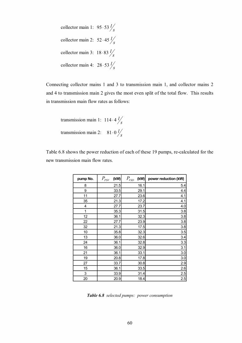
in transmission main flow rates as follows:
transmission main 1: sl4114 ⋅
transmission main 2: sl081⋅
Table 6.8 shows the power reduction of each of these 19 pumps, re-calculated for the
new transmission main flow rates.
pump No. (kW) (kW) power reduction (kW)
8 21.5 16.1 5.49 33.5 29.1 4.411 27.7 23.6 4.135 21.3 17.2 4.14 27.7 23.7 4.01 35.3 31.5 3.812 36.1 32.3 3.822 27.7 23.9 3.832 21.3 17.5 3.810 35.8 32.3 3.513 36.0 32.6 3.424 36.1 32.8 3.316 36.0 32.9 3.121 36.1 33.1 3.019 20.8 17.8 3.027 33.7 30.8 2.915 36.1 33.5 2.63 33.9 31.4 2.520 20.9 18.4 2.5
PSVP VSDP
Table 6.8 selected pumps: power consumption

61
6.11 Economics
Since the cost of a VSD rated to match the kW518 ⋅ motors will be less than the cost
of a VSD rated to match the 30kW motors, then the SP27 and SP45 ranges must be
looked at separately, when considering the economics of VSD installation.
Tables 6.9 and 6.10 show the energy reduction achieved by each pump over the year
2003 (assuming constant operation) and the resulting financial savings, based on
electricity prices @ 1st April 2002, including Fossil Fuel Levy and Climate Change
Levy charges.
Table 6.9 SP45 pumps: annual energy savings
Table 6.10 SP27 pumps: annual energy savings
SP45pump No. power reduction (kW) annual energy reduction (kWh) annual saving (£)
9 4.4 38544 142111 4.1 35916 13244 4.0 35040 12921 3.8 33288 1227
12 3.8 33288 122722 3.8 33288 122710 3.5 30660 113013 3.4 29784 109824 3.3 28908 106616 3.1 27156 100121 3.0 26280 96927 2.9 25404 93715 2.6 22776 8403 2.5 21900 807
SP27pump No. power reduction (kW) annual energy reduction (kWh) annual saving (£)
8 5.4 47304 174435 4.1 35916 132432 3.8 33288 122719 3.0 26280 96920 2.5 21900 807

62
The financial savings made on each pump must be weighed up against the cost of
installing a VSD. Using Discounted Cash Flow Analysis a relationship between
annual return on investment (financial savings made from energy reduction) and
payback period can be established. Since annual savings will be approximately equal
for each year of the payback period, then the annual return can be expressed in terms
of the payback period thus [6]:
annual return, Ti
iR n .)1(1 −+−
= (equn. 6.13)
where n is payback period (yrs), i is interest rate per annum and T is the
capital cost of the VSD
This equation takes into account the assumption that the capital cost is spent within a
short time, so that it need not be discounted. This will be the case with the
installation of the VSD’s, as these can be installed within one week.
For the required values of interest rate and payback period, the corresponding annual
return can be found from equation 6.13, and compared to the annual savings in tables
6.9 and 6.10. This will provide the cut-off point for the selection of which pumps,
when installed with VSD’s, will provide a complete return on investment within the
required payback period, and at the chosen interest rate.
Estimates for the capital cost of a VSD, including installation, are given below (due
to insufficient information regarding specific prices, rough estimates have been used
here, based on previous estimations - actual prices will differ for differently sized
VSD’s):
- VSD rated @ kW518 ⋅ : £5000
- VSD rated @ kW30 : £5000
The following calculations are made assuming an interest rate of 10% per annum.

63
Using the method described above, if all the pumps in tables 6.9 and 6.10 were fitted
with VSD’s, the cost could be recovered in approximately 10 years. If a shorter
payback period is required, say 6 years, then by comparing the annual return for a 6
year payback against annual savings in tables 6.9 and 6.10, it can be shown that
pumps 9, 11, 4, 1, 12, 22, 8, 35 and 32 would provide sufficient energy savings, if
fitted with VSD’s, to pay back the cost within 6 years.
6.12 Further Considerations
For this system, VSD’s would be required to be installed in closed-loop
configuration. A flow meter would be required in each control loop to provide a
feedback signal representing the measured flow rate. A PID control algorithm would
need to be developed for each control loop. This would be of the form given in
equation 3.1. Mathematical modelling of the motors would be required in order to
accurately specify the control algorithm coefficients. Modelling of the motors can be
performed automatically by some VSD’s. Figure 6.12 shows a system diagram
giving the form of the required control loop.
refQ - reference set-point
fQ - feedback value
Figure 6.12 VSD feedback control loop
motor
pump inverter
PID
controller∑
low-pass
filter
rectifier flow
meter
power supply 415V 50Hz
refQ+
-
efQ

64
Over a long period of operating time, the impellers of a pump become worn. This
causes the pump characteristics to change. With a PSV this would result in reduced
flow rates, without re-calibration of the pressure setting on the PSV. With a VSD,
however, the nominal flow rate would be maintained regardless of changes in the
pump characteristics, since the reference parameter is the pump flow rate - no re-
calibration of the set-point is needed with VSD’s.
With a PSV, any drifts above nominal flow rate might cause insufficient water levels
in the well to occur, and consequently cause the pump to pull up extra gravel and
block the filter. This problem would be eliminated with the use of a VSD.
Another additional advantage of VSD’s is that running a pump at reduced speed
reduces the wear on all drive chain components. This is of particular significance to
this system, as it is based on the idea that the pumps installed with VSD’s are the
most frequently operated ones.
Power factors ranging between 860 ⋅ and 890 ⋅ have been recorded at the power
supply points in the pumping station. Some VSD’s are capable of correcting the
power factor of the induction motors to approximately 950 ⋅ .
Harmonics produced by a VSD can cause a problem. Harmonics can be reflected
back into the supply system. Regulations are in place that specify the permitted
harmonic content of the supply. These are governed by the G5/4 regulations.
External filters can be used to suppress harmonics to a certain degree.

65
Chapter 7. Conclusion
Various applications of variable speed control within water pumping systems were
investigated. A detailed analysis of a water pumping station was carried out. For a
given set of flow conditions, it was shown that, by employing variable speed control
in place of throttling control, energy savings ranging from 9% to 25% could be made
on each pump operated with variable speed control. An analysis of the economic
viability of installing variable speed drives at the water pumping station was carried
out. It was shown, for the estimated average water demand for the year 2003, that
the installation of variable speed drives on all operating pumps would result in a
payback period of approximately 10 years.

66
References
1. Bernier, Michel A. Bourret, Bernard. (1999) “Pumping Energy and Variable Frequency Drives”.
Volume 41, No.12, December 1999, ASHRAE Journal.
2. Searle, David. (2002) “Guide to European Electric Motors - Drives and Controls”. 2nd ed. London.
Professional Engineering Publishing.
3. ETSU. (1998) “Good Practice Guide 2 - Energy Savings with Motors and Drives”. Good Practice
Guide series. Energy Efficiency Best Practice Programme. UK. Department of the Environment,
Transport and the Regions (DETR).
4. ETSU. (1997) “Good Practice Case Study 88 - Variable Speed Drives on Water Pumps”. Energy
Efficiency Best Practice Programme. UK. Department of the Environment, Transport and the Regions
(DETR).
5. ETSU. (1998) “Good Practice Case Study 358 - Installation of Variable Speed Drives and Small
Submersible Pumps”. Energy Efficiency Best Practice Programme. UK. Department of the
Environment, Transport and the Regions (DETR).
6. Boyle, Godfrey. (2000) “Renewable Energy - Power for a Sustainable Future”. The Open
University. Oxford University Press.

67
Bibliography
(1991) “Pumps - Principles and Practice”. 2nd ed. Republic of South Africa. K. Myles and Associates.
(1994) “European Pumps and Pumping”. UK. CHW Roles and Associates Ltd.
Bartos, Frank J. (2001) “The 3 (or more) Faces of Variable-Speed Drives”. USA. Volume 48, Issue
11, November 2001, Control Engineering.
BRECSU. (1996) “General Information Report 41 - Variable Flow Control”. Energy Efficiency Best
Practice Programme. UK. Department of the Environment, Transport and the Regions (DETR).
ETSU. (1998) “Good Practice Guide 249 - Energy Savings in Industrial Water Pumping Systems”.
Good Practice Guide series. Energy Efficiency Best Practice Programme. UK. Department of the
Environment, Transport and the Regions (DETR).
Foszcz, Joseph L. (2000). “Examining Adjustable Speed Drives”. USA. Volume 54, June 2000, Plant
Engineering.
Lee, Alex H. W. (2001) “Successful Case Studies of Energy Savings Using Adjustable Speed Drives
for Pumps and Fans”. USA. Volume 98, No.3, 2001, Energy Engineering.
Litten, Curtis R. (1999). “Comparing Mechanical and Variable Speed Drives”. USA. Volume 53,
August 1999, Plant Engineering.
Lobanoff, Val S. Ross, Robert R. (1992). “Centrifugal Pumps - Design and Application”. 2nd ed.
Texas, USA. Gulf Publishing Company.
Mott MacDonald. (1994) “Spey Abstraction Scheme - Report of Wellfield Construction, March
1994”. Grampian Regional Council.
Mott MacDonald. (1997) “Spey Abstraction Scheme - Report on Well Performance, September
1997”. North of Scotland Water Authority.
Polka, Dave. (2001) “Understanding Electronic Motor Drives”. USA. Volume 73, Issue 16,
Supplement - Machine Tools and Automation Technology, Machine Design.
Rishel, James B. (2001). “Wire-to-Water Efficiency of Pumping Systems”. Volume 43, No.4, April
2001, ASHRAE Journal.

68
Appendix A: pump efficiency plots for variable speed control
(pumps No.2 and No.36 are omitted due to unavailability of data)

69

70

71

72

73

74

75

76

77

78

79
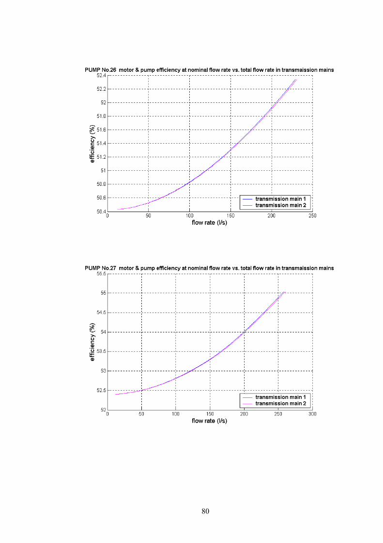
80

81

82

83

84

85
Appendix B: plots of power consumption against total flow rate in
transmission main 1 - for individual pumps (pumps No.2 and No.36 are
omitted due to unavailability of data)

86

87

88

89

90
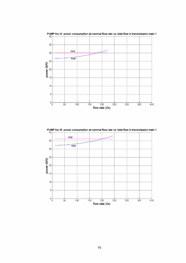
91
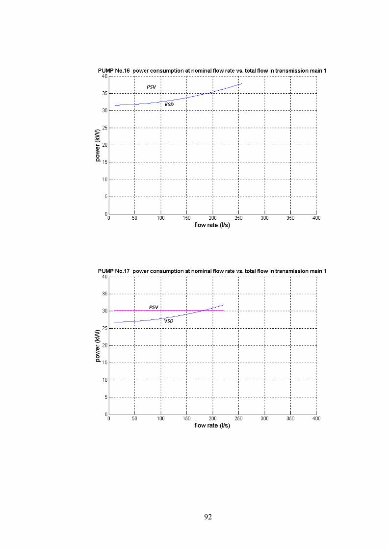
92

93

94

95

96

97

98

99

100

101