Can a Conditional Cash Transfer program change parents’

underlying behavioural parameters and hopes for their

children?∗

Diana Contreras Suarez†

September 2015

Abstract

While Conditional Cash Transfer programs have been designed to improve longterm human capital among poor families through incentives and conditions, we testif they change behaviour through changes in preferences and aspirations rather than,or in addition to, the effect of the conditions and incentives. Using the poverty scorefor program allocation we estimate the program effect on preferences and aspirationsusing a regression discontinuity (RD) design. We provide evidence of validity of theRD design through the density of the assignment function and comparison of covariatesat baseline. We find no evidence of changes in the program working through parentstime preferences or aspirations for their childrens schooling in participating households.On the contrary our results suggest that most likely those children will not finish highschool unless the program is operating. Thus, the positive program impacts identifiedin previous studies appear to be driven by the ongoing receipt of the cash transfersand the associated conditions. Thus if the program was to stop, we would expectinvestment in childrens human capital to revert to pre-program levels.

Key Words: Conditional Cash Transfer, Time preferences, Schooling aspirations,Regression Discontinuity Design

JEL Classification Codes: I25, I38, O15, D91

∗I am very grateful to my advisor Lisa Cameron for her invaluable support, discussions and encourage-ment. I thank the participants of the Australasian Development Economics Workshop for their comments,specially to Oriana Bandiera. I thank the Colombian National Planning Department, Econometria andthe Institute of Fiscal Studies for the information provided and for allowing me to participate in the longterm evaluation of the program Familias en Accion. All remaining errors are mine alone.†Department of Econometrics, Monash University, Clayton Campus, VIC 3800, Australia. Email:

Diana.Contreras.Suarez@monash.edu.

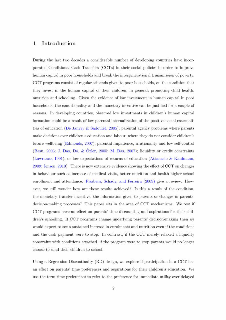
1 Introduction

During the last two decades a considerable number of developing countries have incor-

porated Conditional Cash Transfers (CCTs) in their social policies in order to improve

human capital in poor households and break the intergenerational transmission of poverty.

CCT programs consist of regular stipends given to poor households, on the condition that

they invest in the human capital of their children, in general, promoting child health,

nutrition and schooling. Given the evidence of low investment in human capital in poor

households, the conditionality and the monetary incentive can be justified for a couple of

reasons. In developing countries, observed low investments in children’s human capital

formation could be a result of low parental internalization of the positive social externali-

ties of education (De Janvry & Sadoulet, 2005); parental agency problems where parents

make decisions over children’s education and labour, where they do not consider children’s

future wellbeing (Edmonds, 2007); parental impatience, irrationality and low self-control

(Basu, 2003; J. Das, Do, & Ozler, 2005; M. Das, 2007); liquidity or credit constraints

(Lawrance, 1991); or low expectations of returns of education (Attanasio & Kaufmann,

2009; Jensen, 2010). There is now extensive evidence showing the effect of CCT on changes

in behaviour such as increase of medical visits, better nutrition and health higher school

enrollment and attendance. Fiszbein, Schady, and Ferreira (2009) give a review. How-

ever, we still wonder how are those results achieved? Is this a result of the condition,

the monetary transfer incentive, the information given to parents or changes in parents’

decision-making processes? This paper sits in the area of CCT mechanisms. We test if

CCT programs have an effect on parents’ time discounting and aspirations for their chil-

dren’s schooling. If CCT programs change underlying parents’ decision-making then we

would expect to see a sustained increase in enrolments and nutrition even if the conditions

and the cash payment were to stop. In contrast, if the CCT merely relaxed a liquidity

constraint with conditions attached, if the program were to stop parents would no longer

choose to send their children to school.

Using a Regression Discontinuity (RD) design, we explore if participation in a CCT has

an effect on parents’ time preferences and aspirations for their children’s education. We

use the term time preferences to refer to the preference for immediate utility over delayed

2

utility; high time preference is also referred to as impatience or a high discount rate. To

examine time preference and aspirations, we use information on hypothetical questions to

elicit the discount rate, the number of years of education parents would like their children

to complete and the probability parents place on their child completing each school level

(secondary and tertiary education).

Living in poverty is often associated with high time preferences and low educational as-

pirations (Bauer & Chytilova, 2010, 2013; Becker & Mulligan, 1997; Kirby et al., 2002;

Lawrance, 1991) mainly due to financial constraints, poor access to services and low levels

of education. These factors limit people’s ability to plan or invest, and to consider a wider

range of options for themselves and their children or delay gratification. Conditional Cash

Transfer programs offer people additional income and behavioural conditions. The income

transfer relaxes the budget constraint of the household, which once they are living above

subsistence levels creates the possibility for them to invest (in education or productive

activities, for example) and plan present-consumption versus future-consumption. The

budget relaxation can also increase the set of goods the households can afford, or create

demand for new items previously not considered. Even if the consumption of these goods

is only achievable with the new higher level of income, when income drops, the preference

(aspiration) for these goods may have changed due to the experienced access. If changes in

investments in human capital are due to relaxation of the budget constraint, the observed

effect of the program in changing behaviour will be temporary. In contrast, if preferences

have changed then the behaviour may change permanently.

Poor participant households have to take their children to the doctor, send their children

to school, and caregivers have to attend educational talks in order to receive the monetary

transfer. These conditions “force” them to change their behaviour. With time, they may

create the habit of actually delaying present gratification and increasing the act of investing

in human capital (L. Carvalho, Prina, & Sydnor, 2013). Additionally, the information

they receive in the educational talks may create awareness of the importance of education,

nutrition, health and general child care, making them change their preferences for human

capital investment. If they are meeting the requirements because of the budget constraint

relaxation, then the effect on their preferences for human capital investment for their

3

children will be temporary, but if they form the habit of investing (sending their children

to school or taking them to the doctor) and the new knowledge gained has changed their

preferences for human capital, then the preference for higher human capital investment

will be permanent.

Changing parents’ preferences could potentially have a double effect on boosting human

capital of children in poor households. If the program has an effect on parents’ underlying

preferences, parents will choose to keep investing in the human capital of their children,

even in the absence of the program or in addition to it. Additionally, these parame-

ters could potentially be transmitted generation to generation as the evidence suggests

(Dohmen, Falk, Huffman, & Sunde, 2012; Volland, 2013; Zilibotti & Doepke, 2014; Zum-

buehl, Dohmen, & Pfann, 2013). Although the focus of this paper is the effect of the

program on parents preferences and aspirations for their children, the program may have

an impact on childrens preferences (in addition to increasing their human capital). If

patience and aspirations are somehow learned by children from parents and they are also

associated with human capital investment decisions, changes in parents’ preferences would

have an impact not only on parents’ decisions over children’s schooling but also on chil-

dren’s own decisions. If children are more patient they may also, for example, aspire to

jobs with better wages after a period of training or education, as opposed to lower paying

jobs (Lawrance, 1991). They may also choose to invest more in their own children. This

effect could then potentially break the cycle of poverty.

2 Literature review

Understanding how underlying behavioural parameters are formed, what are the factors

they are associated to and how they evolve (if they do evolve), is important to predict and

evaluate public policies and institutional arrangements (Bowles, 1998). Changing some

parameters amongst poor households, like time preferences or educational aspirations, is

likely to boost human capital development. There are very few empirical studies examining

this in developing countries.

4

2.1 Time preferences

Time preferences seems to be to some extent learned from parents, change over the life time

and are very likely to be affected by social pressure and circumstances. The psychological

literature recognizes that humans are born impatient and later learn to be future oriented

and choose actions with postponed rewards (Mischel, Shoda, & Rodriguez, 1989). One

of the most early source of preferences variation is parental influence. Empirical evidence

exists of intergenerational transmission of behavioural preferences like work attitudes (Fer-

nandez & Fogli, 2009) or leisure activities (Volland, 2013); and underlying preferences like

risk and trust (Dohmen et al., 2012; Zumbuehl et al., 2013) or academic aspirations and

motivation (Benner & Mistry, 2007; Kirk, Lewis-Moss, Nilsen, & Colvin, 2011). Addi-

tionally, Doepke & Zilibotti (2008) and Zilibotti & Doepke (2014) provide a theoretical

framework where children’s preferences are learnt from parents, They show that even when

different parenting styles are considered in the model the result holds. These similarities

in preferences within families may partially explain substantial intergenerational persis-

tence of different economic outcomes like income, wealth and education (Bowles, Gintis,

& Groves, 2009).

Anderson, Dietz, Gordon, & Klawitter, (2004) argue that preferences are to some extent

biologically determined but not immutable as they are sublimated by parental teaching,

social pressure and circumstances, like permanent income or income shocks. For example

poverty has been associated with high time preferences and low educational aspirations.

They are also associated with low education, wealth and income, household composition,

gender and age (Bauer & Chytilova, 2010, 2013; Becker & Mulligan, 1997; Kirby et

al., 2002; Pennings & Garcia, 2005; Tanaka, Camerer, & Nguyen, 2006). Becker and

Mulligan (1997) argue that education can be an investment in patience. As individuals

grow older and their level of education increases, education can help them to form a

picture of life, its pleasures and difficulties. Constant practice of problem solving will also

enhance the process of anticipation as individuals learn the art of scenario simulation. In

that sense, education helps people to perceive future pleasures as less remote. However,

poor households are usually characterized by low education, income and wealth and tend to

be more impatient favouring present over future consumption. Over the total population,

5

Lawrance (1991) finds that poor households in the US have time preferences 5 percentage

points higher than richer households. Similarly, L. S. Carvalho (2010), using information

from rural Mexico finds that the poor seem to be very impatient. Women and older people

seem to be more patient. In the same line, Bauer and Chytilova (2013) also find that

women in Indian villages are more patient than men. Equally they find heterogeneity in

patience according to household composition, for example parents with younger children

are the ones who exhibit lower time preferences. Among the poor there is not clear

how income variation affect time preference. Using hypothetical information in Vietnam,

Anderson et al. (2004) find women more patient than men but no differences coming from

income variation. Rubalcava, Teruel, and Thomas (2009) indicate that Mexican women

are as well more patient than men when thinking about the future. But, they find that

additional income from cash transfers given to married women is more likely to be spent

on small livestock, improved nutrition, and child goods, which are more future-oriented

investments. Similarly, Dean and Sautmann (2014) find that changes in preferences are

related to changes in non-labour income rather than to labour income. This suggest that

control over income variation might play a role in changing time preferences.

2.2 Parents’ aspirations

Parents’ aspirations are consistently related to children’s ultimate school achievements

(Benner & Mistry, 2007; Chiapa, Garrido, & Prina, 2012; Spera, Wentzel, & Matto,

2009). Low levels of parents’ education, income and expected returns to education have

been shown to be associated with parents having low schooling aspirations for their children

(Attanasio & Kaufmann, 2014; Davis Kean, 2005; Halle, Kurtz-Costes, & Mahoney, 1997;

Sosu, 2014; Spera et al., 2009). While the economic literature on the relationship between

poverty and parental educational aspirations for children is still limited, the education and

psychology literature provides more information. Halle et al. (1997) using a sample of

low-income minority families in the US finds that mothers with high education had higher

aspirations for their children’s academic achievement. Even when parents’ expectations1

reflect parents’ aspirations adjusted by constraints to attain them, Davis Kean (2005)

1 Educational aspirations refer to the desired level of education (free of real world constraints) whileeducational expectations refer to the assessment of the real possible educational achievement of the child.

6

similarly finds using data from the US that parents’ education shapes their expectations

over children’s educational achievement. However ultimately the way these aspirations

are formed is unclear. A possible mechanism could be the beliefs of the decision makers

about the nature of private investment and their possible future returns. For example,

parents may believe that earnings respond to education less elastically than they actually

do, which may result in parents placing low value on schooling. Attanasio and Kaufmann

(2009) tested this hypothesis using data from Mexico and found that earnings obtained for

young adults between 15 and 25 years old are higher than the expected returns, especially

among children of parents with low education levels.

Household income can either enable or limit parents educational aspirations for their

children. The range of options individuals aspire to is influenced by the options they

can realistically contemplate. The options and opportunities (or lack of them) are usually

related to their own income and wealth as well as the income and wealth of their neighbours

or people with whom they interact. For example, comparing own standards of living or

achievements with neighbouring people can influence ones own aspirations (Appadurai,

2004; Ray, 2006). Overall, if age, household composition, income, wealth and interactions

with others are related to time preferences and aspirations and they adjust over time, then

preferences are likely to change to reflect current circumstances (Becker & Mulligan, 1997;

Bowles, 1998).

This paper contributes to the literature that examines how changes in circumstances such

as changes in income, knowledge of a wider range of options and changes in regular be-

haviour (sending children to school or taking them to the doctor) can potentially change

underlying behavioural parameters of individuals. We look in particular at time prefer-

ences and aspirations in education. Empirical evidence of their evolution is still limited

mainly due to lack of longitudinal studies. Kirby et al. (2002), using incentivized choices

of immediate or delayed gains collected information every three months for 2 years in a

sample of Tsimane’ Amerindians in 2 villages in rural Bolivia. They find that high time

preferences, high rate of consumption and impulsive behaviour, although relatively sta-

ble characteristics are also influenced by situational factors like income variation. Using

tax return information from individuals in Boston, Meier and Sprenger (2014) find that

7

discount parameters are stable over the period of 2 years. While the parameters over

time are far from perfectly correlated, the differences are uncorrelated with levels and

changes in socio-demographic variables. This evidence however is limited by the short

period of analysis, the particular population included and the small size of the changes

in the socio-demographic variables considered. Discount parameters may take longer and

require bigger changes to adjust and may depend on the initial conditions or context of the

individuals, like living in poverty or in developing countries. Dean and Sautmann (2014)

use panel data to evaluate the impact of a randomized trial for a health care program for

children in Mali. They find persistence in discount choices of about 69%. However, they

find that the marginal rate of intertemporal substitution varies systematically with in-

come, consumption, spending shocks and savings. For example, individuals increase their

discount rates right before pay-day or if they just have experienced an adverse shock. In

the same line Cameron and Shah (2015), using data on individuals in Indonesia show

that exposure to negative shocks such as natural disasters makes individuals exhibit more

risk-averse choices and changes their subjective beliefs (occurrence and severity of future

events). They cannot definitively show that risk preferences change (as distinct from

changes in beliefs about the state of the world) but they acknowledge that changes in the

underlying preferences is one possible cause of these changes.

Finally, availability, experience and knowledge of services or goods can change individuals’

preferences for them. For example availability of financial institutions and the habit of

making regular choices like saving can affect preferences for risk taking or experiencing

better health or education. Exposing people to these options could increase the preference

for education and health. L. Carvalho et al. (2013) provide evidence that the option of

opening a savings account and the act of saving, seems to increase risk attitudes and the

willingness to delay gratification among poor households in Nepal. Although they are

not able to distinguish whether the effect comes from increased wealth or a change in the

preference for saving, they state that access to savings accounts and saving itself could

change the marginal utility of consumption affecting present-bias choices. Additionally,

they find that access to savings accounts changes preferences towards considering broader

options. Chiapa et al. (2012) provide some similar empirical evidence in this line in terms

of parents’ educational aspirations over their children. Using information from Mexico they

8

find that a CCT that increases parents’ exposure to and interaction with more educated

individuals than themselves can explain, at least in the short term, an increase in parent’s

aspirations for their children’s education. Additional income and behavioural conditions

coming from the Familias en Accion program in Colombia are the potential channels

through which parents’ time preferences and aspirations for their children’s schooling can

change.

There is not much evidence of changes in parameters in the CCT literature. Using data

from an unconditional cash transfer in Kenya targeting households with one deceased or

chronically ill parent, Martorano, Handa, Halpern, and Thirumurthy (2014) do not find

differences in intertemporal choice of the parent or caregiver when comparing treatment

and control locations two years after exposure to the program. However, the identification

of this effect was not clear as, by the time of the evaluation, both treatment and control

locations were receiving the treatment. Chiapa et al. (2012) study changes in parents’

aspiration for their children’s years of education in the Mexican CCT. They find that in

the short-term Progresa is associated with an increase in educational aspirations of about

a third of a school year. They explain this positive effect from mandated exposure to

educated professionals (doctors and nurses).

The CCT program can have an effect on children’s preferences and aspirations aspirations

through other channels, not only via learning from their parents (Kirk et al., 2011; Zilibotti

& Doepke, 2014). Preferences may also change as a result of higher education attainment

and higher potential income resulting from the program’s conditions. There are at least

four potential channels for time preferences to be reduced if education is increased. First,

schooling may promote increased cognitive skills and the ability to simulate and plan for

the future (Becker & Mulligan, 1997). Second, education may allow individuals to develop

mechanisms to control present consumption such as savings and investment (Duflo, 2006).

Third, education might promote health and reduce mortality risk (Cutler & Lleras-Muney,

2010) and this would make individuals more willing to delay their spending. Finally,

more educated individuals may face fewer income constraints that allow them to live

above subsistence income levels lowering the pressure for present consumption (Bauer &

Chytilova, 2010).

9

3 The program

Colombia, following the trend of a large number of Latin-American countries, implemented

the program ‘Familias en Accion’, a Conditional Cash Transfer program in poor rural

areas from 2002. The overall aim of this initiative was the creation of human capital in

households experiencing extreme poverty through monthly transfer payments. Households

were classified as extremely poor if they belonged to the first quintile of a poverty index.

We will take advantage of this selection criterion for our identification strategy, assuming

that participation in the program is discontinuous at an exogenously defined cut-off on this

poverty index. The transfer was expected to improve the education levels via improved

school attendance, as well as improved health and nutrition of children via regular medical

check-ups in rural households. The transfer represented on average 16% to 25% of the

total monthly income of the household and was received by the caregivers.

The program included a health and nutrition component that was offered to households

with at least one child aged between 0 and 6. Each household received approximately

US$25 regardless of the number of children they had in the 0 to 6 years age bracket. This

transfer was conditional upon children attending growth and development check-ups every

two months, and a vaccination program. Primary caregivers2 needed to attend talks on

hygiene, diet and contraception. The program also included an educational component

that was offered to households with children aged between 7 and 17. The transfer was

approximately US$8 for each child in primary school, and US$16 for each child in secondary

school3. The monetary transfer was subject to an average school attendance rate of more

than 80% per child. In essence, the program consisted of a monetary transfer to the

caregiver, contingent on medical check-ups for children aged 0 to 6, school attendance

for children 7 to 17 and information sessions for caregivers. In those information sessions

topics like health care for children, nutrition, sanitation of the household, care of the

household members and contraception were discussed.

2 The caregivers are primarily the mother of the child receiving the benefit. In some cases the father, thegrandmother or other household members are the caregivers if the mother does not live in the household.This case represented around 6% of the households participating.

3 The Colombian school system is divided into five years of primary school followed by four years in basicsecondary and then two years of middle secondary school, for a total of six years of secondary education.After finishing secondary school, individuals can pursue vocational or tertiary education.

10

The program was originally offered only in some municipalities4 in the country. The se-

lection of municipalities was based on population and infrastructure characteristics. Mu-

nicipalities had to i) have a population of less than 100,000 and not be the principal town

of the state, ii) have enough health and education infrastructure, iii) have a bank branch,

and iv) the town government had to show interest in being part of the program as well

as completing the required documents and providing the identification numbers of the

possible beneficiaries of the program. As the aim of the program was to improve human

capital among the poorest families, the selection of households was based on the poverty

level and presence of children. A household was eligible if i) it was classified as poor by

the poverty index SISBEN, ii) it had at least one child aged 0 to 17 and iii) it lived in

a municipality where the program was going to operate (treatment municipalities). The

take-up rate of the program was over 90%.

The SISBEN index is the instrument designed by the government to rank households

and identify them as a target population for social expenditure. This index was first

constructed in 1999 as a proxy indicator5 of the resources of households according to their

life conditions with values between 0 and 100. Values close to 0 represented the poorest

households while those close to 100 the rich. The threshold imposed to be classified as

poor and participate in the program was different in rural and urban areas6.

The program became operational at the end of 2002 including 691 municipalities out of

1060 in Colombia. Household participation in the following ten years after the program

started was mainly defined by geographical location, the poverty index score and presence

of children aged 0 to 17 in the household. Due to success with respect to health, nutri-

tion and education outcomes achieved by the program, in 2007 it was extended to other

rural municipalities, indigenous populations, households who were internally displaced,

and urban municipalities of the country. The program grew from reaching about 320,000

households in 2002 to around 2.8 million in around 900 municipalities in 2010, making

4 Municipalities refer to the major governmental administrative units in Colombia5 This indicator is the first principal component of four factors of household characteristics including

education and social security; demographic characteristics and income; dwelling quality and equipment;and available utilities.

6In Urban areas households had to have a SISBEN score lower than 34 and in rural areas a score lowerthan 14.

11

Familias en Accion one of the biggest programs for poor households implemented by the

Colombian government.7

If preferences are highly stable over generations, this limits the role for public policy to im-

prove school attendance, attainment or other outcomes. However, programs such as school

vouchers or CCTs have shown that external incentives can either change parents’ schooling

decisions over their children’s education or help them to free up credit constraints and so

achieve previously unfeasible educational aspirations. We identify three potential channels

through with the program can affect time preferences and aspirations: the transfer; the

habit of sending children to school or taking them to medical check ups; and the infor-

mation provided to parents. The transfer, in addition to relaxing the budget constraint

of the household, provides the opportunity to plan and acquire a wider range of options

unachievable before. The habit of fulfilling the program conditions, imply that parents

are required to delay present consumption. Repeated exposure to this delay might create

the habit of delaying consumption or gratification and also change the utility function

by for those new consumed goods (health and education). For example, if a poor parent

not only has less ability, but also less willingness to invest in children’s human capital

formation even with public education provision (M. Das, 2007), a sustained cash transfer

and the habit of experiencing health care and schooling would expand parents’ schooling

choices and increase their aspirations for their children’s schooling. Finally, information

increase the set of possibilities that can be considered and also can change preferences and

aspirations via education (Becker & Mulligan, 1997). We expect that the habit of delaying

present consumption (sending children to school and taking them to medical centres) and

the information provided in the information sessions on general family care would not only

increase the range of possibilities available and experienced by parents but also change

their preferences towards them (they prefer them more).

There is evidence of changes in habits for this population. Familias en Accion has increased

the enrolment rate of children aged 14 to 17 by 5.6 percentage points (Attanasio et al.,

7Note that the SISBEN score is also used for targeting of subsidised health care and a childrens nurseryprogram. However, the childrens nursery program is targeted at younger children. Further, the thresholdfor subsidised health care is higher than that for Familias en Accion thus most families in our control andtreatment groups are likely to have access to subsidised health care (around 80%). Hence, we are confidentwe are identifying the impact of Familias en Accion on preferences, not the impact of overlapping programs.

12

2010), the probability of finishing high school in rural areas by 6 percentage points (Baez &

Camacho, 2011) and the number of children who have regular visits to medical check-ups

by around 28% (Attanasio, Battistin, Fitzsimons, & Vera-Hernandez, 2005).If the program

only affects the choices via a relaxation of the budget constraint or the choices are merely

a product of the conditions of receiving the money, it is likely that the effect on behaviour

would last only while the transfer is being received. In contrast, if the observed choices

come from a change in the preferences towards education and delayed consumption, the

effect of the program on preferences may be permanent. This change in preferences would

not only increase participants’ willingness to invest more in their children’s schooling, but

also in other important outcomes of human capital development such us health, nutrition,

mental stimulation and/or leisure.

4 Data and Methods

4.1 Data

The data used in this paper comes from a follow-up survey implemented in 2012, 10 years

after the program started. This survey provides our only data on the discount rates and

parents’ aspirations for their children’s schooling attainment. It also provides information

on socio-demographic characteristics of the households, and children’s schooling history.

We measure time preferences using a hypothetical set of four questions to elicit the implicit

discount rate. These questions are asked of only one adult per household (mostly the

household head or his/her spouse), where the person is faced with a choice of being paid a

hypothetical amount today or a larger sum in the future. Table 1 presents the four choices.

The first one is the possibility of choosing between 100,000 COP today and 105,000 COP in

a month. If the person chooses the 105,000 COP then the other options are not presented

but if the person chooses 100,000 COP then the second option is presented. The second

option offers 120,000 COP in a month (versus 100,000 COP today), the third option offers

150,000 COP and the fourth one 200,000 COP. The offering process continues until the

person switches from the present option to the future option or until the options are

exhausted. This procedure allows us to calculate five intervals of the monthly discount

13

rate. For example someone choosing 105,000 COP in a month rather than 100,000 COP

today exhibits a discount rate between 0 and 0.05 (most patient), but someone who did

not choose the 105,000 COP offer and switches when the second option is offered (120,000

COP in a month) exhibits a discount rate between 0.05 and 0.2 (less patient). Figure 1

shows the density distribution for our sample in our five intervals. We observe that for

this sample the most chosen option exhibits an underlying discount rate between 1 and∞

(associated with choosing 100,000 even when 200,000 is offered in a month’s time). The

average monthly household income in the sample at the time of the interview was 830,000

COP8. Hence, the amount offered ‘to be received today’ is about 12% of average monthly

income.

A low discount rate represents a low preference for present consumption and we will refer

to this interchangeably as low time preferences or more patience. We will use a midpoint

of the interval as our best estimate of the person’s discount rate, similar to the strategy

used by Bauer and Chytilova (2010). Someone who exhibits a discount rate between 0 and

0.05 will be associated with a discount rate of 0.025. We will have 5 possible underlying

discount rates: 0.025, 0.125, 0.350, 0.75 and 1. Note that given that the last interval is

open to the right (1 - ∞) we use for that case the lower value of the interval. This gives

us the lower bound of the real discount rate for this sample.

To measure parents’ aspirations for their children’s schooling, we use three indicators

reported only for the oldest child aged 6 to 17 in the household.9 This question is asked

of all the caregivers of that child, in most cases this is the parents. The first indicator is

their aspiration for the number of years of education this child will attain. We calculate

the number of years of education, combining the information on the believed highest level

of education the child will achieve and the number of years in that level10. For example, if

a parent indicates that he aspires for his child to reach the third year of secondary school,

then the aspirational number of years for education will be 8 years. In Colombia there are

8 Using an exchange rate of 1900, the average monthly household income is U$ 436.9Please note that we define aspirations in this context as the parents’ desire for their children education

without explicitly stating a community reference in the way Bernard, Dercon, Orkin, & Taffesse (2014)construct their measure of aspirations

10In Spanish the questions were “¿Cual cree usted que es el grado de educacion mas alto que alcanzarael menor?” and “¿Cual es la cantidad de anos que usted cree que el menor aprobara en ese nivel?”

14

five main levels: Preschool level which is not compulsory; Primary school level (5 years);

Secondary school (6 years) which includes Basic level (4 years) and Vocational level (2

years); and Superior level. Superior level refers to either technical (2 years), technological

(4 years) and university (5 years). For a person to have a complete secondary education,

that person must complete all the grades of primary, basic secondary and vocational for a

total of 11 years of education. People can only access the superior level upon completion

of secondary level. Traditionally, someone with a university degree has completed 16 years

of education.

The second and third indicators are the caregiver reported probability of the child com-

pleting secondary education by age 18 and superior education. The hypothetical questions

to elicit these probabilities come from the questions (i) By the time the child is 18 years

old what is the probability he/she will have completed secondary education?11 And at any

age (ii) What is the probability that he/she will graduate from superior education?12 For

example, the person may believe the probability the child has finished secondary education

by age 18 is 90% but the probability of finishing superior education is 40%.

Because time preferences were asked from the household head or his/her spouse in all

households while aspiration questions were asked from all the caregivers of the child in

households with school age children, we have a sample size of 3065 for time preferences

and 4000 for caregivers’ aspirations. The sample is also evenly distributed between urban

and rural areas. We disaggregate at this level because traditionally education demand

and supply is lower in rural areas and also because the eligibility criteria for participation

was different in urban and rural areas. We explain this in the next section. Table 2

presents descriptive statistics for our variables of interest. Panel A presents the descriptive

statistics for the discount rate. Around 40% of the sample has high time preferences, as

they always chose the 100,000 COP (values the present more), which is equivalent to

having a high discount rate. Only around 12% of the individuals selected the most patient

option (105,000 COP in the first offer). Individuals living in urban areas appear more

impatient than those living in rural ones. The mean monthly discount rate for the sample

11 In Spanish the question was “¿Que tan posible es que el menor, cuando tenga 18 anos, haya terminadoel bachillerato completo?”

12 In Spanish “¿Que tan posible es que el menor se gradue de educacion superior?”

15

is 0.62 which means that on average individuals are willing to give up $100 today if they

get $162 in one month.

Table 2 also reports the aspiration questions for all the child’s caregivers, which includes

parents as well as older siblings or other relatives in the household (Panel B)13; and also

presents it disaggregated for mothers (Panel C) and fathers (Panel D). We find that in

all groups the average number years of education aspired to for a child is about 13 years.

Fathers in urban areas have slightly higher average aspirations: just over 14 years. The

average probability that the child finishes secondary education by age 18 reported by care-

givers is 82% and the probability that they finish superior education is 65%. Aspirations

of people living in rural areas are consistently lower than for people living in urban areas.

If the program is affecting aspirations we might expect that mothers’ aspirations would

be higher than fathers’ given that they attend the educational talks and also primarily

received the monetary transfer; however we do not find a systematic pattern in the mean.

We believe that the information reported for aspirations represent aspirations and not

expectations. Using baseline data for the evaluation of the program we find that 43% of

individuals aged 12 to 30 did not complete primary education. If we look at the age 18 to

30 (by age 18, 67% of the individuals are no longer studying), we find that 53% of them

did not complete primary school in rural areas and 34% in urban areas. Figure 2 presents

the distribution of level achieved by cohort ages of 5 years from 1214 to 30. An increase in

the probability of completing secondary and tertiary education is an increase of the lined

and black areas that were very small particularly in rural regions. The average number of

years of education in rural areas for individuals 18 to 20 and 21 to 25 is 5.6 and 5.0 while

in urban areas it is 7.2 and 6.8. This indicates that on average people complete primary

school but do not go much further. Note that the aspirations reported in the survey by

far exceed actual educational attainment in these areas. Hence, they seem to reflect the

hopes of the parents and caregivers, and not necessarily the financial and other constraints

faced by these households.

13 Only around of 10% of the reporters are other people other than the father or mother of the child14 We restrict the starting point to 12 as by that age children are supposed to have finished primary

school.

16

4.2 Identification strategy

To identify the program effect on the variables of interest we use a Regression Discontinuity

(RD) design based on the household eligibility criteria of the presence of children 0 to 17

and the poverty score (SISBEN) for identification of participants in the program.

The control group is made of non-eligible households living in the municipalities where the

program was implemented in 2001 and where in the initial sample design for the evaluation

of the program. These additional households, although having children 0 to 17 and living

in municipalities were the program was going to operate, were not eligible because they

were just above the cut-off point of the poverty index for eligibility. The intuition for using

those households as control is that households who are just above the cut-off are similar

enough to those who are just below. This sample was selected from all the households

who were above the cut-off point in both rural and urban areas. The cut-off was different

in rural and urban areas and the bandwidth used for sampling was different as well. In

rural areas the cut-off point was at SISBEN score 14 and the bandwidth for sampling was

4. This means that the households of comparison are households between 10 and 18 in the

SISBEN index in rural areas. In urban areas the cut-off was established at the SISBEN

score of 34 and the bandwidth used was 6, which generates a sample of households with

SISBEN scores between 28 and 40.

The key point for this identification strategy is that the participation in the program is

determined at least partially by the poverty score lying at each side of the fixed cut-off

(Imbens & Lemieux, 2008). Eligibility in essence is determined by the poverty score and

the cut-off, thus we expect to find a discontinuity in program participation at the cut-off

point. For the analysis hereafter we centre the score to 0 where negative scores represent

eligibility while positive ones represent ineligibility. Centring the score to zero allows us

to make a combined analysis of the total sample as the cut-off point for eligibility was

different in rural and urban areas. However, as urban and rural areas differ in a variety

of ways, we also break down the sample by urban/rural in the analysis.

This setup gives us a sample of around 880 individuals with poverty scores above the

17

cut-off (ineligibles) and 2800 below the cut-off who are eligible individuals. Table 3 shows

the number of observations of eligible and ineligible households of the variables of interest.

Please note that to allow us to focus on the area around the cut-off, all the visual in-

spections will be truncated to the poverty score interval [-4, 4] hereafter. The full sample

however, goes from -14 to 4 for rural areas and -34 to 6 in urban areas. Figure 3 presents

the distribution of the poverty score for this sample.

Graphically, we can see a jump in the probability of participation around the cut-off point

(poverty score equal zero) for both samples, time preferences and caregivers’ educational

aspirations for the children (see Figure 4). Comparing discount rates or educational as-

pirations for the children of individuals who were just above and below the cut-off point

eliminates selection and omitted variables bias and also allows us to estimate the causal

effect of the program at poverty score equal to zero that determines eligibility. Figure

5 presents the same jump in the probability of participation disaggregated by rural and

urban areas and figure 6 for mothers and fathers separately in the educational aspirations

sample. We include this break down for the education aspirations sample as the program

gave the transfer to the mother15 and they also attended educational talks, so mothers’

exposure to the program differs from fathers’.

5 Econometric framework

The Regression Discontinuity design takes advantage of the randomization given by the

discontinuous change in the probability of program enrolment with some continuous vari-

able (Z). The causal treatment effect on a potential outcome (Yi) can be obtained by

the difference between the outcome when exposed to the program Yi(1) and the outcome

without exposure to the program Yi(0). The traditional problem in causal inference is that

we do not observe both states at the same time. We only observe the outcome related to

the treatment received by the individual. If we define Di∈{0, 1} where (Di = 0) denotes

non-participation or (Di = 1) participation in the program, the outcome observed can be

described as

15The transfer is made to primary caregivers who are mostly mothers.

18

Yi = (1−Di)Yi (0) +DiYi (1) =

{Yi (0) if Di = 0Yi (1) if Di = 1

(1)

Additionally, we also observe pre-program covariates Zi and Xi. The main characteristic

of these covariates is that they are known and not affected by the program. The RD

design relies on the principle that the probability of participation in the treatment changes

discontinuously in the continuous covariate Zi, which means that individuals lying just

above a fixed threshold c are similar to those individuals that are just below, with the only

difference being that the former do not participate in the program while the latter do. Zi

could be itself associated with the potential outcomes but this association is assumed to

be smooth.

We can define the individual participation as16

Di (Zi) = I [Zi≤c] (2)

In the case of complete compliance, the value of Di is a deterministic function of Zi and the

probability of participation jumps from 0 to 1 at the threshold. If this is the case we could

use a sharp RD design. But this is not our case. Figure 4 shows that participation in the

program jumps from about 60% of households to above 90% of households at the poverty

score cut-off. Initial compliance was around 90% but with the change in the poverty score

around 35% of the households changed their eligibility status.

In the case of imperfect compliance -our case- a fuzzy RD design is used that allows for a

smaller jump in the probability of assignment to the treatment at the threshold17

limz↓c

Pr (Di = 1|Zi = z)6= limz↑c

Pr (Di = 1|Zi = z) (3)

Where limz↓c Pr (Di = 1|Zi = z) is the limit of the probability of participation when the

16 In our specification the poverty score Z is allocated at the household level and not by individual level17 A detailed explanation of RD design can be found in Imbens and Lemieux (2008) and Lee and Lemieux

(2010).

19

value of z gets closer to c from the right and limz↑c Pr (Di = 1|Zi = z) when z gets closer

to c from the left. In this case, following Hahn, Todd, and Van der Klaauw (2001), the

average causal effect of the treatment is obtained from the ratio of the discontinuity of the

outcome to the discontinuity of the participation at the eligibility threshold.

τ =limz↓cE (Y |Z = z)− limz↑cE (Y |Z = z)

limz↓cE (D|Z = z)− limz↑cE (D|Z = z)(4)

Interpreting τ as the average treatment effect when participation near the threshold is ran-

dom implies that the discontinuity in the conditional distribution of the outcome comes

from the discontinuity in the conditional distribution in the participation. This estimator

allows heterogeneous effects and then identifies a Local Average Treatment Effect (LATE)

evaluated at the cut-off for eligibility. The interpretation of this ratio as a causal effect

imposes monotonicity and excludability in the program participation function, as is men-

tioned in Imbens and Angrist (1994). As they suggest, a LATE should be estimated using

a 2SLS. In this case, ignoring the effect of eligibility on participation and estimating an

OLS equation of the outcome variable on the eligibility around the cut-off would generate

a biased estimator of the true treatment effect due to omitted variables and self-selection

into participation.

5.1 Estimation equation

Following Lemieux and Lee (2014) and Lee and Lemieux (2010), we estimate the treatment

effect in our fuzzy RD design using an IV methodology in a 2SLS estimation. We use

a flexible parametric model to estimate the effect of program participation Di on time

preferences or educational aspirations Yi instrumenting Di with a dummy for eligibility in

the program Ei. The probability of treatment is defined by

Prob (D = 1|Z = z) = γ + δE + gD(z − c) (5)

Where E = 1 [Z≤c] indicates the eligibility in the program as the poverty score is lower

than the eligibility threshold. We centre the poverty score Zi to zero and in that case c is

20

equal to zero. The function gD(z − c) indicates a flexible polynomial regression function

of order p that allows the slope to be different to the left (βl) and the right (βr) of the

threshold. The equations are then defined by

Yi = γ1 + τDi + Ei

P∑p=1

βlpZpi + (1− Ei)

P∑p=1

βrpZpi + εih (6)

Di = γ2 + δEi + Ei

P∑p=1

βlpZpi + (1− Ei)

P∑p=1

βrpZpi + vih (7)

The program causal effect is given by τ . We expect the program to reduce the time

preferences through relaxation of budget constraints and/or the habit of delaying present

consumption. That is, we expect τ to be negative (reduced discount). In contrast, we

expect the program to increase caregivers’ aspirations for the children’s education due

to the relaxation of the budget constraint, the habit of sending children to school and

attendance at information sessions by the main caregiver. In this case, we expect τ to be

positive.

We cluster the error terms in both equations at the household level to allow for het-

eroscedasticity and to account for the poverty score being calculated at the household

level defining eligibility and participation at that level. Although monotonicity is itself

not verifiable, it appears a sensible assumption. This implies that household participation

in the program is a monotonically decreasing function of the poverty score, where for ex-

ample households who choose to participate when they are ineligible would still choose to

participate if they became eligible. Additionally, being at either side of the cut-off point

does not have an impact on individuals’ discount rates or education aspirations for the

children except through participation in the program.

As the treatment effect is obtained by comparing conditional expectations of Yi when

approaching from the left and from the right to the cut-off, the correct specification of the

regression function is important. We use a cross-validation procedure suggested by Lee

and Lemieux (2010) based on the Akaike information criterion (AIC) for model selection.

Assuming that the empirical specification is the true functional form of the underlying

21

data, the LATE provides an efficient estimator of the treatment effect using individuals’

different distances from the discontinuity threshold.

6 Results

This section presents the results in three parts. We first present the result of the first

stage and the selection of the polynomial order. Then we present the estimated causal

treatment effect of the second stage and finally some tests of the econometric specification.

The analysis will be presented for the total sample and also disaggregated by urban and

rural regions and for the educational aspirations by mother/father18.

6.1 Effect of eligibility on program participation

In figure 4 we observed a discontinuity of about 35% in the probability of participation in

Familias en Accion at the eligibility poverty score cut-off for the time preference sample

and also the adults’ aspirations sample. This jump is a necessary condition to be able to

estimate the causal treatment effect on our outcomes of interest. Table 4 and table 5 show

the size of the discontinuities in the probability of participation varying the polynomial

order. This is the first stage δ value of eligibility on participation in equation (7). We use

a cross-validation procedure suggested by Lee and Lemieux (2010) based on the Akaike

information criterion (AIC) for model selection. The preferred specification is the one

with the lowest AIC. In most cases the preferred specification has the same polynomial

order at both sides of the cut-off; however we allow for flexibility in the model by also

estimating different polynomial orders at each side of the cut-off and present these results

if that is the preferred specification. For example, in table 4 we found that the preferred

specification for the aggregated sample is a first order polynomial at both sides of the

cut-off. This result suggests that program eligibility is associated with an increase of 47%

in the probability of participation in Familias en Accion. For those living in rural or urban

18 This is for the sample of parents that we could match with the characteristics of the child for whomthe aspirations were reported.

22

areas the probability is 44% and 51% respectively19. The parameter is in all cases strongly

significant.

These magnitudes are comparable to the ones estimated for the educational aspirations

sample. The best fit for the first stage of caregivers’ aspirational years of education for

their children is mostly a first order polynomial except for the aggregated sample, where

a quadratic functional form is preferred. For mothers, we found that the best fit is a

first order polynomial for the sample that is on the left of the cut-off and a second order

polynomial for the sample on the right. When looking at the first stage for the other

outcomes of interest the results are very similar.

We present the first stage estimates for different polynomial order specifications and even

though the size of the effect decreases as the polynomial order increases; it is still similar

and significant at the 1% significance level. This gives confidence in the strength of the

first stage and the power of the eligibility at the cut-off point as an instrument.

6.2 Effect of program participation on Time preferences and Educa-tional aspirations

Using the preferred polynomial order, Figures 7 - 9 present the discontinuity in the ex-

pected value of time preferences and education expectations at the threshold for eligibility.

Using a binwidth of 0.05, the estimated line of the conditional expectation helps us to visu-

alize the identification strategy. The time preferences representation suggests two things.

The first and most important one is that there is no evident jump in the discount rate

from the left to the right of the threshold for eligibility. This suggests no program effect on

time preferences. The second is that we expected the slope of the line to be negative as it

is suggested in the literature that wealth and income are related to lower time preferences.

It seems that in the overall sample we find this pattern but to the left of the eligibility

threshold the line has a slightly positive slope.

For educational aspirations, we expect that as the poverty score increases (less poor) the

19 This is a weighted probability (weighted by the distance from the threshold) and so differs from theunweighted probability shown in the figures.

23

aspiration increases, giving a positive slope. We do see a jump at the threshold for the years

of education the caregivers aspire the child to attend and the probability of completing

higher education; however these jumps are in the opposite of the anticipated direction.

This result, if significant, would suggest that program participation is having a negative

effect on those aspirations.

The IV (2SLS) estimation of the causal effect parameters of program participation on time

preferences and education expectations is presented in Table 6. For time preferences, a

negative sign on the coefficient suggests a decrease in the time preferences (more patient

individuals) due to participation in the program; our results show that this is the case

for the whole sample both in rural and urban areas. However, none of these coefficients

are statistically significant. The hypothesis is that a sustained increase in income as

well as the habit of delaying present consumption (act of investing in children’s health

and education) could potentially change individuals’ underlying preferences and reduce

their impatience. The biggest reduction of around 0.04 in the discount factor was found

among urban households (a 6.25% decrease in impatience) but this is insignificant. These

findings are consistent with the null effect for this sample found in figure 7. This suggests

no program participation effect on time preferences. In figures 8 and 9 we present the

continuity/discontinuity in urban and rural areas.

The results for caregivers’ aspirations for their child’s education are more surprising. A

common assumption is that children do not go to school due to monetary constraints or

because long term investments (e.g. child education) are not highly valued. The pro-

gram seems to relax budget constraints, incentivise attendance at school among children

as a result of the conditionality, and provide information to the main caregiver about the

importance of education (Attanasio, Fitzsimons, & Gomez, 2005; Attanasio & Mesnard,

2006). Our hypothesis is that those factors may in turn lead to increased educational

aspirations for children, especially among mothers given that they are the ones receiv-

ing the transfer and attending educational talks. We however find very little effect on

educational aspirations. There is no significant effect across the whole sample. We find

a marginally significant negative effect among individuals living in urban areas and for

fathers (expecting around 1 year less, and significant at the 10% level).

24

Program participation is found to not have a significant effect on the reported probability

of finishing secondary school by the age of 18. Most of the coefficients are negative and in

all cases the standard deviation is large. The effect in rural areas is the only case where

the coefficient on program participation is positive but it is also insignificant.

The only significant program effect is for the probability of finishing higher education,

however the coefficient in this case is negative. This suggests that participating in the

program is associated with a 14.3 pp decrease in the perceived probability of finishing

higher education. While non-participating caregivers on average attach a 76% probability

to their children completing higher education, participating caregivers on average report

a probability of 62%. We find a larger negative effect for urban areas, females and women

significant at 1%. This result is consistent with the lower expected years of education

found before.

The program effect on caregivers’ expectations for their children’s education was to lower

the probability of children completing tertiary education. This is the opposite of what was

expected. This could be because they come to see their children’s schooling attainment

as being associated with program support, but when this is no longer available (after

secondary schooling) they attach a lower probability to being able to continue than those

households who are not exposed to the program. In addition to this, if children were

behind in school progression when they started to participate in the program (were old

for their school year); parents might reason that they would be unable to complete high

school while eligible for participation (under the age of 17). Similarly, this reasoning would

reduce the expected probability of graduating from tertiary education. It is very likely

that these results are revealing that those children will probably not finish high school

unless the program is operating.

In summary, we find no evidence that time preferences change with exposure to the pro-

gram. We also find no effect on the aspirations of parents or caregivers for their children’s

education measured by years of schooling and the probability of finishing secondary school.

We find, however, a negative program effect on the probability that children will finish

higher education. Thus it appears that the program effect depends largely on the ongoing

25

receipt of the cash transfer and associated constraints.

6.3 Specification Tests

6.3.1 Polynomial order

The accuracy of the estimation in the RD design is based on the correct polynomial order

specification of the true functional form of the underlying data used. As a sensitivity

test, we evaluate our results using the second-best specification according to the AIC20.

Table 7 shows these results. For time preferences we find larger coefficients but they

are still insignificant. The overall conclusion remains for expected years of education

and probability of finishing tertiary education, although the parameters seem to be less

precisely estimated using a higher order polynomial order.

6.3.2 Covariates

The inclusion of additional covariates besides the poverty score in the RD design estimation

can be used to eliminate sample biases present in the basic specification, help to establish

the validity of the RD design and improve precision (Imbens & Lemieux, 2008; Lee &

Lemieux, 2010). A general challenge for the probabilities of finishing school levels is that

standard errors are very high. For those variables including covariates in the estimations,

may be particularly useful. We include as covariates the gender, age, years of education

and the region (rural or urban) of the respondent. Table 8 presents the results for each

outcome and the coefficient of the first stage of eligibility on participation. We find that

the first stage in all the cases continues to be as robust as before.

In the time preference estimations, we do not find that age or education are associated

with time preferences. This may be a consequence of the low variation in the sample as the

population is poor, education is low and the age of household heads/spouses is similar.

20 We additionally calculate the BIC selection criteria. As both criteria are sensitive to the numberof observations and the number of parameters estimated, the AIC tends to select models with fewerparameters while BIC tends to select models with more parameters. In our case we find that in 60% ofthe cases they selected the same best-fit polynomial order.

26

Some studies suggest that low wealth, low education and unemployment are related to

high time preferences (Bauer & Chytilova, 2010; Kirby et al., 2002). We find individuals

living in urban zones exhibit less patience while females are consistently more patient as

is suggested in the literature. Across the different subsamples, the initial negative non-

significant result on time preferences holds. If time preferences are a stable parameter,

then this is not a surprising result. Dean & Sautmann, (2014) show that time preferences

look to be relatively invariant to changes in income, education and labour status; while

they are more responsive to adverse shock events.

When looking at caregivers’ aspirations for their children we find, as expected, that the

role of parents’ own years of education seems to be very important in the three indicators

reported. For example, one additional year of a mother’s education increases the expected

probability of their children finishing secondary and tertiary education by 1.7 and 2.4

percentage points respectively. These magnitudes are smaller for fathers but still positive

and significant. The aspirations are on average higher when looking at the urban sample.

The coefficient is particularly high for the probability of finishing higher education where

it is more likely that that level is offered. Finally, the age and gender of the respondent are

not consistently a predictor. The significant negative effect on the aspirations of children’s

years of education for fathers and individuals living in urban areas disappears once we

control for reporters’ characteristics. For the probability of finishing tertiary education,

we find that the program effect is of a smaller magnitude but still negative and statistically

significant for exactly the same sub-samples. We do not find any effect on the probability

of finishing secondary school but in this case all the coefficients are positive.

In table 9 we present the estimation of the basic model but now including covariates of

children’s characteristics like gender, school progression, age of enrolment and attendance

at nursery for the sample of parents21. Being a female or currently attending school are

children’s characteristics positively associated with parents’ aspirations, while the number

of grades repeated is negatively related22. Overall, higher school performance is associated

21 This sample contains only mothers or fathers reporting information on educational aspirations fortheir child.

22 As program participation is defined by present or past participation, not all the households classifiedas participating have children attending school. We however find that from the households that are notcurrently participating, around 50% are not because they did not meet the attendance condition.

27

with higher parents’ aspirations.

7 Internal validity and Robustness Test

The validity of the RD design is based on the assumption that eligibility in the program is

determined exogenously (Imbens & Lemieux, 2008). In our case this is given by the exo-

geneity of the poverty index and the threshold for eligibility. This implies that individuals

to the left of the cut-off for eligibility are similar to individuals to the right and also that

the poverty index is continuous at the cut-off.

This section first presents a visual test of the continuity of the poverty index at the cut-off

following the procedure proposed by McCrary (2008). Second, we present some evidence

of local balance of baseline variables on both sides of the cut-off. We test internal validity

at the household level as the poverty score and participation was defined at that level. We

also disaggregate by rural and urban areas as the cut-off point for eligibility was different

as explained in the data section. Finally, it is possible that time preferences are affected

by the receipt of the cash transfer during the period in which the transfer is received, but

revert to the original preferences once the cash transfer is no longer received. To examine

this, we present a robustness test where we compare the results for time preferences for

those currently receiving the cash transfer with those who had received the cash transfer

in the past.

7.1 Continuity in the poverty score

If individuals or households are able to manipulate the poverty score they receive in order

to become eligible to participate in the program, the RD design will not be valid as the

assignment would not be locally random. We first test using a visual inspection of the

continuity on the density of the poverty score and second, we treat the frequency counts

as a dependent variable in a local linear regression. Continuity in the poverty score at the

threshold is evidence of absence of manipulation. For the first test, we divide the poverty

score into equally spaced bins and calculate the frequency in each of them. Figure 10

28

shows the density of the poverty score for the time preferences and education aspirations

samples. While the density is continuous at the threshold for eligibility in the time pref-

erences sample, indicating no manipulability in the poverty classification, there is a small

discontinuity in the education aspirations sample. In Figure 11 we present the density for

this sample disaggregating by rural and urban region. We find that there is continuity in

the density distribution in rural areas but there is some evidence of discontinuity in urban

areas.

To test if there is continuity in the frequency counts at the threshold, we also present the

estimation of a local linear regression23 in Table 10, as suggested by McCrary (2008). We

find that the difference in the number of respondents is not statistically different above

and below the cut-off for eligibility in the aggregate or in rural or urban areas. However,

we find that on average there are two additional counts in the bins that are closer to

the cut-off on the left (eligible households) in the sample of education aspirations for the

aggregate. This seems to be driven by households living in urban areas.

This finding could however be consistent with a household composition change rather

than manipulation of the poverty score. While all households reported information on

time preferences, education aspiration questions were only asked of households who had

at least one child aged 6 to 17. More households qualifying to report information on

aspirations may reflect that children stay at home longer in participating households as

a result of the program. To examine this further, in Table 11 panel A we present some

results on household composition. We find no difference in the number of caregivers or

the proportion of females in the household (potential caregivers). We however find some

difference in the household composition that determines the number of households who

answer the educational aspiration questions. Those questions were answered by all the

caregivers in households with children 6 to 17 and referring to the oldest child in that age

interval. We find that the number of children 6 to 17 is higher in the aggregated sample

while not statistically significant when disaggregated by rural and urban area. When

looking at the number of children aged 12 to 17 which are the most likely group to contain

the child for whom the information is provided, we find that participant households in

23 We estimate an OLS model using the counts in bins of size 0.05 from -1.5 to 1.5 in the poverty score.

29

urban areas have on average 0.5 more children than non-participant ones. This difference

is significant at the 10% level. Other group ages seem to be similar. This finding is

consistent with the fact that there is a discontinuity in the counts density function in

urban areas. If participant households in urban areas are more likely to have children

12 to 17 then we expect to have more households to the left of the eligibility cut-off.

Thus, those differences in counts do not come from manipulation of the poverty score

but from changes in demographic composition resulting from the program. It seems that

older children of eligible households are deciding to remain in the households to guarantee

households’ eligibility for the program. This result is in line with the program aim to

increase school enrolment and attendance of older children, who are usually at risk of

dropping out of school.

In summary, given that when for the time preferences sample (all households) we find the

distribution is continuous, we are confident that manipulation was not occurring.

7.2 Baseline covariates

An important assumption in order to identify the program effect is that individuals to the

left and right of the cut-off were identical before the program started and that participation

in the program was random around the poverty score cut-off. To empirically test this

we would expect to find no discontinuities at the cut-off for covariates, except program

eligibility, before the program started. Unfortunately, we do not have information at the

baseline for individuals above the cut-off.

Comparing covariates at the end line could simply reflect program effect on the covariates.

We examine the local balance on either side of the threshold for eligibility using variables

that we consider unlikely to have been affected by the program. We use age and level of

education of the household head.

If the RD design is valid, we should find that characteristics of the household head are

continuous at the threshold. We present these results in Table 11 panel B. We find no

significant differences in age or education24 for the household heads of participant and non-

24 Adults in this population are very unlikely to reenrol at school. As shown, the probability of being

30

participant households living in urban and rural areas. When looking at the aggregate

result, the coefficient on education is different than zero but this is mainly driven by

educational differences between rural and urban household’s heads. This means that we

need to control for differences in education when analysing the aggregated sample. These

results were presented in the covariates section. We interpret this as evidence of RD

design validity, as households at the threshold were similar at the baseline over those

characteristics.

7.3 Time preferences and current income transfer

The final robustness test we conduct examines whether time preferences are affected by

the current receipt of the conditional cash transfer. As eligibility is defined by the poverty

score, the treatment group contains households who were participating in the program at

the time of the interview and also those who had participated in the past. Additional

income diminishes the pressure for present consumption and allows households to delay

consumption and plan better (Becker & Mulligan, 1997; L. S. Carvalho, 2010; Kirby et

al., 2002; Tanaka et al., 2006). If this is the most important component, disaggregating

the sample, we may find an effect on current participants’ time preferences. But this does

not apply in households that participated in the program in the past but are no longer

receiving the extra income.

We separate the sample into two subsamples of households who were participating at the

time of the interview (current participants) and households who had participated in the

program but are no longer participating because there are no longer children aged 0 to 17

in the household (past participants) and estimate the coefficients again for each sample.

If we find an effect on time preferences for the current participants, it may suggest that

the relaxation of the budget constraint is the main mechanism to affect the discount rate

for this sample. The results are presented in table 12. The effects are insignificant in

both samples. This suggests that even current receipt of the transfer is not affecting time

preferences.

enrolled at school by age 21 is very small.

31

8 Conclusions

We conclude that the program does not change participants’ time preferences and we find

no positive effects of the program on caregivers’ aspirations for their children’s education.

However, we systematically find that participating parents attach a lower probability to

their children finishing higher education. These results suggest that participant house-

holds’ motivation for sending their children to school is related to the monetary transfer

they received rather than to changes in preferences and aspirations. Observed changes in

behaviour and choices are thus a consequence of the incentive and conditions.

One possible conclusion is that time preferences and aspirations are largely fixed. Although

there is growing evidence that preferences do respond to negative shocks (Cameron & Shah,

Forthcoming; Dean & Sautmann, 2014), there is little evidence on the effect of positive

shocks.

If the program changes the preferences and hopes of participant households, from a pub-

lic policy perspective this would mean that temporary exposure to the program would

enhance future human development investment in children. However, we do not find evi-

dence that participants’ preferences or hopes of educational attainment for their children

increase. This suggests that if the program were to stop or the budget run out, the

program is unlikely to have long term effects on parents’ investment in the educational

attainment and health of the household. This however, does not imply that the program is

not effective overall as it has been shown in Attanasio, Battistin, et al. (2005), Attanasio

et al. (2010), Baez and Camacho (2011) and Attanasio, Battistin, and Mesnard (2012)

to improve children’s health status and educational attendance. It is possible that these

increases in education may increase children’s own time preferences and increase their own

educational aspirations even if their parents’ preferences remain the same. This is an area

for future research.

9 Tables

32

Table 1: Hypothetical time preference questions

Today Later Period discount rate Time preference

1 100000 105000 1 month 0.05 high (most patient)2 100000 120000 1 month 0.23 100000 150000 1 month 0.54 100000 200000 1 month 1 low (most impatient)

Table 2: Frequency of Interval of discount rate in per-centages and adults’ aspirations for child’s education

Total Rural Urban

Panel A: Discount rate Intervala

0 - 0.05 0.12 0.13 0.110.05 - 0.2 0.11 0.12 0.10.2 - 0.5 0.19 0.19 0.190.5 - 1 0.18 0.17 0.191 - ∞ 0.4 0.39 0.41

N 3065 1603 1462

Non-eligible Mean 0.62 0.60 0.64

Panel B: Caregivers’ Aspirations for the childrenb

Aspired years of education 13.47 13.11 13.86N 4095 2132 1963Non-eligible Mean 13.95 13.54 14.5Probability of finishing secondary school 81.44 79.95 83.03N 3945 2036 1909Non-eligible Mean 84.5 82.11 87.74Probability of finishing higher education 64.81 60.53 69.36N 3877 2000 1877Non-eligible Mean 69.11 64 76.13

Panel C: Mothers’ Aspirations for their children

Aspired years of education 13.42 13.1 13.77N 2548 1339 1209Non-eligible Mean 13.36 12.8 13.94Probability of finishing secondary school 80.97 79.35 82.73N 2460 1283 1177Non-eligible Mean 81.5 80.05 82.94Probability of finishing higher education 64.84 61.02 69.01N 2417 1262 1155Non-eligible Mean 61.54 56.34 66.87

Panel D: Fathers’ Aspirations for their children

Aspired years of education 13.52 13.05 14.06N 1089 582 507Non-eligible Mean 13.25 12.98 13.58Probability of finishing secondary school 82.52 80.87 84.37N 1046 552 494Non-eligible Mean 79.91 78.4 81.46Probability of finishing higher education 63.6 58.55 69.21N 1029 542 487Non-eligible Mean 63.51 59.75 67.38

a Results from hypothetical questions asked to one member of thehousehold.b Caregivers include any adult of the household including older sib-lings.Notes: In around 90% of the cases the caregivers are the parents.

33

Table 3: Sample by eligibility criteria and variables of interest

Score around the eligibility cut-offabove below

Discount rate 890 2175Expected years of education 907 3188Probability of finishing secondary school 877 3068Probability of finishing higher education 864 3013

Notes: Above include all individuals who have a poverty score above the cut-offpoint in the interval (cut-off value, ≈+5]. Below the cut-off includes individuals whohave a poverty score in the interval [0, cut-off value]. For both cases, the counts areof individuals in rural or urban areas that reported the variable of interest.

34

Table 4: Discontinuity estimates of program participation atpoverty score eligibility cut-off for Time Preferences sample

Polynomial order on both sides All Rural Urbanof the eligibility cut-off

1 0.4732*** a 0.4438*** a 0.5082*** a

(0.0219) (0.0296) (0.0338)2 0.4526*** 0.4256*** 0.4892***

(0.0310) (0.0424) (0.0488)3 0.3973*** 0.3756*** 0.4307***

(0.0383) (0.0556) (0.0603)4 0.3380*** 0.3349*** 0.3529***

(0.0451) (0.0663) (0.0714)5 0.3212*** 0.2937*** 0.3324***

(0.0511) (0.0769) (0.0827)Number of observations 3,065 1,603 1,462

Notes: The estimates come from the first stage estimation of the IV esti-mation. We calculated increasing polynomial level to the left and right bya unit, same polynomial order at both sides are presented. Household clus-tered standard errors in parentheses.a This is the preferred specification of the polynomial order based on theAIC criterion.Significance: *** p< 0.01, ** p< 0.05, * p< 0.1.

35

Table 5: Discontinuity estimates of program participation at poverty score eligibilitycut-off for educational aspirations sample

Polynomial order on both sides All Rural Urban Mothers Fathersof the eligibility cut-off

Panel A: Years of education

1 0.4278*** 0.4296*** a 0.4393*** a 0.4173*** 0.4886*** a

(0.0249) (0.0348) (0.0375) (0.0260) (0.0446)1 left, 2 right 0.4233*** 0.4047*** 0.4324*** 0.4151*** a 0.4989***

(0.0257) (0.0366) (0.0388) (0.0270) (0.0452)2 0.4378*** a 0.4322*** 0.4412*** 0.4239*** 0.5123***

(0.0332) (0.0475) (0.0500) (0.0347) (0.0593)3 0.4048*** 0.4430*** 0.3853*** 0.3935*** 0.4471***

(0.0420) (0.0618) (0.0651) (0.0436) (0.0783)4 0.3706*** 0.4149*** 0.3087*** 0.3498*** 0.4155***

(0.0504) (0.0708) (0.0804) (0.0517) (0.0938)5 0.3641*** 0.3851*** 0.3052*** 0.3443*** 0.4303***

(0.0564) (0.0805) (0.0942) (0.0574) (0.1124)Number of observations 4,095 2,132 1,963 2,548 1,089Panel B: Probability of finishing secondary school

1 0.4302*** a 0.4256*** a 0.4483*** 0.4169*** a 0.4926*** a

(0.0251) (0.0349) (0.0378) (0.0263) (0.0453)2 0.4446*** 0.4291*** 0.4607*** a 0.4280*** 0.5186***

(0.0333) (0.0478) (0.0498) (0.0351) (0.0601)3 0.4145*** 0.4367*** 0.4131*** 0.4003*** 0.4550***

(0.0422) (0.0625) (0.0649) (0.0442) (0.0798)4 0.3822*** 0.4163*** 0.3400*** 0.3588*** 0.4281***

(0.0507) (0.0721) (0.0803) (0.0527) (0.0958)5 0.3768*** 0.3965*** 0.3336*** 0.3553*** 0.4543***

(0.0569) (0.0819) (0.0938) (0.0585) (0.1151)Number of observations 3,945 2,036 1,909 2,460 1,046Panel C: Probability of finishing higher education

1 0.4312*** 0.4253*** 0.4514*** a 0.4177*** a 0.4976***(0.0252) (0.0350) (0.0381) (0.0265) (0.0454)

2 0.4444*** a 0.4277*** a 0.4628*** 0.4289*** 0.5200*** a

(0.0335) (0.0479) (0.0504) (0.0354) (0.0608)3 0.4140*** 0.4355*** 0.4153*** 0.4026*** 0.4545***

(0.0426) (0.0630) (0.0660) (0.0448) (0.0803)4 0.3839*** 0.4135*** 0.3505*** 0.3651*** 0.4322***

(0.0511) (0.0727) (0.0808) (0.0532) (0.0964)5 0.3815*** 0.3965*** 0.3496*** 0.3649*** 0.4573***

(0.0573) (0.0827) (0.0943) (0.0592) (0.1152)Number of observations 3,877 2,000 1,877 2,417 1,029

Notes: The estimates come from the first stage estimation of the IV estimation. We calculated increasingpolynomial level to the left and right by a unit, same polynomial order at both sides are presented.Household clustered standard errors in parentheses.a This is the preferred specification of the polynomial order based on the AIC criterion.Significance: *** p< 0.01, ** p< 0.05, * p< 0.1.

36

Table 6: Effect of Program Participation on Time Preferences and Education Aspira-tions

All Rural Urban Mothers Fathers

Time preferences

Discount rate -0.0148 -0.0252 -0.0355 NA NA(0.0450) (0.0705) (0.0579) NA NA

Number of observations 3,065 1,603 1,462

Education Aspirations

Years of education -0.5775 -0.5272 -0.9701* -0.5172 -1.1329*(0.5828) (0.6415) (0.5554) (0.5615) (0.6850)

Number of observations 4,095 2,132 1,963 2,548 1,089

Probability of finishing secondary school -2.9927 4.1882 -9.9530 -5.3741 -2.2762(3.8790) (5.4902) (6.2391) (4.7487) (5.9548)

Number of observations 3,945 2,036 1,909 2,460 1,046

Probability of finishing higher education -14.2513** -11.1006 -17.8300*** -17.1438*** -11.1198(6.2775) (9.9204) (6.1064) (5.6964) (9.1037)

Number of observations 3,877 2,000 1,877 2,417 1,029

Notes: This table includes the second stage of the IV estimation that gives the values of τ that is interpretedas a LATE estimator. The estimations include the number of polynomials at each side of the threshold foundto be of best fit using the AIC criterion.The estimations do not include covariates. Household clusteredstandard errors in parentheses.Significance: *** p< 0.01, ** p< 0.05, * p< 0.1.

37

Table 7: Program effect on Time Preferences and Education Aspirations in the second-bestpolynomial order

All Rural Urban Mothers Fathers

Time preferences

Discount rate -0.0676 -0.0984 -0.0722 NA NA(0.0642) (0.1008) (0.0849) NA NA

Eligibility on participation coefficient 0.4526*** 0.4256*** 0.4892***(0.0310) (0.0424) (0.0488)

Education Aspirations

Years of education -0.9167** 0.1665 -1.2369 -0.1784 -0.9244(0.4321) (0.9231) (0.9756) (0.6590) (0.9034)

Eligibility on participation coefficient 0.4278*** 0.4322*** 0.3853*** 0.4239*** 0.5123***(0.0249) (0.0475) (0.0651) (0.0347) (0.0593)

Probability of finishing secondary school 3.2808 1.5086 -7.1427 -0.1473 4.0670(5.0833) (7.8978) (5.3911) (6.0377) (7.4791)

Eligibility on participation coefficient 0.4446*** 0.4291*** 0.4483*** 0.4280*** 0.5186***(0.0333) (0.0478) (0.0378) (0.0351) (0.0601)

Probability of finishing higher education -16.3150*** -17.2148** -22.2868*** -19.6008*** -23.8279***(4.9642) (7.8315) (8.1820) (7.4526) (8.0233)

Eligibility on participation coefficient 0.4312*** 0.4253*** 0.4628*** 0.4289*** 0.4976***(0.0252) (0.0350) (0.0504) (0.0354) (0.0454)

Notes: This table includes the second stage of the IV estimation that gives the values of τ that is interpretedas a LATE estimator. The eligibility on participation is the first-stage parameter δ. The estimations include thenumber of polynomials at each side of the threshold found to be the second best fit using the AIC criterion.Theestimations do not include covariates. Household clustered standard errors in parentheses.Significance: *** p< 0.01, ** p< 0.05, * p< 0.1.

38

Table 8: Program effect on Time Preferences and Education Aspirations in-cluding covariates

All Rural Urban Mothers Fathers

Time preferences

Discount rate -0.0136 -0.0234 -0.0620 NA NA(0.0462) (0.0707) (0.0595)

Respondant CharacteristicsFemale -0.0535*** -0.0436** -0.0674***

(0.0137) (0.0198) (0.0190)Age 0.0010* 0.0003 0.0019**

(0.0006) (0.0009) (0.0008)Years of education -0.0023 -0.0017 -0.0031

(0.0021) (0.0032) (0.0028)Lives in urban area 0.0512***

(0.0150)Eligibility on participation coefficient 0.4610*** 0.4403*** 0.4979***

(0.0220) (0.0294) (0.0341)

Education Aspirations

Years of education -0.6460 -0.1418 -0.6877 -0.0551 -0.7977(0.5558) (0.6174) (0.5611) (0.5595) (0.6372)

Respondant CharacteristicsFemale -0.1071 0.0796 -0.3406***

(0.0959) (0.1388) (0.1292)Age 0.0098** 0.0101 0.0101* 0.0133* -0.0090

(0.0045) (0.0070) (0.0057) (0.0069) (0.0087)Years of education 0.2131*** 0.2647*** 0.1755*** 0.2473*** 0.1864***

(0.0146) (0.0243) (0.0181) (0.0178) (0.0276)Lives in urban area 0.5817*** 0.3906*** 0.9014***

(0.1146) (0.1310) (0.1948)Eligibility on participation coefficient 0.4357*** 0.4237*** 0.4331*** 0.4041*** 0.4792***

(0.0329) (0.0347) (0.0371) (0.0268) (0.0444)

Probability of finishing secondary school 1.5017 8.6559 0.8432 0.3034 1.2606(3.7947) (5.4832) (7.2694) (4.7463) (5.6751)

Respondant CharacteristicsFemale -1.9052** -2.5225* -1.5377

(0.9232) (1.3298) (1.2702)Age -0.1012** -0.1450** -0.0625 -0.1235** -0.1407*

(0.0418) (0.0623) (0.0571) (0.0608) (0.0774)Years of education 1.5463*** 1.9360*** 1.2694*** 1.6502*** 1.6119***

(0.1394) (0.2172) (0.1877) (0.1759) (0.2328)Lives in urban area 1.9892* 1.7962 2.0508

(1.1049) (1.3231) (1.8814)Eligibility on participation coefficient 0.4226*** 0.4197*** 0.4580*** 0.4057*** 0.4826***

(0.0252) (0.0349) (0.0493) (0.0262) (0.0453)

Probability of finishing higher education -14.7113** -7.5763 -14.6267** -10.8208* -15.6070*(6.0615) (9.8267) (6.1037) (5.6790) (9.0722)

Respondant CharacteristicsFemale 1.2341 2.8796* -0.9737

(1.0951) (1.5884) (1.5099)Age 0.1181** 0.1496* 0.0813 0.1833** 0.0604

(0.0512) (0.0785) (0.0680) (0.0749) (0.1027)

Continued . . .

39

Table 8 (continued)

All Rural Urban Mothers Fathers

Years of education 2.0806*** 2.5916*** 1.7054*** 2.3844*** 1.7645***(0.1633) (0.2554) (0.2104) (0.1972) (0.2979)

Lives in urban area 6.2663*** 3.9219** 8.7898***(1.3234) (1.5396) (2.3086)

Eligibility on participation coefficient 0.4423*** 0.4224*** 0.4453*** 0.4066*** 0.5172***(0.0333) (0.0476) (0.0378) (0.0264) (0.0600)

Notes: This table includes the second stage of the IV estimation that gives the values of τ that is interpretedas a LATE estimator. The eligibility on participation is the first-stage parameter δ. The estimations includethe number of polynomials at each side of the threshold found to be of best fit using the AIC criterion.Theestimations do not include covariates. Household clustered standard errors in parentheses.Significance: *** p< 0.01, ** p< 0.05, * p< 0.1.

40

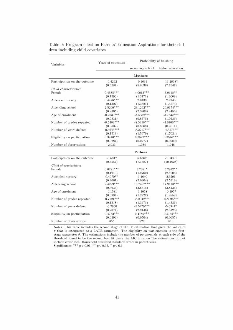
Table 9: Program effect on Parents’ Education Aspirations for their chil-dren including child covariates

VariablesYears of education

Probability of finishing

secondary school higher education

Mothers

Participation on the outcome -0.4262 -0.1631 -13.2668*(0.6287) (5.8036) (7.1347)

Child characteristicsFemale 0.4585*** 4.0013*** 3.9118**

(0.1290) (1.3171) (1.6008)Attended nursery 0.4476*** 2.0438 2.2148

(0.1307) (1.3321) (1.6573)Attending school 2.5200*** 23.1262*** 20.9174***

(0.2365) (2.3208) (2.4456)Age of enrolment -0.2633*** -3.5389*** -3.7532***

(0.0831) (0.8375) (1.0135)Number of grades repeated -0.5482*** -8.5456*** -4.6706***

(0.0802) (0.8868) (0.9611)Number of years defered -0.4643*** -8.2217*** -4.3576**

(0.1513) (1.5679) (1.7024)Eligibility on participation 0.3470*** 0.3522*** 0.3546***

(0.0284) (0.0277) (0.0280)Number of observations 2,033 1,984 1,948

Fathers

Participation on the outcome -0.5317 5.6562 -10.3391(0.6554) (7.1687) (10.1928)

Child characteristicsFemale 0.6221*** 3.7681* 5.2912**

(0.1940) (1.9760) (2.4206)Attended nursery 0.4970** -1.4640 2.3291

(0.2061) (2.0904) (2.5319)Attending school 2.4229*** 18.7497*** 17.9113***

(0.3936) (3.6315) (3.8134)Age of enrolment -0.1581 -1.4058 -0.4957

(0.0994) (1.2227) (1.2852)Number of grades repeated -0.7721*** -8.0049*** -6.8096***

(0.1318) (1.3471) (1.4331)Number of years defered -0.2900 -9.5479*** -5.0341*

(0.2074) (2.9146) (2.8128)Eligibility on participation 0.4732*** 0.4789*** 0.5132***

(0.0499) (0.0504) (0.0655)Number of observations 855 826 813

Notes: This table includes the second stage of the IV estimation that gives the values ofτ that is interpreted as a LATE estimator. The eligibility on participation is the first-stage parameter δ. The estimations include the number of polynomials at each side of thethreshold found to be the second best fit using the AIC criterion.The estimations do notinclude covariates. Household clustered standard errors in parentheses.Significance: *** p< 0.01, ** p< 0.05, * p< 0.1.

41

Table 10: Local linear regression of the poverty score counts at the cut-offfor eligibility

Time Preferences Education Expectations

All Urban Rural All Urban Rural

Eligibility -0.0667 0.7333 -0.8000 2.0333** 1.6333*** 0.4000(0.9491) (0.5465) (0.7061) (0.8961) (0.5505) (0.5777)

Constant 8.7667*** 3.2667*** 5.5000*** 6.9000*** 2.5333*** 4.3667***(0.6711) (0.3865) (0.4993) (0.6336) (0.3892) (0.4085)

Observations 60 60 60 60 60 60R-squared 0.0001 0.0301 0.0217 0.0815 0.1318 0.0082

Notes: We estimate an OLS model using the counts in bins of 0.05 from -1.5 to 1.5 in thepoverty score. Standard errors in parentheses.Significance: *** p< 0.01, ** p< 0.05, * p< 0.1.

42

Table 11: Discontinuities on the baseline covariates at thepoverty score cut-off for eligibility

All Rural Urban

Panel A: Households Composition

Number of children 6 to 17 0.5466*** 0.3080 0.4635(0.1821) (0.3298) (1.1153)

Number of children 0 to 6 -0.2793 -0.3117 -0.2552(0.2089) (0.2206) (0.5640)

Number of children 7 to 11 0.2261 0.2022 0.2232(0.3141) (0.3151) (0.4700)

Number of children 12 to 17 0.3616*** 0.2774 0.4789*(0.1271) (0.1863) (0.2647)

Number of females in the household 0.0789 0.2339 -0.0373(0.2292) (0.3606) (0.3715)

Number of people in the household 0.6219* 0.1371 0.5760(0.3230) (0.5655) (0.8916)

Number of caregivers 0.1325 0.1497 0.2521(0.0858) (0.2654) (0.2371)

Panel B: Households Head Characteristics

Age of the household head 1.9794 3.1518 1.8091(1.5627) (2.8880) (2.0944)

Years of education of the household head -1.0873** -0.5908 -0.5743(0.4777) (0.5703) (0.8868)

Notes: This table includes the second stage of the IV estimation that givesthe values of τ that is interpreted as a LATE estimator. The estimationsinclude the number of polynomials at each side of the threshold found to beof best fit using the AIC criterion.The estimations do not include covariates.Household clustered standard errors in parentheses.Significance: *** p< 0.01, ** p< 0.05, * p< 0.1.

43

Table 12: Effect of Program Participation on Time Preferences for current and past eligiblehouseholds

Current Participants Past Participants1

All Urban Rural All Urban Rural

Program effect -0.0215 -0.0573 0.0014 -0.0708 -0.0703 -0.0173(0.1400) (0.1430) (0.1540) (0.2506) (0.2955) (0.0839)

Discount rate for non-participants 0.7177*** 0.6731*** 0.7507*** 0.7712*** 0.7395*** 0.6963***(0.0937) (0.0827) (0.1119) (0.1066) (0.0840) (0.0327)

Eligibility on participation coefficient 0.4319*** 0.4679*** 0.4567*** 0.3370*** 0.3286** 0.6089***(0.0664) (0.0682) (0.0843) (0.1137) (0.1348) (0.0675)

Number of observations 1,993 1,035 958 788 376 412

Notes: This table includes the second stage of the IV estimation that gives the values of τ that is interpreted as aLATE estimator. The eligibility on participation is the first-stage parameter δ. The estimations include the numberof polynomials at each side of the threshold found to be of best fit using the AIC criterion.The estimations do notinclude covariates. Household clustered standard errors in parentheses.1 Participating in the past but no longer eligible because there are no longer children aged 0 to 17 in the household.Significance: *** p< 0.01, ** p< 0.05, * p< 0.1.

44

10 Figures

Figure 1: Histogram of the sample discount rate interval

45

Figure 2: Education level distribution at baseline by age cohort and region

46

Figure 3: Range of sample distribution on the poverty score by region

47

Figure 4: Probability of program participation by poverty score

48

Figure 5: Probability of program participation by poverty score and Urban/Rural region

49

Figure 6: Probability of program participation by poverty score for Parents in the aspira-tions sample

50

Figure 7: Effect of program participation on outcomes

51

Figure 8: Effect of program participation on outcomes for individuals in urban areas

52

Figure 9: Effect of program participation on outcomes for individuals in rural areas

53

Figure 10: Density of the poverty index in treatment municipalities by variable of interest

54

Figure 11: Density of the poverty index for Education Expectation sample by zone

55

11 References

Anderson, C. L., Dietz, M., Gordon, A., & Klawitter, M. (2004). Discount Rates in Vietnam. Economic Develop-ment & Cultural Change, 52 (4), 873-887.

Appadurai, A. (2004). The Capacity to Aspire: Culture and the Terms of Recognition. In V. Rao & M. Walton(Eds.), Culture and public action (pp. 59-84): Stanford: Stanford University Press, Stanford Social Sciences.

Attanasio, O., Battistin, E., Fitzsimons, E., & Vera-Hernandez, M. (2005). How effective are conditional cashtransfers? Evidence from Colombia IFS Briefing Notes BN54 London, UK: Institute for Fiscal Studies.

Attanasio, O., Battistin, E., & Mesnard, A. (2012). Food and Cash Transfers: Evidence from Colombia*. EconomicJournal, 122 (559), 92-124.

Attanasio, O., Fitzsimons, E., & Gomez, a. (2005). The impact of a conditional education subsidy on schoolenrolment in Colombia. Institute of Fiscal Studies.

Attanasio, O., Fitzsimons, E., Gomez, A., Gutierrez, M. I., Meghir, C., & Mesnard, A. (2010). Children’s Schoolingand Work in the Presence of a Conditional Cash Transfer Program in Rural Colombia. Economic Development andCultural Change, 58 (2), 181-210.

Attanasio, O., & Kaufmann, K. (2009). Educational Choices, Subjective Expectations, and Credit Constraints.National Bureau of Economic Research, Inc, NBER Working Papers: 15087.

Attanasio, O., & Kaufmann, K. (2014). Education choices and returns to schooling: Mothers’ and youths’ subjectiveexpectations and their role by gender. Journal of Development Economics, 109 (0), 203-216.

Attanasio, O., & Mesnard, A. (2006). The Impact of a Conditional Cash Transfer Programme on Consumption inColombia. Fiscal Studies, 27 (4), 421-442.

Baez, J. E., & Camacho, A. (2011). Assessing the long-term effects of conditional cash transfers on human capital:evidence from Colombia. The World Bank, Policy Research Working Paper Series: 5681.

Basu, K. (2003). Global labor standards and local freedoms: UNU World Institute for Development EconomicsResearch.

Bauer, M., & Chytilova, J. (2010). The Impact of Education on Subjective Discount Rate in Ugandan Villages.Economic Development & Cultural Change, 58 (4), 643-669.

Bauer, M., & Chytilova, J. (2013). Women, Children and Patience: Experimental Evidence from Indian Villages.Review of Development Economics, 17 (4), 662-675.

Becker, G. S., & Mulligan, C. B. (1997). The endogenous determination of time preference. Quarterly Journal ofEconomics, 112 (3), 729-758.

Benner, A. D., & Mistry, R. S. (2007). Congruence of mother and teacher educational expectations and low-incomeyouth’s academic competence. Journal of Educational Psychology, 99 (1), 140.

Bernard, T., Dercon, S., Orkin, K., & Taffesse, A. S. (2014). The future in mind: Aspirations and forward-lookingbehaviour in rural ethiopia. Paper presented at the Centre for the Study of African Economies conference oneconomic development in Africa, Oxford, UK, March.

Bowles, S. (1998). Endogenous preferences: The cultural consequences of markets and other economic institutions.Journal of economic literature, 75-111.

Bowles, S., Gintis, H., & Groves, M. O. (2009). Unequal chances: Family background and economic success:Princeton University Press.

Cameron, L., & Shah, M. (2015). Risk-taking behavior in the wake of natural disasters: Journal of Human

56

Resources, 50(2), 484-515.

Carvalho, L., Prina, S., & Sydnor, J. (2013). The Effects of Savings on Risk Attitudes and Intertemporal Choices.Unpublished manuscript.

Carvalho, L. S. (2010). Poverty and time preferences. RAND - Labour and Population, WR-759.

Chiapa, C., Garrido, J. L., & Prina, S. (2012). The effect of social programs and exposure to professionals on theeducational aspirations of the poor. Economics of Education Review, 31 (5), 778-798.

Cutler, D. M., & Lleras-Muney, A. (2010). Understanding differences in health behaviors by education. Journal ofHealth Economics, 29 (1), 1-28.

Das, J., Do, Q.-T., & Ozler, B. (2005). Reassessing conditional cash transfer programs. The World Bank ResearchObserver, 20 (1), 57-80.

Das, M. (2007). Persistent inequality: An explanation based on limited parental altruism. Journal of DevelopmentEconomics, 84 (1), 251-270.

Davis Kean, P. (2005). The Influence of Parent Education and Family Income on Child Achievement: The IndirectRole of Parental Expectations and the Home Environment. Journal of family psychology, 19 (2), 294-304.

De Janvry, A., & Sadoulet, E. (2005). Conditional cash transfer programs for child human capital development:Lessons derived from experience in Mexico and Brazil.

Dean, M., & Sautmann, A. (2014). Credit Constraints and the Measurement of Time Preferences. Available atSSRN 2423951.

Doepke, M., & Zilibotti, F. (2008). Occupational Choice and the spirit of capitalism. Quarterly Journal of Eco-nomics, 123 (2), 747-793.

Dohmen, T., Falk, A., Huffman, D., & Sunde, U. (2012). The Intergenerational Transmission of Risk and TrustAttitudes. The Review of Economic Studies, 79 (2), 645-677.

Duflo, E. (2006). Poor but rational. Understanding poverty, 367-378.

Edmonds, E. V. (2007). Child labor. Handbook of development economics, 4, 3607-3709.

Fernandez, R., & Fogli, A. (2009). Culture: An Empirical Investigation of Beliefs, Work, and Fertility. AmericanEconomic Journal: Macroeconomics, 1 (1), 146-177.

Fiszbein, A., Schady, N. R., & Ferreira, F. H. (2009). Conditional cash transfers: reducing present and futurepoverty: World Bank Publications.

Hahn, J., Todd, P., & Van der Klaauw, W. (2001). Identification and estimation of treatment effects with aregression-discontinuity design. Econometrica, 69 (1), 201-209.

Halle, T. G., Kurtz-Costes, B., & Mahoney, J. L. (1997). Family influences on school achievement in low-income,African American children. Journal of Educational Psychology, 89 (3), 527.

Imbens, G. W., & Angrist, J. D. (1994). Identification and estimation of local average treatment effects. Econo-metrica: Journal of the Econometric Society, 467-475.

Imbens, G. W., & Lemieux, T. (2008). Regression discontinuity designs: A guide to practice. Journal of Econo-metrics, 142 (2), 615-635.

Jensen, R. (2010). The (Perceived) Returns to Education and the Demand for Schooling. The Quarterly Journalof Economics, 125 (2), 515-548. doi: 10.1162/qjec.2010.125.2.515

Kirby, K. N., Godoy, R., Reyes-Garcia, V., Byron, E., Apaza, L., Leonard, W., . . . Wilkie, D. (2002). Correlates

57

of delay-discount rates: Evidence from Tsimane’ Amerindians of the Bolivian rain forest. Journal of EconomicPsychology, 23 (3), 291-316.

Kirk, C. M., Lewis-Moss, R. K., Nilsen, C., & Colvin, D. Q. (2011). The role of parent expectations on adolescenteducational aspirations. Educational Studies, 37 (1), 89-99.

Lawrance, E. C. (1991). Poverty and the rate of time preference: evidence from panel data. Journal of Politicaleconomy, 54-77.

Lee, D. S., & Lemieux, T. (2010). Regression Discontinuity Designs in Economics. Journal of economic literature,48 (2), 281-355.

Lemieux, T., & Lee, D. S. (2014). Regression Discontinuity. In H. Best & C. Wolf (Eds.), The SAGE Handbook ofRegression Analysis and Causal Inference: SAGE.

Martorano, B., Handa, S., Halpern, C., & Thirumurthy, H. (2014). Subjective Well-being, Risk Perceptions andTime Discounting: Evidence from a large-scale cash transfer programme: UNICEF Innocenti Research Centre.

McCrary, J. (2008). Manipulation of the running variable in the regression discontinuity design: A density test.Journal of Econometrics, 142 (2), 698-714.

Meier, S., & Sprenger, C. D. (2014). Temporal Stability of Time Preferences. Review of Economics and Statistics.

Mischel, W., Shoda, Y., & Rodriguez, M. L. (1989). Delay of gratification in children. Science, 244, 933+.

Pennings, J. M. E., & Garcia, P. (2005). The poverty challenge: How individual decision-making behavior influencespoverty. Economics Letters, 88 (1), 115-119.

Ray, D. (2006). Aspirations, poverty, and economic change. Understanding poverty, 409-421.

Rubalcava, L., Teruel, G., & Thomas, D. (2009). Investments, Time Preferences, and Public Transfers Paid toWomen. Economic Development & Cultural Change, 57 (3), 507-538.

Sosu, E. M. (2014). Predicting maternal aspirations for their children’s education: The role of parental and childcharacteristics. International Journal of Educational Research, 67, 67-79.

Spera, C., Wentzel, K., & Matto, H. (2009). Parental Aspirations for Their Children’s Educational Attainment:Relations to Ethnicity, Parental Education, Children’s Academic Performance, and Parental Perceptions of SchoolClimate. Journal of Youth and Adolescence, 38 (8), 1140-1152.

Tanaka, T., Camerer, C. F., & Nguyen, Q. (2006). Poverty, politics, and preferences: Field experiments and surveydata from Vietnam.

Volland, B. (2013). On the intergenerational transmission of preferences. Journal of Bioeconomics, 15 (3), 217-249.

Zilibotti, F., & Doepke, M. (2014). Parenting with Style: Altruism and Paternalism in Intergenerational PreferenceTransmission. Paper presented at the 2014 Meeting Papers.

Zumbuehl, M., Dohmen, T., & Pfann, G. (2013). Parental investment and the intergenerational transmission ofeconomic preferences and attitudes: SOEPpapers on Multidisciplinary Panel Data Research.

58