Can Behavioral Finance Explain the Term Structure Puzzles?

George Bulkley, Richard D. F. Harris and Vivekanand Nawosah

Xfi Centre for Finance and Investment University of Exeter

January 2007

Abstract We take advantage of the long series of short rate expectations that are implicit in the term structure to test two well-known behavioral models of biases in expectation formation. We find evidence consistent with these models. To investigate whether behavioral biases are sufficient to explain the scale of the empirical rejections of the expectations hypothesis we simulate behaviorally biased expectations of the short yield and use these to construct long yields. We apply the conventional tests to the simulated data and are able to generate rejections of the expectations hypothesis that are similar to those observed in practice. Keywords: Behavioral finance; Expectations hypothesis of the term structure of interest rates; Momentum; Return reversals. Address for correspondence: Professor Richard D. F. Harris, Xfi Centre for Finance and Investment, University of Exeter, Exeter EX4 4PU, UK. Tel: +44 (0) 1392 263215. Fax: +44 (0) 1392 263242. Email: R.D.F.Harris@exeter.ac.uk. We gratefully acknowledge financial support from the ESRC under research grant ACRR2784.

1. Introduction

The expectations hypothesis of the term structure of interest rates states that the yield on a

long bond is determined by the expectation of the short yield over the life of the long bond

plus a risk premium. The expectations hypothesis, in conjunction with the assumption of

rational expectations (henceforth we refer to these joint hypotheses as the REH) gives rise

to a number of testable implications for the movement of bond yields. The first is that the

expected future change in the spot yield that is implicit in the term structure of interest

rates is an unbiased forecast of the actual future change in the spot yield. The second is that

the spread between long and short bond yields, when suitably scaled, should be an

unbiased forecast of both next period’s change in the long bond yield and future changes in

the short yield over the life of the long bond. The third is that the actual yield spread should

be equal to the ‘theoretical’ yield spread that is based on the forecasts of future short yields

from a vector autoregression comprising the current short yield and the current yield spread.

These implications of the REH have been tested in a very large number of studies for

different countries, different time periods and different bond maturities. The collective

evidence from these tests suggests that the predictions of the REH are overwhelmingly

rejected.1

There has inevitably been a sustained effort to explain the empirical failure of the REH.

Perhaps the most obvious criticism of the REH is that it assumes that the risk premium is

constant. If the risk premium is in fact time-varying then empirical tests of the REH are

potentially biased. A number of studies have explored this possibility, and indeed tests that

allow for the possibility of a time-varying risk premium have generally produced weaker

rejections of the REH (see, for example, Fama, 1984; Evans and Lewis, 1994; Mankiw and

Miron, 1996). However, the results of these studies are sensitive to the choice of proxy for

the risk premium, the bond maturities considered and the sample period used.2 On balance,

it would appear that while the assumption of a constant risk premium might partially

explain the empirical failure of the REH, the scale of the rejection is simply too large to be

1 See, for example, Shiller (1979), Shiller et al. (1983), Campbell and Shiller (1984), Mankiw and Summers (1984), Mankiw (1986), Campbell and Shiller (1991) and Campbell (1995). Hardouvelis (1994) demonstrates that the rejection of the REH is not confined to the US. 2 See also Shiller et al. (1983), Jones and Roley (1983), Backus et al. (1987), Simon (1989), Froot (1989), Tzavalis and Wickens (1997) and Harris (2001).

2

fully accounted for by allowing the risk premium to be time-varying (see Backus et al.,

1994). Another explanation for the rejection of the REH is error in the measurement of the

long yield, which potentially induces a bias in standard tests of the REH (see, for example,

Stambaugh 1988). However, the reported rejections of the REH appear to be robust to such

measurement error. Campbell and Shiller (1991), for example, use instrumental variable

estimation to circumvent measurement error in the long yield and find that the REH is still

strongly rejected.

Bekaert et al. (1997) identify a further source of bias in tests of the REH that strengthens

the reported rejection of the REH. They assume that the short yield follows a stationary

first order autoregressive process and that agents use this model to forecast the short yield.

They show analytically that this leads to a small sample bias in tests of the REH that is

related to the downward bias of the OLS estimator of the autoregressive coefficient in the

short yield model, which is exacerbated by the fact that this coefficient is very close to

unity (see Kendall, 1954). Using Monte Carlo simulation, they show that the bias also

exists when the short yield and the yield spread are modeled simultaneously using a vector

autoregression. Even in the relatively large samples that are typically used in empirical

work, this bias remains significant. Bekaert et al. show that tests of the REH are biased in

such a way that the empirical evidence actually represents unambiguously stronger

evidence against the REH than asymptotic theory would imply.3

In this paper we investigate whether the failure of the REH might be due not to a failure of

the expectations hypothesis itself, but rather to a failure of the rational expectations

assumption. The possibility that agents might form systematically biased expectations has

received much attention in the equity market literature, where it has led to the development

of behavioral models that potentially explain various ‘anomalies’ in equity returns. These

behavioral models are based on well-established biases in perception and prediction that

are documented in experimental psychology. The key assumption of these models is that

agents systematically fail to update their expectations following new information in the

way that would be implied by Bayes’ rule. Empirically, behavioral models have been

shown to successfully explain the pervasive findings of short-term momentum and

long-term reversals in equity returns. In this paper, we examine whether these same 3 For further discussion of the statistical properties of tests of the REH, see also Bekaert and Hodrick (2001), Kool and Thornton (2004) and Thornton (2005).

3

behavioral models are able to explain the way in which expectations of the short rate are

formed in the bond market, and whether they can potentially account for the rejections of

the REH that have been reported in the literature.

One potential criticism of behavioral finance is that it is only able to explain the puzzles

that it was designed to explain, namely the observed anomalies in the equity market (see,

for example, Fama, 1998). We therefore study existing behavioral models that have been

developed in the equity market since the integrity of the behavioral approach is

undermined if new and different models must be designed to explain each new rejection of

rational expectations. If investors are subject to specific behavioral biases when they trade

in equity markets, it would be surprising if they did not exhibit the same biases when

trading in bond markets. If we find that the existing models that have been successful in the

equity market also explain biases in expectation formation in the bond market then this will

constitute ‘out of sample’ evidence in support of the behavioral approach, and thus counter

Fama’s critique that behavioral models must be tailored in an ad hoc fashion to rationalize

pre-existing anomalies.

The bond market represents an important test of behavioral models since data on agents’

expectations can be inferred directly from the term structure of interest rates. In contrast,

explicit data on agents’ expectations data are not available in equity markets, so support for

behavioral models can only be inferred from equity returns, for example by looking for

evidence of underreaction to public news events. The advantage of having an explicit series

of expectations, and the corresponding realisations, is that agents have an opportunity to

detect – and correct – any systematic patterns in expectational errors. In the equity market,

in contrast, such patterns must be filtered from returns data. Indeed, the attraction of

directly working with expectations data has led to the use of laboratory tests of specific

behavioral models (see, for example, Bloomfield and Hales, 2002). In these tests, subjects

are shown series of ‘realisations’ and are asked to form expectations about future values of

these series. The predictions of the behavioral model are then tested on the resulting data.

The bond market offers an opportunity to undertake a similar experiment, but with the

advantage over the laboratory setting that these are the expectations of experienced

participants with strong financial incentives to form unbiased expectations. If these

expectations are subject to behavioral biases then it is likely that these biases will be

pervasive.

4

Tests of the REH are greatly simplified by the use of zero coupon bond data. Since there

are only a limited number of traded zero coupon bonds in practice, one must rely on

synthetic data on zero coupon bond yields that are imputed from the yields of

coupon-paying bonds. Most of the studies cited above use the synthetic zero coupon bond

yield data of McCulloch and Kwon (1993). In this paper, we extend this data set to

December 2004 using data on coupon-paying bonds from the CRSP US Treasury Database.

In addition to testing the predictions of various behavioral finance models, we also provide

updated evidence on the REH itself. We find that consistent with earlier studies, the REH is

very strongly rejected for the extended sample, using all of the tests described above.

We take three approaches to evaluating behavioral models in the bond market. First, we

test whether the stylized facts of short-term momentum and long-term reversals in returns,

which are the hallmarks of behavioral models in the equity market, are present in the bond

market. Using monthly data on US zero coupon bonds over the period January 1952 to

December 2004, we find that there is significant positive serial correlation in short term

excess holding period returns in the bond market, and significant negative serial correlation

in long term excess holding period returns. The pattern of serial correlation in relation to

the length of the holding period is similar to that found in equity markets, although the

horizon over which momentum is found appears to be somewhat shorter.

Our second approach is to study the properties of the expectation errors that are implied by

two specific classes of behavioral models.4 The first builds on experimental evidence that

individuals over-extrapolate from short runs of data. This characteristic is sometimes

known as the ‘law of small numbers’ (LSN) and is a type of ‘representativeness’ bias (see,

for example, Kahneman and Tversky, 1971). The LSN describes the way in which

individuals expect the moments of a population to be reflected even in short samples of

data that are drawn from that population. Barberis et al. (1998) and Rabin (2002) show

how the LSN induces both short run momentum and long run reversals in returns. We show

below that this bias also induces positive short run serial correlation in the one-step ahead

4 There are other behavioural models that have been developed within the context of the equity market that do not have clear implications for bond returns. For example models where ‘winner’ stocks are sold and ‘loser’ stocks are held (see, for example, DeBondt and Thaler, 1985; DeBondt and Thaler, 1987).

5

forecast errors of the short yield, and negative serial correlation in average expectation

errors of the short yield at longer horizons. We test these predictions using the expectations

of short rates that are implicit in the term structure and find that both the short term and

long term implications of the ‘representativeness’ bias are confirmed. .

A second class of model builds on the widespread finding that individuals tend to be too

conservative when reacting to new information. In particular, agents attach too much

weight to their prior belief about the true model that generates the data, and too little

weight to recent information. The testable implications of this model are similar to those of

models that are based on the widespread observation that individuals are overconfident

about their ability. For example Daniel et al. (1998) show that overconfidence can lead to

underreaction to public news. In both cases, agents’ expectations following public news are

not immediately revised to the full extent that would be justified by (rational) Bayesian

updating. However, over time agents learn of their mistake, and so there are subsequent

revisions in agents’ expectations that are of the same sign as the initial response to the news

announcement. This model is supported by evidence of momentum in returns and is further

generally confirmed in the equity market with evidence from the event study literature.

Working with short rate expectations, we test and confirm the implication of the

conservatism and overconfidence biases, namely that revisions in expectations will be

positively serially correlated at short horizons, a prediction that is again clearly inconsistent

with rational expectations.

The empirical evidence summarized above is consistent with the predictions of behavioral

models. However are the behavioral biases sufficient to explain the observed rejections of

the REH in empirical work? Our third approach addresses this question. We undertake a

Monte Carlo experiment in which we simulate short yield data from a first order

autoregressive model (which is calibrated from the data), but generate expectations of the

short yield assuming that agents exhibit the ‘representativeness’ bias. We then use the

simulated short yield and the behaviorally biased forecasts of the short yield to construct

long yield data according to the expectations hypothesis (but not the rational expectations

hypothesis, since the expectations are not rational). Since there is no obvious way to

calibrate the expectations model, we specify the magnitude of the biases in the simulation

using a range of different parameter values. For each combination of parameter values, we

use the simulated data to test the REH using the standard tests described above. We find

6

that in most cases, the REH is very strongly rejected in the simulated data. Moreover, for

some plausible combinations of the model parameters, the pattern of rejection in the

simulated data (across different tests and different bond maturities) is very similar to the

pattern of rejection in the empirical tests. This suggests that the behavioral biases that have

been documented in the equity market are sufficient to explain the rejection of the REH in

the bond market.

The outline of this paper is as follows. In the following section, we describe the

construction of the new dataset of zero-coupon bond yields that we use in the empirical

sections of the paper. Section 3 presents the theory of the REH, and the empirical tests that

have been widely used to test the REH. We replicate these tests using the extended dataset.

In section 4, we describe the representativeness and conservatism biases, and derive the

testable implications of these biases for the bond market. The empirical results relating to

these biases are reported in Section 5. In Section 6, we undertake the simulation study and

repeat the empirical tests of the REH using the simulated data. Section 7 concludes.

2. Data

In this paper we use monthly zero-coupon bond yields on US Treasury securities for the

period January 1952 to December 2004.5 Most of the empirical studies of the REH

described in Section 3 make use of the McCulloch and Kwon (1993) monthly US term

structure data set (which is itself based on the McCulloch (1987) dataset).6 The McCulloch

and Kwon data comprise monthly time series of estimated zero-coupon yields, par bond

yields and instantaneous forward rates (and their respective standard errors) from

December 1946 to February 1991. The data are continuously compounded and are recorded

as annual percentages. Zero-coupon bond yields are available for 56 maturities from

overnight to 40 years.

For the purpose of this paper, we have updated the McCulloch and Kwon (1993) dataset to

December 2004. The data are constructed using the tax-adjusted cubic spline method of 5 Although data are available from December 1946, the quality of the estimated data improves significantly after the Treasury Accord of 1951 and so only data after this period are used, as recommended by McCulloch and Kwon (1993). 6The McCulloch and Kwon (1993) zero-coupon bond yield dataset can be found at www.econ.ohio-state.edu/jhm/ts/mcckwon/mccull.htm.

7

McCulloch (1975).7 The raw data were obtained from the CRSP US Treasury Database and

include all available quotations on US Treasury bills, notes and bonds.8 Since the raw data

that we use originate from a different source to McCulloch and Kwon, it is important to

check the integrity of the resulting estimated zero-coupon bond yields. We therefore

computed zero-coupon bond yields over a six-year overlapping period, August 1985 to

February 1991, and compared these with the corresponding yields reported in the

McCulloch and Kwon (1993) dataset.9 Panel A of Table 1 reports summary statistics for the

two datasets for the ten bond maturities that we use in this paper. For all ten bond

maturities, the correlation between the two datasets is in excess of 0.99, and for all except

the one month maturity, the correlation is in excess of 0.999.

[Table 1]

Figure 1 plots the estimated yields for the ten maturities over the overlapping period. For

maturities greater than one month, there is no discernable difference between the two

datasets. For the one-month maturity, there are some very minor discrepancies that arise

mainly from the use of a different raw data source. Panel B of Table 1 reports summary

statistics for the period covered by the McCulloch and Kwon data (January 1952 to

February 1991), for the extended period (March 1991 to December 2004), and for the

combined full sample. It is the full sample that we employ in the empirical sections of this

paper.

[Figure 1]

Figure 2 plots the estimated yields over the full sample. A striking feature of the extended

dataset is the evident structural break in each of the time series around 1980-82. Prior to 7 The authors are indebted to J. Huston McCulloch for kindly providing the FORTRAN program that fits the term structure of interest rates using the tax-adjusted cubic spline method and for his valuable help in resolving a number of problems associated with the construction of the data set. 8 Data on tax rates are obtained from the Internal Revenue Service, US Department of Treasury (www.irs.gov). 9 We choose the start date of August 1985 for the overlapping period on the grounds of convenience. Before this date, there are many more irregular bonds in the raw data which have to be manually deleted. Also, McCulloch and Kwon stopped using long-term callable bonds as from this date. For these reasons, it is easier to match the numbers in the original McCulloch and Kwon data set for August 1985-February 1991.

8

this, yields of all maturities secularly increased, while after this, they secularly decreased.

This has important implications for the empirical tests in the following sections. Under the

REH, rational expectations of this change in the long term trajectory of interest rates would

be impounded in long bond yields, and so there is no need to explicitly accommodate the

structural break under the null hypothesis that the REH holds. However, under the

alternative hypothesis that the REH does not hold, we cannot rule out the possibility,

suggested by visual inspection of the data, that there is a corresponding structural break in

agents’ expectation errors that is linked to the break between the long upward and

downward trends. It is important under the alternative hypothesis to accommodate this

structural break in tests of the REH. Structural breaks that are not explicitly modeled can

induce apparently systematic patterns in time series correlations (such as long memory)

that vanish once the structural break is explicitly introduced. In order to establish the

precise location of the structural break, we employ the structural stability test of Hansen

(1992). This indicates a breakpoint between June 1981 and June 1982, depending on the

regression estimated. For consistency, we assume a common breakpoint at December

1981.10 We explicitly allow for the structural break in all of the empirical tests by including

a dummy variable in each regression that is set to one for the period after the breakpoint

and zero otherwise.

[Figure 2]

3. The Expectations Hypothesis: Theory and Evidence

Consider an n-period zero coupon bond with unit face value, whose price at time t is .

The yield to maturity of the bond, , satisfies the relation

tnP ,

tnY ,

ntn

tn YP

)1(1

,, += (1)

10 We tested the robustness of the analysis to the location of the breakpoint. In general, we found that the empirical results are not sensitive to the exact choice of breakpoint. Indeed, for many of the regressions, excluding the dummy variable does not alter the qualitative conclusions that we draw.

9

or, in natural logarithms,

(2) tntn nyp ,, −=

where and )ln( ,, tntn Pp = )1ln( ,, tntn Yy += . If the bond is sold before maturity then the

log m-period holding period return, , where mmtnr +, nm < , is defined as the change in log

price, , which using (2) can be written as tnmtmn pp ,, −+−

(3) mtmntn

tnmtmnmtn

ymnnyppr

+−

+−+

−−=

−=

,,

,,,

)(

The expectations hypothesis states that the expected holding period return for bonds of

different maturities should be equal, except for a constant additive risk premium.

Combined with the rational expectations hypothesis, the expectations hypothesis of the

term structure has a number of important implications for the relationships between bond

yields, and their movement over time. In particular, the expectations hypothesis states that

the expected n-period return on an investment in a series of one-period bonds should be

equal to the (certain) n-period return on an n-period bond, which implies that the n-period

long yield should be an average of the expected short yield over the following n periods,

plus a constant risk premium.

n

n

iitttn yE

ny φ+= ∑

−

=+

1

0,1, )(1 (4)

where nφ is the risk premium and is the expectation conditional on the time t

information set. If expectations are rational then is the mathematical expectation.

We denote the relation given by (4) the expectations hypothesis (EH), even when

expectations are not rational. When expectations are rational, we denote the relation given

by (4) the rational expectations hypothesis (REH).

(.)tE

(.)tE

The earliest tests of the REH focus on the predictive ability of the expectations of future

spot yields that are implied by the term structure of interest rates. By combining expression

10

(4) for bonds of two different maturities, we can define m-period ‘forward’ yield for an

n-period bond as

nmmnyEnmyymnf

mtmnmtnt

tmtmnmtn

/))(()(/))((

,,

,,,

φφ −++=

−+=

++

+ (5)

The earliest tests of the REH directly examined whether the forward rates that are implied

by the term structure are unbiased predictors of future interest rates. This can be tested

using a regression of the form

mttnmtntnmtn yfyy ++ +−+=− ,1,,11,, )( εβα (6)

If forward rates are unbiased then the slope coefficient, 1β , should be equal to unity, while

the constant risk premium differential is captured by the intercept, 1α . This regression has

been estimated for values of m of between one month and twenty years, and for values of n

of between one month and five years. While forward rates clearly contain information that

is relevant for future spot rates, the estimated coefficient, 1β , is usually found to be

significantly less than unity (see, for example, Fama, 1984, and Fama and Bliss, 1987).

Here, we estimate this regression using the extended dataset, but include a dummy variable

that is set equal to one for the period after December 1981 and zero otherwise to capture

the structural break identified in Section 2.

mttnmtnttnmtn yfDyy ++ +−++=− ,1,,111,, )( εβγα (6a)

Table 2 reports the estimated parameters from this regression for two bond maturities and a

range of forward horizons. In particular, Panel A reports results for n = 1 month and m = 1,

3, 6, 9 and 12 months and, while Panel B reports results for n = 12 months and m = 12, 24,

36, 48, 60 and 120 months. Panel A therefore replicates the results of Fama (1984) over the

extended sample while Panel B replicates the results of Fama and Bliss (1987). Standard

errors are reported in parentheses.

[Table 2]

11

For the one-month yield, the estimated slope coefficient is significantly less than unity for

all horizons, at first declining with maturity and then rising with maturity. The coefficient

on the dummy variable is highly significant in all cases, highlighting the importance of the

structural break. For the 12-month yield, the estimated slope coefficient is significantly less

than unity for the 12-month and 24-month horizons, but significantly greater than unity for

longer horizons up to 60 months. For the 120-month horizon, the coefficient is greater than

unity, but not significantly so. Again the coefficient on the dummy variable is highly

significant in all cases. These results are very similar to those reported by Fama (1984) and

Fama and Bliss (1987) and strongly reject the REH.

A second way to test the predictions of the REH is to focus on the predictive ability of the

yield spread between long maturity and short maturity bonds, defined as . In

particular, rearranging equation (4) gives

ttntn yys ,1,, −=

nttnt

n

i

itt yyn

nyn

yEφ+−

−=−

−∑−

=

+ )(11 ,1,,1

1

1

,1 (7)

which states that the yield spread, when suitably scaled, should predict the cumulative

expected change in the short yield over the life of the long bond. Alternatively, combining

equation (4) for two adjacent bond maturities, and rearranging, gives.

nntntnttnt nnyy

nyyE φφ

1)(

11

111,1 −−+−

−=− −+− (8)

which states that the yield spread, when suitably scaled, should predict the following

period’s expected change in the yield on the long bond. These two predictions of the REH

can be tested with regressions of the form

1,21,22,1

1

1

,1 )(11 +

−

=

+ +−−

+=−−∑ tttnt

n

i

it yyn

nyny

εβα (9)

12

1,31,33,1,1 )(1

1++− +−

−+=− tttntntn yy

nyy εβα (10)

We call (9) the short yield regression and (10) the long yield regression. If the REH holds

then the coefficients 2β and 3β should be equal to unity, while the intercepts 2α and

3α capture the constant risk premium terms. Again, these tests have generated

overwhelming rejection of the REH. The coefficient 2β in equation (9) is typically found

to be significantly less than unity for short maturity bonds, but rising with maturity. For

long maturity bonds, it is often found to be significantly greater than unity. The coefficient

3β in equation (10) is typically found to be significantly less than unity, and falling with

maturity. For long maturity bonds, it is significantly less than zero (see, for example,

Campbell and Shiller, 1991; Bekaert et al., 1997; Bekaert and Hodrick, 2001).11 We

estimate these regressions, including a dummy variable that takes the value of unity for the

period after December 1981.

1,21,222,1

1

1

,1 )(11 +

−

=

+ +−−

++=−−∑ tttntt

n

i

it yyn

nDyny

εβγα (9a)

1,31,333,1,1 )(1

1++− +−

−++=− tttnttntn yy

nDyy εβγα (10a)

Table 3 reports the estimated parameters from regressions (9a) and (10a) estimated using

the extended dataset. For regression (9a), the standard errors are estimated using the

Newey and West (1987) estimator to allow for the fact that the dependent variable is

overlapping. The regressions are estimated for n = 3, 6, 9, 12, 24, 36, 48, 60 and 120

months. For the short-yield regression (9a), the estimated slope coefficient is significantly

lower than unity for short maturity bonds, and initially falls with maturity up to nine

months, but then rises with maturity. For the 120-month bond, the coefficient is

significantly greater than unity. For the long yield regression (10a), the estimated slope

11 Campbell and Shiller (1991) also test the REH using analogous regressions based on the yield spread between a variety of different bond maturities, tmtntn yys ,,, −= , for n between two months and 120 months and for m between one month and 60 months. The REH is strongly rejected for almost all pairs of bonds.

13

coefficient is negative and significantly lower than unity in all cases, and falls

monotonically with maturity. For all but the three-month bond, the coefficient is also

significantly less than zero.

These results for the extended sample are consistent with those reported by, for example,

Campbell and Shiller (1991) and Bekaert et al. (1997), for earlier periods. Like these

studies we find that the short rate regression rejects the REH decisively but evidence

against the REH from the long yield regression is much weaker. We also find that the

strength of rejections varies systematically with the horizon of the long bond in both

regressions in the same way as has been reported in earlier work. Why the strength of the

rejection should vary with the horizon of the long bond is an interesting and unexplained

feature of the empirical evidence.

[Table 3]

A third way to test the REH is the vector autoregression (VAR) approach of Campbell and

Shiller (1991). In particular, a pth-order VAR for the n-period spread, , and the change

in the short yield,

tns ,

ty ,1∆ , can be written in companion form as

ttntn AZZ ,41,, ε+= − (11)

where is a (2p x 1) vector comprising the current value and p – 1 lags of and the

current value and p – 1 lags of

tnZ , tns ,

ty ,1∆ , A is a (2p x 2p) matrix of parameters and t,4ε is a

(2p x 1) vector of errors. Forecasts of the n-period spread and the change in the short yield

are then given by . Using the expectations hypothesis relation (7), we can

then define the ‘theoretical’ spread as

tni

itn ZAZ ,,ˆ =+

tnn

tn ZAAIAInIAes ,11

, )1]())()(/1(['~ −− −−−−= (12)

where e is a (1 x 2p) ‘selection’ vector, such that tntn sZe ,,' = and I is the (2p x 2p)

identity matrix (see, for example, Campbell and Shiller, 1991). Since the conditioning

14

information in the VAR includes the current n-period spread, which itself embodies the

markets expectations of future short yields over the life of the long bond, the theoretical

spread should be equal to the actual spread. Campbell and Shiller (1991) suggested the

following two tests of the REH. Firstly, the correlation between the theoretical spread and

the actual spread should be equal to unity. Secondly, the ratio of the standard deviation of

the theoretical spread to the standard deviation of the actual spread should be equal to unity.

Using the McCulloch (1987) dataset, Campbell and Shiller (1991) find that while the

correlation coefficient is indeed close to unity, the ratio of the standard deviations is

typically around 0.5, thus strongly rejecting the REH.

Table 4 reports the correlation coefficient and standard deviation ratio for n = 3, 6, 12, 24,

36, 48, 60 and 120 months for the extended sample. The VAR was specified with a lag

length of four, chosen on the basis of the Schwartz Bayesian criterion, and includes a

dummy variable for the post-December 1981 period in each of the VAR equations. The

dummy variable is also incorporated into the expression for the theoretical spread given by

equation (12). The correlation coefficient rises with maturity, and for long maturity bonds,

it is not significantly different from one. For short maturity bonds, the correlation

coefficient is significantly less than one. The standard deviation ratio has a U-shaped

relationship with maturity, but is significantly lower than one for all bond maturities. These

results for the extended sample are consistent with the findings of Campbell and Shiller

(1991), again leading to a rejection of the REH.

[Table 4]

This section has replicated the existing empirical tests of the REH for the extended sample

of monthly US zero-coupon bond yields over the period January 1952 to December 2004.

Taken together, these tests represent overwhelming evidence against the REH. There are

two possible reasons for the failure of the REH to explain the movement of bond yields.

The first is that the expectations hypothesis of the term structure does not hold. However,

an alternative explanation is that the expectations hypothesis itself holds, but expectations

of future bond yields are not rational. We turn to this possibility in the following section.

15

4. Behavioral Models

Behavioral models are based on well-established biases in perception and prediction that

have been documented in experimental psychology. In this section, we describe some of

the documented behavioral biases on which these models are based, the ways in which

these biases have been used to explain anomalies in the equity market, and their testable

implications for the bond market.

4.1. Representativeness

Representativeness is the belief that a randomly drawn sample of data will display the

characteristics of the population from which it is drawn. Representativeness is related to

two specific behavioral biases that have been documented in the psychology literature. The

first is ‘base rate neglect’, which describes the finding that subjects put too little weight on

the unconditional probability of observing a particular sample. The second is ‘sample size

neglect’ or the ‘law of small numbers’, which describes the finding that subjects

overestimate the statistical relevance of information that is contained in the sample (see

Tversky and Kahneman, 1971). Both base rate neglect and sample size neglect cause

subjects to overweight (compared to a rational Bayesian) the importance of a given sample

of data when drawing inferences about the population from which it is drawn. Barberis et

al. (1998) and Rabin (2002) develop the implications of this bias for returns in equity

markets.

One consequence of this bias is sometimes described as the ‘gambler’s fallacy’ and this

formulation has testable implications for financial markets. The gambler’s fallacy describes

the finding that when subjects are asked to forecast drawings, with replacement, from an

urn with 50 percent red balls and 50 percent black balls, they tend to forecast a black ball

with a probability greater than 50 percent if a red ball was drawn previously. This bias

implies momentum in stock returns in the short run because if one period’s earnings

innovation is below that predicted by investors, investors give more than 50 percent weight

to the innovation next period being positive. However, under the correct model, the next

period’s innovation is positive with 50 percent probability, and hence investors will

experience a second negative surprise with more than 50 percent probability. This positive

serial correlation in earnings surprises translates into momentum in short horizon stock

16

returns. The market’s expectation of next period earnings is not directly observable, and so

this implication cannot be tested directly in the equity market. However, the serial

correlation in short run stock returns has been widely documented (see, for example, see

Jegadeesh and Titman, 1993; Jegadeesh and Titman, 2001) and is consistent with this

prediction for expectational errors.

The bond market offers an opportunity for a direct test of this hypothesis about expectation

formation since expectations about next period’s spot rate are implicit in the term structure

of interest rates. In particular, we are able to test whether there is positive short run serial

correlation in one-step ahead expectation errors for spot rates. This yields the first testable

hypothesis:

H1: mttmt yEy ++++ − 1,11,1 is positively serially correlated for small values of m

The preceding ‘gambler’s fallacy’ explains how subjects interpret sample data, given their

beliefs about the process that generated the sample. There are also interesting implications

for how subjects revise their beliefs about the data generating process. In particular,

subjects tend to employ ‘over-inference’, meaning that when they observe a series of

observations that don’t accord with their original beliefs about the true process (perhaps a

chance drawing of several red balls from the urn), they too readily interpret this as

evidence that their original beliefs were incorrect, and update their estimate of the true

process too quickly relative to a Bayesian. In the context of the above example, they too

quickly infer that the urn contains more than 50% red balls following a chance drawing of

several red balls.

Barberis et al. (1998) employ the representativeness heuristic to explain long-term return

reversals in the stock market. In particular, they posit that while earnings actually follow a

random walk, investors believe that earnings are either drawn from a ‘mean-reverting’

regime, or from a ‘trending’ regime. Investors believe that the dynamic process governing

earnings switches exogenously between these two regimes. By relying on recent earnings

performance, investors ‘identify’ the current regime and forecast next period’s earnings

accordingly. So, for example, if investors experience a series of positive earnings surprises

for a company (which results in a series of positive excess returns), they interpret this as

17

evidence that the company is a ‘high growth’ company, and consequently predict that

future earnings will also be high. In reality, however, this may just be an ‘average growth’

company that happened to have experienced a run of good earnings by chance. Therefore

investors will subsequently, on average, experience a negative earnings surprise (relative to

their expectations based on the revised model) leading to negative excess returns. Thus,

over the longer run, stock returns will be negatively serially correlated (see, for example,

DeBondt and Thaler, 1985; DeBondt and Thaler, 1987; Jegadeesh and Titman, 2001).

The implications of the representativeness bias in the bond market is that investors will

revise their model for the short rate after observing a series of positive shocks to the short

rate (relative to the model being used by investors to form expectations), and forecast

correspondingly higher values of the short rate into the future. In due course, it transpires

that these expectations are too high, which results in a series of negative shocks to the short

rate. This leads to the second testable hypothesis of the representativeness bias:

H2: ∑−

=++ −

−

1

1,1,1 )(

11 n

iittit yEy

n is negatively serially correlated at lag n for large values

of n

4.2. Conservatism

When confronted with the possibility that the true model is changing, the

representativeness bias implies that subjects are too quick to adopt a new model because,

relative to a Bayesian, they overweight the importance of the sample that they observe. In

contrast, ‘conservatism’ implies that subjects are too slow to revise their beliefs, because

they attach too much weight to their prior beliefs about the true model, and too little weight

to new information. In their regime-switching model, Barberis et al. (1998) combine

conservatism with representativeness. In particular, they assume that when earnings are in

the perceived ‘stationary’ regime and there is a large positive earnings ‘surprise’ (which is

actually just a chance drawing from a random walk), investors put too little weight on this

earnings observation, erroneously inferring that such an observation is just an outlier from

the stationary earnings regime. This is because they attach too much weight to their prior

belief that earnings are currently in a stationary regime. On the face of it, the conservatism

bias (which implies that agents underreact to new information) is at odds with the

18

representativeness (which assumes that agents overreact to new information). Barberis

(2003, page 1065) offers a way of reconciling the two biases: if an observed sample is

representative of a ‘salient’ model (i.e. one that concurs with the subject’s belief about the

set of probable models), then subjects will overweight the data. Conversely, if the observed

sample is not representative of a salient model, subjects will tend to underweight the data.

The existence of conservatism implies that investors should initially underreact to public

news about future interest rates, so that revisions in expectations of future spot rates will be

of the same sign in the periods following public news, as they are in the month in which

the news became public. For example, suppose that agents forecast the short rate using an

autoregressive model, and that public news is informative about future innovations in this

model. If investors underreact to news, revisions in expectations about the spot rate at

particular future dates will be positively serially correlated. Again data on revisions in

expectations can be inferred from the term structure and so this model can be tested

directly in the bond market. This leads to our third testable hypothesis:

H3: mttmtt yEyE +++ − ,1,11 is positively serially correlated for small values of m

5. Empirical Results

5.1. Evidence of Momentum and Return Reversals in the Bond Market

Before testing the hypotheses generated by the behavioral models described in the previous

section, we first investigate whether the stylized features of short-term momentum and

long-term return reversals that have been documented in the equity market, also exist in the

bond market. In particular, we estimate the degree of serial correlation in excess holding

period returns using the following regression.

mtmtmm

tnttmm

mtn myrDmyr +−+ +−++=− ,4,,444,, )( εβγα (13)

where the m-period holding period return for an n-period bond, , is defined by equation

(3). In all results in this section we include a dummy variable that takes the value of unity

for the period after December 1981 as explained above.

mtnr ,

19

Table 5 reports the results of estimating regression (13) for n = 2, 3, 6, 9, 12, 24, 36, 48, 60

and 120 months and m = 1, 2, 3, 6, 9, 12, 24, 36, 48 and 60 months. The regression is

estimated by OLS and standard errors are computed using the Newey and West (1987)

estimator to allow for the fact that the dependent variable is overlapping. Table 5 reveals

that the same patterns of short-run momentum and long-run return reversals that have been

documented in the equity market are also present in the bond market. In particular, for the

shortest holding period of one month, there is very significant positive serial correlation in

excess holding period returns for all bond maturities. The degree of serial correlation

decreases with bond maturity, but remains marginally significant even for long maturity

bonds. This suggests that there is short run momentum in excess holding period returns in

the bond market.12

For longer holding periods – between 24 and 120 months – there is very significant

negative serial correlation in excess holding period returns for longer maturity bonds,

suggesting that there are return reversals in excess holding period returns in the bond

market. This pattern of momentum and return reversals in the bond market is similar to that

found in the equity market, although the horizon over which there is significant momentum

in excess returns in the bond market is shorter than is typically found in the equity market

(see, for example, Jegadeesh and Titman, 1993).

[Table 5]

5.2. Tests of the Behavioral Hypotheses

We next test the specific predictions of the representativeness and conservatism models.

Table 6 reports the test of the short term implications of the representativeness bias,

hypothesis H1, which is that the one-step ahead expectation error of the short yield is

positively serially correlated. In order to test this hypothesis, we report the results of

estimating the following regression 12 Mankiw (1986) estimates the serial correlation in the excess holding period return for long term US Treasury bonds relative to the three month Treasury bill rate, using quarterly data over the period 1961-84, and finds that the first order autocorrelation coefficient is 0.02. The long bond yield used is an aggregate yield of bonds with maturities of 10 years or over. This is broadly consistent with the findings reported here.

20

tttttmtmtmt yEyDyEy ,5,11,1555,11,1 )( εβγα +−++=− −+−++ (14)

where is the forecast of that is implicit in the

current term structure of interest rates. The regression is estimated for lags m = 1, 2, 3, 4, 5

and 6 months.

tmtmmtt ymmyyE ,1,,1 )1( −+ −−= mty +,1

There is very significant positive serial correlation in one-step ahead expectation errors for

the short yield for horizons of one and two months. For longer horizons, there is no

significant serial correlation. This is consistent with the short run predictions of the LSN.

[Table 6]

Table 7 reports the test of the long term implications of the representativeness bias,

hypothesis H2, which is that the average (measured here over 6 or more months)

expectation error of the short yield is negatively serially correlated. Note that from (4)

n

n

iitttn yE

ny φ+= ∑

−

=+

1

0,1, )(1 , and so ntn

n

iit

n

iittit yy

nyEy

nφ−−=−

− ∑∑−

=+

−

=++ ,

1

0,1

1

1,1,1

1)(1

1 . We

therefore test H2 using the following regression

ttn

n

iittntn

n

iint yy

nDyy

n ,6,

1

0,1666,

1

0,1 )1(1 εβγα +−++=− ∑∑

−

=++

−

=++ (15)

The regression is estimated for horizons n = 6, 12, 18, 24, 36, 48, 60 and 120 months. The

estimated slope coefficient is significantly negative for horizons of 18 months and more,

rising at first and then falling. The strongest negative serial correlation is at a horizon of 48

months. This is consistent with the implication of the representativeness bias which implies

agents will revise their model too much in response to a short run of surprises resulting in

expectation errors that are negatively correlated.

[Table 7]

21

Table 8 reports the test of the conservatism bias, hypothesis H3, which is that expectation

revisions are positively serially correlated at short lags. In order to test this hypothesis, we

estimate the following regression

tmttmtttmttmtt yEyEDyEyE ,71,111,17771,11,11 )( εβγα +−++=− ++−+++++++ (16)

where . The regression is estimated for lags m = 1 to 12

months.

tmtmmtt ymmyyE ,1,,1 )1( −+ −−=

Consistent with hypothesis H3, there is positive serial correlation in the one-step ahead

expectation revisions for the short yield at all lags considered. The pattern of serial

correlation generally increases with autocorrelation lag up to about seven months, and then

declines monotonically. For all cases except 12 months, the positive serial correlation in

expectation revisions is statistically significant. Therefore, the prediction of the

conservatism bias – that one-step ahead expectation revisions in the short yield are

positively serially correlated – is strongly supported by the data.

[Table 8]

6. Monte Carlo Simulation

The empirical evidence reported in the previous section suggests that short rate

expectations are biased in a way that is consistent with two specific well-known behavioral

models. However are behavioral models sufficient to explain why the REH fails in

empirical tests? In order to address this issue, we undertake a Monte Carlo experiment. We

generate simulated short yield data from a model that is calibrated using the actual yield

data. We then simulate expectations of the short yield that are, by construction, subject to

the representativeness bias. Using the simulated data, we construct estimates of the long

yield according to the expectations hypothesis, and then test the REH using the tests

described in Section 3.

We first simulate data for the short yield using the following first-order autoregressive

(AR1) model.

22

ttt vyy ++= −1,1,1 985.0072.0 231.0)var( =tv (17)

The model was calibrated by estimating it over the full sample of monthly short yields

from January 1952 to December 2004. The lag length of one was chosen on the basis of the

Schwartz Bayesian Criterion. The estimated parameters were adjusted for the small sample

bias of Kendall (1954). We use (17) to generate 636 observations of the short yield (which

matches the empirical sample size used to test the REH in Section 3) with drawn from

a normal distribution. For simplicity, we do not include a structural break in the data

generating process, nor in the tests of the REH performed on the simulated data. Limited

experimentation suggested that the qualitative conclusion drawn from the simulation

experiments were independent of the inclusion of a structural break.

tv

In order to simulate behaviorally biased expectations of the short yield, we construct a

model of expectations based on the representativeness bias, incorporating both the

‘gambler’s fallacy’ element (which is relevant for short-run expectations) and the

‘over-inference’ element (which is relevant for long-run expectations). We assume that in

forecasting the short yield, agents start with the ‘true’ model given by (17). However, in

order to incorporate the short run and long run implications of the bias, we modify (17) in

two ways. Firstly, we assume that when agents forecast the following period’s short yield,

they predict that there will be a surprise that is opposite in sign to the current period’s

surprise, although to allow for varying degrees of bias, it is not necessarily equal in

magnitude. Secondly, we assume that when agents experience a series of surprises that are

non-zero on average, forecasts of the future short yield are adjusted as if the mean short

yield has changed by this average lagged surprise. We assume that the horizon considered

by investors is 12 months. Again, to allow for varying degrees of bias, the magnitude of the

revision is allowed to vary. This leads to the following model for simulating expectations

of the short yield.

tti

itt vcyvy ˆ985.0ˆ121072.0ˆ ,1

12

11,1 −++= ∑

=−+ θ (18)

23

where ⎟⎠

⎞⎜⎝

⎛++−= −

=−−∑ 1,1

12

11 985.0ˆ

121072.0ˆ t

iittt yvyv θ .

When 0=θ and , the forecasting model (18) reduces to the ‘true’ model given by

(17). Increasing

0=c

θ increases the importance of the short run component of the

representativeness bias, while increasing c increases the importance of the long run

component of the representativeness bias. To simulate data from this model, we must set

values of c and θ . Calibrating such a model is difficult, since we have no information

about the representativeness bias that would allow us to measure its quantitative

importance in such a model. We therefore instead report results for a range of values of c

and θ . In particular, we set c = 0.00, 0.10 and 0.20 and θ = 0.00, 0.10, 0.20 and 0.30.

Once we have simulated the actual short yield data, , and the behaviorally biased

expectations of the short yield, , we construct simulated long yield data, , using

the expectations hypothesis relation (4), for bond maturities n = 3, 6, 9, 12, 24, 36, 48, 60

and 120 months. We set the risk premium,

ty ,1

ty ,1ˆ tny ,

nφ , equal to zero for all maturities. We then test

the REH using (i) the forward yield regression given by (6), (ii) the yield spread

regressions given by (9) and (10) and (iii) the VAR tests based on the theoretical spread

given by (12). The simulation is performed using 1000 replications. In each case, we report

the average estimated coefficient and the standard deviation of the estimated coefficient

across the 1000 simulations. For reasons of brevity, we report only the estimated slope

parameter in each regression.

Table 9 reports the results of estimating the forward yield regression given by (6) for n = 1,

for the different values of c and θ . For c = 0.00 and θ = 0.00 (which corresponds to the

REH), the slope coefficient is significantly greater than one at all forward horizons. This

reflects the small sample bias of Bekaert, Hodrick and Marshall (1997), which arises from

the use of a highly persistent autoregressive process to generate the data. Holding c

constant, increasing θ leads to a reduction in the value of the slope coefficient, although

for c = 0.00, the coefficient remains greater than one in all cases. The impact on the slope

coefficient seems to be independent of the forward horizon. As c increases, however, the

coefficient rapidly declines, and for short horizons, the coefficient is lower than unity. For c

= 0.20 and θ = 0.20, the slope coefficient is significantly lower than unity for the one,

24

three and six month horizons, and marginally greater than unity for the nine and twelve

month horizons. Table 10 reports the results of estimating the forward yield regression

given by (6) for n = 12. In contrast with the case for n = 1, increasing c for a given value of

θ does not change the estimated slope coefficient very much, but increasing θ for a

given value of c leads to a reduction in the estimated slope coefficient, particularly shorter

horizons. For c = 0.20 and θ = 0.20, the estimated slope coefficient is marginally lower

than one for the 12 month horizon and marginally greater than one for longer horizons.

Comparing these simulation results with the corresponding results using the actual yield

data in Table 2, we can see that the simulated behavioral bias goes some way towards

explaining the rejection of the REH that we observe in practice using the forward yield

regression. In particular, it is able to generate estimated coefficients that are significantly

lower than unity for short horizons and significantly greater than unity for long horizons.

[Tables 9 and 10]

Table 11 reports the results of estimating the short yield regression given by (9) for the

different values of c and θ . For c = 0.00 and θ = 0.00, the slope coefficient is

significantly greater than one for all bond maturities, owing to small sample bias. The

average estimated values for this case are consistent with those reported by Bekaert,

Hodrick and Marshall (1997) in their simulation experiments. Increasing θ for a given

value of c leads to a reduction in the estimated slope coefficient, although it does not

appear to be monotonic. Increasing c leads to a further small reduction in the estimated

slope coefficient. For c = 0.20 and θ = 0.20, the estimated slope coefficient is marginally

lower than unity for short maturity bonds and marginally higher than unity for long

maturity bonds. Table 12 reports the results of estimating the long yield regression given

by (10). Here, increasing c has little impact on the estimated slope coefficient, while

increasing θ has a substantial impact. For c = 0.10 and c = 0.20, the slope coefficient is

not only less than unity, but also less than zero for almost all values of θ . The slope

coefficient declines with bond maturity for all combinations of c and θ .

Comparing these results with those reported in Table 3 using the actual yield data, we can

again see that the simulated behavioral bias captures many of the features of the empirical

rejections of the REH. In particular, for the short yield regression, for the higher values of c

25

andθ , the estimated slope coefficient is increasing in maturity, lower than one for short

maturity bonds and higher than one for long maturity bonds. For the long yield regression,

the slope coefficient is decreasing in maturity, lower than one for all bond maturities, and

lower than zero for all but the shortest maturity bonds.

[Tables 11 and 12]

Table 13 report the results of estimating the correlation coefficient between the actual

(simulated) yield spread and the theoretical (simulated) yield spread, given by equation

(12), for the different values of c and θ . Again, for c = 0.00 and θ = 0.00, the correlation

coefficient is significantly greater than one for all bond maturities owing to the small

sample bias of Bekaert, Hodrick and Marshall (1997). The correlation coefficient declines

as either c or θ increases, although for θ , the relationship is not monotonic. For c = 0.10

and c = 0.20, the correlation coefficient is significantly less than unity for short maturity

bonds, but close to unity for longer maturity bonds. Table 14 reports the results of

estimating the standard deviation ratio for the actual (simulated) yield spread and the

theoretical (simulated) yield spread, given by equation (12). Again, increasing either c or

θ reduces the standard deviation ratio, particularly for short maturity bonds. For c = 0.20

and θ = 0.30, the estimated standard deviation ratio is significantly lower than one for all

bond maturities.

Comparing these results for the simulated data with those reported in Table 4 once again

suggests that the two behavioral biases can potentially explain the rejection of the REH. In

particular, the correlation coefficient between the actual yield spread and the theoretical

yield spread is lower than unity for short maturity bonds, rising with maturity and

approximately equal to one for long maturity bonds. In contrast the standard deviation ratio

is significantly lower than unity for all bond maturities, rising slowly with bond maturity.

This pattern of results is replicated quite closely in the simulated data.

7. Conclusion

There is overwhelming evidence that the joint hypotheses of rational expectations and the

expectations model of the term structure do not both hold in the bond market. In this paper,

26

we explore the possibility that the failure of the REH is due not to a failure of the

expectations hypothesis itself, but rather to a failure of the assumption of rational

expectations that is implicit in empirical tests of the REH. To explore this issue, we draw

on the well-established literature on behavioral finance that has been developed to explain

the stylized features of short-term momentum and long-term return reversals in equity

returns. We focus on two particular classes of behavioral models – those based on

representativeness and conservatism – and derive the testable implications of these models

for expectations in the bond market. In contrast with the equity market – where investors’

expectations of earnings are not observable – expectations of the short yield can be inferred

from the term structure of interest rates, and so the bond market provides a valuable

opportunity to directly test the predictions of behavioral models. We find that the

predictions of these models are strongly supported by the data, suggesting that investors in

the bond market are indeed subject to these behavioral biases.

To investigate whether these biases might be sufficient to explain the reported rejections of

the REH we undertake a simulation experiment in which we generate expectations of the

short yield that are subject to the same two biases. Using the expectations hypothesis to

construct simulated long yields, we test the REH using data that, by construction, satisfies

the expectations hypothesis but is subject to the two behavioral biases. In most cases, the

REH is strongly rejected by standard tests using the simulated data. Furthermore specific

patterns of rejections across tests and bond maturities are very similar to those reported in

the empirical literature. We infer that the same behavioral biases that have been

documented in the equity market have the potential to explain the rejections of the REH in

the bond market. The evidence that the same biases are evident in both the bond and the

equity market, and can moreover explain a pre-existing puzzle in the bond market,

provides further support for behavioral finance.

27

References Backus, D.K., Gregory, A. and Zin, S.E., 1994, Risk Premiums in the Term Structure: Evidence from Artificial Economies" Journal of Monetary Economics 24 371-399. Barberis, N., A. Shliefer, and R. Vishny, 1998, “A Model of Investor Sentiment”, Journal of Financial Economics 49, pp. 307-343. Bekaert, G., and R. Hodrick, 2001, “Expectations Hypothesis Tests”, Journal of Finance 56, 1357-1394. Bekaert, G., R. Hodrick and D. Marshall, 1997, “On Biases in Tests of the Expectations Hypothesis of the Term Structure of Interest Rates,” Journal of Financial Economics 44, 309-348. Bloomfield, R. J. and J. Hales, 2002, “Predicting the Next Step of a Random Walk: Experimental Evidence of Regime-Shifting Beliefs,” Journal of Financial Economics 65, 397-414. Campbell, J., 1995, “Some Lessons from the Yield Curve,” Journal of Economic Perspectives 9, 125-152. Campbell, J., and R. Shiller, 1984, “A Simple Account of the Behavior of Long Term Interest Rates,” American Economic Review, Papers and Proceedings 74, 44-48. Campbell, J., and R. Shiller, 1991, “Yield Spreads and Interest Rate Movements: A Bird's Eye View,” Review of Economic Studies 58, 495-514. Daniel, K., D. Hirshleifer and A. Subrahmanyam, 1998, “Investor Psychology and Security Under- and Overreactions,” Journal of Finance 53, 1839-1885. DeBondt, W. F. M., and R. H. Thaler, 1985, “Does the Stock Market Overreact,” Journal of Finance 40, 557-581. DeBondt, W. F. M., and R. H. Thaler, 1987, “Further Evidence on Investor Overreaction and Stock Market Seasonality,” Journal of Finance 42, 3, 557-581 Evans, M., and K. Lewis, 1994, “Do Stationary Risk Premia Explain It All? Evidence from the Term Structure” Journal of Monetary Economics 33, 285-318. Fama, E., 1984, “The Information in the Term Structure” Journal of Financial Economics 13, 509-528. Fama, E. F., 1998, “Market Efficiency, Long Term Returns, and Behavioral Finance,” Journal of Financial Economics 49, 283-306. Fama, E. F. and R. R. Bliss, 1987, "The Information in Long-Maturity Forward Rates," American Economic Review 77, 4, 680-692. Froot, K., 1989, “New Hope for the Expectations Hypothesis of the Term Structure of

28

Interest Rates,” Journal of Finance 44, 283-305. Hardouvelis, G., 1994, “The Term Structure Spread and Future Changes in Long and Short Rates in the G7 Countries: Is There a Puzzle?” Journal of Monetary Economics 33, 255-283. Harris, R. D. F. (2001), “The Expectations Hypothesis of the Term Structure and Time Varying Risk Premia: A Panel Data Approach”, Oxford Bulletin of Economics and Statistics 63, 233-245. Jones, D., and V. Roley, 1983, “Rational Expectations and the Expectations Model of the Term Structure: A Test Using Weekly Data,” Journal of Monetary Economics 12, 453-465. Kendall, M., (1954), “Note on the Bias in the Estimation of Autocorrelation,” Biometrika 41, 403-404. Kool, C., and D. Thornton, (2004) “A Note on the Expectations Theory and the Founding of the FED”, Journal of Banking and Finance 28, 3055-68 Mankiw, N., 1986, “The Term Structure of Interest Rates Revisited,” Brookings Papers on Economic Activity 1, 61-96. Mankiw, N., and J. Miron, 1986, “The Changing Behavior of the Term Structure of Interest Rates,” Quarterly Journal of Economics 101, 211-228. Mankiw, N., and L. Summers, 1984, “Do Long Term Interest Rates Overreact to Short Term Interest Rates?” Brookings Papers on Economic Activity 1, 223-242. McCulloch, H., and H. Kwon, 1993, “U. S. Term Structure Data, 1947-1991,” Working Paper 93-6, Ohio State University. Newey W. K. and K. D. West, 1987, “A Simple, Positive Definite, Heteroskedasticity and Autocorrelation Consistent Covariance Matrix.” Econometrica 55, 3, 703-708. Rabin, M., 2002, “Inference by Believers in the Law of Small Numbers,” Quarterly Journal of Economics 117, 775-816. Shiller, R., 1979, “The Volatility of Long Term Interest Rates and Expectations Models of the Term Structure,” Journal of Political Economy 82, 1190-1219. Shiller, R., J. Campbell and K. Schoenholtz, 1983, “Forward Rates and Future Policy: Interpreting the Term Structure of Interest Rates,” Brookings Papers on Economic Activity 1, 173-217. Simon, D., 1989, “Expectations and Risk in the Treasury Bill Market: An Instrumental Variables Approach,” Journal of Financial and Quantitative Analysis 24, 357-368. Stambaugh, R., 1988, “The Information in Forward Rates: Implications for Models of the Term Structure,” Journal of Financial Economics 21, 41-70.

29

Thornton, D., 2005, “Tests of the Expectations Hypothesis: Resolving the Campbell-Shiller Paradox,” Journal of Money, Credit and Banking, forthcoming. Tvseky, A., and D. Kahnman, 1971, “Belief in the Law of Small Numbers,” Psychological Bulletin 76, 105-110. Tzavalis, E., and M. Wickens, 1997, “Explaining the Failure of the Term Spread Models of the Rational Expectations Hypothesis of the Term Structure,” Journal of Money, Credit and Banking 29, 364-380.

30

Figure 1 McCulloch-Kwon and New Zero-Coupon Bond Yields for 08/1985-02/1991

—— McCulloch-Kwon data – – – New Data

1 month

Date

% p

er a

nnum

1985 1986 1987 1988 1989 19900.0

2.5

5.0

7.5

10.0 2 year

Date

% p

er a

nnum

1985 1986 1987 1988 1989 19900.0

2.5

5.0

7.5

10.0

3 month

Date

% p

er a

nnum

1985 1986 1987 1988 1989 19900.0

2.5

5.0

7.5

10.0

3 year

Date

% p

er a

nnum

1985 1986 1987 1988 1989 19900

2

4

6

8

10

6 month

Date

% p

er a

nnum

1985 1986 1987 1988 1989 19900.0

2.5

5.0

7.5

10.0 4 year

Date

% p

er a

nnum

1985 1986 1987 1988 1989 19900.0

2.5

5.0

7.5

10.0

9 month

Date

% p

er a

nnum

1985 1986 1987 1988 1989 19900.0

2.5

5.0

7.5

10.0 5 year

Date

% p

er a

nnum

1985 1986 1987 1988 1989 19900

2

4

6

8

10

1 year

Date

% p

er a

nn

um

1985 1986 1987 1988 1989 19900.0

2.5

5.0

7.5

10.0 10 year

Date

% p

er a

nnum

1985 1986 1987 1988 1989 19900.0

1.6

3.2

4.8

6.4

8.0

9.6

11.2

Notes: The figure plots the McCulloch and Kwon (1993) and new zero-coupon bond yields over the overlapping period 08/1985-02/1991 for the ten bond maturities that are used in the paper.

31

Figure 2 Zero-Coupon Bond Yields for the Full Sample 01/1952-12/2004

1 month

Date

% p

er a

nnum

1952 1956 1960 1964 1968 1972 1976 1980 1984 1988 1992 1996 2000 20040.0

2.5

5.0

7.5

10.0

12.5

15.0

17.52 year

Date

% p

er a

nnum

1952 1956 1960 1964 1968 1972 1976 1980 1984 1988 1992 1996 2000 20040.0

2.5

5.0

7.5

10.0

12.5

15.0

17.5

3 month

Date

% p

er a

nn

um

1952 1956 1960 1964 1968 1972 1976 1980 1984 1988 1992 1996 2000 20040.0

2.5

5.0

7.5

10.0

12.5

15.0

17.53 year

Date

% p

er a

nn

um

1952 1956 1960 1964 1968 1972 1976 1980 1984 1988 1992 1996 2000 20040

2

4

6

8

10

12

14

16

6 month

Date

% p

er a

nnum

1952 1956 1960 1964 1968 1972 1976 1980 1984 1988 1992 1996 2000 20040.0

2.5

5.0

7.5

10.0

12.5

15.0

17.54 year

Date

% p

er a

nnum

1952 1956 1960 1964 1968 1972 1976 1980 1984 1988 1992 1996 2000 20040

2

4

6

8

10

12

14

16

9 month

Date

% p

er a

nn

um

1952 1956 1960 1964 1968 1972 1976 1980 1984 1988 1992 1996 2000 20040.0

2.5

5.0

7.5

10.0

12.5

15.0

17.55 year

Date

% p

er a

nn

um

1952 1956 1960 1964 1968 1972 1976 1980 1984 1988 1992 1996 2000 20040

2

4

6

8

10

12

14

16

1 year

Date

% p

er a

nnum

1952 1956 1960 1964 1968 1972 1976 1980 1984 1988 1992 1996 2000 20040.0

2.5

5.0

7.5

10.0

12.5

15.0

17.510 year

Date

% p

er a

nnum

1952 1956 1960 1964 1968 1972 1976 1980 1984 1988 1992 1996 2000 20040

2

4

6

8

10

12

14

16

Notes: The figure plots the zero-coupon bond yields for the full sample 01/1952-12/2004 for the ten bond maturities that are used in the paper.

32

Table 1 Summary Statistics

Panel A

n McCulloch-Kwon data (Aug. 1985 - Feb. 1991) New data (Aug. 1985 - Feb. 1991) (months)

Mean Std Error

Minimum

Maximum

Mean Std Error

Minimum

Maximum

Correlation

1 6.528 1.193 3.800 9.043 6.527 1.176 3.948 9.248 0.99125 3

6.936 1.057 5.242 9.053 6.935 1.058 5.243 9.056 0.99963 6 7.104 0.977 5.262 9.279 7.102 0.976 5.261 9.314 0.99975

12 7.388 0.927 5.485 9.490 7.390 0.931 5.488 9.545 0.99953 24 7.726 0.821 5.988 9.454 7.734 0.824 6.003 9.527 0.99938 36 7.918 0.775 6.247 9.417 7.915 0.780 6.218 9.470 0.99923 48 8.046 0.748 6.505 9.559 8.044 0.747 6.535 9.572 0.99967 60 8.149 0.743 6.648 9.859 8.155 0.738 6.775 9.899 0.99930

120 8.486 0.715 7.274 10.459 8.479 0.716 7.271 10.459 0.99957

Panel B

n McCulloch-Kwon data (Jan. 1952 - Feb. 1991) New data (Mar. 1991 - Dec. 2004) Extended data (Jan. 1952 - Dec. 2004) (months)

Mean Std Error

Minimum

Maximum

Mean Std Error

Minimum

Maximum

Mean Std Error Minimum Maximum

1 5.314 3.064 0.249 16.210 3.716 1.584 0.773 6.210 4.896 2.842 0.249 16.2103

5.640 3.143 0.615 15.999 3.908 1.650 0.865 6.291 5.188 2.929 0.615 15.9996 5.884 3.178 0.685 16.511 4.033 1.668 0.955 6.456 5.401 2.974 0.685 16.511

12 6.079 3.168 0.847 16.345 4.275 1.686 1.034 7.142 5.608 2.963 0.847 16.34524 6.272 3.124 1.149 16.145 4.672 1.610 1.271 7.569 5.854 2.894 1.149 16.14536 6.386 3.087 1.412 15.825 4.968 1.487 1.616 7.684 6.016 2.829 1.412 15.82548 6.467 3.069 1.595 15.847 5.221 1.396 2.017 7.712 6.142 2.786 1.595 15.84760 6.531 3.056 1.770 15.696 5.387 1.323 2.359 7.911 6.232 2.758 1.770 15.696

120 6.683 3.013 2.341 15.065 5.957 1.118 3.608 8.325 6.493 2.670 2.341 15.065 Notes: The table reports summary statistics for the McCulloch and Kwon (1993) and new zero-coupon bond yield datasets for the ten bond maturities that are used in the paper. Panel A reports summary statistics for the overlapping period 08/1985-02/1991. Panel B reports summary statistics for the two sub-samples 01/1952-02/1991 and 03/1991-12/2004, and for the full sample.

33

Table 2 Forward Yield Regressions

Panel A: Forecasts of 1-month spot rates (n = 1)

Panel B: Forecasts of 1-year spot rates (n = 12)

m 1α 1γ 1β m 1α 1γ 1β

1 -0.155 -0.054 0.504 12 0.253 -1.068 0.413 (0.034) (0.043) (0.053) (0.087) (0.143) (0.105)

3 -0.198 -0.163 0.434 24 0.310 -2.173 0.827 (0.068) (0.078) (0.069) (0.115) (0.190) (0.098)

6 -0.122 -0.399 0.353 36 0.335 -3.547 1.353 (0.091) (0.103) (0.073) (0.113) (0.186) (0.084)

9 -0.108 -0.718 0.444 48 0.378 -4.281 1.558 (0.096) (0.119) (0.074) (0.110) (0.180) (0.075)

12 -0.178 -1.077 0.582 60 0.479 -4.860 1.494 (0.105) (0.141) (0.074) (0.117) (0.201) (0.077) 120 1.360 -6.939 1.094 (0.146) (0.294) (0.093)

Notes: The table reports the results of estimating the forward yield regression (6a) in the main text for the full sample 01/1952-12/2004, including a dummy variable that is set equal to one for the period after December 1981 and zero otherwise. Panel A reports results for forecasts of the 1-month yield at forward horizons of 3, 6, 9 and 12 months. Panel B reports results for forecasts of the 12-month yield at forward horizons of 12, 24, 36, 48, 60 and 120 months. Standard errors are reported in parentheses.

34

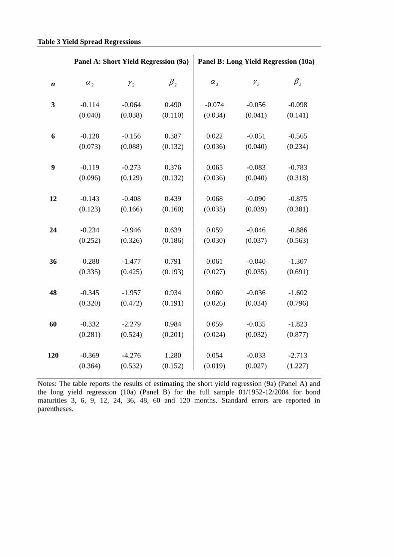
Table 3 Yield Spread Regressions

Panel A: Short Yield Regression (9a) Panel B: Long Yield Regression (10a)

n 2α 2γ 2β 3α 3γ 3β

3 -0.114 -0.064 0.490 -0.074 -0.056 -0.098 (0.040) (0.038) (0.110) (0.034) (0.041) (0.141)

6 -0.128 -0.156 0.387 0.022 -0.051 -0.565 (0.073) (0.088) (0.132) (0.036) (0.040) (0.234)

9 -0.119 -0.273 0.376 0.065 -0.083 -0.783 (0.096) (0.129) (0.132) (0.036) (0.040) (0.318)

12 -0.143 -0.408 0.439 0.068 -0.090 -0.875 (0.123) (0.166) (0.160) (0.035) (0.039) (0.381)

24 -0.234 -0.946 0.639 0.059 -0.046 -0.886 (0.252) (0.326) (0.186) (0.030) (0.037) (0.563)

36 -0.288 -1.477 0.791 0.061 -0.040 -1.307 (0.335) (0.425) (0.193) (0.027) (0.035) (0.691)

48 -0.345 -1.957 0.934 0.060 -0.036 -1.602 (0.320) (0.472) (0.191) (0.026) (0.034) (0.796)

60 -0.332 -2.279 0.984 0.059 -0.035 -1.823 (0.281) (0.524) (0.201) (0.024) (0.032) (0.877)

120 -0.369 -4.276 1.280 0.054 -0.033 -2.713 (0.364) (0.532) (0.152) (0.019) (0.027) (1.227)

Notes: The table reports the results of estimating the short yield regression (9a) (Panel A) and the long yield regression (10a) (Panel B) for the full sample 01/1952-12/2004 for bond maturities 3, 6, 9, 12, 24, 36, 48, 60 and 120 months. Standard errors are reported in parentheses.

Table 4 VAR Correlation and Standard Deviation Ratio

n Correlation SD ratio

3 0.872 0.564

6 0.799 0.493

9 0.820 0.454

12 0.867 0.462

24 0.945 0.499

36 0.973 0.543

48 0.983 0.576

60 0.988 0.600

120 0.996 0.708

Notes: The table reports the correlation coefficient and standard deviation ratio between the actual yield spread and the theoretical yield spread given by equation (12), for bond maturities 3, 6, 9, 12, 24, 36, 48, 60 and 120 months. Standard errors are reported in parentheses

36

Table 5 Momentum and Return Reversals

m n 1 2 3 6 9

2 4α 0.243 (0.032) 4γ 0.041 (0.045) 4β 0.266 (0.038)

3 4α 0.379 (0.059) 0.395 (0.072) 4γ 0.099 (0.085) 0.104 (0.075) 4β 0.182 (0.039) 0.148 (0.078)

6 4α 0.559 (0.137) 0.953 (0.284) 1.105 (0.315) 4γ 0.194 (0.204) 0.310 (0.294) 0.321 (0.334) 4β 0.186 (0.039) 0.063 (0.092) 0.022 (0.118)

9 4α 0.451 (0.217) 0.819 (0.467) 1.085 (0.561) 1.113 (0.438) 4γ 0.640 (0.328) 1.279 (0.491) 1.668 (0.632) 1.614 (0.616) 4β 0.168 (0.039) -0.001 (0.108) -0.067 (0.123) -0.055 (0.113)

12 4α 0.351 (0.286) 0.556 (0.608) 0.638 (0.768) 0.573 (0.844) 0.673 (0.575) 4γ 1.118 (0.436) 2.439 (0.690) 3.508 (0.953) 4.754 (1.277) 2.716 (0.850) 4β 0.175 (0.039) 0.004 (0.107) -0.059 (0.123) -0.054 (0.101) 0.114 (0.073)

24 4α 0.020 (0.540) -0.263 (1.049) -0.146 (1.429) -1.133 (2.132) -1.508 (2.511) 4γ 1.768 (0.821) 4.185 (1.381) 7.336 (2.016) 13.085 (3.495) 15.092 (4.180) 4β 0.140 (0.039) -0.050 (0.095) -0.084 (0.110) -0.045 (0.085) 0.071 (0.072)

36 4α -0.253 (0.761) -0.937 (1.389) -1.763 (1.844) -2.946 (3.084) -5.826 (3.709) 4γ 2.744 (1.159) 6.395 (2.007) 9.958 (2.894) 20.917 (5.370) 23.368 (6.445) 4β 0.109 (0.040) -0.054 (0.085) -0.106 (0.096) -0.035 (0.079) -0.023 (0.071)

48 4α -0.558 (0.960) -1.657 (1.693) -2.853 (2.255) -6.120 (3.691) -8.845 (4.961) 4γ 3.677 (1.463) 8.526 (2.574) 13.114 (3.715) 23.875 (6.658) 32.462 (8.597) 4β 0.095 (0.040) -0.063 (0.078) -0.098 (0.089) -0.049 (0.077) -0.034 (0.077)

60 4α -0.869 (1.136) -2.376 (1.941) -3.915 (2.592) -8.101 (4.358) -11.884 (6.000) 4γ 4.537 (1.731) 10.438 (3.071) 15.868 (4.443) 29.079 (8.010) 40.626 (10.487) 4β 0.086 (0.040) -0.064 (0.073) -0.086 (0.085) -0.036 (0.076) -0.034 (0.081)

120 4α -2.432 (1.881) -5.963 (2.917) -9.348 (3.935) -18.205 (7.024) -27.775 1(0.227) 4γ 8.317 (2.866) 18.815 (5.192) 28.404 (7.574) 52.357 1(3.792) 78.007 1(8.737) 4β 0.068 (0.040) -0.056 (0.065) -0.064 (0.077) -0.010 (0.076) -0.051 (0.090)

Notes: The table reports the results of estimating regression (13) for the full sample 01/1952-12/2004 for bond maturities 3, 6, 9, 12, 24, 36, 48, 60 and 120 months, and holding periods 1, 2, 3, 6, 9, 12, 24, 36, 48 and 60 months.

37

Table 5 Momentum and Return Reversals (Continued)

m n 12 24 36 48 60

2 4α 4γ 4β

3 4α 4γ 4β

6 4α 4γ 4β

9 4α 4γ 4β

12 4α 4γ 4β

24 4α -1.474 (2.795) 4γ 16.975 (4.497) 4β 0.006 (0.107)

36 4α -4.809 (4.909) -5.089 (4.928) 4γ 31.837 (7.942) 35.770 (6.969) 4β -0.046 (0.110) -0.257 (0.135)

48 4α -8.746 (6.656) -12.829 (8.661) -9.112 (6.042) 4γ 46.387 1(0.759) 65.989 1(2.746) 53.720 (8.790) 4β -0.091 (0.112) -0.271 (0.122) -0.456 (0.068)

60 4α -13.167 (8.199) -21.685 (11.717) -21.942 (11.240) -12.637 (6.627) 4γ 58.504 (13.223) 92.872 (17.666) 97.559 (16.073) 64.405 (9.424) 4β -0.124 (0.117) -0.288 (0.110) -0.434 (0.066) -0.505 (0.105)

120 4α -38.521 (14.162) -73.040 (24.566) -99.777 (33.003) -113.646 (33.179) -106.109 (30.256) 4γ 118.637 (22.499) 210.297 (38.753) 279.988 (44.332) 319.132 (39.181) 306.259 (38.683) 4β -0.200 (0.129) -0.307 (0.101) -0.387 (0.080) -0.471 (0.077) -0.464 (0.114) Notes: The table reports the results of estimating regression (13) for the full sample 01/1952-12/2004 for bond maturities 3, 6, 9, 12, 24, 36, 48, 60 and 120 months, and holding periods 1, 2, 3, 6, 9, 12, 24, 36, 48 and 60 months.

38

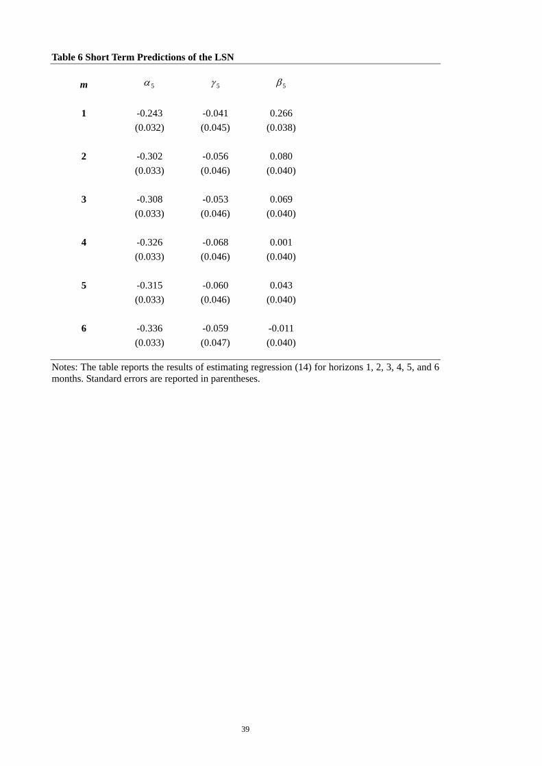
Table 6 Short Term Predictions of the LSN

m 5α 5γ 5β

1 -0.243 -0.041 0.266 (0.032) (0.045) (0.038)

2 -0.302 -0.056 0.080 (0.033) (0.046) (0.040)

3 -0.308 -0.053 0.069 (0.033) (0.046) (0.040)

4 -0.326 -0.068 0.001 (0.033) (0.046) (0.040)

5 -0.315 -0.060 0.043 (0.033) (0.046) (0.040)

6 -0.336 -0.059 -0.011 (0.033) (0.047) (0.040)

Notes: The table reports the results of estimating regression (14) for horizons 1, 2, 3, 4, 5, and 6 months. Standard errors are reported in parentheses.

39

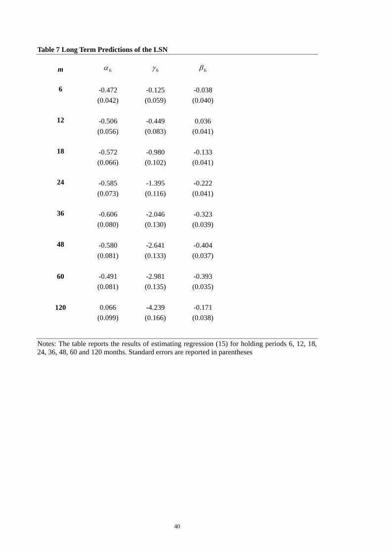
Table 7 Long Term Predictions of the LSN

m 6α 6γ 6β

6 -0.472 -0.125 -0.038 (0.042) (0.059) (0.040)

12 -0.506 -0.449 0.036 (0.056) (0.083) (0.041)

18 -0.572 -0.980 -0.133 (0.066) (0.102) (0.041)

24 -0.585 -1.395 -0.222 (0.073) (0.116) (0.041)

36 -0.606 -2.046 -0.323 (0.080) (0.130) (0.039)

48 -0.580 -2.641 -0.404 (0.081) (0.133) (0.037)

60 -0.491 -2.981 -0.393 (0.081) (0.135) (0.035)

120 0.066 -4.239 -0.171 (0.099) (0.166) (0.038)

Notes: The table reports the results of estimating regression (15) for holding periods 6, 12, 18, 24, 36, 48, 60 and 120 months. Standard errors are reported in parentheses

40

Table 8 Conservatism

m 7α 7γ 7β

1 -0.124 -0.063 0.091 (0.031) (0.047) (0.041)

2 -0.090 -0.007 0.127 (0.030) (0.045) (0.040)

3 -0.090 -0.014 0.073 (0.030) (0.045) (0.038)

4 -0.031 -0.082 0.034 (0.031) (0.047) (0.039)

5 0.026 -0.138 0.066 (0.032) (0.049) (0.041)

6 0.049 -0.159 0.114 (0.031) (0.048) (0.041)

7 0.049 -0.165 0.144 (0.030) (0.046) (0.041)

8 0.043 -0.176 0.138 (0.028) (0.044) (0.041)

9 0.036 -0.174 0.116 (0.028) (0.042) (0.041)

10 0.025 -0.165 0.099 (0.027) (0.041) (0.041)

11 0.017 -0.152 0.087 (0.026) (0.040) (0.040)

12 0.014 -0.131 0.073 (0.026) (0.039) (0.040)

Notes: The table reports the results of estimating regression (16) for horizons 1-12 months. Standard errors are reported in parentheses

41

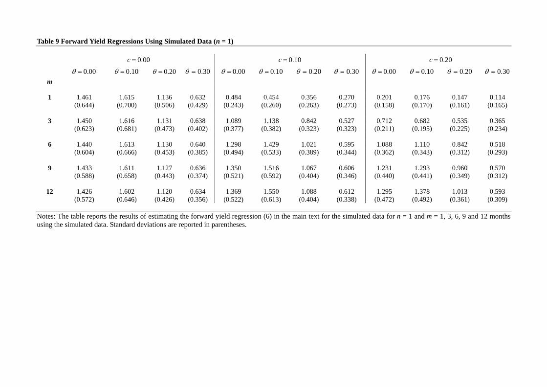
Table 9 Forward Yield Regressions Using Simulated Data (n = 1)

00.0=c 10.0=c 20.0=c

00.0=θ 10.0=θ 20.0=θ 30.0=θ 00.0=θ 10.0=θ 20.0=θ 30.0=θ 00.0=θ 10.0=θ 20.0=θ 30.0=θ m

1 1.461 1.615 1.136 0.632 0.484 0.454 0.356 0.270 0.201 0.176 0.147 0.114 (0.644) (0.700) (0.506) (0.429) (0.243) (0.260) (0.263) (0.273) (0.158) (0.170) (0.161) (0.165)

3 1.450 1.616 1.131 0.638 1.089 1.138 0.842 0.527 0.712 0.682 0.535 0.365 (0.623) (0.681) (0.473) (0.402) (0.377) (0.382) (0.323) (0.323) (0.211) (0.195) (0.225) (0.234)

6 1.440 1.613 1.130 0.640 1.298 1.429 1.021 0.595 1.088 1.110 0.842 0.518 (0.604) (0.666) (0.453) (0.385) (0.494) (0.533) (0.389) (0.344) (0.362) (0.343) (0.312) (0.293)

9 1.433 1.611 1.127 0.636 1.350 1.516 1.067 0.606 1.231 1.293 0.960 0.570 (0.588) (0.658) (0.443) (0.374) (0.521) (0.592) (0.404) (0.346) (0.440) (0.441) (0.349) (0.312)

12 1.426 1.602 1.120 0.634 1.369 1.550 1.088 0.612 1.295 1.378 1.013 0.593 (0.572) (0.646) (0.426) (0.356) (0.522) (0.613) (0.404) (0.338) (0.472) (0.492) (0.361) (0.309)

Notes: The table reports the results of estimating the forward yield regression (6) in the main text for the simulated data for n = 1 and m = 1, 3, 6, 9 and 12 months using the simulated data. Standard deviations are reported in parentheses.

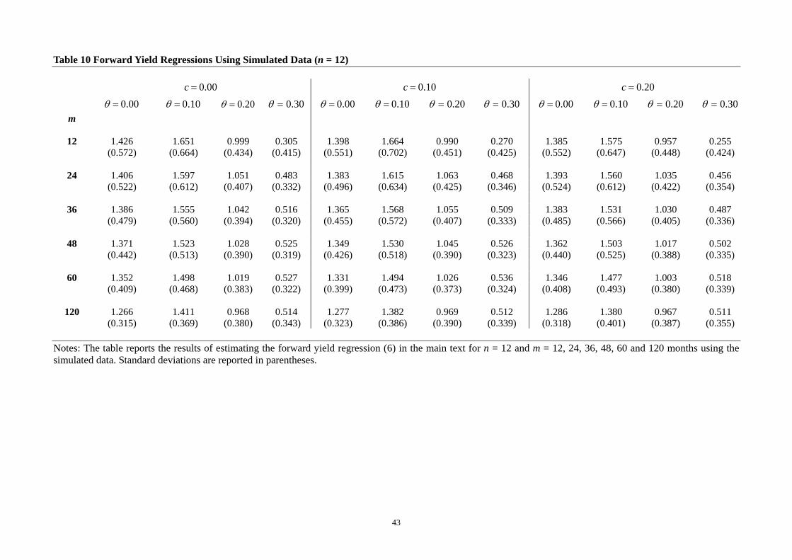
Table 10 Forward Yield Regressions Using Simulated Data (n = 12)

00.0=c 10.0=c 20.0=c

00.0=θ 10.0=θ 20.0=θ 30.0=θ 00.0=θ 10.0=θ 20.0=θ 30.0=θ 00.0=θ 10.0=θ 20.0=θ 30.0=θ m

12 1.426 1.651 0.999 0.305 1.398 1.664 0.990 0.270 1.385 1.575 0.957 0.255 (0.572) (0.664) (0.434) (0.415) (0.551) (0.702) (0.451) (0.425) (0.552) (0.647) (0.448) (0.424)

24 1.406 1.597 1.051 0.483 1.383 1.615 1.063 0.468 1.393 1.560 1.035 0.456 (0.522) (0.612) (0.407) (0.332) (0.496) (0.634) (0.425) (0.346) (0.524) (0.612) (0.422) (0.354)

36 1.386 1.555 1.042 0.516 1.365 1.568 1.055 0.509 1.383 1.531 1.030 0.487 (0.479) (0.560) (0.394) (0.320) (0.455) (0.572) (0.407) (0.333) (0.485) (0.566) (0.405) (0.336)

48 1.371 1.523 1.028 0.525 1.349 1.530 1.045 0.526 1.362 1.503 1.017 0.502 (0.442) (0.513) (0.390) (0.319) (0.426) (0.518) (0.390) (0.323) (0.440) (0.525) (0.388) (0.335)

60 1.352 1.498 1.019 0.527 1.331 1.494 1.026 0.536 1.346 1.477 1.003 0.518 (0.409) (0.468) (0.383) (0.322) (0.399) (0.473) (0.373) (0.324) (0.408) (0.493) (0.380) (0.339)

120 1.266 1.411 0.968 0.514 1.277 1.382 0.969 0.512 1.286 1.380 0.967 0.511 (0.315) (0.369) (0.380) (0.343) (0.323) (0.386) (0.390) (0.339) (0.318) (0.401) (0.387) (0.355)

Notes: The table reports the results of estimating the forward yield regression (6) in the main text for n = 12 and m = 12, 24, 36, 48, 60 and 120 months using the simulated data. Standard deviations are reported in parentheses.

43

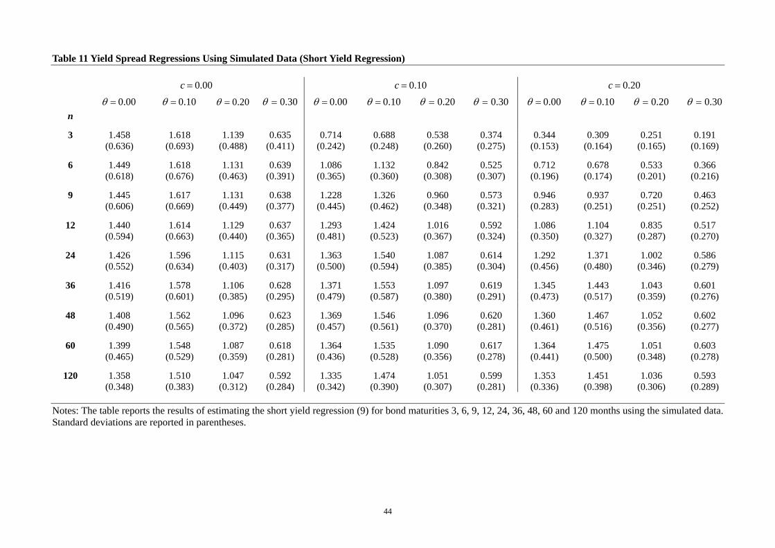
Table 11 Yield Spread Regressions Using Simulated Data (Short Yield Regression)

00.0=c 10.0=c 20.0=c

00.0=θ 10.0=θ 20.0=θ 30.0=θ 00.0=θ 10.0=θ 20.0=θ 30.0=θ 00.0=θ 10.0=θ 20.0=θ 30.0=θ n

3 1.458 1.618 1.139 0.635 0.714 0.688 0.538 0.374 0.344 0.309 0.251 0.191 (0.636) (0.693) (0.488) (0.411) (0.242) (0.248) (0.260) (0.275) (0.153) (0.164) (0.165) (0.169)

6 1.449 1.618 1.131 0.639 1.086 1.132 0.842 0.525 0.712 0.678 0.533 0.366 (0.618) (0.676) (0.463) (0.391) (0.365) (0.360) (0.308) (0.307) (0.196) (0.174) (0.201) (0.216)

9 1.445 1.617 1.131 0.638 1.228 1.326 0.960 0.573 0.946 0.937 0.720 0.463 (0.606) (0.669) (0.449) (0.377) (0.445) (0.462) (0.348) (0.321) (0.283) (0.251) (0.251) (0.252)

12 1.440 1.614 1.129 0.637 1.293 1.424 1.016 0.592 1.086 1.104 0.835 0.517 (0.594) (0.663) (0.440) (0.365) (0.481) (0.523) (0.367) (0.324) (0.350) (0.327) (0.287) (0.270)

24 1.426 1.596 1.115 0.631 1.363 1.540 1.087 0.614 1.292 1.371 1.002 0.586 (0.552) (0.634) (0.403) (0.317) (0.500) (0.594) (0.385) (0.304) (0.456) (0.480) (0.346) (0.279)

36 1.416 1.578 1.106 0.628 1.371 1.553 1.097 0.619 1.345 1.443 1.043 0.601 (0.519) (0.601) (0.385) (0.295) (0.479) (0.587) (0.380) (0.291) (0.473) (0.517) (0.359) (0.276)

48 1.408 1.562 1.096 0.623 1.369 1.546 1.096 0.620 1.360 1.467 1.052 0.602 (0.490) (0.565) (0.372) (0.285) (0.457) (0.561) (0.370) (0.281) (0.461) (0.516) (0.356) (0.277)

60 1.399 1.548 1.087 0.618 1.364 1.535 1.090 0.617 1.364 1.475 1.051 0.603 (0.465) (0.529) (0.359) (0.281) (0.436) (0.528) (0.356) (0.278) (0.441) (0.500) (0.348) (0.278)

120 1.358 1.510 1.047 0.592 1.335 1.474 1.051 0.599 1.353 1.451 1.036 0.593 (0.348) (0.383) (0.312) (0.284) (0.342) (0.390) (0.307) (0.281) (0.336) (0.398) (0.306) (0.289)

Notes: The table reports the results of estimating the short yield regression (9) for bond maturities 3, 6, 9, 12, 24, 36, 48, 60 and 120 months using the simulated data. Standard deviations are reported in parentheses.

44

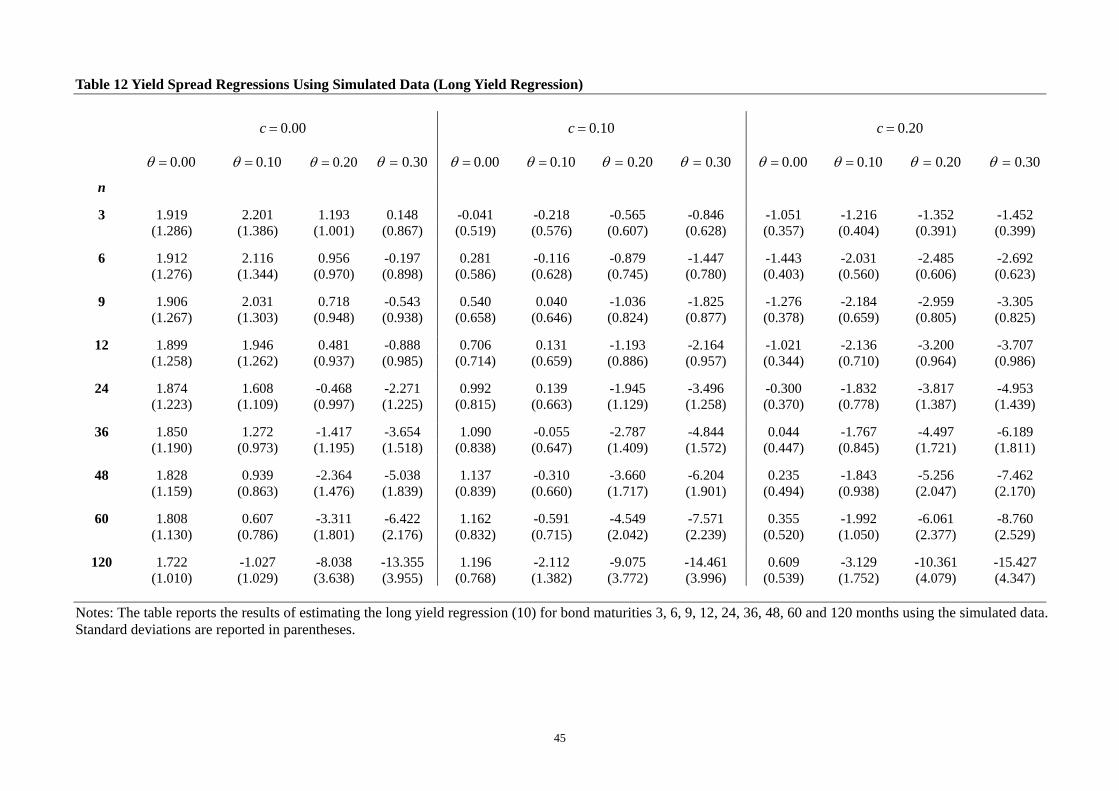
Table 12 Yield Spread Regressions Using Simulated Data (Long Yield Regression)

00.0=c 10.0=c 20.0=c

00.0=θ 10.0=θ 20.0=θ 30.0=θ 00.0=θ 10.0=θ 20.0=θ 30.0=θ 00.0=θ 10.0=θ 20.0=θ 30.0=θ

n

3 1.919 2.201 1.193 0.148 -0.041 -0.218 -0.565 -0.846 -1.051 -1.216 -1.352 -1.452 (1.286) (1.386) (1.001) (0.867) (0.519) (0.576) (0.607) (0.628) (0.357) (0.404) (0.391) (0.399)

6 1.912 2.116 0.956 -0.197 0.281 -0.116 -0.879 -1.447 -1.443 -2.031 -2.485 -2.692 (1.276) (1.344) (0.970) (0.898) (0.586) (0.628) (0.745) (0.780) (0.403) (0.560) (0.606) (0.623)

9 1.906 2.031 0.718 -0.543 0.540 0.040 -1.036 -1.825 -1.276 -2.184 -2.959 -3.305 (1.267) (1.303) (0.948) (0.938) (0.658) (0.646) (0.824) (0.877) (0.378) (0.659) (0.805) (0.825)

12 1.899 1.946 0.481 -0.888 0.706 0.131 -1.193 -2.164 -1.021 -2.136 -3.200 -3.707 (1.258) (1.262) (0.937) (0.985) (0.714) (0.659) (0.886) (0.957) (0.344) (0.710) (0.964) (0.986)

24 1.874 1.608 -0.468 -2.271 0.992 0.139 -1.945 -3.496 -0.300 -1.832 -3.817 -4.953 (1.223) (1.109) (0.997) (1.225) (0.815) (0.663) (1.129) (1.258) (0.370) (0.778) (1.387) (1.439)

36 1.850 1.272 -1.417 -3.654 1.090 -0.055 -2.787 -4.844 0.044 -1.767 -4.497 -6.189 (1.190) (0.973) (1.195) (1.518) (0.838) (0.647) (1.409) (1.572) (0.447) (0.845) (1.721) (1.811)

48 1.828 0.939 -2.364 -5.038 1.137 -0.310 -3.660 -6.204 0.235 -1.843 -5.256 -7.462 (1.159) (0.863) (1.476) (1.839) (0.839) (0.660) (1.717) (1.901) (0.494) (0.938) (2.047) (2.170)

60 1.808 0.607 -3.311 -6.422 1.162 -0.591 -4.549 -7.571 0.355 -1.992 -6.061 -8.760 (1.130) (0.786) (1.801) (2.176) (0.832) (0.715) (2.042) (2.239) (0.520) (1.050) (2.377) (2.529)

120 1.722 -1.027 -8.038 -13.355 1.196 -2.112 -9.075 -14.461 0.609 -3.129 -10.361 -15.427 (1.010) (1.029) (3.638) (3.955) (0.768) (1.382) (3.772) (3.996) (0.539) (1.752) (4.079) (4.347)

Notes: The table reports the results of estimating the long yield regression (10) for bond maturities 3, 6, 9, 12, 24, 36, 48, 60 and 120 months using the simulated data. Standard deviations are reported in parentheses.

45

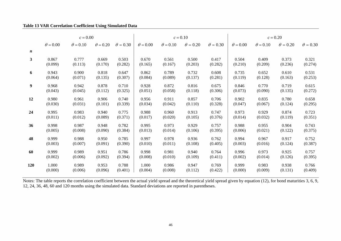
Table 13 VAR Correlation Coefficient Using Simulated Data

00.0=c 10.0=c 20.0=c

00.0=θ 10.0=θ 20.0=θ 30.0=θ 00.0=θ 10.0=θ 20.0=θ 30.0=θ 00.0=θ 10.0=θ 20.0=θ 30.0=θ n

3 0.867 0.777 0.669 0.503 0.670 0.561 0.500 0.417 0.504 0.409 0.373 0.321 (0.099) (0.113) (0.170) (0.282) (0.165) (0.167) (0.203) (0.282) (0.210) (0.209) (0.236) (0.274)

6 0.943 0.900 0.818 0.647 0.862 0.789 0.732 0.608 0.735 0.652 0.610 0.531 (0.064) (0.071) (0.135) (0.307) (0.084) (0.089) (0.137) (0.281) (0.119) (0.128) (0.163) (0.253)

9 0.968 0.942 0.878 0.710 0.928 0.872 0.816 0.675 0.846 0.770 0.719 0.615 (0.043) (0.045) (0.112) (0.325) (0.051) (0.058) (0.118) (0.306) (0.073) (0.090) (0.135) (0.272)

12 0.980 0.961 0.906 0.740 0.956 0.911 0.857 0.706 0.902 0.835 0.780 0.658 (0.030) (0.031) (0.101) (0.339) (0.034) (0.042) (0.110) (0.328) (0.047) (0.067) (0.124) (0.295)

24 0.995 0.983 0.940 0.775 0.988 0.960 0.913 0.747 0.973 0.929 0.874 0.723 (0.011) (0.012) (0.089) (0.371) (0.017) (0.020) (0.105) (0.376) (0.014) (0.032) (0.119) (0.351)

36 0.998 0.987 0.948 0.782 0.995 0.973 0.929 0.757 0.988 0.955 0.904 0.743 (0.005) (0.008) (0.090) (0.384) (0.013) (0.014) (0.106) (0.395) (0.006) (0.021) (0.122) (0.375)

48 0.999 0.988 0.950 0.785 0.997 0.978 0.936 0.762 0.994 0.967 0.917 0.752 (0.003) (0.007) (0.091) (0.390) (0.010) (0.011) (0.108) (0.405) (0.003) (0.016) (0.124) (0.387)

60 0.999 0.989 0.951 0.786 0.998 0.981 0.940 0.764 0.996 0.973 0.925 0.757 (0.002) (0.006) (0.092) (0.394) (0.008) (0.010) (0.109) (0.411) (0.002) (0.014) (0.126) (0.395)

120 1.000 0.989 0.953 0.788 1.000 0.986 0.947 0.769 0.999 0.983 0.938 0.766 (0.000) (0.006) (0.096) (0.401) (0.004) (0.008) (0.112) (0.422) (0.000) (0.009) (0.131) (0.409)

Notes: The table reports the correlation coefficient between the actual yield spread and the theoretical yield spread given by equation (12), for bond maturities 3, 6, 9, 12, 24, 36, 48, 60 and 120 months using the simulated data. Standard deviations are reported in parentheses.

46

Table 14 VAR Standard Deviation Ratio Using Simulated Data

00.0=c 10.0=c 20.0=c

00.0=θ 10.0=θ 20.0=θ 30.0=θ 00.0=θ 10.0=θ 20.0=θ 30.0=θ 00.0=θ 10.0=θ 20.0=θ 30.0=θ n

3 1.666 2.052 1.691 1.257 1.087 1.249 1.076 0.868 0.703 0.777 0.679 0.575 (0.663) (0.755) (0.534) (0.369) (0.311) (0.322) (0.264) (0.244) (0.168) (0.168) (0.168) (0.153)

6 1.526 1.775 1.354 0.934 1.272 1.447 1.127 0.796 0.992 1.064 0.859 0.636 (0.623) (0.692) (0.460) (0.317) (0.448) (0.492) (0.345) (0.275) (0.300) (0.299) (0.269) (0.217)

9 1.478 1.690 1.225 0.797 1.330 1.514 1.110 0.722 1.136 1.219 0.932 0.627 (0.604) (0.672) (0.436) (0.303) (0.498) (0.568) (0.377) (0.282) (0.381) (0.394) (0.327) (0.248)

12 1.451 1.653 1.156 0.719 1.351 1.546 1.088 0.669 1.211 1.311 0.962 0.607 (0.587) (0.660) (0.425) (0.300) (0.514) (0.603) (0.391) (0.286) (0.424) (0.455) (0.359) (0.264)

24 1.386 1.607 1.019 0.560 1.348 1.586 1.007 0.537 1.291 1.454 0.957 0.516 (0.520) (0.621) (0.392) (0.278) (0.491) (0.624) (0.390) (0.272) (0.452) (0.537) (0.383) (0.266)

36 1.339 1.594 0.937 0.474 1.317 1.594 0.941 0.458 1.285 1.497 0.909 0.447 (0.461) (0.586) (0.364) (0.253) (0.444) (0.600) (0.370) (0.248) (0.422) (0.540) (0.368) (0.247)

48 1.299 1.588 0.877 0.416 1.285 1.596 0.886 0.403 1.263 1.516 0.862 0.396 (0.412) (0.555) (0.342) (0.231) (0.399) (0.571) (0.351) (0.227) (0.385) (0.525) (0.350) (0.228)

60 1.266 1.585 0.829 0.374 1.256 1.596 0.840 0.363 1.240 1.527 0.821 0.358 (0.371) (0.527) (0.324) (0.214) (0.361) (0.543) (0.335) (0.210) (0.350) (0.505) (0.334) (0.212)

120 1.157 1.590 0.687 0.271 1.154 1.602 0.702 0.264 1.149 1.558 0.688 0.263 (0.242) (0.425) (0.276) (0.164) (0.236) (0.436) (0.287) (0.161) (0.233) (0.417) (0.285) (0.164)

Notes: The table reports the standard deviation ratio between the actual yield spread and the theoretical yield spread given by equation (12), for bond maturities 3, 6, 9, 12, 24, 36, 48, 60 and 120 months using the simulated data. Standard deviations are reported in parentheses.

47