Can computer vision problems benefit from structured

Machine Vision and ApplicationsDOI 10.1007/s00138-016-0763-9

SPECIAL ISSUE PAPER

Can computer vision problems benefit from structuredhierarchical classification?

Thomas Hoyoux1 · Antonio J. Rodríguez-Sánchez2 · Justus H. Piater2

Received: 8 December 2015 / Revised: 15 March 2016 / Accepted: 16 March 2016© The Author(s) 2016. This article is published with open access at Springerlink.com

Abstract Research in the field of supervised classificationhas mostly focused on the standard, so-called “flat” classifi-cation approach, where the problem classes live in a trivial,one-level semantic space. There is however an increasinginterest in the hierarchical classification approach, where aperformance gain is expected by incorporating prior taxo-nomic knowledge about the classes into the learning process.Intuitively, the hierarchical approach should be beneficial ingeneral for the classification of visual content, as suggestedby the fact that humans seem to organize objects into hierar-chies based on visually perceived similarities. In this paper,we provide an analysis that aims to determine the condi-tions under which the hierarchical approach can consistentlygive better performances than the flat approach for the clas-sification of visual content. In particular, we (1) show howhierarchical methods can fail to outperform flat methodswhen applied to real vision-based classification problems,and (2) investigate the underlying reasons for the lack ofimprovement, by applying the same methods to syntheticdatasets in a simulation. Our conclusion is that the use ofhigh-level hierarchical feature representations is crucial for

The research leading to these results has received funding from theEuropean Community’s Seventh Framework ProgrammeFP7/2007-2013 (Specific Programme Cooperation, Theme 3,Information and Communication Technologies) under GrantAgreements No. 270273, Xperience, and No. 600918, PaCMan.

B Thomas [email protected]

B Antonio J. Rodríguez-Sá[email protected]

1 Signal and Image Exploitation (INTELSIG), MontefioreInstitute, University of Liège, Liège, Belgium

2 Intelligent and Interactive Systems, Institute of ComputerScience, University of Innsbruck, Innsbruck, Austria

obtaining a performance gain with the hierarchical approach,and that poorly chosen prior taxonomies hinder this gain eventhough proper high-level features are used.

Keywords Hierarchical classification · Flat classification ·Structured K-nearest neighbors · Structured support vectormachines · Maximum margin regression ·3D shape classification ·Expression recognition · Simulationframework · Feature representations

1 Introduction

Most of the theoretical work and applications in the fieldof supervised classification have been dedicated to the stan-dard classification approach, where the problem classes areconsidered to be equally different fromeach other in a seman-tic sense [28]. In this standard approach, also known as“flat” classification, a classifier is learned from class-labeleddata instances without any explicit information given aboutthe high-level semantic relationships between the classes. Astandard multiclass problem formulation will for exampleconsider a bee, an ant and a hammer to be different to thesame degree; they belong to different classes in a flat sensebecause the only available semantic information comes fromthe same unique semantic level. However, one could considerthat ants and bees are part of a superclass of insects, whilehammers belong to another superclass of tools, and it is intu-itive that such hierarchical knowledge about the classes canhelp improve the classification performances. Based uponthis realization, a new approach has emerged for dealingmore efficiently with classification of content deemed tobe inherently semantically hierarchical, i.e., the hierarchicalclassification approach [28]. The attention given to the hier-archical approachwas also sustained by the advancesmade in

123

http://crossmark.crossref.org/dialog/?doi=10.1007/s00138-016-0763-9&domain=pdf

T. Hoyoux et al.

machine learning generalized to arbitrary output spaces, i.e.,the structured classification approach (e.g., [31]), of whichthe hierarchical approach is actually a special case.

The a priori hierarchical organization of classes has beenshown to constitute a key prior to classification problemsin several application domains, including text categorization[23], protein function prediction [7], and music genre classi-fication [14]. As for classification based on visual features,a hierarchical prior intuitively seems especially appropriateas it reflects the natural way in which humans organize andrecognize the objects they see, which is also supported byneurophysiological studies of the visual cortex [2,15,35].In practice, some results have shown that there is indeeda gain in performance with the hierarchical approach in thevisual-based application domain, e.g., for 3D object shapeclassification [3] and annotation of medical images [6]. Aquite active and closely related line of work consists of thesupervised construction of class hierarchies from imageswithmultiple tag labels. Themotivation is to reduce the com-plexity of visual recognition problems that have a very largenumber of instances. To build useful taxonomies, the pro-posed methods exploit either purely the semantic tag labels[19,29], or purely the visual information [10,18], or both asin [16], where the authors propose a way to learn a “seman-tivisual” hierarchy that is both semantically meaningful andclose to the visual content.

In this paper, we are interested in determining the condi-tions under which the hierarchical approach can consistentlygive better performances than the flat approach for the clas-sification of visual content. This paper is an extended versionof the work published in [11], where we applied three hier-archical classification methods and their flat counterpartsto two inherently hierarchical vision-based classificationproblems: facial expression recognition and 3D shape classi-fication. Using evaluationmeasures designed for hierarchicalclassification, we showed in [11] that, for the consideredmethods and problems, the hierarchical approach providednoor onlymarginal improvement over the standard approach.We here extend our previous work by designing a simula-tion framework and conducting the comparative evaluationof the hierarchical and flat methods used in [11] this timeapplied to artificial problems generated with this simulationframework. Specifically, we generate completely syntheticdatasets for which we can control the complexity through themanipulation of key aspects, such as the underlying hierar-chical phenomenon at the origin of the data measurements,the amount of noise in the extraction of the features fromthe measurements, and the amount of knowledge about theunderlying hierarchical phenomenon. Our goal with thesesimulation experiments is to draw useful insights to explainwhy the hierarchical approach did not outperform the flatapproach when applied to our real vision-based classifica-tion problems.

The remainder of this paper is organized as follows. Sec-tion 2 describes the hierarchical framework and terminologywe adopted for our previous and present work, and pro-vides the details of the hierarchical methods used. Section3 shows the experimental evaluation first presented in [11],where the hierarchical and flat methods were applied to realcomputer vision problems. Section 4 presents our simula-tion framework, as well as the experimental results obtainedfor artificial problems generated with this simulation frame-work. In light of the additional simulation results, we providea discussion in Sect. 5 and draw a conclusion in Sect. 6.

2 Methods for hierarchical classification

2.1 Framework and terminology

Recently, a necessary effort to unify the hierarchical classi-fication framework has been made [28]. We follow on theirterminology which is summarized next. A class taxonomyconsists of a finite set of semantic concepts C = {ci | i =1 . . . n} with a partial order relationship ≺ organizing theseconcepts either in a tree or a directed acyclic graph (DAG).A classification problem defined over such a taxonomy ishierarchical: its classes and superclasses correspond to theleaf and interior nodes of the tree (or DAG), respectively.A flat classification problem only considers the leaf nodesof such a taxonomy as its classes and has no superclass. Ahierarchical classification problem deals with either single-or multiple-path labeling, i.e., whether or not a single datainstance can be labeled with more than one path, and eitherfull or partial depth labeling, i.e., whether or not any path ina label must cover all hierarchy levels. In all cases, an indica-tor vector representation for the taxonomic label y of a datainstance can be used, i.e., y ∈ Y ⊂ {0, 1}n , where the i thcomponent of y takes value 1 if the data instance belongs tothe (super)class ci ∈ C, and 0 otherwise.

The real-world and simulation problems considered in thiswork are defined using tree taxonomies with full depth label-ing. For the facial expression recognition problem, we definemultiple path labeling (see Sect. 3.1.1), whereas for the 3Dshape classification problem and for our simulation problemswe define single path labeling (see Sects. 3.2.1 and 4.2).

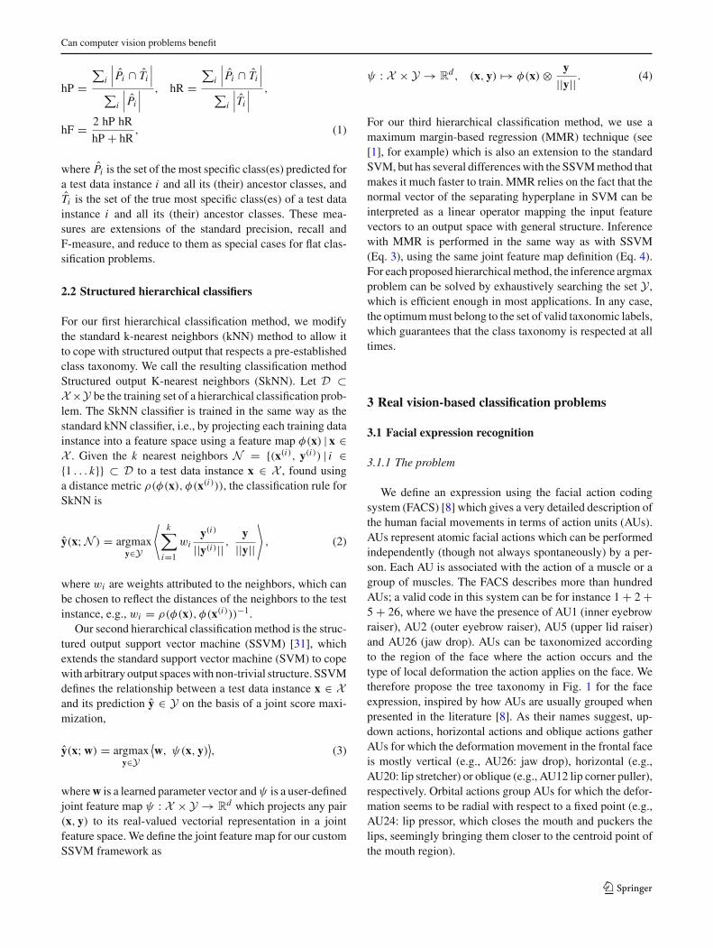
Because they do not penalize structural errors, evaluationmeasures used in the standard flat classification approachmay not be appropriate when comparing hierarchical meth-ods to each other, or flat methods to hierarchical methods. Inparticular, they do not consider that misclassification at dif-ferent levels of the taxonomy should be treated in differentways. In this work, we adopt the following measures [12],also recommended by [28]: hierarchical precision (hP), hier-archical recall (hR) and hierarchical F-measure (hF), definedas

123

Can computer vision problems benefit

hP =∑

i

∣∣∣Pi ∩ Ti

∣∣∣

∑i

∣∣∣Pi

∣∣∣

, hR =∑

i

∣∣∣Pi ∩ Ti

∣∣∣

∑i

∣∣∣Ti

∣∣∣

,

hF = 2 hP hR

hP + hR, (1)

where Pi is the set of the most specific class(es) predicted fora test data instance i and all its (their) ancestor classes, andTi is the set of the true most specific class(es) of a test datainstance i and all its (their) ancestor classes. These mea-sures are extensions of the standard precision, recall andF-measure, and reduce to them as special cases for flat clas-sification problems.

2.2 Structured hierarchical classifiers

For our first hierarchical classification method, we modifythe standard k-nearest neighbors (kNN) method to allow itto cope with structured output that respects a pre-establishedclass taxonomy. We call the resulting classification methodStructured output K-nearest neighbors (SkNN). Let D ⊂X ×Y be the training set of a hierarchical classification prob-lem. The SkNN classifier is trained in the same way as thestandard kNN classifier, i.e., by projecting each training datainstance into a feature space using a feature map φ(x) | x ∈X . Given the k nearest neighbors N = {(x(i), y(i)) | i ∈{1 . . . k}} ⊂ D to a test data instance x ∈ X , found usinga distance metric ρ(φ(x), φ(x(i))), the classification rule forSkNN is

y(x;N ) = argmaxy∈Y

⟨k∑

i=1

wiy(i)

||y(i)|| ,y

||y||

⟩

, (2)

where wi are weights attributed to the neighbors, which canbe chosen to reflect the distances of the neighbors to the testinstance, e.g., wi = ρ(φ(x), φ(x(i)))−1.

Our second hierarchical classification method is the struc-tured output support vector machine (SSVM) [31], whichextends the standard support vector machine (SVM) to copewith arbitrary output spaceswith non-trivial structure. SSVMdefines the relationship between a test data instance x ∈ Xand its prediction y ∈ Y on the basis of a joint score maxi-mization,

y(x;w) = argmaxy∈Y

⟨w, ψ(x, y)

⟩, (3)

wherew is a learned parameter vector andψ is a user-definedjoint feature map ψ : X × Y → R

d which projects any pair(x, y) to its real-valued vectorial representation in a jointfeature space. We define the joint feature map for our customSSVM framework as

ψ : X × Y → Rd , (x, y) �→ φ(x) ⊗ y

||y|| . (4)

For our third hierarchical classification method, we use amaximum margin-based regression (MMR) technique (see[1], for example) which is also an extension to the standardSVM, but has several differenceswith the SSVMmethod thatmakes it much faster to train. MMR relies on the fact that thenormal vector of the separating hyperplane in SVM can beinterpreted as a linear operator mapping the input featurevectors to an output space with general structure. Inferencewith MMR is performed in the same way as with SSVM(Eq. 3), using the same joint feature map definition (Eq. 4).For each proposed hierarchicalmethod, the inference argmaxproblem can be solved by exhaustively searching the set Y ,which is efficient enough in most applications. In any case,the optimummust belong to the set of valid taxonomic labels,which guarantees that the class taxonomy is respected at alltimes.

3 Real vision-based classification problems

3.1 Facial expression recognition

3.1.1 The problem

We define an expression using the facial action codingsystem (FACS) [8] which gives a very detailed description ofthe human facial movements in terms of action units (AUs).AUs represent atomic facial actions which can be performedindependently (though not always spontaneously) by a per-son. Each AU is associated with the action of a muscle or agroup of muscles. The FACS describes more than hundredAUs; a valid code in this system can be for instance 1 + 2 +5 + 26, where we have the presence of AU1 (inner eyebrowraiser), AU2 (outer eyebrow raiser), AU5 (upper lid raiser)and AU26 (jaw drop). AUs can be taxonomized accordingto the region of the face where the action occurs and thetype of local deformation the action applies on the face. Wetherefore propose the tree taxonomy in Fig. 1 for the faceexpression, inspired by how AUs are usually grouped whenpresented in the literature [8]. As their names suggest, up-down actions, horizontal actions and oblique actions gatherAUs for which the deformation movement in the frontal faceis mostly vertical (e.g., AU26: jaw drop), horizontal (e.g.,AU20: lip stretcher) or oblique (e.g., AU12 lip corner puller),respectively. Orbital actions group AUs for which the defor-mation seems to be radial with respect to a fixed point (e.g.,AU24: lip pressor, which closes the mouth and puckers thelips, seemingly bringing them closer to the centroid point ofthe mouth region).

123

T. Hoyoux et al.

Fig. 1 Our facial expression taxonomy. The leaves (classes) correspond to Action Units

3.1.2 The extended Cohn–Kanade dataset (CK+)

The CK+ dataset [17] consists of 123 subjects between theage of 18 and 50 years, of which 69% are female, 81%Euro-American, 13%Afro-American, and 6% other groups.Subjects were instructed to perform a series of 23 facial dis-plays. In total, 593 videos of 10–60 frames were recordedand annotated with an expression label in the form of anFACS code. All videos start with an onset neutral expres-sion and end with the peak of the expression that the subjectwas asked to display. Additionally, landmark annotations areprovided for all frames of all videos: 68 fiducial points havebeen marked on the face, sketching the most salient parts ofthe face shape.

3.1.3 Face features

Weuse face features very similar to the similarity normalizedshape features (SPTS) and canonical normalized appearancefeatures (CAPP) used in [17]. On the CK+ dataset, our fea-tures for a video consist of a 636-dimensional real-valuedvector extracted from the peak expression frame of thatvideo. 136 elements are encoding information about the faceshape, while 500 elements encode information about the faceappearance. We chose to subtract the onset frame data fromthe peak frame data, like it was done in [17], to avoid mix-ing our expression recognition problem with an unwantedidentity component embodying static morphological differ-ences. For that reason, the face features we use can be called“identity-normalized”.

3.1.4 Results

The three hierarchical classification methods of interest, i.e.,SkNN, SSVM and MMR, are compared to their flat coun-terparts: kNN, Multiclass Kernel-based Vector Machines(MKSVM [5]) and “flat setup”MMR, i.e.,MMRnot exploit-ing the hierarchical information. For each tested method,

there exists a main parameter, the tuning of which can havehuge influence on the results. For SkNN and kNN, this para-meter is the number of neighbors to consider during the testphase. For SSVM and MKSVM, the core parameter is thetraining parameter “C”, which, in the soft-margin approach,balances the allowed misclassification rate during the train-ing procedure. We found empirically that, for MMR, usinga polynomial kernel brings the best performances (whereasfor SSVM andMKSVMwe use a linear kernel), and the coreparameter for MMR is therefore the degree of this polyno-mial kernel.

Figure 2 shows the hierarchical F-measure (hF) curvesobtained for the facial expression recognition task. Globally,we can observe that hierarchical classification does not seemto outperform flat classification with either of the proposedhierarchical methods. Having a closer look at the highestpoints from each of those performance curves, i.e., the pointswith the best hF (Table 1), we can see that the flat and hier-archical approaches give very similar performances for thisexpression recognition problem.

3.2 3D shape classification

3.2.1 The problem

Given a tree taxonomy of 3D objects such as the one pre-sented in Fig. 3, the task is to determine to which class anew object instance belongs, based on its 3D shape featurerepresentation.

3.2.2 The princeton shape benchmark (PSB)

The PSB dataset (Fig. 3) [27] is one of the largest and mostheterogeneous datasets of 3Dobjects: 1814 3Dmodels corre-sponding to a wide variety of natural and man-made objectsare grouped into 161 classes. Thesemodels encode the polyg-onal geometry of the object they describe. The groupingwas based not only on semantic and functional concepts

123


10 20 30 400.4

0.5

0.6

0.7

0.8

0.9

1

neighbors

hFEXPR−SkNNEXPR−kNN

0 5000 100000.4

0.5

0.6

0.7

0.8

0.9

1

C

hF

EXPR−SSVMEXPR−MKSVM

20 40 600.4

0.5

0.6

0.7

0.8

0.9

1

polynomial degree

hF

EXPR−MMR (hier.)EXPR−MMR (flat)

Fig. 2 Facial expression recognition results. Blue and red curves showhF for hierarchical and flat classification respectively, against the num-ber of neighbors for SkNN vs. kNN (left), the “C” parameter for SSVMvs. MKSVM (center), and the degree of the polynomial kernel for hier-archical vs. flat setup MMR (right)

Table 1 Best hF performances from Fig. 2, along with the corre-sponding hP and hR performances obtained for the facial expressionrecognition task

hP (%) hR (%) hF (%)

SkNN 83.63 88.00 85.76

kNN 83.12 87.98 85.48

SSVM 85.22 87.87 86.52

MKSVM 85.68 87.54 86.60

MMR (hier.) 85.84 87.76 86.79

MMR (flat) 86.46 88.07 87.26

(e.g., “furniture” is a superclass of “table”) but also on shapeattributes (e.g., round tables belong to the same class).

3.2.3 3D shape descriptors

Each object instance is encoded into a point cloud which issampled from its original mesh file: 5000 points from thetriangulated surface, where the probability of a point beingselected from a triangle is related to the area of the trian-gle that contains it. From this sampling, we calculate five3D descriptors for each object: ensemble of shape functions(ESF) [34], viewpoint feature histogram (VFH) [24], intrinsicspin images (SI) [32], signature of histograms of orientations(SHOT) [30] and unique shape contexts (USC) [4]). Thereasons for choosing those descriptors are (1) uniqueness(preference to heterogeneity of algorithms) and (2) accessi-bility (the methods used are available from the point cloudlibrary [25]). By applying our methods to different descrip-tors, we wish to multiply the classification experiments toenhance our comparison between hierarchical and flat meth-ods for the 3D shape classification problem.

3.2.4 Results

We perform 3D shape classification with each of the fivedescriptors, i.e., ESF,VFH,SI, SHOTandUSC, using eachof

the three hierarchical classification methods of interest, i.e.,SkNN, SSVM and MMR, as well as their flat counterparts,i.e., kNN, MKSVM and “flat setup” MMR. Again, we makethe most influential parameter for each method vary in ourtests; those are the number of neighbors for SkNN and kNN,the “C” parameter for SSVM and MKSVM, and the degreeof the polynomial kernel for MMR.

Figure 4 shows the hierarchical F-measure (hF) curvesobtained for all test cases. There seems to be, for some ofthe five descriptors, a consistent yet very slight trend show-ing some performance improvement when using hierarchicalclassification. Indeed, the VFH and ESF descriptors seemto benefit a little from hierarchical information in all threemethods, as it is further illustrated in Table 2 which givesdetails about the best hF values obtained for all test cases.For SI, SHOT and USC descriptors, results are mixed: eitherhierarchical or flat classification performs slightly better,depending on the method. Again, hierarchical classificationdoes not clearly appear to give better results than flat classi-fication but for a few cases.

4 Artificial classification problems

4.1 Motivation

The results presented in Sect. 3 for real-world problems arenot easy to interpret. After systematically applying three dif-ferent hierarchical classification methods to two differentvision-based problems with several different types of fea-tures,we failed to showcase the superiority of the hierarchicalapproach over the flat one for classification based on visualfeatures. However, as stated in Sect. 1, such superiority (1)has been demonstrated in general in other fields, such as textcategorization and protein function prediction, and (2) wouldhave been expected as suggested by neurophysiological stud-ies of the visual cortex.

In our previous work, we hypothesized that the featureswe used, which are commonly used in 2D and 3D computervision for general purpose, might lack the information neces-sary to exploit a hierarchical prior. Based on that hypothesis,we can ask ourselves three further questions about the under-lying causes:

1. Do the features fail to capture any hierarchical informa-tion by nature?

2. Do the features capture hierarchical information struc-turally different from the hierarchical prior?

3. Do the features capture hierarchical information struc-turally similar to the hierarchical prior, with so muchnoise that our hierarchical methods fail?

123

T. Hoyoux et al.

Fig. 3 The “Furniture” and “animal” sub-trees of the Princeton Shape Benchmark, with snapshots of some of the models that belong to the leaves(classes) of those sub-trees

0 20 400

0.1

0.2

0.3

0.4

0.5

neighbors

hF

ESF−SkNNESF−kNN

0 20 400

0.1

0.2

0.3

0.4

0.5

neighbors

hF

VFH−SkNNVFH−kNN

0 20 400

0.1

0.2

0.3

0.4

0.5

neighbors

hF

SI−SkNNSI−kNN

0 20 400

0.1

0.2

0.3

0.4

0.5

neighbors

hFSHOT−SkNNSHOT−kNN

0 20 400

0.1

0.2

0.3

0.4

0.5

neighbors

hF

USC−SkNNUSC−kNN

0 5 10x 104

0

0.1

0.2

0.3

0.4

0.5

C

hF

ESF−SSVMESF−MKSVM

0 5 10x 104

0

0.1

0.2

0.3

0.4

0.5

C

hF

VFH−SSVMVFH−MKSVM

0 5 10x 104

0

0.1

0.2

0.3

0.4

0.5

C

hF

SI−SSVMSI−MKSVM

0 5 10x 104

0

0.1

0.2

0.3

0.4

0.5

C

hF

SHOT−SSVMSHOT−MKSVM

0 5 10x 104

0

0.1

0.2

0.3

0.4

0.5

C

hF

USC−SSVMUSC−MKSVM

20 40 60 800

0.1

0.2

0.3

0.4

0.5

polynomial degree

hF

ESF−MMR (hier.)ESF−MMR (flat)

20 40 60 800

0.1

0.2

0.3

0.4

0.5

polynomial degree

hF

VFH−MMR (hier.)VFH−MMR (flat)

20 40 60 800

0.1

0.2

0.3

0.4

0.5

polynomial degree

hF

SI−MMR (hier.)SI−MMR (flat)

20 40 60 800

0.1

0.2

0.3

0.4

0.5

polynomial degree

hF

SHOT−MMR (hier.)SHOT−MMR (flat)

20 40 60 800

0.1

0.2

0.3

0.4

0.5

polynomial degree

hF

USC−MMR (hier.)USC−MMR (flat)

Fig. 4 3D shape classification results. Blue and red curves show hFfor hierarchical and flat classification respectively, against the numberof neighbors for SkNN vs. kNN in the first row, the “C” parameter forSSVM vs. MKSVM in the second row and the degree of the polyno-

mial kernel for MMR (hierarchical vs. flat setup) in the third row. Eachcolumn corresponds to the use of a particular descriptor: ESF, VFH, SI,SHOT and USC

123


Table 2 Best hF performancesfrom Fig. 4, along with thecorresponding hP and hRperformances obtained for the3D shape classification taskusing the shape descriptors ESF,VFH, SI, SHOT and USC

Measure ESF VFH SI SHOT USC

SkNN hP (%) 32.23 20.38 27.24 34.36 40.26

hR (%) 34.40 23.07 29.07 34.95 41.08

hF (%) 33.28 21.64 28.12 34.65 40.67

kNN hP (%) 32.00 19.60 26.42 33.99 40.78

hR (%) 34.22 21.42 27.79 35.48 41.18

hF (%) 33.07 20.47 27.09 34.72 40.98

SSVM hP (%) 49.72 23.47 31.15 33.43 37.58

hR (%) 49.92 23.62 33.58 36.35 40.88

hF (%) 49.82 23.55 32.32 34.83 39.16

MKSVM hP (%) 47.78 21.84 31.01 35.79 37.56

hR (%) 47.45 21.84 32.23 36.67 39.41

hF (%) 47.61 21.84 31.61 36.22 38.46

MMR (hier. setup) hP (%) 45.56 24.70 26.07 30.35 28.40

hR (%) 44.93 24.44 26.57 31.86 30.53

hF (%) 45.24 24.57 26.32 31.09 29.43

MMR (flat setup) hP (%) 44.72 23.63 26.05 28.98 29.96

hR (%) 45.02 23.62 26.62 30.03 31.70

hF (%) 44.87 23.62 26.33 29.50 30.81

To give answers to these rather general questions, webelieve that it is a good strategy to not focus into a spe-cific problem but instead consider a general approach. Todo so, we have designed a simulation framework whichgenerates abstract, artificial classification problems, the com-plexity of which can be controlled through the manipulationof key aspects for hierarchical classification. From the resultsobtained with our hierarchical and flat classificationmethodsapplied to these artificial problems, we wish to draw usefulinsights about the conditions under which the hierarchicalapproach can offer a real gain in performance.

4.2 Simulation framework

4.2.1 Abstraction of the classification problem

To build a meaningful simulation framework, we need tohave a clear view of the concepts at work in the hierarchicaland flat classification approaches (Fig. 5). In abstract terms,the repeated manifestation of a phenomenon is measured bya sensor on one hand, and a semantic classification of thepossible states of the phenomenon made by an observer onthe other hand. We are interested in phenomena that havea natural hierarchical relationship between their states, i.e.,an underlying taxonomy.1 Being aware of the hierarchicalnature of a phenomenon, the observer may organize the

1 It is arguable whether or not there exists such a thing as an “under-lying taxonomy” for a phenomenon; taxonomies may be thought of asalways being arbitrary, their value lying in their usefulness, not in someunderlying, self-evident truth.

Fig. 5 Schematic view of the hierarchical and flat classificationapproaches used in our simulation framework

semantic classes in a hierarchical manner, i.e., define a per-ceived taxonomy. This perceived taxonomy does howevernot necessarily correspond perfectly to the natural underly-ing taxonomy.

123

T. Hoyoux et al.

The semantic classes provided by the observer are thenused to label a collection ofmeasurements, yielding a labeleddataset. At the same time, a feature extraction method isapplied to the collection of measurements, with the primarygoal of capturing the essential characteristics present in thedata for a supervised classification task. If we assume thatthe measurements contain information about the underlyingtaxonomy of the phenomenon,2 a so-called high-level fea-ture extraction should be able to capture at least part of thisessential information, while low-level feature extraction islikely to fail to capture any of it.

A set of labeled features is therefore available for learninga classifier, i.e., a machine that predicts the class associatedwith new measurements of the same phenomenon, on thebasis of features extracted using the same feature extractionmethod. To evaluate the generalization capability of a classi-fier, the set is split into a training and a test set. The trainingof a hierarchical classifier differs from the training of a flatone by the fact that the hierarchical learning method is giventhe perceived taxonomy as a prior, whereas the flat learningmethod does not make use of a hierarchical prior about theclasses.

Making use or not of a hierarchical prior during learn-ing, all other things remaining equal, the classificationperformances of the hierarchical and flat classifiers can becompared on the basis of the perceived taxonomy which, inthis case, is used as a hierarchical penalty criterion for themisclassification of the elements of the test set (e.g., usingthe hierarchical F-measure, see Sect. 2.1). Indeed, for bothtypes of classifiers, the superclasses come as a byproductof the predicted class according to a given taxonomy, andthose superclasses can be used to penalize misclassificationof examples, making emphasis on serious hierarchical errorsaccording to the given taxonomy.

4.2.2 Artificial datasets with taxonomies

Following on what has been discussed in Sect. 4.2.1, we areinterested in generating datasets obtained from phenomenawith underlying taxonomies. To simulate such taxonomies,we consider perfect k-ary trees, where all leaf nodes are atthe same level L (the root is at the level 1) and all internalnodes have degree k, i.e., k children. For such trees, the total

number of nodes is given by kL−1k−1 , and the number of leaf

nodes is kL−1. In our view, a path from the root to a leafnode of such a taxonomy corresponds to a state of the hier-archical phenomenon that is being measured by the sensorand interpreted by the observer. Note that we do not considerproblems where a single manifestation of a phenomenon can

2 The measurements may comply particularly well to a specific tax-onomic model, that would be the best, i.e., most useful taxonomicapproximation of the nature of the phenomenon.

Table 3 Underlying taxonomies of the phenomena under considerationin our simulation experiments

k L #nodes #leaves (classes)

Binary trees 2 3 7 4

2 4 15 8

2 5 31 16

2 6 63 32

2 7 127 64

Ternary trees 3 3 13 9

3 4 40 27

3 5 121 81

Quadtrees 4 3 21 16

4 4 85 64

simultaneously correspond to multiple paths in the underly-ing tree taxonomy.We consider 10 different phenomena withsuch underlying taxonomies (see Table 3). For each phenom-enon, we assume (1) that the observer was able to establishthe existence of all the different states and make them cor-respond to semantic classes, and (2) that 200 manifestationsper state were measured by the sensor and correctly class-labeled by the observer. We then have 10 labeled datasetswhich are perfectly class-balanced.

In our view, the observer has also established a per-ceived taxonomy embodying the hierarchical relationshipsbetween the semantic classes. For each dataset, we con-sider a first experimental simulation condition where theperceived taxonomy perfectly matches the actual underlyingtaxonomy of the phenomenon associated with this dataset.We also consider a second simulation condition where theperceived taxonomy does not match the underlying one atdifferent degrees. The artificial problems generated with thissecond condition simulate real problems where the chosentaxonomies are arbitrary and do not optimally reflect thehierarchical nature of the phenomenon. To test this secondsimulation condition, we focus on the dataset associated withthe underlyingbinary tree taxonomywith 7 levels (127nodes,64 leaves).

4.2.3 Artificial high-level features

We assume that the measurements in our datasets somehowencode the underlying hierarchical nature of the phenom-enon, which applies in most practical cases. For each dataset,we simulate a series of high-level feature extractions withdifferent levels of noise. More precisely, a combination of adataset and a noise level yields a unique classification prob-lem involving the noisy features and the class labels for thisdataset (as well as the perceived taxonomy as a prior whenhierarchical classification is considered).

123


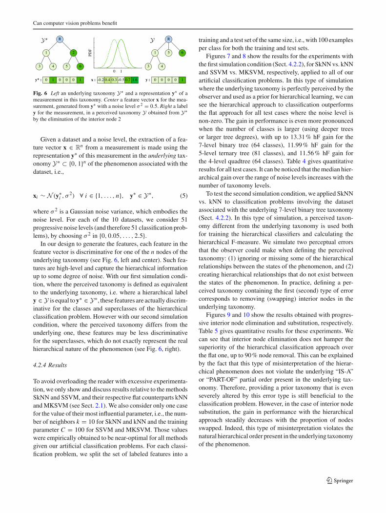
Fig. 6 Left an underlying taxonomy Y∗ and a representation y∗ of ameasurement in this taxonomy. Center a feature vector x for the mea-surement, generated from y∗ with a noise level σ 2 = 0.5. Right a labely for the measurement, in a perceived taxonomy Y obtained from Y∗by the elimination of the interior node 2

Given a dataset and a noise level, the extraction of a fea-ture vector x ∈ R

n from a measurement is made using therepresentation y∗ of this measurement in the underlying tax-onomy Y∗ ⊂ {0, 1}n of the phenomenon associated with thedataset, i.e.,

xi ∼ N (y∗i , σ

2) ∀ i ∈ {1, . . . , n}, y∗ ∈ Y∗, (5)

where σ 2 is a Gaussian noise variance, which embodies thenoise level. For each of the 10 datasets, we consider 51progressive noise levels (and therefore 51 classification prob-lems), by choosing σ 2 in {0, 0.05, . . . , 2.5}.

In our design to generate the features, each feature in thefeature vector is discriminative for one of the n nodes of theunderlying taxonomy (see Fig. 6, left and center). Such fea-tures are high-level and capture the hierarchical informationup to some degree of noise. With our first simulation condi-tion, where the perceived taxonomy is defined as equivalentto the underlying taxonomy, i.e. where a hierarchical labely ∈ Y is equal toy∗ ∈ Y∗, these features are actually discrim-inative for the classes and superclasses of the hierarchicalclassification problem. However with our second simulationcondition, where the perceived taxonomy differs from theunderlying one, these features may be less discriminativefor the superclasses, which do not exactly represent the realhierarchical nature of the phenomenon (see Fig. 6, right).

4.2.4 Results

To avoid overloading the reader with excessive experimenta-tion, we only show and discuss results relative to themethodsSkNN and SSVM, and their respective flat counterparts kNNandMKSVM (see Sect. 2.1). We also consider only one casefor the value of their most influential parameter, i.e., the num-ber of neighbors k = 10 for SkNN and kNN and the trainingparameter C = 100 for SSVM and MKSVM. Those valueswere empirically obtained to be near-optimal for all methodsgiven our artificial classification problems. For each classi-fication problem, we split the set of labeled features into a

training and a test set of the same size, i.e., with 100 examplesper class for both the training and test sets.

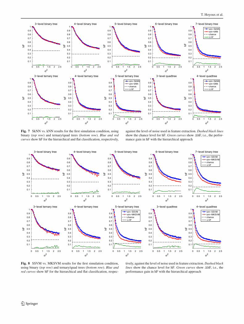
Figures 7 and 8 show the results for the experiments withthe first simulation condition (Sect. 4.2.2), for SkNNvs. kNNand SSVM vs. MKSVM, respectively, applied to all of ourartificial classification problems. In this type of simulationwhere the underlying taxonomy is perfectly perceived by theobserver and used as a prior for hierarchical learning, we cansee the hierarchical approach to classification outperformsthe flat approach for all test cases where the noise level isnon-zero. The gain in performance is even more pronouncedwhen the number of classes is larger (using deeper treesor larger tree degrees), with up to 13.31% hF gain for the7-level binary tree (64 classes), 11.99% hF gain for the5-level ternary tree (81 classes), and 11.56% hF gain forthe 4-level quadtree (64 classes). Table 4 gives quantitativeresults for all test cases. It can be noticed that themedian hier-archical gain over the range of noise levels increases with thenumber of taxonomy levels.

To test the second simulation condition, we applied SkNNvs. kNN to classification problems involving the datasetassociated with the underlying 7-level binary tree taxonomy(Sect. 4.2.2). In this type of simulation, a perceived taxon-omy different from the underlying taxonomy is used bothfor training the hierarchical classifiers and calculating thehierarchical F-measure. We simulate two perceptual errorsthat the observer could make when defining the perceivedtaxonomy: (1) ignoring or missing some of the hierarchicalrelationships between the states of the phenomenon, and (2)creating hierarchical relationships that do not exist betweenthe states of the phenomenon. In practice, defining a per-ceived taxonomy containing the first (second) type of errorcorresponds to removing (swapping) interior nodes in theunderlying taxonomy.

Figures 9 and 10 show the results obtained with progres-sive interior node elimination and substitution, respectively.Table 5 gives quantitative results for these experiments. Wecan see that interior node elimination does not hamper thesuperiority of the hierarchical classification approach overthe flat one, up to 90% node removal. This can be explainedby the fact that this type of misinterpretation of the hierar-chical phenomenon does not violate the underlying “IS-A”or “PART-OF” partial order present in the underlying tax-onomy. Therefore, providing a prior taxonomy that is evenseverely altered by this error type is still beneficial to theclassification problem. However, in the case of interior nodesubstitution, the gain in performance with the hierarchicalapproach steadily decreases with the proportion of nodesswapped. Indeed, this type of misinterpretation violates thenatural hierarchical order present in the underlying taxonomyof the phenomenon.

123

T. Hoyoux et al.

0 0.5 1 1.5 2 2.5

0.1

0.2

0.3

0.4

0.5

0.6

0.7

0.8

0.9

13−level binary tree

σ2

hF

0 0.5 1 1.5 2 2.5

0.1

0.2

0.3

0.4

0.5

0.6

0.7

0.8

0.9


σ2

hF0 0.5 1 1.5 2 2.5

0.1

0.2

0.3

0.4

0.5

0.6

0.7

0.8

0.9


σ2

hF

0 0.5 1 1.5 2 2.5

0.1

0.2

0.3

0.4

0.5

0.6

0.7

0.8

0.9


σ2

hF

0 0.5 1 1.5 2 2.5

0.1

0.2

0.3

0.4

0.5

0.6

0.7

0.8

0.9


σ2

hF

sim−SkNNsim−kNNchanceΔ hF

0 0.5 1 1.5 2 2.5

0.1

0.2

0.3

0.4

0.5

0.6

0.7

0.8

0.9

13−level ternary tree

σ2

hF

0 0.5 1 1.5 2 2.5

0.1

0.2

0.3

0.4

0.5

0.6

0.7

0.8

0.9


σ2

hF

0 0.5 1 1.5 2 2.5

0.1

0.2

0.3

0.4

0.5

0.6

0.7

0.8

0.9


σ2

hF


0 0.5 1 1.5 2 2.5

0.1

0.2

0.3

0.4

0.5

0.6

0.7

0.8

0.9

13−level quadtree

σ2

hF

0 0.5 1 1.5 2 2.5

0.1

0.2

0.3

0.4

0.5

0.6

0.7

0.8

0.9

14−level quadtree

σ2

hF


Fig. 7 SkNN vs. kNN results for the first simulation condition, usingbinary (top row) and ternary/quad trees (bottom row). Blue and redcurves show hF for the hierarchical and flat classification, respectively,

against the level of noise used in feature extraction. Dashed black linesshow the chance level for hF. Green curves show �hF, i.e., the perfor-mance gain in hF with the hierarchical approach

0 0.5 1 1.5 2 2.5

0.1

0.2

0.3

0.4

0.5

0.6

0.7

0.8

0.9


σ2

hF

0 0.5 1 1.5 2 2.5

0.1

0.2

0.3

0.4

0.5

0.6

0.7

0.8

0.9


σ2

hF

0 0.5 1 1.5 2 2.5

0.1

0.2

0.3

0.4

0.5

0.6

0.7

0.8

0.9


σ2

hF

0 0.5 1 1.5 2 2.5

0.1

0.2

0.3

0.4

0.5

0.6

0.7

0.8

0.9


σ2

hF

0 0.5 1 1.5 2 2.5

0.1

0.2

0.3

0.4

0.5

0.6

0.7

0.8

0.9


σ2

hF

sim−SSVMsim−MKSVMchanceΔ hF

0 0.5 1 1.5 2 2.5

0.1

0.2

0.3

0.4

0.5

0.6

0.7

0.8

0.9


σ2

hF

0 0.5 1 1.5 2 2.5

0.1

0.2

0.3

0.4

0.5

0.6

0.7

0.8

0.9


σ2

hF

0 0.5 1 1.5 2 2.5

0.1

0.2

0.3

0.4

0.5

0.6

0.7

0.8

0.9


σ2

hF


0 0.5 1 1.5 2 2.5

0.1

0.2

0.3

0.4

0.5

0.6

0.7

0.8

0.9

13−level quadtree

σ2

hF

0 0.5 1 1.5 2 2.5

0.1

0.2

0.3

0.4

0.5

0.6

0.7

0.8

0.9

14−level quadtree

σ2

hF


Fig. 8 SSVM vs. MKSVM results for the first simulation condition,using binary (top row) and ternary/quad trees (bottom row). Blue andred curves show hF for the hierarchical and flat classification, respec-

tively, against the level of noise used in feature extraction.Dashed blacklines show the chance level for hF. Green curves show �hF, i.e., theperformance gain in hF with the hierarchical approach

123


Table 4 Median and maximal �hF, i.e., performance gains in hF with the hierarchical approach, in our results for the first simulation conditionshown in Figs. 7 and 8, for SkNN vs. kNN and SSVM vs. MKSVM, respectively

�hF with binary trees

L = 3 L = 4 L = 5 L = 6 L = 7

Med (%) Max (%) Med (%) Max (%) Med (%) Max (%) Med (%) Max (%) Med (%) Max (%)

SkNN vs. kNN 0.10 0.80 0.73 1.49 2.10 3.32 2.48 5.35 3.97 7.52

SSVM vs. MKSVM 0.40 2.90 2.15 9.06 2.98 5.03 5.92 8.54 5.70 13.31

�hF with ternary trees �hF with quadtrees

L = 3 L = 4 L = 5 L = 3 L = 4

Med (%) Max (%) Med (%) Max (%) Med (%) Max (%) Med (%) Max (%) Med (%) Max (%)

SkNN vs. kNN 0.35 1.39 1.95 4.16 1.48 7.36 1.12 1.86 2.21 6.22

SSVM vs. MKSVM 2.08 7.64 3.93 7.50 5.86 11.99 3.52 6.98 5.08 11.56

0 0.5 1 1.5 2 2.5

0.1

0.2

0.3

0.4

0.5

0.6

0.7

0.8

0.9

110% node elimination

σ2

hF

0 0.5 1 1.5 2 2.5

0.1

0.2

0.3

0.4

0.5

0.6

0.7

0.8

0.9


σ2

hF

0 0.5 1 1.5 2 2.5

0.1

0.2

0.3

0.4

0.5

0.6

0.7

0.8

0.9


σ2

hF

0 0.5 1 1.5 2 2.5

0.1

0.2

0.3

0.4

0.5

0.6

0.7

0.8

0.9


σ2

hF

0 0.5 1 1.5 2 2.5

0.1

0.2

0.3

0.4

0.5

0.6

0.7

0.8

0.9


σ2

hF

sim−SkNNsim−kNNΔ hF

0 0.5 1 1.5 2 2.5

0.1

0.2

0.3

0.4

0.5

0.6

0.7

0.8

0.9


σ2

hF

0 0.5 1 1.5 2 2.5

0.1

0.2

0.3

0.4

0.5

0.6

0.7

0.8

0.9


σ2

hF

0 0.5 1 1.5 2 2.5

0.1

0.2

0.3

0.4

0.5

0.6

0.7

0.8

0.9


σ2

hF

0 0.5 1 1.5 2 2.5

0.1

0.2

0.3

0.4

0.5

0.6

0.7

0.8

0.9


σ2

hF

0 0.5 1 1.5 2 2.5

0.1

0.2

0.3

0.4

0.5

0.6

0.7

0.8

0.9


σ2

hF

Fig. 9 SkNNvs. kNN results for the second simulation condition, withthe elimination perceptual error on the underlying 7-level binary treetaxonomy. Blue and red curves show hF for the hierarchical and flat

classification, respectively, against the level of noise used in featureextraction. Green curves show �hF, i.e., the performance gain in hFwith the hierarchical approach

5 Discussion

Designing efficient computer vision-based recognition sys-tems that could match the very strong human ability forvisual recognition represents a difficult challenge, whichhas engaged the efforts of the computer vision communityfor several decades. Most of the practical computer vision-based recognition problems translate into hard classificationtasks, forwhich a standard classification approach is typicallyused with either general-purpose features or complex task-

specific feature representations. A promising avenue towardsunifying the solutions to such problems is to try to betteremulate the way in which humans classify visual content,notably by modeling the human visual system through bio-logically inspired feature representations, which hold somestructure that follows the organization of the visual cortex(e.g., [20,26,33]). The use of such high-level features hasindeed been shown to improve classification performances[21,22,26].

123

T. Hoyoux et al.

0 0.5 1 1.5 2 2.5

0.1

0.2

0.3

0.4

0.5

0.6

0.7

0.8

0.9

110% node substitution

σ2

hF

0 0.5 1 1.5 2 2.5

0.1

0.2

0.3

0.4

0.5

0.6

0.7

0.8

0.9


σ2

hF

0 0.5 1 1.5 2 2.5

0.1

0.2

0.3

0.4

0.5

0.6

0.7

0.8

0.9


σ2

hF

0 0.5 1 1.5 2 2.5

0.1

0.2

0.3

0.4

0.5

0.6

0.7

0.8

0.9


σ2

hF

0 0.5 1 1.5 2 2.5

0.1

0.2

0.3

0.4

0.5

0.6

0.7

0.8

0.9


σ2

hF

sim−SkNNsim−kNNΔ hF

0 0.5 1 1.5 2 2.5

0.1

0.2

0.3

0.4

0.5

0.6

0.7

0.8

0.9


σ2

hF

0 0.5 1 1.5 2 2.5

0.1

0.2

0.3

0.4

0.5

0.6

0.7

0.8

0.9


σ2

hF

0 0.5 1 1.5 2 2.5

0.1

0.2

0.3

0.4

0.5

0.6

0.7

0.8

0.9


σ2

hF

0 0.5 1 1.5 2 2.5

0.1

0.2

0.3

0.4

0.5

0.6

0.7

0.8

0.9


σ2

hF

0 0.5 1 1.5 2 2.5

0.1

0.2

0.3

0.4

0.5

0.6

0.7

0.8

0.9


σ2

hF

Fig. 10 SkNN vs. kNN results for the second simulation condition,with the substitution perceptual error on the underlying 7-level binarytree taxonomy. Blue and red curves show hF for the hierarchical and

flat classification, respectively, against the level of noise used in featureextraction. Green curves show �hF, i.e., the performance gain in hFwith the hierarchical approach

Table 5 Median and maximal�hF, i.e., performance gains inhF with the hierarchicalapproach, in our results for thesecond simulation conditionshown in Figs. 9 and 10, forinterior node elimination andsubstitution, respectively

SkNN vs. kNN with the 7-level binary tree altered by interior node elimination

Elimination ratio (%) 10 20 30 40 50 60 70 80 90 100

Med(�hF) (%) 4.08 4.51 5.05 6.17 5.67 4.13 5.67 5.29 1.82 0.00

Max(�hF) (%) 7.58 6.62 7.28 6.82 7.28 5.80 6.17 6.50 2.51 0.00

SkNN vs. kNN with the 7-level binary altered by interior node substitution

Substitution ratio (%) 10 20 30 40 50 60 70 80 90 100

Med(�hF) (%) 3.63 3.26 2.62 2.70 1.45 1.19 1.03 0.78 0.70 0.29

Max(�hF) (%) 6.80 6.90 6.79 5.19 5.11 2.95 1.63 2.77 1.53 1.45

Inspired by how humans organize visual objects intotaxonomies where classes share some level of semantic simi-larity, another path for improvement is to apply a hierarchicalapproach to classification, i.e., to use a taxonomy embody-ing such semantic hierarchical relationships as a prior for thesupervised learning process. This is also motivated by thesuperiority of the hierarchical classification approach in otherfields such as text categorization and protein function pre-diction [7,23,28], where the features are typically high-leveland where the possible states of the observed phenomenonare connected viawell-understood hierarchical relationships.Enforcing such a hierarchical prior to the classification ofvisual content has been shown to be advantageous in someworks (e.g., [3,6]), but far less often than in other fields[28]. Particularly in our previous work [11], the results of

which are also reported in Sect. 3, we found that there was noadded value in using a straightforward hierarchical approachwith general-purpose features and descriptors, for the tasksof facial expression recognition and 3D shape classifica-tion. However, we showed via simulation experiments inthis work that the hierarchical methods we used in [11] con-sistently outperform their flat counterparts with high-levelfeatures capturing the underlying hierarchical relationshipspresent in the data, even when strong noise is added to thosefeatures. We also showed that the advantage of the hierarchi-cal approach disappears when the enforced prior taxonomycontains hierarchical perceptual errors with respect to theunderlying taxonomy of the phenomenon from which thedata were obtained.

123


Based on our work, we believe that vision-based classi-fication systems can benefit from hierarchical classificationunder the following conditions:

1. The features must be high level and designed to cap-ture the underlying hierarchical information present inthe measurements of the visual phenomenon.

2. The underlying hierarchical nature of the visual phenom-enon must be well-understood for the hierarchical priorto be helpful.

About the first condition, high-level hierarchical fea-ture representations can be obtained through biologicallyinspired design [20,26,33] or example-driven discoverywhich includes information transfer [9,13] and hierar-chy learning [10,16,18,19,29]. In our real-world problems(Sect. 3), the features we used were not designed to capturehierarchical information. Also, the work on 3D shape clas-sification presented in [3], which is related to our secondreal-world problem, showed improved classification perfor-mances by training local binary classifiers for the nodes ofa prior taxonomy, which actually yielded in practice theproduction and aggregation of high-level features in a hier-archical representation.

Regarding the second condition, a deep and accurateunderstanding of the semantics behind a visual phenomenonshould be acquired before the hierarchical learning process.Ways to obtain such information include hierarchy discoveryfrom labeled examples with focus on the semantics, possiblyusing “human in the loop” strategies to ensure that the discov-eredhierarchies are semanticallymeaningful. Suchdiscoverycould also be performed jointly with the design of high-levelhierarchical feature representations, e.g., through building ona strategy similar to [16].

6 Conclusion

The original hypothesis for designing our work was thatcomputer vision-based systems should consistently benefitfrom using the hierarchical approach to classification. Wefailed to prove this hypothesis through our experiments onreal-world problems, even though state-of-the-art hierarchi-cal classification methods and feature descriptors were used.Via simulation experiments, we showed how crucial fea-ture representation is for the hierarchical approach to offera real gain in performance over the flat approach. We alsoshowed how the misinterpretation of the underlying hierar-chical nature of a phenomenonmay hamper this performancegain. In light of these real-world and simulation results, webelieve that, in the context of hierarchical classification basedon visual content, the focus should be given to the design of

high-level hierarchical feature representations and to a deepunderstanding of the semantics behind visual phenomena.

OpenAccess This article is distributed under the terms of theCreativeCommons Attribution 4.0 International License (http://creativecommons.org/licenses/by/4.0/), which permits unrestricted use, distribution,and reproduction in any medium, provided you give appropriate creditto the original author(s) and the source, provide a link to the CreativeCommons license, and indicate if changes were made.

References

1. Astikainen, K., Holm, L., Pitkänen, E., et al.: Towards structuredoutput prediction of enzyme function. In: Proc. of BMC’08, Bio-Med Central, vol. 2, p. S2 (2008)

2. Baldassi, C., Alemi-Neissi, A., Pagan, M., et al.: Shape similar-ity, better than semantic membership, accounts for the structure ofvisual object representations in a population of monkey inferotem-poral neurons. PLOS Comput. Biol. 9(e1003), 167 (2013)

3. Barutcuoglu, Z., DeCoro, C.: Hierarchical shape classificationusing Bayesian aggregation. In: SMI’06, IEEE, pp. 44–44 (2006)

4. Belongie, S., Malik, J., Puzicha, J.: Shape matching and objectrecognition using shape contexts. PAMI 24(24), 509–522 (2002)

5. Crammer, K., Singer, Y.: On the algorithmic implementation ofmulticlass kernel-based vectormachines. JMLR 2, 265–292 (2001)

6. Dimitrovski, I., Kocev, D., Loskovska, S., Džeroski, S.: Hierar-chical annotation of medical images. Pattern Recognit. 44(10),2436–2449 (2011)

7. Eisner, R., Poulin, B., Szafron, D., et al. (2005) Improving pro-tein function prediction using the hierarchical structure of the geneontology. In: Proc. of CIBCB’05, IEEE, pp 1–10

8. Ekman, P., Rosenberg, E.L.: What the face reveals: basic andapplied studies of spontaneous expression using the facial actioncoding system (FACS). Oxford University Press, Oxford (1997)

9. Fei-Fei, L., Fergus, R., Perona, P.: One-shot learning of object cat-egories. PAMI 28(4), 594–611 (2006)

10. Griffin, G., Perona, P.: Learning and using taxonomies for fastvisual categorization. In: Proc. of CVPR’08, IEEE, pp. 1–8 (2008)

11. Hoyoux, T., Rodríguez-Sánchez, A.J., Piater, J.H., Szedmak, S.:Can computer vision problems benefit from structured hierarchicalclassification? In: Proc. of CAIP’15, pp. 403–414. Springer, Berlin(2015)

12. Kiritchenko, S., Matwin, S., Famili, A.F.: Functional annotation ofgenes using hierarchical text categorization. In: Proc. of BioLINKSIG: LLIKB’05 (2005)

13. Lampert, C.H., Nickisch, H., Harmeling, S.: Attribute-based clas-sification for zero-shot visual object categorization. PAMI 36(3),453–465 (2014)

14. Lee, J.H., Downie, J.S.: Survey of music information needs,uses, and seeking behaviours: preliminary findings. In: Proc. ofISMIR’04, Citeseer, vol 2004, p. 5 (2004)

15. Lee, T.S., Mumford, D.: Hierarchical bayesian inference in thevisual cortex. JOSA A 20(7), 1434–1448 (2003)

16. Li, L.J., Wang, C., Lim, Y., et al.: Building and using a semantivi-sual image hierarchy. In: Proc. of CVPR’10, IEEE, pp. 3336–3343(2010)

17. Lucey, P., Cohn, J.F., Kanade, T., et al: The extendedCohn–Kanadedataset (CK+): A complete dataset for action unit and emotion-specified expression. In: Proc. of CVPRW’10, pp. 94–101 (2010)

18. Marszałek, M., Schmid, C.: Constructing category hierarchies forvisual recognition. In: Proc. of ECCV’08, pp. 479–491. Springer,Berlin (2008)

123

http://creativecommons.org/licenses/by/4.0/

http://creativecommons.org/licenses/by/4.0/

T. Hoyoux et al.

19. Mittelman, R., Sun, M., Kuipers, B., Savarese, S.: A Bayesiangenerative model for learning semantic hierarchies. Frontiers inpsychology 5, 417 (2014)

20. Rodríguez-Sánchez, A., Tsotsos, J.: The roles of endstopped andcurvature tuned computations in a hierarchical representation of2D shape. PLOS One 7(8), 1–13 (2012)

21. Rodríguez-Sánchez, A.J., Tsotsos, J.K.: The importance of inter-mediate representations for the modeling of 2d shape detection:Endstopping and curvature tuned computations. In: Proc. ofCVPR’11, IEEE, pp. 4321–4326 (2011)

22. Rodríguez-Sánchez, A.J., Szedmak, S., Piater, J.: SCurV: A 3Ddescriptor for object classification. In: Proc. of IROS’15 (2015)

23. Ruiz, M.E., Srinivasan, P.: Hierarchical text categorization usingneural networks. Inf. Retr. 5(1), 87–118 (2002)

24. Rusu, R., Bradski, G., Thibaux, R., Hsu, J.: Fast 3D recognition andpose using the viewpoint feature histogram. In: Proc. of IROS’10,pp. 2155–2162 (2010)

25. Rusu, R.B., Cousins, S.: 3D is here: Point cloud library (PCL). In:Proc. on ICRA’11, pp. 1–4 (2011)

26. Serre, T., Wolf, L., Bileschi, S., Riesenhuber, M.: Robust objectrecognition with cortex-like mechanisms. PAMI 29(3), 411–426(2007)

27. Shilane, P., Min, P., Kazhdan, M., Funkhouser, T.: The PrincetonShape Benchmark. In: Proc. of SMI’04, pp. 167–178 (2004)

28. Silla Jr., C.N., Freitas, A.A.: A survey of hierarchical classifica-tion across different application domains. DMKD 22(1–2), 31–72(2011)

29. Snow, R., Jurafsky, D., Ng, A.Y.: Semantic taxonomy inductionfrom heterogeneous evidence. In: Proc. of ACL’06, association forcomputational linguistics, pp. 801–808 (2006)

30. Tombari, F., Salti, S., Di Stefano, L.: Unique shape context for 3Ddata description. In: Proc. of ACM’10, ACM, pp. 57–62 (2010)

31. Tsochantaridis, I., Hofmann, T., Joachims, T., Altun, Y.: Supportvector machine learning for interdependent and structured outputspaces. In: Proc. of ICML’04, ACM, p. 104 (2004)

32. Wang, X., Liu, Y., Zha, H.: Intrinsic spin images: a subspacedecomposition approach to understanding 3D deformable shapes.In: Proc. of 3DPVT’10, vol. 10, pp. 17–20 (2010)

33. Weidenbacher, U., Neumann, H.: Extraction of surface-related fea-tures in a recurrent model of V1–V2 interactions. PLOS One 4(6),e5909 (2009)

34. Wohlkinger, W., Vincze, M.: Ensemble of shape functions for 3Dobject classification. In: Proc. of ROBIO’11, pp. 2987–2992 (2011)

35. Yamane, Y., Carlson, E., Bowman, K., et al.: A neural code forthree-dimensional object shape in macaque inferotemporal cortex.Nat. Neurosci. 11(11), 1352–1360 (2008)

Thomas Hoyoux received his M.Sc. degree in computer science fromthe University of Liège, Belgium, where he is currently working andpursuing a Ph.D. under the supervision of Prof. Jacques Verly at thelaboratory for Signal and Image Exploitation. From 2010 to 2013, hejoined the University of Innsbruck, Austria, as a research assistant inthe Intelligent and Interactive Systems group led by Prof. Justus Piater.His research interests are broadly in the areas of computer vision andmachine learning, with particular emphasis on applications to the analy-sis of facial expressions for the extraction of high-level semantics.

Antonio J.Rodríguez-Sánchez is currently an assistant professor in theIntelligent and Interactive Systems group of the Institute of ComputerScience at Universität Innsbruck (Austria) under the supervision ofProf. Justus Piater. He was born in Santiago de Compostela (A Coruña),a beautiful city in the northwest of Spain. He completed his Ph.D. atthe Center for Vision Research in York University (Toronto, Canada) in2010 on modeling attention and intermediate areas of the visual cortexunder the supervision of John K. Tsotsos. He obtained the degree ofM.Sc. in computer science at the Universidade da Coruña (Spain) in1998. He received his B.Sc. in computer science at Universidad deCórdoba (Spain) with honors. His current research interests includecomputational neuroscience, computer vision, machine learning andneural networks.

Justus H. Piater is a professor of computer science at the University ofInnsbruck, Austria, where he leads the Intelligent and Interactive Sys-tems group.He holds a M.Sc. degree from theUniversity ofMagdeburg,Germany, and M.Sc. and Ph.D. degrees from the University of Massa-chusetts Amherst, USA, all in computer science. Before joining theUniversity of Innsbruck in 2010, he was a visiting researcher at theMaxPlanck Institute for Biological Cybernetics in Tübingen, Germany, aprofessor of computer science at theUniversity of Liège, Belgium, and aMarie-Curie research fellow at GRAVIR-IMAG, INRIA Rhône-Alpes,France. His research interests focus on visual perception, learning andinference in sensorimotor systems and other dynamic and interactivescenarios, and include applications in autonomous robotics and videoanalysis. He has published more than 150 papers in international jour-nals and conferences, several of which have received best-paper awards,and currently serves as Associate Editor of the IEEE Transactions onRobotics.

123

Documents

Can computer vision problems benefit from structured