Can economic development help to escape

poverty and income inequality?

ERASMUS UNIVERSITY ROTTERDAM

Erasmus School of Economics

Department of Economics

Supervisor: Professor J. Delfgaauw

Name: Shabnam Muradi

Exam Number: 340171

Email address: shabnammuradi@hotmail.com

Date: July 2014

Abstract

The link between economic growth and income inequality has received much attention in

recent decades. The purpose of this paper is to empirically analyze the relationship between

economic development and poverty and income inequality for developing countries. By

taking data for 36 countries for the last decades – 1990 to 2010 –, this research aims to find

evidence for the Kuznets hypothesis. Unfortunately, the results show no evidence of the

existence of a Kuznets curve, even when including control variables and re-estimating the

relationship for subsamples. The variable real GDP per capita, as a measure of economic

development, has no explanatory power for the degree of poverty or inequality.

2

Table of Contents

Table of Contents 2

I: Introduction 3

II: Theoretical Framework 6

III: Literature Review 10

3.1 Growth and income inequality 10

3.2 Growth and poverty 13

IV: Data and Methodology 15

4.1 Data selection 15

4.2 Estimation technique 15

4.3 Model specification 20

V: Results 26

5.1 Results on the relationship between economic development and income inequality 26

5.2 Results on the relationship between economic development and poverty 30

5.3 Analysis of the drivers behind growth and re-estimation of the Kuznets relationship 33

VI: Conclusion 41

VII: Bibliography 43

3

I: INTRODUCTION

The link between economic growth and income inequality has received much attention in

recent decades. Several institutions agree that since the 1980s income inequality between

countries has decreased, while it has increased within countries (Kremer, Bovens, Schrijvers

& Went, 2014). According to a report published by the United Nations, more than half of the

people in the world live in countries where the disparity between rich and poor has increased

(UN, 2013). Duménil and Lévy (2013) argue that an increase in inequality has negative

consequences for economic growth. People with a low income have a large ‘marginal

incentive to consume’ and thus they will spend a larger share of their income on new goods

and services. On the contrary, rich people have a large ‘marginal incentive to save’ and they

will mainly invest in financial products. Hence, when the disparity in incomes becomes

larger, the effective demand for goods and services will decrease. Another view on the

interdependence between growth and inequality assumes that economic development can be

an important factor for poverty reduction. Azevedo, Inchauste and Sanfelice (2013) show

evidence that economic growth has lowered the income inequality between rich and poor in

Latin-America. In addition, Roemer and Gugerty (1997) argue that economic development is

not only a tool for driving investment and innovation, but also for alleviating poverty.

Most of the existing literature on the relationship between economic growth and income

inequality has been inspired by the theory of Simon Kuznets (1955), who established that,

depending on the level of income per capita, inequality exhibits an inverted U-shape curve. So

far, most studies have focused on the effect of income inequality on economic growth.

Deininger and Squire (1998) have found that evidence of the presence of the Kuznets curve is

not rigorous. They conclude that economic growth is faster at a higher level of income

inequality, but the benefits from it are disproportionately biased in favour of the poor. This

suggests that governments can implement policies which have the potential to improve the

welfare of people with the lowest income. Moreover, rather than redistributing existing assets,

the creation of new ones would be even more effective in reducing poverty (Deininger and

Squire, 1998). Roemer and Gugerty (1997) establish that the development of income

distribution of most developing countries does not follow the pattern predicted by the Kuznets

hypothesis. Although such previous studies have a high informative power and strong

empirical roots, research on the reverse relationship, the effect of economic growth on income

4

inequality, remains relatively scarce. The purpose of this paper is to evaluate whether and

how economic development influences poverty and income inequality, where the focus will

be on developing countries. Therefore, this paper will answer the following research question:

“Can economic growth in developing countries help to reduce poverty and income

inequality?” In addition, unlike previous studies, this paper is based on the most recent data

available.

If economic development has a significant impact on poverty and income inequality, then

developing countries can focus on the drivers behind economic growth to influence the

income share of the poor and the rich. Therefore, it is also interesting to analyze the

mechanisms that have a positive impact on income per capita. In this research, there will be

an implicit focus on two important drivers, which are education and foreign direct investment

(FDI) inflows. Hanushek and Wößmann (2007) argue that education investments have

powerful effects on economic growth, because schooling improves job prospects and

increases the individual earnings. FDI inflows seem to positively influence income per capita

due to a rapid and efficient transfer of improved techniques and methods (Klein, Aaron &

Hadjimichael, 2001). For each developing country will be analyzed whether education and

FDI are a significant driver for growth.

The presence and magnitude of a Kuznets curve will be examined in stepwise estimation. In

the first step, the corresponding relationship will be analyzed for the complete sample of

developing countries. Afterwards, the total sample will be divided into groups and the

interdependence between growth and poverty and inequality will be estimated again only for

those countries where education and FDI inflows show a significant positive impact on real

income per capita. The regressions will be performed for each driver separately. The reason

for this stepwise estimation is to get a robust estimate by analyzing whether there is a

different relationship between economic development and poverty and inequality among the

smaller sample of developing countries with the same drivers of growth.

By analyzing the effect of GDP per capita on poverty and income inequality, conclusions can

be drawn about how policies must be tailored to countries’ specificities in order to achieve an

effective relative welfare improvement for the poorest part of the population. Such

recommendations are important mainly for least developed countries, which have a high

poverty and income inequality.

5

The rest of the paper is organized as follows. In section 2 the theoretical framework regarding

the Kuznets’ theory will be discussed, because most of the inferences are embedded in it.

Section 3 provides a literature review of recent research on the link between economic

development and poverty and income inequality. The methodology and the data used are

described in Section 4. An OLS regression is performed with the aim of estimating the effect

of several variables on economic growth and through it, on poverty and income inequality.

The data belong to the period 1990-2010. Furthermore, there will also be a discussion of the

relevance of control variables which are used in the regression, namely education, inflows of

FDI, credit market, unemployment rate, inflation and trade openness. The main results and

interpretations are in Section 5. Section 6 summarizes the conclusions and possible policy

recommendations.

6

II: THEORETICAL FRAMEWORK

The Traditional Kuznets Hypothesis

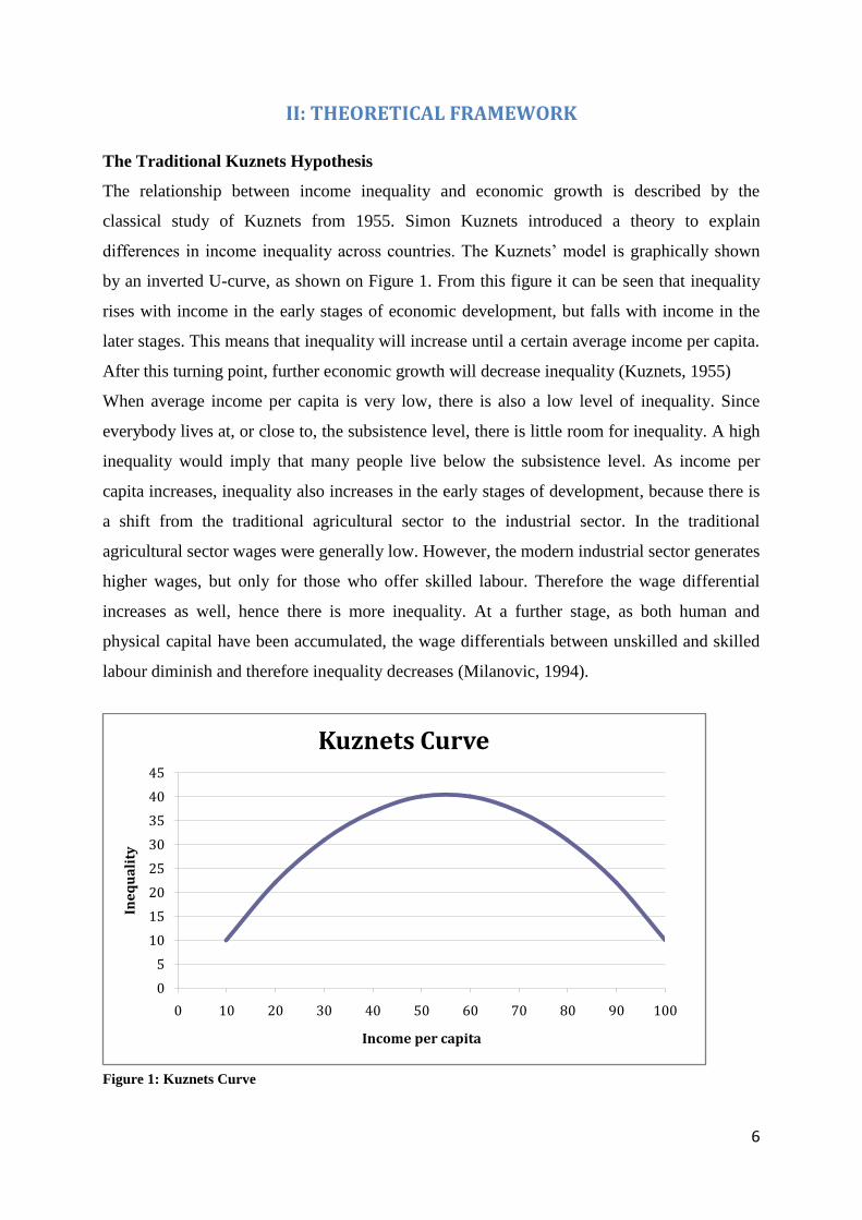
The relationship between income inequality and economic growth is described by the

classical study of Kuznets from 1955. Simon Kuznets introduced a theory to explain

differences in income inequality across countries. The Kuznets’ model is graphically shown

by an inverted U-curve, as shown on Figure 1. From this figure it can be seen that inequality

rises with income in the early stages of economic development, but falls with income in the

later stages. This means that inequality will increase until a certain average income per capita.

After this turning point, further economic growth will decrease inequality (Kuznets, 1955)

When average income per capita is very low, there is also a low level of inequality. Since

everybody lives at, or close to, the subsistence level, there is little room for inequality. A high

inequality would imply that many people live below the subsistence level. As income per

capita increases, inequality also increases in the early stages of development, because there is

a shift from the traditional agricultural sector to the industrial sector. In the traditional

agricultural sector wages were generally low. However, the modern industrial sector generates

higher wages, but only for those who offer skilled labour. Therefore the wage differential

increases as well, hence there is more inequality. At a further stage, as both human and

physical capital have been accumulated, the wage differentials between unskilled and skilled

labour diminish and therefore inequality decreases (Milanovic, 1994).

Figure 1: Kuznets Curve

0

5

10

15

20

25

30

35

40

45

0 10 20 30 40 50 60 70 80 90 100

Ine

qu

ali

ty

Income per capita

Kuznets Curve

7

Early Stages of Development

There are several mechanisms underlying the relationship between economic growth and

income inequality, as mentioned by Kuznets (1955). Although the data available was limited

in the 1950s, Kuznets managed to come up with some important implications concerning this

relationship. He suggested that in order to answer the question how income inequality

changes in the process of a country’s economic growth, we have to look at the already

developed countries. Kuznets used the size distribution of income within the United States,

England and Germany and concluded that inequality first levelled off and later declined with

an increase in economic development. However, finding a long-term steady state or even

reduction of inequality for these developed countries is quite hard. This is due to two sources

that lead to increasing inequality. The first source concerns the concentration of savings in the

upper-income brackets. Since the low-income groups have barely enough money to pay for

their daily consumptions, only the upper-income groups are able to save part of their earned

money. Therefore, it is not surprising that these groups also have the largest proportion of

income-yielding assets in their hands. The second source concerns the industrial structure of

income distribution. Income distribution is a combination of the rural and the urban

populations. According to Kuznets, it is widely known that (i) the average per capita income

of the rural population is usually lower than that of the urban and (ii) inequality in the

percentage shares within the distribution for the rural population is somewhat narrower than

in that for the urban population. This leads to the idea that a major shift from the rural to the

urban sector increases the weight of the unequal sector, triggering an increase in overall

inequality. Moreover, this idea also holds if the assumption of wider inequality in the urban

sector is relaxed, since income levels between urban and rural sectors are large due to

productivity gains in the urban sector (Moran, 2005). These two sub-theories explain the

simultaneous increase in inequality and economic growth.

Later Stages of Development

Since we now know the theories underlying the increase in income inequality corresponding

to an increase in economic growth, it is also important to know how the reversal of this trend

can be explained. Kuznets (1955) argued that: “Once the early turbulent phases of

industrialization and urbanization had passed, a variety of forces converged to bolster the

economic position of the lower-income group within the urban population.” (p. 17).

Furthermore, he stated: “The major offset to the widening of income inequality associated

with the shift from agriculture and the countryside to industry and the city must have been a

8

rise in the income share of the lower groups within the non-agricultural sector of the

population.” (Kuznets, 1955, p. 17). Due to the urbanization of a country, the size of the rural

sector diminishes and hence more of the poor agricultural workers will join the relatively rich

industrial sector. Besides this, the workers who started at the bottom of the industrial sector

were able to move up within this sector. Therefore, more people will earn the higher industrial

wage. Moreover, the relative wages in the agricultural sector increase due to the decrease in

the size of the agricultural labour force. This leads to an overall reduction in income

inequality. Thus, we can conclude that at later stages of development, the relation between

economic growth and income inequality is negative (Barro, 1999).

Kuznets’ Theory about developing countries

In the light of the research question:”Can economic growth in developing countries help to

reduce poverty and income inequality?” it is interesting to know what Kuznets’ theory says

about the reasons behind poverty and inequality in developing countries. Although the data

used by Kuznets is quite narrow and he only looked at the difference between developed and

developing countries, his findings can still help to find an answer. Kuznets particularly

looked at the data after the Second World War and only acquired such for India, Sri Lanka

and Puerto Rico. He found that these developing countries are characterized by a more

unequal income distribution compared to the sample of developed countries, namely England,

Germany and the United States. By taking a closer look at the difference between India and

the United States, he argued that the higher income inequality in India is due to the fact that

the country has no ‘middle’ class. This leads to a sharp contrast between the large proportion

of the population who have an income well below the countrywide average and the very small

proportion of the population with a very high income. The United States show a much more

gradual rise in income and the income of the small top group does not exceed the countrywide

average by a substantial amount. Due to this finding, one can argue that even the distributions

of secular income levels would be more unequal in developing countries compared to the

level in developed countries (Kuznets, 1955). This would lead to a variety of implications, of

which three are discussed below.

In the first implication, Kuznets suggests that the developing countries have a much lower

level of average income per capita. Therefore, a below-average income level in these

countries is accompanied by much greater material and psychological misery than in

developed countries. Moreover, the concentration of savings and assets is more pronounced in

9

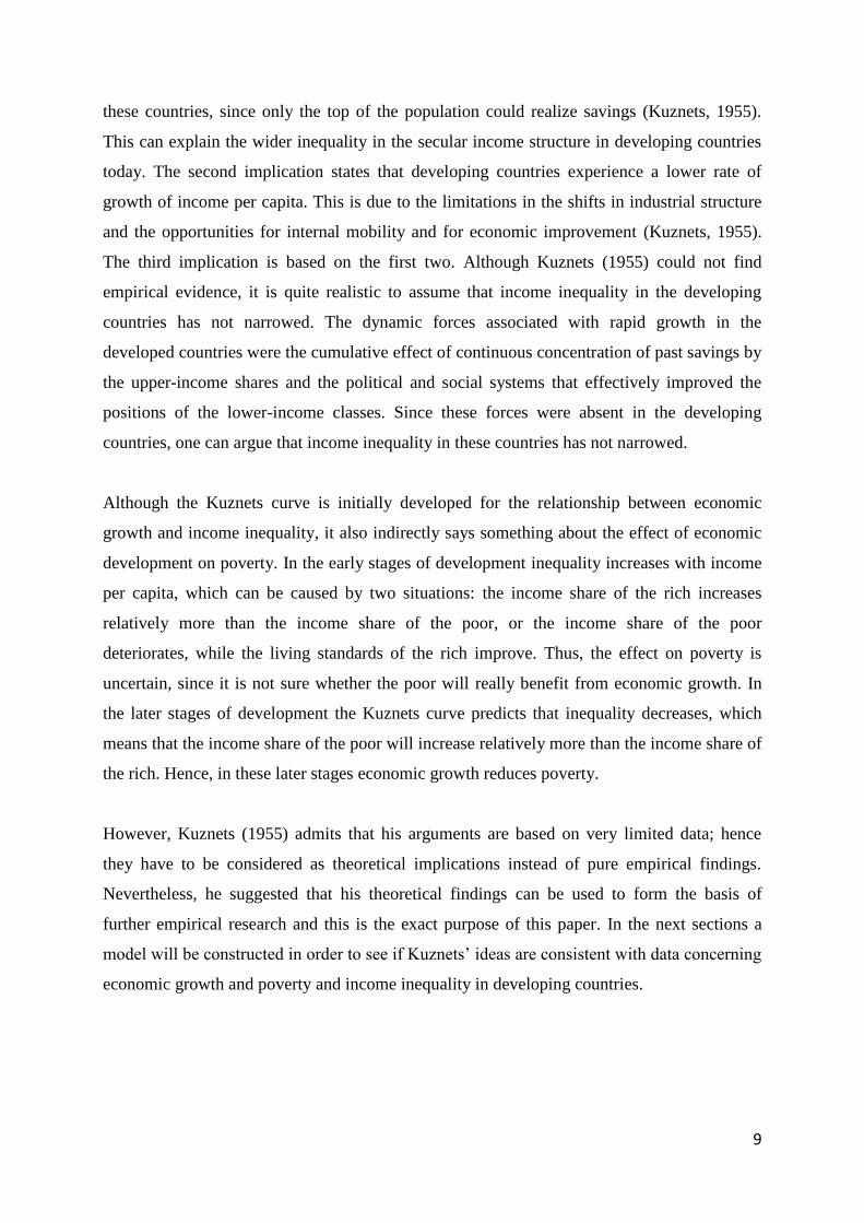
these countries, since only the top of the population could realize savings (Kuznets, 1955).

This can explain the wider inequality in the secular income structure in developing countries

today. The second implication states that developing countries experience a lower rate of

growth of income per capita. This is due to the limitations in the shifts in industrial structure

and the opportunities for internal mobility and for economic improvement (Kuznets, 1955).

The third implication is based on the first two. Although Kuznets (1955) could not find

empirical evidence, it is quite realistic to assume that income inequality in the developing

countries has not narrowed. The dynamic forces associated with rapid growth in the

developed countries were the cumulative effect of continuous concentration of past savings by

the upper-income shares and the political and social systems that effectively improved the

positions of the lower-income classes. Since these forces were absent in the developing

countries, one can argue that income inequality in these countries has not narrowed.

Although the Kuznets curve is initially developed for the relationship between economic

growth and income inequality, it also indirectly says something about the effect of economic

development on poverty. In the early stages of development inequality increases with income

per capita, which can be caused by two situations: the income share of the rich increases

relatively more than the income share of the poor, or the income share of the poor

deteriorates, while the living standards of the rich improve. Thus, the effect on poverty is

uncertain, since it is not sure whether the poor will really benefit from economic growth. In

the later stages of development the Kuznets curve predicts that inequality decreases, which

means that the income share of the poor will increase relatively more than the income share of

the rich. Hence, in these later stages economic growth reduces poverty.

However, Kuznets (1955) admits that his arguments are based on very limited data; hence

they have to be considered as theoretical implications instead of pure empirical findings.

Nevertheless, he suggested that his theoretical findings can be used to form the basis of

further empirical research and this is the exact purpose of this paper. In the next sections a

model will be constructed in order to see if Kuznets’ ideas are consistent with data concerning

economic growth and poverty and income inequality in developing countries.

10

III: LITERATURE REVIEW

As described in chapter 2, the relationship between economic growth and income inequality is

graphically shown by an inverted U-curve: inequality rises with income in the early stages of

economic development, but falls with income in the later stages, since the poorest people will

also benefit and there will be an improvement of the economy as a whole (Kuznets, 1955).

However, whether the relationship between growth and inequality is indeed an inverted U-

curve still remains an empirical issue. There have been many studies analyzing the

interdependence between economic growth and poverty and income inequality in developed

as well as developing countries. Still, the empirical literature on this relationship does not

provide consistent results. In section 3.1 there will be a review of the literature concerning the

impact of economic growth on income inequality. Subsequently, in section 3.2 there will be a

discussion of previous studies on the relationship between economic development and

poverty.

3.1 Growth and income inequality

One of the empirical investigations concerning the relationship between growth and inequality

was performed by Ravallion (1995). He used cross-country data for 36 developing countries

in the 1980s, which represented more than 70 percent of the population in the developing

world. The results show no empirical evidence for a systematic interaction between the Gini

coefficient and the mean income. Even when controlling for country-level fixed effects,

Ravaillon (1995) rejects the Kuznets hypothesis. The data indicate that growth does not

increase or decrease inequality.

Deininger and Squire (1998) examined the relation between long-term growth and inequality

using cross-country data on income and asset distribution. In this paper, the Kuznets curve is

empirically investigated using data for developed and developing countries over the world.

The estimation results do not provide enough empirical support for a cross-country Kuznets

curve. Even when testing the Kuznets curve for individual countries, the results indicate that

changes in per capita income are not significantly related to changes in inequality in most of

the analyzed countries. Many countries with a low per-capita income initially, experienced a

high economic growth but no increase in inequality. On the contrary, for some countries the

results did show evidence for the Kuznets hypothesis. Nevertheless, the results rejected the

Kuznets curve almost as often as confirming it (Deininger and Squire, 1998). Deininger and

11

Squire (1998) even conclude that the Kuznets hypothesis is not relevant for developing

countries.

Li and Zou (1998) empirically investigated the Kuznets curve and based their statistical

analysis on the expanded dataset on income distribution constructed by Deininger and Squire

in 1996. The authors created a theoretical model that indicates a positive relation between

economic growth rate and income inequality, assuming that income inequality may give rise

to economic growth if the model takes account of public consumption. This relation is

empirically analyzed by regressing GDP growth rate on the Gini coefficient (as a measure of

inequality) and other control variables like population growth rate and trade openness. Li and

Zou (1998) performed panel estimation, using data from 46 developed and developing

countries over the period 1947-1994. The estimated coefficients showed indeed a positive

interaction between economic growth and inequality, which was significant in many cases (Li

and Zou, 1998).

Barro (2000) used data for a broad panel of 84 countries to examine the interaction between

income inequality and rates of growth and investment. To extend this framework, Barro

(2000) used some determinants for economic growth. Furthermore, the Gini coefficient is

used as a measure of inequality considering 10-year values around 1960, 1970, 1980 and

1990. The estimation results show cross-sectional variations among countries, but also

differences over time within countries. The available evidence indicates a negative

relationship between income inequality and economic growth for countries with a low GDP

per capita on the one hand and a positive interaction for countries with a high GDP per capita

on the other hand. In low-income regions, inequality seems to decelerate growth, while in

high-income regions inequality seems to stimulate economic expansion. Furthermore, the

estimation results indicate that growth falls with inequality when the income per capita is

lower than $2000 and increases with inequality when the income per capita is larger than

$2000 (Barro, 2000). Hence, this result implies a U-curve instead of an inverted U-curve as

assumed by the Kuznets hypothesis. Since the curve does not fit the data, Barro (2000)

concludes that the Kuznets relation does not empirically explain the differences in inequality

over time or across countries.

Forbes (2000) argued that previous studies analyzing the relationship between growth and

income inequality were limited by data availability concerning cross-country statistics for

12

inequality. Limited data availability can lead to measurement error and omitted-variable bias,

since the time-series dimension was not large enough to perform a panel study. Forbes (2000)

re-estimated the interaction between growth and inequality, challenging the belief that there is

a negative interaction. To empirically analyze this relationship, Forbes (2000) used an

improved and more consistent data set on income inequality to avoid measurement error. The

data set included observations for 45 (developed and developing) countries over the world for

the period 1966 until 1995. The Gini coefficient was used as a measure of inequality, which

was taken from the latest available data. Forbes (2000) used the panel technique as an

estimation method, arguing that this technique provides an accurate and clearer estimation of

the correlation between changes in growth rate and changes in inequality. Another reason for

using panel estimation was to account for omitted-variable bias, since it controls for country-

specific effects. The estimation results imply that there is a significant positive relationship

between economic growth and the level of income inequality within individual countries. This

relation holds only for the short and medium term, since Forbes (2000) used five-year panels

to estimate the coefficients. Although the results are robust across samples and model

specification, the relationship may not hold for very low-income regions, because of limited

data availability for poor countries. Furthermore, the positive interaction between growth and

inequality may not hold in the long run, considering periods longer than ten years (Forbes,

2000).

Banerjee and Duflo (2003) investigated the interaction between growth and inequality in

cross-country data. To empirically examine this relationship, Banerjee and Duflo (2003) used

the data set on income inequality constructed by Deininger and Squire in 1996. This data set

has more reliable and improved measures of inequality (for instance Gini coefficients and

quintile shares of income), which should lead to better results compared to other data sets.

Furthermore, the data set contains data for a large number of countries, including developed

and developing countries. The analysis by Banerjee and Duflo (2003) is based on a time

period of 5 years and 10 years. The estimation results confirm the Kuznets hypothesis: the

data shows an inverted U-shaped relationship between growth and inequality. Changes in

inequality seem to be associated with changes in economic growth.

Perotti (1996) examined the relation between democratic institutions, income distribution and

economic growth by analyzing the channels through which income distribution has an impact

on growth. The dataset used includes income quintile shares for 67 countries over the world,

13

which are used as a measure of inequality. The results indicate a negative impact of inequality

on growth. This conclusion is based on three main channels, namely, fertility rate,

sociopolitical instability and investment in education. Perotti (1996) argues that more equal

societies have more investments in human capital and lower fertility rates, which leads to

larger economic growth. On the contrary, more unequal societies are often politically and

socially unstable, leading to lower investments in education, which have a negative impact on

economic growth.

These empirical studies use different data and estimation methods, which lead to mixed

results and an unclear representation of the relationship between economic growth and

inequality. Furthermore, most of the previous studies focus on the impact of inequality on

economic development. To contribute to the existing literature, this paper analyzes the reverse

relationship using the most recent data.

3.2 Growth and poverty

It seems obvious that economic growth should reduce poverty, but the persistent problem of

poverty in developing countries has led many to question the effectiveness of economic

growth to increase the living standards of the poor. Ravaillon (1995) examined the

relationship between economic growth and poverty using data for developing countries in the

1980s. The results indicate a negative interaction between average living standards and the

levels of poverty: a three percent growth in consumption per capita leads to more than six

percent reduction in the people living below the poverty line of $1 per day. Although

economic development seems to benefit the poor, there are still differences in poverty

reduction between countries at a given growth rate (Ravaillon, 1995).

Roemer and Gugerty (1997) analyzed the interdependence between economic development

and poverty using data for 26 developing countries. They used the growth of income of the

poorest 20 percent and the poorest 40 percent of the population as poverty indicators and

regressed these calculations against the growth of GDP per capita. The estimation results

indicate that economic growth benefits the poor. For the poorest 40 percent of the population,

the rate of GDP growth has a one-to-one relationship with the average incomes. For example,

when GDP per capita grows with ten percent, the average incomes of the 40 percent poorest

of the population will also rise with ten percent. For the 20 percent poorest of the population

this relationship is also positive, but weaker, with an elasticity of 0.921. Hence, these results

14

show that economic growth reduces poverty (Roemer & Gugerty, 1997). Furthermore,

Roemer and Gugerty (1997) also show that macroeconomic policies and trade openness can

be useful in alleviating poverty, since good policies lead to a faster GDP growth.

Another estimation of the relationship between growth and poverty was performed by Dollar

and Kraay (2002), who examined how incomes of the poor vary with overall incomes. They

used a data set covering observations for 92 countries over the period 1950-1999. Poverty was

measured as the income share of the poorest 20 percent of the population. The results show

that average incomes of the poorest 20 percent increase or decrease at almost the same rate as

average incomes of the whole population. The reason behind this result is that the share of

income of the poorest group does not vary systematically with the average income of the

whole population. The corresponding interaction seems to hold across countries and income

levels and even during crises. Furthermore, the results show that macroeconomic policies like

trade openness benefit the poor, since their incomes increase (Dollar & Kraay, 2002). Dollar

and Kraay (2002) conclude that economic growth benefits the poor to the same extent as other

groups in the society and growth-enhancing policies can be useful for alleviating poverty.

Although these studies imply that economic growth benefits the poor, there have not been

many studies analyzing the relationship between growth and poverty. Furthermore, the studies

use datasets with time periods earlier than 2000. This paper contributes to the literature by

using the most recent data to analyze the relationship between economic development and

poverty.

15

IV: DATA AND METHODOLOGY

In this chapter there will be a description of the data and the techniques used to assess the

relationship between economic development and poverty and inequality. In addition, there

will also be an explanation of the methods used to analyze the relationship between economic

development and the drivers behind economic growth. First the selection of the data will be

discussed. Afterwards, there will be a description of the estimation technique and the model

specification.

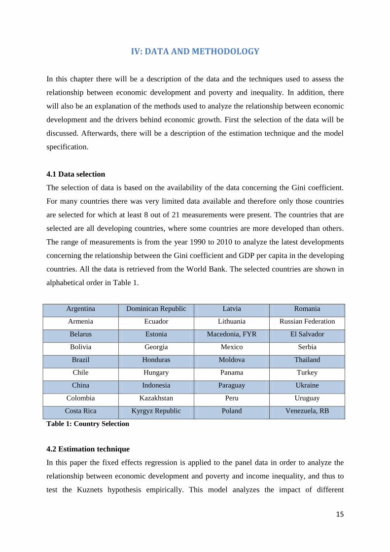
4.1 Data selection

The selection of data is based on the availability of the data concerning the Gini coefficient.

For many countries there was very limited data available and therefore only those countries

are selected for which at least 8 out of 21 measurements were present. The countries that are

selected are all developing countries, where some countries are more developed than others.

The range of measurements is from the year 1990 to 2010 to analyze the latest developments

concerning the relationship between the Gini coefficient and GDP per capita in the developing

countries. All the data is retrieved from the World Bank. The selected countries are shown in

alphabetical order in Table 1.

Argentina Dominican Republic Latvia Romania

Armenia Ecuador Lithuania Russian Federation

Belarus Estonia Macedonia, FYR El Salvador

Bolivia Georgia Mexico Serbia

Brazil Honduras Moldova Thailand

Chile Hungary Panama Turkey

China Indonesia Paraguay Ukraine

Colombia Kazakhstan Peru Uruguay

Costa Rica Kyrgyz Republic Poland Venezuela, RB

Table 1: Country Selection

4.2 Estimation technique

In this paper the fixed effects regression is applied to the panel data in order to analyze the

relationship between economic development and poverty and income inequality, and thus to

test the Kuznets hypothesis empirically. This model analyzes the impact of different

16

explanatory variables that vary over time. Furthermore, the fixed effects model also controls

for factors within the country that may bias the dependent or independent variables, thus it

controls for correlation between the error term and these variables. In addition, this model

eliminates the effect of time-invariant characteristics from the explanatory variables and

leaves behind the net effect of these variables. Thus, this fixed effects regression allows us to

take into account the different effects that are fixed within each country, as they may be

heterogeneous. Below there will be a description of the dependent and independent variables

used in the regression analysis.

Gini coefficient

There are several ways of computing income inequality, for example by using the Gini-index,

Theil index or Decile Dispersion index (The World Bank, 2014). Each method has both

advantages and disadvantages. The biggest disadvantage of the Theil index is that the values

are not always comparable across different units (for example countries or years). Since the

chosen data consists of different countries as well as different years, the Theil index is not

preferable. The Decile Dispersion Index is also not suitable for this research, because it is

very vulnerable to extreme values. Since it is difficult to exclude the occurrence of extreme

values beforehand, this method is also not the preferred one. The only option left is the Gini

coefficient. The disadvantage of the Gini coefficient is that the total Gini of the total

population is not equal to the sum of the Gini indices for its subgroups. However, this would

not cause any problem, since this research is based on comparing the total population and not

the subgroups (The World Bank, 2014). Therefore, the Gini-coefficient is used to estimate the

degree of income inequality. The Gini coefficient is usually estimated according to the

following formula: G = 1 - Σ (Pi * ( Qi + Qi-1 )). In this formula, the variable Pi stands for the

population share of income group i and Qi stands for the cumulative income share up to

income group i. The Gini index measures the difference between the actual distribution of

income or consumption expenditure within an economy and a perfectly equal distribution.

The index ranges from 0 to 100, where the value 0 refers to perfect equality, while 100

indicates a degree of perfect inequality (The World Bank, 2014).

Income share held by lowest 20 percent

In this paper, the income share held by the lowest 20 percent of the population is used as a

poverty indicator to analyze the relationship between economic growth and poverty over time.

This percentage share of income is the share that accrues to subgroups of population indicated

17

by deciles or quintiles (The World Bank, 2014). This variable is chosen, since many previous

studies have used income shares of the poor as a poverty indicator.

Real GDP per capita

Real GDP per capita is representing a country’s wealth and is key in testing the Kuznets

hypothesis. Therefore it is used as a measure for economic development. In this research, real

GDP per capita is represented by the gross domestic product converted to international dollars

using purchasing power parity rates (PPP). The PPP conversion factor for GDP is defined as

the number of units of a country’s currency required to buy the same amounts of goods and

services in the domestic market as U.S. dollar would buy in the United States. In addition,

GDP at purchaser’s prices also refers to the sum of gross value added by all resident

producers in the economy plus any product taxes and minus any subsidies not included in the

value of the products. Deductions for depreciation of fabricated assets, depletion and

degradation of natural resources are also excluded (The World Bank, 2014).

The following control variables that may influence the relationship between economic growth

and poverty and inequality are selected and added to the regression:

Education

Education is a factor that very likely will affect economic growth and income inequality.

According to theory, the impact of education on income inequality is non-linear, following the

same pattern of the Kuznets curve. There are two effects that can have different impacts on

income inequality. The first one is the ‘composition’ effect: when the relative size of the

group with more education increases, this initially raises income inequality but eventually

lowers it. The reason is that as the group of educated people grows, education is not a scarce

factor anymore. The second one is the ‘wage compression’ effect: this effect decreases the

wage rate for educated people as the relative supply of educated workers increases, thereby

lowering income inequality (Gregorio & Lee, 1999).

The relationship between education and poverty can be explained through the labour market:

the higher the level of education, the larger the productivity and the larger the probability of

finding a job and thus the higher the earnings (Berg, 2008). This result implies that education

improves the living standards of the poor and is therefore necessary for poverty reduction.

Education can be measured by several indicators, for example public expenditure on

education, school enrollment, literacy rate, primary completion rate and progression to

secondary school. Although public spending on education is a good indicator for education

18

investments, it is not useful for this research, because public education investments in each

year will usually yield economic results after a few years. Hence, with this measure of

education one cannot estimate the direct relationship between education and economic

development or inequality in a given year. Based on data availability, the primary completion

rate is used as an indicator for education. The primary completion ratio includes the total

number of new entrants in the last grade of primary school, irrespective of age, expressed as a

percentage of the total population of the theoretical entrance age to this last grade. The rate

can exceed 100 percent because of over-aged and under-aged children who enter primary

school early or late and children who repeat grades (The World Bank, 2014). The primary

completion rate can influence inequality, poverty or economic development earlier compared

to public spending on education. Furthermore, it is also reasonable to assume that a part of the

public spending on education invested years before is included in this rate of primary

completion. The reason for this is that public spending on education does not only include

investments in educational institutions, but also subsidies for students or households, which

could have helped people to achieve a primary degree after a few years.

FDI Inflows

Foreign Direct Investment is a long-term investment reflecting a lasting management interest

in and control by a resident entity in one economy of an enterprise operating in a different

economy. ‘Control’ refers to acquiring at least 10 percent of the outstanding stocks of the

company. FDI includes the sum of reinvestment of earnings, equity capital and other long-

term and short-term capital (The World Bank, 2014). In this paper, the net inflows of FDI in a

country as a percentage of GDP are used as a control variable. The net inflows refer to new

investments minus disinvestments. A previous empirical study shows that the impact of

foreign direct investments on income inequality is positive, but it does depend on the level of

absorptive capacity in the host country (Wu & Hsu, 2012). Absorptive capacity defines the

ability of a firm to recognize the economic potential of newly introduced information,

assimilate it, and apply it commercially (Cohen & Levinthal, 1990). It is shown that FDI has

little impact on income inequality when the host country has high absorptive capacity and a

large impact when the level of absorptive capacity is low (Wu & Hsu, 2012). Furthermore,

Klein et al (2001) argue that FDI is a key factor for achieving economic growth and indirectly

reducing poverty.

19

Credit Market

To account for capital market imperfections, the lending interest is also used as a control

variable. It refers to the interest rate provided by banks for short- and medium-run loans to the

private sector. The rate usually depends on the creditworthiness of borrowers and the aims of

financing (The World Bank, 2014). The lending interest rate can affect income inequality,

since it differs between countries due to different terms and conditions and different risk

premiums. The interest rate is expected to be higher in countries which are less developed,

because the risk for the lender is higher as a result of the widespread lack of collateral. The

higher the interest rate, the fewer the people who have access to credit. Therefore, if a small

proportion of the population has access to credit, this might increase the income inequality

within a country. Thus, a positive relation between the lending interest rate and income

inequality is expected. In addition, a lower interest rate increases the access to credit and can

be an important factor in reducing poverty.

Unemployment rate

The rate of unemployment measures the share of the labour force which is not currently

working, but is able to work and actively seeking employment (The World Bank, 2014).

Although definitions of unemployment may differ across countries, it is assumed to be a good

approximation of the share of the population which is not employed at a given time. A study

conducted by Aaberge et al. (2000) has established that a low level of unemployment is

associated with a more equal income distribution and a lower level of poverty. Therefore, it

can be assumed that a high level of unemployment will lead to a higher level of income

inequality and more poverty.

Inflation

Inflation is included as a control variable, because it can be correlated with poverty and

income inequality. In order to show the rate of price change in the economy as a whole,

inflation in this model is measured with the GDP deflator. This means that the annual growth

rate of the GDP implicit deflator is used, and it is calculated as the ratio of GDP in current

local currency to GDP in constant local currency (The World Bank, 2014). The research by

Albanesi (2006) shows that inflation and income inequality are positively related. Cardoso

(1992) argues that during inflation the rise in wages is more slowly than the rise in prices,

which can increase poverty.

20

Trade Openness

Trade Openness’ in included as a control variable because it also might be correlated with

income inequality. According to the Stolper-Samuelson theorem, trade liberalization will shift

income toward a country’s abundant factor (Davis, 1996). Developed countries are overall

capital abundant. This is primarily the sector in which high-educated people work. As the

degree of exports and thus trade openness increases, we expect the income to shift to the high-

educated people. Conversely, developing countries are overall labour abundant. This is

primarily the sector in which low-educated people work. As the degree of exports increases,

we expect the income to shift to the low-educated people. Hence, one can conclude that

exports are positively correlated to income inequality considering developed countries, ceteris

paribus. On the contrary, exports are negatively correlated to income inequality and poverty

considering developing countries, ceteris paribus. Furthermore, mainly the rich people in

developing countries are able to import goods and services from abroad, especially in the case

of luxury goods. If the goods contribute to future productivity and improve the living

standards of the rich, this could increase the income inequality within the country and thus a

positive relationship is expected concerning imports and inequality.

Both exports and imports of goods and services as a percentage of GDP are representing the

degree of trade openness of a country. The higher the exports and imports of a country, the

more a country is trading with other countries, and hence the more open to trade the country

is. Exports of goods and services as a percentage of GDP: a measure for the value of all

goods and other market services provided by the country to other all countries in the world

(The World Bank, 2014). Imports of goods and services as a percentage of GDP: a measure

for the value of all goods and other market services provided by the world to the country of

interest (The World Bank, 2014).

4.3 Model specification

To get a clear overview of the relationship between economic growth and poverty and

inequality, various regressions are used. All regressions are based on country and time fixed

effects. The regressions for the analysis concerning economic growth and inequality, where

the Gini coefficient is the dependent variable, are as follows:

Regression 1: Basic Regressions

𝐺𝑖𝑛𝑖𝑖𝑡 = β0 + β1 ∗ GDPit + Ɛit

21

𝐺𝑖𝑛𝑖𝑖𝑡 = β0 + β1 ∗ GDPit + β2 ∗ GDPit2 + Ɛit

Regression 2: Regression including all control variables

𝐺𝑖𝑛𝑖𝑖𝑡 = β0 + β1 ∗ GDPit + β2 ∗ GDPit2 + β3 ∗ EDUC𝑖𝑡 + β4 ∗ FDI𝑖𝑡 + β5 ∗ CM𝑖𝑡 + β6 ∗ UNEM𝑖𝑡

+ β7 ∗ INF𝑖𝑡 + β8 ∗ EXP𝑖𝑡 + β9 ∗ IMP𝑖𝑡 + Ɛit

The regressions to analyze the impact of economic growth on poverty are listed below. In

these regressions, the income share held by the lowest 20 percent of the population (ISL) is

the dependent variable.

Regression 1: Basic Regressions

𝐼𝑆𝐿𝑖𝑡 = β0 + β1 ∗ GDPit + Ɛit

𝐼𝑆𝐿𝑖𝑡 = β0 + β1 ∗ GDPit + β2 ∗ GDPit2 + Ɛit

Regression 2: Regression including all control variables

𝐼𝑆𝐿𝑖𝑡 = β0 + β1 ∗ GDPit + β2 ∗ GDPit2 + β3 ∗ EDUC𝑖𝑡 + β4 ∗ FDI𝑖𝑡 + β5 ∗ CM𝑖𝑡 + β6 ∗ UNEM𝑖𝑡

+ β7 ∗ INF𝑖𝑡 + β8 ∗ EXP𝑖𝑡 + β9 ∗ IMP𝑖𝑡 + Ɛit

The reason for this stepwise estimation of the relationship is to prove the existence of a robust

effect of real GDP per capita on income inequality and poverty. In these regressions, GDP

refers to the real GDP per capita in US dollars and EDUC denotes the primary completion

rate. FDI stands for the inflows of foreign direct investment, while CM denotes the lending

interest rate on the credit market. The variable UNEM refers to the share of the labour force

which is not currently working, but is able to work and actively seeking employment. INF

refers to the inflation rate and IMP and EXP are the imports and exports as a percentage of

GDP. Finally, Ɛ is the stochastic error term, the subscript t denotes the year with t = 1

referring to the year 1990 and the subscript i refers to the different countries.

In order to have a first impression of the relationship between economic development and

poverty and income inequality, two scatter plots are made for the complete sample of

developing countries.

22

20

30

40

50

60

70

0 5,000 10,000 15,000 20,000 25,000

Real GDP per capita

GIN

I

0

2

4

6

8

10

12

0 5,000 10,000 15,000 20,000 25,000

GDP per capita

Inco

me

sh

are

lo

we

st

20

%

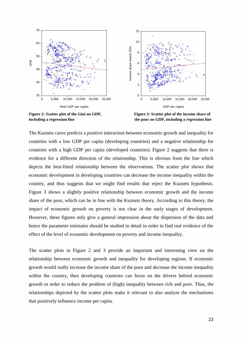
Figure 2: Scatter plot of the Gini on GDP, Figure 3: Scatter plot of the income share of

including a regression line the poor on GDP, including a regression line

The Kuznets curve predicts a positive interaction between economic growth and inequality for

countries with a low GDP per capita (developing countries) and a negative relationship for

countries with a high GDP per capita (developed countries). Figure 2 suggests that there is

evidence for a different direction of the relationship. This is obvious from the line which

depicts the best-fitted relationship between the observations. The scatter plot shows that

economic development in developing countries can decrease the income inequality within the

country, and thus suggests that we might find results that reject the Kuznets hypothesis.

Figure 3 shows a slightly positive relationship between economic growth and the income

share of the poor, which can be in line with the Kuznets theory. According to this theory, the

impact of economic growth on poverty is not clear in the early stages of development.

However, these figures only give a general impression about the dispersion of the data and

hence the parameter estimates should be studied in detail in order to find real evidence of the

effect of the level of economic development on poverty and income inequality.

The scatter plots in Figure 2 and 3 provide an important and interesting view on the

relationship between economic growth and inequality for developing regions. If economic

growth would really increase the income share of the poor and decrease the income inequality

within the country, then developing countries can focus on the drivers behind economic

growth in order to reduce the problem of (high) inequality between rich and poor. Thus, the

relationships depicted by the scatter plots make it relevant to also analyze the mechanisms

that positively influence income per capita.

23

Economic growth or GDP growth can be achieved through several mechanisms. In this paper

there will an implicit focus on two important drivers behind economic growth, which are

education and foreign direct investment (FDI) inflows.

In general, schooling improves job prospects for the poor and makes it possible to avoid

living in poverty. Hanushek and Wößmann (2007) argue that education investments have

powerful effects on economic growth. The distribution of skills in a nation seems to be

closely related to the distribution of income. Better cognitive skills increase the individual

earnings and result in stronger economic performance of countries. Even when controlling

for other factors that are also important for economic development like open markets and

established property rights, the quality of education seems to have a significant impact on the

economic earnings of a nation (Hanushek and Wößmann, 2007). In addition, the cross-

country regressions by Krueger and Lindahl (2000) also show a positive relationship between

education investments and economic development. Thus, based on these empirical results one

can assume that a more skilled population contributes to economic growth.

There have also been a few studies analyzing the relationship between foreign direct

investments and economic development. Klein et al (2001) argue that FDI inflows have a

positive impact on economic growth and poverty reduction. These foreign investments lead to

a rapid and efficient transfer of improved techniques and methods, which increase the

economic earnings. Alfaro, Chanda, Kalemli-Ozcan and Sayek (2004) analyzed the

interactions between FDI, financial markets and economic growth. The empirical results,

which are based on cross-country data between 1975 and 1995, indicate that foreign

investments have a positive effect on the economic development of a country. Furthermore,

the authors also argue that good financial markets are necessary for these positive effects to be

realized in a beneficial way (Alfaro et al, 2004).

In order to control for other factors, a few variables that may influence the relationship

between economic growth and the mechanisms are added to the regression.

The empirical study by Fischer (1993) shows a negative interaction between economic

development and inflation. Using cross-sectional and panel regressions, Fischer (1993) argues

that a high rate of inflation reduces investments and the rate of productivity growth and

therefore reduces economic growth. The empirical results are in line with the view that a

stable macroeconomic environment, meaning a reasonably low rate of inflation, is necessary

for sustained economic growth. Credit market imperfections can also have a powerful impact

24

on economic growth. As mentioned before, the lending interest rate is expected to be higher in

developing countries, because the risk for the lender is higher as a result of the widespread

lack of collateral. A high interest rate decreases the access to credit and investments, which

can be an impediment to economic growth. Therefore, a negative relationship is expected

between the lending interest rate and economic growth.

Another variable that could influence economic development is trade openness. Harrison

(1996) analyzed the impact of different openness measures on economic growth and found a

positive relationship: a greater openness seems to be associated with a higher growth.

Furthermore, more openness measures seem to positively influence economic growth when

using panel data compared to cross-section data.

To analyze the impact and significance of education and FDI on real GDP per capita, the

following regressions are used:

Regression 1: Basic regression

𝐺𝐷𝑃𝑖𝑡 = β0 + β1 ∗ CMit + β2 ∗ INF𝑖𝑡 + β4 ∗ EXP𝑖𝑡 + β5 ∗ IMP𝑖𝑡 + Ɛit

Regression 2: Regression including the variable education

𝐺𝐷𝑃𝑖𝑡 = β0 + β1 ∗ EDUCit + β2 ∗ CM𝑖𝑡 + β3 ∗ INF𝑖𝑡 + β4 ∗ EXP𝑖𝑡 + β5 ∗ IMP𝑖𝑡 + Ɛit

Regression 3: Regression including the variable FDI inflows

𝐺𝐷𝑃𝑖𝑡 = β0 + β1 ∗ FDIit + β2 ∗ CM𝑖𝑡 + β3 ∗ INF𝑖𝑡 + β4 ∗ EXP𝑖𝑡 + β5 ∗ IMP𝑖𝑡 + Ɛit

The first regression includes only control variables. Afterwards, the variables education and

FDI investments are added separately to this basic regression in order to check the

significance and explanatory power of these mechanisms, given the control variables that may

influence the corresponding relationship. The measure for education is the primary

completion rate and FDI refers to the FDI inflows in absolute numbers.

These regressions are performed for each country to analyze the impact of these drivers in

different developing countries. Subsequently, the total sample of developing countries will be

divided into two groups based on the significance of the drivers and this will be done for each

driver separately. Thus, two different groups of countries will be analyzed, where the first

group consists of developing countries where education has a significant positive impact on

25

economic development and the second group contains countries which show a significant

positive effect of FDI inflows on real income per capita. The reason for this stepwise

estimation is to analyze whether there is a different relationship between economic

development and poverty and inequality when we only look at countries where these drivers

of economic growth show a positive significant impact. The regressions performed for this

analysis can be seen below. These regressions will be performed for each group of countries.

𝐺𝑖𝑛𝑖𝑖𝑡 = β0 + β1 ∗ GDPit + β2 ∗ GDPit2 + β3 ∗ CM𝑖𝑡 + β4 ∗ UNEM𝑖𝑡 + β5 ∗ INF𝑖𝑡 + β6 ∗ EXP𝑖𝑡 + β7

∗ IMP𝑖𝑡 + Ɛit

𝐼𝑆𝐿𝑖𝑡 = β0 + β1 ∗ GDPit + β2 ∗ GDPit2 + β3 ∗ CM𝑖𝑡 + β4 ∗ UNEM𝑖𝑡 + β5 ∗ INF𝑖𝑡 + β6 ∗ EXP𝑖𝑡 + β7

∗ IMP𝑖𝑡 + Ɛit

26

V: RESULTS

In this chapter there will be a detailed discussion of the parameter estimates and other

regression results to judge the effect of the level of economic development on income

inequality and poverty, and thus to empirically test the Kuznets hypothesis. First of all, the

results concerning the relationship between real GDP per capita and the Gini coefficient will

be reviewed. Next to that, there will be a discussion of the estimation results related to the

effect of economic growth on the income share of the lowest 20 percent of the population. In

the last section, the total sample of developing countries will be divided twice into two groups

of countries, where the division will be based on the significance of education and FDI

inflows for economic development. The parameter estimates of these last regressions will be

analyzed to see whether there is a different interaction between economic growth and poverty

and inequality among the smaller sample of developing countries.

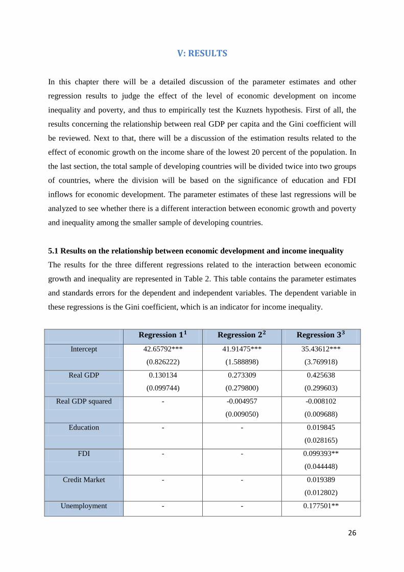
5.1 Results on the relationship between economic development and income inequality

The results for the three different regressions related to the interaction between economic

growth and inequality are represented in Table 2. This table contains the parameter estimates

and standards errors for the dependent and independent variables. The dependent variable in

these regressions is the Gini coefficient, which is an indicator for income inequality.

Regression 𝟏𝟏 Regression 𝟐𝟐 Regression 𝟑𝟑

Intercept 42.65792***

(0.826222)

41.91475***

(1.588898)

35.43612***

(3.769918)

Real GDP 0.130134

(0.099744)

0.273309

(0.279800)

0.425638

(0.299603)

Real GDP squared - -0.004957

(0.009050)

-0.008102

(0.009688)

Education - - 0.019845

(0.028165)

FDI - - 0.099393**

(0.044448)

Credit Market - - 0.019389

(0.012802)

Unemployment - - 0.177501**

27

(0.082611)

Inflation - - -0.002840

(0.002475)

Exports - - -0.062445*

(0.033493)

Imports - - 0.068525**

(0.032748)

R-squared 0.923929 0.923988 0.963032

Table 2: Parameter estimates for complete sample regression related to inequality

Robust standard errors are in parentheses. ***, ** and * indicate significance at the 1%, 5% and 10% level

respectively.

¹: Regression 1 refers to the basic regression, which only includes the variable ‘real GDP per capita’.

²: Regression 2 extends the basic regression by adding ‘real GDP per capita squared’.

³: Regression 3 extends the second regression by adding control variables.

The results reported in Table 2 demonstrate that the level of income has a positive effect on

income inequality. The parameter estimate for real GDP remains positive and even increases

when control variables are added to the regression. Thus, the estimation results indicate that

an increase in the level of real GDP per capita will result in a higher value of the Gini

coefficient. In other words, a developing country which enjoys a higher level of income per

capita will also have a higher level of inequality. This outcome contradicts the output on the

scatter plot in Figure 2, which shows a negative relationship between economic development

and income inequality. The variable GDP-squared measures the non-linear relationship

between income and inequality. This term is added to the regression analysis to have a robust

estimate. Its coefficient is negative, which implies a concave relationship between the

corresponding variables, confirming the inverted U-curve. After adding the control variables,

the parameter estimate increases in absolute values and keeps its sign. These results seem to

be in line with the Kuznets hypothesis, since Kuznets (1955) argued that countries with a low

GDP per capita (developing countries) will experience an increase in inequality during their

economic growth. However, the coefficients for real GDP and real GDP squared are not

significant in all regressions and thus the level of income has no explanatory power for the

level of inequality. Hence, we cannot confirm the Kuznets hypothesis.

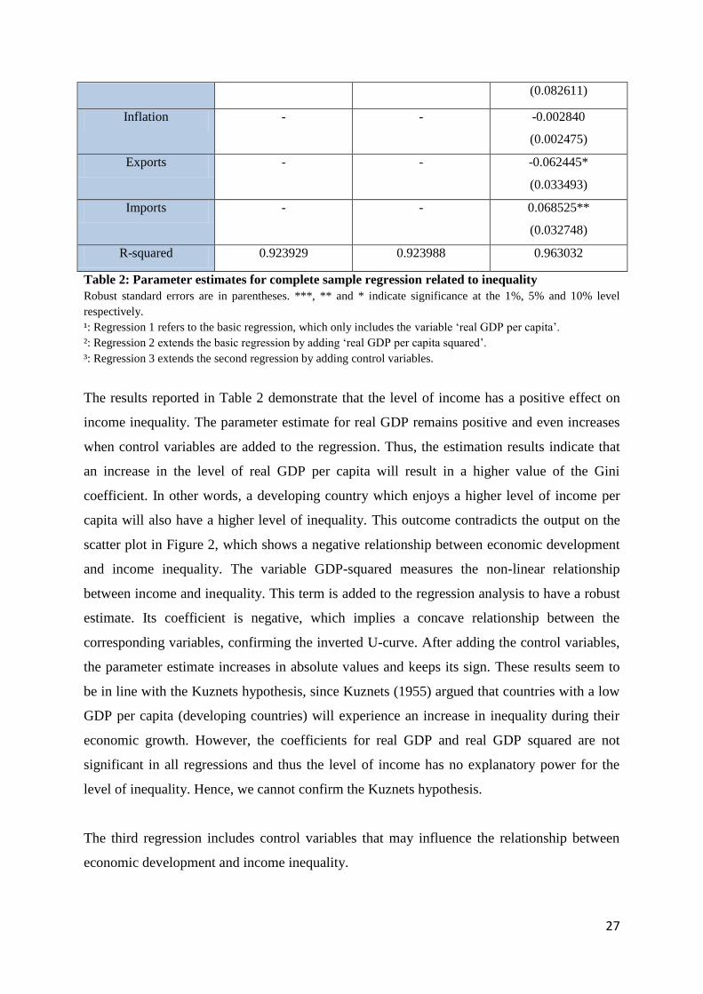
The third regression includes control variables that may influence the relationship between

economic development and income inequality.

28

The variable education has a positive sign, indicating that a higher primary completion rate

over the total population will lead to a higher level of income inequality within the country.

One would assume that having education, in this case a primary degree, would improve the

living standards of people. The estimated result contradicts the long-run impact of the

‘composition effect’ and the ‘wage compression’ effect, which are described in section 4.2.

Both theories assume a negative interaction between the level of education and income

inequality. Nevertheless, the coefficient is not significant and thus the variable has no

explanatory power to reject the inverted U-shaped curve between education and income

inequality, as predicted by theory. Furthermore, the insignificant result implies that the

primary completion rate cannot serve to explain changes in income inequality within the

sample of developing countries.

The effect of FDI inflows on inequality is positive and significant at the 5% level. Wu & Hsu

(2012) argue that the impact of foreign direct investments on income inequality depends on

the level of absorptive capacity in the host country. Since the empirical model in this paper

does not contain a special measure for absorptive capacity, it will be assumed that this

parameter has a high value for developing countries as a whole. Developing countries

generally start with a lower level of technology and typically exhibit a catch-up effect when

innovations are introduced. The underlying reason is the ability to quickly absorb and take

advantage of new technology. This motivates the assumption that all countries in the sample

have a high absorptive capacity. Wu & Hsu (2012) argue that FDI has little impact on

inequality when the host country has a high absorptive capacity. Although the results do

confirm the expectation that FDI inflows positively affect income inequality, the coefficient is

not that small to assume a negligible impact. The estimated coefficient shows that FDI

inflows can have a substantial impact on the disparity between rich and poor and hence, the

result is not completely in line with earlier studies.

The coefficient of the lending interest is positive and confirms to the expectations that a high

lending interest rate might increase the income inequality within a country, since a small

proportion of the population will have access to credit. Nevertheless, the parameter is

insignificant and the effect of credit market imperfections on income inequality can be

neglected. The unemployment rate has a positive effect on income inequality and is

significant at the 5% level. The result corresponds to earlier expectations. When a larger

section of the population is unemployed, they have no effective means of escaping poverty

29

and remain in the lower-income quintiles for a long time. This in turn fossilizes income

inequality. The parameter estimate for the inflation rate is negative and contradicts earlier

studies, which assume a positive relationship between inflation and inequality. However, the

coefficient is not significant and thus the inflation rate does not appear to be relevant to

explain changes in inequality.

Exports seem to have a negative impact on income inequality, implying that as the exports of

a country increase, income inequality within the country will decrease. The coefficient is

significant at the 10% level and thus has explanatory power. The empirical result corresponds

to earlier expectations for developing countries. Theory suggests that international trade will

shift income towards a country’s abundant factor. When a country produces goods for export,

it is likely that those are manufactured using the factor which is domestically more abundant.

Developing countries are mainly labour abundant. Thus, as soon as exports of labour-

intensive goods increase, the revenues from trade will most likely accrue to the group of

society which is providing labour, i.e. the relatively poor. The coefficient for imports is

positive and significant at the 5% level. One reason for this may be the nature of the imports.

If the imported goods are luxury goods, then it is likely that they are domestically purchased

by the better-off. Consumption of such goods may increase not only the utility level of the

upper quintiles of the population, but may also contribute to their future productivity, making

them even richer in the future. This can happen when the imported goods are for example

computers, which can broaden the skills and learning possibilities, or optimize business

processes. Thus, when goods are mainly imported by the rich section of the population, this

could deteriorate the income inequality between rich and poor.

Beside the parameter estimates, it is also relevant to judge how well the data fits the model. R-

squared is a statistical measure that indicates how much of the variation in the dependent

variable is explained by the independent variables. Generally, a higher R-squared means a

better fit of the model. In regression 1 and 2 the value of R-squared is almost the same, which

is quite obvious, since in regression 2 only GDP-squared is added to the previous regression.

When expanding regression 2 by adding control variables, R-squared increases from 0.92 to

0.96. This value is quite high and implies that a lot of the variation in the Gini coefficient can

be explained by the explanatory variables. Thus, regression 3 possesses the highest R-squared,

testifying for the best fit from among the performed regressions. However, it should not be

neglected that R-squared generally increases when more variables are added to the regression.

30

Although the results are not significant to confirm the inverted U-shaped relationship of the

Kuznets curve, this does not invalidate the Kuznets hypothesis on a world scale in general,

because the sample contains only developing countries.

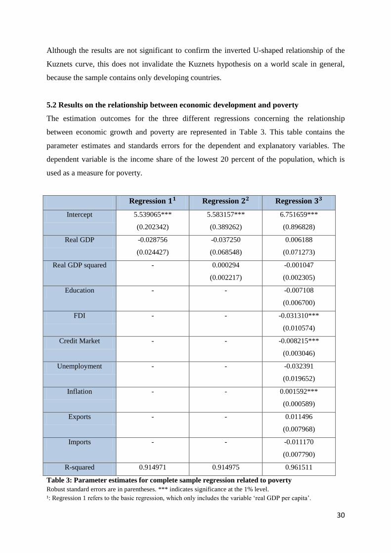
5.2 Results on the relationship between economic development and poverty

The estimation outcomes for the three different regressions concerning the relationship

between economic growth and poverty are represented in Table 3. This table contains the

parameter estimates and standards errors for the dependent and explanatory variables. The

dependent variable is the income share of the lowest 20 percent of the population, which is

used as a measure for poverty.

Regression 𝟏𝟏 Regression 𝟐𝟐 Regression 𝟑𝟑

Intercept 5.539065***

(0.202342)

5.583157***

(0.389262)

6.751659***

(0.896828)

Real GDP -0.028756

(0.024427)

-0.037250

(0.068548)

0.006188

(0.071273)

Real GDP squared - 0.000294

(0.002217)

-0.001047

(0.002305)

Education - - -0.007108

(0.006700)

FDI - - -0.031310***

(0.010574)

Credit Market - - -0.008215***

(0.003046)

Unemployment - - -0.032391

(0.019652)

Inflation - - 0.001592***

(0.000589)

Exports - - 0.011496

(0.007968)

Imports - - -0.011170

(0.007790)

R-squared 0.914971 0.914975 0.961511

Table 3: Parameter estimates for complete sample regression related to poverty

Robust standard errors are in parentheses. *** indicates significance at the 1% level.

¹: Regression 1 refers to the basic regression, which only includes the variable ‘real GDP per capita’.

31

²: Regression 2 extends the basic regression by adding ‘real GDP per capita squared’.

³: Regression 3 extends the second regression by adding control variables.

The parameter estimate for income per capita is negative in the first two regressions, but

becomes positive and much smaller when control variables are added to the regression. The

negative coefficient in the first two regressions implies that an increase in the level of income

per capita will decrease the income share of the lowest 20 percent of the population, i.e. the

relatively poor. The estimate of real GDP per capita in the third regression shows a positive

sign, indicating that economic growth will benefit the poor. This result complies with the

scatter plot in Figure 3. Both outcomes can be in line with the Kuznets curve, since the effect

of income on poverty is uncertain in the early stages of development. The coefficient for

GDP-squared, which measures here the non-linear relationship between income and poverty,

is positive in the basic regression, but becomes negative in the last regression. Thus, there is a

concave relationship between economic growth and income of the poor, when the interaction

is controlled for different variables. However, all parameter estimates for real GDP and real

GDP squared are insignificant and thus have no explanatory power. Therefore, we cannot

assess whether the relationship predicted by Kuznets (1955) holds in the empirical world,

especially for developing countries.

The third regression extends the previous regressions by adding control variables that may

have an impact on the interdependence between economic development and poverty.

Education seems to have a negative effect on the income share of the poorest people in the

population, implying that an increase in the primary completion rate will deteriorate the living

standards of the poor. This result contradicts earlier studies that show the positive effect of

education on earnings. Still, the coefficient is insignificant and thus we cannot accept the

negative relationship between education and poverty.

The parameter estimate for FDI inflows is negative, which indicates that foreign investments

reduce the income share of the poor. In other words, the poorest people of the population do

not benefit from these investments and thus FDI does not seem to be a key factor for poverty

reduction, as shown by earlier studies. Still, the coefficient is significant at the 1% level,

which implies that FDI inflows are an important factor to explain changes in the level of

poverty. The lending interest rate has a negative effect on the living standards of the poor,

which corresponds to the expectation that a higher interest rate decreases the access to credit

32

and thus can lead to a deterioration of the income share of the poor. The coefficient is

significant at the 1% level and thus has a high explanatory power.

The coefficient of the unemployment rate also has a negative sign, implying that an increase

in the level of unemployment leads to a decrease in the income share of the lowest 20 percent

of the population. Although the sign of the variable is in line with earlier expectations, the

coefficient is not significant and thus the unemployment rate cannot serve to explain changes

in poverty.

The inflation rate appears to have a positive impact, meaning that a higher inflation rate will

increase the income share of the poor. This result contradicts earlier studies based on the

interaction between inflation and poverty. Although the estimated result is small, it is

significant at the 1% level, indicating that the degree of poverty is influenced by the inflation

rate. The level of exports has a positive effect on the income of the poor, implying that an

increase in the exports will improve the living standards of the poor. This result corresponds

to theory suggesting that as the degree of exports increases, the returns from trade will shift to

the low-educated and poor people. Still, the estimated result is not significant. Therefore, we

cannot confirm the corresponding interaction between exports and the degree of poverty.

Imports seem to have a negative impact, but the coefficient is insignificant, indicating that the

variable has no explanatory power. Hence, the estimated outcome does not support the

expectation that imports increase the disparity between rich and poor.

The value for R-squared does not really change when GDP-squared is added to the regression.

However, the coefficient does increase from 0.91 to 0.96 when the regression is expanded by

adding control variables that may influence the relationship between economic development

and poverty. This result indicates that the data become closer to the fitted regression line and

thus the independent variables have a high explanatory power for the variation in the income

share of the lowest 20 percent of the population. Nevertheless, it should not be neglected that

R-squared usually increases when more variables are added to the regression.

As mentioned before, the insignificant results belong only to the sample of developing

countries and thus cannot invalidate the Kuznets theory on a world scale.

33

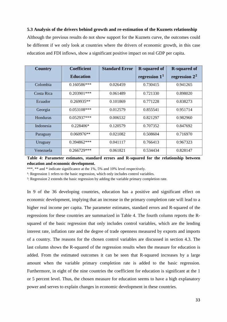
5.3 Analysis of the drivers behind growth and re-estimation of the Kuznets relationship

Although the previous results do not show support for the Kuznets curve, the outcomes could

be different if we only look at countries where the drivers of economic growth, in this case

education and FDI inflows, show a significant positive impact on real GDP per capita.

Country Coefficient

Education

Standard Error R-squared of

regression 𝟏𝟏

R-squared of

regression 𝟐𝟐

Colombia 0.160586*** 0.026459 0.730415 0.941265

Costa Rica 0.203901*** 0.061489 0.721330 0.898020

Ecuador 0.269935** 0.101869 0.771228 0.838273

Georgia 0.053108*** 0.012579 0.855541 0.951714

Honduras 0.052937*** 0.006532 0.821297 0.982960

Indonesia 0.228406* 0.120579 0.707352 0.847692

Paraguay 0.060976** 0.021082 0.508604 0.716970

Uruguay 0.394862*** 0.041117 0.766413 0.967323

Venezuela 0.266729*** 0.061821 0.534434 0.828147

Table 4: Parameter estimates, standard errors and R-squared for the relationship between

education and economic development.

***, ** and * indicate significance at the 1%, 5% and 10% level respectively.

¹: Regression 1 refers to the basic regression, which only includes control variables.

²: Regression 2 extends the basic regression by adding the variable primary completion rate.

In 9 of the 36 developing countries, education has a positive and significant effect on

economic development, implying that an increase in the primary completion rate will lead to a

higher real income per capita. The parameter estimates, standard errors and R-squared of the

regressions for these countries are summarized in Table 4. The fourth column reports the R-

squared of the basic regression that only includes control variables, which are the lending

interest rate, inflation rate and the degree of trade openness measured by exports and imports

of a country. The reasons for the chosen control variables are discussed in section 4.3. The

last column shows the R-squared of the regression results when the measure for education is

added. From the estimated outcomes it can be seen that R-squared increases by a large

amount when the variable primary completion rate is added to the basic regression.

Furthermore, in eight of the nine countries the coefficient for education is significant at the 1

or 5 percent level. Thus, the chosen measure for education seems to have a high explanatory

power and serves to explain changes in economic development in these countries.

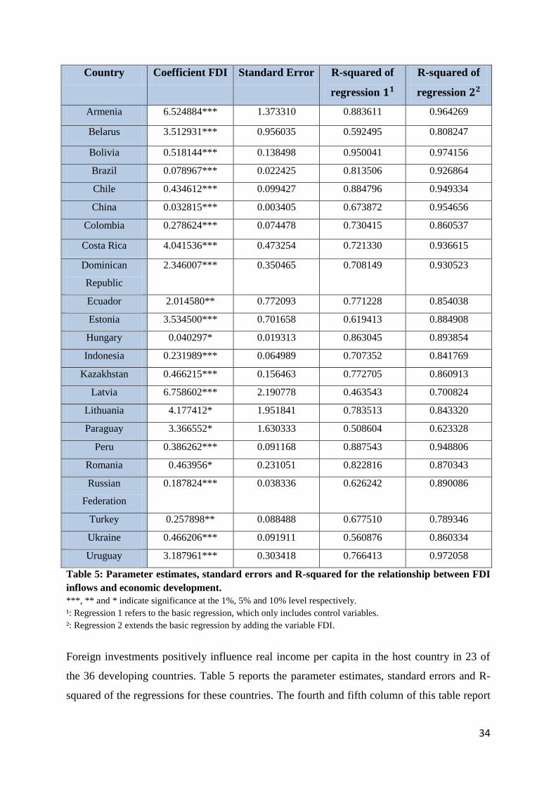
34

Country Coefficient FDI Standard Error R-squared of

regression 𝟏𝟏

R-squared of

regression 𝟐𝟐

Armenia 6.524884*** 1.373310 0.883611 0.964269

Belarus 3.512931*** 0.956035 0.592495 0.808247

Bolivia 0.518144*** 0.138498 0.950041 0.974156

Brazil 0.078967*** 0.022425 0.813506 0.926864

Chile 0.434612*** 0.099427 0.884796 0.949334

China 0.032815*** 0.003405 0.673872 0.954656

Colombia 0.278624*** 0.074478 0.730415 0.860537

Costa Rica 4.041536*** 0.473254 0.721330 0.936615

Dominican

Republic

2.346007*** 0.350465 0.708149 0.930523

Ecuador 2.014580** 0.772093 0.771228 0.854038

Estonia 3.534500*** 0.701658 0.619413 0.884908

Hungary 0.040297* 0.019313 0.863045 0.893854

Indonesia 0.231989*** 0.064989 0.707352 0.841769

Kazakhstan 0.466215*** 0.156463 0.772705 0.860913

Latvia 6.758602*** 2.190778 0.463543 0.700824

Lithuania 4.177412* 1.951841 0.783513 0.843320

Paraguay 3.366552* 1.630333 0.508604 0.623328

Peru 0.386262*** 0.091168 0.887543 0.948806

Romania 0.463956* 0.231051 0.822816 0.870343

Russian

Federation

0.187824*** 0.038336 0.626242 0.890086

Turkey 0.257898** 0.088488 0.677510 0.789346

Ukraine 0.466206*** 0.091911 0.560876 0.860334

Uruguay 3.187961*** 0.303418 0.766413 0.972058

Table 5: Parameter estimates, standard errors and R-squared for the relationship between FDI

inflows and economic development.

***, ** and * indicate significance at the 1%, 5% and 10% level respectively.

¹: Regression 1 refers to the basic regression, which only includes control variables.

²: Regression 2 extends the basic regression by adding the variable FDI.

Foreign investments positively influence real income per capita in the host country in 23 of

the 36 developing countries. Table 5 reports the parameter estimates, standard errors and R-

squared of the regressions for these countries. The fourth and fifth column of this table report

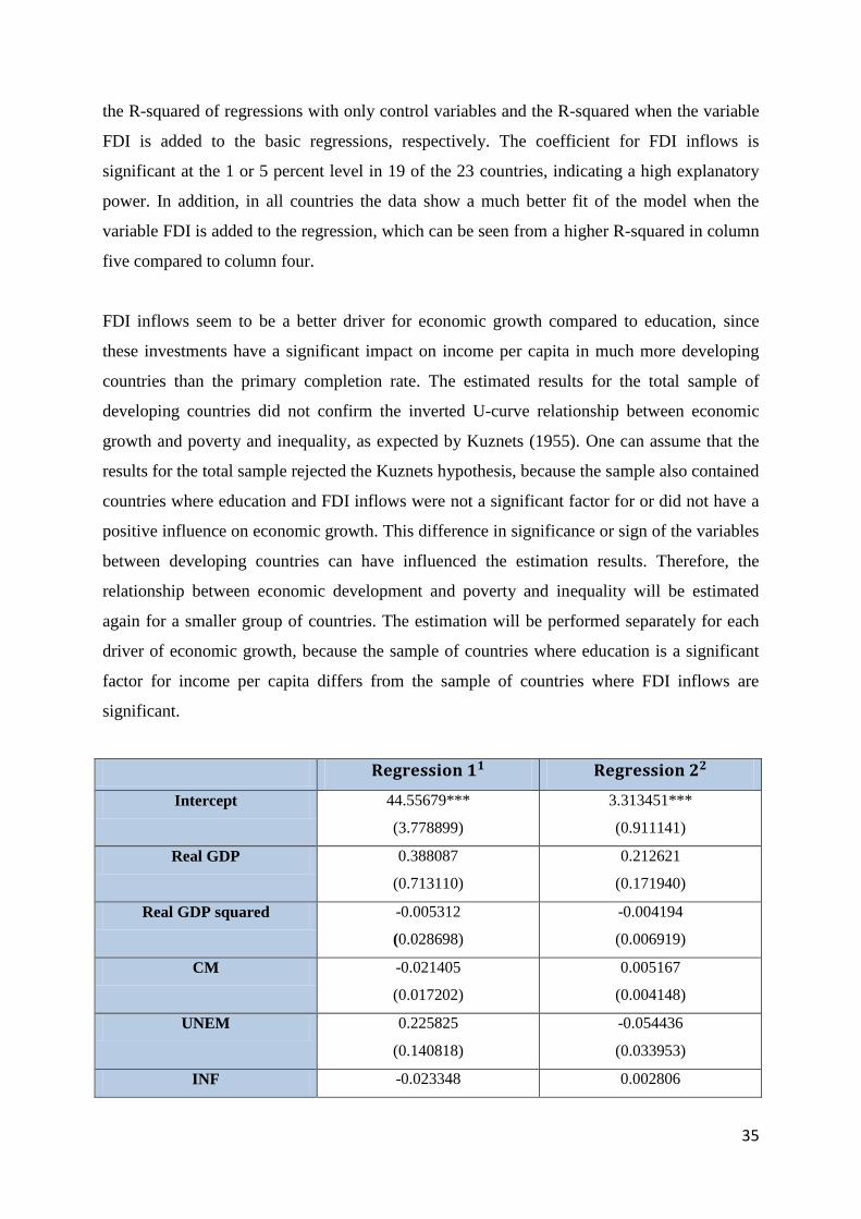
35

the R-squared of regressions with only control variables and the R-squared when the variable

FDI is added to the basic regressions, respectively. The coefficient for FDI inflows is

significant at the 1 or 5 percent level in 19 of the 23 countries, indicating a high explanatory

power. In addition, in all countries the data show a much better fit of the model when the

variable FDI is added to the regression, which can be seen from a higher R-squared in column

five compared to column four.

FDI inflows seem to be a better driver for economic growth compared to education, since

these investments have a significant impact on income per capita in much more developing

countries than the primary completion rate. The estimated results for the total sample of

developing countries did not confirm the inverted U-curve relationship between economic

growth and poverty and inequality, as expected by Kuznets (1955). One can assume that the

results for the total sample rejected the Kuznets hypothesis, because the sample also contained

countries where education and FDI inflows were not a significant factor for or did not have a

positive influence on economic growth. This difference in significance or sign of the variables

between developing countries can have influenced the estimation results. Therefore, the

relationship between economic development and poverty and inequality will be estimated

again for a smaller group of countries. The estimation will be performed separately for each

driver of economic growth, because the sample of countries where education is a significant

factor for income per capita differs from the sample of countries where FDI inflows are

significant.

𝐑𝐞𝐠𝐫𝐞𝐬𝐬𝐢𝐨𝐧 𝟏𝟏 𝐑𝐞𝐠𝐫𝐞𝐬𝐬𝐢𝐨𝐧 𝟐𝟐

Intercept 44.55679***

(3.778899)

3.313451***

(0.911141)

Real GDP 0.388087

(0.713110)

0.212621

(0.171940)

Real GDP squared -0.005312

(0.028698)

-0.004194

(0.006919)

CM -0.021405

(0.017202)

0.005167

(0.004148)

UNEM 0.225825

(0.140818)

-0.054436

(0.033953)

INF -0.023348 0.002806

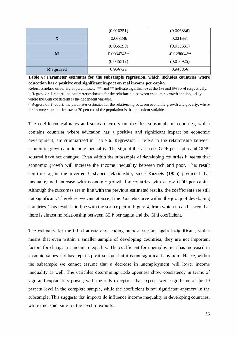
36

(0.028351) (0.006836)

X -0.063349

(0.055290)

0.021651

(0.013331)

M 0.093434**

(0.045312)

-0.028004**

(0.010925)

R-squared 0.956722 0.948856

Table 6: Parameter estimates for the subsample regression, which includes countries where

education has a positive and significant impact on real income per capita.

Robust standard errors are in parentheses. *** and ** indicate significance at the 1% and 5% level respectively.

¹: Regression 1 reports the parameter estimates for the relationship between economic growth and inequality,

where the Gini coefficient is the dependent variable.

²: Regression 2 reports the parameter estimates for the relationship between economic growth and poverty, where

the income share of the lowest 20 percent of the population is the dependent variable.

The coefficient estimates and standard errors for the first subsample of countries, which

contains countries where education has a positive and significant impact on economic

development, are summarized in Table 6. Regression 1 refers to the relationship between

economic growth and income inequality. The sign of the variables GDP per capita and GDP-

squared have not changed. Even within the subsample of developing countries it seems that

economic growth will increase the income inequality between rich and poor. This result

confirms again the inverted U-shaped relationship, since Kuznets (1955) predicted that

inequality will increase with economic growth for countries with a low GDP per capita.

Although the outcomes are in line with the previous estimated results, the coefficients are still

not significant. Therefore, we cannot accept the Kuznets curve within the group of developing

countries. This result is in line with the scatter plot in Figure 4, from which it can be seen that

there is almost no relationship between GDP per capita and the Gini coefficient.

The estimates for the inflation rate and lending interest rate are again insignificant, which

means that even within a smaller sample of developing countries, they are not important

factors for changes in income inequality. The coefficient for unemployment has increased in

absolute values and has kept its positive sign, but it is not significant anymore. Hence, within

the subsample we cannot assume that a decrease in unemployment will lower income

inequality as well. The variables determining trade openness show consistency in terms of

sign and explanatory power, with the only exception that exports were significant at the 10

percent level in the complete sample, while the coefficient is not significant anymore in the

subsample. This suggests that imports do influence income inequality in developing countries,

while this is not sure for the level of exports.

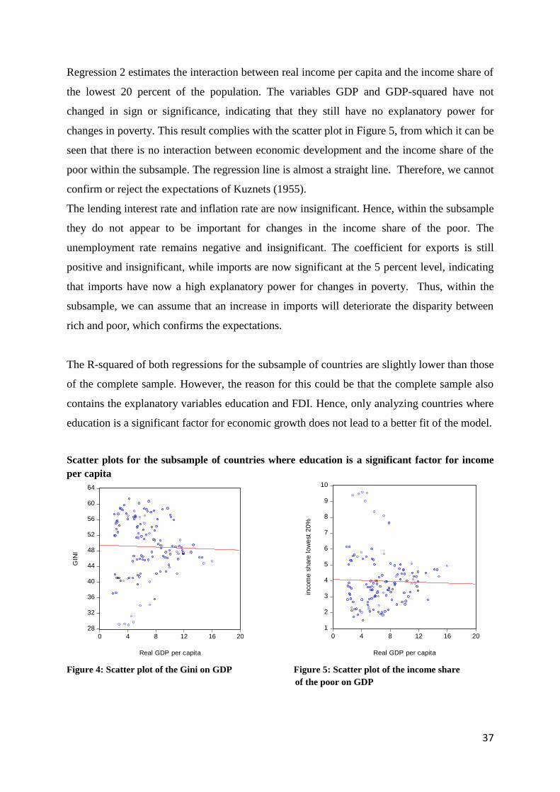
37

Regression 2 estimates the interaction between real income per capita and the income share of

the lowest 20 percent of the population. The variables GDP and GDP-squared have not

changed in sign or significance, indicating that they still have no explanatory power for

changes in poverty. This result complies with the scatter plot in Figure 5, from which it can be

seen that there is no interaction between economic development and the income share of the

poor within the subsample. The regression line is almost a straight line. Therefore, we cannot

confirm or reject the expectations of Kuznets (1955).

The lending interest rate and inflation rate are now insignificant. Hence, within the subsample

they do not appear to be important for changes in the income share of the poor. The

unemployment rate remains negative and insignificant. The coefficient for exports is still

positive and insignificant, while imports are now significant at the 5 percent level, indicating

that imports have now a high explanatory power for changes in poverty. Thus, within the

subsample, we can assume that an increase in imports will deteriorate the disparity between

rich and poor, which confirms the expectations.

The R-squared of both regressions for the subsample of countries are slightly lower than those

of the complete sample. However, the reason for this could be that the complete sample also

contains the explanatory variables education and FDI. Hence, only analyzing countries where

education is a significant factor for economic growth does not lead to a better fit of the model.

Scatter plots for the subsample of countries where education is a significant factor for income

per capita

28

32

36

40

44

48

52

56

60

64

0 4 8 12 16 20

Real GDP per capita

GIN

I

1

2

3

4

5

6

7

8

9

10

0 4 8 12 16 20

Real GDP per capita

incom

e s

ha

re lo

west

20%

Figure 4: Scatter plot of the Gini on GDP Figure 5: Scatter plot of the income share

of the poor on GDP

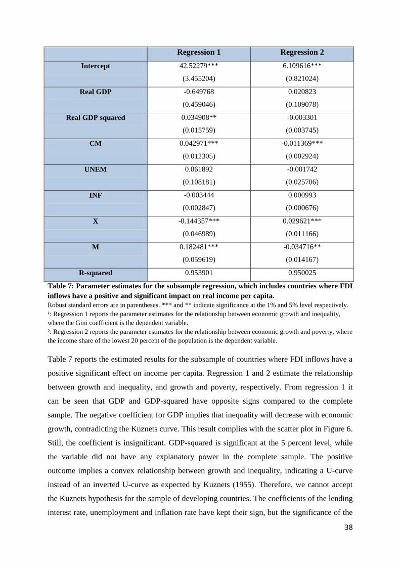
38

Regression 1 Regression 2

Intercept 42.52279***

(3.455204)

6.109616***

(0.821024)

Real GDP -0.649768

(0.459046)

0.020823

(0.109078)

Real GDP squared 0.034908**

(0.015759)

-0.003301

(0.003745)

CM 0.042971***

(0.012305)

-0.011369***

(0.002924)

UNEM 0.061892

(0.108181)

-0.001742

(0.025706)

INF -0.003444

(0.002847)

0.000993

(0.000676)

X -0.144357***

(0.046989)

0.029621***

(0.011166)

M 0.182481***

(0.059619)

-0.034716**

(0.014167)

R-squared 0.953901 0.950025

Table 7: Parameter estimates for the subsample regression, which includes countries where FDI

inflows have a positive and significant impact on real income per capita.

Robust standard errors are in parentheses. *** and ** indicate significance at the 1% and 5% level respectively.

¹: Regression 1 reports the parameter estimates for the relationship between economic growth and inequality,

where the Gini coefficient is the dependent variable.

²: Regression 2 reports the parameter estimates for the relationship between economic growth and poverty, where

the income share of the lowest 20 percent of the population is the dependent variable.

Table 7 reports the estimated results for the subsample of countries where FDI inflows have a

positive significant effect on income per capita. Regression 1 and 2 estimate the relationship

between growth and inequality, and growth and poverty, respectively. From regression 1 it

can be seen that GDP and GDP-squared have opposite signs compared to the complete

sample. The negative coefficient for GDP implies that inequality will decrease with economic

growth, contradicting the Kuznets curve. This result complies with the scatter plot in Figure 6.

Still, the coefficient is insignificant. GDP-squared is significant at the 5 percent level, while

the variable did not have any explanatory power in the complete sample. The positive

outcome implies a convex relationship between growth and inequality, indicating a U-curve

instead of an inverted U-curve as expected by Kuznets (1955). Therefore, we cannot accept

the Kuznets hypothesis for the sample of developing countries. The coefficients of the lending

interest rate, unemployment and inflation rate have kept their sign, but the significance of the

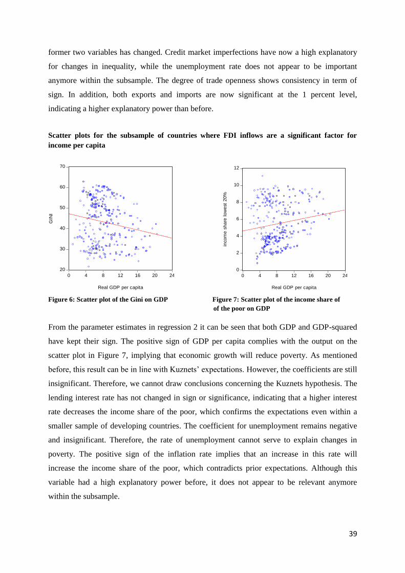
39

former two variables has changed. Credit market imperfections have now a high explanatory

for changes in inequality, while the unemployment rate does not appear to be important

anymore within the subsample. The degree of trade openness shows consistency in term of

sign. In addition, both exports and imports are now significant at the 1 percent level,

indicating a higher explanatory power than before.

Scatter plots for the subsample of countries where FDI inflows are a significant factor for

income per capita

20

30

40

50

60

70

0 4 8 12 16 20 24

Real GDP per capita

GIN

I

0

2

4

6

8

10

12

0 4 8 12 16 20 24

Real GDP per capita

inco

me

sh

are

lo

we

st

20

%

Figure 6: Scatter plot of the Gini on GDP Figure 7: Scatter plot of the income share of

of the poor on GDP

From the parameter estimates in regression 2 it can be seen that both GDP and GDP-squared

have kept their sign. The positive sign of GDP per capita complies with the output on the

scatter plot in Figure 7, implying that economic growth will reduce poverty. As mentioned

before, this result can be in line with Kuznets’ expectations. However, the coefficients are still

insignificant. Therefore, we cannot draw conclusions concerning the Kuznets hypothesis. The

lending interest rate has not changed in sign or significance, indicating that a higher interest

rate decreases the income share of the poor, which confirms the expectations even within a

smaller sample of developing countries. The coefficient for unemployment remains negative

and insignificant. Therefore, the rate of unemployment cannot serve to explain changes in

poverty. The positive sign of the inflation rate implies that an increase in this rate will

increase the income share of the poor, which contradicts prior expectations. Although this

variable had a high explanatory power before, it does not appear to be relevant anymore

within the subsample.

40

The degree of trade openness seems to influence the income share of the poor. Hence, within

the subsample we can assume that as the degree of exports increases, the returns from trade

will shift to the poor. Furthermore, higher imports will benefit the rich and increase the

disparity between rich and poor.

The R-squared of the regressions for the subsample are slightly lower than those for the

complete sample. Still, we cannot conclude that the complete sample leads to a better fit of

the model, since the regression for the complete sample also contains the variables education

and FDI. As mentioned before, R-squared usually increases when more variables are added to

the regression.

Even though the sample was divided into subsamples to prove the existence of a Kuznets

curve within developing countries, the results do not show sufficient support for an inverted

U-curve.

41

VI: CONCLUSION

This paper aims to contribute to the existing literature on the Kuznets curve by investigating

the effect of the level of real GDP per capita on poverty and income inequality. This set-up is

different from previous studies which have focused on the reverse relationship. The sample of

countries examined contains only developing nations, mainly due to a high poverty and

inequality in these countries. According to theory, this group of countries is located on the left

side of the Kuznets curve, which indicates that the effect of income per capita on inequality

must be consistently positive.

The expected relationship between economic growth and income inequality seems to not hold

in reality. The regression results for the complete sample of developing countries are

consistent in terms of sign of the GDP coefficient and confirm the Kuznets curve, but the

observed relationship is insignificant. When re-estimating the relationship for subsamples, the

coefficient for GDP keeps its positive sign within the sample where education is a significant

driver for economic growth, while it has a negative sign when only analyzing countries where

FDI inflows affect income per capita. Still, the variable remains insignificant in both

subsamples. The estimated results for the interaction between economic growth and poverty

can be in line with the expectations of the Kuznets hypothesis. The positive relationship holds

for both the complete sample and the subsamples, but the coefficient is insignificant in all

estimations. Hence, the sample of developing countries does not show sufficient evidence for

the existence of the Kuznets curve. The level of income seems to have no explanatory power

for changes in inequality or poverty. Thus, economic growth in developing countries will not

reduce the disparity between rich and poor. Still, this does not invalidate the Kuznets

hypothesis on a world scale in general, because the sample contains only developing nations.

Since the results are insignificant, it is not possible to draw conclusions and give suggestions

about how policies must be tailored to countries’ specificities in order to make the income

distribution more even. Nevertheless, this paper has some undoubted merits, such as its focus

on developing countries only. While the Kuznets curve as such has substantial theoretical and,

perhaps less often, empirical evidence, its validity has not been explored much on a sample of

developing countries only. Furthermore, the research considers very recent data (1990-2010).

42

There are some drawbacks in this research and these may have influenced the rigorousness of

the results. There was missing data for many countries and this forced the selection of only a

subset of developing countries. A larger and relatively more homogeneous sample may be

able to display a Kuznets curve or at least provide evidence of a significant positive

relationship between the main variables. In addition, the regression can be expanded by the

inclusion of more explanatory variables, for instance accounting for political climate and

social unrest. These shortcomings provide sufficient room for further research.

43

VII: BIBLIOGRAPHY

Aaberge, R., Björklund, A., Jäntti, M., Pedersen, P.J., Smith, N., Wennemo, T. (2000). Unemployment

Shocks and Income Distribution: How did the Nordic Countries Fare during their Crises?

Scandinavian Journal of Economics, 102(1), 77-99.

Albanesi, S. (2006). Inflation and inequality. Journal of Monetary Economics, 54(4), 1088-1114.

Alfaro, L., Chanda, A., Kalemli-Ozcan, S., & Sayek, S. (2004). FDI and economic growth: the role of

local financial markets. Journal of international economics, 64(1), 89-112.

Azevedo, J.P., Inchauste, G., & Sanfelice, V. (2013). Decomposing the Recent Inequality Decline

in Latin America. World Bank Policy Research Working Paper ,6715.

Banerjee, A.V., & Duflo, E. (2003). Inequality and growth: What can the data say?. Journal of

economic growth, 8(3), 267-299.

Barro, R.J. (1999). Inequality, growth and investment. National bureau of economic research, w7038.

Barro, R.J. (2000). Inequality and Growth in a Panel of Countries. Journal of economic growth, 5(1),

5-32.

Berg, S. van der. (2008). Poverty and education. Education policy series, 10.

Cardoso, E. (1992). Inflation and poverty. National Bureau of Economic Research, w4006.

Cohen, W. M., & Levinthal, D. A. (1990). Absorptive capacity: a new perspective on learning and

innovation. Administrative science quarterly, 35, 128-152.

Davis, D. R. (1996). Trade liberalization and income distribution. National bureau of economic

research, w5693.

Deininger, K., & Squire, L. (1998). New ways of looking at old issues: inequality and growth. Journal

of development economics, 57(2), 259-287.

44

Dollar, D., & Kraay, A. (2002). Growth is Good for the Poor. Journal of economic growth, 7(3), 195-

225.

Duménil, G., & Lévy, D. (2013) The Crisis of Neoliberalism. Harvard University Press.

Fischer, S. (1993). The role of macroeconomic factors in growth. Journal of monetary

economics, 32(3), 485-512.

Forbes, K. J. (2000). A Reassessment of the Relationship between Inequality and Growth. American

economic review, 90(4), 869-887.

Gregorio, J. D., & Lee, J. W. (1999). Education and income distribution: new evidence from cross-

country data. No.55.

Hanushek, E. A., & Wößmann, L. (2007). The role of education quality for economic growth. World

Bank Policy Research Working Paper, 4122.

Harrison, A. (1996). Openness and growth: A time-series, cross-country analysis for developing

countries. Journal of development Economics, 48(2), 419-447.

Klein, M. U., Aaron, C., & Hadjimichael, B. (2001). Foreign direct investment and poverty reduction.

World Bank Publications, 2613.

Kremer, M., Bovens, M., Schrijvers, E., & Went, R. (2014). Hoe ongelijk is Nederland? Een

verkenning van de ontwikkeling en gevolgen van economische ongelijkheid. Amsterdam University

Press.

Krueger, A. B., & Lindahl, M. (2000). Education for growth: why and for whom? National Bureau of

Economic Research, w7591.

Kuznets, S. (1955). Economic growth and income inequality. The American economic review, 45(1),

1-28.

Li, H., & Zou, H. F. (1998). Income inequality is not harmful for growth: theory and evidence. Review

of Development Economics, 2(3), 318-334.

45

Milanovic, B. (1994). Determinants of cross-country income inequality: an augmented Kuznets

hypothesis. The World Bank, 1246.

Moran, T.P. (2005). Kuznets’s inverted U-curve hypothesis: The rise, demise, and continued relevance

of a socioeconomic law. Sociological Forum, 20(2), 209-244.

Perotti, R. (1996). Growth, income distribution, and democracy: what the data say. Journal of

Economic growth, 1(2), 149-187.

Ravallion, M. (1995). Growth and poverty: evidence for developing countries in the 1980s. Economics

letters, 48(3), 411-417.

Roemer, M., & Gugerty, M. K. (1997). Does economic growth reduce poverty? CAER II.

The World Bank (2014), Retrieved from: www.data.worldbank.org

UN (2013) Inequality Matters: Report on the World Social Situation 2013. New York: United

Nations.

Wu, J.Y. & Hsu, C.C. (2012). Foreign direct investment and income inequality: Does the relationship

vary with absorptive capacity? Economic modeling, 29 (6), 2183-2189