Embed Size (px)
Citation preview

Department of Economics
Working Paper No. 176
Can Macroeconomists Get Rich
Forecasting Exchange Rates?
Mauro Costantini Jesus Crespo Cuaresma
Jaroslava Hlouskova
June 2014

Can Macroeconomists Get Rich
Forecasting Exchange Rates?∗
Mauro Costantini†
Jesus Crespo Cuaresma‡
Jaroslava Hlouskova§
Abstract
We provide a systematic comparison of the out-of-sample forecasts based on multivariate macroe-
conomic models and forecast combinations for the euro against the US dollar, the British pound,
the Swiss franc and the Japanese yen. We use profit maximization measures based on directional
accuracy and trading strategies in addition to standard loss minimization measures. When com-
paring predictive accuracy and profit measures, data snooping bias free tests are used. The results
indicate that forecast combinations help to improve over benchmark trading strategies for the
exchange rate against the US dollar and the British pound, although the excess return per unit
of deviation is limited. For the euro against the Swiss franc or the Japanese yen, no evidence of
generalized improvement in profit measures over the benchmark is found.
JEL codes: C53, F31, F37
Keywords: Exchange rate forecasting, forecast combination, multivariate time series models, profitability
∗The research in this paper was supported by the Anniversary Fund of the Austrian Central Bank (ProjectNo. 15308). The authors would like to thank Robert Kunst for thoughtful comments and remarks.
†Department of Economics and Finance, Brunel University, London, UK‡Department of Economics, Vienna University of Economics and Business; Wittgenstein Centre for Demogra-
phy and Global Human Capital (WIC); World Population Program, International Institute of Applied SystemsAnalysis (IIASA) and Austrian Institute for Economic Research (WIFO), Vienna, Austria
§Department of Economics and Finance, Institute for Advanced Studies, Vienna, Austria, and Departmentof Economics, Thompson Rivers University, Kamloops, BC, Canada

1 Introduction
Forecasting exchange rates is a notoriously difficult task. Myriads of empirical studies (see
for example the recent survey by James et al., 2012) document the challenges associated with
specifying macro-econometric models with good predictive performance for exchange rate data,
in particular for short-run forecasting horizons.
Since the seminal work by Meese and Rogoff (1983), which shows that specifications based
on macroeconomic fundamentals are unable to outperform simple random walk forecasts, a large
number of studies have proposed models aimed at providing accurate out-of-sample predictions
of spot exchange rates (see MacDonald and Taylor, 1994; Mark, 1995; Chinn and Meese, 1995;
Kilian, 1999; Mark and Sul, 2001; Berkowitz and Giorgianni, 2001; Cheung et al.; 2005, or
Boudoukh et al., 2008, among others). In parallel, a literature has emerged which examines
empirically the potential profitability of technical trading rules (see Menkhoff and Taylor, 2007,
for a review). The analysis of profitability of technical trading rules can be thought of as a
simple and robust test for the weak form of the efficient market hypothesis, which concludes
that if the foreign exchange market is efficient, one should not be able to use publicly available
information to correctly forecast changes in exchange rates and thus make an abnormal profit.
The aim of this paper is to provide a systematic comparison of out-of-sample forecast accu-
racy in terms of predictive error, directional accuracy and profitability of trading strategies for
the euro against the US dollar, the British pound, the Swiss franc and the Japanese yen. To the
best of our knowledge, the closest paper to ours is Yang et al. (2008), who applied the nonlinear
approach of Hong and Lee (2003) to test the martingale hypothesis of the daily euro exchange
rate against seven currencies. However, our analysis differs from theirs in many respects. First,
we use monthly data and apply several multivariate macro-econometric models.1 Second, in
addition to standard loss measures based on prediction errors, recently developed directional
forecast accuracy measures are also considered. The latter measures account for both the real-
ized directional changes in exchange rates as well as for their magnitudes (see Blaskowitz and
Herwartz, 2009, 2011; Bergmeir et al., 2014). This is the first innovation of the paper relative to
the existing literature. Such measures are robust to outliers and provide an economically inter-
pretable loss/success functional framework in a decision-theoretical context, which is extremely
relevant for traders and investors. Third, this paper not only tests for the predictability of the
euro exchange rate based on both loss and directional accuracy measures using a benchmark
random walk model, but it also compares the (risk adjusted) profits generated by forecast-based
1Yang et al. (2008), on the other hand, use daily data and thus suggest exploring the predictability of theeuro exchange rate for a different frequency.
2

trading strategies to those using benchmark trading rules. The comparison of predictive accu-
racy and profit measures is assessed using the following data snooping bias free tests that are
based on extensive bootstrap-based procedure: the ‘reality check’ (RC) test of White (2000),
the test for superior predictive ability (SPA) by Hansen (2005), the stepwise test of multiple
reality check (StepM-RC) by Romano and Wolf (2005) and the stepwise multiple superior pre-
dictive ability (StepM-SPA) test by Hsu et al. (2010). Fourth, and this is the second novelty
of the paper, we exploit the potential of a large number of forecast combination methods for
both forecast accuracy evaluation and profitability. In doing so, we propose a new method of
combination based on the economic evaluation of directional forecasts. The other methods of
combination used are the mean, median or trimmed mean, the ordinary least squares combining
methods, combinations based, on principal components, on discounted mean square forecast
errors, on hit rates and on Bayesian and frequentist model averaging techniques are considered.
The results of our analysis indicate that forecast combinations, and in particular forecast
pooling based on principal components, tend to improve profitability of trading rules as com-
pared to benchmark strategies and strategies based on single multivariate time series specifica-
tions for the EUR/USD and EUR/GBP rates. Such an improvement, however, is by no means
systematic across profitability measures and forecasting horizons. In addition, the comparison
of the realized Sharpe ratios reveals that the margin for achieving systematic profits in the
foreign exchange market using the information contained by macroeconomic variables is very
small. On the other hand, the forecasts of the EUR/CHF exchange rate based on both individ-
ual models and forecast combinations do outperform the random walk model for a long-term
prediction horizon. For the case of the EUR/JPY exchange rates, on the other hand, we find
no robust improvement over standard benchmarks.
The rest of the paper is organized as follows. Section 2 describes the analytical framework
used, including the forecast combination approaches and the forecast accuracy measures, as well
as the trading strategies they are based on. In section 3, the design of the empirical exercise
and the testing procedures for data snooping biases are presented. The results are discussed in
section 4 and section 5 concludes.
2 Analytical framework
2.1 The monetary model of exchange rates
The theoretical framework of the monetary model of exchange rate formation (for the original
formulations, see Frenkel, 1976; Dornbusch, 1976; Hooper and Morton, 1982) has become the
3
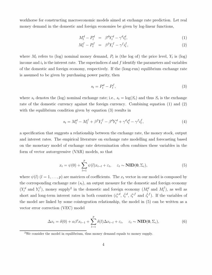
workhorse for constructing macroeconomic models aimed at exchange rate prediction. Let real
money demand in the domestic and foreign economies be given by log-linear functions,
Mdt − P d
t = βdY dt − γdidt , (1)
Mft − P f
t = βfY ft − γf ift , (2)
where Mt refers to (log) nominal money demand, Pt is (the log of) the price level, Yt is (log)
income and it is the interest rate. The superindices d and f identify the parameters and variables
of the domestic and foreign economy, respectively. If the (long-run) equilibrium exchange rate
is assumed to be given by purchasing power parity, then
st = P dt − P f
t , (3)
where st denotes the (log) nominal exchange rate; i.e., st = log(St) and thus St is the exchange
rate of the domestic currency against the foreign currency. Combining equation (1) and (2)
with the equilibrium condition given by equation (3) results in
st =Mdt −Mf
t + βfY ft − βdY d
t + γdidt − γf ift , (4)
a specification that suggests a relationship between the exchange rate, the money stock, output
and interest rates. The empirical literature on exchange rate modelling and forecasting based
on the monetary model of exchange rate determination often combines these variables in the
form of vector autoregressive (VAR) models, so that
xt = ψ(0) +
p∑
l=1
ψ(l)xt−l + εt, εt ∼ NID(0,Σε), (5)
where ψ(l) (l = 1, . . . , p) are matrices of coefficients. The xt vector in our model is composed by
the corresponding exchange rate (st), an output measure for the domestic and foreign economy
(Y dt and Y f
t ), money supply2 in the domestic and foreign economy (Mdt and Mf
t ), as well as
short and long-term interest rates in both countries (is,dt , il,dt , is,ft and il,ft ). If the variables of
the model are linked by some cointegration relationship, the model in (5) can be written as a
vector error correction (VEC) model
∆xt = δ(0) + αβ ′xt−1 +
p∑
l=1
δ(l)∆xt−l + εt, εt ∼ NID(0,Σε), (6)
2We consider the model in equilibrium, thus money demand equals to money supply.
4
where the cointegration relationships are given by β ′xt and α measures the speed of adjustment
to the long run equilibrium. Alternatively, if the variables in xt are unit-root nonstationary
but no cointegration relationship exists among them, a VAR model in first differences (DVAR)
would be the appropriate representation,
∆xt = ψ(0) +
p−1∑
l=1
ψ(l)∆xt−l + εt, εt ∼ NID(0,Σε). (7)
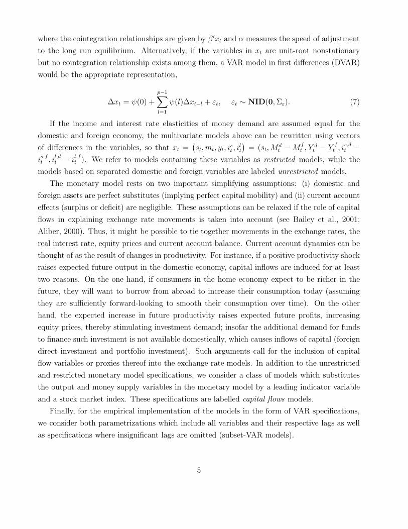
If the income and interest rate elasticities of money demand are assumed equal for the
domestic and foreign economy, the multivariate models above can be rewritten using vectors
of differences in the variables, so that xt =(
st, mt, yt, ist , i
lt
)
= (st,Mdt −Mf
t , Ydt − Y f
t , is,dt −
is,ft , il,dt − il,ft ). We refer to models containing these variables as restricted models, while the
models based on separated domestic and foreign variables are labeled unrestricted models.
The monetary model rests on two important simplifying assumptions: (i) domestic and
foreign assets are perfect substitutes (implying perfect capital mobility) and (ii) current account
effects (surplus or deficit) are negligible. These assumptions can be relaxed if the role of capital
flows in explaining exchange rate movements is taken into account (see Bailey et al., 2001;
Aliber, 2000). Thus, it might be possible to tie together movements in the exchange rates, the
real interest rate, equity prices and current account balance. Current account dynamics can be
thought of as the result of changes in productivity. For instance, if a positive productivity shock
raises expected future output in the domestic economy, capital inflows are induced for at least
two reasons. On the one hand, if consumers in the home economy expect to be richer in the
future, they will want to borrow from abroad to increase their consumption today (assuming
they are sufficiently forward-looking to smooth their consumption over time). On the other
hand, the expected increase in future productivity raises expected future profits, increasing
equity prices, thereby stimulating investment demand; insofar the additional demand for funds
to finance such investment is not available domestically, which causes inflows of capital (foreign
direct investment and portfolio investment). Such arguments call for the inclusion of capital
flow variables or proxies thereof into the exchange rate models. In addition to the unrestricted
and restricted monetary model specifications, we consider a class of models which substitutes
the output and money supply variables in the monetary model by a leading indicator variable
and a stock market index. These specifications are labelled capital flows models.
Finally, for the empirical implementation of the models in the form of VAR specifications,
we consider both parametrizations which include all variables and their respective lags as well
as specifications where insignificant lags are omitted (subset-VAR models).
5

2.2 Forecasts and combinations
The aim of our analysis is to assess the profitability of trading strategies based on out-of-
sample predictions of individual VAR, VEC and DVAR models, as well as combinations of
these. Let us denote Si,t+h|t the exchange rate forecast obtained using model i, i = 1, . . . , k, for
time t + h conditional on the information available at time t (i.e., h is the forecast horizon).
Pooled forecasts, Sc,t+h|t, take the form of a linear combination of the predictions of individual
specifications,
Sc,t+h|t = whc,0t +
k∑
i=1
whc,itSi,t+h|t, (8)
where c is the combination method, k is the number of individual forecasts and the weights are
given by {whc,it}ki=0.
Since several combination methods require statistics based on a hold-out sample, let us
introduce here some notation on the subsample limits: T0 is used to denote the first observation
of the available sample, the interval (T1, T2) is used as a hold-out sample used to obtain weights
for those methods where such a subsample is required and T3 is the last available observation.
The sample given by (T2, T3) is the proper out-of-sample period used to compare the different
methods.
We consider a large number of combination methods proposed in the literature:
(i) Mean, trimmed mean, median. With regard to the mean, whmean,0t = 0 and wh
mean,it =1kin
equation (8). The trimmed mean uses whtrim,0t = 0 and wh
trim,it = 0 for the individual mod-
els that generate the smallest and largest forecasts, while whtrim,it =
1k−2
for the remaining
individual models. For the median combination method, Sc,t+h|t = median{Si,t+h|t}ki=1 is
used (see Costantini and Pappalardo, 2010).
(ii) Ordinary least squares (OLS) combination (see Granger and Ramanathan, 1984). The
method estimates the parameters in equation (8) using recursive and rolling windows. In
the recursive case, to compute the initial OLS combination forecast, for ST2 , we regress
{St+h}T2−2ht=T1−1 on a constant and {Si,t+h|t}T2−2h
t=T1−1, i = 1, . . . , k, and set the weights in
equation (8), whOLS,i,T2−h, equal to the estimated OLS coefficients. To construct the sec-
ond combination forecast, for ST2+1, the OLS coefficients are estimated by regressing
{St+h}T2−2h+1t=T1−1 on a constant and {Si,t+h|t}T2−2h+1
t=T1−1 , i = 1, . . . , k, and the fitted OLS coeffi-
cients, whOLS,i,T2−h+1, are used as weights for equation (8). This procedure is applied until
the available out-of-sample period; i.e., the weights of the h−step ahead forecast for ST3
are obtained by regressing {St+h}T3−2ht=T1−1 on a constant and {Si,t+h|t}T3−2h
t=T1−1, i = 1, . . . , k.
6

In the case of the rolling window, we proceed in a similar fashion but discard the first
observations in each replication of the procedure, so that the time series are consistently
of length T2 − T1 − 2h + 2. Thus, for the second combination forecast ST2+1, for in-
stance, we regress {St+h}T2−2h+1t=T1
on a constant and {Si,t+h|t}T2−2h+1t=T1
, i = 1, . . . , k and
for the last combination forecast ST3 , we regress {St+h}T3−2ht=T3−T2+T1−1 on a constant and
{Si,t+h|t}T3−2ht=T3−T2+T1−1, i = 1, . . . , k.
(iii) Combination based on principal components (PC). This method allows to overcome multi-
collinearity when having many forecasts by reducing them to a few principal components
(factors). The method is identical to the OLS combining method by replacing forecasts
by their principal components and thus equation (8) changes to
SPC,t+h|t = whPC,0t +
kh,t−h∑
i=1
whPC,itf
hit, (9)
where 1 ≤ kh,t−h ≤ k is the number of principal components extracted based on the
information available at t−h and fh1t, . . . , f
hkh,t−ht
are the first kh,t−h principal components
for Sh1t, . . . , S
hkt. In our application, we choose the number of principal components using
the so-called variance proportion criterion, which selects the smallest number of principal
components such that a certain fraction (α) of variance is explained. In our application
we set α = 0.8. Hlouskova and Wagner (2013), where the principal components aug-
mented regressions were used in the context of the empirical analysis of economic growth
differentials across countries, provide more details on the method.3
(iv) Combination based on the discount mean square forecast errors (DMSFE). Following Stock
and Watson (2004), the weights in equation (8) depend inversely on the historical fore-
casting performance of the individual models
whDMSFE,i,t =
m−1ith
∑k
l=1m−1lth
, (10)
where
mith =
t∑
s=T1−1+h
θT−h−s(
Ss+h − Shi,s+h|s
)2
, (11)
3We are not aware of the existence of any study using this approach in the context of the exchange rateforecasts.
7
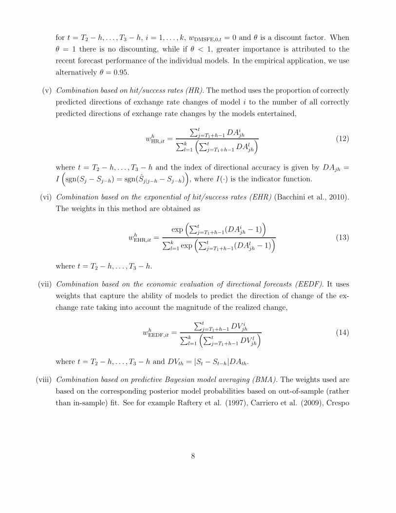
for t = T2 − h, . . . , T3 − h, i = 1, . . . , k, wDMSFE,0,t = 0 and θ is a discount factor. When
θ = 1 there is no discounting, while if θ < 1, greater importance is attributed to the
recent forecast performance of the individual models. In the empirical application, we use
alternatively θ = 0.95.
(v) Combination based on hit/success rates (HR). The method uses the proportion of correctly
predicted directions of exchange rate changes of model i to the number of all correctly
predicted directions of exchange rate changes by the models entertained,
whHR,it =
∑t
j=T1+h−1DAijh
∑k
l=1
(
∑t
j=T1+h−1DAljh
) (12)
where t = T2 − h, . . . , T3 − h and the index of directional accuracy is given by DAjh =
I(
sgn(Sj − Sj−h) = sgn(Sj|j−h − Sj−h))
, where I(·) is the indicator function.
(vi) Combination based on the exponential of hit/success rates (EHR) (Bacchini et al., 2010).
The weights in this method are obtained as
whEHR,it =
exp(
∑t
j=T1+h−1(DAijh − 1)
)
∑k
l=1 exp(
∑t
j=T1+h−1(DAljh − 1)
) (13)
where t = T2 − h, . . . , T3 − h.
(vii) Combination based on the economic evaluation of directional forecasts (EEDF). It uses
weights that capture the ability of models to predict the direction of change of the ex-
change rate taking into account the magnitude of the realized change,
whEEDF,it =
∑t
j=T1+h−1DVijh
∑k
l=1
(
∑t
j=T1+h−1DVljh
) (14)
where t = T2 − h, . . . , T3 − h and DVth = |St − St−h|DAth.
(viii) Combination based on predictive Bayesian model averaging (BMA). The weights used are
based on the corresponding posterior model probabilities based on out-of-sample (rather
than in-sample) fit. See for example Raftery et al. (1997), Carriero et al. (2009), Crespo
8
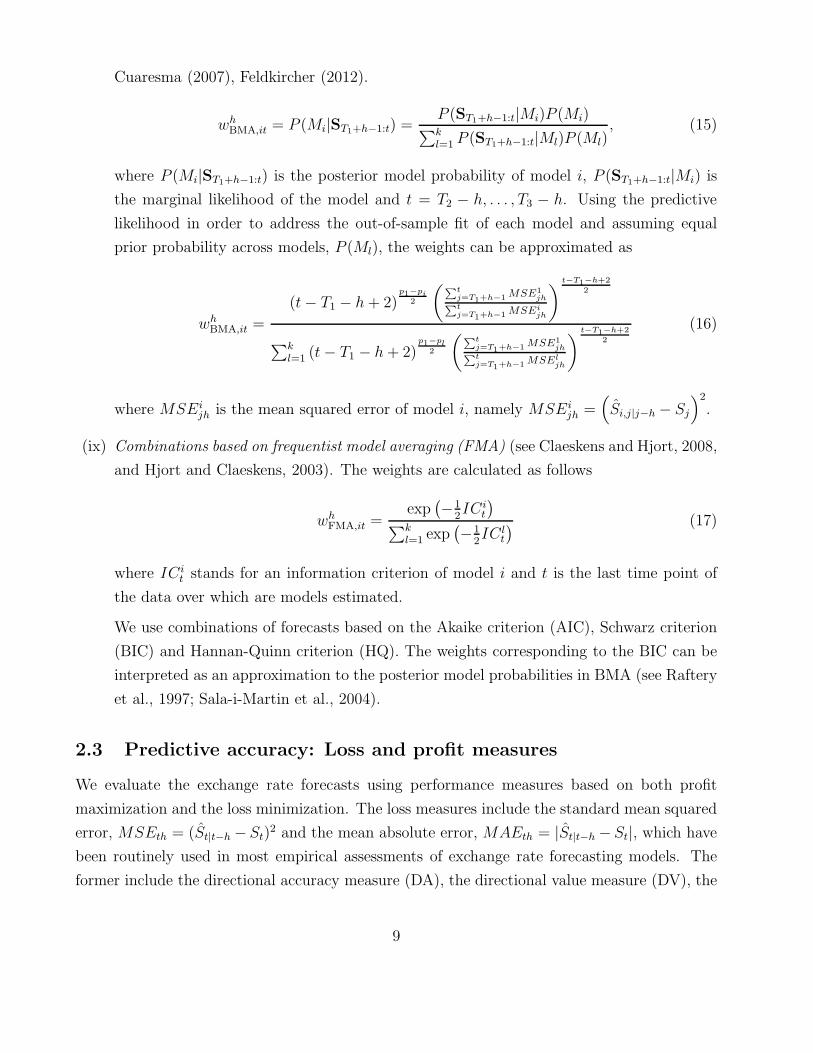
Cuaresma (2007), Feldkircher (2012).
whBMA,it = P (Mi|ST1+h−1:t) =
P (ST1+h−1:t|Mi)P (Mi)∑k
l=1 P (ST1+h−1:t|Ml)P (Ml), (15)
where P (Mi|ST1+h−1:t) is the posterior model probability of model i, P (ST1+h−1:t|Mi) is
the marginal likelihood of the model and t = T2 − h, . . . , T3 − h. Using the predictive
likelihood in order to address the out-of-sample fit of each model and assuming equal
prior probability across models, P (Ml), the weights can be approximated as
whBMA,it =
(t− T1 − h+ 2)p1−pi
2
(∑tj=T1+h−1 MSE1
jh∑t
j=T1+h−1 MSEijh
)
t−T1−h+2
2
∑k
l=1 (t− T1 − h+ 2)p1−pl
2
(∑tj=T1+h−1 MSE1
jh∑t
j=T1+h−1 MSEljh
)
t−T1−h+22
(16)
where MSEijh is the mean squared error of model i, namely MSEi
jh =(
Si,j|j−h − Sj
)2
.
(ix) Combinations based on frequentist model averaging (FMA) (see Claeskens and Hjort, 2008,
and Hjort and Claeskens, 2003). The weights are calculated as follows
whFMA,it =
exp(
−12IC i
t
)
∑k
l=1 exp(
−12IC l
t
) (17)
where IC it stands for an information criterion of model i and t is the last time point of
the data over which are models estimated.
We use combinations of forecasts based on the Akaike criterion (AIC), Schwarz criterion
(BIC) and Hannan-Quinn criterion (HQ). The weights corresponding to the BIC can be
interpreted as an approximation to the posterior model probabilities in BMA (see Raftery
et al., 1997; Sala-i-Martin et al., 2004).
2.3 Predictive accuracy: Loss and profit measures
We evaluate the exchange rate forecasts using performance measures based on both profit
maximization and the loss minimization. The loss measures include the standard mean squared
error, MSEth = (St|t−h − St)2 and the mean absolute error, MAEth = |St|t−h − St|, which have
been routinely used in most empirical assessments of exchange rate forecasting models. The
former include the directional accuracy measure (DA), the directional value measure (DV), the
9

annualized returns from two different trading strategies generated by our forecasts and risk
adjusted performance measures given by the Sharpe ratios for both of the trading strategies.
The directional accuracy measure DAth = I(
sgn(St − St−h) = sgn(St|t−h − St−h))
, intro-
duced already above, is a binary variable indicating whether the direction of the exchange rate
change was correctly forecast at horizon h (DAth = 1) or not (DAth = 0). While the function
DAth is robust to outlying forecasts, it does not consider the size of the realized directional
movements. The economic value of directional forecasts is better captured by assigning to each
correctly predicted change its magnitude (see Blaskowitz and Herwartz, 2011). The directional
value (DV ) statistic, defined as DVth = |St − St−h|DAth is used for this purpose.
The performance of exchange rate forecasts based on their profitability is evaluated by
constructing simple trading strategies based on the predictions. We start with a simple trading
strategy as described in Gencay (1998), where the selling/buying signal is based on the current
exchange rate, namely, forecast upward movements of the exchange rate with respect to the
actual value (positive returns) are executed as long positions while the forecast downward
movements (negative returns) are executed as short positions; i.e., the total return of the
trading strategy over n periods is given by
RSh =
n∑
t=1
ySt−h,hrth =
n∑
t=1
RSth (18)
where rth = log(St/St−h), t = 1, . . . , n,
ySt−h,h =
−1, for selling signal (forecast downward movement for horizon h)
St|t−h < St−h
1, for buying signal (forecast upward movement for horizon h)
St|t−h > St−h
and RSth = ySt−h,hrth.We label this trading strategy TSS. While this trading strategy is based on
comparing current and predicted exchange rates, a comparison of the forecast with the forward
rate would be a natural building block for an alternative trading strategy. The trading strategy
used in Boothe (1983), for instance, generates signals based on the comparison of the forecast
value to the current forward rate
RFh =
n∑
t=1
yFt−h,hrth =
n∑
t=1
RFth (19)
10
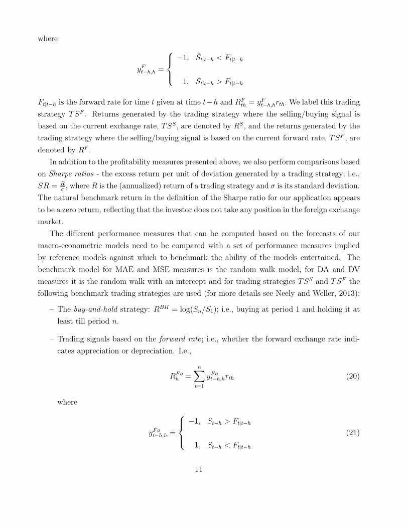
where
yFt−h,h =
−1, St|t−h < Ft|t−h
1, St|t−h > Ft|t−h
Ft|t−h is the forward rate for time t given at time t−h and RFth = yFt−h,hrth.We label this trading
strategy TSF . Returns generated by the trading strategy where the selling/buying signal is
based on the current exchange rate, TSS, are denoted by RS, and the returns generated by the
trading strategy where the selling/buying signal is based on the current forward rate, TSF , are
denoted by RF .
In addition to the profitability measures presented above, we also perform comparisons based
on Sharpe ratios - the excess return per unit of deviation generated by a trading strategy; i.e.,
SR = Rσ, where R is the (annualized) return of a trading strategy and σ is its standard deviation.
The natural benchmark return in the definition of the Sharpe ratio for our application appears
to be a zero return, reflecting that the investor does not take any position in the foreign exchange
market.
The different performance measures that can be computed based on the forecasts of our
macro-econometric models need to be compared with a set of performance measures implied
by reference models against which to benchmark the ability of the models entertained. The
benchmark model for MAE and MSE measures is the random walk model, for DA and DV
measures it is the random walk with an intercept and for trading strategies TSS and TSF the
following benchmark trading strategies are used (for more details see Neely and Weller, 2013):
– The buy-and-hold strategy: RBH = log(Sn/S1); i.e., buying at period 1 and holding it at
least till period n.
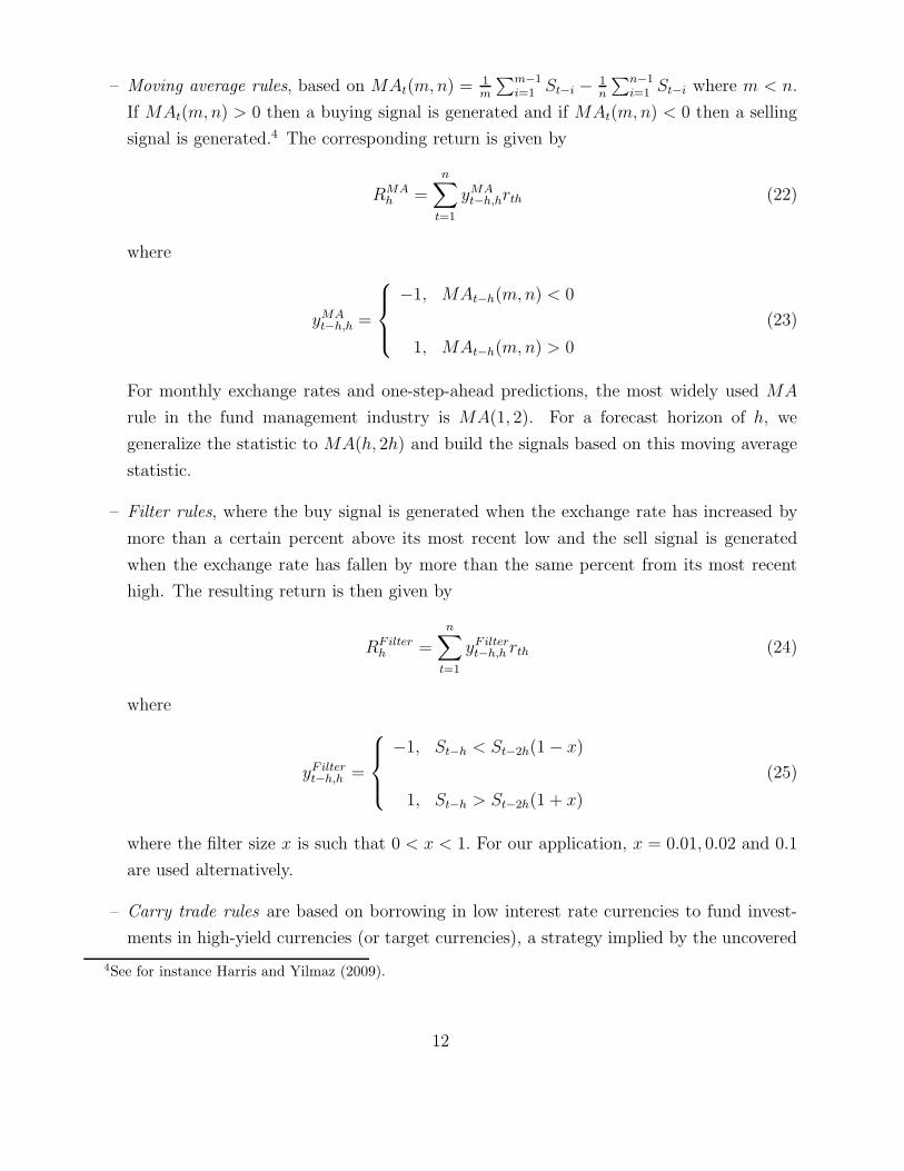
– Trading signals based on the forward rate; i.e., whether the forward exchange rate indi-
cates appreciation or depreciation. I.e.,
RFoh =
n∑
t=1
yFot−h,hrth (20)
where
yFot−h,h =
−1, St−h > Ft|t−h
1, St−h < Ft|t−h
(21)
11
– Moving average rules, based on MAt(m,n) =1m
∑m−1i=1 St−i − 1
n
∑n−1i=1 St−i where m < n.
If MAt(m,n) > 0 then a buying signal is generated and if MAt(m,n) < 0 then a selling
signal is generated.4 The corresponding return is given by
RMAh =
n∑
t=1
yMAt−h,hrth (22)
where
yMAt−h,h =
−1, MAt−h(m,n) < 0
1, MAt−h(m,n) > 0
(23)
For monthly exchange rates and one-step-ahead predictions, the most widely used MA
rule in the fund management industry is MA(1, 2). For a forecast horizon of h, we
generalize the statistic to MA(h, 2h) and build the signals based on this moving average
statistic.
– Filter rules, where the buy signal is generated when the exchange rate has increased by
more than a certain percent above its most recent low and the sell signal is generated
when the exchange rate has fallen by more than the same percent from its most recent
high. The resulting return is then given by
RF ilterh =
n∑
t=1
yF iltert−h,h rth (24)
where
yF iltert−h,h =
−1, St−h < St−2h(1− x)
1, St−h > St−2h(1 + x)
(25)
where the filter size x is such that 0 < x < 1. For our application, x = 0.01, 0.02 and 0.1
are used alternatively.
– Carry trade rules are based on borrowing in low interest rate currencies to fund invest-
ments in high-yield currencies (or target currencies), a strategy implied by the uncovered
4See for instance Harris and Yilmaz (2009).
12

interest rate parity (see Ilut, 2012).5 The resulting return is given by
RCTh =
n∑
t=1
yCTt−h,hrth (26)
where
yCTt−h,h =
−1, idt−h,h < ift−h,h
1, idt−h,h > ift−h,h
where idt−h,h is a domestic interest rate for h−steps ahead while ift−h,h is a foreign interest
rate for h−steps ahead.
3 Estimation, prediction and testing for data snooping
3.1 Estimation details
We base our comparison on monthly data spanning the period from January 1980 until De-
cember 2013 for the EUR/USD, EUR/GBP, EUR/CHF and EUR/JPY exchange rates. The
beginning of the sample is thus T0 = January 1980, the beginning of the hold-out forecasting
sample for individual models used in order to obtain weights based on predictive accuracy is
given by T1 = January 2007. The beginning of the actual out-of-sample forecasting sample is
T2 = January 2010, and the end of the data sample is T3 = December 2013.6
The lag length of the VAR, VEC and DVAR specifications is selected using the AIC criterion
for potential lag lengths ranging from 1 to 12 lags.7 For the VEC models, selection of the lag
length and the number of cointegration relationships is carried out simultaneously using the
AIC. Since VAR models are known to forecast poorly due to overfitting (see, e.g., Fair, 1979), we
also estimate subset-VAR specifications, where individual parameters of the VAR specification
are set equal to zero recursively using t-tests (see Kunst and Neusser, 1986, for a similar
approach). While in the set of restricted specifications based on the monetary model which are
mentioned in section 2 the parameters are constrained based on theoretical assumptions, in the
case of subset-VARs the corresponding specification is estimated and insignificant lags of the
5Bekaert et al. (2007) and Krishnakumar and Neto (2012) point out the importance of the link between theinterest rate parity and the hypothesis of the term structure for the determination of the exchange rate.
6The sources for all variables used are given in the data appendix.7Our results are however robust to model selection using BIC or the HQ criterion.
13
endogenous variables are removed from the model specification. The restrictions are imposed
by setting to zero those parameters for which we cannot reject that they are equal to zero using
a one-sided t-test.
In addition to standard VAR, DVAR and VEC models, we also estimate Bayesian VARs.
The standard Bayesian approach for estimating VAR models was mainly developed by Doan et
al. (1984) and Litterman (1986), who suggest that assuming as a prior that the variables in the
VAR follow a random walk would be sensible for economic variables (the Litterman/Minessota
prior). In the case of exchange rates, it would furthermore be consistent with the efficient
market hypothesis. We thus estimate DVAR specifications using Bayesian methods, setting the
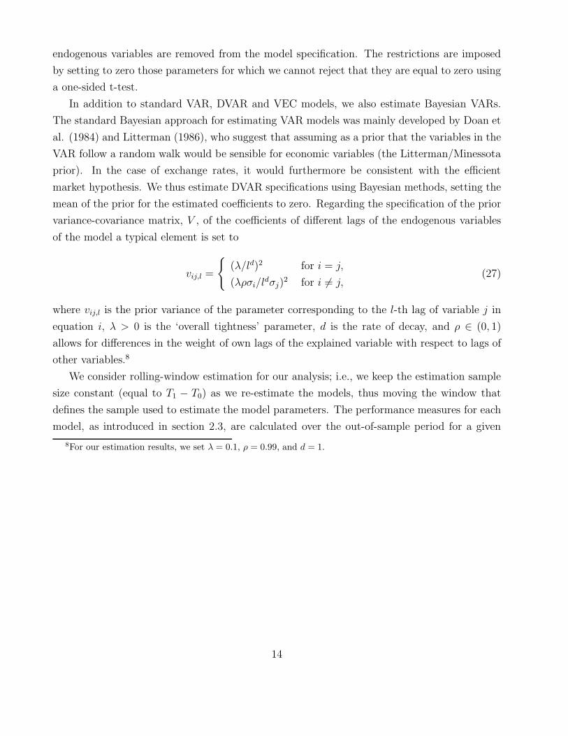
mean of the prior for the estimated coefficients to zero. Regarding the specification of the prior
variance-covariance matrix, V , of the coefficients of different lags of the endogenous variables
of the model a typical element is set to
vij,l =
{
(λ/ld)2 for i = j,
(λρσi/ldσj)
2 for i 6= j,(27)
where vij,l is the prior variance of the parameter corresponding to the l-th lag of variable j in
equation i, λ > 0 is the ‘overall tightness’ parameter, d is the rate of decay, and ρ ∈ (0, 1)
allows for differences in the weight of own lags of the explained variable with respect to lags of
other variables.8
We consider rolling-window estimation for our analysis; i.e., we keep the estimation sample
size constant (equal to T1 − T0) as we re-estimate the models, thus moving the window that
defines the sample used to estimate the model parameters. The performance measures for each
model, as introduced in section 2.3, are calculated over the out-of-sample period for a given
8For our estimation results, we set λ = 0.1, ρ = 0.99, and d = 1.
14

forecasting horizon and aggregated as follows
MSEh =
T3−T2∑
j=0
MSET2+j,h
MAEh =
T3−T2∑
j=0
MAET2+j,h
DAh =
T3−T2∑
j=0
DAT2+j,h
T3 − T2 + 1
DVh =
∑T3−T2
j=0 DVT2+j,h∑T3−T2
j=0 |ST2+j − ST2+j−h|
=
∑T3−T2
j=0 |ST2+j − ST2+j−h|DAT2+j,h∑T3−T2
j=0 |ST2+j − ST2+j−h|
where h = 1, . . . , 12.
3.2 Data snooping bias free tests for equal predictive ability
In order to assess whether the predictive superiority of certain models is systematic and not due
to luck, we also perform bootstrap tests for the comparison of predictive ability with respect to
the benchmark models and trading strategies. In particular, we use the ‘reality check’ (RC) test
by White (2000), the test for superior predictive ability (SPA) by Hansen (2005), the stepwise
test of multiple check (stepM-RC) by Romano and Wolf (2005) and the stepwise multiple
superior predictive ability test (stepM-SPA) by Hsu et al. (2010).
The following relative performance measures, dith, i = 1, . . . , k, t = T2, T2 + 1, . . . , T3,
h = 1, . . . , 12 are computed and the tests are defined based on them:
dith =
MSERW,th − MSEith
MAERW,th − MAEith
DAith − DARWint,th
DVith − DVRWint,th
ySithrth − yref,thrth
yFithrth − yref,thrth
SRSith − SRref
ith
SRFith − SRref
ith
(28)
15
Index ref denotes the reference/benchmark trading rule, implying that we concentrate on
relative returns. The benchmark trading strategies are defined by (20)–(27). Thus, ref ∈{Fo,MA, F ilter, CT}. SRS stands for the Sharpe ratio implied by the trading strategy TSS
as defined in (18), SRF stands for the Sharpe ratio implied by the trading strategy TSF as
defined in (19)9 and RWint stands for the random walk with an intercept.
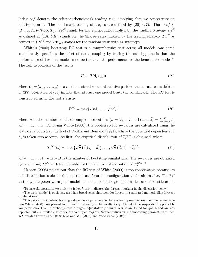
White’s (2000) bootstrap RC test is a comprehensive test across all models considered
and directly quantifies the effect of data snooping by testing the null hypothesis that the
performance of the best model is no better than the performance of the benchmark model.10
The null hypothesis of the test is
H0 : E(dt) ≤ 0 (29)
where dt = (d1t, . . . , dkt) is a k−dimensional vector of relative performance measures as defined
in (28). Rejection of (29) implies that at least one model beats the benchmark. The RC test is
constructed using the test statistic
TRCn = max{
√nd1, . . . ,
√ndk} (30)
where n is the number of out-of-sample observations (n = T3 − T2 + 1) and di =∑T3
t=T2dit
for i = 1, . . . , k. Following White (2000), the bootstrap RC p−values are calculated using the
stationary bootstrap method of Politis and Romano (1994), where the potential dependence in
dt is taken into account. At first, the empirical distribution of TRC∗
n is obtained, where
TRC∗n (b) = max
{√n(
d1(b)− d1)
, . . . ,√n(
dk(b)− dk)}
(31)
for b = 1, . . . , B, where B is the number of bootstrap simulations. The p−values are obtained
by comparing TRCn with the quantiles of the empirical distribution of TRC∗
n .11
Hansen (2005) points out that the RC test of White (2000) is too conservative because its
null distribution is obtained under the least favorable configuration to the alternative. The RC
test may lose power when poor models are included in the group of models under consideration.
9To ease the notation, we omit the index h that indicates the forecast horizon in the discussion below.10The term ‘model’ is obviously used in a broad sense that includes forecasting rules and methods (like forecast
combinations).11This procedure involves choosing a dependence parameter q that serves to preserve possible time dependence
(see White, 2000). We present in our empirical analysis the results for q=0.9, which corresponds to a plausiblylow persistence level in exchange rate changes. Qualitatively similar results are found for q=0.5 and are notreported but are available from the authors upon request. Similar values for the smoothing parameter are usedin Gonzalez-Rivera et al. (2004), Qi and Wu (2006) and Yang et al. (2008).
16

To improve the power of the test, Hansen (2005) proposes the superior predictive ability (SPA)
test. The null hypothesis of the SPA test is the same as in the in White’s RC test, but Hansen
(2005) uses the studentized test statistic to improve the power.12 The test statistic for the SPA
test is
T SPAn = max
[
max
{√nd1s1
, . . . ,
√ndksk
}
, 0
]
(32)
where si is a consistent estimator of var(√ndi), i = 1, . . . , k. The same bootstrap method of
Politis and Romano (1994) is used to calculate the empirical distribution of the statistic under
the null.
One drawback of both RC and SPA tests is that they do not aim at explicitly identifying
the models which outperforms the benchmark. Romano and Wolf (2005) propose the stepM-
RC test that can identify also those models for which E(dit) > 0 holds. For a given model i,
(i = 1, . . .) the following individual testing problems are considered
H i0 : E(dit ≤ 0) vs H i
A : E(dit > 0) (33)
This multiple testing method yields a decision for each individual testing problem (by either
rejecting H i0 or not). The individual decisions are made such that the familywise error rate13
is asymptotically achieved at the significance level α which is achieved by constructing a joint
confidence region with a nominal joint coverage probability of 1 − α. This stepwise procedure
is implemented as follows. Without loss of generality we assume that {di}ki=1 are arranged in
a descending order. Top j1 null hypotheses are rejected (i.e., top j1 models outperform the
benchmark) if√ndl, l = 1, . . . , j1 is greater than the bootstrapped critical value computed
from the bootstrap procedure as in the RC test. If none of the null hypotheses is rejected, the
procedure terminates. Otherwise, d1t, . . . , dj1t, t = T2, . . . , T3 are removed from the data and
the bootstrap simulation is applied to the rest of the data to obtain the new critical value. If√ndl, l = 1, . . . , j2 is greater than the new bootstrapped critical value then the following j2 null
hypotheses are rejected. The procedure continues until no more null hypotheses are rejected.
In our analysis we use significance levels of 5% and 10%.
Hsu et al. (2010) extend the SPA of Hansen (2005) to a stepwise SPA test in the way
Romano and Wolf (2005) did it for the RC test. They show analytically that the stepM-SPA
12The improvement of the power of the SPA test over the RC test is confirmed by simulations in Hansen(2005).
13The familywise error rate is defined as the probability of rejecting at least one true null hypothesis. Formore details, see Romano and Wolf (2005).
17

test is more powerful than stepM-RC test. The step wise procedure is the same as in the
stepM-RC test but with RC test statistics replaced by PCA test statistics.
4 Results
Table 1 presents the abbreviations of the models, forecast combination techniques and bench-
mark trading strategies used in the analysis. Tables 2 to 9 presents the results of the analysis
for each exchange rate, theoretical framework (monetary versus capital flows) and three dif-
ferent prediction horizons (one, six and twelve months ahead). The tables are structured in
three blocks, each one corresponding to a different forecasting horizon. Each block, in turn, is
divided into three different parts. The top part of the block presents the results for those indi-
vidual specifications which perform best according to the criteria described in section 2.2 and
section 2.3. In the central part of the block, we present the results for all forecast combination
methods used. The bottom part of each block, in turn, presents the corresponding measures
for the best-performing benchmark strategies. The forecasts are evaluated using the loss and
profit measures described in section 2.314 and the predictive superiority of the models which
perform better than the benchmark is assessed by means of the bootstrap stepM-SPA test by
Hsu et al. (2010).15
[Include Table 1 about here]
Tables 2 and 3 report the predictive ability measures of the monetary and capital flows
models as well as combinations thereof for the EUR/USD exchange rate. The random walk
model is always beaten by the best single individual model and the best combination of forecast
for 1-step and 6-steps ahead in terms of predictive ability as measured by MAE, MSE, DA and
DV (except for the best single individual model for MAE and MSE and 6-steps ahead). The
results are slightly different for measures based on 12-steps ahead forecasts. Here, the random
walk prevails over the other models for MAE and MSE. However, according to the stepM-SPA
test, only the differences in forecasting ability in terms of DA and DV appear significant, while
those measured by MAE and MSE measures are all insignificant. More specifically, we find for
DA and DV measures that their benchmark random walk model is systematically beaten by
the combination of forecasts based on the principal components for 6-steps and 12-steps ahead,
which appears superior at the 5% significance level using the stepM-SPA test. Furthermore,
14The loss measures are based on currency units. Note that returns generated by trading strategies arecalculated from the position of a foreign investor.
15We used all the tests described in section 3.2, but report only the results for the stepM-SPA test in thetables. Detailed results using the other tests are available from the authors upon request.
18

some capital flows models perform significantly better than the random walk for 1-step ahead
in terms of the DA and DV measures. Comparable results for directional forecast are found in
Yang et al. (2008) and Dal Bianco et al. (2012). In particular, Yang et al. (2008) point at
the forecast superiority of alternative specifications when using weekly data, whereas only one
model significantly outperforms the random walk when using daily data. Using weekly data,
Dal Bianco et al. (2012), who propose a fundamentals-based econometric model for the weekly
changes in the EUR/USD rate with the distinctive feature of mixing economic variables quoted
at different frequencies, find that their model significantly outperforms the random walk model
for long horizons.
[Include Tables 2 & 3 about here]
As for the performance of trading strategies based on the exchange rate forecasts, the results
show that only the returns from trading strategy TSF implied by the principal components
based forecasts combination method is significantly better than the best benchmark models
at a 10% significance level. This occurs for 6-steps and 12-steps ahead in the case of the
monetary model (see Table 2) and only for 6-steps ahead for the capital flows model. Looking
at the Sharpe ratios of returns generated by trading strategies TSS and TSF , a slightly stronger
evidence of risk adjusted profitability is found (in some cases the results are significant at 5%
level). More specifically, forecasts based on principal components are significantly better than
the benchmark models, carry trade and MA(12,24), for 6-steps and 12-steps ahead for both
the monetary and capital flows models. However, the Sharpe ratio takes values lower than
unity, and it has been argued that market practitioners in the foreign exchange market may
be not interested in a currency investment strategy that yields a Sharpe ratio less than unity
(see Sarno et al., 2006). It should be however noticed that the difference in performance of the
other alternative forecasting models with respect to the benchmark model is insignificant.
[Include Tables 4 & 5 about here]
Tables 4 and 5 depict the results for the forecasts of the EUR/GBP exchange rate. These
show that several individual forecasting models and combinations of forecast outperform the
random walk for DA and DV measures in 1-step and 12-steps ahead predictions, whereas results
turn to be all insignificant for MAE and MSE measures. In particular, we find that the forecast
combination based on OLS method and principal components outperform the random walk for
1-step ahead at 5% and 10% level, depending on the directional forecast measure considered
(see Tables 4 and 5), and three individual models (r-VAR, s-VAR and rs-VAR) along with
19

the forecast combination based on principal components yield the best performance for 12-
steps ahead. For 6-steps ahead, findings show no significant forecast superiority beyond the
benchmark specifications. On the whole, these findings contrast with those in Yang et al. (2008)
who report evidence of no significant predictability in terms of average directional accuracy for
all the forecasting models. As for the trading strategies, results reveal no systematic significant
superiority of the models and combinations entertained except for the forecast combinations
based on principal components and BMA for 6-steps ahead in the theoretical context of the
monetary model for both profit and risk adjusted profit measures generated by the trading
strategy TSF . Quantitatively, the combination of forecast based on principal components yields
the best performance. The benchmark model, based on the forward rate, achieves negative
returns. By and large, the results for the EUR/USD exchange rate are slightly better in terms
of profitability than those for the EUR/GBP, but low values for the Sharpe ratio do not trigger
much confidence in obtaining successful investments for potential investors.
[Include Tables 6 & 7 about here]
Tables 6 and 7 contain the results based on forecasts of the EUR/CHF exchange rate.
The findings show that none of the models and combinations used outperform the benchmark
(random walk) model for 1-step and 6-steps ahead for MAE and MSE measures. Surprisingly,
forecasts from some individual forecasting models (DVAR, s-DVAR,r-DVAR and BDVAR) and
two combinations of forecast (NEHSR and BMA) outperform the random walk for 12-steps
ahead for MAE and MSE measures. As for the predictability measured by the DA and DV
criteria, none of the forecasting methods is significantly superior to the benchmark model.
These results can be consistent with the heavy interventions of the Swiss central bank in the
foreign exchange market documented during the crisis (see e.g. Bordo et al., 2012), which are
likely to have affected the information content of macroeconomic fundamentals as a leading
indicator of exchange rate changes. The forecast ability of specifications and combinations for
both the monetary and the capital flows models is not significantly better than the benchmarks
when looking at returns implied by trading strategies TSS and TSF and their Sharpe ratios.
[Include Tables 8 & 9 about here]
The results of the prediction exercise for the EUR/JPY exchange rate, as reported in Tables
8 and 9, are marked by the widespread lack of evidence of statistical superiority against the
benchmark strategies. Only for the 1-step ahead in the case of DA and DV do we find a
general improvement through the use of econometric specifications based on the monetary
20

model. These results are in line with those in Yang et al. (2008) and emphasize the difficulty
of building successful trading strategies based on EUR/JPY predictions. In spite of the large
improvements in directional forecasts obtained through the use of econometric specifications
and combinations of forecasts in the short run (see for example the results presented in Table
8 for the 1-step ahead horizon), these do not translate to a significant superiority in terms
of Sharpe ratios, where strategies based on random walk predictions, carry trade or moving
averages are not systematically outperformed by the set of entertained specifications. As in
the case of the results for EUR/CHF, the frequency and size of the foreign exchange market
interventions of the monetary policy authority in Japan (see e.g. Chortareas et al., 2013) are
likely to play an important role in terms of affecting the predictive content of macroeconomic
fundamentals for the exchange rate.
Summing up the results across exchange rates and theoretical settings, several general con-
clusions can be drawn. First of all, there is no evidence of a “one size fits all” approach to
the specification of single multivariate time series models for exchange rate forecasting which
leads to systematically good predictive ability in terms of trading strategies. The use of error
correction specifications or Bayesian VAR models does not ensure a lower loss or a higher profit,
and there is no systematic relationship between the use of variables related to a particular the-
oretical setting (monetary or capital flows) and improvements in the predictive ability of the
model as measured by our loss and profit measures.
As compared to individual specifications and benchmark strategies, the use of forecast com-
bination methods tends to lead to improvements in the performance of trading rules implied by
our forecasts. In particular, forecast pooling based on principal components methods appears
to be the most robust technique for the EUR/USD and EUR/GBP. On the other hand, the
forecasts for the EUR/CHF exchange rate based on both individual models and forecast combi-
nations (namely the Bayesian model averaging method) do outperform the random walk model
for a long-term prediction horizon. As for the EUR/JPY exchange rate, the performance of
the forecasts obtained with macroeconometric models and their combinations does not robustly
improve over the standard benchmarks. This result supports the view that predicting exchange
rates using macroeconomic variables is a particularly difficult task in foreign exchange markets
where monetary policy interventions are frequent and sizeable. Such a result is in line, for
instance, with the work of Beine et al. (2007), Neely (2008) or Miyajima (2013), who find that
interventions increase the volatility of exchange rates and exchange rate forecasts.
In spite of the improvements in profit measures obtained by combinations of predictions for
EUR/USD and EUR/GBP, the results concerning differences in Sharpe ratios of returns given
by the trading strategies indicate that the margin for achieving systematic monetary profits
21
in the foreign exchange market using macroeconometric models is very limited and that the
answer to the question posed by the title of this paper is very likely to be “Unfortunately, no”.
5 Conclusions
Using a large battery of multivariate time series models and forecast combination methods, we
provide a systematic comparison of out-of-sample forecast accuracy in terms of loss and profit
measures for the EUR/USD, EUR/GBP, EUR/CHF and EUR/JPY exchange rates. The contri-
butions of this study are twofold. First, we use recently developed directional forecast accuracy
measures that account for both the direction and the size of the changes in exchange rates and
are robust to outliers. These measures provide an economically interpretable loss/success func-
tional framework in a decision-theoretical context. Second, we exploit the potential of a large
number of forecast combination methods for both forecast accuracy evaluation and profitability.
In doing so, we propose a new method of forecast combination based on the economic evaluation
of directional predictions. Our empirical results emphasize the lack of superiority of a single
specification or forecast combination technique over different prediction horizons and exchange
rates. The results for EUR/USD and the EUR/GBP, forecast combinations based on principal
component decompositions of individual model predictions appear particularly promising in im-
proving profitability based performance, albeit not systematically superior to the benchmarks
across forecasting horizons. The forecasts for the EUR/CHF exchange rate based on both in-
dividual models and forecast combinations outperform the random walk model for a long-term
prediction horizon. Finally, for the EUR/JPY exchange rate the results are not supportive of
any of the methods entertained and highlight the superiority of simple trading rules in terms
of profitability.
Future research will extend this study by considering optimal currency portfolios based on
a variety of foreign exchange trading strategies and their impact on different (risk adjusted)
profit measures. It will investigate whether the portfolios based on the trading strategies implied
by the exchange rate forecasts may have better performance than the portfolios based on the
technical trading rules strategies which do not use forecasts. As for the forecasts of the exchange
rate, both individual models and combinations of the forecasts will be used.
22
References
[1] R.Z. Aliber. 2000. Capital Flows, Exchange Rates, and the New International Financial
Architecture: Six Financial Crises in Search of a Generic Explanation. Open Economies
Review, 11, 43-61.
[2] F. Bacchini, A. Ciammola, R. Iannaccone, M. Marini. 2010. Combining forecasts for a flash
estimate of Euro area GDP. Contributi ISTAT, No. 3.
[3] A. Bailey, S. Millard, S. Wells. 2001. Capital flows and exchange rates. Bank of England
Quarterly Bulletin, Autumn, 310-318.
[4] G. Bekaert, R. Campbell, R. Harvey, C. Lundblad. 2007. Liquidity and expected returns:
Lessons from emerging markets. Review of Financial Studies, 20, 1783-1831.
[5] M. Beine, A. Benassy-Quere, R. MacDonald. 2007. The impact of central bank interven-
tion on exchange-rate forecast heterogeneity. Journal of the Japanese and International
Economies, 21, 38-63.
[6] C. Bergmeir, M. Costantini, J.M. Benıtez. 2014. On the usefulness of cross validation for
directional forecast evaluation. Computational Statistics and Data Analysis, forthcoming.
[7] J. Berkowitz, L. Giorgianni. 2001. Long-horizon exchange rate predictability? Review of
Economics and Statistics, 83, 81-91.
[8] O. Blaskowitz, H. Herwartz. 2009. Adaptive forecasting of the EURIBOR swap term struc-
ture. Journal of Forecasting, 28, 575-594.
[9] O. Blaskowitz, H. Herwartz. 2011. On economic evaluation of directional forecasts. Inter-
national Journal of Forecasting, 27, 1058-1065.f
[10] P. Boothe. 1983. Speculative profit opportunities in the canadian foreign exchange market,
1974-78. The Canadian Journal of Economics, 16, 603-611.
[11] M.D. Bordo, O.F. Humpage, A.J. Schwartz. 2012. Epilogue: Foreign Exchange Market
Operations in the Twentieth Century. NBER Working Paper 17984.
[12] J. Boudoukh, M. Richardson, R.F. Whitelaw. 2008. The myth of long-horizon predictabil-
ity. Review of Financial Studies, 21, 1577-1605.
23

[13] A. Carriero, G. Kapetanios, M. Marcellino. 2009. Forecasting exchange rates with a large
Bayesian VAR. International Journal of Forecasting, 25, 400-417.
[14] G. Claeskens, N.L. Hjort. 2008. Model Selection and Model Averaging. Cambridge: Cam-
bridge University Press.
[15] Y.W. Cheung, M.D. Chinn, A.G. Pascual. 2005. Empirical exchange rate models of the
nineties: Are any fit to survive? Journal of International Money and Finance, 24, 1150-
1175.
[16] M.D. Chinn, R.A. Meese. 1995. Banking on currency forecasts: How predictable is change
in money? Journal of International Economics, 38, 161-178.
[17] G. Chortareas, Y. Jiang, J.C. Nankervis. 2013. Volatility and Spillover Effects of Yen
Interventions. Review of International Economics, 21, 671-689.
[18] M. Costantini, C. Pappalardo. 2010. A hierarchical procedure for the combination of fore-
casts. International Journal of Forecasting, 26, 725-743.
[19] J. Crespo Cuaresma. 2007. Forecasting euro exchange rates: How much does model aver-
aging help? Working paper of University of Innsbruck, 2007-24.
[20] M. Dal Bianco, M. Camacho, G.P. Quiros. 2012. Short-run forecasting of the euro-dollar
exchange rate with economic fundamental. Journal of International Money and Finance,
31, 377-396.
[21] T. Doan, R. Litterman, C. Sims. 1984. Forecasting and conditional projections using realist
prior distributions. Econometric Review, 3, 1-100.
[22] R. Dornbusch. 1976. Expectations and exchange rate dynamics. Journal of Political Econ-
omy, 84, 1161-1176.
[23] R. Fair. 1979. An analysis of the accuracy of four macroeconometric models. Journal of
Political Economy, 87, 701-18.
[24] M. Feldkircher. 2012. Forecast combination and Bayesian model averaging: A prior sensi-
tivity analysis. Journal of Forecasting, 31, 361-376.
[25] J.A. Frenkel. 1976. A monetary approach to the exchange rate: Doctrinal aspects and
empirical evidence. Scandinavian Journal of Economics, 78, 200-224.
24

[26] R. Gencay. 1998. The predictability of security returns with simple technical trading rules.
Journal of Empirical Finance, 5, 347-359.
[27] G. Gonzalez-Rivera, T.H. Lee, S. Mishra. 2004. Forecasting volatility: A reality check based
on option pricing, utility function, value-at-risk, and predictive likelihood. International
Journal of forecasting, 20, 629-645.
[28] C.W.J. Granger, R. Ramanathan. 1984. Improved methods of combining forecasts. Journal
of Forecasting, 3, 197-204.
[29] P.R. Hansen. 2005. A test for superior predictive ability. Journal of Business and Economic
Statistics, 23, 365380.
[30] R.D.F. Harris, F. Yilmaz. 2009. A momentum trading strategy based on the low frequency
component of the exchange rate. Journal of Banking and Finance, 33, 1575-1585.
[31] N.L. Hjort, G. Claeskens. 2003. Frequentist model average estimators. Journal of American
Statistical Association, 98, 879-899.
[32] J. Hlouskova, M. Wagner. 2013. The determinants of long-run economic growth: A concep-
tually and computationally simple approach. Swiss Journal of Economics and Statistics,
149, 445-492.
[33] Y. Hong and T.H. Lee. 2003. Inference on predictability of foreign exchange rate changes via
generalized spectrum and nonlinear time series models. Review of Economics and Statistics,
85, 1048-1062.
[34] P. Hooper, J. Morton. 1982. Fluctuations in the dollar: A model of nominal and real
exchange rate determination. Journal of International Money and Finance, 1, 39-56.
[35] N.P. Hsu, Y. Hsu, C. Kuan. 2010. Testing the predictive ability of technical analysis using
a new stepwise test without data snooping bias. Journal of Empirical Finance, 17, 471-484.
[36] C. Ilut. 2012. Ambiguity aversion: Implications for the uncovered interest rate parity
puzzle. American Economic Journal: Macroeconomics, 4, 33-65.
[37] J. James, I. Marsh, L. Sarno. 2012. Handbook of Exchange Rates. John Wiley & Sons Inc.
[38] L. Kilian. 1999. Exchange rates and monetary fundamentals: What do we learn from
long-horizon regressions? Journal of Applied Econometrics, 14, 491-510.
25

[39] J. Krishnakumar and D. Neto. 2012. Testing uncovered interest rate parity and term struc-
ture using a three-regime threshold unit root VECM: An application to the swiss isle of
interest rates. Oxford Bulletin of Economics and Statistics, 74, 180-202.
[40] R.M. Kunst and K. Neusser. 1986. A forecasting comparison of some VAR techniques.
International Journal of Forecasting, 2, 447-456.
[41] R.B. Litterman. 1986. Forecasting with Bayesian vector autoregressions. Five years of
experience. Journal of Business and Economic Statistics, 4, 25-38.
[42] R. MacDonald, M.P. Taylor. 1994. The monetary model of the exchange rate: Long-run
relationships, short-run dynamics and how to beat a random walk. Journal of International
Money and Finance, 13, 276-290.
[43] N.C. Mark. 1995. Exchange rates and fundamentals: evidence on long-horizon prediction.
American Economic Review, 85, 201-218.
[44] N.C. Mark, D. Sul. 2001. Nominal exchange rates and monetary fundamentals: Evidence
from a small post-Bretton Woods panel. Journal of International Economics, 53, 29-52.
[45] R.A. Meese, K.S. Rogoff. 1983. Empirical exchange rate models of the seventies. Do they
fit out of sample? Journal of International Economics, 14, 3-24.
[46] L. Menkhoff, M.P. Taylor. 2007. The obstinate passion of foreign exchange professionals:
Technical analysis. Journal of Economic Literature, 45, 936-972.
[47] K. Miyajima, 2013. Foreign exchange intervention and expectation in emerging economies.
BIS Working Papers 414, Bank for International Settlements.
[48] C.J. Neely. 2008. Central bank authorities’ beliefs about foreign exchange intervention.
Journal of International Money and Finance, 27, 1-25.
[49] C.J. Neely, P.A. Weller. 2013. Lessons from the evolution of foreign exchange trading
strategies. Journal of Banking & Finance, 37, 3783-3798.
[50] D. Politis, J. Romano. 1994. The stationary bootstrap. Journal of the American Statistical
Association, 89, 1303-1313.
[51] M. Qi, Y. Wu. 2006. Technical trading-rule profitability, data snooping, and reality check:
Evidence from the foreign exchange market. Journal of Money Credit and Banking, 38,
2135-2158.
26
[52] A.E. Raftery, D. Madigan, J.A. Hoeting. 1997. Bayesian model averaging for regression
models. Journal of the American Statistical Association, 92, 179-191.
[53] J. Romano, M. Wolf. 2005. Stepwise multiple testing as formalized data snooping. Econo-
metrica, 73, 1237-1282.
[54] X. Sala-i-Martin, G. Doppelhofer, R.I. Miller. 2004. Determinants of long-term growth: A
Bayesian averaging of classical estimates (BACE) approach. American Economic Review,
94, 813-835.
[55] L. Sarno, G. Valente, H. Leon. 2006. Nonlinearity in deviations from uncovered interest
parity: An explanation of the forward bias puzzle. Review of Finance, 10, 443-482.
[56] J.H. Stock, M.W. Watson. 2004. Combination forecasts of output growth in a seven-country
data set. Journal of Forecasting, 23, 405-430.
[57] H. White. 2000. A reality check for data snooping. Econometrica, 68, 1097-1127.
[58] J. Yang, X. Su, J.W. Kolari. 2008. Do Euro exchange rates follow a martingale? Some
out-of-sample evidence? Journal of Banking and Finance, 32, 729-740.
27

Appendix: Data description and sources
All time series have monthly periodicity (January 1980 to December 2013), and have been
extracted from Thomson Financial Datastream. The variables used for EU-11, Japan, Switzer-
land, UK and USA, are:
• Money supply: M1 aggregate, indexed 1990:1=100. Seasonally unadjusted.
• Output: Industrial production index 1990:1=100.
• Short term interest rate: 3-month interbank offered rate.
• Long term interest rate: 10-year rate interest rate on government bonds
• leading indicator for Germany as a proxy for Europe: IFO index
• leading indicator for Japan: Leading diffusion index from Cabinet Office
• leading indicator for Switzerland: KOF economic barometer
• leading indicator for UK: CBI output volume index
• leading indicator for US: ISM index
• Stock market indices covering at least 80% of market capitalization in the respective
country.
28

Table 1: Models, combination methods and benchmarks
Abbreviations DescriptionIndividual models
VAR(p) Vector autoregression in levels based on domestic and foreign variables with p lagsDVAR(p) Vector autoregression in first differences based on domestic and foreign variables with p lagsVEC(c,p) Vector error correction model based on domestic and foreign variables with c cointegration relationshipsr-VAR(p) Restricted VAR, based on differences between domestic and foreign variablesr-DVAR(p) Restricted DVAR, based on differences between domestic and foreign variablesr-VEC(c,p) Restricted VEC, based on differences between domestic and foreign variables with c cointegration relationshipss-VAR(p) Subset vector autoregression in levels based on domestic and foreign variables with p lagss-DVAR(p) Subset vector autoregression in first differences based on domestic and foreign variables with p lagsrs-VAR(p) Restricted subset VAR, based on differences between domestic and foreign variablesrs-DVAR(p) Restricted subset DVAR, based on differences between domestic and foreign variablesBDVAR(p) Bayesian vector autoregression in first differences based on domestic and foreign variablesr-BDVAR(p) Bayesian vector autoregression in first differences based on differences between domestic and foreign variables
Forecast combination methodsmean Forecasting combination based on mean of individual predictionstmean Forecasting combination based on trimmed mean of individual predictionsmedian Forecasting combination based on median of individual predictionsOLS Forecasting combination based on pooling using OLSPC Forecasting combination based on principal componentsDMSFE Forecasting combination based on discounted mean square forecast errorsHR Forecasting combination based on hit ratesEHR Forecasting combination based on exponential of hit ratesEEDF Forecasting combination based on the economic evaluation of directional forecastsBMA Forecasting combination based on Bayesian model averaging weights using the predictive likelihoodFMA-aic Forecasting combination based on AIC weightsFMA-bic Forecasting combination based on BIC weightsFMA-hq Forecasting combination based on Hannan-Quinn weights
BenchmarksRW Random walk model (for MAE and MSE)RWint Random walk model with intercept (for DA and DV)BH Buy-and-hold trading strategy (for TSS and TSF )Forward rate Rule based on the forward rate (for TSS and TSF )MA(m, n) Rule based on differences between moving averages over m and n periods (for TSS and TSF )Filter Filter rule based trading strategy (for TSS and TSF )CT Carry trade rule (for TSS and TSF )
29

Table 2: Forecasts of the monetary model for the EUR/USD exchange rate
Model MAE MSE DA DV RS RF SRS SRF
1-stepr-VAR(12) 0.712 0.016 60.417 68.887 8.672 7.481 0.313 0.266rs-VAR(2) 0.678 0.015 60.417 67.735 8.046 4.755 0.288 0.166mean 0.712 0.016 54.167 62.856 5.751 3.801 0.202 0.132tmean 0.710 0.016 54.167 60.016 4.490 3.801 0.156 0.132median 0.690 0.015 58.333 63.627 6.066 4.755 0.213 0.166OLS 0.769 0.019 52.083 59.360 4.267 3.177 0.148 0.110PC 0.684 0.016 45.833 52.047 1.130 5.544 0.039 0.194DMSFE 0.706 0.016 54.167 60.016 4.490 3.801 0.156 0.132HR 0.712 0.016 54.167 62.856 5.751 3.801 0.202 0.132EHR 0.732 0.018 50.000 52.306 0.892 6.643 0.031 0.235EEDF 0.713 0.016 54.167 62.856 5.751 3.801 0.202 0.132BMA 0.793 0.021 47.917 54.906 2.056 6.643 0.071 0.235FMA-aic 0.755 0.019 45.833 47.117 -1.405 6.103 -0.048 0.215FMA-bic 0.716 0.017 58.333 67.405 7.771 3.243 0.278 0.112FMA-hq 0.733 0.017 52.083 61.683 5.195 3.801 0.182 0.132RW 0.686 0.016 47.917 46.675MA(1,2) 6.893 6.893 0.244 0.244
6-stepsr-VAR(12) 2.556 0.192 50.000 61.837 2.713 2.140 0.210 0.164r-VEC(2,11) 2.617 0.206 52.083 60.650 2.360 -0.136 0.182 -0.010s-DVAR(1) 1.955 0.122 45.833 42.485 -1.574 -1.156 -0.12 -0.088rs-VAR(2) 1.990 0.117 52.083 62.135 2.666 0.955 0.206 0.073mean 2.136 0.138 35.417 36.835 -2.796 -0.998 -0.217 -0.076tmean 2.119 0.137 37.500 39.890 -2.168 -1.072 -0.166 -0.081median 1.998 0.124 37.500 39.879 -2.191 -1.046 -0.168 -0.079OLS 2.822 0.255 43.750 45.732 -0.829 -1.403 -0.063 -0.107PC 1.896 0.109 72.917 80.388 6.601 7.024 0.579 0.631
DMSFE 2.103 0.134 33.333 36.727 -2.818 -1.095 -0.219 -0.083HR 2.168 0.142 41.667 46.645 -0.696 -0.998 -0.053 -0.076EHR 3.112 0.284 45.833 54.930 1.010 0.041 0.077 0.003EEDF 2.181 0.144 37.500 39.815 -2.184 -0.998 -0.168 -0.076BMA 2.743 0.224 41.667 45.052 -1.098 -1.481 -0.083 -0.113FMA-aic 2.398 0.177 47.917 53.282 0.689 0.009 0.052 0.001FMA-bic 2.033 0.131 45.833 46.471 -0.813 -0.628 -0.062 -0.048FMA-hq 2.174 0.150 43.750 43.262 -1.464 -0.845 -0.112 -0.064RW 1.916 0.113 50.000 41.065CT 4.116 4.116 0.328 0.328
12-stepsr-VAR(12) 3.660 0.433 50.000 64.691 1.943 1.133 0.254 0.145rs-VAR(2) 2.622 0.191 56.25 61.821 1.583 0.509 0.205 0.065r-BDVAR(4) 2.487 0.188 39.583 32.598 -2.311 -3.075 -0.306 -0.423mean 3.027 0.255 33.333 36.021 -1.820 -2.074 -0.237 -0.272tmean 2.951 0.240 35.417 38.385 -1.525 -1.84 -0.197 -0.239median 2.670 0.193 37.500 38.612 -1.522 -1.635 -0.196 -0.211OLS 9.012 6.963 52.083 58.318 1.098 1.107 0.140 0.141PC 2.414 0.172 72.917 83.300 4.379 4.406 0.669 0.674
DMSFE 3.061 0.259 33.333 36.021 -1.820 -2.498 -0.237 -0.333HR 3.139 0.275 33.333 36.021 -1.820 -2.369 -0.237 -0.314EHR 4.130 0.491 25.000 25.093 -3.250 -3.310 -0.452 -0.462EEDF 3.179 0.284 33.333 36.021 -1.820 -2.378 -0.237 -0.316BMA 3.737 0.443 37.500 41.591 -1.099 -1.629 -0.140 -0.211FMA-aic 3.408 0.355 39.583 44.390 -0.745 -1.347 -0.095 -0.173FMA-bic 2.805 0.224 41.667 38.670 -1.506 -2.340 -0.194 -0.310FMA-hq 3.129 0.284 41.667 44.201 -0.796 -1.551 -0.101 -0.200RW 2.330 0.163 43.750 41.265MA(12,14) 2.335 2.335 0.310 0.310
See Table 1 for the abbreviation of the models. Underlined bold figures indicate that the null hypothesis that
the model does not outperform the benchmark model is rejected at the 5% significance level and underlined
italic figures indicate that the null hypothesis is rejected at the 10% significance level using the stepM-SPA test.
The stepM-SPA test is performed setting the dependence parameter q equal to 0.9 and the number of bootstrap
simulations is equal to 5000. Both MAE and MSE loss measures are reported in exchange rate levels.
30
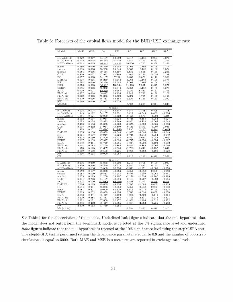
Table 3: Forecasts of the capital flows model for the EUR/USD exchange rate
Model MAE MSE DA DV RS RF SRS SRF
1-stepr-DVAR(11) 0.729 0.017 54.167 62.952 5.817 10.163 0.204 0.374rs-DVAR(1) 0.652 0.015 66.667 70.078 9.149 4.719 0.332 0.165r-BDVAR(4) 0.662 0.015 66.667 71.955 10.026 4.755 0.368 0.166
mean 0.686 0.016 56.250 56.644 3.063 10.163 0.106 0.374tmean 0.685 0.016 56.250 56.644 3.063 10.163 0.106 0.374median 0.684 0.016 60.417 60.497 4.835 7.861 0.169 0.281OLS 0.870 0.027 47.917 47.895 -1.055 6.737 -0.036 0.238PC 0.657 0.015 54.167 57.24 3.435 8.076 0.119 0.289DMSFE 0.677 0.015 56.250 56.644 3.063 10.163 0.106 0.374HR 0.684 0.016 56.250 56.644 3.063 10.163 0.106 0.374EHR 0.678 0.015 66.667 75.064 11.365 7.597 0.425 0.271EEDF 0.685 0.016 56.250 56.644 3.063 10.163 0.106 0.374BMA 0.790 0.021 62.500 59.263 4.221 8.487 0.147 0.305FMA-aic 0.727 0.018 60.417 58.135 3.743 7.792 0.130 0.278FMA-bic 0.679 0.016 58.333 56.500 3.092 4.755 0.107 0.166FMA-hq 0.679 0.016 58.333 59.368 4.327 8.155 0.151 0.292RW 0.686 0.016 47.917 46.675MA(1,2) 6.893 6.893 0.244 0.244
6-stepsrs-VAR(2) 2.035 0.128 54.167 62.143 2.689 2.318 0.208 0.178rs-DVAR(1) 1.949 0.122 54.167 52.331 0.428 -0.349 0.032 -0.026r-BDVAR(4) 1.951 0.121 52.083 48.323 -0.428 1.570 -0.032 0.12mean 2.062 0.137 47.917 46.624 -0.715 -0.358 -0.054 -0.027tmean 2.083 0.138 45.833 45.969 -0.853 -0.832 -0.065 -0.063median 2.110 0.136 45.833 45.969 -0.853 -1.090 -0.065 -0.083OLS 2.618 0.252 47.917 48.809 -0.115 0.479 -0.009 0.036PC 1.813 0.101 75.000 81.840 6.930 7.137 0.619 0.645
DMSFE 2.035 0.133 45.833 43.644 -1.327 -0.648 -0.101 -0.049HR 2.071 0.137 47.917 46.624 -0.715 -0.648 -0.054 -0.049EHR 2.302 0.150 37.500 46.734 -0.552 0.037 -0.042 0.003EEDF 2.087 0.139 47.917 46.624 -0.715 -0.358 -0.054 -0.027BMA 3.048 0.261 43.750 43.655 -1.344 -0.950 -0.102 -0.072FMA-aic 2.464 0.183 43.750 45.865 -0.875 -0.868 -0.066 -0.066FMA-bic 1.970 0.125 41.667 41.620 -1.788 0.649 -0.137 0.049FMA-hq 2.069 0.138 39.583 40.221 -2.088 -0.363 -0.160 -0.028RW 1.916 0.113 50.000 41.065CT 4.116 4.116 0.328 0.328
12-stepsDVAR(12) 3.216 0.269 45.833 59.200 1.248 0.761 0.160 0.097rs-VAR(2) 2.850 0.246 56.250 58.735 1.180 1.845 0.151 0.240r-BDVAR(4) 2.464 0.186 39.583 32.598 -2.311 -1.971 -0.306 -0.258mean 2.659 0.197 45.833 49.934 0.052 -0.618 0.007 -0.078tmean 2.683 0.199 39.583 45.645 -0.516 -1.259 -0.065 -0.161median 2.653 0.199 31.250 33.107 -2.178 -1.514 -0.287 -0.195OLS 6.391 2.746 54.167 49.094 -0.181 -0.267 -0.023 -0.034PC 2.474 0.170 77.083 82.969 4.324 4.370 0.656 0.666
DMSFE 2.616 0.193 45.833 49.934 0.052 -1.009 0.007 -0.129HR 2.684 0.201 45.833 49.934 0.052 -0.618 0.007 -0.078EHR 2.781 0.221 50.000 61.439 1.545 -0.978 0.199 -0.125EEDF 2.689 0.202 45.833 49.934 0.052 -0.618 0.007 -0.078BMA 3.983 0.431 35.417 41.152 -1.096 -2.702 -0.140 -0.364FMA-aic 3.229 0.284 33.333 35.863 -1.795 -2.411 -0.233 -0.321FMA-bic 2.522 0.191 37.500 32.177 -2.352 -1.184 -0.312 -0.152FMA-hq 2.736 0.212 35.417 36.085 -1.804 -2.083 -0.235 -0.273RW 2.330 0.163 43.750 41.265MA(12,24) 2.335 2.335 0.310 0.310
See Table 1 for the abbreviation of the models. Underlined bold figures indicate that the null hypothesis that
the model does not outperform the benchmark model is rejected at the 5% significance level and underlined
italic figures indicate that the null hypothesis is rejected at the 10% significance level using the stepM-SPA test.
The stepM-SPA test is performed setting the dependence parameter q equal to 0.9 and the number of bootstrap
simulations is equal to 5000. Both MAE and MSE loss measures are reported in exchange rate levels.
31
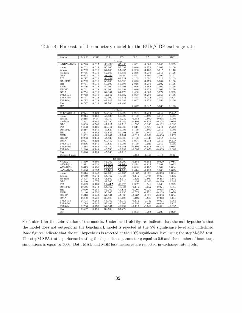
Table 4: Forecasts of the monetary model for the EUR/GBP exchange rate
Model MAE MSE DA DV RS RF SRS SRF
1-stepr-BDVAR(2) 0.743 0.017 56.250 65.490 4.831 4.602 0.248 0.235
mean 0.762 0.018 50.000 56.698 2.046 3.279 0.102 0.166tmean 0.762 0.018 52.083 57.435 2.286 3.488 0.115 0.176median 0.765 0.018 52.083 57.435 2.286 3.279 0.115 0.166OLS 0.923 0.037 58.333 56.26 1.897 3.300 0.095 0.167PC 0.717 0.017 56.250 63.221 4.163 2.057 0.212 0.103DMSFE 0.762 0.018 50.000 56.698 2.046 3.279 0.102 0.166HR 0.761 0.018 50.000 56.698 2.046 3.279 0.102 0.166EHR 0.756 0.018 50.000 56.698 2.046 3.488 0.102 0.176EEDF 0.761 0.018 50.000 56.698 2.046 3.279 0.102 0.166BMA 0.754 0.018 54.167 61.178 3.400 4.602 0.172 0.235FMA-aic 0.773 0.018 47.917 53.682 1.067 3.279 0.053 0.166FMA-bic 0.771 0.018 50.000 55.138 1.545 4.014 0.077 0.204FMA-hq 0.772 0.018 47.917 53.682 1.067 3.279 0.053 0.166RW 0.747 0.018 37.500 44.459CT 2.647 2.647 0.133 0.133
6-stepsrs-DVAR(1) 2.021 0.121 60.417 57.300 1.004 2.274 0.117 0.273
mean 2.214 0.139 45.833 50.908 0.130 -0.070 0.015 -0.008tmean 2.218 0.14 43.750 46.232 -0.558 -0.070 -0.065 -0.008median 2.257 0.146 43.750 43.745 -0.892 0.176 -0.104 0.020OLS 3.863 0.566 47.917 38.710 -1.550 -0.283 -0.182 -0.033PC 1.883 0.106 60.417 62.368 1.811 2.660 0.214 0.323
DMSFE 2.217 0.140 45.833 50.908 0.130 -0.070 0.015 -0.008HR 2.223 0.141 45.833 50.908 0.130 -0.070 0.015 -0.008EHR 2.532 0.184 41.667 47.781 -0.313 -1.528 -0.036 -0.179EEDF 2.236 0.142 45.833 50.908 0.130 -0.448 0.015 -0.052BMA 2.021 0.121 60.417 57.300 1.004 2.274 0.117 0.273
FMA-aic 2.266 0.146 45.833 50.908 0.130 -0.229 0.015 -0.027FMA-bic 2.218 0.141 43.750 43.751 -0.892 0.118 -0.104 0.014FMA-hq 2.246 0.144 43.750 46.232 -0.558 -0.070 -0.065 -0.008RW 2.046 0.124 45.833 42.113Forward rate -1.453 -1.453 -0.17 -0.17
12-stepsVAR(2) 3.340 0.399 54.167 48.290 -0.155 0.452 -0.029 0.084r-VAR(2) 2.881 0.334 62.500 54.921 0.474 0.123 0.088 0.023s-VAR(2) 3.419 0.430 56.250 49.965 0.008 0.452 0.002 0.084
rs-VAR(2) 2.896 0.337 62.500 54.921 0.474 0.123 0.088 0.023mean 2.614 0.242 52.083 46.165 -0.367 0.021 -0.068 0.004tmean 2.640 0.242 54.167 48.934 -0.112 -0.705 -0.021 -0.132median 2.808 0.258 41.667 38.170 -1.121 -0.967 -0.213 -0.182OLS 8.240 2.677 37.500 33.624 -1.453 -1.300 -0.280 -0.249PC 2.099 0.161 60.417 53.818 0.367 1.541 0.068 0.299DMSFE 2.646 0.244 54.167 48.934 -0.112 -0.352 -0.021 -0.065HR 2.640 0.250 54.167 47.833 -0.207 0.021 -0.038 0.004EHR 3.146 0.350 50.000 43.850 -0.579 0.271 -0.108 0.050EEDF 2.618 0.242 54.167 47.833 -0.207 0.021 -0.038 0.004BMA 2.838 0.230 39.583 38.106 -1.122 -0.817 -0.213 -0.153FMA-aic 2.703 0.254 54.167 48.934 -0.112 -0.352 -0.021 -0.065FMA-bic 2.715 0.246 52.083 46.362 -0.355 -0.933 -0.066 -0.176FMA-hq 2.706 0.250 54.167 48.934 -0.112 -0.512 -0.021 -0.095RW 2.597 0.193 39.583 37.279CT 1.203 1.203 0.229 0.229
See Table 1 for the abbreviation of the models. Underlined bold figures indicate that the null hypothesis that
the model does not outperform the benchmark model is rejected at the 5% significance level and underlined
italic figures indicate that the null hypothesis is rejected at the 10% significance level using the stepM-SPA test.
The stepM-SPA test is performed setting the dependence parameter q equal to 0.9 and the number of bootstrap
simulations is equal to 5000. Both MAE and MSE loss measures are reported in exchange rate levels.
32

Table 5: Forecasts of the capital flows model for the EUR/GBP exchange rate
Model MAE MSE DA DV RS RF SRS SRF
1-stepr-VEC(2,11) 0.771 0.020 58.333 63.603 4.169 3.293 0.212 0.166rs-DVAR(1) 0.767 0.019 56.250 61.328 3.447 5.577 0.174 0.289r-BDVAR(2) 0.755 0.018 56.250 61.328 3.447 4.842 0.174 0.249mean 0.769 0.018 52.083 54.182 1.219 2.792 0.061 0.140tmean 0.770 0.018 52.083 54.182 1.219 2.792 0.061 0.140median 0.765 0.018 50.000 58.395 2.535 4.223 0.127 0.215OLS 0.998 0.038 64.583 70.682 6.659 7.716 0.352 0.417
PC 0.731 0.017 62.500 65.624 4.914 4.261 0.252 0.217DMSFE 0.770 0.018 52.083 54.182 1.219 2.792 0.061 0.140HR 0.770 0.018 52.083 54.182 1.219 2.792 0.061 0.140EHR 0.771 0.018 52.083 57.783 2.301 4.734 0.115 0.243EEDF 0.770 0.018 52.083 54.182 1.219 2.792 0.061 0.140BMA 0.767 0.019 56.250 61.328 3.447 5.577 0.174 0.289FMA-aic 0.779 0.019 50.000 56.754 2.024 4.223 0.101 0.215FMA-bic 0.779 0.019 47.917 54.522 1.296 4.223 0.065 0.215FMA-hq 0.779 0.019 47.917 54.908 1.415 4.223 0.071 0.215RW 0.747 0.018 37.500 44.459CT 2.647 2.647 0.133 0.133
6-stepsDVAR(3) 2.161 0.132 52.083 57.764 1.056 2.355 0.123 0.283rsDVAR(1) 2.018 0.120 58.333 56.977 0.960 1.339 0.112 0.157mean 2.264 0.145 54.167 51.152 0.198 0.548 0.023 0.063tmean 2.230 0.141 50.000 46.073 -0.541 0.979 -0.063 0.114median 2.149 0.133 54.167 50.139 0.060 1.439 0.007 0.169OLS 3.659 0.455 54.167 44.362 -0.849 -1.066 -0.098 -0.124PC 1.964 0.108 56.250 58.709 1.283 1.787 0.150 0.211DMSFE 2.264 0.144 52.083 48.499 -0.171 0.646 -0.020 0.075HR 2.285 0.147 47.917 45.034 -0.678 0.548 -0.079 0.063NESHR 2.441 0.172 47.917 43.351 -0.919 -0.115 -0.107 -0.013EEFF 2.298 0.149 47.917 44.945 -0.698 0.548 -0.081 0.063BMA 2.018 0.120 58.333 56.977 0.960 1.339 0.112 0.157FMA-aic 2.280 0.145 52.083 50.738 0.124 0.700 0.014 0.081FMA-bic 2.289 0.147 45.833 46.794 -0.449 0.849 -0.052 0.099FMA-hq 2.284 0.146 50.000 48.141 -0.261 0.849 -0.030 0.099RW 2.046 0.124 45.833 42.113Forward rate -1.453 -1.453 -0.17 -0.17
12-stepsrs-VAR(2) 2.629 0.229 58.333 52.261 0.213 -0.310 0.040 -0.058r-BDVAR(2) 2.756 0.219 39.583 37.629 -1.177 -0.415 -0.224 -0.077mean 2.871 0.273 45.833 38.509 -1.015 -1.701 -0.192 -0.333tmean 2.846 0.264 47.917 40.059 -0.875 -1.171 -0.164 -0.223median 2.835 0.253 37.500 31.666 -1.668 -0.762 -0.325 -0.143OLS 12.622 38.375 20.833 15.648 -3.136 -3.136 -0.718 -0.718PC 2.068 0.155 64.583 59.773 0.919 1.297 0.173 0.248DMSFE 2.815 0.271 45.833 38.509 -1.015 -1.246 -0.192 -0.238HR 2.883 0.282 41.667 31.993 -1.597 -1.451 -0.310 -0.280EHR 2.979 0.322 52.083 41.418 -0.751 -1.080 -0.141 -0.204EEDF 2.874 0.280 41.667 31.993 -1.597 -1.451 -0.310 -0.280BMA 2.792 0.223 35.417 35.457 -1.366 -0.756 -0.262 -0.142FMA-aic 2.785 0.265 60.417 51.790 0.176 -0.787 0.033 -0.147FMA-bic 2.804 0.269 58.333 50.445 0.055 -0.950 0.010 -0.179FMA-hq 2.792 0.267 60.417 51.790 0.176 -0.787 0.033 -0.147RW 2.597 0.193 39.583 37.279CT 1.203 1.203 0.229 0.229
See Table 1 for the abbreviation of the models. Underlined bold figures indicate that the null hypothesis that
the model does not outperform the benchmark model is rejected at the 5% significance level and underlined
italic figures indicate that the null hypothesis is rejected at the 10% significance level using the stepM-SPA test.
The stepM-SPA test is performed setting the dependence parameter q equal to 0.9 and the number of bootstrap
simulations is equal to 5000. Both MAE and MSE loss measures are reported in exchange rate levels.
33

Table 6: Forecasts of the monetary model for the EUR/CHF exchange rate
Model MAE MSE DA DV RS RF SRS SRF
1-stepDVAR(2) 0.460 0.013 68.750 64.870 4.641 6.311 0.202 0.279BDVAR(2) 0.450 0.012 64.583 62.389 3.898 6.261 0.168 0.277r-BDVAR(2) 0.455 0.012 62.500 63.501 4.257 9.435 0.184 0.440mean 0.458 0.013 62.500 62.971 4.105 6.006 0.178 0.265tmean 0.458 0.013 64.583 63.520 4.262 6.006 0.185 0.265median 0.458 0.013 64.583 63.520 4.262 5.930 0.185 0.261OLS 0.596 0.019 52.083 50.615 0.444 3.450 0.019 0.149PC 0.532 0.014 35.417 35.873 -4.479 10.100 -0.194 0.478DMSFE 0.458 0.013 62.500 62.971 4.105 6.006 0.178 0.265HR 0.458 0.013 62.500 62.971 4.105 6.006 0.178 0.265EHR 0.464 0.013 62.500 64.235 4.486 6.367 0.195 0.282EEDF 0.458 0.013 62.500 62.971 4.105 6.007 0.178 0.265BMA 0.453 0.012 62.500 61.310 3.596 5.975 0.155 0.263FMA-aic 0.462 0.013 66.667 64.795 4.620 6.338 0.201 0.281FMA-bic 0.459 0.013 66.667 64.795 4.620 6.338 0.201 0.281FMA-hq 0.461 0.013 66.667 64.795 4.620 6.338 0.201 0.281RW 0.466 0.012 66.667 66.147CT 5.092 5.092 0.222 0.222
6-stepsDVAR(2) 1.294 0.064 68.750 83.363 5.204 3.464 0.604 0.366
mean 1.458 0.075 47.917 67.096 2.656 -0.505 0.273 -0.050tmean 1.443 0.074 52.083 71.446 3.282 -0.505 0.344 -0.050median 1.407 0.071 54.167 72.901 3.486 0.905 0.369 0.090OLS 2.466 0.212 43.750 52.811 0.192 0.505 0.019 0.050PC 1.681 0.100 31.250 9.990 -6.127 -3.588 -0.769 -0.381DMSFE 1.446 0.074 52.083 71.446 3.282 -0.505 0.344 -0.050HR 1.436 0.073 54.167 72.901 3.486 0.725 0.369 0.072EHR 1.388 0.067 54.167 72.901 3.486 1.021 0.369 0.102EEDF 1.428 0.072 58.333 76.551 4.111 0.841 0.447 0.084BMA 1.354 0.066 62.500 81.122 4.891 1.722 0.556 0.173FMA-aic 1.453 0.074 50.000 67.479 2.710 -0.267 0.279 -0.026FMA-bic 1.429 0.072 47.917 67.096 2.656 -0.267 0.273 -0.026FMA-hq 1.443 0.073 50.000 67.479 2.710 -0.267 0.279 -0.026RW 1.382 0.070 62.500 82.865CT 5.160 5.160 0.597 0.597
12-stepsDVAR(2) 2.233 0.155 70.833 88.077 5.143 3.643 0.795 0.490s-DVAR(1) 2.191 0.147 68.750 87.814 5.111 3.638 0.787 0.489mean 2.561 0.193 54.167 66.945 2.163 -1.722 0.270 -0.212tmean 2.531 0.189 54.167 66.945 2.163 -1.403 0.270 -0.172median 2.406 0.174 66.667 84.990 4.707 1.281 0.692 0.156OLS 6.001 1.110 18.750 11.034 -5.187 -5.156 -0.806 -0.798PC 2.881 0.255 25.000 7.969 -5.605 -5.035 -0.924 -0.768DMSFE 2.513 0.187 56.250 70.478 2.665 -1.913 0.339 -0.237HR 2.462 0.181 64.583 83.261 4.500 -0.608 0.648 -0.073EHR 2.370 0.167 68.750 87.814 5.111 -0.306 0.787 -0.037
EEDF 2.446 0.179 66.667 84.856 4.733 -0.106 0.698 -0.013BMA 2.292 0.157 68.750 87.814 5.111 3.638 0.787 0.489FMA-aic 2.557 0.189 52.083 69.145 2.501 -1.328 0.316 -0.162FMA-bic 2.496 0.182 54.167 72.677 3.003 -0.455 0.389 -0.055FMA-hq 2.532 0.186 52.083 69.145 2.501 -1.011 0.316 -0.123RW 2.384 0.182 68.750 87.814CT 5.751 5.751 0.971 0.971
See Table 1 for the abbreviation of the models. Underlined bold figures indicate that the null hypothesis that
the model does not outperform the benchmark model is rejected at the 5% significance level and underlined
italic figures indicate that the null hypothesis is rejected at the 10% significance level using the stepM-SPA test.
The stepM-SPA test is performed setting the dependence parameter q equal to 0.9 and the number of bootstrap
simulations is equal to 5000. Both MAE and MSE loss measures are reported in exchange rate levels.
34
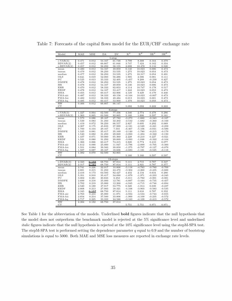
Table 7: Forecasts of the capital flows model for the EUR/CHF exchange rate
Model MAE MSE DA DV RS RF SRS SRF
1-stepr-VAR(3) 0.471 0.012 54.167 61.748 3.799 8.308 0.164 0.379BDVAR(2) 0.457 0.012 66.667 61.846 3.747 7.424 0.162 0.334r-BDVAR(2) 0.457 0.012 56.250 58.155 2.698 10.476 0.116 0.500mean 0.480 0.012 54.167 49.859 0.140 10.023 0.006 0.473tmean 0.479 0.012 56.250 53.535 1.275 10.023 0.054 0.473median 0.477 0.012 56.250 53.535 1.275 10.317 0.054 0.491OLS 0.641 0.019 52.083 56.286 1.905 2.586 0.081 0.111PC 0.525 0.013 33.333 32.405 -5.457 9.209 -0.239 0.427DMSFE 0.478 0.012 56.250 53.535 1.275 10.023 0.054 0.473HR 0.478 0.012 54.167 49.859 0.140 10.023 0.006 0.473EHR 0.470 0.012 58.333 62.853 4.114 10.747 0.178 0.517EEDF 0.478 0.012 54.167 53.417 1.242 10.023 0.053 0.473BMA 0.455 0.012 60.417 62.906 4.129 9.429 0.179 0.440FMA-aic 0.487 0.012 58.333 49.158 -0.164 10.023 -0.007 0.473FMA-bic 0.482 0.012 58.333 49.484 0.013 10.023 0.001 0.473FMA-hq 0.485 0.012 60.417 53.900 1.379 10.023 0.059 0.473RW 0.466 0.012 66.667 66.147CT 5.092 5.092 0.222 0.222
6-stepsr-VAR(3) 1.327 0.064 62.500 77.336 4.346 2.774 0.478 0.286r-BDVAR(2) 1.363 0.065 62.500 82.865 5.160 1.606 0.597 0.161mean 1.573 0.086 29.167 27.782 -3.273 -1.660 -0.343 -0.167tmean 1.539 0.083 31.250 32.202 -2.542 -1.682 -0.260 -0.169median 1.419 0.072 56.250 66.557 2.827 0.695 0.292 0.069OLS 2.307 0.175 45.833 37.999 -2.181 -2.529 -0.221 -0.259PC 1.700 0.104 29.167 7.555 -6.467 -5.106 -0.841 -0.589DMSFE 1.525 0.081 35.417 35.169 -2.120 -1.780 -0.215 -0.179HR 1.540 0.082 31.250 29.069 -3.093 -1.494 -0.322 -0.150EHR 1.437 0.071 50.000 65.360 2.228 -0.210 0.227 -0.021EEDF 1.521 0.080 31.250 29.069 -3.093 -1.048 -0.322 -0.104BMA 1.366 0.066 60.417 74.215 3.820 0.774 0.410 0.077FMA-aic 1.612 0.090 25.000 11.947 -5.796 -2.899 -0.705 -0.300FMA-bic 1.551 0.084 39.583 39.859 -1.275 -0.797 -0.127 -0.079FMA-hq 1.587 0.087 29.167 18.606 -4.683 -1.181 -0.525 -0.118RW 1.382 0.070 62.500 82.865CT 5.160 5.160 0.597 0.597
12-stepsr-DVAR(3) 2.323 0.155 68.750 87.814 5.111 2.715 0.787 0.347BDVAR(2) 2.317 0.161 68.750 87.814 5.111 2.921 0.787 0.377mean 2.741 0.226 22.917 10.808 -5.118 -4.783 -0.789 -0.709tmean 2.681 0.215 31.250 24.470 -3.304 -4.260 -0.435 -0.600median 2.416 0.173 64.583 82.427 4.432 2.134 0.634 0.266OLS 5.351 0.910 35.417 34.090 -1.879 -1.971 -0.233 -0.245PC 3.002 0.281 20.833 6.252 -5.811 -5.782 -0.991 -0.981DMSFE 2.699 0.218 25.000 12.781 -4.897 -3.444 -0.735 -0.457HR 2.702 0.219 25.000 12.200 -4.945 -4.715 -0.746 -0.694EHR 2.520 0.189 47.917 53.775 0.320 -1.914 0.039 -0.237EEDF 2.668 0.213 27.083 18.321 -4.168 -3.903 -0.583 -0.535BMA 2.345 0.157 68.750 87.814 5.111 2.616 0.787 0.332FMA-aic 2.763 0.233 25.000 11.871 -4.934 -4.534 -0.744 -0.655FMA-bic 2.654 0.214 37.500 33.806 -1.900 -4.109 -0.235 -0.572FMA-hq 2.717 0.225 33.333 24.588 -3.163 -4.109 -0.413 -0.572RW 2.384 0.182 68.750 87.814CT 5.751 5.751 0.971 0.971
See Table 1 for the abbreviation of the models. Underlined bold figures indicate that the null hypothesis that
the model does not outperform the benchmark model is rejected at the 5% significance level and underlined
italic figures indicate that the null hypothesis is rejected at the 10% significance level using the stepM-SPA test.
The stepM-SPA test is performed setting the dependence parameter q equal to 0.9 and the number of bootstrap
simulations is equal to 5000. Both MAE and MSE loss measures are reported in exchange rate levels.
35
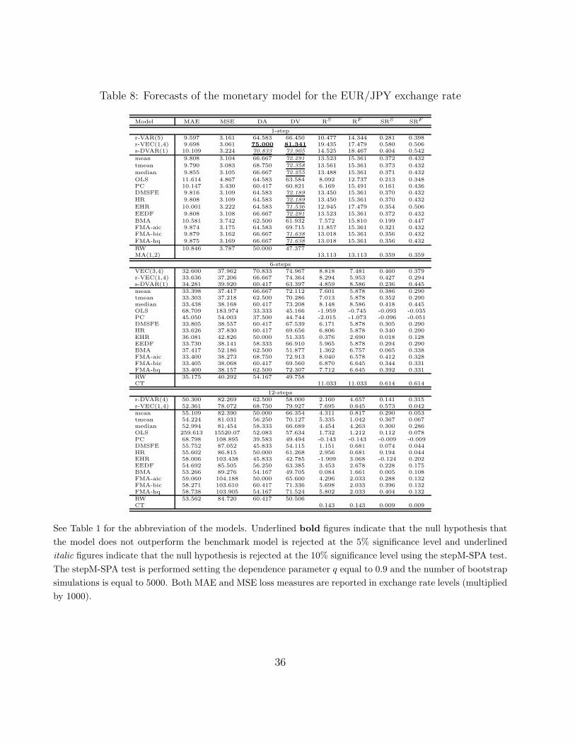
Table 8: Forecasts of the monetary model for the EUR/JPY exchange rate
Model MAE MSE DA DV RS RF SRS SRF
1-stepr-VAR(5) 9.597 3.161 64.583 66.450 10.477 14.344 0.281 0.398r-VEC(1,4) 9.698 3.061 75.000 81.341 19.435 17.479 0.580 0.506s-DVAR(1) 10.109 3.224 70.833 73.905 14.525 18.467 0.404 0.542
mean 9.808 3.104 66.667 72.291 13.523 15.361 0.372 0.432
tmean 9.790 3.083 68.750 72.358 13.561 15.361 0.373 0.432median 9.855 3.105 66.667 72.255 13.488 15.361 0.371 0.432
OLS 11.614 4.867 64.583 63.584 8.092 12.737 0.213 0.348PC 10.147 3.430 60.417 60.821 6.169 15.491 0.161 0.436DMSFE 9.816 3.109 64.583 72.189 13.450 15.361 0.370 0.432HR 9.808 3.109 64.583 72.189 13.450 15.361 0.370 0.432
EHR 10.001 3.222 64.583 71.536 12.945 17.479 0.354 0.506EEDF 9.808 3.108 66.667 72.291 13.523 15.361 0.372 0.432
BMA 10.581 3.742 62.500 61.932 7.572 15.810 0.199 0.447FMA-aic 9.874 3.175 64.583 69.715 11.857 15.361 0.321 0.432FMA-bic 9.879 3.162 66.667 71.638 13.018 15.361 0.356 0.432FMA-hq 9.875 3.169 66.667 71.638 13.018 15.361 0.356 0.432
RW 10.846 3.787 50.000 47.377MA(1,2) 13.113 13.113 0.359 0.359
6-stepsVEC(3,4) 32.600 37.962 70.833 74.967 8.818 7.481 0.460 0.379r-VEC(1,4) 33.636 37.206 66.667 74.364 8.294 5.953 0.427 0.294s-DVAR(1) 34.281 39.920 60.417 63.397 4.859 8.586 0.236 0.445mean 33.398 37.417 66.667 72.112 7.601 5.878 0.386 0.290tmean 33.303 37.218 62.500 70.286 7.013 5.878 0.352 0.290median 33.438 38.168 60.417 73.208 8.148 8.586 0.418 0.445OLS 68.709 183.974 33.333 45.166 -1.959 -0.745 -0.093 -0.035PC 45.050 54.003 37.500 44.744 -2.015 -1.073 -0.096 -0.051DMSFE 33.805 38.557 60.417 67.539 6.171 5.878 0.305 0.290HR 33.626 37.830 60.417 69.656 6.806 5.878 0.340 0.290EHR 36.081 42.826 50.000 51.335 0.376 2.690 0.018 0.128EEDF 33.730 38.141 58.333 66.910 5.965 5.878 0.294 0.290BMA 37.417 52.186 62.500 51.877 1.362 6.757 0.065 0.338FMA-aic 33.400 38.273 68.750 72.913 8.040 6.578 0.412 0.328FMA-bic 33.405 38.068 60.417 69.560 6.870 6.645 0.344 0.331FMA-hq 33.400 38.157 62.500 72.307 7.712 6.645 0.392 0.331RW 35.175 40.292 54.167 49.758CT 11.033 11.033 0.614 0.614
12-stepsr-DVAR(4) 50.300 82.269 62.500 58.000 2.160 4.657 0.141 0.315r-VEC(1,4) 52.361 78.072 68.750 79.927 7.695 0.645 0.573 0.042mean 55.109 82.390 50.000 66.354 4.311 0.817 0.290 0.053tmean 54.224 81.031 56.250 70.127 5.335 1.042 0.367 0.067median 52.994 81.454 58.333 66.689 4.454 4.263 0.300 0.286OLS 259.613 15520.07 52.083 57.634 1.732 1.212 0.112 0.078PC 68.798 108.895 39.583 49.494 -0.143 -0.143 -0.009 -0.009DMSFE 55.752 87.052 45.833 54.115 1.151 0.681 0.074 0.044HR 55.602 86.815 50.000 61.268 2.956 0.681 0.194 0.044EHR 58.006 103.438 45.833 42.785 -1.909 3.068 -0.124 0.202EEDF 54.692 85.505 56.250 63.385 3.453 2.678 0.228 0.175BMA 53.266 89.276 54.167 49.705 0.084 1.661 0.005 0.108FMA-aic 59.060 104.188 50.000 65.600 4.296 2.033 0.288 0.132FMA-bic 58.271 103.610 60.417 71.336 5.698 2.033 0.396 0.132FMA-hq 58.738 103.905 54.167 71.524 5.802 2.033 0.404 0.132RW 53.562 84.720 60.417 50.506CT 0.143 0.143 0.009 0.009
See Table 1 for the abbreviation of the models. Underlined bold figures indicate that the null hypothesis that
the model does not outperform the benchmark model is rejected at the 5% significance level and underlined
italic figures indicate that the null hypothesis is rejected at the 10% significance level using the stepM-SPA test.
The stepM-SPA test is performed setting the dependence parameter q equal to 0.9 and the number of bootstrap
simulations is equal to 5000. Both MAE and MSE loss measures are reported in exchange rate levels (multiplied
by 1000).
36
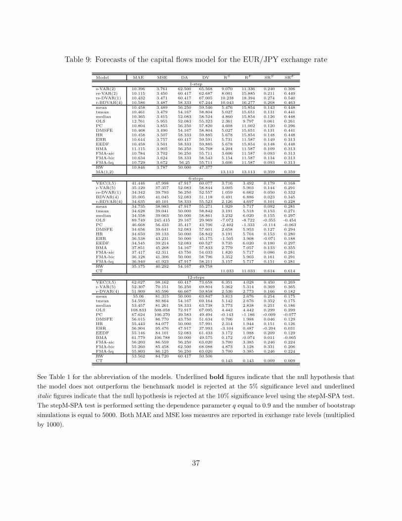
Table 9: Forecasts of the capital flows model for the EUR/JPY exchange rate
Model MAE MSE DA DV RS RF SRS SRF
1-steps-VAR(2) 10.396 3.761 62.500 65.568 9.070 11.336 0.240 0.306rs-VAR(2) 10.115 3.450 60.417 62.687 8.001 15.885 0.211 0.449rs-DVAR(1) 10.432 3.471 60.417 67.005 10.238 18.394 0.274 0.540r-BDVAR(4) 10.586 3.487 58.333 67.244 10.043 16.277 0.268 0.463mean 10.458 3.489 56.250 59.546 5.476 15.854 0.143 0.448tmean 10.461 3.479 54.167 58.804 5.027 15.651 0.131 0.441median 10.365 3.415 52.083 58.524 4.860 15.854 0.126 0.448OLS 12.761 5.955 52.083 55.323 2.361 9.797 0.061 0.261PC 10.804 3.855 56.250 57.820 4.608 11.002 0.120 0.296DMSFE 10.468 3.490 54.167 58.804 5.027 15.651 0.131 0.441HR 10.458 3.507 58.333 59.885 5.678 15.854 0.148 0.448EHR 10.644 3.757 60.417 59.591 5.731 11.587 0.149 0.313EEDF 10.458 3.501 58.333 59.885 5.678 15.854 0.148 0.448BMA 11.115 3.905 56.250 56.768 4.204 11.587 0.109 0.313FMA-aic 10.784 3.702 56.250 55.711 3.606 11.587 0.093 0.313FMA-bic 10.634 3.624 58.333 58.543 5.154 11.587 0.134 0.313FMA-hq 10.729 3.672 56.25 55.711 3.606 11.587 0.093 0.313RW 10.846 3.787 50.000 47.377MA(1,2) 13.113 13.113 0.359 0.359
6-stepsVEC(3,5) 41.446 47.998 47.917 60.077 3.716 3.492 0.179 0.168r-VAR(5) 35.120 37.357 52.083 58.844 3.005 5.903 0.144 0.291rs-DVAR(1) 34.342 39.793 56.250 52.557 1.059 6.662 0.050 0.332BDVAR(4) 35.005 41.045 52.083 51.118 0.491 6.886 0.023 0.345r-BDVAR(4) 34.635 40.101 58.333 55.523 2.126 4.697 0.101 0.228mean 34.735 38.983 47.917 55.271 1.929 5.717 0.092 0.281tmean 34.628 39.041 50.000 58.842 3.191 5.518 0.153 0.271median 34.558 39.063 50.000 58.861 3.232 6.020 0.155 0.297OLS 89.749 245.415 29.167 29.969 -7.072 -8.722 -0.355 -0.454PC 46.668 56.433 35.417 43.706 -2.402 -1.333 -0.114 -0.063DMSFE 34.656 39.641 52.083 57.601 2.658 5.953 0.127 0.294HR 34.650 39.133 50.000 58.842 3.191 5.704 0.153 0.280EHR 36.538 43.231 50.000 45.175 -1.505 3.908 -0.071 0.188EEDF 34.545 39.214 52.083 60.527 3.735 6.020 0.180 0.297BMA 37.851 45.268 54.167 57.833 2.779 7.057 0.133 0.355FMA-aic 37.417 42.311 43.750 54.033 1.820 5.717 0.086 0.281FMA-bic 36.128 41.306 50.000 58.796 3.352 5.903 0.161 0.291FMA-hq 36.940 41.923 47.917 58.211 3.157 5.717 0.151 0.281RW 35.175 40.292 54.167 49.758CT 11.033 11.033 0.614 0.614
12-stepsVEC(3,5) 62.027 98.162 60.417 73.658 6.351 4.028 0.450 0.269r-VAR(5) 52.307 70.151 56.250 69.804 5.362 5.314 0.369 0.365r-DVAR(4) 51.909 85.596 66.667 59.858 2.536 2.773 0.166 0.182mean 55.06 81.315 50.000 63.847 3.813 2.676 0.254 0.175tmean 54.593 80.864 54.167 69.164 5.142 2.676 0.352 0.175median 53.457 81.261 58.333 63.738 3.773 2.838 0.251 0.186OLS 108.833 508.058 72.917 67.095 4.442 4.442 0.299 0.299PC 67.624 106.270 39.583 49.494 -0.143 -1.186 -0.009 -0.077DMSFE 56.015 86.770 43.750 51.634 0.706 1.988 0.046 0.129HR 55.443 84.077 50.000 57.991 2.314 1.944 0.151 0.126EHR 56.904 95.476 47.917 37.993 -3.104 0.487 -0.204 0.031EEDF 55.146 84.101 52.083 61.433 3.172 1.988 0.209 0.129BMA 61.779 106.788 50.000 49.575 0.172 -0.074 0.011 -0.005FMA-aic 56.203 86.559 56.250 63.020 3.700 3.385 0.246 0.224FMA-bic 55.260 85.458 62.500 68.088 4.873 3.128 0.331 0.206FMA-hq 55.803 86.125 56.250 63.020 3.700 3.385 0.246 0.224RW 53.562 84.720 60.417 50.506CT 0.143 0.143 0.009 0.009
See Table 1 for the abbreviation of the models. Underlined bold figures indicate that the null hypothesis that
the model does not outperform the benchmark model is rejected at the 5% significance level and underlined
italic figures indicate that the null hypothesis is rejected at the 10% significance level using the stepM-SPA test.
The stepM-SPA test is performed setting the dependence parameter q equal to 0.9 and the number of bootstrap
simulations is equal to 5000. Both MAE and MSE loss measures are reported in exchange rate levels (multiplied
by 1000).
37


![OUTPERFORM [V] INITIATION](https://img.pdfslide.net/doc/110x75/6189e5c61eda5f71d25deb98/outperform-v-initiation.jpg)