Can Risk Management Help Prevent Bankruptcy?

Monica Marin∗

July, 2007

Abstract

Whether companies engage in risk management activities for risk reduction or speculation purposeshas been subject to continuous debate. This paper compares the use of risk management instrumentsby firms that eventually file for bankruptcy to matched firms that do not file for bankruptcy duringthe sample period. Results indicate that the odds of filing for bankruptcy are approximately 96% lowerfor firms that manage risk. The paper also takes an alternative approach in predicting the probabilityof default by deriving the distance to default from equity prices with the Black-Scholes-Merton optionpricing model. The distance to default compares the market value of assets to the size of a one standarddeviation move in the asset value. Results show that the number of standard deviations by which firmsin the sample are away from the default point increases by 3.2 units when they engage in risk manage-ment activities. The main findings are reinforced when examining the equity-implied asset volatilityas a separate measure of firm risk and its relationship with risk management. More specifically, assetvolatility decreases by 64% when firms manage risk.

∗Moore School of Business, University of South Carolina, Columbia, SC 29208. E-mail:monica marin@moore.sc.edu

1 Introduction

In the 2002 Berkshire Hathaway annual report, Warren Buffet warned against the use of

derivatives, referring to them as ”financial weapons of mass destruction, carrying dangers

that, while now latent, are potentially lethal.” His view on derivatives opposes the classical

belief that they are used to reduce risk (Smith and Stulz (1985)), being known primarily as

hedging instruments. While most of the concern over the use of derivatives has been expressed

by practitioners, a recent academic study (Faulkender (2005)) shows that firms often use in-

terest rate risk management instruments to time the market.

I provide evidence on whether risk management instruments are used for risk reduction

purposes by examining whether the use of risk management instruments reduces the probabil-

ity of financial distress. This question has been investigated by several academic studies, but

the evidence is limited. Nance, Smith, and Smithson (1993), and Mian (1996)) do not find any

relation between the use of derivatives and the probability of bankruptcy, while Fok, Carroll,

and Chiou (1997) find a weak negative relation. More recently, Judge (2003) shows a strong

negative relation in a study examining the risk management activity of U.K. firms. He also

finds a stronger relation for the U.K. firms than for the U.S. firms, and attributes this result to

differences in the bankruptcy codes. Unlike the previous studies that analyze solely the use of

derivatives, Judge (2003) uses a broader definition of risk management activity, that includes

both financial derivatives and hedging methods other than financial derivatives.

I use a pair-matched sample of U.S. bankrupt and non-bankrupt companies between 1998

and 2005, and estimate a duration analysis model for the likelihood of bankruptcy as a function

of their risk management activity. Second, I estimate the distance to default with a structural

model and then evaluate whether risk management helps to explain the distance to default.

Last, I investigate the relationship between risk management and the equity-implied asset

volatility as an alternative measure of firm risk.

A word of caution is necessary given that the sample of bankrupt and non-bankrupt firms

1

is a non-random sub-sample of public companies. If risk management is driven by reasons of

financial distress and bankruptcy costs, then this sample is biased towards firms where risk

management is most desirable. Therefore, inferences about the impact of risk management

on firms’ riskiness should not be made beyond this sample. However, if financial distress is

one of the primary determinants of risk management, then the analysis of bankrupt and non-

bankrupt firms would probably provide the most interesting insights.

The sample of 344 bankrupt and non-bankrupt firms is restricted to those non-financial

and non-utility firms that have available accounting data (from Compustat), as well as risk

management information disclosed in their annual reports for at least one year prior to filing

for bankruptcy. I define a firm as engaging in risk management in a particular year if the firm

uses any risk management instruments, including both financial derivative instruments and

methods other than financial derivatives. For example, I classify a firm as engaging in risk

management if the firm reports a fixed rate debt issue as a hedging activity under SFAS 133

(Accounting for Derivative Instruments and for Hedging Activities). As Faulkender (2005),

Kedia and Mozumdar (2003), and Judge (2003) argue, this approach provides a more accurate

picture of a firm’s risk management strategy than simply using derivative use to classify firms

as engaging in risk management. In addition, to identify whether a company engages in any

type of risk management, I also identify whether a firm engages in interest rate risk manage-

ment, foreign currency risk management, or commodity price risk management. I follow each

firm in time, starting with the first year when it discloses its position on risk management (can

be as early as 1994) and ending with the fiscal year before bankruptcy filing (can be as late as

2004).

I first estimate a discrete time complementary loglog hazard model for firms’ probability

to file for bankruptcy within one year. The duration analysis approach is more appropriate for

my sample and, according to Shumway (2001), it performs better than the conditional binary

models that are widely used. Since the likelihood of financial distress could influence the use

2

of risk management instruments, I use GMM (Generalized Method of Moments) models to

control for the endogeneity between the probability of bankruptcy and the risk management

decision.

I find that, all else equal, the odds of filing for bankruptcy are 96% lower for the firms

that manage risk as opposed to the ones that do not. This result suggests that the use of risk

management instruments helps reduce risk and extend a firm’s life.

Second, I estimate the distance to default from equity prices in a Black-Scholes-Merton

option pricing framework. The distance to default measures how far (in terms of the number

of standard deviations) the firm’s asset value is from the default point. Next, I estimate a

GMM model to study the relationship between risk management and the distance to default.

The results obtained with this approach are consistent with those from the duration analy-

sis approach. All else equal, any risk management activity is associated with a higher distance

to default. On average, the number of standard deviations by which firms are away from the

default point increases by 3.2 units when they manage risk. This evidence confirms the finding

from the cloglog model, namely that engaging in risk management activities tends to reduce

the probability of default.

Third, I investigate the relationship between risk management and the equity-implied asset

volatility1 as a distinct measure of firm risk, and estimate a GMM model that accounts for

the endogenous regressors.

The results confirm the previous findings in the paper and show that, all else equal, firms

that use risk management instruments have a significantly lower asset volatility. More specifi-

cally, on average firms’ asset volatility is reduced by 64% when they manage risk. Furthermore,

separate analysis of interest rate risk management and foreign currency risk management in-

dicate that these are also associated with lower asset volatility.

As a first robustness check, I investigate the relationship between the changes in the dis-

1Asset volatility is also used in the distance to default calculation, as shown in Section 3.2.

3

tance to default or asset volatility and the changes in the firms’ risk management activity.

I find that changes in the risk management activity in general are positively related to the

changes in the distance to default and negatively related to the changes in asset volatility,

results which are consistent with the main findings. In addition, a positive and significant

relationship is found between the changes in the distance to default and the changes in inter-

est rate risk management, as well as between the changes in the distance to default and the

changes in foreign currency risk management. On the other hand, the changes in commodity

price risk management are negatively associated with the changes in the distance to default,

which constitutes, counter-evidence to the risk-reduction hypothesis.

Next, I use sub-sample analysis to examine the relationship between risk management and

the distance to default or the asset volatility. I calculate the mean risk exposure (i.e. interest

rate risk exposure, foreign currency risk exposure, and commodity price risk exposure respec-

tively), and divide the sample into two sub-samples for high and low exposure in each of the

three categories. Most of the results support the main findings and suggest that, for firms

with high interest rate exposure or high foreign currency exposure, the distance to default is

augmented and asset volatility is reduced when they manage any type of risk or particular

risks (i.e. interest rate, foreign currency, commodity price risks). However, for firms with low

interest rate exposure and foreign currency exposure, the use of commodity price risk man-

agement instruments reduces the distance to default. Consequently, not only that the use of

commodity price risk management instruments does not benefit the firms with low interest

rate and foreign currency hedging needs, but also it may have a harmful effect. In terms of

the relationship between risk management and asset volatility for these firms, the negative

coefficient is consistent with the hypothesis of risk reduction. For firms with low commodity

price exposure, the use of risk management instruments increases the distance to default, while

decreasing asset volatility. At the same time, for firms with high commodity price exposure,

evidence shows only a negative relationship between interest rate risk management and asset

4

volatility.

Lastly, I examine the bankrupt and non-bankrupt firms separately, and find that, for each

category, firms that undertake risk management activities tend to have a lower asset volatility.

One contrasting result shows that for non-bankrupt firms, firms that manage interest rate risk

have a lower distance to default. Although this result may provide counter-evidence on the

risk-reduction purpose of interest rate risk management as shown by Faulkender (2005), it is

not confirmed in any other test.

Additional results which are consistent throughout this paper suggest that firm size is neg-

atively related to the odds of filing for bankruptcy and to asset volatility, and positively related

to the distance to default. Furthermore, leverage is associated with higher odds of filing for

bankruptcy, higher asset volatility, and lower distance to default.

As already mentioned, I obtain all empirical results reported in this paper using GMM

(Generalized Method of Moments). GMM estimates the model parameters without making

strong assumptions regarding the distributional properties of the variables observed. Thus, it

provides a solution to the case where the orthogonality assumption between the error term and

regressors is not satisfied. At the same time, it can be readily applied to nonlinear equations,

while providing a consistent estimate of the parameter.

In previous tests I also use a two-step procedure, where I first estimate a conditional binary

model (logit) to regress the risk management variable on appropriate explanatory variables.

Second, I include the predicted value in the cloglog and the linear regression models respec-

tively, along with other accounting-based determinants of the default probability, distance to

default, or asset volatility, while using the jackknife method to reduce the bias of the estimator

and to produce conservative standard errors. The final results obtained with this approach

are very similar, and thus not reported in the paper, but available upon request.

The paper is organized as follows: Section 2 presents a survey of the Related Literature,

Section 3 details the Empirical Estimation, Section 4 shows the Results, Section 5 presents

5

the robustness checks and their results, and Section 6 summarizes the Conclusions.

2 Related Literature

2.1 Why firms use risk management instruments

Smith and Stulz (1985) were among the first to recognize that transaction costs of bankruptcy

can induce public corporations to make use of risk management instruments.2 More specifi-

cally, they show that the use of risk management instruments can moderate the volatility of

cash flows, which reduces the probability of incurring direct and indirect bankruptcy costs.

As far as the empirical evidence is concerned, Nance, Smith, and Smithson (1993), and

Mian (1996)) do not find any relation between the use of derivatives and the probability of

bankruptcy. Later, Fok, Carroll, and Chiou (1997) find a weak negative relation between the

two. Only recently, Judge (2003) shows a strong negative relation for a sample of U.K. firms.

He attributes this difference relative to U.S. firms to dissimilarities in the bankruptcy codes.

Judge (2003) uses a broader definition of risk management activity, including both deriva-

tives and traditional hedging methods. On the other hand, another recent paper (Faulkender

(2005)) shows that interest rate risk management is driven by speculation or market timing.

However, instead of examining the use of derivatives, Faulkender (2005) investigates the de-

terminants of firms’ choices of interest rate exposure when issuing new debt, and finds that

these are related to the shape of the yield curve rather than to the hedging needs.

The existing literature has identified a multitude of factors contributing to a company’s

decision to manage risk. Smith and Stulz (1985) argue that the more wealth managers have

invested in the company (higher managerial ownership) the more they will tend to manage

risk. Tufano (1996) shows that a compensation contract that is linear or concave in firm value

provides incentives for the manager to reduce risk, while a convex contract has the opposite

2The costs of using risk management instruments are ignored throughout this paper.

6

effect. Consistent with this argument, he argues that managers of gold mining firms make

use of risk management instruments less if their compensation is based on stock options as

opposed to bonuses. Similarly, Rogers (2002) shows that derivative use is negatively related

to option holding and positively related to stock ownership.

Froot, Scharfstein, and Stein (1993) discuss other rationales for risk management in addi-

tion to the costs of financial distress and managerial incentives: taxes, debt capacity, capital

markets imperfections, and inefficient investment. Adam (2002) shows empirically that risk

management can reduce a firm’s dependence on external capital markets.

Empirical evidence by Mian (1996) shows that larger firms are more likely to manage risk,

companies that manage risk do not have higher market-to-book ratios, and risk management

is uncorrelated with leverage, positively correlated with dividend yield and dividend payout,

and negatively correlated with liquidity. Graham and Smith (1999) find that tax convexity

increases firms’ incentives to hedge.

Nevertheless, the relationship between firms’ use of risk management instruments and any

measure of firm riskiness or financial distress is most likely subject to an endogeneity problem.

For example, firms with a higher probability of financial distress may not be able to access cer-

tain risk management instruments that are available based on credit rating (i.e. interest rate

swaps). In their paper on dynamic risk management, Fehle and Tsyplakov (2005) demonstrate

that firms that are either far from financial distress or deep in financial distress do not initiate

or adjust their risk management instruments. On the other hand, they show that the rest of

the firms do initiate and actively adjust their use of risk management instruments. Similarly,

Purnanandam (2007) shows that financially distressed firms (that have high leverage) have

higher incentive to engage in hedging activities, but that these incentives disappear when their

financial distress becomes severe.

7

2.2 Factors Affecting the Probability of Financial Distress

Numerous papers focus on the probability of financial distress. One stream of literature em-

phasizes accounting-based models for default risk which are estimated with measures of firm

liquidity, cash flow, solvency, profitability, leverage, size, and efficiency. Also known under

the name of credit scoring models, these take the form of Multivariate Linear Discriminant

Analysis (MDA) (Beaver (1966), Altman (1968), and Altman (1973)), or of conditional binary

probability models (Ohlson (1980) and Zmijewski (1984)). While these ’traditional’ models

for the probability of default are relatively easy to implement, they have the disadvantage of

using only information from the firms’ financial statements which are backward-looking and

formulated under the going concern principle. Moreover, they are subject to accounting num-

bers manipulation, thus introducing a bias in the default risk estimation.

A different approach is option-based, generating theoretical default probabilities that reflect

market information from equity prices. These so-called structural models were first developed

by Black and Scholes (1973) and Merton (1974), and have been extensively used not only

in the finance literature (Delianedis and Geske (1999), Charitou and Trigeorgis (2002), and

Charitou, Lambertides, and Trigeorgis (2004)), but also in practice (i.e. KMV Corporation).

Hillegeist, Keating, Cram, and Lundstedt (2004) provide a performance comparison of the

accounting-based methods with the option-based methods, and conclude that the information

content of the option-based model is richer. The advantage of the structural models stems

from the fact that they extract information from market prices and compute the probability

of default independently for any firm, using a theoretically-derived equation (i.e. the Black-

Scholes-Merton option pricing model). Nevertheless, there are several shortcomings associated

with the use of structural models: the assumptions of market efficiency, perfect liquidity, and

lack of arbitrage conditions, as well as the incapacity to incorporate financial restructuring

(refinancing and renegotiating of debt contracts).

More recently, Papanastasopoulos (2006) relates the two different streams of literature

8

(accounting-based and option-based) in a hybrid model which improves the performance of

the option-based models by adding accounting information.

The hypothesis of this paper is that the use of risk management instruments reduces the

probability of bankruptcy. For the empirical estimation, I first use a duration analysis model

(complementary loglog) while controlling for the endogeneity arising between the risk manage-

ment activity and the probability of bankruptcy. Second, I estimate the distance to default

from equity prices with the Black-Scholes-Merton approach, and use risk management to ex-

plain its variation. Last, I investigate the relationship between risk management and the

equity-implied asset volatility as an alternative measure of risk. Additionally, I perform sev-

eral robustness checks on sub-samples (bankrupt/non-bankrupt, and high/low risk exposure),

and also investigate the changes in a firm’s distance to default and asset volatility relative to

the changes in the risk management activity.

3 Empirical Estimation

3.1 The Data

Ideally, the sample would be a large panel of firms observed over a number of years. However,

since the number of companies that file for bankruptcy is generally much smaller than that of

firms not filing for bankruptcy, the cost associated with obtaining the risk management data

for a large number of non-bankrupt companies is prohibitive. Thus, due to the high cost of

hand-collecting the data, I construct a pair-matched sample. With this sampling method, I

condition the sample on the probability of default, and a bias exists as in any choice-based

sample. However, as argued by Zmijewski (1984), this bias does not affect the statistical

inference for the financial distress model. Moreover, the results are qualitatively similar with

those obtained when correcting this bias. However, this method provides good controls for the

purpose of this study, since the non-bankrupt companies chosen are similar to the bankrupt

9

ones with respect to size and industry. The pair-matching method has been previously used

in the bankruptcy literature by Beaver (1966), Altman (1968), Ohlson (1980), and Charitou

and Trigeorgis (2002).

First, I collect a list of companies that filed for bankruptcy from BankruptcyData.com,

published by New Generation Research Inc. BankruptcyData.com is a Boston-based web-

site that tracks filings from federal bankruptcy districts. After filtering out the closely-held

companies, those with total assets of less than $50,000, as well as the financial and utilities

companies, I have a sample of 750 firms that filed for bankruptcy between January 1998 and

August 2006. I use this period because most companies disclose their risk management activ-

ities in the footnotes of the annual report filed with the Securities and Exchange Commission

(10-K), starting with 19983.

Further, I identify companies that have annual reports filed with the Securities and Ex-

change Commission prior to the bankruptcy filing date, file for bankruptcy only once, and

have available Compustat data prior to filing for bankruptcy. Thus, my sample reduces to 447

firms. I first run searches on the following keywords: ”hedge” or ”hedging,” ”derivative,” ”fi-

nancial instrument,” ”currency,” ”exchange rate risk,” ”interest rate risk,” and ”commodity,”

and then manually collect data on whether the firms disclose that they manage either interest

rate, foreign currency, or commodity price risks from the footnotes of the annual reports. Only

335 of the firms report the use or non use of risk management instruments in the footnotes of

the annual report for at least one fiscal year prior to the fiscal year of the bankruptcy filing.

Companies that report any type of risk management activity (including but not restricted

to the use of derivatives) are assigned a value of one, while the ones reporting no risk man-

agement activity, ”limited,” ”minimal,” or ”immaterial” use of risk management instruments

are assigned a value of zero. Companies that ignore the disclosure requirement, or state that

3Initially, companies were required by the SEC to adopt SFAS133 (Accounting for Derivative Instruments and forHedging Activities) in the years beginning after June 1998. However, in June 1999, the FASB delayed the effectivedate of this statement for one year, to fiscal years beginning June 15, 2000 due to concerns about companies’ abilityto modify their information systems and educate their managers.

10

the new disclosure regulation did not affect their financial statements are not included in the

sample, since no conclusion can be drawn about their risk management involvement. Although

notional amounts of financial instruments used are desirable for this analysis, these are not

available in most cases for this particular sample. Bankruptcy filings in the sample occur

between 1998 and 2005, but data (both accounting and risk management) are not available

for the fiscal year of the bankruptcy filing. The earliest year in the sample with reported use

of hedging instruments is 1994 and the latest is 2004.

Secondly, I match each company in the sample with a company in the same industry and

of similar size (within 10% of asset size) for the fiscal year before the bankruptcy filing, which

did not file for bankruptcy. In order to construct the control sample, I use the two-digit Stan-

dard Industrial Classification code for the initial matching with similar Compustat firms. If

multiple matches exist, I manually select the best match based on the four-digit or three-digit

SIC code, on the closest asset size, and ultimately on the risk management data availability

as reported in the annual report filed with the Securities and Exchange Commission. All

matches are required to have risk management information reported in their 10-K. Based on

these criteria, I find 172 matches. The missing 163 matches occur because of the restrictions

on the asset size, as well as because of lack of risk management data. I stop following the 172

matches identified in the same year that their counterparts file for bankruptcy. This creates a

censorship issue, which I address below.

Finally, the full sample is comprised of 344 firms (172 bankrupt, and 172 non-bankrupt),

and 926 firm-year observations. Some years of data that are not common to the paired compa-

nies are systematically excluded, thus truncating the sample. The managerial ownership and

compensation data are obtained from proxy filings (DEF-14A) with the Securities and Ex-

change Commission for each of the firms and years in the sample. The accounting data come

from Compustat, while the equity data are extracted from CRSP. The return on the S&P 500

index is used as a proxy for the market return. The Reuters-Jeffries commodity index and

11

currency index are used to estimate the commodity price exposure and the foreign currency

exposure respectively. More specifically, the exposure variables are estimated separately for

each firm, using monthly data, for a period starting two years before the fiscal year required

and ending two years after, with the following regression:

Ri,t = β0i + β1i ∗∆Rmt + β2i ∗%∆FXIt ∗ FXIt + β3i ∗%∆CPIt + ωi,t (1)

where:

Ri,t is the firm excess return in year t, ∆Rmt is the change in the market (S&P500 index)

return in month t, %∆FXIit is the return in month t on Reuters-Jeffries currency index, and

%∆FXIit is the return in month t on Reuters-Jeffries CRB commodity price index. Therefore,

β1i is the estimate for firm i’s interest rate exposure, β2i quantifies its foreign currency exposure,

and β3i measures its commodity price exposure for a five-year period.

As detailed in Table 1, 60 out of 344 firms in the sample are concentrated in the business

services industry and 54 are in the communications industry. As shown in Table 2, 46 out of

172 bankruptcy filings take place in 2001, and 41 in 2002. The number of bankruptcy filings

declines in 2003 and 2004. A preliminary comparison of the bankrupt versus non-bankrupt

companies in the fiscal year before the filing (Table 3) shows that the two groups are similar

in terms of average size (p-value for the t-test: 0.945) as desired by construction, but the

bankrupt companies have much higher leverage (total debt divided by total assets) than the

non-bankrupt companies: 56.45% versus 29.76%, p-value: 0.000. They are also characterized

by lower liquidity (cash plus short-term investments divided by total assets): 13.77% versus

23.18%, p-value: 0.000. The difference in the average bonus dollar amount is not statistically

significant and neither is the difference in the number of shares underlying stock options.

To provide a rough picture of the firms’ risk management activity, in the fiscal year before

bankruptcy, 43.02% of the bankrupt companies use some type of risk management instrument

as opposed to 51.75% of the non-bankrupt companies (the difference is significant at the 10%

12

level, p-value for t-test: 0.053). In terms of specific risk management activity, 25% of the

bankrupt and 27.90% of the non-bankrupt firms manage their interest rate risk (the difference

is not significant at any level, p-value: 0.271), 20.34% of the bankrupt and 30.23% of the

non-bankrupt firms manage their foreign currency risk (the difference is significant at the 5%

level, p-value: 0.018), and 9.88% of the bankrupt and 5.81% of the non-bankrupt firms manage

commodity price risk (the difference is significant at the 10% level, p-value: 0.081).

3.2 Empirical Methodology

3.2.1 Duration Analysis Model

To estimate the effect of the use of risk management instruments on the probability of bankruptcy,

I first use a discrete time duration model. This choice is motivated by both the nature of the

data collected, and the advantages of the method over other alternatives. First, the sample is

subject to right censorship and left truncation. Second, duration analysis has an advantage

over a binary dependent variable model which would not account for the difference in time

when the firms file for bankruptcy. Furthermore, duration analysis attempts to model the

transition from the state of non-bankruptcy towards the state of bankruptcy, and the rela-

tionship between transition patterns and firm characteristics. Shumway (2001) also argues for

using hazard models versus static models in a paper on bankruptcy forecasting, and Hillegeist,

Keating, Cram, and Lundstedt (2004) estimate discrete hazard models to assess how well the

accounting-based predictive measures fit the data.

The choice of the particular duration model (complementary loglog hazard model) is mo-

tivated by the nature of the information about the spell or the duration length. The duration

time is right censored: half of the firms in the sample do not file for bankruptcy, but they are

not followed beyond the year that their matched firm files for bankruptcy. It is also subject

to left truncation (also known as ’delayed entry’): the sample includes only the years with

available data on both Compustat (accounting data), and annual reports (risk management

13

data).

Each firm in the sample is described by a number of time-varying firm-specific variables, for

a certain period of time before filing for bankruptcy. This period (spell duration) ranges from

1 to 8 years, with an average of 3 years. The fiscal year before bankruptcy is the last year with

available data in both Compustat or 10-Ks (unless the company emerged from bankruptcy);

because of this, I refer to it as the transition year towards bankruptcy.

Although duration occurs in continuous time, I only observe spell lengths censored in

intervals of 1 to 8 (so called ’grouped’ or ’banded’ data), where each interval represents one

year. Therefore, I model the hazard function in discrete time, and use a proportional hazard

model in the form of the complementary loglog model (cloglog), which accounts for interval

grouping and left truncation. The probability of having survived until the end of year t is

given by:

S(t) ≡ St =t∏

k=1

(1− hk,X) (2)

where hk,X is the hazard rate for year k and depends on the firm’s characteristics, denoted by

the vector X. The hazard function can change from year to year for the same company, but

it is assumed to be constant within a one year interval.

Among the discrete time proportional hazard models, which depend on a firm’s character-

istics, the cloglog model is consistent with the grouped intervals (several consecutive years per

firm), and has the form:

ht,X = 1− exp [− exp (β′X + γt)] (3)

where:

ht,X is the hazard rate for year t and depends on the vector X of firm’s characteristics.

γt = log(log S0,t−1

S0,t) where S0,t is the baseline survivor function (the probability of having

14

survived until the end of year t).

The model is estimated with the cloglog function, where the dependent variable is set equal

to one only in the year in which the transition to bankruptcy takes place. The independent

variables are the firm characteristics: risk management activity (one or zero), number of years

of using risk management instruments up to that point (k), logarithm of firm size (Logsize),

leverage (Leverage), liquidity (Liquidity), market to book ratio (MtoB), and industry-leverage

interaction terms (leverage ∗ i1 to leverage ∗ i8) to identify the effect of leverage that depends

on industry. The risk management variable equals one if the firm engages in risk management

and zero otherwise, and is defined in four ways: IR RM for interest rate risk management,

FX RM for foreign currency risk management, CP RM for commodity price risk management

and Any RM for any type of risk management. The variables’ definitions are given in the

Appendix.

In order to address the potential endogeneity problem between the use of risk management

instruments and the likelihood of bankruptcy, I estimate GMM (Generalized Method of Mo-

ments) models and use the following instruments (also defined in the Appendix) for the risk

management activity: interest rate risk exposure (ITRExposure), foreign currency exposure

(FXExposure), commodity price exposure (CPExposure), lag earnings(LAGEAR)4, market

to book ratio (MtoB), CEO bonus (Bonus), the number of shares underlying stock options

awarded to the CEO (StockOpt), the number of shares of common stock held by the CEO as

beneficial ownership (Ownership), dividend yield (DivYield), dividend payout (DivPay), and

industry-leverage interaction terms. The exposure variables are estimated with Equation 1.

3.2.2 Option Approach in Default Risk Measurement

As an alternative empirical method, I estimate the distance to default with a structural model

and evaluate the explanatory power of risk management on the model-implied distance to

4Lag earnings is used absent of a better measure of tax convexity that is also a relevant and valid instrument forrisk management.

15

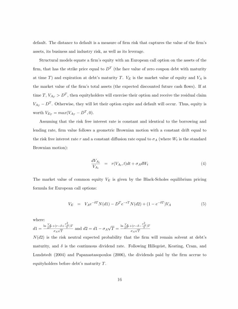
default. The distance to default is a measure of firm risk that captures the value of the firm’s

assets, its business and industry risk, as well as its leverage.

Structural models equate a firm’s equity with an European call option on the assets of the

firm, that has the strike price equal to DT (the face value of zero coupon debt with maturity

at time T ) and expiration at debt’s maturity T . VE is the market value of equity and VA is

the market value of the firm’s total assets (the expected discounted future cash flows). If at

time T , VAT> DT , then equityholders will exercise their option and receive the residual claim

VAT−DT . Otherwise, they will let their option expire and default will occur. Thus, equity is

worth VET= max(VAT

−DT , 0).

Assuming that the risk free interest rate is constant and identical to the borrowing and

lending rate, firm value follows a geometric Brownian motion with a constant drift equal to

the risk free interest rate r and a constant diffusion rate equal to σA (where Wt is the standard

Brownian motion):

dVAt

VAt

= r(VAt , t)dt + σAdWt (4)

The market value of common equity VE is given by the Black-Scholes equilibrium pricing

formula for European call options:

VE = VAe−δT N(d1)−DT e−rT N(d2) + (1− e−δT )VA (5)

where:

d1 =ln

VADT +(r−δ+

σ2A2

)T

σA

√T

and d2 = d1− σA

√T =

lnVADT +(r−δ−σ2

A2

)T

σA

√T

N(d2) is the risk neutral expected probability that the firm will remain solvent at debt’s

maturity, and δ is the continuous dividend rate. Following Hillegeist, Keating, Cram, and

Lundstedt (2004) and Papanastasopoulos (2006), the dividends paid by the firm accrue to

equityholders before debt’s maturity T .

16

The equation

σE = σAVA

VEN(d1)e−δT (6)

is derived from Ito’s lemma and shows the relationship between equity volatility and asset

volatility (equity-implied).

In order to estimate this model, I first compute equity volatility from historical returns for

each firm. To derive the equity-implied asset volatility and the value of firm’s assets, I solve the

system of two nonlinear equations with two unknowns ((5) and (6)) by using an optimization

procedure. In order to transform the results from risk-neutral to actual default probability, I

substitute the expected return on the firm asset value (µ) for the risk free interest rate. I use

the results to compute DD, the distance to default (which measures the number of standard

deviations that firm asset value is away from the default point), and EDP , the expected

default probability (equivalent to the probability that the option will expire unexercised):

DD =ln VA

DT + (µ− δ − σ2A2 )T

σA

√T

(7)

EDP = N(− ln VA

DT + (µ− δ − σ2A2 )T

σA

√T

) (8)

I calculate the market value of equity (VE) based on the average price in the month corre-

sponding to the firm’s fiscal year end. For the standard deviation of equity returns (σE), I use

daily return data from CRSP over the entire fiscal year. The maturity T equals one year and

the risk-free rate r is the one-year Treasury bill rate. Following Vassalou and Xing (2004) and

Papanastasopoulos (2006), the strike price X which is equal to the firm’s total liabilities, is

approximated with the sum of current liabilities (as previously defined) and half of long-term

liabilities (an assumption that is due to the one year maturity restriction). The dividend rate

17

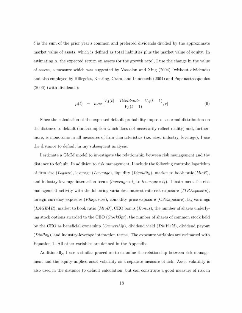
δ is the sum of the prior year’s common and preferred dividends divided by the approximate

market value of assets, which is defined as total liabilities plus the market value of equity. In

estimating µ, the expected return on assets (or the growth rate), I use the change in the value

of assets, a measure which was suggested by Vassalou and Xing (2004) (without dividends)

and also employed by Hillegeist, Keating, Cram, and Lundstedt (2004) and Papanastasopoulos

(2006) (with dividends):

µ(t) = max[VA(t) + Dividends− VA(t− 1)

VA(t− 1), r] (9)

Since the calculation of the expected default probability imposes a normal distribution on

the distance to default (an assumption which does not necessarily reflect reality) and, further-

more, is monotonic in all measures of firm characteristics (i.e. size, industry, leverage), I use

the distance to default in my subsequent analysis.

I estimate a GMM model to investigate the relationship between risk management and the

distance to default. In addition to risk management, I include the following controls: logarithm

of firm size (Logsize), leverage (Leverage), liquidity (Liquidity), market to book ratio(MtoB),

and industry-leverage interaction terms (leverage ∗ i1 to leverage ∗ i8). I instrument the risk

management activity with the following variables: interest rate risk exposure (ITRExposure),

foreign currency exposure (FExposure), comodity price exposure (CPExposure), lag earnings

(LAGEAR), market to book ratio (MtoB), CEO bonus (Bonus), the number of shares underly-

ing stock options awarded to the CEO (StockOpt), the number of shares of common stock held

by the CEO as beneficial ownership (Ownership), dividend yield (DivYield), dividend payout

(DivPay), and industry-leverage interaction terms. The exposure variables are estimated with

Equation 1. All other variables are defined in the Appendix.

Additionally, I use a similar procedure to examine the relationship between risk manage-

ment and the equity-implied asset volatility as a separate measure of risk. Asset volatility is

also used in the distance to default calculation, but can constitute a good measure of risk in

18

itself, since it captures the uncertainty of the asset value. Asset volatility is in fact a measure

of the firm’s business (in terms of size and nature) and industry risk.

4 Results

4.1 Duration Analysis Model Results

In this section I present the results of the cloglog model while controlling for the endogeneity

between risk management activity and the probability of default. I estimate GMM models,

where the instruments used for the risk management activity are lag earnings, interest rate

exposure, foreign currency exposure, commodity price exposure, bonus, stock options, man-

agerial stock ownership, dividend yield and dividend payout, all of which are defined in the

Appendix.

The results of the GMM estimation are shown in Table 45. The variable Any RM has a

negative coefficient and is significant at the 5% level. Since the magnitude of the regression

coefficient is not very informative, I calculate the exponential coefficient which is equal to

0.0364 and suggests that the odds of filing for bankruptcy (within the next year) of compa-

nies that use any type of risk management instruments is 3.6% of (or 96.4% lower than) the

odds of filing for bankruptcy of companies that do not manage risk. The magnitude of the

coefficient is quite high, a result which strongly supports the argument that risk management

helps extend a firm’s life. The coefficients on the variable indicating the use of a specific type

of risk management (interest rate, foreign currency, or commodity price) separately, are not

significantly related to the likelihood of bankruptcy, and thus no inference can be made about

their role in helping firms live longer.

Moving on to the control variables, the estimated coefficients indicate that, when FX RM is

5The exponential coefficients, indicating the odds of filing for bankruptcy, are not reported in Table 4, but availableupon request.

19

included in the regression, size has a strong negative impact on the probability of bankruptcy.

Thus, for this specification, larger firm size is associated with significantly lower odds of filing

for bankruptcy, a result which was also found by Altman, Haldeman, and Naraynan (1977),

Ohlson (1980), and Papanastasopoulos (2006). Similarly to the findings of Papanastasopou-

los (2006), more leverage in the capital structure is associated with a higher likelihood of

bankruptcy in the specifications that include Any RM and FX RM: the odds of going bankrupt

increases 10.4 times with a 1% increase in leverage, and 8.6 times respectively. Results also

indicate that there is no significant relationship between the odds of filing for bankruptcy and

liquidity or market to book ratio.

4.2 Option Pricing Model Results

4.2.1 Distance to Default

The distance to default generated with the Black-Scholes-Merton option pricing model has

a mean of 2.5 across all years, suggesting that, on average, the firms in the sample are 2.5

standard deviations away from default. Stated differently, on average, a firm would have to

incur a decrease of 2.5 standard deviations in its value of assets to default. The median is 1.8,

and the standard deviation is 2.9.

In order to investigate the relationship between the distance to default and risk manage-

ment, I estimate a GMM model that considers the possible endogeneity problem between the

two variables. Other controls (defined in the Appendix) used are: firm size, leverage, liquidity,

market to book ratio and interaction terms between firm industry and leverage. The results,

shown in Table 5, indicate that the coefficient on Any RM is positively and significant, indicat-

ing that any type of risk management activity is positively related to the distance to default,

and thus negatively related to the probability of bankruptcy. This suggests that, all else equal,

the number of standard deviations a company is away from default increases by approximately

3.2 units when that company manages any type of risk. As found in the previous test, the

20

magnitude of the coefficient is indicative of the importance of firms’ risk management activity

in reducing risk and extending a firm’s life. Interest rate risk management and foreign cur-

rency risk management are only weakly (significant at the 10% level) positively related to the

distance to default.

Moving on to the control variables, firm size is positively and significantly related to the

distance to default in three of the four specifications. Leverage is associated with a signifi-

cantly smaller distance to default in all specifications. However, liquidity is positively related

to the distance to default (i.e. a one percent increase in liquidity is associated with an increase

in the distance to default by approximately 2.8 units in the specification where Any RM is

included), and thus negatively related to the probability of bankruptcy in specifications that

include Any RM, IR RM, and FX RM. The market to book ratio is negatively and significantly

related to the distance to default in all specifications. Some interaction terms between firm

industry and leverage are also positively and significantly related to the distance to default.

4.2.2 Asset Volatility

Alternatively, I estimate a similar GMM model for the relationship between risk management

and the equity-implied asset volatility as a separate measure of firm risk.

The results, shown in Table 6, indicate that the coefficient on the risk management variable

in the specifications that include Any RM, IR RM, and FX RM is negative and significant (at

the 5% level) related to asset volatility. They suggest that a firm’s asset volatility decreases

by 64% when it uses any risk management instruments, by 99% when it uses interest rate

risk management instruments, and by 60% when it uses foreign currency risk management

instruments. These results are indicative of the important contribution of risk management in

mitigating firms’ business risk.

As far as the firm-specific covariates are concerned, size is the only one that is significantly

related to asset volatility. Given the negative relationship, larger firms tend to have lower asset

21

volatility and thus to default less, result which agrees with the previous findings.

5 Robustness checks

5.1 Changes in Firm’s Risk Management Activity

As a first robustness check, I investigate the effect of changes in firms’ risk management activi-

ties on the changes in the distance to default and asset volatility. More specifically, I calculate

the difference from one year to another in the risk management activity (+1, 0, -1), as well

as in the distance to default, asset volatility, and all other controls. Real changes in the risk

management activity (i.e. +1 or -1) are not very common in this sample, most companies

remaining true to their historical risk management activity. This agrees with the prediction

from Fehle and Tsyplakov (2005) that firms that are deep in financial distress neither initiate

nor adjust their risk management practices.

Distance to Default

In order to investigate the relationship between the change in the risk management activity

and the change in the model-implied distance to default, I estimate the GMM model as previ-

ously described in Subsection 3.2.2 in first differences, i.e. all variables are changes relative to

the previous year. The results are shown in Table 7. The coefficient on the change in the risk

management variable is significant (at the 1% or 5% level) in each specification. For the spec-

ifications that include Any RM, IR RM, and FX RM, risk management is positively related

to the change in the distance to default thus suggesting a reduction in the risk of default. For

the CP RM specification, risk management activity is negatively related to the change in the

distance to default, contrary to the risk-reduction hypothesis.

22

Asset Volatility

The relationship between the change in the risk management activity and the change in

asset volatility, estimated using GMM, is presented in Table 8. The change in any risk man-

agement activity is negatively and significantly (at the 5% level) related to the change in asset

volatility. Therefore, an increase in firm’s risk management activity is associated with a de-

crease in its asset volatility. Similarly, the change in interest rate risk management activity is

negatively related to the change in asset volatility, but only at the 10% level.

5.2 Sub-sample Analysis: Exposure

In this subsection, I present the results of the GMM estimation described in Subsection 3.2.2 for

both the relationship between risk management and the distance to default and between risk

management and the equity-implied asset volatility on a series of sub-samples with different

risk exposure. This analysis is meant to provide insights on whether firms’ risk management

activities are driven by their hedging needs (as measured by their risk exposure), and to

examine whether the relationships found previously still hold.

I first calculate the mean interest rate exposure, foreign currency exposure, and commodity

price exposure using Equation 1 for the entire sample. Then I divide the sample into two sub-

samples: firms with a particular exposure lower than the mean and higher than the mean

respectively. Thus, I analyze six different sub-samples, and estimate GMM as before for each

sub-sample.

5.2.1 Interest Rate Exposure

The sub-sample of firms with interest rate exposure lower than the sample mean is comprised

of 59.6% bankrupt and 40.4% non-bankrupt firms. Across all years, 41.6% use any type of risk

management instruments, 18.1% use interest rate risk management instruments, 32.5% use

23

foreign currency risk management instruments, and 6% use commodity price risk management

instruments.

On the other hand, there are 48.7% bankrupt and 51.3% non-bankrupt firms in the sub-

sample of firms with interest rate exposure higher than the mean. 52.5% of the firms use any

type of risk management instruments, 28.8% use interest rate risk management instruments,

32.4% use foreign currency risk management instruments, and 10.4% use commodity price risk

management instruments. A simple comparison suggests that the firms in the sub-sample with

high interest rate exposure tend to make greater use of risk management instruments than the

firms in the sub-sample with low interest-rate exposure. The regression results (as detailed

below) for the sub-sample of firms with high interest exposure reinforce the main result that

an increase in the risk management activity is associated with a higher distance to default, and

a lower asset volatility. However, the result is not present in the sub-sample of firms with low

interest rate exposure, which could be explained by the fact that a low interest rate exposure

is equivalent to low hedging needs (possibly due to the past risk management activity).

Distance to Default

The results of the GMM estimation for the relationship between risk management and

the distance to default are presented in Table 9, separately for the two sub-samples of firms

with interest rate exposure lower and higher than the mean. In the case of the firms with

high interest rate exposure, a 1% increase in Any RM augments the distance to default by

4.5 units (significant at the 5% level). Similarly, a 1% increase in CP RM augments the

distance to default by 4.6 units, but this result is only weakly significant (at the 10% level).

On the other hand, for firms with interest rate exposure lower than the mean, a 1% increase in

CP RM reduces the distance to default by 6.4 units. The negative relationship found between

commodity price risk management and the distance to default indicates that, when interest

rate hedging needs are low, the use of commodity price risk management instruments is unlikely

24

to benefit the firm and may in fact be harmful. Therefore, risk management instruments are

associated with an increase in firms’ distance to default and a decrease in their asset volatility

if used according to their hedging needs (measured by the interest rate exposure).

Asset Volatility

Table 10 shows the results of the GMM estimation between risk management and asset

volatility, for the two sub-samples of firms with interest rate exposure lower and higher than

the mean. While no relationship can be found for the firms with low interest rate exposure, in

the case of firms with high interest rate exposure, IR RM, FX RM and CP RM are negatively

and significantly (at the 10%, 1% and the 5% level, respectively) related to asset volatility.

5.2.2 Foreign Currency Exposure

In the sub-sample of firms with foreign currency exposure lower than the sample mean there

are 55.4% bankrupt and 44.6% non-bankrupt firms. Across all years, the percentages of firms

using any type of risk management instruments, interest rate risk management instruments,

foreign currency risk management instruments, commodity price risk management instruments

are 48.8%, 25.9%, 30.1%, and 9.2% respectively.

The sub-sample of firms with foreign currency exposure higher than the mean is composed

of 46.9% bankrupt and 53.1% non-bankrupt firms. In this sub-sample, the percentages of firms

using any type of risk management instruments, interest rate risk management instruments,

foreign currency risk management instruments, commodity price risk management instruments

are 50.2%, 25.5%, 35.8%, and 9% respectively. The regression results, detailed below, are simi-

lar to the ones found for the sub-samples of firms with high and low interest rate exposure, and

suggest that risk management instruments are associated with an increase in firms’ distance

to default and a decrease in their asset volatility if used according to their hedging needs (as

measured by the foreign currency exposure).

25

Distance to Default

Table 11 presents the results of the GMM estimation between risk management and the

distance to default, separately for the two sub-samples of firms with foreign currency exposure

lower and higher than the mean. In the case of firms with high foreign currency exposure,

Any RM, IR RM, and FX RM are positively and significantly related to the distance to de-

fault. For example a 1% increase in Any RM augments the distance to default by 5.3 units.

CP RM is also positively related to the distance to default, but significant only at the 10%

level. On the other hand, in the case of firms with low foreign currency exposure, CP RM is

weakly negatively related to the distance to default (significant at the 10% level), result which

is similar to the one in the sample of firms with low interest rate exposure. The other three

specifications are not significantly related to the distance to default in the case of firms with

low foreign currency exposure.

Asset Volatility

The results of the GMM estimation between risk management and asset volatility, sepa-

rately for the two sub-samples of firms with foreign currency exposure lower and higher than

the mean, are shown in Table 12. Any RM is negatively associated to asset volatility only

in the case of firms with low foreign currency exposure, indicating that a 1% increase in risk

management decreases asset volatility by 59%. IR RM is negatively and significantly related to

asset volatility in both sub-samples. Similarly, FX RM is negatively related to asset volatility

for both the case of firms with high and low foreign currency exposure, but significant only

at the 10% level. Weak significance is also found for the relationship between CP RM and

asset volatility in the sub-sample with high foreign currency exposure; no relationship can be

observed in the sub-sample with low foreign currency exposure.

26

5.2.3 Commodity Price Exposure

In the sub-sample of firms with foreign currency exposure lower than the sample mean, there

are 55.2% bankrupt and 44.8% non-bankrupt firms. Across all years, 50% use any type of risk

management instruments, 26.5% use interest rate risk management instruments, 35.4% use

foreign currency risk management instruments, and 7.3% use commodity price risk manage-

ment instruments.

As for the sub-sample of firms with foreign currency exposure higher than the mean, 47.4%

of the firms are bankrupt and 52.6% are non-bankrupt. 48.6%, 24.7%, 28.7%, and 11.6%

of these firms use any type of risk management instruments, interest rate risk management

instruments, foreign currency risk management instruments, and commodity price risk man-

agement instruments. Opposite to the regression results from the sub-samples of firms with

high/low interest rate exposure and foreign currency exposure, in these sub-samples evidence

indicates that the use of risk management instruments is mainly associated with an increase

in the distance to default and a decrease in asset volatility for the firms with low commodity

price exposure. Therefore, the uses of any type risk management instruments, interest rate

risk management, and foreign currency risk management, which are related to an increase in

the distance to default and to a decrease in asset volatility, are not likely to be driven by firms’

commodity price hedging needs.

Distance to Default

For the two sub-samples of firms with commodity price exposure lower and higher than the

mean, the results of the GMM estimation for the relationship between risk management and

the distance to default are presented in Table 13. While for the firms with high commodity

price exposure, no relationship can be found between the risk management activity and the

distance to default, in the case of firms with low commodity price exposure there is a positive

and significant relationship for the Any RM, IR RM, and FX RM specifications. For example,

27

a 1% increase in any risk management activity augments the distance to default by approxi-

mately 3 units.

Asset Volatility

Table 14 shows the results of the GMM estimation between risk management and asset

volatility, separately for the two sub-samples of firms with commodity price exposure lower

and higher than the mean. Any RM and FX RM are negatively related to asset volatility

for the firms with low commodity price exposure. IR RM is also negatively related to asset

volatility for both firms with high and low commodity price exposure.

5.3 Sub-sample Analysis: Bankrupt and Non-Bankrupt

Lastly, another robustness check consists of separating the sample into sub-samples of bankrupt

and non-bankrupt firms, and estimating GMM in order to examine the relationship between

risk management and the distance to default or asset volatility. This analysis examines whether

the bankrupt and/or the non-bankrupt firms show specific patterns with respect to their risk

management activities.

As mentioned before, the characteristics of each group are shown in Table 3. The regres-

sion results support the main finding on the relationship between risk management and asset

volatility in both sub-samples, with not much evidence on the relationship between risk man-

agement and the distance to default.

Distance to Default

The results of the GMM estimation between risk management and the distance to default,

separately for the two sub-samples of bankrupt and nonbankrupt firms, are presented in Table

15. The variable IR RM is the only one that has a negative coefficient which is only significant

28

at the 10% level in the sub-sample of nonbankrupt firms. It suggests that, for companies

that use interest rate risk management instruments, the number of standard deviations the

asset value is away from the default point decreases by 1 unit, all else equal. This result

does not supports the hypothesis that interest rate risk management reduces the probability

of bankruptcy in this sub-sample. All other risk management variables are not statistically

significant. No inference can be made about the relationship between the risk management

activity and the distance to default in the sub-sample of bankrupt firms.

Asset Volatility

Unlike the distance to default, asset volatility has a significant relationship with the risk

management variables for the two sub-samples of bankrupt and nonbankrupt firms, as shown

in Table 16. Any RM is negatively and significantly related to asset volatility for the sub-

sample of bankrupt firms. IR RM and FX RM are also negatively and significantly related

to asset volatility for both sub-samples. For example, a 1% increase in the interest rate risk

management reduces asset volatility by 68%.

6 Conclusion

This paper examines whether the use of risk management instruments for a sample of bankrupt

and non-bankrupt firms impacts firms’ riskiness in terms of their probability of bankruptcy,

distance to default, and asset volatility. To my knowledge, the latter two measures of firm risk

have not been used in the prior literature on risk management, while the former has not been

used in the context of duration analysis.

In a framework that controls for the endogeneity between risk management and the prob-

ability of default, this paper provides evidence that the risk management activity contributes

29

to a lower probability of bankruptcy, higher distance to default, and lower asset volatility, all

of which suggest risk reduction and consequently a longer life for the firm. Both approaches

presented in this paper (duration analysis approach and option approach) show strong support

with respect to the role of risk management in general and provide some evidence with respect

to individual types of risk management: interest rate, foreign currency, and commodity price

risk management. Sub-sample analysis generally confirms the main results and brings some

insights with respect to the use of different types of risk management instruments depending

on the firms’ risk exposure (or hedging needs). For example, evidence indicates that the benefit

of using risk management instruments is greater when firms’ interest rate and foreign currency

hedging needs are high, and commodity price hedging needs are low. Overall, for firms with

high interest rate exposure and foreign currency exposure, as well as with low commodity

price exposure, the use of risk management instruments is associated with a higher distance to

default and a lower asset volatility. However, for companies with low interest rate and foreign

currency exposure, the use of commodity price risk management is negatively related to the

distance default. Similarly, the changes in commodity price risk management are negatively

related to the changes in the distance to default, suggesting that the initiations of commodity

price risk management actually reduce firms’ distance to default. The answer to the question

on whether firms with lower overall risk exposure are less likely to use commodity price risk

management instruments for risk-reduction purposes is left for future research.

30

References

Adam, Tim R., 2002, Do Firms Use Derivatives to Reduce their Dependence on External CapitalMarkets?, European Finance Review pp. 163–187.

Altman, E., R. Haldeman, and P. Naraynan, 1977, ZETA Analysis: A New Model to IdentifyBankruptcy Prediction Risk of Corporations, .

Altman, Edward I., 1968, Financial ratios, discriminant analysis and the prediction of corporatebankruptcy, Journal of Finance 23, 589–609.

, 1973, Predicting Railroad Bankruptcies in America, Bell Journal of Economics and Manage-ment Science 3, 184–211.

Beaver, W. H., 1966, Financial Ratios as Predictors of Failure, Journal of Accounting Research (Sup-plement) pp. 71–102.

Black, Fischer, and Myron Scholes, 1973, The pricing of options and corporate liabilities, Journal ofPolitical Economy 81, 637–659.

Charitou, A., N. Lambertides, and L. Trigeorgis, 2004, Is the Impact of Default Risk Systematic? AnOption-Pricing Explanation, Working Paper, University of Cyprus.

Charitou, Andreas, and Leon Trigeorgis, 2002, Option-based Bankruptcy Prediction, Working Paper,University of Cyprus.

Delianedis, R., and R. Geske, 1999, Credit Risk and Risk Neutral Probabilities: Information aboutRating Migrations and Defaults, UCLA Working Paper.

Faulkender, Michael, 2005, Hedging or market timing? Selecting the interest rate exposure of corporatedebt, Journal of Finance 60, 931–962.

Fehle, Frank, and Sergey Tsyplakov, 2005, Dynamic Risk Management: Theory and Evidence, Journalof Financial Economics.

Fok, R. C. W., C. Carroll, and M. C. Chiou, 1997, Determinants of corporate hedging and derivatives:a revisit, Journal of Economics and Business 49, 569–585.

Froot, Kenneth A., David S. Scharfstein, and Jeremy C. Stein, 1993, Risk Management: CoordinatingCorporate Investment and Financing Policies, Journal of Finance 48, 1629–1658.

Graham, John R., and Clifford Jr. Smith, 1999, Tax Incentives to Hedge, The Journal of Finance 54,2241–2262.

Hillegeist, Stephen A., Elizabeth K. Keating, Donald P. Cram, and Kyle G. Lundstedt, 2004, Assessingthe Probability of Bankruptcy, Review of Accounting Studies 9, 5–34.

Judge, Amrit, 2003, Why and How UK Firms Hedge, European Financial Management Journal 12.

Kedia, S., and A. Mozumdar, 2003, Foreign currency denominated debt: an empirical investigation,Journal of Business 76, 521–546.

Merton, C. R., 1974, On the Pricing of Corporate Debt: The Risk Structure of Interest Rates, Journalof Finance 29, 449–470.

Mian, Shehzad, 1996, Evidence on Corporate Hedging Policy, The Journal of Financial and QuantitativeAnalysis 11, 419–439.

Nance, Deana R., Clifford W. Smith, and Charles W. Smithson, 1993, On the Determinants of CorporateHedging, The Journal of Finance 48, 267–284.

31

Ohlson, James A., 1980, Financial Ratios and the Probabilistic Prediction of Bankruptcy, Journal ofAccounting Research 18, 109–131.

Papanastasopoulos, George, 2006, Using Option Theory and Fundamentals to Assessing Default Riskof Listed Firms, Working Paper, University of Peloponnese.

Purnanandam, Amiyatosh, 2007, Financial Distress and Corporate Risk Management: Theory & Evi-dence, Journal of Financial Economics, forthcoming.

Rogers, Daniel A., 2002, Does Executive Portfolio Structure Affect Risk Management? CEO Risk-taking Incentives and Corporate Derivative Usage, Journal of Banking and Finance 26, 271–296.

Shumway, Tyler, 2001, Forecasting Bankruptcy More Accurately: A Simple Hazard Model, The Journalof Business 74, 101–124.

Smith, Clifford W., and Rene M. Stulz, 1985, The Determinants of Firms’ Hedging Policies, The Journalof Financial and Quantitative Analysis 20, 391–405.

Tufano, Peter, 1996, Who Manages Risk? An Empirical Examination of Risk Management Practicesin the Gold Mining Industry, Journal of Finance 51, 1097–1137.

Vassalou, Maria, and Yuhang Xing, 2004, Default Risk in Equity Returns, The Journal of Finance 49,831–868.

Zmijewski, Mark E., 1984, Methodological Issues Related to the Estimation of Financial Distress Pre-diction Models, Studies on Current Econometric Issues in Accounting Research.

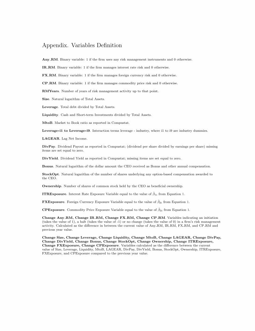
Appendix. Variables Definition

Any RM. Binary variable: 1 if the firm uses any risk management instruments and 0 otherwise.

IR RM. Binary variable: 1 if the firm manages interest rate risk and 0 otherwise.

FX RM. Binary variable: 1 if the firm manages foreign currency risk and 0 otherwise.

CP RM. Binary variable: 1 if the firm manages commodity price risk and 0 otherwise.

RMYears. Number of years of risk management activity up to that point.

Size. Natural logarithm of Total Assets.

Leverage. Total debt divided by Total Assets.

Liquidity. Cash and Short-term Investments divided by Total Assets.

MtoB. Market to Book ratio as reported in Compustat.

Leverage∗i1 to Leverage∗i9. Interaction terms leverage - industry, where i1 to i9 are industry dummies.

LAGEAR. Lag Net Income.

DivPay. Dividend Payout as reported in Compustat; (dividend per share divided by earnings per share) missingitems are set equal to zero.

DivYield. Dividend Yield as reported in Compustat; missing items are set equal to zero.

Bonus. Natural logarithm of the dollar amount the CEO received as Bonus and other annual compensation.

StockOpt. Natural logarithm of the number of shares underlying any option-based compensation awarded tothe CEO.

Ownership. Number of shares of common stock held by the CEO as beneficial ownership.

ITRExposure. Interest Rate Exposure Variable equal to the value of β1i from Equation 1.

FXExposure. Foreign Currency Exposure Variable equal to the value of β2i from Equation 1.

CPExposure. Commodity Price Exposure Variable equal to the value of β3i from Equation 1.

Change Any RM, Change IR RM, Change FX RM, Change CP RM. Variables indicating an initiation(takes the value of 1), a halt (takes the value of -1) or no change (takes the value of 0) in a firm’s risk managementactivity. Calculated as the difference in between the current value of Any RM, IR RM, FX RM, and CP RM andprevious year value.

Change Size, Change Leverage, Change Liquidity, Change MtoB, Change LAGEAR, Change DivPay,Change DivYield, Change Bonus, Change StockOpt, Change Ownership, Change ITRExposure,Change FXExposure, Change CPExposure. Variables calculated as the difference between the currentvalue of Size, Leverage, Liquidity, MtoB, LAGEAR, DivPay, DivYield, Bonus, StockOpt, Ownership, ITRExposure,FXExposure, and CPExposure compared to the previous year value.

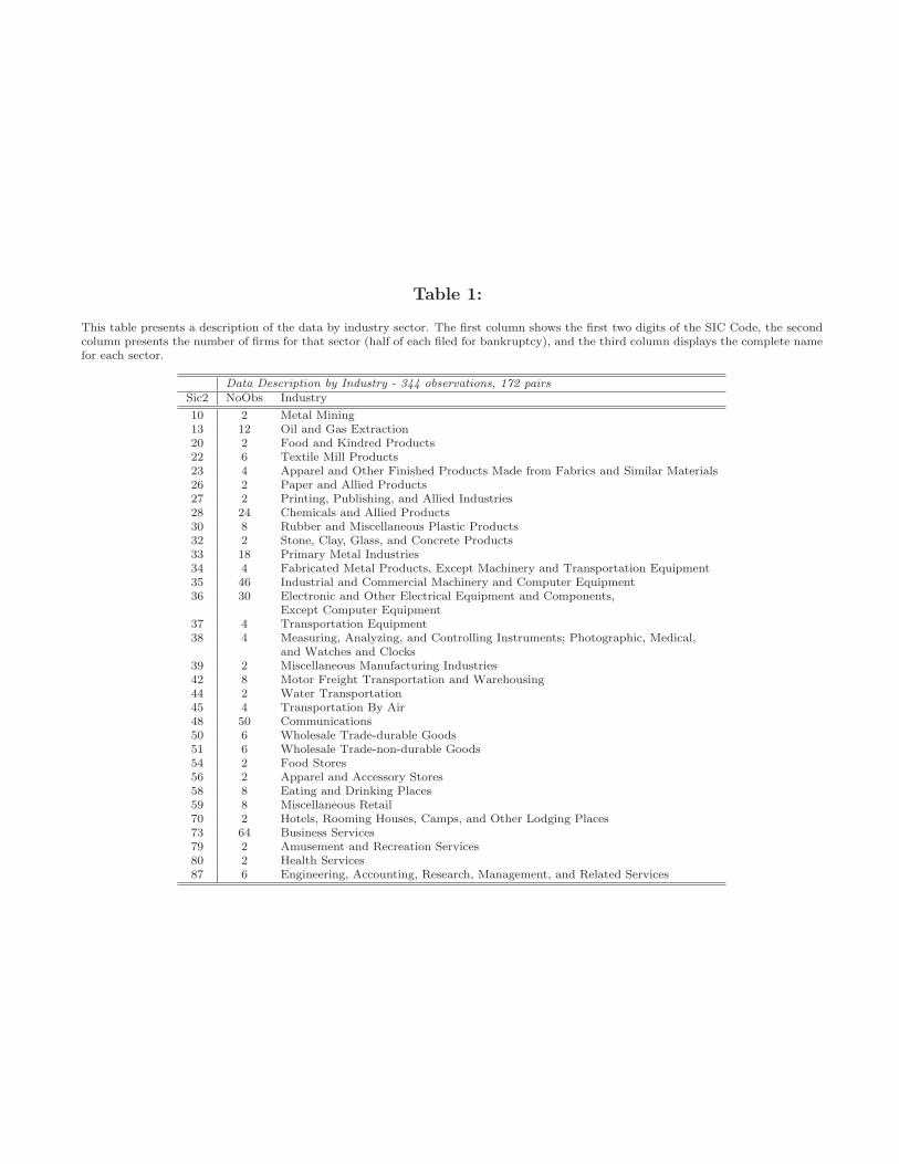
Table 1:

This table presents a description of the data by industry sector. The first column shows the first two digits of the SIC Code, the secondcolumn presents the number of firms for that sector (half of each filed for bankruptcy), and the third column displays the complete namefor each sector.

Data Description by Industry - 344 observations, 172 pairsSic2 NoObs Industry

10 2 Metal Mining13 12 Oil and Gas Extraction20 2 Food and Kindred Products22 6 Textile Mill Products23 4 Apparel and Other Finished Products Made from Fabrics and Similar Materials26 2 Paper and Allied Products27 2 Printing, Publishing, and Allied Industries28 24 Chemicals and Allied Products30 8 Rubber and Miscellaneous Plastic Products32 2 Stone, Clay, Glass, and Concrete Products33 18 Primary Metal Industries34 4 Fabricated Metal Products, Except Machinery and Transportation Equipment35 46 Industrial and Commercial Machinery and Computer Equipment36 30 Electronic and Other Electrical Equipment and Components,

Except Computer Equipment37 4 Transportation Equipment38 4 Measuring, Analyzing, and Controlling Instruments; Photographic, Medical,

and Watches and Clocks39 2 Miscellaneous Manufacturing Industries42 8 Motor Freight Transportation and Warehousing44 2 Water Transportation45 4 Transportation By Air48 50 Communications50 6 Wholesale Trade-durable Goods51 6 Wholesale Trade-non-durable Goods54 2 Food Stores56 2 Apparel and Accessory Stores58 8 Eating and Drinking Places59 8 Miscellaneous Retail70 2 Hotels, Rooming Houses, Camps, and Other Lodging Places73 64 Business Services79 2 Amusement and Recreation Services80 2 Health Services87 6 Engineering, Accounting, Research, Management, and Related Services

Table 2:

This table presents a year-by-year description of the data. The second column shows the number of bankruptcies that were filed eachfiscal year, while the third column identifies the number of observations in the sample for each fiscal year.

Data Description by Year:Year # Bankruptcy Filings # Observations in the Sample

1994 101995 121996 201997 461998 4 1221999 11 1782000 20 2262001 46 1742002 41 942003 29 422004 20 22005 1Total 172 926

Table 3:

This table presents summary statistics (mean and standard deviation) of firm characteristics for companies that filed for bankruptcyand the control group, for the fiscal year before bankruptcy filing. The variables shown are: any risk management (Any RM), interestrate risk management (IR RM), foreign exchange risk management (FX RM), commodity price risk management (CP RM), size (Size),leverage (Leverage), and liquidity (Liquidity). These are defined in Appendix.

Characteristic Bankrupt Firms (172) Control Group (172)Mean Std.Dev. Mean Std. Dev

Any RM 43.02% .49 51.74% .50IR RM 25.00% .43 27.90% .45FX RM 20.34% .40 30.23% .46CP RM 9.88% .29 5.81% .23

Size $1,239,120 $8,123,232 $1,180,896 $7,541.997Leverage 56.45% .57 29.76% .31Liquidity 13.77% .19 23.18% .26

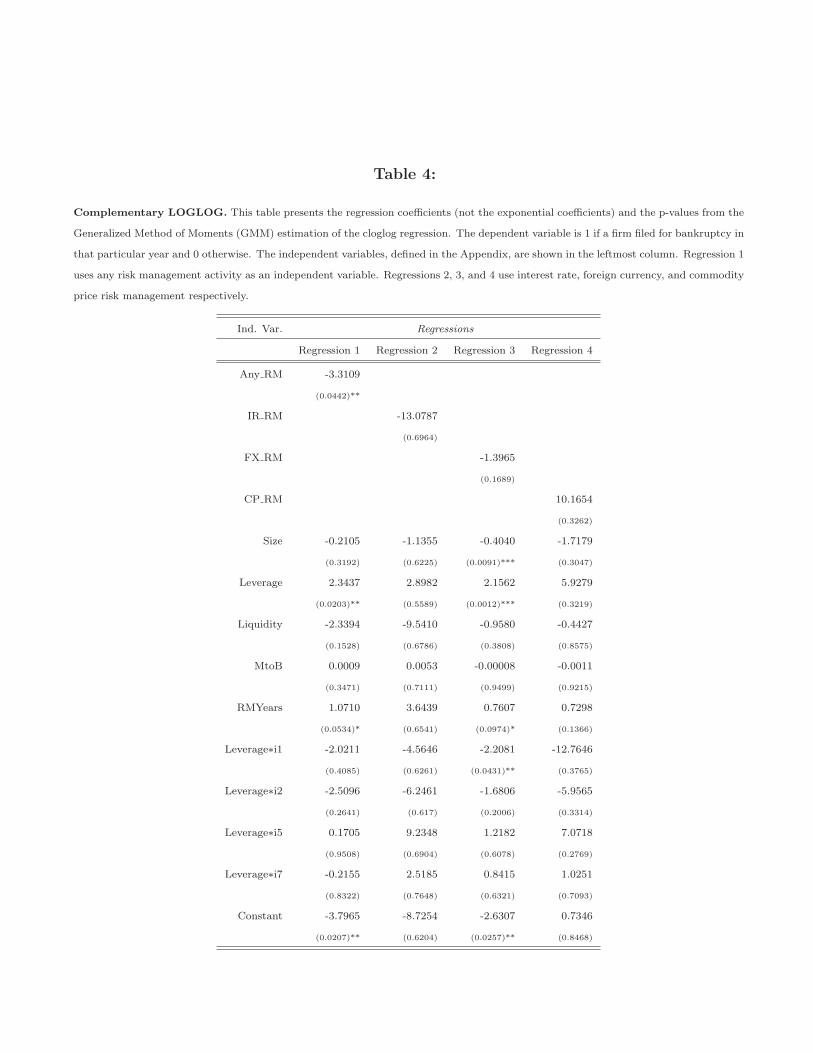
Table 4:

Complementary LOGLOG. This table presents the regression coefficients (not the exponential coefficients) and the p-values from the

Generalized Method of Moments (GMM) estimation of the cloglog regression. The dependent variable is 1 if a firm filed for bankruptcy in

that particular year and 0 otherwise. The independent variables, defined in the Appendix, are shown in the leftmost column. Regression 1

uses any risk management activity as an independent variable. Regressions 2, 3, and 4 use interest rate, foreign currency, and commodity

price risk management respectively.

Ind. Var. Regressions

Regression 1 Regression 2 Regression 3 Regression 4

Any RM -3.3109

(0.0442)**

IR RM -13.0787

(0.6964)

FX RM -1.3965

(0.1689)

CP RM 10.1654

(0.3262)

Size -0.2105 -1.1355 -0.4040 -1.7179

(0.3192) (0.6225) (0.0091)*** (0.3047)

Leverage 2.3437 2.8982 2.1562 5.9279

(0.0203)** (0.5589) (0.0012)*** (0.3219)

Liquidity -2.3394 -9.5410 -0.9580 -0.4427

(0.1528) (0.6786) (0.3808) (0.8575)

MtoB 0.0009 0.0053 -0.00008 -0.0011

(0.3471) (0.7111) (0.9499) (0.9215)

RMYears 1.0710 3.6439 0.7607 0.7298

(0.0534)* (0.6541) (0.0974)* (0.1366)

Leverage∗i1 -2.0211 -4.5646 -2.2081 -12.7646

(0.4085) (0.6261) (0.0431)** (0.3765)

Leverage∗i2 -2.5096 -6.2461 -1.6806 -5.9565

(0.2641) (0.617) (0.2006) (0.3314)

Leverage∗i5 0.1705 9.2348 1.2182 7.0718

(0.9508) (0.6904) (0.6078) (0.2769)

Leverage∗i7 -0.2155 2.5185 0.8415 1.0251

(0.8322) (0.7648) (0.6321) (0.7093)

Constant -3.7965 -8.7254 -2.6307 0.7346

(0.0207)** (0.6204) (0.0257)** (0.8468)

Table 5:

Distance to Default. This table presents the regression coefficients and the p-values from the Generalized Method of Moments (GMM)

estimation of the relationship between the distance to default on one side and risk management activity, firm-specific covariates, and

industry - leverage interaction terms on the other side. The dependent variable is the distance to default calculated with the Black-

Scholes-Merton model. The independent variables, defined in the Appendix, are shown in the leftmost column. Regression 1 uses the any

risk management activity as an independent variable. Regressions 2, 3, and 4 use interest rate, foreign currency, and commodity price

risk management respectively.

Ind. Var. Regressions

Regression 1 Regression 2 Regression 3 Regression 4

Any RM 3.1990

(0.0227)**

IR RM 3.4447

(0.0646)*

FX RM 2.5520

(0.0785)*

CP RM -3.3579

(0.3218)

Size 0.3478 0.4780 0.4464 0.9422

(0.0686)* (0.0015)*** (0.0191)** (0.0001)***

Leverage -5.3667 -7.1865 -4.5738 -7.4293

(<.0001)*** (<.0001)*** (<.0001)*** (<.0001)***

Liquidity 2.8580 1.8096 2.5796 0.7734

(0.0073)*** (0.0207)** (0.0107)** (0.3775)

MtoB -0.0090 -0.0071 -0.0080 -0.0065

(0.0001)*** (<.0001)*** (<.0001)*** (0.0213)**

Leverage∗i1 3.1835 5.1260 3.7848 5.0298

(0.0045)*** (0.0054)*** (0.0145)** (0.078)*

Leverage∗i2 6.4726 6.8362 5.1384 5.1242

(0.0002)*** (0.0001)*** (0.0008)*** (0.0003)***

Leverage∗5 6.2212 3.0604 5.9247 -0.0307

(0.2355) (0.5958) (0.2147) (0.9935)

Leverage∗i7 4.0905 5.1971 3.0287 -6.8459

(0.0003)*** (0.0013)*** (0.0067)*** (0.2165)

Constant -0.6463 0.2460 -0.6682 -0.5369

(0.434) (0.7145) (0.3965) (0.572)

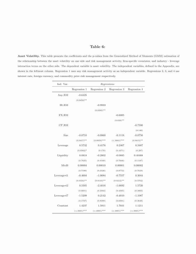
Table 6:

Asset Volatility. This table presents the coefficients and the p-values from the Generalized Method of Moments (GMM) estimation of

the relationship between the asset volatility on one side and risk management activity, firm-specific covariates, and industry - leverage

interaction terms on the other side. The dependent variable is asset volatility. The independent variables, defined in the Appendix, are

shown in the leftmost column. Regression 1 uses any risk management activity as an independent variable. Regressions 2, 3, and 4 use

interest rate, foreign currency, and commodity price risk management respectively.

Ind. Var. Regressions

Regression 1 Regression 2 Regression 3 Regression 4

Any RM -0.6425

(0.0459)**

IR RM -0.9933

(0.0282)**

FX RM -0.6005

(0.039)**

CP RM -0.7590

(0.146)

Size -0.0710 -0.0860 -0.1118 -0.0756

(0.0417)** (0.0059)*** (<.0001)*** (0.0415)**

Leverage 0.5732 0.4176 0.2467 0.3487

(0.0582)* (0.176) (0.4471) (0.287)

Liquidity 0.0818 -0.2802 -0.0885 0.40468

(0.7625) (0.4168) (0.7848) (0.1187)

MtoB 0.00004 0.00010 0.00001 0.00002

(0.7199) (0.2326) (0.8772) (0.7629)

Leverage∗i1 -0.4604 -1.0084 -0.7557 0.3044

(0.0434)** (0.0143)** (0.0212)** (0.5762)

Leverage∗i2 0.5505 -2.4016 -1.6692 1.5720

(0.6851) (0.2492) (0.4365) (0.3865)

Leverage∗i7 -1.5209 0.2142 -0.4010 -1.1087

(0.1727) (0.8399) (0.6991) (0.3648)

Constant 1.4237 1.5911 1.7031 1.1211

(<.0001)*** (<.0001)*** (<.0001)*** (<.0001)***

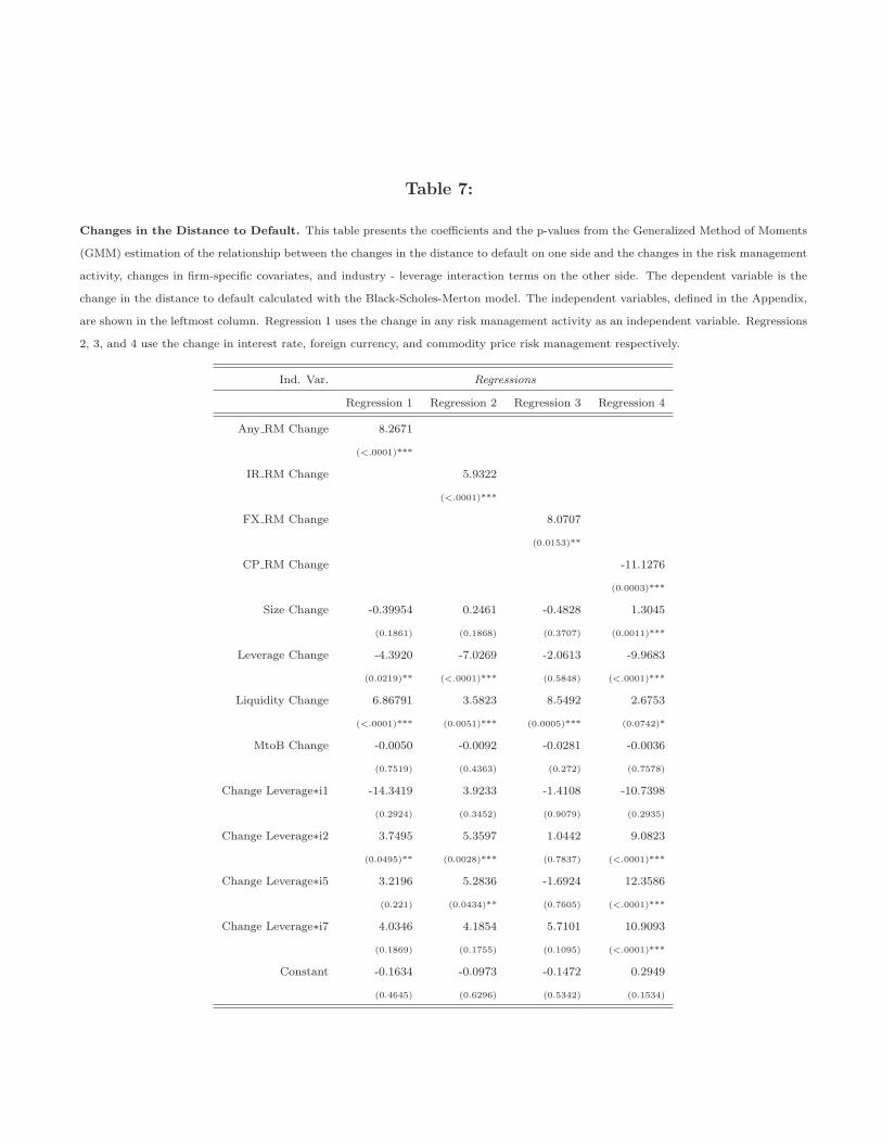
Table 7:

Changes in the Distance to Default. This table presents the coefficients and the p-values from the Generalized Method of Moments

(GMM) estimation of the relationship between the changes in the distance to default on one side and the changes in the risk management

activity, changes in firm-specific covariates, and industry - leverage interaction terms on the other side. The dependent variable is the

change in the distance to default calculated with the Black-Scholes-Merton model. The independent variables, defined in the Appendix,

are shown in the leftmost column. Regression 1 uses the change in any risk management activity as an independent variable. Regressions

2, 3, and 4 use the change in interest rate, foreign currency, and commodity price risk management respectively.

Ind. Var. Regressions

Regression 1 Regression 2 Regression 3 Regression 4

Any RM Change 8.2671

(<.0001)***

IR RM Change 5.9322

(<.0001)***

FX RM Change 8.0707

(0.0153)**

CP RM Change -11.1276

(0.0003)***

Size Change -0.39954 0.2461 -0.4828 1.3045

(0.1861) (0.1868) (0.3707) (0.0011)***

Leverage Change -4.3920 -7.0269 -2.0613 -9.9683

(0.0219)** (<.0001)*** (0.5848) (<.0001)***

Liquidity Change 6.86791 3.5823 8.5492 2.6753

(<.0001)*** (0.0051)*** (0.0005)*** (0.0742)*

MtoB Change -0.0050 -0.0092 -0.0281 -0.0036

(0.7519) (0.4363) (0.272) (0.7578)

Change Leverage∗i1 -14.3419 3.9233 -1.4108 -10.7398

(0.2924) (0.3452) (0.9079) (0.2935)

Change Leverage∗i2 3.7495 5.3597 1.0442 9.0823

(0.0495)** (0.0028)*** (0.7837) (<.0001)***

Change Leverage∗i5 3.2196 5.2836 -1.6924 12.3586

(0.221) (0.0434)** (0.7605) (<.0001)***

Change Leverage∗i7 4.0346 4.1854 5.7101 10.9093

(0.1869) (0.1755) (0.1095) (<.0001)***

Constant -0.1634 -0.0973 -0.1472 0.2949

(0.4645) (0.6296) (0.5342) (0.1534)

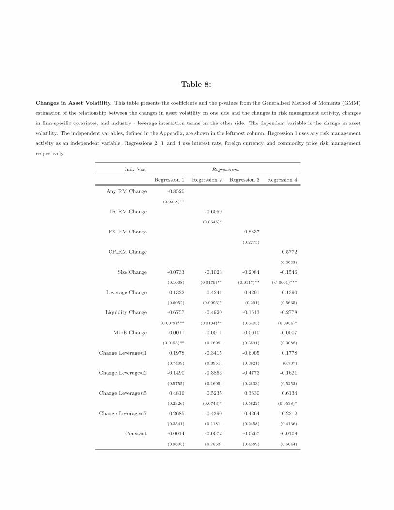
Table 8:

Changes in Asset Volatility. This table presents the coefficients and the p-values from the Generalized Method of Moments (GMM)

estimation of the relationship between the changes in asset volatility on one side and the changes in risk management activity, changes

in firm-specific covariates, and industry - leverage interaction terms on the other side. The dependent variable is the change in asset

volatility. The independent variables, defined in the Appendix, are shown in the leftmost column. Regression 1 uses any risk management

activity as an independent variable. Regressions 2, 3, and 4 use interest rate, foreign currency, and commodity price risk management

respectively.

Ind. Var. Regressions

Regression 1 Regression 2 Regression 3 Regression 4

Any RM Change -0.8520

(0.0378)**

IR RM Change -0.6059

(0.0645)*

FX RM Change 0.8837

(0.2275)

CP RM Change 0.5772

(0.2022)

Size Change -0.0733 -0.1023 -0.2084 -0.1546

(0.1008) (0.0179)** (0.0117)** (<.0001)***

Leverage Change 0.1322 0.4241 0.4291 0.1390

(0.6052) (0.0996)* (0.291) (0.5635)

Liquidity Change -0.6757 -0.4920 -0.1613 -0.2778

(0.0079)*** (0.0134)** (0.5403) (0.0954)*

MtoB Change -0.0011 -0.0011 -0.0010 -0.0007

(0.0155)** (0.1699) (0.3591) (0.3088)

Change Leverage∗i1 0.1978 -0.3415 -0.6005 0.1778

(0.7409) (0.3951) (0.3921) (0.737)

Change Leverage∗i2 -0.1490 -0.3863 -0.4773 -0.1621

(0.5755) (0.1605) (0.2833) (0.5252)

Change Leverage∗i5 0.4816 0.5235 0.3630 0.6134

(0.2326) (0.0743)* (0.5622) (0.0538)*

Change Leverage∗i7 -0.2685 -0.4390 -0.4264 -0.2212

(0.3541) (0.1181) (0.2458) (0.4136)

Constant -0.0014 -0.0072 -0.0267 -0.0109

(0.9605) (0.7853) (0.4389) (0.6644)

Table 9:

Interest Rate Exposure - Distance to Default. This table presents the coefficients and the p-values from the Generalized Method

of Moments (GMM) estimation of the relationship between the distance to default on one side and the risk management activity, firm-

specific covariates, and industry - leverage interaction terms on the other side, separately for the sub-samples of firms with interest rate

exposure lower than the sample mean and higher than the sample mean respectively. The dependent variable the distance to default

calculated with the Black-Scholes-Merton model. The independent variables, defined in the Appendix, are shown in the leftmost column.

Regression 1 uses any risk management activity as an independent variable. Regressions 2, 3, and 4 use interest rate, foreign currency,

and commodity price risk management respectively.

Ind. Var. Regressions

sub-sample of firms with IR Exposure Lower than the Mean sub-sample of firms with IR Exposure Higher than the Mean

Regression 1 Regression 2 Regression 3 Regression 4 Regression 1 Regression 2 Regression 3 Regression 4

Any RM 0.6263 4.5401

(0.5434) (0.0229)**

IR RM 0.4500 1.1865

(0.8222) (0.4619)

FX RM 0.8019 1.2111

(0.4402) (0.4003)

CP RM -6.4763 4.6028

(<.0001)*** (0.0911)*

Size 0.6549 0.6489 0.6440 0.6372 0.3588 0.7671 0.8701 0.7714

(<.0001)*** (0.0001)*** (<.0001)*** (0.0018)*** (0.1872) (0.0001)*** (0.0003)*** (0.0158)**

Leverage -2.2183 -2.0720 -2.2860 -1.5755 -5.0472 -6.7029 -5.6495 -6.4317

(0.2165) (0.3897) (0.1813) (0.2868) (<.0001)*** (<.0001)*** (<.0001)*** (<.0001)***

Liquidity 1.7641 2.1901 1.7770 2.2422 5.0542 2.4770 2.8673 1.9681

(0.1067) (0.0212)** (0.1033) (0.0194)** (0.0031)*** (0.003)*** (0.0059)*** (0.0341)***

MtoB 0.0551 0.0539 0.0512 0.0568 -0.0083 -0.0065 -0.0079 -0.0054

(0.0882)* (0.0822)* (0.1142) (0.0362)** (0.0141)** (0.0005)*** (0.0002)*** (0.0692)*

Leverage∗i1 74.7259 55.6897 62.3849 62.5335 2.4513 3.4660 3.0301 0.1976

(0.5387) (0.6061) (0.5916) (0.6589) (0.0398)** (0.0329)** (0.0225)** (0.9384)

Leverage∗i2 4.4955 4.2726 4.5392 3.7849 6.5588 5.6717 5.3221 5.4622

(0.0629)* (0.1354) (0.0513)* (0.0388)** (0.0006)*** (0.0012)*** (0.0003)*** (0.0006)***

Leverage∗i5 -6.5106 -2.9210 -3.9040 -1.1514 13.1299 6.5127 6.6040 6.4730

(0.7158) (0.8672) (0.7828) (0.9407) (0.0025)*** (0.0019)*** (0.0341)** (0.0102)**

Leverage∗i7 2.0692 1.8196 2.1266 1.3181 1.5488 2.4853 1.4221 2.3028

(0.2541) (0.4447) (0.2079) (0.3441) (0.275) (0.1044) (0.2713) (0.0885)

Constant -1.9255 -1.8149 -1.8794 -1.7851 -1.7277 -0.7902 -1.8362 -0.7145

(0.0457)** (0.0648)* (0.0427)** (0.1068) (0.1178) (0.3772) (0.065)* (0.6185)

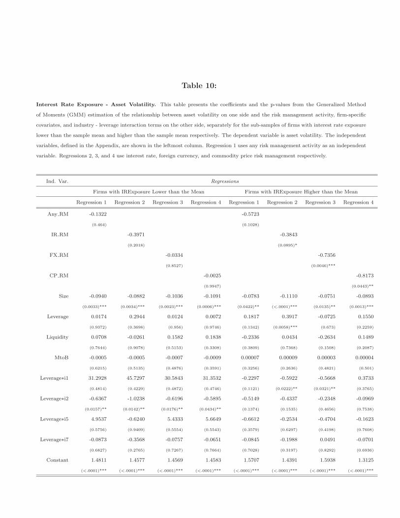
Table 10:

Interest Rate Exposure - Asset Volatility. This table presents the coefficients and the p-values from the Generalized Method

of Moments (GMM) estimation of the relationship between asset volatility on one side and the risk management activity, firm-specific

covariates, and industry - leverage interaction terms on the other side, separately for the sub-samples of firms with interest rate exposure

lower than the sample mean and higher than the sample mean respectively. The dependent variable is asset volatility. The independent

variables, defined in the Appendix, are shown in the leftmost column. Regression 1 uses any risk management activity as an independent

variable. Regressions 2, 3, and 4 use interest rate, foreign currency, and commodity price risk management respectively.

Ind. Var. Regressions

Firms with IRExposure Lower than the Mean Firms with IRExposure Higher than the Mean

Regression 1 Regression 2 Regression 3 Regression 4 Regression 1 Regression 2 Regression 3 Regression 4

Any RM -0.1322 -0.5723

(0.464) (0.1028)

IR RM -0.3971 -0.3843

(0.2018) (0.0895)*

FX RM -0.0334 -0.7356

(0.8527) (0.0046)***

CP RM -0.0025 -0.8173

(0.9947) (0.0443)**

Size -0.0940 -0.0882 -0.1036 -0.1091 -0.0783 -0.1110 -0.0751 -0.0893

(0.0033)*** (0.0034)*** (0.0023)*** (0.0006)*** (0.0422)** (<.0001)*** (0.0135)** (0.0013)***

Leverage 0.0174 0.2944 0.0124 0.0072 0.1817 0.3917 -0.0725 0.1550

(0.9372) (0.3698) (0.956) (0.9746) (0.1342) (0.0058)*** (0.673) (0.2259)

Liquidity 0.0708 -0.0261 0.1582 0.1838 -0.2336 0.0434 -0.2634 0.1489

(0.7644) (0.9078) (0.5153) (0.3308) (0.3809) (0.7368) (0.1508) (0.2087)

MtoB -0.0005 -0.0005 -0.0007 -0.0009 0.00007 0.00009 0.00003 0.00004

(0.6215) (0.5135) (0.4876) (0.3591) (0.3256) (0.2636) (0.4821) (0.501)

Leverage∗i1 31.2928 45.7297 30.5843 31.3532 -0.2297 -0.5922 -0.5668 0.3733

(0.4814) (0.4229) (0.4872) (0.4746) (0.1121) (0.0222)** (0.0321)** (0.3765)

Leverage∗i2 -0.6367 -1.0238 -0.6196 -0.5895 -0.5149 -0.4337 -0.2348 -0.0969

(0.0157)** (0.0142)** (0.0176)** (0.0434)** (0.1374) (0.1535) (0.4656) (0.7538)

Leverage∗i5 4.9537 -0.6240 5.4333 5.6649 -0.6612 -0.2534 -0.4704 -0.1623

(0.5756) (0.9409) (0.5554) (0.5543) (0.3579) (0.6297) (0.4198) (0.7608)

Leverage∗i7 -0.0873 -0.3568 -0.0757 -0.0651 -0.0845 -0.1988 0.0491 -0.0701

(0.6827) (0.2765) (0.7267) (0.7664) (0.7028) (0.3197) (0.8292) (0.6936)

Constant 1.4811 1.4577 1.4569 1.4583 1.5707 1.4391 1.5938 1.3125

(<.0001)*** (<.0001)*** (<.0001)*** (<.0001)*** (<.0001)*** (<.0001)*** (<.0001)*** (<.0001)***

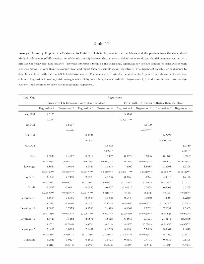
Table 11:

Foreign Currency Exposure - Distance to Default. This table presents the coefficients and the p-values from the Generalized

Method of Moments (GMM) estimation of the relationship between the distance to default on one side and the risk management activity,

firm-specific covariates, and industry - leverage interaction terms on the other side, separately for the sub-samples of firms with foreign

currency exposure lower than the sample mean and higher than the sample mean respectively. The dependent variable is the distance to

default calculated with the Black-Scholes-Merton model. The independent variables, defined in the Appendix, are shown in the leftmost

column. Regression 1 uses any risk management activity as an independent variable. Regressions 2, 3, and 4 use interest rate, foreign

currency, and commodity price risk management respectively.

Ind. Var. Regressions

Firms with FX Exposure Lower than the Mean Firms with FX Exposure Higher than the Mean

Regression 1 Regression 2 Regression 3 Regression 4 Regression 1 Regression 2 Regression 3 Regression 4

Any RM 0.5175 5.3782

(0.646) (0.0024)***

IR RM 0.8597 3.5109

(0.436) (0.0239)**

FX RM 0.1831 5.7272

(0.8301) (0.0086)***

CP RM -4.6942 4.4880

(0.0856)* (0.0894)*

Size 0.5032 0.4867 0.5514 0.7937 0.0972 0.5065 0.1166 0.4932

(0.0422)** (0.0344)** (0.015)** (0.0026)*** (0.7079) (0.0002)*** (0.6902) (0.0071)***

Leverage -3.8944 -4.0759 -3.9445 -4.0845 -7.3700 -8.8085 -4.3698 -4.0398

(0.0016)*** (0.0009)*** (0.0017)*** (0.0035)*** (<.0001)*** (<.0001)*** (0.032)** (0.0012)***

Liquidity 2.6569 2.7488 2.5380 2.7896 3.2658 0.6224 4.0815 1.2175

(0.0178)** (0.0098)*** (0.0224)** (0.0286)** (0.0283)** (0.4407) (0.028)** (0.093)*

MtoB -0.0067 -0.0061 -0.0065 -0.007 -0.01915 0.0058 0.0063 0.0255

(0.0039)*** (0.0014)*** (0.0047)*** (0.0211)** (0.5834) (0.812) (0.8594) (0.0477)**

Leverage∗i1 2.4804 2.6865 2.3808 3.9298 2.5843 5.3042 4.9609 -1.7340

(0.1779) (0.1469) (0.2107) (0.1531) (0.0897)* (0.0043)*** (0.0367)** (0.5502)

Leverage∗i2 3.6925 3.7973 3.4766 3.4813 8.0209 8.7762 7.2632 4.5905

(0.0114)** (0.0074)*** (0.0096)*** (0.0121)** (0.0383)** (0.0003)*** (0.0529)* (0.0275)**

Leverage∗i5 3.8440 3.5182 3.0871 0.8118 -6.3857 7.3571 21.8174 23.6858

(0.2891) (0.3383) (0.3264) (0.812) (0.4055) (0.6232) (0.0985)* (0.006)***

Leverage∗i7 2.8481 3.0269 2.8497 2.8233 5.8053 5.7883 3.0364 1.3849

(0.0258)** (0.0166)** (0.0275)** (0.0586)* (0.0002)*** (0.0013)*** (0.1145) (0.2511)

Constant -0.2021 -0.0227 -0.1614 -0.9773 0.0189 0.4794 -0.9315 -0.1898

(0.8412) (0.9818) (0.8708) (0.4069) (0.9856) (0.516) (0.4257) (0.8304)

Table 12:

Foreign Currency Exposure - Asset Volatility. This table presents the coefficients and the p-values from the Generalized Method

of Moments (GMM) estimation of the relationship between asset volatility on one side and the risk management activity, firm-specific

covariates, and industry - leverage interaction terms on the other side, separately for the sub-samples of firms with foreign currency

exposure lower than the sample mean and higher than the sample mean respectively. The dependent variable is asset volatility. The

independent variables, defined in the Appendix, are shown in the leftmost column. Regression 1 uses any risk management activity as

an independent variable. Regressions 2, 3, and 4 use interest rate, foreign currency, and commodity price risk management respectively.

Ind. Var. Regressions

Firms with FXExposure Lower than the Mean Firms with FXExposure Higher than the Mean

Regression 1 Regression 2 Regression 3 Regression 4 Regression 1 Regression 2 Regression 3 Regression 4

Any RM -0.5903 -0.1611

(0.017**) (0.5984)

IR RM -0.5583 -0.6867

(0.0294**) (0.0071)***

FX RM -0.5422 -1.0470

(0.0659)* (0.0536)*

CP RM 0.2441 -0.9129

(0.5233) (0.0881)*

Size -0.0537 -0.0671 -0.0724 -0.1182 -0.1246 -0.1159 -0.0355 -0.1106

(0.0889)* (0.0163)** (0.008)*** (<.0001)*** (0.0017)*** (<.0001)*** (0.5629) (0.0003)***)

Leverage 0.0513 0.3361 -0.0858 0.1830 0.1910 0.5343 -0.2161 0.0649

(0.712) (0.0261)** (0.6247) (0.1485) (0.1812) (0.0041)*** (0.4957) (0.7005)

Liquidity -0.2536 -0.1090 -0.2151 0.0733 0.3058 0.0965 -0.2067 0.2945

(0.1694) (0.4221) (0.2554) (0.552) (0.2445) (0.6265) (0.5806) (0.0766)*

MtoB 0.00008 0.0001 0.00009 0.0001 -0.0021 0.0006 0.0003 -0.0018

(0.3231) (0.1014) (0.2318) (0.139) (0.4034) (0.8526) (0.9083) (0.4265)

Leverage∗i1 -0.2851 -0.5457 -0.3878 -0.3326 -0.3232 -1.0099 -0.8133 0.5569

(0.284) (0.0576)* (0.1427) (0.3491) (0.0311)** (0.0023)***) (0.0656)* (0.3728)

Leverage∗i2 -0.125 -0.2683 0.0127 -0.1187 -1.0576 -1.5087 -1.0702 -0.9528

(0.6399) (0.3703) (0.968) (0.6812) (0.0001)*** (<.0001)*** (0.0085)*** (<.0001)***

Leverage∗i5 -0.5137 -0.1707 -0.1337 0.2447 -1.2464 -1.9183 -1.8046 -2.0546

(0.3935) (0.7448) (0.8048) (0.6184) (0.1315) (0.0056)*** (0.4447) (0.0221)**

Leverage∗i7 -0.0822 -0.3020 0.0732 -0.1073 -0.3104 -0.5012 -0.2335 -0.1914

(0.578) (0.0678)* (0.6482) (0.4516) (0.2343) (0.0602)* (0.5205) (0.4481)

Constant 1.4885 1.2708 1.4878 1.3654 1.5869 1.6130 1.6362 1.5160

(<.0001)*** (<.0001)*** (<.0001)*** (<.0001)*** (<.0001)*** (<.0001)*** <.0001)*** <.0001)***

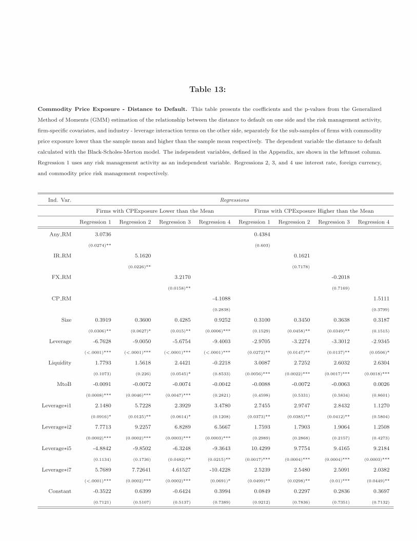
Table 13:

Commodity Price Exposure - Distance to Default. This table presents the coefficients and the p-values from the Generalized

Method of Moments (GMM) estimation of the relationship between the distance to default on one side and the risk management activity,

firm-specific covariates, and industry - leverage interaction terms on the other side, separately for the sub-samples of firms with commodity

price exposure lower than the sample mean and higher than the sample mean respectively. The dependent variable the distance to default

calculated with the Black-Scholes-Merton model. The independent variables, defined in the Appendix, are shown in the leftmost column.

Regression 1 uses any risk management activity as an independent variable. Regressions 2, 3, and 4 use interest rate, foreign currency,

and commodity price risk management respectively.

Ind. Var. Regressions

Firms with CPExposure Lower than the Mean Firms with CPExposure Higher than the Mean

Regression 1 Regression 2 Regression 3 Regression 4 Regression 1 Regression 2 Regression 3 Regression 4

Any RM 3.0736 0.4384

(0.0274)** (0.603)

IR RM 5.1620 0.1621

(0.0226)** (0.7178)

FX RM 3.2170 -0.2018

(0.0158)** (0.7169)

CP RM -4.1088 1.5111

(0.2838) (0.3799)

Size 0.3919 0.3600 0.4285 0.9252 0.3100 0.3450 0.3638 0.3187

(0.0306)** (0.0627)* (0.015)** (0.0006)*** (0.1529) (0.0458)** (0.0349)** (0.1515)

Leverage -6.7628 -9.0050 -5.6754 -9.4003 -2.9705 -3.2274 -3.3012 -2.9345

(<.0001)*** (<.0001)*** (<.0001)*** (<.0001)*** (0.0272)** (0.0147)** (0.0137)** (0.0506)*

Liquidity 1.7793 1.5618 2.4421 -0.2218 3.0087 2.7252 2.6032 2.6304

(0.1073) (0.226) (0.0545)* (0.8533) (0.0056)*** (0.0022)*** (0.0017)*** (0.0018)***

MtoB -0.0091 -0.0072 -0.0074 -0.0042 -0.0088 -0.0072 -0.0063 0.0026

(0.0008)*** (0.0046)*** (0.0047)*** (0.2821) (0.4598) (0.5331) (0.5834) (0.8601)

Leverage∗i1 2.1480 5.7228 2.3929 3.4780 2.7455 2.9747 2.8432 1.1270

(0.0916)* (0.0125)** (0.0614)* (0.1208) (0.0373)** (0.0385)** (0.0412)** (0.5804)

Leverage∗i2 7.7713 9.2257 6.8289 6.5667 1.7593 1.7903 1.9064 1.2508

(0.0002)*** (0.0002)*** (0.0003)*** (0.0003)*** (0.2989) (0.2868) (0.2157) (0.4273)

Leverage∗i5 -4.8842 -9.8502 -6.3248 -9.3643 10.4299 9.7754 9.4165 9.2184

(0.1134) (0.1736) (0.0482)** (0.0215)** (0.0017)*** (0.0004)*** (0.0004)*** (0.0003)***

Leverage∗i7 5.7689 7.72641 4.61527 -10.4228 2.5239 2.5480 2.5091 2.0382

(<.0001)*** (0.0002)*** (0.0002)*** (0.0691)* (0.0499)** (0.0298)** (0.01)*** (0.0449)**

Constant -0.3522 0.6399 -0.6424 0.3994 0.0849 0.2297 0.2836 0.3697

(0.7121) (0.5107) (0.5137) (0.7389) (0.9212) (0.7836) (0.7351) (0.7132)

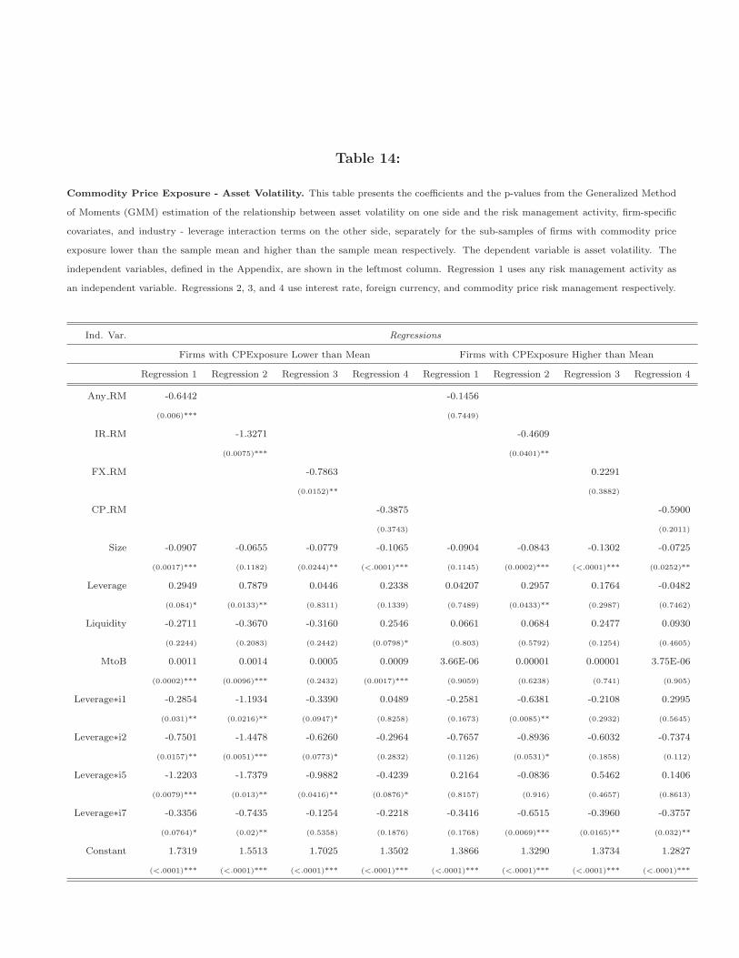
Table 14:

Commodity Price Exposure - Asset Volatility. This table presents the coefficients and the p-values from the Generalized Method

of Moments (GMM) estimation of the relationship between asset volatility on one side and the risk management activity, firm-specific

covariates, and industry - leverage interaction terms on the other side, separately for the sub-samples of firms with commodity price

exposure lower than the sample mean and higher than the sample mean respectively. The dependent variable is asset volatility. The

independent variables, defined in the Appendix, are shown in the leftmost column. Regression 1 uses any risk management activity as

an independent variable. Regressions 2, 3, and 4 use interest rate, foreign currency, and commodity price risk management respectively.

Ind. Var. Regressions

Firms with CPExposure Lower than Mean Firms with CPExposure Higher than Mean

Regression 1 Regression 2 Regression 3 Regression 4 Regression 1 Regression 2 Regression 3 Regression 4

Any RM -0.6442 -0.1456

(0.006)*** (0.7449)

IR RM -1.3271 -0.4609

(0.0075)*** (0.0401)**

FX RM -0.7863 0.2291

(0.0152)** (0.3882)

CP RM -0.3875 -0.5900

(0.3743) (0.2011)

Size -0.0907 -0.0655 -0.0779 -0.1065 -0.0904 -0.0843 -0.1302 -0.0725

(0.0017)*** (0.1182) (0.0244)** (<.0001)*** (0.1145) (0.0002)*** (<.0001)*** (0.0252)**

Leverage 0.2949 0.7879 0.0446 0.2338 0.04207 0.2957 0.1764 -0.0482

(0.084)* (0.0133)** (0.8311) (0.1339) (0.7489) (0.0433)** (0.2987) (0.7462)

Liquidity -0.2711 -0.3670 -0.3160 0.2546 0.0661 0.0684 0.2477 0.0930

(0.2244) (0.2083) (0.2442) (0.0798)* (0.803) (0.5792) (0.1254) (0.4605)

MtoB 0.0011 0.0014 0.0005 0.0009 3.66E-06 0.00001 0.00001 3.75E-06

(0.0002)*** (0.0096)*** (0.2432) (0.0017)*** (0.9059) (0.6238) (0.741) (0.905)

Leverage∗i1 -0.2854 -1.1934 -0.3390 0.0489 -0.2581 -0.6381 -0.2108 0.2995

(0.031)** (0.0216)** (0.0947)* (0.8258) (0.1673) (0.0085)** (0.2932) (0.5645)

Leverage∗i2 -0.7501 -1.4478 -0.6260 -0.2964 -0.7657 -0.8936 -0.6032 -0.7374

(0.0157)** (0.0051)*** (0.0773)* (0.2832) (0.1126) (0.0531)* (0.1858) (0.112)

Leverage∗i5 -1.2203 -1.7379 -0.9882 -0.4239 0.2164 -0.0836 0.5462 0.1406

(0.0079)*** (0.013)** (0.0416)** (0.0876)* (0.8157) (0.916) (0.4657) (0.8613)

Leverage∗i7 -0.3356 -0.7435 -0.1254 -0.2218 -0.3416 -0.6515 -0.3960 -0.3757

(0.0764)* (0.02)** (0.5358) (0.1876) (0.1768) (0.0069)*** (0.0165)** (0.032)**

Constant 1.7319 1.5513 1.7025 1.3502 1.3866 1.3290 1.3734 1.2827

(<.0001)*** (<.0001)*** (<.0001)*** (<.0001)*** (<.0001)*** (<.0001)*** (<.0001)*** (<.0001)***

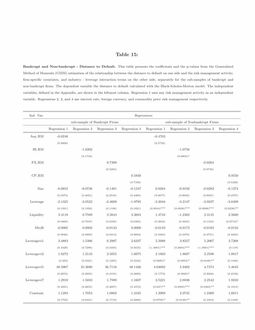
Table 15:

Bankrupt and Non-bankrupt - Distance to Default. This table presents the coefficients and the p-values from the Generalized

Method of Moments (GMM) estimation of the relationship between the distance to default on one side and the risk management activity,

firm-specific covariates, and industry - leverage interaction terms on the other side, separately for the sub-samples of bankrupt and

non-bankrupt firms. The dependent variable the distance to default calculated with the Black-Scholes-Merton model. The independent

variables, defined in the Appendix, are shown in the leftmost column. Regression 1 uses any risk management activity as an independent

variable. Regressions 2, 3, and 4 use interest rate, foreign currency, and commodity price risk management respectively.

Ind. Var. Regressions

sub-sample of Bankrupt Firms sub-sample of Nonbankrupt Firms

Regression 1 Regression 2 Regression 3 Regression 4 Regression 1 Regression 2 Regression 3 Regression 4

Any RM -0.0248 -0.4703

(0.9809) (0.5739)

IR RM -1.0202 -1.0756

(0.1734) (0.0805)*

FX RM 0.7389 -0.0264

(0.5294) (0.9746)

CP RM 0.5830 0.9550

(0.7100) (0.5328)

Size -0.0855 -0.0738 -0.1481 -0.1547 0.0284 -0.0192 -0.0282 -0.1374

(0.5073) (0.4021) (0.2518) (0.4400) (0.8077) (0.8002) (0.8091) (0.4707)

Leverage -2.1325 -2.0522 -2.4609 -1.9795 -3.2044 -3.2147 -2.9237 -2.6499

(0.1501) (0.1356) (0.1196) (0.1821) (0.0044)*** (0.0036)*** (0.0098)*** (0.0238)**

Liquidity 3.4118 0.7589 3.3844 3.3684 1.4743 -1.2362 2.3145 2.5660

(0.0469) (0.7047) (0.0358) (0.0385) (0.3842) (0.4835) (0.1316) (0.0719)*

MtoB -0.0005 0.0002 -0.0143 0.0009 -0.0143 -0.0173 -0.0163 -0.0134

(0.9846) (0.9909) (0.6312) (0.9694) (0.3383) (0.2379) (0.2731) (0.4283)

Leverage∗i1 3.4883 1.5386 6.2987 2.6337 5.5089 3.8257 5.2067 3.7268

(0.4428) (0.7296) (0.3403) (0.5635) (<.0001)*** (0.0004)*** (<.0001)*** (0.119)

Leverage∗i2 1.8272 1.2110 2.5055 1.6075 2.1803 1.8687 2.2598 1.8817

(0.223) (0.3321) (0.1205) (0.2162) (0.0685)* (0.0953)* (0.0448)** (0.1046)

Leverage∗i5 38.3967 35.3690 36.7116 38.1426 4.63092 5.9402 4.7374 5.4845

(0.2853) (0.2695) (0.3155) (0.2889) (0.1773) (0.0829)* (0.2204) (0.2138)

Leverage∗i7 1.2919 1.5033 1.7599 1.1607 2.5221 2.8836 2.2542 1.9233

(0.4001) (0.2855) (0.2897) (0.4372) (0.027)** (0.0095)*** (0.0463)** (0.1013)

Constant 1.1283 1.7053 1.0802 1.4165 1.3989 2.0745 1.2469 1.6811

(0.1702) (0.0441) (0.1719) (0.2066) (0.0705)* (0.0148)** (0.1054) (0.1439)

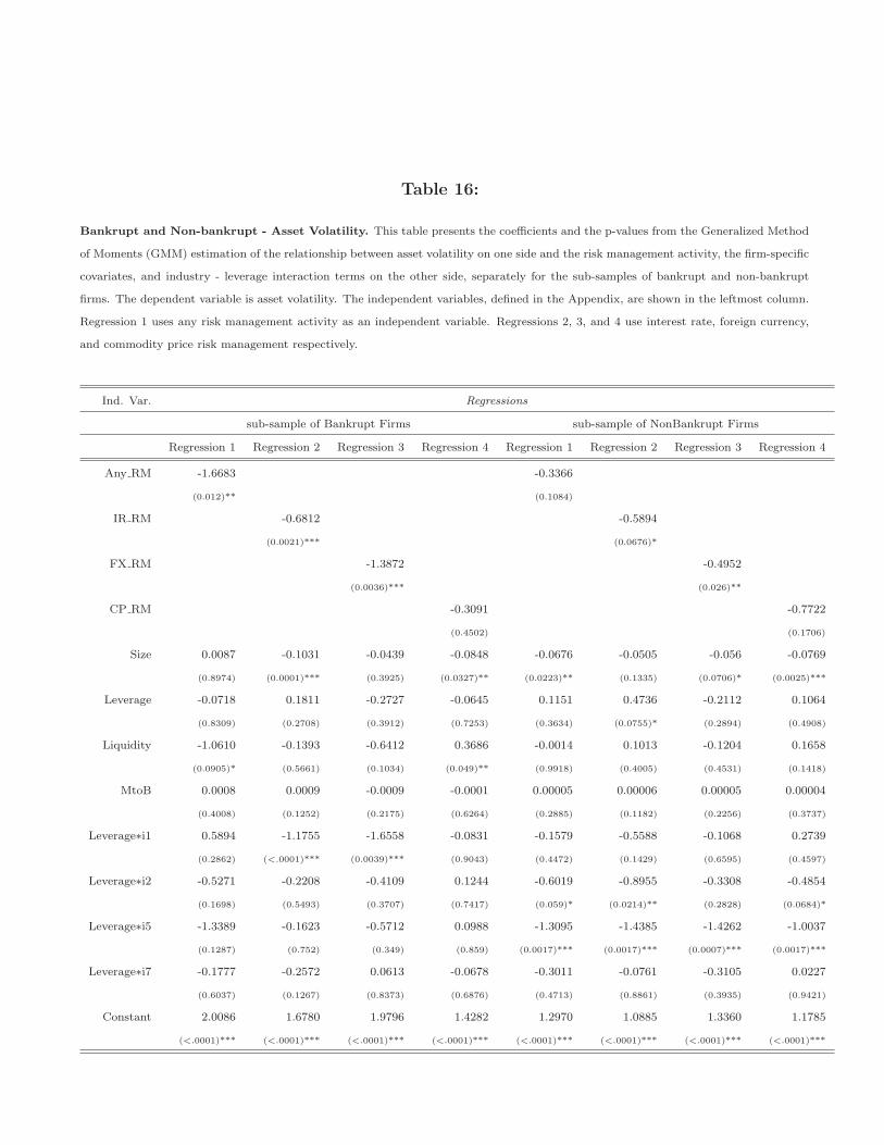
Table 16:

Bankrupt and Non-bankrupt - Asset Volatility. This table presents the coefficients and the p-values from the Generalized Method

of Moments (GMM) estimation of the relationship between asset volatility on one side and the risk management activity, the firm-specific

covariates, and industry - leverage interaction terms on the other side, separately for the sub-samples of bankrupt and non-bankrupt

firms. The dependent variable is asset volatility. The independent variables, defined in the Appendix, are shown in the leftmost column.

Regression 1 uses any risk management activity as an independent variable. Regressions 2, 3, and 4 use interest rate, foreign currency,

and commodity price risk management respectively.

Ind. Var. Regressions

sub-sample of Bankrupt Firms sub-sample of NonBankrupt Firms

Regression 1 Regression 2 Regression 3 Regression 4 Regression 1 Regression 2 Regression 3 Regression 4

Any RM -1.6683 -0.3366

(0.012)** (0.1084)

IR RM -0.6812 -0.5894

(0.0021)*** (0.0676)*

FX RM -1.3872 -0.4952

(0.0036)*** (0.026)**

CP RM -0.3091 -0.7722

(0.4502) (0.1706)

Size 0.0087 -0.1031 -0.0439 -0.0848 -0.0676 -0.0505 -0.056 -0.0769

(0.8974) (0.0001)*** (0.3925) (0.0327)** (0.0223)** (0.1335) (0.0706)* (0.0025)***

Leverage -0.0718 0.1811 -0.2727 -0.0645 0.1151 0.4736 -0.2112 0.1064

(0.8309) (0.2708) (0.3912) (0.7253) (0.3634) (0.0755)* (0.2894) (0.4908)

Liquidity -1.0610 -0.1393 -0.6412 0.3686 -0.0014 0.1013 -0.1204 0.1658

(0.0905)* (0.5661) (0.1034) (0.049)** (0.9918) (0.4005) (0.4531) (0.1418)

MtoB 0.0008 0.0009 -0.0009 -0.0001 0.00005 0.00006 0.00005 0.00004

(0.4008) (0.1252) (0.2175) (0.6264) (0.2885) (0.1182) (0.2256) (0.3737)

Leverage∗i1 0.5894 -1.1755 -1.6558 -0.0831 -0.1579 -0.5588 -0.1068 0.2739

(0.2862) (<.0001)*** (0.0039)*** (0.9043) (0.4472) (0.1429) (0.6595) (0.4597)

Leverage∗i2 -0.5271 -0.2208 -0.4109 0.1244 -0.6019 -0.8955 -0.3308 -0.4854

(0.1698) (0.5493) (0.3707) (0.7417) (0.059)* (0.0214)** (0.2828) (0.0684)*

Leverage∗i5 -1.3389 -0.1623 -0.5712 0.0988 -1.3095 -1.4385 -1.4262 -1.0037

(0.1287) (0.752) (0.349) (0.859) (0.0017)*** (0.0017)*** (0.0007)*** (0.0017)***

Leverage∗i7 -0.1777 -0.2572 0.0613 -0.0678 -0.3011 -0.0761 -0.3105 0.0227

(0.6037) (0.1267) (0.8373) (0.6876) (0.4713) (0.8861) (0.3935) (0.9421)

Constant 2.0086 1.6780 1.9796 1.4282 1.2970 1.0885 1.3360 1.1785

(<.0001)*** (<.0001)*** (<.0001)*** (<.0001)*** (<.0001)*** (<.0001)*** (<.0001)*** (<.0001)***