CAN SHORT SELLING CONSTRAINTS EXPLAIN THE PORTFOLIO

INEFFICIENCY OF U.K. BENCHMARK MODELS?

Jonathan Fletcher

University of Strathclyde

Key words: Mean-Variance Efficiency, Portfolio Constraints, Bayesian Analysis, Factor

Models

JEL classification: G11, G12

The author is from the University of Strathclyde.

Helpful comments received from two anonymous reviewers.

This draft: July 2017

Address correspondence to Professor J. Fletcher, Department of Accounting and Finance,

University of Strathclyde, Stenhouse Building, Cathedral Street, Glasgow, G4 0LN, United

Kingdom, phone: +44 (0) 141 548 4963, fax: +44 (0) 552 3547, email:

j.fletcher@strath.ac.uk

CAN SHORT SELLING CONSTRAINTS EXPLAIN THE PORTFOLIO

INEFFICIENCY OF U.K. BENCHMARK MODELS?

ABSTRACT

This study uses the Bayesian approach of Wang(1998) to examine the impact of no

short selling constraints on the mean-variance inefficiency of linear factor models in U.K.

stock returns and to conduct model comparison tests between the models. No short selling

constraints lead to a substantial reduction in the mean-variance inefficiency of all factor

models and eliminate the mean-variance inefficiency of some factor models in states when

the lagged one-month U.K. Treasury Bill return is higher than normal. In model comparison

tests, the best performing model is a six-factor model of Fama and French(2017a), which uses

the small ends of the value, profitability, investment, and momentum factors.

1

I Introduction

Linear factor models such as the capital asset pricing model (CAPM) and arbitrage

pricing theory (APT) imply the mean-variance efficiency of a given benchmark model

(Roll(1977), Grinblatt and Titman(1987)). A large number of studies document the mean-

variance inefficiency of different benchmark models such as Gibbons, Ross and

Shanken(1989), MacKinlay and Richardson(1991), and Fama and French(2015a,2016)

among others in U.S. stock returns and Fletcher(1994, 2001) and Gregory, Tharyan and

Christidis(2013) among others in U.K. stock returns. These studies usually use the mean-

variance efficiency tests of Gibbons et al.

The Gibbons et al(1989) test of mean-variance efficiency compares the maximum

squared Sharpe(1966) performance of the K factors in the benchmark model to the maximum

squared Sharpe performance of the N test assets and K factors. Fama and French(2015b)

argue that whilst the Gibbons et al test of mean-variance efficiency is a powerful test of asset

pricing models, it is less relevant for practical investment applications as the underlying

optimal portfolios allow for unrestricted short selling. Such portfolios are not attainable for

long-only investors and even where investors can short sell, the costs of short selling can

eliminate much of the performance improvement (Fama and French)1. Tests of mean-

variance efficiency in the presence of short selling constraints exist with Basak, Jagannathan

and Sun(2002) in a classical setting and in a Bayesian framework with Wang(1998).

The issue of no short selling constraints is an important one as many investors do not

engage in short selling, either due to investment restrictions or the costs of short selling are

1 Best and Grauer(1991) highlight the extreme sensitivity of optimal mean-variance portfolio

weights to changes in asset means. They argue that portfolio constraints like no short selling

will almost always be binding as the unconstrained mean-variance frontier can often contain

no all positive weight portfolios (Best and Grauer(1992)).

2

prohibitive. Bris, Goetzmann and Zhu(2007) find that short selling is allowed in 35 out of 47

countries. Even in countries where short selling is allowed, temporary bans can be imposed

such as in the U.K., where short selling in financial stocks was banned in late 2008 until early

2009. Managed open-end funds2 in the U.K. under the EU UCITS regulations are not

allowed to take physical short positions and are only allowed to borrow up to 10%. No short

selling is important as it is known that short selling constraints hurt the mean-variance

performance of trading strategies such as in emerging markets (De Roon, Nijman and

Werker(2001), Li, Sarkar and Wang(2003)) and factor investing (Briere and

Szafarz(2017a,b)).

I use the Bayesian approach of Wang(1998) to examine the impact of no short selling

constraints on tests of mean-variance efficiency of linear factor models in U.K. stock returns.

My study examines three main research questions. First, I examine whether no short selling

constraints can explain the portfolio inefficiency of linear factor models. Second, I examine

the mean-variance efficiency of the linear factor models across economic states. Third, I

conduct model comparison tests between the factor models building on the results in Barillas

and Shanken(2017a). My analysis is important for two reasons. First, if a given benchmark

model lies on the mean-variance frontier in the presence of no short selling constraints, then it

could provide a useful benchmark to evaluate the performance of long-only portfolio

managers3. Second, if a given benchmark model lies on the mean-variance frontier in the

2 Almazan, Brown, Carlson, and Chapman(2004) find that only a tiny fraction of U.S. mutual

funds engage in short selling.

3 Connor and Korajczyk(1991) evaluate U.S. mutual fund performance within an APT

framework.

3

presence of no short selling constraints then it provides a candidate for an optimal portfolio to

hold for investors4.

I test the mean-variance efficiency of eight linear factor models between July 1983

and December 2015 in the presence of no short selling constraints. The models include the

CAPM, Fama and French(1993), Carhart(1997), the five-factor model of Fama and

French(2015a) (FF5), a six-factor model (FF6) of FF5 plus the momentum factor, a five-

factor model (FF5s) which includes the small ends of the value, profitability, and investment

factors (Fama and French(2017a)), a six-factor model (FF6s) which augments FF5s model

with the small end of the momentum factor, and a six-factor model of Asness, Frazzini, Israel

and Moskowitz(2015) (AFIM) which replaces the value factor in the FF6 model with more

timely version (Asness and Frazzini(2013)) of this factor. To test the mean-variance

efficiency of the linear factor models across economic states, I use the dummy variable

approach of Ferson and Qian(2004) to identify three economic states. I use the lagged one-

month U.K. Treasury Bill return as the information variable. The dummy variable approach

identifies each month in the sample as when the lagged Treasury Bill return is lower than

normal (Low), Normal, and higher than normal (High) using only the information prior to

each month.

There are four main findings to my study. First, the lagged one-month Treasury Bill

return has significant predictive ability of the excess returns on the test assets and factors.

Second, no short selling constraints lead to a substantial reduction in the portfolio

inefficiency of each model but the mean-variance efficiency of each model is still rejected.

Third, the tests of mean-variance efficiency vary across economic states. In the High state,

4 This argument ignores the caveat that many benchmark models like Fama and French(1993)

require short positions. In this case, we can consider investors selecting from a set of factors

that are provided by some benchmark provider such as MSCI.

4

there is little evidence against the models. Fourth, in the relative model comparison tests, the

FF6s model has the best overall performance. My study suggests that no short selling

constraints leads to a substantial reduction in portfolio inefficiency and the best performing

model is the FF6s model.

My study makes three contributions to the literature. First, I extend the analysis in

Wang(1998) by looking at multifactor models in addition to the CAPM. My study

complements the recent Fama and French(2015b) study by conducting formal statistical tests

of portfolio efficiency in the presence of no short selling constraints and addressing the mean-

variance efficiency of benchmark models rather the incremental contribution of stock

characteristics. Second, I extend the prior U.K. literature on linear factor models such as

Fletcher(1994, 2001), Clare, Smith and Thomas(1997), Florackis, Gregoriou and

Kostakis(2011), Gregory et al(2013), Davies, Fletcher and Marshall(2014) among others by

focusing on testing portfolio efficiency in the presence of no short selling constraints and

considering the new factor models of Fama and French(2015a, 2017a). Third, my study

complements the Bayesian tests of model comparison in Barillas and Shanken(2017b) by

focusing on the performance of the factor models in U.K. stock returns and comparing

models in the presence of no short selling constraints.

My paper is organized as follows. Section II discusses the research method of my

study. Section III presents the data. Section IV reports the empirical results and the final

section concludes.

II Research Method

The Gibbons et al(1989) test of portfolio efficiency assumes the existence of a risk-

free asset. Define K as the number of factors in the benchmark model, and N as the number

of test assets. Linear factor models such as the CAPM5 and APT imply that either the market

5 See Shih, Chen, Lee and Chen(2014) for a review of alternative CAPM models.

5

portfolio (when K=1) or a portfolio of the K factors lie on the ex ante mean-variance efficient

frontier of the N+K assets. Gibbons et al show that the null hypothesis of mean-variance

efficiency implies that the N intercept terms (alphas) from the multivariate regression of the

N test asset excess returns on a constant and the K factors will be jointly equal to zero.

Gibbons et al assume that the residuals from the multivariate regression are independently

and identically distributed and have a multivariate normal distribution. The test of mean-

variance efficiency is given by:

GRS = [(T-N-K)/N]α’Σ-1α/(1+θ2K) (1)

where α is the (N,1) vector of individual alphas, Σ is the (N,N) Maximum Likelihood (ML)

estimate of the residual covariance matrix, θ2K is the maximum squared Sharpe(1966)

performance of the K factors, and T is the number of observations.

Under the null hypothesis of mean-variance efficiency, the GRS test has a central F

distribution with N and T-N-K degrees of freedom. Gibbons et al(1989) show that the GRS

test can also be written as:

[(T-N-K)/N](θ*2 – θ2K)/(1 + θ2

K) (2)

where θ*2 is the maximum squared sample Sharpe performance of the N+K assets6. Under

the null hypothesis of mean-variance efficiency, θ*2 = θ2K. The Gibbons et al test assumes

that the investor is allowed unrestricted short selling.

Basak et al(2002) develop tests of mean-variance efficiency when investors face no

short selling constraints7. An alternative approach to testing mean-variance efficiency in the

6 Ferson and Siegel(2009) extend the portfolio efficiency tests to the situation where investors

can use conditioning information.

7 De Roon et al(2001) develop the corresponding tests of mean-variance spanning in the

presence of portfolio constraints. See De Roon and Nijman(2001) and Kan and Zhou(2012)

6

presence of no short selling constraints is the Bayesian approach of Wang(1998) and Li et

al(2003)8. Li et al point out that the Bayesian approach has a number of advantages. First,

the uncertainty of finite samples is incorporated into the posterior distribution. Second, the

Bayesian approach is easier to use and can include lots of different portfolio constraints and

performance measures. Third, the asymptotic tests of Basak et al(2002) and De Roon et

al(2001) rely on a first-order linear approximation but the Bayesian test uses the exact

nonlinear function. This approach was developed when no risk-free asset exists but the same

approach can be modified to the case where there is risk-free lending and borrowing.

I measure the portfolio inefficiency of the K-factor benchmark model as:

DSharpe = θ* - θK (3)

where θ* = x’u/(x’Vx)1/2, θK = xb’u/(xb’Vxb)1/2, u is the (N+K,1) vector of expected excess

returns, V is the (N+K,N+K) covariance matrix, x is the (N+K,1) vector of optimal weights

from the mean-variance frontier of the N+K assets, and xb is the (N+K,1) vector of the

optimal weights from the mean-variance frontier of the K assets where the first N cells equal

zero. If the K-factor model is mean-variance efficient, DSharpe = 0. When the risk-free

asset exists, all optimal portfolios (which are combinations of the risk-free asset and the

tangency portfolio) have the same Sharpe performance. As a result, the DSharpe measure

can be estimated using any optimal portfolio on the corresponding mean-variance frontiers of

the K factors and the N+K assets. I estimate the optimal portfolios using a given value of risk

aversion, which I set equal to 3 as in Tu and Zhou(2011). I estimate the DSharpe measure

for a review of traditional tests of mean-variance spanning when there are no constraints

beyond the budget constraint.

8 Recent applications of the Bayesian approach include Hodrick and Zhang(2014) and

Liu(2016) in tests of the benefits of international diversification.

7

using both unconstrained portfolio strategies and constrained portfolio strategies where no

short selling constraints are imposed on the risky assets.

To examine the statistical significance of the DSharpe measure, I use the Bayesian

approach of Wang(1998). The analysis assumes that the N+K asset excess returns have a

multivariate normal distribution9. I assume a non-informative prior for the expected excess

returns u and covariance matrix V. Define us and Vs as the sample moments of the expected

excess returns and covariance matrix, and r as the (T,N+K) matrix of excess returns of the N

assets and K factors. The posterior probability density function is given by:

p(u,V|R) = p(u|V,us,T)p(V|Vs,T) (4)

where p(u|V,us,T) is the conditional distribution of a multivariate normal (us,(1/T)V)

distribution and p(V|Vs,T) is the marginal posterior distribution that has an inverse

Wishart(TV, T-1) distribution (Zellner, 1971)).

Wang(1998) proposes a Monte Carlo method to approximate the posterior

distribution. First, a random V matrix is drawn from an inverse Wishart (TVs,T-1)

distribution. Second, a random u vector is drawn from a multivariate normal (us,(1/T)V)

distribution. Third, given the u and V from steps 1 and 2, the DSharpe measure is estimated

from equation (3)10. Fourth, steps 1 to 3 are repeated 1,000 times as in Hodrick and

Zhang(2014) to generate the approximate posterior distribution of the DSharpe measure. The

posterior distribution of the DSharpe measure is then used to assess the magnitude of the

9 The multivariate normality assumption can be viewed as a working approximation in

monthly returns. Optimal portfolios of mean-variance utility functions are often close to

other utility functions over short horizons (Kroll, Levy and Markowitz(1984), Grauer and

Hakansson(1993), and Best and Grauer(2011)).

10 If the optimal portfolios lie on the inefficient side of the mean-variance frontier, I set the

corresponding Sharpe performance to zero.

8

portfolio inefficiency of the K-factor benchmark and the statistical significance. The average

value from the posterior distribution provides the average increase in the Sharpe performance

in moving from the optimal portfolio of the K factors to the optimal portfolio of the N+K

assets. I use the 5% percentile value of the DSharpe measure to assess the statistical

significance of whether the average DSharpe measure equals zero (Hodrick and Zhang). If

the 5% percentile value of DSharpe measure exceeds zero, I reject the null hypothesis of the

portfolio efficiency of the K-factor benchmark model.

The analysis provides an absolute test for a given factor model. However the mean

DSharpe measures are not strictly comparable across models as the N+K investment universe

differs for each model. A recent study by Barillas and Shanken(2017a) shows that when

comparing factor models using metrics like the Sharpe measure, the N test assets are

irrelevant. For comparing models, the relevant issue is how well the factor models price

factors not included in the model. Define K1 as the number of factors in the union of all the

factors across the eight models. Applying the Barillas and Shanken arguments to the method

used here, if the investment universe is fixed across models as the N test assets and K1

factors, then the optimal portfolio of the N+K1 assets is the same across models. When

comparing the DSharpe measures across models, the θ* term drops out and the relevant

comparison is between the θK implied by each model. As a result, when comparing two

models the DSharpe measure is given by the difference in Sharpe performance between the

two models and the Bayesian approach can be used to estimate the average DSharpe measure

and to evaluate statistical significance.

The analysis so far focuses on testing the portfolio efficiency of each factor model

across the whole sample period. The final issue I examine is to test the portfolio efficiency of

the factor models across different states of the world using the dummy variable approach of

Ferson and Qian(2004) and Ferson, Henry and Kisgen(2006). It might well be the case that

9

the factor models perform better in some states of the world compared to other states. The

dummy variable approach is used as follows. Define zt as the value of the lagged information

variable at time t. A new series xt is constructed by subtracting from zt the mean of zt over

the previous 60 months. We then divide xt by the standard deviation of zt over the prior 60

months σ(zt). Ferson and Qian construct three states11 based on the values of xt/σ(zt). If xt/

σ(zt) < -1, then the month is a Low state. If xt/σ(zt) > 1, the month is a High state. If -1 < xt/

σ(zt) < 1, the month is a Normal state. I use the dummy variable approach to assign each

month in the sample to one of three states. I then run the Bayesian test across the three

subsamples.

The dummy variable approach assigns each month in the sample to a given state using

only information prior to that month and so is known ex ante. This approach contrasts with

using ex post variables such as the NBER recession and expansion states. Ferson and

Qian(2004) also point out that the dummy variables reduces the spurious regression bias of

Ferson, Sarkissian and Simin(2003) when using lagged information variables that are highly

persistent such as the short term interest rate.

III Data

A) Test Assets and Lagged Information Variable

I use two groups of test assets to examine the portfolio efficiency of different linear

factor models in the presence of no short selling constraints between July 1983 and December

2015. The first group is 16 portfolios of stocks sorted by size and book-to-market (BM) ratio.

The second group follows Kirby and Ostdiek(2012) and uses 15 portfolios of stocks sorted by

volatility and momentum. The portfolios are value weighted buy and hold monthly returns.

The portfolios are formed using all U.K. stocks traded on the London Stock Exchange and

11 It is possible to use more than three states, but the number of observations in each state

would decline.

10

smaller investment markets like the Alternative Investment Market. All of the stock return

and market value data is collected from the London Share Price Database (LSPD) provided

by the London Business School. The accounting data is collected from Worldscope provided

by Thompson Financial. I use the one-month U.K. Treasury Bill return as the risk-free asset,

which I collect from LSPD and Datastream. Full details on the construction of the test assets

are provided in the Appendix.

Table 1 reports summary statistics of the monthly excess returns of the two groups of

test assets. The summary statistics include the mean and standard deviation of monthly

excess returns (%) for the size/BM portfolios (panel A) and the volatility/momentum

portfolios (panel B). The size/BM portfolios are ordered by size in the rows from Small to

Big and by the BM ratio in the columns from Low to High. The volatility/momentum

portfolios are sorted by volatility in the rows from Low to High and by momentum in the

columns from Losers to Winners.

Table 1 here

Panel A of Table 1 shows that there is a wide spread in average excess returns across

the size/BM portfolios. The average excess returns range between -0.093% (Small/Growth)

and 0.660% (3/Value). There is a value effect across every size group, where the Value

portfolio has a higher average excess return than the Growth portfolio. The value effect is

stronger in small companies, which is consistent with Fama and French(2012). In contrast,

the size effect varies across the BM groups. For the growth portfolio, large companies have a

higher average excess returns than smaller companies. For the other three BM groups, there

is little size effect.

11

The volatility/momentum portfolios in panel B of Table 1 have a wider spread in both

the mean and volatility of excess returns than the size/BM portfolios. The average excess

returns range between -0.951% (4/Losers) and 0.995% (3/Winners). There is a strong

momentum effect across all five volatility groups. The Winners portfolios have both a higher

mean and lower volatility of excess returns than the Losers portfolios. The momentum effect

is stronger in the high volatility groups. There is a strong volatility effect across the three

past return groups. The volatility effect is stronger in the Losers portfolios, where the low

volatility portfolio has a higher mean and lower volatility of excess returns than the high

volatility portfolio.

I use the dummy variable approach of Ferson and Qian(2004) with the lagged one-

month U.K. Treasury Bill return as the conditioning information. Studies which use a short

interest rate in asset pricing and conditional performance studies include Harvey(1991),

Ferson and Schadt(1996), Ferson and Qian, and Zhang(2006) among others. Table 2 reports

the mean and standard deviation of the excess returns of the size/BM (panel A), and

volatility/momentum (panel B) portfolios across the three economic states. Ferson et

al(2006) point out that we can estimate the standard error for the difference in mean excess

returns in high and low states as 0.05σ(hi)[1+(σ(lo)/σ(hi))2]1/2, where σ(lo) and σ(hi) are the

standard deviation of portfolio excess returns in low and high states.

Table 2 here

Table 2 shows that there is a substantial spread in the mean and volatility of excess

returns of the test assets across the three states for both groups of test assets. The lagged one-

month Treasury Bill return has substantial predictive ability of the mean and volatility of the

test asset excess returns using the dummy variable approach. In the size/BM portfolios, the

12

average excess returns are highest in the Low state and lowest in the High state. The

variation in the mean and volatility across states is much more significant for the smaller firm

portfolios. For the bottom three size groups, the average excess returns in the Low state are

significantly higher than the High state. In the portfolios of big companies, only the Big/3

and Big/Value portfolios that have a significant higher average excess return in the Low state

compared to the High state.

There is a strong size effect across the three states in the size/BM portfolios.

However the direction of the size effect varies. In the Low state, the average excess returns

on the small stock portfolios are considerably higher than the large stock portfolios. In the

Normal and High states, the reverse is true. Large stock portfolios provide higher mean

excess returns than small stock portfolios. In the Normal and High states, the reverse size

effect is stronger in the Growth portfolios.

There is a strong value effect in the Low and Normal states. Value portfolios provide

higher mean excess returns than Growth portfolios. The value effect is stronger in smaller

companies. In the High state, the value effect is weaker and is only strong in the smallest

stock portfolios. It is only in Big stocks, where the Growth portfolio has a higher mean

excess returns than the Value portfolio.

In the volatility/momentum portfolios in panel B of Table 3, in most cases the mean

excess returns are highest in the Low state and lowest in the High state. There is substantial

variation in the mean and volatility of the volatility/momentum portfolios, which is greater

than the size/BM portfolios. For the three largest volatility groups, the mean excess returns

are significantly higher in the Low state compared to the High state. For the bottom two

volatility portfolios, the mean excess returns in the Low state are significantly higher than the

High state for the Low/Losers, 2/Losers, and 2/2 portfolios.

13

The volatility effect varies across the three states. In the Low state, the High volatility

portfolios have a higher mean excess returns than the Low volatility portfolios, but also have

a higher volatility. In the Normal and High states, the mean excess returns and volatility are

considerably lower for the Low volatility portfolios rather than the High volatility portfolios.

The volatility effect is stronger in the Losers portfolios in the Normal and High states.

The momentum effect also varies across the three economic states. The momentum

effect is strongest in the High state and weakest in the Low state. In the Low and Normal

states, the mean excess returns between the Winners and Losers portfolios in the Low

volatility group are narrow. In the Normal and High states, the Winners portfolio of the

lower volatility groups performs the best. The pattern in mean excess returns in Table 2

across the three states using the short term interest rate is similar to the equity portfolios in

U.S. stock returns in Ferson and Qian(2004).

B) Factor Models

I consider eight linear factor models in my study12. Details of the construction of the

factor models are included in the Appendix. The models include:

1. CAPM

This model is a single-factor model that uses the excess returns of the U.K. stock

market index (Market) as the proxy for aggregate wealth.

2. Fama and French(1993) (FF)

The FF model is a three-factor model. The factors are the excess return on the market

index and two zero-cost portfolios that capture the size (SMB) and value/growth (HML)

12 A recent study by Bianchi, Drew and Whittaker(2016) evaluate the predictive performance

of different asset pricing models to estimate the cost of equity capital in Australian stock

returns.

14

effects in stock returns. I use the same size factor across models based on the Fama and

French(2015a) model.

3. Carhart(1997)13

The Carhart model is a four-factor model. The factors are the three factors in the FF

model and a zero-cost portfolio that captures the momentum effect (WML) in stock returns.

4. Fama and French(2015a) (FF5)

This model is a five-factor model, which augments the FF model with two zero-cost

portfolios that capture the profitability (RMW) and investment growth (CMA) effects in

stock returns.

5. Fama and French(2017a) FF6

This model is a six-factor model, which augments the FF5 model with the WML

factor.

6. Fama and French(2017a) (FF5s)

This model is a five-factor model which includes the small ends of the HML, RMW,

and CMA factors defined as HMLS, RMWS, and CMAS.

7. Fama and French(2017a) FF6s

This model is a six-factor model, which augments the FF5s model with the small end

of the WML factor (WMLS).

8. Asness, Fazzini, Moskowitz and Israel(2015)

This model is similar to the FF6 model except the HML factor is replaced with the

more timely version of the HML (HMLT) factor of Asness and Frazzini(2013).

13 Maio and Santa-Clara(2012) find that both the Fama and French(1993) and Carhart(1997)

models are the most consistent with ICAPM restrictions across a wide range of different

multifactor models. In contrast, Barbalau, Robotti and Shanken(2015) find that it is very

difficult to find any models which are inconsistent with the ICAPM restrictions.

15

Table 3 reports summary statistics of the monthly excess factor returns for the factors

in the linear factor models. The table includes the mean and standard deviation of the

monthly excess factor returns (%), and the final column reports the unadjusted t-statistic of

the null hypothesis that the average excess factor return equals zero.

Table 3 here

Table 3 shows that a number of factors have significant average excess returns. The

WML and WMLS factors have the highest mean excess returns at 0.935% and 1.255%,

confirming the strong momentum effect in U.K. stock returns. The HML and HMLS factors

have significant positive average excess returns as do the CMA and CMAS factors. The SMB

factor has a tiny average excess returns. Likewise neither the RMW and RMWS factors have

significant average excess returns, which differ from Fama and French(2015a,2016,2017a)

and Novy-Marx(2013).

The results for the RMW and CMA factors differ from Nichol and Dowling(2014).

They find a significant positive average excess return on the RMW factor and a tiny average

excess return on the CMA factor. The difference stems from the sample period they use and

they form the factors only using the largest 350 stocks (in the FTSE 350 index). The use of

the small ends of the factors only makes a difference for the HML and WML factors. For the

RMW and CMA factors, there is little difference in the average excess returns between the

RMW and RMWS factors, and the CMA and CMAS factors. Likewise using the more timely

versions of the SMB and HML factors yields similar average excess returns.

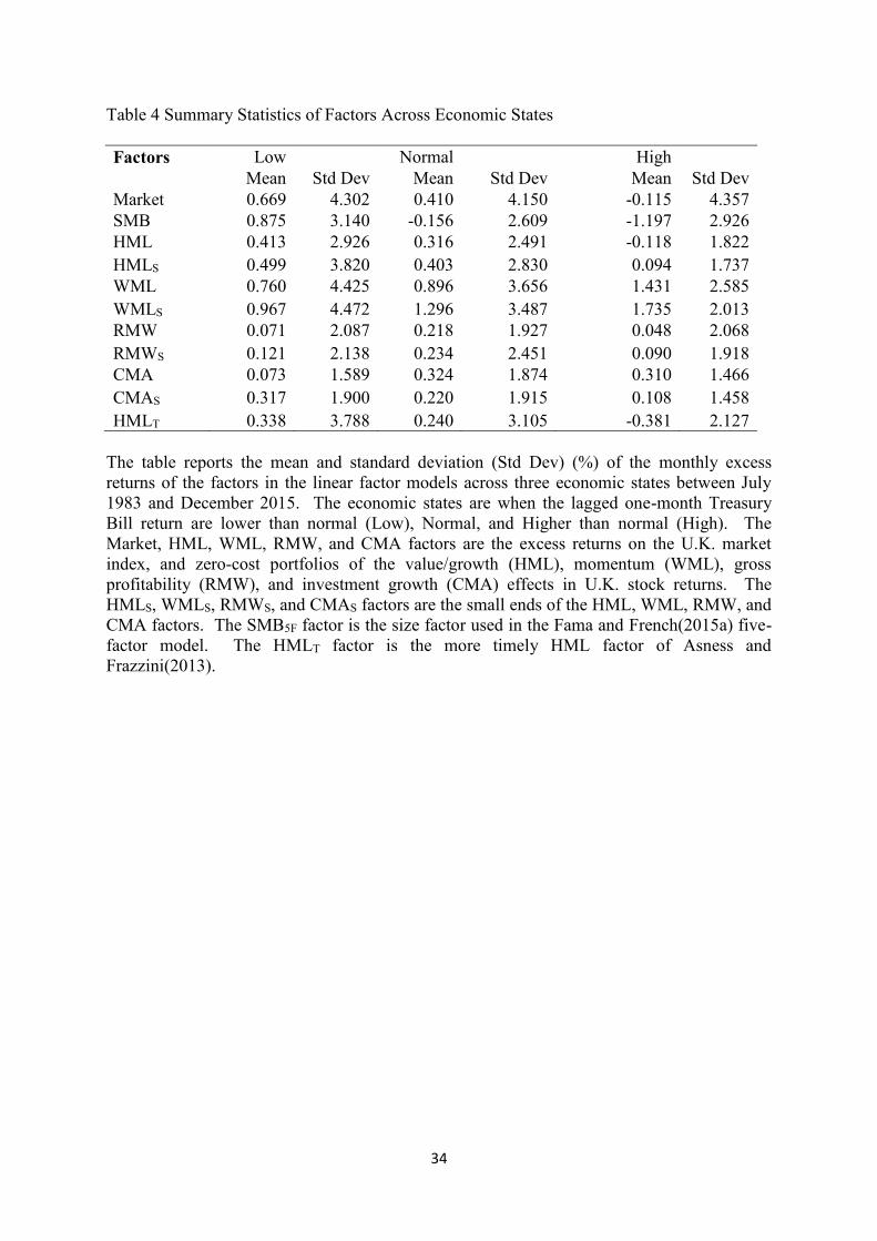
Table 4 reports the mean and volatility of the factors across the three economic states.

Table 4 shows that there is substantial variation in the mean and volatility of the factors

across the three states. The lagged one-month Treasury Bill return has significant predictive

16

ability for most factors using the dummy variable approach of Ferson and Qian(2004). It is

only for the RMW, RMWS, and CMAS factors where the average excess returns in the Low

and High states are not significantly different from one another. For the Market, HML,

HMLS, SMB, and HMLT factors, the mean excess returns are significantly higher in the Low

state compared to the High state. For the WML, WMLS, and CMA factors, the average

excess returns are significantly higher in the High state compared to the Low state. The SMB

factor has the largest variation in mean excess returns across states among the factors. This

result stands in sharp contrast to the tiny mean excess returns of the SMB factor for the whole

sample period. This finding suggests that the dummy variable approach of Ferson and

Qian(2004) picks up interesting variation in the factor excess returns and might have a

significant impact on the performance of the linear factor models in different states.

IV Empirical Results

I begin my empirical analysis by examining the portfolio efficiency of each linear

factor model in unreported tests14. Investors are allowed unrestricted short selling. I examine

the portfolio efficiency of each model over the whole sample period and across the three

economic states. The mean-variance efficiency of each linear factor model is rejected for

both sets of test assets for the whole sample period. All of the mean DSharpe measures are

significant at the 5% percentile. The optimal portfolios behind the increase in Sharpe

performance do require substantial leverage and have large short positions. There is

substantial variation in the magnitude of the mean-variance inefficiency across the three

economic states. All of the models are strongly rejected but the magnitude of the rejection is

substantially higher in the High state. The amount of leverage in the optimal portfolios in the

High state is massive.

14 Results are available on request.

17

The tests of portfolio efficiency allowing for unrestricted short selling show that

investors could increase their Sharpe performance by adding either group of test assets to the

investment universe implied by each factor model. The rejection of mean-variance efficiency

of the factor models is similar to Fletcher(1994, 2001)15 and also the evidence in U.S. stock

returns such as Wang(1998) and Fama and French(2015a,2016a,b) among others. The

pattern in the leverage of the optimal portfolios is consistent with Fama and French(2015b),

who argue that this superior performance is unattainable by long-only investors and even for

investors who can short sell, the superior performance could be greatly reduced due to short

selling costs.

Given that the portfolio efficiency of each factor model is rejected, I next examine the

impact of no short selling constraints on the tests of portfolio efficiency. Table 5 reports the

summary statistics of the posterior distribution of the DSharpe measure using the constrained

portfolio strategies. The summary statistics include the mean, standard deviation, fifth

percentile (5%), and the median of the posterior distribution. Panel A refers to the size/BM

portfolios and panel B to the volatility/momentum portfolios.

Table 5 here

Table 5 shows that the mean-variance efficiency of each linear factor model is

rejected in both sets of test assets in the presence of no short selling constraints. The mean

DSharpe measures range between 0.019 (Carhart) and 0.054 (CAPM) for the size/BM

portfolios and between 0.031 (Carhart) and 0.096 (CAPM) for the size/momentum portfolios.

15 Gregory et al(2013) find that the mean-variance efficiency of U.K. benchmark models

depends upon the portfolio formation method used.

18

The median DSharpe measures are close to the mean DSharpe measures. All of the mean

DSharpe measures are significant at the 5% percentile.

Imposing no short selling constraints on the portfolio efficiency tests has two effects.

First, it leads to a sharp drop in the mean DSharpe measures for each model. No short selling

constraints substantially reduce the magnitude of the portfolio inefficiency of the factor

models but does not eliminate it. This result is consistent with Wang(1998) and Basak et

al(2002). Second, no short selling constraints leads to a drop in the standard deviation of the

posterior distribution of the DSharpe measures. This result is consistent with Wang and Li et

al(2003). Li et al suggest that this result happens because no short selling constraints reduce

the estimation risk in sample mean-variance portfolios (Frost and Savarino(1988) and

Jagannathan and Ma(2003)). This result differs from Basak et al, who found the standard

errors increase of their mean-variance inefficiency measure with no short selling constraints.

Basak et al point out that this is due to the asymptotic test relying on a linear approximation

of a nonlinear function, which is less reliable with no short selling constraints.

The results in Table 5 are consistent with Wang(1998) for the CAPM and extends that

evidence to multifactor models. I next examine the tests of portfolio efficiency of each linear

factor model in the presence of no short selling constraints across the three economic states.

Tables 6 and 7 report summary statistics of the posterior distribution of the DSharpe

measures across the Low (panel A), Normal (panel B), and High (panel C) states. Tables 6

and 7 refer to the size/BM portfolios and volatility/momentum portfolios as the test assets

respectively.

Table 6 here

Table 7 here

19

Table 6 shows that the tests of portfolio efficiency using the constrained portfolio

strategies varies across economic states using the size/BM portfolios as the test assets. Th

most striking result is in panel C where the mean-variance efficiency of each factor model

cannot be rejected. None of the mean DSharpe measures are significant at the 5% percentile.

This result is striking as when unrestricted short selling is allowed, the mean DSharpe

measures are massive and considerably higher than the other states. No short selling

constraints completely eliminates the mean-variance inefficiency of the linear factor models

in the High state.

The linear factor models have their poorest performance in the Low state. The mean

DSharpe measures are the highest in this state and range between 0.082 (FF6s) and 0.293

(CAPM). All of the mean DSharpe measures are significant at the 5% percentile and the

mean-variance efficiency of each factor model is rejected. In the Normal state, the magnitude

of the mean DSharpe measure is only marginally higher than in the High state in most cases.

However, the mean-variance efficiency of each factor model is rejected in the Normal state.

This result occurs because the standard deviation of the DSharpe measures are lower in the

Normal state.

Table 7 shows that the mean-variance efficiency of each linear factor model is

rejected in the Low and Normal states when using the volatility/momentum portfolios as the

test assets. All of the mean DSharpe measures are significant at the 5% percentile. There is

less variation in the mean DSharpe measures across the three states compared to the size/BM

portfolios. For each model, the mean and standard deviation of the DSharpe measures are

lower in the Normal state. In the High state, we are unable to reject the mean-variance

efficiency of the CAPM, FF, Carhart, FF6, and AFIM models and the other models are on the

borderline of statistical significance. However the failure to reject the mean-variance

20

efficiency of some models stems from the higher volatility of the DSharpe measures,

especially for the CAPM and FF models.

Tables 6 and 7 suggest that the performance of the linear factor models varies across

the three economic states. No short selling constraints has the biggest impact in the High

state and eliminates the mean-variance inefficiency of the linear factor models using the

size/BM portfolios and for some models using the volatility/momentum portfolios. This

result is partly due to a higher volatility of the DSharpe measure in the High state compared

to the Normal state. In most cases, the performance of the models is poorest in the Low state.

Tables 5 to 7 suggest that there is evidence of the mean-variance inefficiency of each

factor model in the presence of no short selling constraints. No short selling constraints lead

to a substantial reduction in the mean-variance inefficiency of the linear factor models. This

result is consistent with Wang(1998) and Basak et al(2002). Fama and French(2015b) find

that no short selling constraints eliminates the incremental contribution to the investment

opportunity set of adding a third characteristic to predict expected returns given the other two

characteristics16.

The mean DSharpe measures provide a test of the absolute fit of a model but the

magnitude of the mean DSharpe measures are not comparable across models as the

investment universe of the N+K assets changes with each model. Barillas and

Shanken(2017a,b) show that if the investment universe is fixed across models, then the

choice of test assets becomes irrelevant in the relative model comparison tests. In the

application here θ*2 is fixed and so the relevant comparison is between the maximum Sharpe

performance of each model. I conduct model comparison tests between every pair of factor

models for the whole sample period (panel A) and across the three economic states (panels B

to D). Table 8 reports the mean DSharpe measures between models. Where the mean

16 Fama and French(2015b) focus on the size, BM, and momentum characteristics.

21

DSharpe measure is positive (negative), then the model in the row has a higher (lower)

Sharpe performance than the model in the column. To test for statistical significance, I

examine whether the 5% (95%) percentile is greater (lower) than zero when the mean

DSharpe measure is positive (negative) and denote statistical significance.

Table 8 here

Table 8 shows that the CAPM significantly underperforms all the multifactor models

for the whole sample period and across the three economic states. The mean DSharpe

measures between the CAPM and multifactor models are highly significant. The exception to

this pattern is the insignificant mean DSharpe measure between the CAPM and FF models in

the High state. The relative performance between the CAPM and multifactor models varies

across economic states. For models that include a momentum factor (Carhart, FF6, FF6s, and

AFIM), the mean DSharpe measures are highest in the High state. This result is driven by the

fact that the momentum factors have a much larger average excess return in the High state.

For the FF, FF5, and FF5s models, the mean DSharpe measures are highest in the Low state.

The FF model also performs poorly relative to the alternative multifactor models. The

FF model has a significant lower Sharpe performance relative to the alternative multifactor

models. The mean DSharpe measures are all significant across the whole sample period and

the three economic states. As with the CAPM, the magnitude of the mean DSharpe measures

varies across the economic states. However in contrast to the CAPM, the underperformance

of the FF model is smallest in the Low state. When comparing the FF model to models that

include a momentum factor, the underperformance is largest in the High state. The superior

performance of the FF5 and FF5s models relative to the FF model is consistent with Fama

and French(2015a,2016,2017a) in U.S. stock returns.

22

The Carhart model performs well relative to the two five-factor models. The mean

DSharpe measures between the Carhart model and the FF5 and FF5s models are insignificant

for the whole sample period and the Low and Normal states. The Carhart model significantly

outperforms the FF5 and FF5s models in the High state due to the very strong performance of

the momentum factor. The Carhart model does underperform the three six-factor models.

The mean DSharpe measures between the Carhart model and the FF6s and AFIM models are

significant across the whole sample period and the three economic states. The mean DSharpe

measures between the Carhart and FF6 models are only significant in the Normal and High

state. The FF6s model has the strongest outperformance of the Carhart model in the High

state, which stems from the performance of the WMLS factor in this state. The superior

performance of the six-factor models relative to the Carhart model suggests the importance of

the profitability and investment factors.

The FF5 and FF5s models yield similar performance to one another. None of the

mean DSharpe measures are significant across the whole sample period and the three

economic states. This result is consistent with Fama and French(2017a). The two five-factor

models underperform the six-factor models. Across the whole sample period the mean

DSharpe measures are significant. The FF5 model significantly underperforms the FF6,

FF6s, and AFIM models across the three economic states. The FF5s model yields significant

underperformance relative to the FF6s model across the three states and the FF6 and AFIM

models in the Normal and High states. The magnitude of the underperformance is largest in

the High state, again due to the strong performance of the WML and WMLS factors.

Among the three six-factor models, the FF6 model significantly underperforms the

FF6s and AFIM models across the whole sample period. The FF6 and AFIM models yield

similar Sharpe performance across the three economic states. This result suggests that using

a more timely version of the HML factor (Asness and Frazzin(2013)) has only a limited

23

impact. The FF6s model significantly outperforms the FF6 model across all three economic

states. The FF6s model only significantly outperforms the AFIM model in the High state.

The mean DSharpe measures between the FF6s model and the FF6 and AFIM models are

large in the High state due to the performance of the WMLS factor.

Table 8 suggests that the two best performing models are the FF6s and AFIM models

in the model comparison tests. The FF6s model is the winning model between the two

models due to the large outperformance in the High state. The relative model performance

does depend upon the economic state, with the most pronounced differences in Sharpe

performance taking place in the High state due to the strong performance of the momentum

factors in this state. The interesting part in this result is the fact that in the High state where

there is little evidence against the mean-variance efficiency of the factor models in the

presence of no short selling constraints. This result suggests that even where models are not

rejected, that there can be substantive differences in relative model performance.

V Conclusions

This paper examines the impact of no short selling constraints has on the tests of

mean-variance efficiency of linear factor models and model comparison tests in U.K. stock

returns. There are four main findings from my study. First, using the dummy variable

approach of Ferson and Qian(2004), the lagged one-month Treasury Bill return has

significant predictive ability of the excess returns of the test assets and factors. The test

assets and some of the factors (Market, SMB, HML, HMLS, CMAS, and HMLT) have their

highest average excess returns in the Low state. The momentum factors have their highest

average excess returns in the High state. There is a huge spread in average excess returns

across the three states. The most striking result is for the SMB factor. The SMB factor has a

tiny average excess return across the whole sample period but has the widest spread in mean

excess returns across the three economic states among all the factors. The predictive ability

24

of the lagged one-month Treasury Bill return is consistent with Ferson and Qian(2004) and

Ferson et al(2006).

Second, imposing no short selling constraints leads to a substantial reduction in the

mean-variance inefficiency of the linear factor models. However the mean-variance

efficiency of each factor model is still rejected in both sets of test assets. No short selling

constraints reduce the mean-variance inefficiency of the factor models because the optimal

portfolios in the unconstrained mean-variance efficiency tests require substantial leverage and

large short positions. Fama and French(2015b) argue that such portfolios are not attainable

for long-only investors and the magnitude of short selling costs could eliminate much of the

superior performance of the optimal unconstrained portfolios. This finding is similar to

Wang(1998) and generalizes the evidence to multifactor models.

Third, the mean-variance inefficiency of the linear factor models in the presence of no

short selling constraints varies across the three economic states. The models perform well in

the High state and there is little evidence against the mean-variance efficiency of the linear

factor models. The models are rejected in the Low and Normal states. The reason for the

performance of the models in the High state is the optimal unconstrained portfolios are a lot

more extreme in the High state and so imposing no short selling constraints has a much

bigger impact on the mean-variance efficiency tests in this state.

Fourth, in the model comparison tests, the two best performing models are the FF6s

and AFIM models across the whole sample period. It is important to include either the small

ends of the value, profitability, investment, and momentum factors or include a more timely

version of the HML factor as in Asness and Frazzini(2013) and Asness et al(2015). The

magnitude of the model comparison tests varies across economic states. The difference in

Sharpe performance between the models is largest in the High state due to the performance of

the momentum factors in this state. This result is interesting as there is little evidence of

25

mean-variance inefficiency of the linear factor models in the High state. The FF6s model has

a significant higher Sharpe performance than the AFIM model in the High state and so the

FF6s model is the best performing model in the model comparison tests.

My study suggests that no short selling constraints has a significant impact on the

mean-variance inefficiency of linear factor models in U.K. stock returns and this impact

varies across economic states. The FF6s model has the best performance across the linear

factor models considered followed by the AFIM model. The practical implication of this

research would be to suggest that the FF6s model provides a pretty good benchmark to

evaluate the performance of U.K. equity long-only managed funds. I have focused on

domestic factor models but it would be interesting to make a similar comparison in global

factor models extending the analysis in Fama and French(2012,2017b) and Hou, Karolyi and

Kho(2011). My study has only focused on short selling constraints. The analysis could also

be extended to look at the impact of transaction costs such as in De Roon et al(2001).

Alternatively an examination of more relaxed short selling constraints such as in Briere and

Szafarz(2017b) could be considered. I leave these issues to future research.

26

Appendix

A) Formation of Test Assets

My first set of test assets are 16 size/BM portfolios. I form the portfolios using a

similar approach to Fama and French(2012). At the start of July each year between 1983 and

2015, all stocks on LSPD are ranked independently by their market value at the end of June

and their BM ratio from the prior calendar year. The BM ratio is calculated using the book

value of equity at the fiscal year-end (WC03501) during the previous calendar year from

Worldscope and the year-end market value. I group stocks into four size groups based on

breakpoints of 1%, 3%, and 10% of aggregate market capitalization. I form four BM groups

based on quartile breakpoints of the BM ratios of Big stocks (largest 90% by market value). I

then form 16 size/BM portfolios as the intersection of the independent size and BM groups. I

then calculate value weighted buy and hold monthly returns during the next year, where the

initial weights are the market value weights at the end of June.

I make a number of corrections and exclusions to the portfolio returns which I follow

across forming the test assets and factors. Where a security has missing return observations, I

assign a zero return to the missing values as in Liu and Strong(2008). I correct for the

delisting bias of Shumway(1997) by following the approach of Dimson, Nagel and

Quigley(2003). A –100% return is assigned to the death event date on LSPD where the

LSPD code indicates that the death is valueless. I exclude closed-end funds, foreign

companies, and secondary shares using data from the LSPD archive file. In addition for the

size/BM portfolios, I exclude companies with a zero market value and negative book values.

My second set of test assets stems from Kirby and Ostdiek(2012) and uses 15

volatility/momentum portfolios. At the start of each month between July 1983 and December

2015, I rank all stocks on LSPD by their average absolute returns during the past t-12 to t-2

months and allocate to five volatility groups. Within each volatility group, I then rank all

27

stocks on their past cumulative monthly returns between t-12 to t-2 and group into three

momentum groups. All portfolios have an equal number of stocks as an approximation. I

then estimate the value weighted monthly returns during the next month for the 15

volatility/momentum portfolios using the previous month end market value. I exclude

companies with less than 12 past return observations during the prior year and zero market

values.

B) Formation of Factors in the Linear Factor Models

(i) CAPM

To construct the market index, I use a similar approach to Dimson and Marsh(2001).

At the start of each year between 1983 and 2015, I construct a value weighted portfolio of all

stocks on LSPD. I then calculate the value weighted buy and hold monthly portfolio returns

during the next year, where the initial weights are the market value weights at the end of the

previous year.

(ii) FF

The market index is the same as for the CAPM. To form the HML factor, I use a

similar approach to Fama and French(2012). At the start of July each year between 1983 and

2015, all stocks on LSPD are ranked separately by their market value at the end of June and

by their BM ratio from the prior calendar year. Two size groups (Small and Big) are formed

using a breakpoint of 90% by aggregate market capitalization where the Small stocks are the

companies with smallest 10% by market value and the Big stocks are the companies with the

largest 90% by market value. Three BM groups (Growth, Neutral, and Value) are formed

using break points of the 30th and 70th percentiles of the BM ratios of Big stocks. Six

portfolios of securities are then constructed at the intersection of the size and BM groups (SG,

SN, SV, BG, BN, BV). The monthly buy and hold return for the six portfolios are then

calculated during the next 12 months. The initial weights are set equal to the market value

28

weights at the end of June. Companies with a zero market value, and negative book values

are excluded.

The SMBHML factor is the difference in the average return of the three small firm

portfolios (SG, SN, SV) and the average return of the three large firm portfolios (BG, BN,

BV). The HML factor is the average of HMLS and HMLB where HMLS is the difference in

portfolio returns of SV and SG and HMLB is the difference in portfolio returns of BV and

BG. The HMLS and HMLB zero-cost portfolios capture the value effect in Small stocks and

Big stocks respectively.

(iii) Carhart

The first three factors are the same as the FF model. I form the WML factor using a

similar approach to Fama and French(2012). At the start of each month between July 1983

and December 2015, all stocks on LSPD are ranked separately by their market value at the

end of the previous month and on the basis of their cumulative return from months –12 to –2.

Two size groups (Small and Big) are formed as in the case of the size/BM portfolios. Three

past return groups (Losers, Neutral, and Winners) are formed using break points of the 30th

and 60th percentiles of the past returns of Big stocks. Six portfolios of securities are then

constructed at the intersection of the size and momentum groups (SL, SN, SW, BL, BN,

BW). The value weighted return for the six portfolios are then calculated during the next

month. Companies with a zero market value, and less than 12 return observations during the

past year are excluded from the portfolios.

The WML factor is the average of WMLS and WMLB where WMLS is the difference

in portfolio returns of SW and SL and WMLB is the difference in portfolio returns of BW and

BL. The WMLS and WMLB zero-cost portfolios capture the momentum effect in Small

stocks and Big stocks respectively.

(iv) FF5

29

The market index and HML factor is the same as for the FF model. To form the

SMB, RMW, and CMA factors, I use a similar approach to Fama and French(2015a). At the

start of July each year between 1983 and 2015, I sort stocks separately by market value at the

end of June and either by Gross Profitability (GP) or Investment Growth (Inv) from the prior

calendar year. GP is defined as annual revenues (WC01001) minus cost of goods sold

(WC01051) divided by total assets (WC02999). Inv is defined as the annual change in total

assets divided by total assets. Two size groups are formed as in the case of the size/BM

portfolios. Three GP groups (Weak, Neutral, and Robust) are formed using break points of

the 30th and 70th percentiles of the GP ratios of Big stocks and three Inv groups

(Conservative, Neutral, and Aggressive) are formed using breakpoints of the 30th and 70th

percentiles of the Inv ratios of Big stocks. Six portfolios are then formed of the intersection

between the six size and GP groups (SW, SN, SR, BW, BN, BR) and the six size and Inv

groups(SC, SN, SA, BC, BN, BA). The monthly buy and hold return for the two groups of

six portfolios are then calculated during the next 12 months. The initial weights are set equal

to the market value weights at the end of June. Companies with a zero market value, and

zero or negative sales or cost of goods sold are excluded from the size/GP portfolios.

Companies with zero total assets are excluded from both the size/GP portfolios and the

size/Inv portfolios.

The RMW factor is formed as the average of [(SR-SW)+(BR-BW)] and the CMA

factor is formed as the average of [(SC-SA)+(BC-BA)]. I form a separate size factor from

each of the six size/GP portfolios and size/Inv portfolios. The SMBGP factor is the difference

in the average return of the three small firm portfolios (SW, SN, SR) and the average return

of the three large firm portfolios (BW, BN, BR). The SMBInv factor is the difference in the

average return of the three small firm portfolios (SC, SN, SA) and the average return of the

three large firm portfolios (BC, BN, BA). The SMB factor is given by the average of the

30

SMBHML, SMBGP, and SMBInv factors. Fama and French(2015a) examine alternative

approaches to forming the factors and find that the performance of their five-factor model is

robust as to how the factors are formed.

(v) FF6

This model is the FF5 model and the WML factor

(vi) FF5s

The first two factors are the market and the SMB factors. The HML, RMW, and

CMA factors are formed using the small ends of the factors. The HML factor is given by

HMLS. The RMWS factor is given by the difference in returns between the SR and SW

portfolios. The CMAS factor is given by the difference in returns between the SC and SA

portfolios.

(vii) FF6s

This model is the FF5s model and the small end of the momentum factor given by

WMLS.

(viii) AFIM

This model is motivated by Asness et al(2015). The model is the same as the FF6

model except a more timely version of the HML factor (HMLT) is used. (Asness and

Frazzini(2013)). To form the HMLT factor, I use the following approach. For each month

between July of year t and June of year t+1, all stocks are ranked on the basis of their size and

BM ratio. Size is now measured as the market value at the end of the prior month and BM

ratio is given by the book value from the prior calendar year t-1 divided by the market value

at the end of the prior month. The six size/BM portfolios are then formed as before and the

HMLT factor is formed in the same way as the FF model.

31

Table 1 Summary Statistics of Test Assets

Panel A:

Size/BM

Mean Growth 2 3 Value

Small -0.093 0.320 0.466 0.616

2 -0.042 0.447 0.584 0.536

3 0.256 0.421 0.525 0.660

Large 0.327 0.429 0.476 0.529

σ Growth 2 3 Value

Small 6.372 5.528 5.795 4.703

2 5.843 5.222 5.045 4.909

3 5.599 5.215 5.282 5.340

Large 4.392 4.692 4.885 5.121

Panel B:

Volatility/Momentum

Mean Losers 2 Winners

Low 0.216 0.634 0.687

2 -0.034 0.573 0.857

3 -0.227 0.365 0.955

4 -0.951 0.359 0.843

High -0.638 -0.547 0.582

σ Losers 2 Winners

Low 5.021 4.542 4.279

2 6.446 5.233 4.928

3 8.514 6.276 5.967

4 9.184 7.536 6.939

High 11.328 10.065 8.873

The table reports summary statistics of the monthly excess returns of 16 size/book-to-market

(Size/BM) portfolios (panel A), and 15 volatility/momentum portfolios (panel B), between

July 1983 and December 2015. The summary statistics include the mean and standard

deviation (σ) of monthly excess returns (%). The size/BM portfolios are sorted by size

(Small to Big) and by BM ratio (Low to High). The volatility/momentum portfolios are

sorted by volatility (Low to High) and momentum (Losers to Winners).

32

Table 2 Summary Statistics of Test Assets Across Different Economic States

Panel A:

Size/BM Low

Normal

High

Mean Std Dev Mean Std Dev Mean Std Dev

Small/Growth 1.547 7.420 -0.587 5.926 -1.993 4.301

1.745 6.112 -0.077 5.233 -1.425 4.396

2.331 6.584 -0.114 5.326 -1.629 4.199

Small/Value 2.151 4.760 0.205 4.615 -1.323 3.862

2/Growth 1.144 6.354 -0.389 5.605 -1.449 5.027

1.542 5.484 0.230 5.028 -1.174 4.813

1.791 5.278 0.329 4.955 -1.157 4.197

2/Value 1.869 5.057 0.251 4.769 -1.373 4.276

3/Growth 1.191 6.039 0.078 5.412 -1.152 4.912

1.438 5.398 0.213 5.053 -1.063 4.971

1.303 5.409 0.563 5.089 -1.235 5.285

3/Value 1.655 5.596 0.518 5.203 -0.989 4.815

Big/Growth 0.403 4.082 0.418 4.388 -0.119 5.040

0.490 4.935 0.483 4.595 0.127 4.531

0.869 5.134 0.350 4.744 0.041 4.808

Big/Value 0.704 5.610 0.674 4.759 -0.298 5.157

Panel B:

Volatility/Momentum Low Normal High

Mean Std Dev Mean Std Dev Mean Std Dev

Low/Losers 0.509 5.132 0.462 4.871 -1.186 5.102

0.647 4.499 0.761 4.488 0.206 4.847

Low/Winners 0.797 4.211 0.664 4.315 0.529 4.367

2/Losers 0.332 6.600 0.031 6.578 -1.018 5.641

0.865 5.573 0.594 5.128 -0.107 4.829

2/Winners 1.082 4.749 0.832 5.105 0.463 4.775

3/Losers 1.451 9.870 -0.840 7.915 -1.828 6.592

0.885 6.784 0.217 5.994 -0.259 6.050

3/Winners 1.634 5.864 0.555 6.213 0.794 5.312

4/Losers 0.963 10.540 -1.776 8.249 -2.375 8.391

1.831 8.498 -0.210 7.187 -0.941 5.903

4/Winners 1.951 7.398 0.514 6.804 -0.453 6.084

High/Losers 1.933 14.018 -1.591 9.756 -3.043 8.411

1.837 12.179 -1.542 9.159 -2.423 6.434

High/Winners 2.035 10.024 0.014 8.536 -0.682 6.826

The table reports the mean and standard deviation (Std Dev) (%) of monthly excess returns

for 16 size/BM portfolios (panel A) and 15 volatility/momentum portfolios (panel B) across

three economic states between July 1983 and December 2015. The economic states are when

the lagged one-month Treasury Bill return are lower than normal (Low), Normal, and Higher

than normal (High). The size/BM portfolios are sorted by size (Small to Big) and by BM ratio

(Low to High). The volatility/momentum portfolios are sorted by volatility (Low to High)

and momentum (Losers to Winners).

33

Table 3 Summary Statistics of Factors

Factors Mean σ t-statistic

Market 0.414 4.232 1.932

SMB 0.024 2.927 0.16

HML 0.280 2.557 2.161

HMLS 0.386 3.066 2.481

WML 0.935 3.792 4.871

WMLS 1.255 3.676 6.741

RMW 0.142 2.001 1.40

RMWS 0.173 2.266 1.51

CMA 0.237 1.721 2.721

CMAS 0.235 1.842 2.521

HMLT 0.174 3.229 1.06

1 Significant at 5% 2 Significant at 10%

The table reports summary statistics of the factors in the linear factor models between July

1983 and December 2015. The summary statistics include the mean, and standard deviation

(σ) of the factor excess returns (%) and the t-statistic of the null hypothesis that the average

factor excess returns equals zero. The Market, HML, WML, RMW, and CMA factors are the

excess returns on the U.K. market index, and zero-cost portfolios of the value/growth (HML),

momentum (WML), gross profitability (RMW), and investment growth (CMA) effects in

U.K. stock returns. The HMLS, WMLS, RMWS, and CMAS factors are the small ends of the

HML, WML, RMW, and CMA factors. The SMB factor is the size factor used in the Fama

and French(2015a) five-factor model. The HMLT factor is the more timely HML factor of

Asness and Frazzini(2013).

34

Table 4 Summary Statistics of Factors Across Economic States

Factors Low Normal High

Mean Std Dev Mean Std Dev Mean Std Dev

Market 0.669 4.302 0.410 4.150 -0.115 4.357

SMB 0.875 3.140 -0.156 2.609 -1.197 2.926

HML 0.413 2.926 0.316 2.491 -0.118 1.822

HMLS 0.499 3.820 0.403 2.830 0.094 1.737

WML 0.760 4.425 0.896 3.656 1.431 2.585

WMLS 0.967 4.472 1.296 3.487 1.735 2.013

RMW 0.071 2.087 0.218 1.927 0.048 2.068

RMWS 0.121 2.138 0.234 2.451 0.090 1.918

CMA 0.073 1.589 0.324 1.874 0.310 1.466

CMAS 0.317 1.900 0.220 1.915 0.108 1.458

HMLT 0.338 3.788 0.240 3.105 -0.381 2.127

The table reports the mean and standard deviation (Std Dev) (%) of the monthly excess

returns of the factors in the linear factor models across three economic states between July

1983 and December 2015. The economic states are when the lagged one-month Treasury

Bill return are lower than normal (Low), Normal, and Higher than normal (High). The

Market, HML, WML, RMW, and CMA factors are the excess returns on the U.K. market

index, and zero-cost portfolios of the value/growth (HML), momentum (WML), gross

profitability (RMW), and investment growth (CMA) effects in U.K. stock returns. The

HMLS, WMLS, RMWS, and CMAS factors are the small ends of the HML, WML, RMW, and

CMA factors. The SMB5F factor is the size factor used in the Fama and French(2015a) five-

factor model. The HMLT factor is the more timely HML factor of Asness and

Frazzini(2013).

35

Table 5 Summary Statistics of the Posterior Distribution of the DSharpe Measure:

Constrained Portfolio Strategies

Panel A:

Size/BM Mean Std Dev 5% Median

CAPM 0.054 0.025 0.019 0.051

FF 0.028 0.014 0.007 0.026

Carhart 0.019 0.008 0.007 0.018

FF5 0.027 0.010 0.011 0.025

FF6 0.022 0.008 0.009 0.021

FF5s 0.024 0.010 0.009 0.022

FF6s 0.022 0.007 0.010 0.021

AFIM 0.022 0.007 0.011 0.021

Panel B:

Volatility/Momentum Mean Std Dev 5% Median

CAPM 0.096 0.019 0.066 0.096

FF 0.072 0.023 0.034 0.071

Carhart 0.031 0.011 0.015 0.030

FF5 0.063 0.017 0.037 0.062

FF6 0.036 0.010 0.020 0.035

FF5s 0.066 0.018 0.037 0.065

FF6s 0.043 0.012 0.024 0.042

AFIM 0.033 0.010 0.018 0.032

The table reports summary statistics of the posterior distribution of the DSharpe measure for

size/BM portfolios (panel A) and the volatility/momentum portfolios between July 1983 and

December 2015. The summary statistics include the mean, standard deviation, the fifth

percentile (5%), and the median of the posterior distribution. The analysis assumes a risk

aversion of 3 in the constrained portfolio strategies, where no short selling is allowed in the

risky assets.

36

Table 6 Summary Statistics of the Posterior Distribution of the DSharpe Measures Across

Economic States: Size/BM Portfolios

Panel A:

Low Mean Std Dev 5% Median

CAPM 0.293 0.073 0.173 0.289

FF 0.105 0.040 0.040 0.102

Carhart 0.086 0.031 0.038 0.084

FF5 0.104 0.037 0.048 0.100

FF6 0.090 0.032 0.042 0.088

FF5s 0.110 0.037 0.051 0.107

FF6s 0.082 0.027 0.042 0.080

AFIM 0.084 0.030 0.041 0.082

Panel B:

Normal Mean Std Dev 5% Median

CAPM 0.056 0.023 0.022 0.053

FF 0.031 0.019 0.002 0.029

Carhart 0.026 0.015 0.005 0.024

FF5 0.031 0.013 0.011 0.029

FF6 0.032 0.014 0.011 0.031

FF5s 0.024 0.012 0.007 0.022

FF6s 0.020 0.010 0.006 0.018

AFIM 0.035 0.015 0.013 0.034

Panel C:

High Mean Std Dev 5% Median

CAPM 0.037 0.039 0 0.030

FF 0.031 0.035 0 0.021

Carhart 0.013 0.017 0 0.007

FF5 0.029 0.029 0 0.022

FF6 0.021 0.022 0 0.015

FF5s 0.026 0.030 0 0.016

FF6s 0.027 0.023 0 0.022

AFIM 0.021 0.022 0 0.014

The table reports summary statistics of the posterior distribution of the DSharpe measure for

size/BM portfolios across three economic states between July 1983 and December 2015. The

economic states are when the lagged one-month Treasury Bill return are lower than normal

(Low, panel A), Normal (panel B), and Higher than normal (High, panel C)). The summary

statistics include the mean, standard deviation, the fifth percentile (5%), and the median of

the posterior distribution. The analysis assumes a risk aversion of 3 in the constrained

portfolio strategies, where no short selling is allowed in the risky assets.

37

Table 7 Summary Statistics of the Posterior Distribution of the DSharpe Measure Across

Economic States: Volatility/Momentum Portfolios

Panel A:

Low Mean Std Dev 5% Median

CAPM 0.160 0.042 0.095 0.157

FF 0.072 0.032 0.022 0.070

Carhart 0.099 0.038 0.045 0.093

FF5 0.071 0.028 0.026 0.069

FF6 0.097 0.037 0.042 0.092

FF5s 0.078 0.029 0.033 0.074

FF6s 0.114 0.040 0.055 0.110

AFIM 0.091 0.035 0.041 0.086

Panel B:

Normal Mean Std Dev 5% Median

CAPM 0.099 0.026 0.056 0.098

FF 0.065 0.029 0.020 0.064

Carhart 0.049 0.023 0.013 0.046

FF5 0.050 0.020 0.019 0.048

FF6 0.046 0.018 0.018 0.044

FF5s 0.054 0.021 0.022 0.052

FF6s 0.037 0.016 0.015 0.036

AFIM 0.044 0.019 0.016 0.041

Panel C:

High Mean Std Dev 5% Median

CAPM 0.126 0.073 0 0.137

FF 0.120 0.073 0 0.126

Carhart 0.032 0.031 0 0.025

FF5 0.098 0.064 0.003 0.092

FF6 0.048 0.034 0 0.044

FF5s 0.108 0.070 0.001 0.102

FF6s 0.047 0.034 0.001 0.043

AFIM 0.042 0.033 0 0.037

The table reports summary statistics of the posterior distribution of the DSharpe measure for

the volatility/momentum portfolios across three economic states between July 1983 and

December 2015. The economic states are when the lagged one-month Treasury Bill return

are lower than normal (Low, panel A), Normal (panel B), and Higher than normal (High,

panel C). The summary statistics include the mean, standard deviation, the fifth percentile

(5%), and the median of the posterior distribution. The analysis assumes a risk aversion of 3

in the constrained portfolio strategies, where no short selling is allowed in the risky assets.

38

Table 8 Model Comparison Tests

Panel A CAPM FF Carhart FF5 FF6 FF5s FF6s

FF 0.0591

Carhart 0.2501 0.1911

FF5 0.1811 0.1221 -0.068

FF6 0.2941 0.2351 0.0431 0.1121

FF5s 0.1841 0.1261 -0.065 0.003 -0.1091

FF6s 0.3861 0.3271 0.1351 0.2041 0.0921 0.2011

AFIM 0.3321 0.2741 0.0821 0.1511 0.0381 0.1481 -0.053

Panel B:

Low CAPM FF Carhart FF5 FF6 FF5s FF6s

FF 0.2121

Carhart 0.3521 0.1411

FF5 0.2691 0.0561 -0.084

FF6 0.3701 0.1591 0.018 0.1021

FF5s 0.3321 0.1191 -0.021 0.062 -0.039

FF6s 0.4531 0.2411 0.1001 0.1851 0.0821 0.1221

AFIM 0.4031 0.1921 0.0511 0.1351 0.033 0.073 -0.049

Panel C:

Normal CAPM FF Carhart FF5 FF6 FF5s FF6s

FF 0.0661

Carhart 0.2471 0.1831

FF5 0.2421 0.1791 -0.004

FF6 0.3351 0.2721 0.0891 0.0931

FF5s 0.2001 0.1371 -0.045 -0.041 -0.1351

FF6s 0.4491 0.3861 0.2031 0.2071 0.1141 0.2491

AFIM 0.3661 0.3031 0.1191 0.1231 0.030 0.1651 -0.083

Panel D:

High CAPM FF Carhart FF5 FF6 FF5s FF6s

FF 0.014

Carhart 0.4881 0.4771

FF5 0.1861 0.1781 -0.2931

FF6 0.5681 0.5601 0.0841 0.3781

FF5s 0.1591 0.1571 -0.3271 -0.033 -0.4111

FF6s 0.8511 0.8451 0.3701 0.6641 0.2851 0.6971

AFIM 0.5981 0.5881 0.1121 0.4061 0.027 0.4391 -0.2571

1 Significant at the 5% percentile

The table reports the pairwise model comparison tests between each pair of linear factor

models during the July 1983 and December 2015 (panel A) and across three economic states.

The economic states are when the lagged one-month Treasury Bill return are lower than

normal (Low, panel B), Normal (panel C), and Higher than normal (High, panel D). The

table reports the average DSharpe measure from the posterior distribution. Where the

average DSharpe measure is positive (negative), the model in the row provides a higher

(lower) Sharpe performance than the model in the column. The analysis assumes a risk

aversion level of 3.

39

References

Almazan, A., Brown, K.C., Carlson, M. and D. Chapman, 2004, Why constrain your mutual

fund manager?, Journal of Financial Economics, 73, 289-321.

Asness, C. and A. Frazzini, 2013, The devil in HML’s details, Journal of Portfolio

Management, 39, 49-68.

Asness, C.S., Frazzini, A., Israel, R. and T. Moskowitz, 2015, Fact, fiction, and value

investing, Journal of Portfolio Management, 42, 34-52.

Barbalau, A., Robotti, C. and J. Shanken, 2015, Testing inequality restrictions in multifactor

asset-pricing models, Working Paper, Imperial College London.

Barillas, F. and J. Shanken, 2017a, Which alpha?, Review of Financial Studies, 30, 1316-

1338.

Barillas, F. and J. Shanken, 2017b, Comparing asset pricing models, Journal of Finance,

forthcoming.

Basak, G., Jagannathan, R. and G. Sun, 2002, A direct test for the mean-variance efficiency

of a portfolio, Journal of Economic Dynamics and Control, 26, 1195-1215.

Best, M.J. and R.R. Grauer, 1991, On the sensitivity of mean-variance efficient portfolios to

changes in asset means: Some analytical and computational results, Review of Financial Studies,

4, 315-342.

Best, M.J. and R.R. Grauer, 1992, Positively weighted minimum-variance portfolios and the

structure of asset expected returns, Journal of Financial and Quantitative Analysis, 27, 513-537.

Best, M.J. and R.R. Grauer, 2011, Prospect-theory portfolios versus power-utility and mean-

variance portfolios, Working Paper, University of Waterloo.

Bianchi, R.J., Drew, M.E. and T. Whittaker, 2016, The predictive performance of asset

pricing models: Evidence from the Australian securities exchange, Review of Pacific Basin

Financial Markets and Policies, forthcoming.

40

Briere, M. and A. Szafarz, 2017b, Factor investing: The rocky road from long-only to long-

short, in E. Jurczenko (Ed), Factor Investing, Elsevier, forthcoming.

Briere, M. and A. Szafarz, 2017a, Factors vs sectors in asset allocation: Stronger together?,

Working Paper, Paris Dauphine University.

Bris, A., Goetzmann, W.N. and N. Zhu, 2007, Efficiency and the bear: Short sales and

markets around the world, Journal of Finance, 62, 1029-1079.

Carhart, M. M., 1997, Persistence in mutual fund performance. Journal of Finance, 52, 57-82.

Clare, A., Smith, P.N., and S.H. Thomas, 1997, UK stock returns and robust tests of mean-

variance efficiency, Journal of Banking and Finance, 21, 641-660.

Connor, G. and R.A. Korajczyk, 1991, The attributes, behaviour and performance of U.S.

mutual funds, Review of Quantitative Finance and Accounting, 1, 5-26.

Davies, J.R., Fletcher, J. and A. Marshall, 2015, Testing index-based models in U.K. stock

returns, Review of Quantitative Finance and Accounting, 45, 337-362.

De Roon, F.A. and T.E. Nijman, 2001, Testing for mean-variance spanning: a survey,

Journal of Empirical Finance, 8, 111-155.

De Roon, F.A., Nijman, T.E. and B.J.M. Werker, 2001, Testing for mean-variance spanning

with short sales constraints and transaction costs: The case of emerging markets, Journal of

Finance, 56, 721-742.

Dimson, P. and P. R. Marsh, 2001, U.K. financial market returns 1955-2000, Journal of

Business, 74, 1-31.

Dimson, P., Nagel, S. and G. Quigley, 2003, Capturing the value premium in the U.K. 1955-

2001, Financial Analysts Journal, 59, 35-45.

Fama, E.F. and K.R. French, 1993, Common risk factors in the returns on stocks and bonds.

Journal of Financial Economics 33, 3-56.

Fama, E.F. and K.R. French, 2012, Size, value, and momentum in international stock returns,

41

Journal of Financial Economics, 105, 457-472.

Fama, E.F. and K.R. French, 2015a, A five-factor asset pricing model, Journal of Financial

Economics, 116, 1-22.

Fama, E.F. and K.R. French, 2015b, Incremental variables and the investment opportunity

set, Journal of Financial Economics, 117, 470-488.

Fama, E.F. and K.R. French, 2016, Dissecting anomalies with a five-factor model, Review of

Financial Studies, 29, 69-103.

Fama, E.F., and K.R. French, 2017a, Choosing factors, Working Paper, University of

Chicago.

Fama, E.F. and K.R. French, 2017b, International tests of a five-factor asset pricing model,

Journal of Financial Economics, 123, 441-463.

Ferson, W.E., Henry, T. and D. Kisgen, 2006, Evaluating government bond fund

performance with stochastic discount factors, Review of Financial Studies, 19, 423-456.

Ferson, W.E. and M. Qian, 2004, Conditional performance evaluation revisited, Research

Foundation Monograph, CFA Institute.

Ferson, W.E., Sarkissian S. and T. Simin, 2003, Spurious regressions in financial economics,

Journal of Finance, 58, 1393-1414.

Ferson, W.E. and R.W. Schadt, 1996, Measuring fund strategy and performance in changing

economic conditions, Journal of Finance, 51, 425-462.

Ferson, W.E. and A.F. Siegel, 2009, Testing portfolio efficiency with conditioning information,

Review of Financial Studies, 22, 2735-2758.

Fletcher, J., 1994, The mean-variance efficiency of benchmark portfolios: UK evidence,

Journal of Banking and Finance, 18, 673-685.

Fletcher, J., 2001, An examination of alternative factor models in UK stock returns, Review of

Quantitative Finance and Accounting, 16, 117-130.

42

Florackis, C., Gregorious A. and A. Kostakis, 2011, Trading frequency and asset pricing on

the London stock exchange: Evidence from a new price impact ratio, Journal of Banking and

Finance, 35, 3335-3350.

Frost, P.A. and J.E. Savarino, 1988, For better performance: Constrain portfolio weights,

Journal of Portfolio Management, 15, 29-34.

Gibbons, M.R., Ross, S.A. and J. Shanken, 1989, A test of the efficiency of a given portfolio,

Econometrica, 57,1121-1152.

Grauer, R.R. and N.H. Hakansson, 1993, On the use of mean-variance and quadratic

approximations in implementing dynamic investment strategies: A comparison of the returns

and investment policies, Management Science, 39, 856-871.

Gregory, A., Tharyan, R. and A. Christidis, 2013, Constructing and testing alternative versions

of the Fama-French and Carhart models in the UK, Journal of Business Finance and

Accounting, 40, 172-214.

Grinblatt, M. and S. Titman, 1987, The relation between mean-variance efficiency and

arbitrage, Journal of Business, 60, 97-112.

Harvey, C.R., 1991, The world price of covariance risk, Journal of Finance, 46, 111-157.

Hodrick, R.J. and X. Zhang, 2014, International diversification revisited, Working Paper,

University of Columbia.

Hou, K., Karolyi, G.A. and B.C. Kho, 2011, What factors drive global stock returns?, Review of

Financial Studies, 24, 2527-2574.

Jagannathan, R. and T. Ma, 2003, Risk reduction in large portfolios: Why imposing the

wrong constraint helps, Journal of Finance, 58, 1651-1683.

Kan, R. and G. Zhou, 2012, Tests of mean-variance spanning, Annals of Economics and

Finance, 13, 145-193.

43

Kirby, C. and B. Ostdiek, 2012, It’s all in the timing: Simple active portfolio strategies that

outperform naïve diversification, Journal of Financial and Quantitative Analysis, 47, 437-

467.

Kroll, Y., Levy, H. and H. Markowitz, 1984, Mean-variance versus direct utility

maximization, Journal of Finance, 39, 47-61.

Li, K., Sarkar, A. and Z. Wang, 2003, Diversification benefits of emerging markets subject to

portfolio constraints, Journal of Empirical Finance, 10, 57-80.

Liu, E.X., 2016, Portfolio diversification and international corporate bonds, Journal of Financial

and Quantitative Analysis, 51, 959-983.

Liu, W. and N. Strong, 2008, Biases in decomposing holding period portfolio returns, Review of

Financial Studies, 21, 2243-2274.

MacKinlay, A.C. and M.P. Richardson, 1991, Using generalized method of moments to test

mean-variance efficiency, Journal of Finance, 46, 511-527.

Maio, P. and P. Santa-Clara, 2012, Multifactor models and their consistency with the

ICAPM, Journal of Financial Economics, 106, 586-613.

Nichol, E. and M. Dowling, 2014, Profitability and investment factors for UK asset pricing

models, Economics Letters, 125, 364-366.

Novy-Marx, R., 2013, The other side of value: The gross profitability premium, Journal of

Financial Economics, 108, 1-28.

Roll, R., 1977, A critique of the asset pricing theory’s test; Part I: On past and potential

testability of the theory, Journal of Financial Economics, 4, 129-176.

Sharpe, W.F., 1966, Mutual fund performance, Journal of Business 39, 119-138.

Shih, Y.C., Chen, S.S., Lee, C.F. and P.J. Chen, 2014, The evolution of capital asset pricing

models, Review of Quantitative Finance and Accounting, 42, 415-448.

Shumway, Tyler, 1997, The delisting bias in CRSP data, Journal of Finance 52, 327-340.

44

Tu, J. and G. Zhou, 2011, Markowitz meets Talmud: A combination of sophisticated and naïve

diversification strategies, 99, 204-215.

Wang, Z., 1998, Efficiency loss and constraints on portfolio holdings, Journal of Financial

Economics, 48, 359-375.

Zellner, A., 1971, An introduction to Bayesian inference in econometrics (Wiley, New York).

Zhang, X., 2006, Specification tests of international asset pricing models, Journal of

International Money and Finance, 25, 275-307.