Embed Size (px)
Citation preview
Can Temporal-Difference and Q-Learning
Learn Representation? A Mean-Field Analysis
Yufeng Zhang
Northwestern UniversityEvanston, IL 60208
Qi Cai
Northwestern UniversityEvanston, IL 60208
Zhuoran Yang
Princeton UniversityPrinceton, NJ [email protected]
Yongxin Chen
Georgia Institute of TechnologyAtlanta, GA 30332
Zhaoran Wang
Northwestern UniversityEvanston, IL 60208
Abstract
Temporal-difference and Q-learning play a key role in deep reinforcement learning,where they are empowered by expressive nonlinear function approximators suchas neural networks. At the core of their empirical successes is the learned featurerepresentation, which embeds rich observations, e.g., images and texts, into thelatent space that encodes semantic structures. Meanwhile, the evolution of sucha feature representation is crucial to the convergence of temporal-difference andQ-learning.
In particular, temporal-difference learning converges when the function approxi-mator is linear in a feature representation, which is fixed throughout learning, andpossibly diverges otherwise. We aim to answer the following questions:When the function approximator is a neural network, how does the associatedfeature representation evolve? If it converges, does it converge to the optimal one?
We prove that, utilizing an overparameterized two-layer neural network, temporal-difference and Q-learning globally minimize the mean-squared projected Bellmanerror at a sublinear rate. Moreover, the associated feature representation convergesto the optimal one, generalizing the previous analysis of [21] in the neural tan-gent kernel regime, where the associated feature representation stabilizes at theinitial one. The key to our analysis is a mean-field perspective, which connectsthe evolution of a finite-dimensional parameter to its limiting counterpart over aninfinite-dimensional Wasserstein space. Our analysis generalizes to soft Q-learning,which is further connected to policy gradient.
1 Introduction
Deep reinforcement learning achieves phenomenal empirical successes, especially in challengingapplications where an agent acts upon rich observations, e.g., images and texts. Examples includevideo gaming [56], visuomotor manipulation [51], and language generation [39]. Such empiricalsuccesses are empowered by expressive nonlinear function approximators such as neural networks,which are used to parameterize both policies (actors) and value functions (critics) [46]. In particular,the neural network learned from interacting with the environment induces a data-dependent featurerepresentation, which embeds rich observations into a latent space encoding semantic structures
34th Conference on Neural Information Processing Systems (NeurIPS 2020), Vancouver, Canada.
[12, 40, 49, 75]. In contrast, classical reinforcement learning mostly relies on a handcrafted featurerepresentation that is fixed throughout learning [65].
In this paper, we study temporal-difference (TD) [64] and Q-learning [71], two of the most prominentalgorithms in deep reinforcement learning, which are further connected to policy gradient [73]through its equivalence to soft Q-learning [37, 57, 58, 61]. In particular, we aim to characterize howan overparameterized two-layer neural network and its induced feature representation evolve in TDand Q-learning, especially their rate of convergence and global optimality. A fundamental obstacle,however, is that such an evolving feature representation possibly leads to the divergence of TD andQ-learning. For example, TD converges when the value function approximator is linear in a featurerepresentation, which is fixed throughout learning, and possibly diverges otherwise [10, 18, 67].
To address such an issue of divergence, nonlinear gradient TD [15] explicitly linearizes the valuefunction approximator locally at each iteration, that is, using its gradient with respect to the parameteras an evolving feature representation. Although nonlinear gradient TD converges, it is unclear whetherthe attained solution is globally optimal. On the other hand, when the value function approximator inTD is an overparameterized multi-layer neural network, which is required to be properly scaled, sucha feature representation stabilizes at the initial one [21], making the explicit local linearization innonlinear gradient TD unnecessary. Moreover, the implicit local linearization enabled by overparame-terization allows TD (and Q-learning) to converge to the globally optimal solution. However, such arequired scaling, also known as the neural tangent kernel (NTK) regime [43], effectively constrainsthe evolution of the induced feature presentation to an infinitesimal neighborhood of the initial one,which is not data-dependent.
Contribution. Going beyond the NTK regime, we prove that, when the value function approximatoris an overparameterized two-layer neural network, TD and Q-learning globally minimize the mean-squared projected Bellman error (MSPBE) at a sublinear rate. Moreover, in contrast to the NTKregime, the induced feature representation is able to deviate from the initial one and subsequentlyevolve into the globally optimal one, which corresponds to the global minimizer of the MSPBE. Wefurther extend our analysis to soft Q-learning, which is connected to policy gradient.
The key to our analysis is a mean-field perspective, which allows us to associate the evolution of afinite-dimensional parameter with its limiting counterpart over an infinite-dimensional Wassersteinspace [4, 5, 68, 69]. Specifically, by exploiting the permutation invariance of the parameter, weassociate the neural network and its induced feature representation with an empirical distribution,which, at the infinite-width limit, further corresponds to a population distribution. The evolution ofsuch a population distribution is characterized by a partial differential equation (PDE) known asthe continuity equation. In particular, we develop a generalized notion of one-point monotonicity[38], which is tailored to the Wasserstein space, especially the first variation formula therein [5],to characterize the evolution of such a PDE solution, which, by a discretization argument, furtherquantifies the evolution of the induced feature representation.
Related Work. When the value function approximator is linear, the convergence of TD is extensivelystudied in both continuous-time [16, 17, 42, 47, 67] and discrete-time [14, 29, 48, 63] settings. See[31] for a detailed survey. Also, when the value function approximator is linear, [25, 55, 78] studythe convergence of Q-learning. When the value function approximator is nonlinear, TD possiblydiverges [10, 18, 67]. [15] propose nonlinear gradient TD, which converges but only to a locallyoptimal solution. See [13, 36] for a detailed survey. When the value function approximator is anoverparameterized multi-layer neural network, [21] prove that TD converges to the globally optimalsolution in the NTK regime. See also the independent work of [1, 19, 20, 62], where the state spaceis required to be finite. In contrast to the previous analysis in the NTK regime, our analysis allowsTD to attain a data-dependent feature representation that is globally optimal.
Meanwhile, our analysis is related to the recent breakthrough in the mean-field analysis of stochasticgradient descent (SGD) for the supervised learning of an overparameterized two-layer neural network[23, 27, 34, 35, 44, 53, 54, 72]. See also the previous analysis in the NTK regime [2, 3, 7–9, 22, 24,26, 30, 32, 33, 43, 45, 50, 52, 76, 77]. Specifically, the previous mean-field analysis casts SGD as theWasserstein gradient flow of an energy functional, which corresponds to the objective function insupervised learning. In contrast, TD follows the stochastic semigradient of the MSPBE [65], whichis biased. As a result, there does not exist an energy functional for casting TD as its Wasserstein
2
gradient flow. Instead, our analysis combines a generalized notion of one-point monotonicity [38]and the first variation formula in the Wasserstein space [5], which is of independent interest.
Notations. We denote by B(X ) the Borel �-algebra over the space X . Let P(X ) be the set of Borelprobability measures over the measurable space (X ,B(X )). We denote by [N ] = {1, 2, . . . , N}for any N 2 N+. Also, we denote by Bn(x; r) = {y 2 Rn | ky � xk r} the closed ball in Rn.Given a curve ⇢ : R ! X , we denote by ⇢
0s = @t⇢t | t=s its derivative with respect to the time. For
a function f : X ! R, we denote by Lip(f) = supx,y2X ,x 6=y |f(x)� f(y)|/kx� yk its Lipschitzconstant. For an operator F : X ! X and a measure µ 2 P(X ), we denote by F]µ = µ � F�1 thepush forward of µ through F . We denote by DKL and D�2 the Kullback-Leibler (KL) divergenceand the �
2 divergence, respectively.
2 Background
2.1 Policy Evaluation
We consider a Markov decision process (S,A, P,R, �,D0), where S ✓ Rd1 is the state space,A ✓ Rd2 is the action space, P : S⇥A ! P(S) is the transition kernel, R : S⇥A ! P(R) is thereward distribution, � 2 (0, 1) is the discount factor, and D0 2 P(S) is the initial state distribution.An agent following a policy ⇡ : S ! P(A) interacts with the environment in the following manner.At a state st, the agent takes an action at according to ⇡(· | st) and receives from the environmenta random reward rt following R(· | st, at). Then, the environment transits into the next state st+1
according to P (· | st, at). We measure the performance of a policy ⇡ via the expected cumulativereward J(⇡), which is defined as follows,
J(⇡) = Eh 1X
t=0
�t · rt
��� s0 ⇠ D0, at ⇠ ⇡(· | st), rt ⇠ R(· | st, at), st+1 ⇠ P (· | st, at)i. (2.1)
In policy evaluation, we are interested in the state-action value function (Q-function) Q⇡ : S⇥A ! R,which is defined as follows,
Q⇡(s, a) = E
h 1X
t=0
�t · rt
��� s0 = s, a0 = a, at ⇠ ⇡(· | st), rt ⇠ R(· | st, at), st+1 ⇠ P (· | st, at)i.
We learn the Q-function by minimizing the mean-squared Bellman error (MSBE), which is definedas follows,
MSBE(Q) =1
2· E(s,a)⇠D
h�Q(s, a)� T ⇡
Q(s, a)�2i
.
Here D 2 P(S ⇥A) is the stationary distribution induced by the policy ⇡ of interest and T ⇡ is thecorresponding Bellman operator, which is defined as follows,
T ⇡Q(s, a) = E
⇥r + � ·Q(s0, a0)
�� r ⇠ R(· | s, a), s0 ⇠ P (· | s, a), a0 ⇠ ⇡(· | s0)⇤.
However, T ⇡Q may be not representable by a given function class F . Hence, we turn to minimizing
a surrogate of the MSBE over Q 2 F , namely the mean-squared projected Bellman error (MSPBE),which is defined as follows,
MSPBE(Q) =1
2· E(s,a)⇠D
h�Q(s, a)�⇧FT ⇡
Q(s, a)�2i
, (2.2)
where ⇧F is the projection onto F with respect to the L2(D)-norm. The global minimizer of theMSPBE is the fixed point solution to the projected Bellman equation Q = ⇧FT ⇡
Q.
In temporal-difference (TD) learning, corresponding to the MSPBE defined in (2.2), we parameterizethe Q-function with bQ(·; ✓) and update the parameter ✓ via stochastic semigradient descent [65],
✓0 = ✓ � ✏ ·
� bQ(s, a; ✓)� r � � · bQ(s0, a0; ✓)�·r✓
bQ(s, a; ✓), (2.3)
where ✏ > 0 is the stepsize and (s, a, r, s0, a0) ⇠ eD. Here we denote by eD 2 P(S⇥A⇥R⇥S⇥A) thedistribution of (s, a, r, s0, a0), where (s, a) ⇠ D, r ⇠ R(· | s, a), s0 ⇠ P (· | s, a), and a
0 ⇠ ⇡(· | s0).
3
2.2 Wasserstein Space
Let ⇥ ✓ RD be a Polish space. We denote by P2(⇥) ✓ P(⇥) the set of probability measureswith finite second moments. Then, the Wasserstein-2 distance between µ, ⌫ 2 P2(⇥) is defined asfollows,
W2(µ, ⌫) = infnE⇥kX � Y k2
⇤1/2 ��� law(X) = µ, law(Y ) = ⌫
o, (2.4)
where the infimum is taken over the random variables X and Y on ⇥. Here we denote by law(X)the distribution of a random variable X . We call M = (P2(⇥),W2) the Wasserstein space, whichis an infinite-dimensional manifold [69]. In particular, such a structure allows us to write any tangentvector at µ 2 M as ⇢00 for a corresponding curve ⇢ : [0, 1] ! P2(⇥) that satisfies ⇢0 = µ. Here ⇢
00
denotes @t⇢t | t=0. Specifically, under certain regularity conditions, for any curve ⇢ : [0, 1] ! P2(⇥),the continuity equation @t⇢t = � div(⇢tvt) corresponds to a vector field v : [0, 1]⇥⇥ ! RD, whichendows the infinite-dimensional manifold P2(⇥) with a weak Riemannian structure in the followingsense [69]. Given any tangent vectors u and eu at µ 2 M and the corresponding vector fields v, ev,which satisfy u+ div(µv) = 0 and eu+ div(µev) = 0, respectively, we define the inner product of uand eu as follows,
hu, euiµ =
Zhv, evi dµ, (2.5)
which yields a Riemannian metric. Here hv, evi is the inner product on RD. Such a Riemannian metricfurther induces a norm kukµ = hu, ui1/2µ for any tangent vector u 2 TµM at any µ 2 M, whichallows us to write the Wasserstein-2 distance defined in (2.4) as follows,
W2(µ, ⌫) = inf
(✓Z 1
0k⇢0tk2⇢t
dt
◆1/2����� ⇢ : [0, 1] ! M, ⇢0 = µ, ⇢1 = ⌫
). (2.6)
Here ⇢0s denotes @t⇢t | t=s for any s 2 [0, 1]. In particular, the infimum in (2.6) is attained by the
geodesic e⇢ : [0, 1] ! P2(⇥) connecting µ, ⌫ 2 M. Moreover, the geodesics on M are constant-speed, that is,
ke⇢0tke⇢t = W2(µ, ⌫), 8t 2 [0, 1]. (2.7)
3 Temporal-Difference Learning
For notational simplicity, we write Rd = Rd1 ⇥Rd2 , X = S ⇥A ✓ Rd, and x = (s, a) 2 X for anys 2 S and a 2 A.
Parameterization of Q-Function. We consider the parameter space RD and parameterize the Q-function with the following two-layer neural network,
bQ(x; ✓(m)) =↵
m
mX
i=1
�(x; ✓i), (3.1)
where ✓(m) = (✓1, . . . , ✓m) 2 RD⇥m is the parameter, m 2 N+ is the width, ↵ > 0 is the scaling
parameter, and � : Rd⇥RD ! R is the activation function. Assuming the activation function in (3.1)takes the form of �(x; ✓) = b · e�(x;w) for ✓ = (w, b), we recover the standard form of two-layerneural networks, where e� is the rectified linear unit or the sigmoid function. Such a parameterizationis also used in [23, 26, 53]. For {✓i}mi=1 independently sampled from a distribution ⇢ 2 P(RD), wehave the following infinite-width limit of (3.1),
Q(x; ⇢) = ↵ ·Z
�(x; ✓) d⇢(✓). (3.2)
For the empirical distribution b⇢(m) = m�1 ·
Pmi=1 �✓i corresponding to {✓i}mi=1, we have that
Q(x; b⇢(m)) = bQ(x; ✓(m)).
4
TD Dynamics. In what follows, we consider the TD dynamics,
✓i(k + 1)
= ✓i(k)� ⌘✏ · ↵ ·⇣bQ�xk; ✓
(m)(k)�� rk � � · bQ
�x0k; ✓
(m)(k)�⌘
·r✓��xk; ✓i(k)
�, (3.3)
where i 2 [m], (xk, rk, x0k) ⇠ eD, and ✏ > 0 is the stepsize with the scaling parameter ⌘ > 0. Without
loss of generality, we assume that (xk, rk, x0k) is independently sampled from eD, while our analysis
straightforwardly generalizes to the setting of Markov sampling [14, 74, 78]. For an initial distribution⇢0 2 P(RD), we initialize {✓i}mi=1 as ✓i
i.i.d.⇠ ⇢0 (i 2 [m]). See Algorithm 1 in §A for a detaileddescription.
Mean-Field Limit. Corresponding to ✏ ! 0+ and m ! 1, the continuous-time and infinite-widthlimit of the TD dynamics in (3.3) is characterized by the following partial differential equation (PDE)with ⇢0 as the initial distribution,
@t⇢t = �⌘ · div�⇢t · g(·; ⇢t)
�. (3.4)
Here g(·; ⇢t) : RD ! RD is a vector field, which is defined as follows,
g(✓; ⇢) = �↵ · E(x,r,x0)⇠ eD
h�Q(x; ⇢)� r � � ·Q(x0; ⇢)
�·r✓�(x; ✓)
i. (3.5)
Note that (3.4) holds in the sense of distributions [5]. See [6, 53, 54] for the existence, uniqueness,and regularity of the PDE solution ⇢t in (3.4). In the sequel, we refer to the continuous-time andinfinite-width limit with ✏ ! 0+ and m ! 1 as the mean-field limit. Let b⇢(m)
k = m�1 ·
Pmi=1 �✓i(k)
be the empirical distribution corresponding to {✓i(k)}mi=1 in (3.3). The following proposition provesthat the PDE solution ⇢t in (3.4) well approximates the TD dynamics ✓(m)(k) in (3.3).Proposition 3.1 (Informal Version of Proposition D.1). Let the initial distribution ⇢0 be the standardGaussian distribution N(0, ID). Under certain regularity conditions, b⇢(m)
bt/✏c weakly converges to ⇢t
as ✏ ! 0+ and m ! 1.
The proof of Proposition 3.1 is based on the propagation of chaos [53, 54, 66]. In contrast to [53, 54],the PDE in (3.4) can not be cast as a gradient flow, since there does not exist a corresponding energyfunctional. Thus, their analysis is not directly applicable to our setting. We defer the detailed discussionon the approximation analysis to §D. Proposition 3.1 allows us to convert the TD dynamics over thefinite-dimensional parameter space to its counterpart over the infinite-dimensional Wasserstein space,where the infinitely wide neural network Q(·; ⇢) in (3.2) is linear in the distribution ⇢.
Feature Representation. We are interested in the evolution of the feature representation⇣r✓�
�x; ✓1(k)
�>, . . . ,r✓�
�x; ✓m(k)
�>⌘>2 RDm (3.6)
corresponding to ✓(m)(k) = (✓1(k), . . . , ✓m(k)) 2 RD⇥m. Such a feature representation is used to
analyze the TD dynamics ✓(m)(k) in (3.3) in the NTK regime [21], which corresponds to setting
↵ =pm in (3.1). Meanwhile, the nonlinear gradient TD dynamics [15] explicitly uses such a feature
representation at each iteration to locally linearize the Q-function. Moreover, up to a rescaling, such afeature representation corresponds to the kernel
K(x, x0; b⇢(m)k ) =
Zr✓�(x; ✓)
>r✓�(x0; ✓) db⇢(m)
k (✓),
which by Proposition 3.1 further induces the kernel
K(x, x0; ⇢t) =
Zr✓�(x; ✓)
>r✓�(x0; ✓) d⇢t(✓) (3.7)
at the mean-field limit with ✏ ! 0+ and m ! 1. Such a correspondence allows us to use the PDEsolution ⇢t in (3.4) as a proxy for characterizing the evolution of the feature representation in (3.6).
5
4 Main Results
We first introduce the assumptions for our analysis.Assumption 4.1. We assume that the state-action pair x = (s, a) satisfies kxk 1 for any s 2 Sand a 2 A.
Assumption 4.1 can be ensured by normalizing all state-action pairs. Such an assumption is commonlyused in the mean-field analysis of neural networks [6, 23, 27, 34, 35, 53, 54]. We remark that ouranalysis straightforwardly generalizes to the setting where kxk C for an absolute constant C > 0.Assumption 4.2. We assume that the activation function � in (3.1) satisfies
���(x; ✓)�� B0,
��r✓�(x; ✓)�� B1 · kxk,
��r2✓✓�(x; ✓)
��F B2 · kxk2 (4.1)
for any x 2 X . Also, we assume that the reward r satisfies |r| Br.
Assumption 4.2 holds for a broad range of neural networks. For example, let ✓ = (w, b) 2 RD�1⇥R.The activation function
�†(x; ✓) = B0 · tanh(b) · sigmoid(w>
x) (4.2)
satisfies (4.1) in Assumption 4.2. Moreover, the infinitely wide neural network in (3.2) with theactivation function �
† in (4.2) induces the following function class,
F† =
⇢Z� · sigmoid(w>
x) dµ(w,�)
����µ 2 P�RD�1 ⇥ [�B0, B0]
��,
where � = B0 · tanh(b) 2 [�B0, B0]. By the universal approximation theorem [11, 60], F† capturesa rich class of functions.
Throughout the rest of this paper, we consider the following function class,
F =
⇢Z�0(b) · �1(x;w) d⇢(w, b)
���� ⇢ 2 P2(RD�1 ⇥ R)�, (4.3)
which is induced by the infinitely wide neural network in (3.2) with ✓ = (w, b) 2 RD�1 ⇥ R and thefollowing activation function,
�(x; ✓) = �0(b) · �1(x;w).
We assume that �0 is an odd function, that is, �0(b) = ��0(�b), which impliesR�(x; ✓) d⇢0(✓) = 0.
Note that the set of infinitely wide neural networks taking the forms of (3.2) is ↵ · F , which islarger than F in (4.3) by the scaling parameter ↵ > 0. Thus, ↵ can be viewed as the degree of“overrepresentation”. Without loss of generality, we assume that F is complete. The followingtheorem characterizes the global optimality and convergence of the PDE solution ⇢t in (3.4).Theorem 4.3. There exists a unique fixed point solution to the projected Bellman equation Q =⇧FT ⇡
Q, which takes the form of Q⇤(x) =R�(x; ✓) d⇢(✓). Also, Q⇤ is the global minimizer of the
MSPBE defined in (2.2). We assume that D�2(⇢ k ⇢0) < 1 and ⇢(✓) > 0 for any ✓ 2 RD. UnderAssumptions 4.1 and 4.2, it holds for ⌘ = ↵
�2 in (3.4) that
inft2[0,T ]
Ex⇠D
h�Q(x; ⇢t)�Q
⇤(x)�2i
D�2(⇢ k ⇢0)2(1� �) · T +
C⇤(1� �) · ↵ , (4.4)
where C⇤ > 0 is a constant that depends on D�2(⇢ k ⇢0), B1, B2, and Br.
Proof. See §5 for a detailed proof.
Theorem 4.3 proves that the optimality gap Ex⇠D[(Q(x; ⇢t)�Q⇤(x))2] decays to zero at a sublinear
rate up to the error of O(↵�1), where ↵ > 0 is the scaling parameter in (3.1). Varying ↵ leads toa tradeoff between such an error of O(↵�1) and the deviation of ⇢t from ⇢0. Specifically, in §5 weprove that ⇢t deviates from ⇢0 by the divergence D�2(⇢t k ⇢0) O(↵�2). Hence, a smaller ↵ allows⇢t to move further away from ⇢0, inducing a feature representation that is more different from theinitial one [34, 35]. See (3.6)-(3.7) for the correspondence of ⇢t with the feature representation and
6
the kernel that it induces. On the other hand, a smaller ↵ yields a larger error of O(↵�1) in (4.4) ofTheorem 4.3. In contrast, the NTK regime [21], which corresponds to setting ↵ =
pm in (3.1), only
allows ⇢t to deviate from ⇢0 by the divergence D�2(⇢t k ⇢0) O(m�1) = o(1). In other words, theNTK regime fails to induce a feature representation that is significantly different from the initial one.In summary, our analysis goes beyond the NTK regime, which allows us to characterize the evolutionof the feature representation towards the (near-)optimal one. Moreover, based on Proposition 3.1 andTheorem 4.3, we establish the following corollary, which characterizes the global optimality andconvergence of the TD dynamics ✓(m)(k) in (3.3).Corollary 4.4. Under the same conditions of Theorem 4.3, it holds with probability at least 1� �
that
minkT/✏(k2N)
Ex⇠D
⇣bQ�x; ✓(m)(k)
��Q
⇤(x)⌘2�
D�2(⇢ k ⇢0)2(1� �) · T +
C⇤(1� �) · ↵ +�(✏,m, �, T ), (4.5)
where C⇤ > 0 is the constant of (4.4) in Theorem 4.3 and �(✏,m, �, T ) > 0 is an error term suchthat
limm!1
lim✏!0+
�(✏,m, �, T ) = 0.
Proof. See §D.2 for a detailed proof.
In (4.5) of Corollary 4.4, the error term �(✏,m, �, T ) characterizes the error of approximating theTD dynamics ✓(m)(k) in (3.3) using the PDE solution ⇢t in (3.4). In particular, such an error vanishesat the mean-field limit.
5 Proof of Main Results
We first introduce two technical lemmas. Recall that F is defined in (4.3), Q(x; ⇢) is defined in (3.2),and g(✓; ⇢) is defined in (3.5).Lemma 5.1. There exists a unique fixed point solution to the projected Bellman equation Q =⇧FT ⇡
Q, which takes the form of Q⇤(x) =R�(x; ✓) d⇢(✓). Also, there exists ⇢⇤ 2 P2(RD) that
satisfies the following properties,
(i) Q(x; ⇢⇤) = Q⇤(x) for any x 2 X ,
(ii) g(·; ⇢⇤) = 0 for ⇢-a.e., and
(iii) W2(⇢⇤, ⇢0) ↵�1 · D, where D = D�2(⇢ k ⇢0)1/2.
Proof. See §C.1 for a detailed proof. The proof of (iii) is adopted from [23], which focuses onsupervised learning.
Lemma 5.1 establishes the existence of the fixed point solution Q⇤ to the projected Bellman equation
Q = ⇧FT ⇡Q. Furthermore, such a fixed point solution Q
⇤ can be parameterized with the infinitelywide neural network Q(·; ⇢⇤) in (3.2). Meanwhile, the Wasserstein-2 distance between ⇢
⇤ and theinitial distribution ⇢0 is upper bounded by O(↵�1). Based on the existence of Q⇤ and the property of⇢⇤ in Lemma 5.1, we establish the following lemma that characterizes the evolution of W2(⇢t, ⇢⇤),
where ⇢t is the PDE solution in (3.4).Lemma 5.2. We assume that W2(⇢t, ⇢⇤) 2W2(⇢0, ⇢⇤), D�2(⇢ k ⇢0) < 1, and ⇢(✓) > 0 for any✓ 2 RD. Under Assumptions 4.1 and 4.2, it holds that
d
dt
W2(⇢t, ⇢⇤)2
2 �(1� �) · ⌘ · Ex⇠D
h�Q(x; ⇢t)�Q
⇤(x)�2i
+ C⇤ · ↵�1 · ⌘, (5.1)
where C⇤ > 0 is a constant depending on D�2(⇢ k ⇢0), B1, B2, and Br.
Proof. See §C.2 for a detailed proof.
7
⇢t
g(·; ⇢t)
v⇢⇤
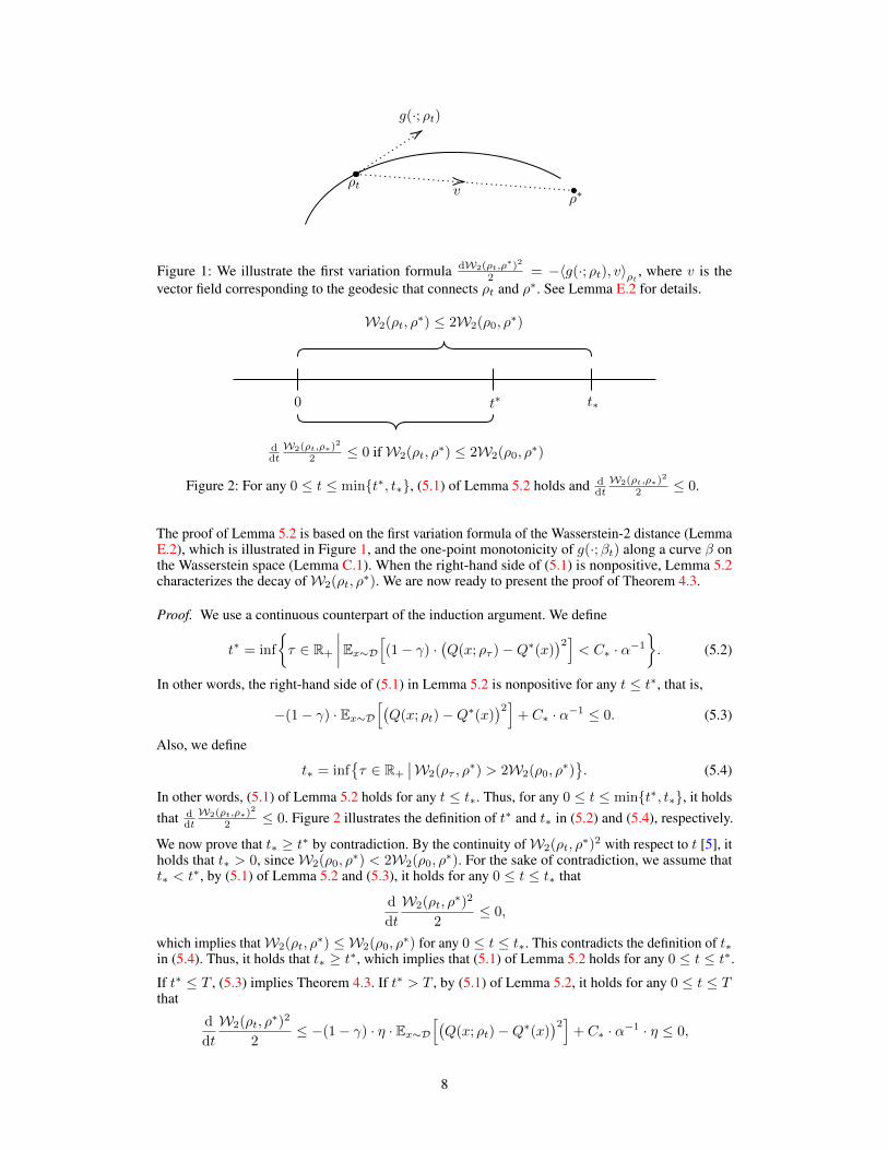
Figure 1: We illustrate the first variation formula dW2(⇢t,⇢⇤)2
2 = �hg(·; ⇢t), vi⇢t, where v is the
vector field corresponding to the geodesic that connects ⇢t and ⇢⇤. See Lemma E.2 for details.
0 t⇤ t⇤
W2(⇢t, ⇢⇤) 2W2(⇢0, ⇢⇤)
ddt
W2(⇢t,⇢⇤)2
2 0 if W2(⇢t, ⇢⇤) 2W2(⇢0, ⇢⇤)
Figure 2: For any 0 t min{t⇤, t⇤}, (5.1) of Lemma 5.2 holds and ddt
W2(⇢t,⇢⇤)2
2 0.
The proof of Lemma 5.2 is based on the first variation formula of the Wasserstein-2 distance (LemmaE.2), which is illustrated in Figure 1, and the one-point monotonicity of g(·;�t) along a curve � onthe Wasserstein space (Lemma C.1). When the right-hand side of (5.1) is nonpositive, Lemma 5.2characterizes the decay of W2(⇢t, ⇢⇤). We are now ready to present the proof of Theorem 4.3.
Proof. We use a continuous counterpart of the induction argument. We define
t⇤ = inf
⇢⌧ 2 R+
����Ex⇠D
h(1� �) ·
�Q(x; ⇢⌧ )�Q
⇤(x)�2i
< C⇤ · ↵�1
�. (5.2)
In other words, the right-hand side of (5.1) in Lemma 5.2 is nonpositive for any t t⇤, that is,
�(1� �) · Ex⇠D
h�Q(x; ⇢t)�Q
⇤(x)�2i
+ C⇤ · ↵�1 0. (5.3)
Also, we define
t⇤ = inf�⌧ 2 R+
��W2(⇢⌧ , ⇢⇤) > 2W2(⇢0, ⇢
⇤) . (5.4)
In other words, (5.1) of Lemma 5.2 holds for any t t⇤. Thus, for any 0 t min{t⇤, t⇤}, it holdsthat d
dtW2(⇢t,⇢⇤)
2
2 0. Figure 2 illustrates the definition of t⇤ and t⇤ in (5.2) and (5.4), respectively.
We now prove that t⇤ � t⇤ by contradiction. By the continuity of W2(⇢t, ⇢⇤)2 with respect to t [5], it
holds that t⇤ > 0, since W2(⇢0, ⇢⇤) < 2W2(⇢0, ⇢⇤). For the sake of contradiction, we assume thatt⇤ < t
⇤, by (5.1) of Lemma 5.2 and (5.3), it holds for any 0 t t⇤ that
d
dt
W2(⇢t, ⇢⇤)2
2 0,
which implies that W2(⇢t, ⇢⇤) W2(⇢0, ⇢⇤) for any 0 t t⇤. This contradicts the definition of t⇤in (5.4). Thus, it holds that t⇤ � t
⇤, which implies that (5.1) of Lemma 5.2 holds for any 0 t t⇤.
If t⇤ T , (5.3) implies Theorem 4.3. If t⇤ > T , by (5.1) of Lemma 5.2, it holds for any 0 t T
thatd
dt
W2(⇢t, ⇢⇤)2
2 �(1� �) · ⌘ · Ex⇠D
h�Q(x; ⇢t)�Q
⇤(x)�2i
+ C⇤ · ↵�1 · ⌘ 0,
8
which further implies that
Ex⇠D
h�Q(x; ⇢t)�Q
⇤(x)�2i �(1� �)�1 · ⌘�1 · d
dt
W2(⇢t, ⇢⇤)2
2+
C⇤(1� �) · ↵ . (5.5)
Upon telescoping (5.5) and setting ⌘ = ↵�2, we obtain that
inft2[0,T ]
ED
h�Q(x; ⇢t)�Q
⇤(x)�2i
T�1 ·
Z T
0Ex⇠D
h�Q(x; ⇢t)�Q
⇤(x)�2i
dt
1/2 · (1� �)�1 · ⌘�1 · T�1 · W2(⇢0, ⇢⇤)2 + C⇤ · (1� �)�1 · ↵�1
1/2 · (1� �)�1 · D2 · T�1 + C⇤ · (1� �)�1 · ↵�1,
where the last inequality follows from the fact that ⌘ = ↵�2 and (iii) of Lemma 5.1. Thus, we
complete the proof of Theorem 4.3.
6 Extension to Q-Learning and Policy Improvement
In §B, we extend our analysis of TD to Q-learning and soft Q-learning for policy improvement. In§B.1, we introduce Q-learning and its mean-field limit. In §B.2, we establish the global optimalityand convergence of Q-learning. In §B.3, we further extend our analysis to soft Q-learning, which isequivalent to a variant of policy gradient [37, 57, 58, 61].
Broader Impact
The popularity of RL creates a responsibility for researchers to design algorithms with guaranteedsafety and robustness, which rely on their stability and convergence. In this paper, we providea theoretical understanding of the global optimality and convergence of the TD and Q-learningwith neural network parameterization. We believe that our work is an important step forward inthe algorithm design of RL in emerging high-stakes applications, such as autonomous driving,personalized medicine, power systems, and robotics.
References
[1] Agazzi, A. and Lu, J. (2019). Temporal-difference learning for nonlinear value function approx-imation in the lazy training regime. arXiv preprint arXiv:1905.10917.
[2] Allen-Zhu, Z., Li, Y. and Liang, Y. (2018). Learning and generalization in overparameterizedneural networks, going beyond two layers. arXiv preprint arXiv:1811.04918.
[3] Allen-Zhu, Z., Li, Y. and Song, Z. (2018). A convergence theory for deep learning via over-parameterization. arXiv preprint arXiv:1811.03962.
[4] Ambrosio, L. and Gigli, N. (2013). A users guide to optimal transport. In Modelling andOptimisation of Flows on Networks. Springer, 1–155.
[5] Ambrosio, L., Gigli, N. and Savare, G. (2008). Gradient flows: In metric spaces and in thespace of probability measures. Springer.
[6] Araujo, D., Oliveira, R. I. and Yukimura, D. (2019). A mean-field limit for certain deep neuralnetworks. arXiv preprint arXiv:1906.00193.
[7] Arora, S., Du, S. S., Hu, W., Li, Z., Salakhutdinov, R. R. and Wang, R. (2019). On exact com-putation with an infinitely wide neural net. In Advances in Neural Information ProcessingSystems.
[8] Arora, S., Du, S. S., Hu, W., Li, Z. and Wang, R. (2019). Fine-grained analysis of optimiza-tion and generalization for overparameterized two-layer neural networks. arXiv preprintarXiv:1901.08584.
9
[9] Bai, Y. and Lee, J. D. (2019). Beyond linearization: On quadratic and higher-order approxima-tion of wide neural networks. arXiv preprint arXiv:1910.01619.
[10] Baird, L. (1995). Residual algorithms: Reinforcement learning with function approximation. InInternational Conference on Machine Learning.
[11] Barron, A. R. (1993). Universal approximation bounds for superpositions of a sigmoidalfunction. IEEE Transactions on Information Theory, 39 930–945.
[12] Bengio, Y. (2012). Deep learning of representations for unsupervised and transfer learning. InICML Workshop on Unsupervised and Transfer Learning.
[13] Bertsekas, D. P. (2019). Feature-based aggregation and deep reinforcement learning: A surveyand some new implementations. IEEE/CAA Journal of Automatica Sinica, 6 1–31.
[14] Bhandari, J., Russo, D. and Singal, R. (2018). A finite time analysis of temporal differencelearning with linear function approximation. arXiv preprint arXiv:1806.02450.
[15] Bhatnagar, S., Precup, D., Silver, D., Sutton, R. S., Maei, H. R. and Szepesvari, C. (2009). Con-vergent temporal-difference learning with arbitrary smooth function approximation. In Advancesin Neural Information Processing Systems.
[16] Borkar, V. S. (2009). Stochastic approximation: A dynamical systems viewpoint. Springer.
[17] Borkar, V. S. and Meyn, S. P. (2000). The ODE method for convergence of stochastic approxi-mation and reinforcement learning. SIAM Journal on Control and Optimization, 38 447–469.
[18] Boyan, J. A. and Moore, A. W. (1995). Generalization in reinforcement learning: Safely ap-proximating the value function. In Advances in Neural Information Processing Systems.
[19] Brandfonbrener, D. and Bruna, J. (2019). Geometric insights into the convergence of nonlinearTD learning. arXiv preprint arXiv:1905.12185.
[20] Brandfonbrener, D. and Bruna, J. (2019). On the expected dynamics of nonlinear TD learning.arXiv preprint arXiv:1905.12185.
[21] Cai, Q., Yang, Z., Lee, J. D. and Wang, Z. (2019). Neural temporal-difference learning con-verges to global optima. In Advances in Neural Information Processing Systems.
[22] Cao, Y. and Gu, Q. (2019). Generalization bounds of stochastic gradient descent for wide anddeep neural networks. arXiv preprint arXiv:1905.13210.
[23] Chen, Z., Cao, Y., Gu, Q. and Zhang, T. (2020). Mean-field analysis of two-layer neural net-works: Non-asymptotic rates and generalization bounds. arXiv preprint arXiv:2002.04026.
[24] Chen, Z., Cao, Y., Zou, D. and Gu, Q. (2019). How much over-parameterization is sufficient tolearn deep ReLU networks? arXiv preprint arXiv:1911.12360.
[25] Chen, Z., Zhang, S., Doan, T. T., Maguluri, S. T. and Clarke, J.-P. (2019). Performance of q-learning with linear function approximation: Stability and finite-time analysis. arXiv preprintarXiv:1905.11425.
[26] Chizat, L. and Bach, F. (2018). A note on lazy training in supervised differentiable programming.arXiv preprint arXiv:1812.07956.
[27] Chizat, L. and Bach, F. (2018). On the global convergence of gradient descent for over-parameterized models using optimal transport. In Advances in Neural Information ProcessingSystems.
[28] Conway, J. B. (2019). A course in functional analysis, vol. 96. Springer.
[29] Dalal, G., Szorenyi, B., Thoppe, G. and Mannor, S. (2018). Finite sample analyses for TD(0)with function approximation. In AAAI Conference on Artificial Intelligence.
[30] Daniely, A. (2017). SGD learns the conjugate kernel class of the network. In Advances inNeural Information Processing Systems.
10
[31] Dann, C., Neumann, G. and Peters, J. (2014). Policy evaluation with temporal differences: Asurvey and comparison. Journal of Machine Learning Research, 15 809–883.
[32] Du, S. S., Lee, J. D., Li, H., Wang, L. and Zhai, X. (2018). Gradient descent finds global minimaof deep neural networks. arXiv preprint arXiv:1811.03804.
[33] Du, S. S., Zhai, X., Poczos, B. and Singh, A. (2018). Gradient descent provably optimizesover-parameterized neural networks. arXiv preprint arXiv:1810.02054.
[34] Fang, C., Dong, H. and Zhang, T. (2019). Over parameterized two-level neural networks canlearn near optimal feature representations. arXiv preprint arXiv:1910.11508.
[35] Fang, C., Gu, Y., Zhang, W. and Zhang, T. (2019). Convex formulation of overparameterizeddeep neural networks. arXiv preprint arXiv:1911.07626.
[36] Geist, M. and Pietquin, O. (2013). Algorithmic survey of parametric value function approxima-tion. IEEE Transactions on Neural Networks and Learning Systems, 24 845–867.
[37] Haarnoja, T., Tang, H., Abbeel, P. and Levine, S. (2017). Reinforcement learning with deepenergy-based policies. In International Conference on Machine Learning.
[38] Harker, P. T. and Pang, J.-S. (1990). Finite-dimensional variational inequality and nonlinearcomplementarity problems: A survey of theory, algorithms and applications. MathematicalProgramming, 48 161–220.
[39] He, J., Chen, J., He, X., Gao, J., Li, L., Deng, L. and Ostendorf, M. (2015). Deep reinforcementlearning with a natural language action space. arXiv preprint arXiv:1511.04636.
[40] Hinton, G. (1986). Learning distributed representations of concepts. In Annual Conference ofCognitive Science Society.
[41] Holte, J. M. (2009). Discrete Gronwall lemma and applications. In MAA-NCS Meeting at theUniversity of North Dakota, vol. 24.
[42] Jaakkola, T., Jordan, M. I. and Singh, S. P. (1994). Convergence of stochastic iterative dynamicprogramming algorithms. In Advances in Neural Information Processing Systems.
[43] Jacot, A., Gabriel, F. and Hongler, C. (2018). Neural tangent kernel: Convergence and general-ization in neural networks. In Advances in Neural Information Processing Systems.
[44] Javanmard, A., Mondelli, M. and Montanari, A. (2019). Analysis of a two-layer neural networkvia displacement convexity. arXiv preprint arXiv:1901.01375.
[45] Ji, Z. and Telgarsky, M. (2019). Polylogarithmic width suffices for gradient descent to achievearbitrarily small test error with shallow ReLU networks. arXiv preprint arXiv:1909.12292.
[46] Konda, V. R. and Tsitsiklis, J. N. (2000). Actor-critic algorithms. In Advances in NeuralInformation Processing Systems.
[47] Kushner, H. and Yin, G. G. (2003). Stochastic approximation and recursive algorithms andapplications. Springer.
[48] Lakshminarayanan, C. and Szepesvari, C. (2018). Linear stochastic approximation: How fardoes constant step-size and iterate averaging go? In International Conference on ArtificialIntelligence and Statistics.
[49] LeCun, Y., Bengio, Y. and Hinton, G. (2015). Deep learning. Nature, 521 436–444.
[50] Lee, J., Xiao, L., Schoenholz, S. S., Bahri, Y., Sohl-Dickstein, J. and Pennington, J. (2019).Wide neural networks of any depth evolve as linear models under gradient descent. arXivpreprint arXiv:1902.06720.
[51] Levine, S., Finn, C., Darrell, T. and Abbeel, P. (2016). End-to-end training of deep visuomotorpolicies. Journal of Machine Learning Research, 17 1334–1373.
11
[52] Li, Y. and Liang, Y. (2018). Learning overparameterized neural networks via stochastic gradientdescent on structured data. In Advances in Neural Information Processing Systems.
[53] Mei, S., Misiakiewicz, T. and Montanari, A. (2019). Mean-field theory of two-layers neuralnetworks: Dimension-free bounds and kernel limit. arXiv preprint arXiv:1902.06015.
[54] Mei, S., Montanari, A. and Nguyen, P.-M. (2018). A mean field view of the landscape of two-layer neural networks. Proceedings of the National Academy of Sciences, 115 E7665–E7671.
[55] Melo, F. S., Meyn, S. P. and Ribeiro, M. I. (2008). An analysis of reinforcement learning withfunction approximation. In International Conference on Machine Learning.
[56] Mnih, V., Kavukcuoglu, K., Silver, D., Rusu, A. A., Veness, J., Bellemare, M. G., Graves, A.,Riedmiller, M., Fidjeland, A. K., Ostrovski, G. et al. (2015). Human-level control through deepreinforcement learning. Nature, 518 529–533.
[57] Nachum, O., Norouzi, M., Xu, K. and Schuurmans, D. (2017). Bridging the gap between valueand policy based reinforcement learning. In Advances in Neural Information ProcessingSystems.
[58] O’Donoghue, B., Munos, R., Kavukcuoglu, K. and Mnih, V. (2016). Combining policy gradientand Q-learning. arXiv preprint arXiv:1611.01626.
[59] Otto, F. and Villani, C. (2000). Generalization of an inequality by Talagrand and links with thelogarithmic Sobolev inequality. Journal of Functional Analysis, 173 361–400.
[60] Pinkus, A. (1999). Approximation theory of the MLP model in neural networks. Acta Numerica,8 143–195.
[61] Schulman, J., Chen, X. and Abbeel, P. (2017). Equivalence between policy gradients and softQ-learning. arXiv preprint arXiv:1704.06440.
[62] Sirignano, J. and Spiliopoulos, K. (2019). Asymptotics of reinforcement learning with neuralnetworks. arXiv preprint arXiv:1911.07304.
[63] Srikant, R. and Ying, L. (2019). Finite-time error bounds for linear stochastic approximationand TD learning. arXiv preprint arXiv:1902.00923.
[64] Sutton, R. S. (1988). Learning to predict by the methods of temporal differences. MachineLearning, 3 9–44.
[65] Sutton, R. S. and Barto, A. G. (2018). Reinforcement learning: An introduction. MIT press.
[66] Sznitman, A.-S. (1991). Topics in propagation of chaos. In Ecole d’Ete de Probabilites deSaint-Flour XIX1989. Springer, 165–251.
[67] Tsitsiklis, J. N. and Van Roy, B. (1997). Analysis of temporal-diffference learning with functionapproximation. In Advances in Neural Information Processing Systems.
[68] Villani, C. (2003). Topics in optimal transportation. American Mathematical Society.
[69] Villani, C. (2008). Optimal transport: Old and new. Springer.
[70] Wainwright, M. J. (2019). High-dimensional statistics: A non-asymptotic viewpoint. CambridgeUniversity Press.
[71] Watkins, C. and Dayan, P. (1992). Q-learning. Machine Learning, 8 279–292.
[72] Wei, C., Lee, J. D., Liu, Q. and Ma, T. (2019). Regularization matters: Generalization and opti-mization of neural nets vs their induced kernel. In Advances in Neural Information ProcessingSystems.
[73] Williams, R. J. (1992). Simple statistical gradient-following algorithms for connectionist rein-forcement learning. Machine Learning, 8 229–256.
12
[74] Xu, T., Zou, S. and Liang, Y. (2019). Two time-scale off-policy TD learning: Non-asymptoticanalysis over Markovian samples. In Advances in Neural Information Processing Systems.
[75] Yosinski, J., Clune, J., Bengio, Y. and Lipson, H. (2014). How transferable are features in deepneural networks? In Advances in Neural Information Processing Systems.
[76] Zou, D., Cao, Y., Zhou, D. and Gu, Q. (2018). Stochastic gradient descent optimizes over-parameterized deep ReLU networks. arXiv preprint arXiv:1811.08888.
[77] Zou, D. and Gu, Q. (2019). An improved analysis of training over-parameterized deep neuralnetworks. In Advances in Neural Information Processing Systems.
[78] Zou, S., Xu, T. and Liang, Y. (2019). Finite-sample analysis for SARSA and Q-learning withlinear function approximation. arXiv preprint arXiv:1902.02234.
13