Embed Size (px)
Citation preview
Can the Two-Time Interpretation of QuantumMechanics Solve the Measurement Problem?
Katie RobertsonFebruary 2017
Forthcoming in Studies in History and Philosophy of Science Part B - Studies in Historyand Philosophy of Modern Physics
Abstract
Over many years, Aharonov and co-authors have proposed a new interpretationof quantum mechanics: the two-time interpretation. This interpretation assignstwo wavefunctions to a system, one of which propagates forwards in time andthe other backwards. In this paper, I argue that this interpretation does notsolve the measurement problem. In addition, I argue that it is neither necessarynor sufficient to attribute causal power to the backwards-evolving wavefunction〈Φ| and thus its existence should be denied, contra the two-time interpretation.Finally, I follow Vaidman in giving an epistemological reading of 〈Φ|.
1
1 Introduction
It is uncontroversial to say that there is no (global) consensus as to which inter-
pretation of quantum mechanics should be adopted. In this paper, I will evaluate
a new interpretation proposed by Aharonov, Gruss [2], Cohen and Landsberger [9]
called the Two-Time Interpretation (TTI)1, which claims to be local, determin-
istic and to predict and explain novel phenomena. I will concentrate on whether
this interpretation solves the measurement problem: since a prerequisite for join-
ing the panoply of interpretations of quantum mechanics (QM) is to solve the
measurement problem. I will argue that it does not.
The measurement problem arises as follows. When a measuring device2 mea-
sures a system initially in the state |ΨS〉 = α |↑x〉 + β |↓x〉, the joint state of the
system and apparatus evolves, by linearity, to
|ΦS+A〉 = α |↑x〉S |up〉A + β |↓x〉S |down〉A . (1)
The macroscopic measuring device is now entangled with the system and the
composite system is in a superposition with respect to the product state basis.
However, we never experience macroscopic superpositions, such as measuring de-
vices pointing at both ‘up’ and ‘down’. Rather, the measuring device will appear
to display a single definite outcome.
In practice, in order to get empirical content from the formalism we apply
a set of rules for measurement (sometimes called ‘the measurement algorithm’
[43]): write the state in the basis of the measured quantity/observable, and the
pointer, αi |ai〉 |Ai〉, and then interpret |α1|2 as the probability (Pr) of finding
state |a1〉. In the case above, the measuring device is either found in the state
|up〉 with Pr = |α|2 or |down〉 with Pr = |β|2. Thus one way of describing the
measurement problem is to say that this algorithm lacks a justification and ‘to
solve the measurement problem we need to give a well-formulated theory which
explains the success of the measurement algorithm’ [42].
In this paper I evaluate whether the TTI can solve this measurement problem.
As the TTI arises from a particular reading of the two-state vector formalism
(TSVF), I will first, in section 2, discuss the TSVF. In section 3, I outline the key
tenets of the TTI as well as its proposed solution to the measurement problem.
1The two papers cited explicitly expound the TTI, but other papers such as [3] and [4] hint at it,since — as will become apparent shortly — the TTI naturally arises out of a wider research programme.
2As usual, we model a measurement by a composite unitary operator U that takes the measuringdevice to one of several distinguishable (orthogonal) states depending on the system’s state. Thus, ameasuring apparatus that measures spin-x behaves as follows:
U |↑x〉S |ready〉A → |↑x〉S |up〉A
U |↓x〉S |ready〉A → |↓x〉S |down〉A .
2
Section 4 first investigates whether the TTI explains the success of the measure-
ment algorithm, and then whether it is well-formulated. In section 5, I argue that
there are further problems facing this interpretation, and in section 6 I advocate
an alternative reading of the situation.
2 What is the two-state vector formalism?
The two-state vector formalism (TVSF)[4, 1] alters the traditional formalism of
QM by assigning an additional state vector 〈Φ| to a system, as well as the usual
state vector, |Ψ〉. The latter state vector |Ψ(t0)〉 unitarily evolves according to the
Schrodinger equation, under U . However, the state 〈Φ(t1)| evolves unitarily back-
wards in time under U † and thus is called the ‘backwards-evolving state vector’.3
Combined they form the two-state vector,
〈Φ| |Ψ〉 (2)
which also evolves unitarily. The philosophical motivation behind TSVF is to re-
move the time asymmetry implicit in the standard QM formalism, which Aharonov
et al. [11] see as originating in the usual conception of state, rather than being
inherent in QM. Using final and initial conditions is more time-symmetric than
just initial conditions.
The TSVF is not an interpretation of QM: rather it is a mathematical for-
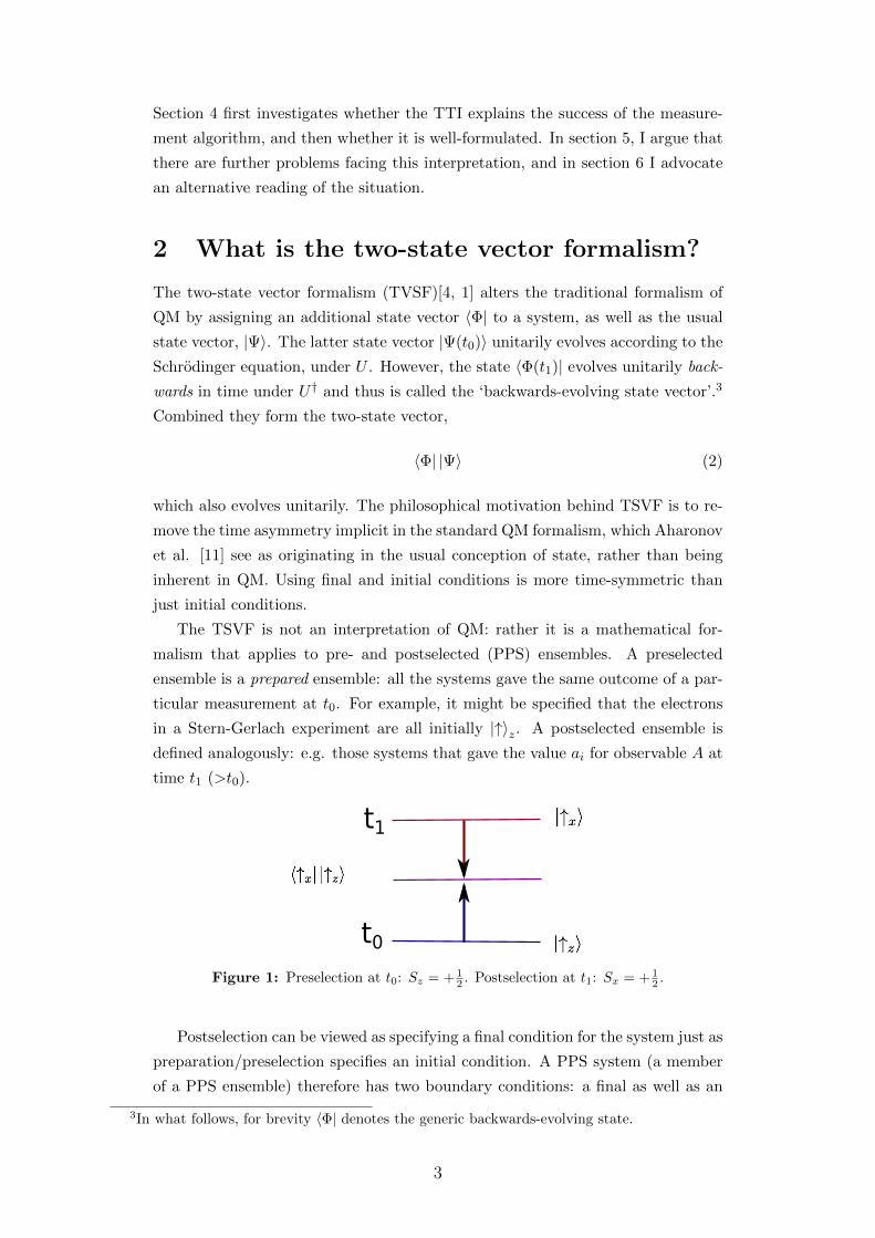
malism that applies to pre- and postselected (PPS) ensembles. A preselected
ensemble is a prepared ensemble: all the systems gave the same outcome of a par-
ticular measurement at t0. For example, it might be specified that the electrons
in a Stern-Gerlach experiment are all initially |↑〉z. A postselected ensemble is
defined analogously: e.g. those systems that gave the value ai for observable A at
time t1 (>t0).
t0
t1
Figure 1: Preselection at t0: Sz = + 12 . Postselection at t1: Sx = + 1
2 .
Postselection can be viewed as specifying a final condition for the system just as
preparation/preselection specifies an initial condition. A PPS system (a member
of a PPS ensemble) therefore has two boundary conditions: a final as well as an
3In what follows, for brevity 〈Φ| denotes the generic backwards-evolving state.
3

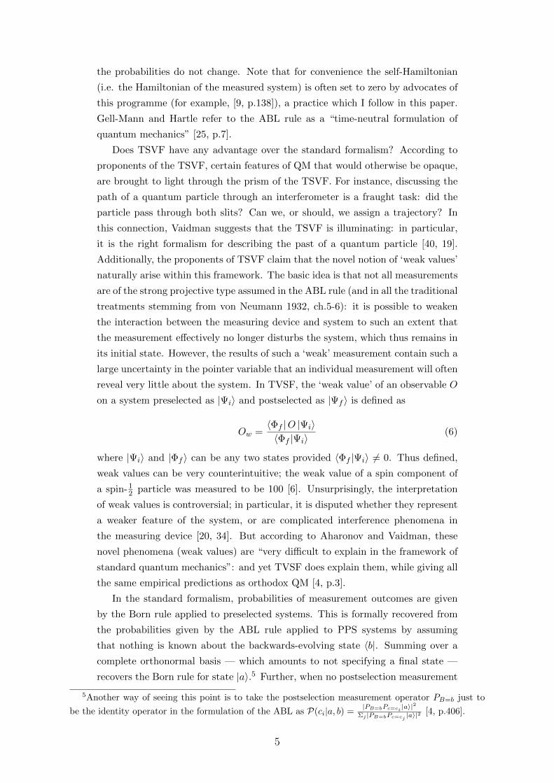
t0
t1
Sx=+1/2
Figure 2: An intermediate measurementof Sx in the period t0 <t <t1 finds theeigenvalue + 1
2 with Pr = 1.
t0
t1
Sz=+1\2
Figure 3: An intermediate measurementof Sz in the period t0 <t <t1 finds theeigenvalue + 1
2 with Pr = 1.
initial condition.4 These boundary conditions (and therefore the two-state vector)
are defined by measurement outcomes, as shown in Figure 1. We envisage that
measurements are made on the system in the period t0 <t <t1, as shown in Figures
2 and 3. Note how the situation differs from classical mechanics: classically,
if we know the initial condition and the dynamics (the Hamiltonian) then the
information contained in the final condition is redundant. However, in QM there
is, for some measurements, no way even in principle to predict the result. Thus,
specifying a final condition gives us more information about the system than just
an initial condition.
Next, a method of determining the probabilities of outcomes of different mea-
surements on PPS systems is needed. This is given by the Aharonov, Bergmann
and Lebowitz (ABL) rule [1] which tells us, given an initial state |a〉 and a fi-
nal state |b〉, the probability that an intermediate projective measurement of the
non-degenerate operator C yields eigenvalue ci. We begin with the formula
P(ci|a, b) =P(b|ci)P(ci|a)
ΣjP(b|cj)P(cj |a). (3)
Note that this expression is derived from the probability calculus: the Hamiltonian
is set to zero and the only physical assumption is that ci screens off b from a, i.e.
the intermediate measurement is projective. Using Pr(g|f) = | 〈g|f〉 |2, we find:
P(ci|a, b) =| 〈b|ci〉 〈ci|a〉 |2
Σj | 〈b|cj〉 〈cj |a〉 |2. (4)
In the case of non-trivial time evolution, the ABL rule becomes:
P(ci|a, b) =| 〈b|U(tb, t) |ci〉 〈ci|U(t, ta) |a〉 |2
Σj | 〈b|U(tb, t) |cj〉 〈cj |U(t, ta) |a〉 |2. (5)
For the PPS system shown in Figures 1-3, the ABL rule gives Pr = 1 for
an intermediate result of Sz = +12 and likewise for Sx = +1
2 . For Sy = +12 ,
Pr = 12 . The ABL rule is time-symmetric in the sense that, if the initial and final
states are exchanged, then provided the Hamiltonian is time-reversal invariant,
4In practice, measurements on postselected ensembles involve doing a measurement on the wholepreselected ensemble, then performing a selective measurement and discarding the results for systemsthat do not pass the postselection.
4
the probabilities do not change. Note that for convenience the self-Hamiltonian
(i.e. the Hamiltonian of the measured system) is often set to zero by advocates of
this programme (for example, [9, p.138]), a practice which I follow in this paper.
Gell-Mann and Hartle refer to the ABL rule as a “time-neutral formulation of
quantum mechanics” [25, p.7].
Does TSVF have any advantage over the standard formalism? According to
proponents of the TSVF, certain features of QM that would otherwise be opaque,
are brought to light through the prism of the TSVF. For instance, discussing the
path of a quantum particle through an interferometer is a fraught task: did the
particle pass through both slits? Can we, or should, we assign a trajectory? In
this connection, Vaidman suggests that the TSVF is illuminating: in particular,
it is the right formalism for describing the past of a quantum particle [40, 19].
Additionally, the proponents of TSVF claim that the novel notion of ‘weak values’
naturally arise within this framework. The basic idea is that not all measurements
are of the strong projective type assumed in the ABL rule (and in all the traditional
treatments stemming from von Neumann 1932, ch.5-6): it is possible to weaken
the interaction between the measuring device and system to such an extent that
the measurement effectively no longer disturbs the system, which thus remains in
its initial state. However, the results of such a ‘weak’ measurement contain such a
large uncertainty in the pointer variable that an individual measurement will often
reveal very little about the system. In TVSF, the ‘weak value’ of an observable O
on a system preselected as |Ψi〉 and postselected as |Ψf 〉 is defined as
Ow =〈Φf |O |Ψi〉〈Φf |Ψi〉
(6)
where |Ψi〉 and |Φf 〉 can be any two states provided 〈Φf |Ψi〉 6= 0. Thus defined,
weak values can be very counterintuitive; the weak value of a spin component of
a spin-12 particle was measured to be 100 [6]. Unsurprisingly, the interpretation
of weak values is controversial; in particular, it is disputed whether they represent
a weaker feature of the system, or are complicated interference phenomena in
the measuring device [20, 34]. But according to Aharonov and Vaidman, these
novel phenomena (weak values) are “very difficult to explain in the framework of
standard quantum mechanics”: and yet TVSF does explain them, while giving all
the same empirical predictions as orthodox QM [4, p.3].
In the standard formalism, probabilities of measurement outcomes are given
by the Born rule applied to preselected systems. This is formally recovered from
the probabilities given by the ABL rule applied to PPS systems by assuming
that nothing is known about the backwards-evolving state 〈b|. Summing over a
complete orthonormal basis — which amounts to not specifying a final state —
recovers the Born rule for state |a〉.5 Further, when no postselection measurement
5Another way of seeing this point is to take the postselection measurement operator PB=b just to
be the identity operator in the formulation of the ABL as P(ci|a, b) =|PB=bPc=ci
|a〉|2
Σj |PB=bPc=cj|a〉|2 [4, p.406].
5
is made, the weak value reduces to the expectation value of the observable con-
cerned. Thus, the standard formalism is recovered by making the final condition
one that assumes no postselection. Aharonov and Rohrlich claim this choice of
boundary conditions is the source of the time-asymmetry in standard QM: “by
imposing an initial but not a final boundary condition, we have already sent the
arrow of time flying” [3, p.137].
Next, I will consider the ‘ontological’ interpretation of the two-state vector.
3 The two-time interpretation (TTI)
Aharonov et al. introduce the Two-Time interpretation (TTI) and claim it is
a deterministic, local and ontological interpretation of QM, that also solves the
measurement problem [2, 9]. In section 3.1, I will consider the status of the
backwards-evolving wavefunction within TTI and whether TTI is a hidden variable
theory, before explicating their reasons for thinking it is local and deterministic.
Then, in section 3.2, I will review their proposed solution to the measurement
problem.
3.1 The interpretation of 〈Φ|This interpretation claims that there really is a backwards-evolving state vector
〈Φ| (just as much as there is a forwards-evolving state |Ψ〉). Therefore, at every
moment in time there is a two-state vector (and therefore two Hilbert spaces)
associated with the system. Ordinarily |↑〉x is taken to describe the system after a
projective measurement of Sx with outcome ‘up’ at t1. In TTI, 〈↑|x in Figure 1 de-
scribes the system even before the postselection measurement (Sx at t1). Further,
if 〈Φ| is on equal footing with the usual state vector |Ψ〉 and an ontological reading
of the quantum state is taken (as the TTI proposes6), then 〈Φ| has, presumably,
causal power. Thus, as might be expected from a time-symmetric theory, there
is retrocausality in the TTI [9, p.143]: “future and past are equally important in
determining the quantum state at intermediate times, and hence equally real” [18,
p.10].
This ontological interpretation of 〈Φ| in TTI goes beyond TSVF in two re-
spects. First, the role of 〈Φ| in the weak values formula (6) and the ABL rule (4)
does not require it to be assigned to the system at the earlier time t, t0 < t < t1.
In these formulas, one could consistently interpret it merely as the mathematical
dual of the vector that describes the system later at t1. Secondly, whilst mea-
surements on PPS systems may, prima facie, seem contrived or artificial because
6Aharonov and Gruss deny an epistemological interpretation which “pretends only to give a setof logical rules regarding our knowledge of reality, and does not attempt to explain any underlyingprocesses taking place” [2, p.2].
6

sometimes many intermediate measurement results must be discarded7, in fact in
the TTI the PPS ensemble is more fundamental than the PS ensemble. The seem-
ingly artificial nature of performing measurements on PPS systems stems simply
from our ignorance until time t1 of the backwards-evolving wavefunction, 〈Φ|. If
we somehow knew 〈Φ| before t1, we could perform the intermediate measurement
only on the systems that would later pass the postselection, and we would thus
not need to throw any intermediate measurement results away. Thus, the TTI
takes the PPS system to be the more complete and natural description of the
system even prior to the postselection measurement; systems have “an inherent
final boundary condition just as all systems have an initial boundary condition”
[9, p.135][26, p.11]. Thus, “in order to fully specify a system, one should not only
preselect, but also postselect a certain state using a projective measurement” [18,
p.10].
Now recall that if QM is a fundamental and universal theory, the quantum
state |Ψ〉S with which we usually describe a system S, is really just a factor
of a state |Ψ〉U = |ϕ〉S ⊗ |Ψ〉P ⊗ ... which describes the whole universe [9, 27].
Accordingly, this interpretation holds that, in addition to the initial quantum
state of the universe, there is a final quantum state of the universe, of which the
backwards-evolving state of S is just a part. Whilst the final state of the universe
is unknown, Aharonov et al. make some assumptions about its form.
These initial and final states of the universe are referred to by Aharonov and
Gruss as the ‘history vector’ |ΨHIS〉 and the ‘destiny vector’ 〈ΦDES | respectively
and the latter records the result of every measurement ever made [2, p.3]. As
the only type of time evolution is unitary, no information is lost. As well as the
two-state vector 〈Φ| |Ψ〉, the formalism defines the two-time density matrix, which
in the particular case of 〈ΦDES | and |ΨHIS〉 is,
ρ = |ΨHIS〉 〈ΦDES | . (7)
Of course, since 〈ΦDES | and |ΨHIS〉 are, a priori, unrelated kets, ρ in (7) is
not hermitian — unlike usual density matrices. For more details on this novel
conception of state, cf. [10, p.13], which also formulates this novel ‘two-time’
conception of state in the Heisenberg representation.8
I now turn to how the TTI relates to three key topics: hidden variables, non-
locality and determinism.
7Note, however, that it is possible, according to [8], to perform a weak measurement on a singleparticle, where all measurement results are used. My thanks to an anonymous referee for bringing thisexample to my attention.
8Note, however, that the formulation in [10] diverges from the TTI outlined in this paper, since theTTI is usually advertised as a local theory (cf. section 3.1.2 below), whereas [10] involves a form ofnon-locality that goes beyond the familiar QM-theoretic non-separability of entangled systems. This,more extreme, dynamical non-locality is manifest, for example, when a quantum particle is describedas passing through one slit but exchanging a form of momentum non-locally with the other slit.
7
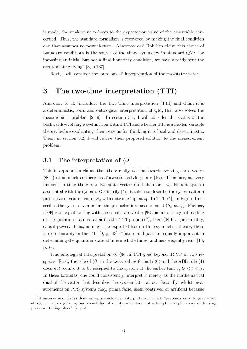
3.1.1 Is TTI a hidden variable theory?
Is TTI a hidden variable theory like the pilot-wave theory (Bohmian mechanics)?
Whilst the backwards-evolving wavefunction 〈Φ| exists at every instant of time,
it is hidden from us. Only at the later time t1 in Figures 2 and 3 are we able to
discover that 〈Φ| = 〈↑|x in the interval t0 < t < t1. Indeed, if we were able to
access 〈Φ| prior to the postselection measurement, superluminal signalling would
be possible, contradicting the no-signalling theorem (see [9, p.142]). Therefore,
in the sense that it exists (according to TTI) and yet one is ignorant of it, 〈Φ|is a hidden variable. And as in other hidden variable theories, the statistical
features of quantum mechanics stem from our ignorance of the hidden variables.
Thus, probability in the TTI has an epistemic, rather than ontic, nature; “the
probabilistic nature of quantum events can be thought of as stemming from our
ignorance of the backwards-evolving state, reintroducing the classical concept of
probability as a measure of our knowledge” [9, p.134].
However, TTI is not a hidden variable theory in the traditional sense. Usually a
hidden variable theory claims that the system has definite values of an observable
even when it is not in an eigenstate of that observable (or in the case of TTI,
is neither in a forwards-evolving eigenstate nor a backwards-evolving eigenstate).
But in the TTI, there are no extra value assignments in this sense.
3.1.2 Is the TTI local?
Aharonov and Gruss explicitly claim that the TTI is a local theory [2, p.1]. Of
course, the predictions of QM violate Bell’s inequalities, and so it is commonly
claimed that any hidden variables must be non-local. This raises the question:
how does the TTI square with Bell’s theorem?
Whilst the proponents of the TTI do not explicitly relate their novel conception
of state, 〈Φ| |Ψ〉 as in equation 2 or ρ as in equation (7), to the hidden variable λ
mentioned in the assumptions of Bell’s theorem, I think it is clear [7] that they
deny that the settings in the two wings of the EPR-Bell apparatus are independent
of each other, simply because the measurement outcomes are ‘recorded’ in 〈Φ|DESand so the apparatus settings that Alice and Bob choose is encoded in 〈Φ|DES .
Thus these settings are not independent.9
More generally, setting aside the exact formulation of assumptions of a Bell
theorem: the question arises how should we understand ‘locality’ for a theory
which, like the TTI, involves retrocausality. Usually, locality requires that no
event can causally influence another event outside of its future lightcone. In the
TTI, the natural suggestion is therefore that locality requires that no event can
9That is, in terms of Shimony’s jargon [33] of parameter independence and outcome independence:it seems to me that, taking the TTI’s novel state ρ to be the schematic hidden variable λ in Shimony’sconditions, TTI violates parameter independence. Nevertheless, despite this parameter dependence, westill have the no-signalling property.
8
causally influence another event outside of its future or past lightcone.
3.1.3 Is the TTI deterministic?
Aharonov et al. say that the TTI is a deterministic theory, albeit in a special
way. To assess this claim, recall the core idea of determinism: a theory is a set of
models T = {Mi}, where Mi is a possible history of the system i.e. an assignment
at each time of a state to the system; and T is deterministic if and only if, for all
M1 and M2 in T , if M1 and M2 agree on the state of the system at some given
time t, then they agree on the system’s state for all future times [17].
From this definition, it is clear that whether a theory counts as deterministic
will very much depend on the conception of ‘state’. To avoid trivially ensuring
determinism, the information encoded in a ‘state’ must be intrinsic to the time
in question. To take an everyday example (following [17]): obviously, ‘Fred was
fatally wounded at noon’ logically implies that Fred later died. But it does not
imply that the processes leading to Fred’s death were deterministic. They might
well have been stochastic, and at the time of the wound, his death might even
have been improbable. Thus, the apparent determinism in this case is ‘cheating’:
it arises from encoding in a statement about noon (an attribution of a ‘state’ at
noon, i.e. ‘fatally wounded’) information about the future (Fred’s later demise).10
Thus, whether QM is a deterministic theory will depend how the ‘state of
a system’ is defined and this is entwined with one’s view of the measurement
problem [21]. Insofar as there is no consensus on the measurement problem, there
is no consensus as to whether QM is deterministic. For example, in the textbook
spontaneous collapse QM theory, the state is the wavefunction and this theory is
indeterministic. By contrast, in the pilot-wave theory the state of the system is
described by the wavefunction and the particles’ position, and consequently the
theory is deterministic.
What about the TTI? Aharonov et al. claim that the theory is ‘two-time
deterministic’: “the state of the system at any given time is completely determined
by its two-state at any single time in the course of history” [9, p.142]. Thus, if the
notion of state is the two-state vector 〈Φ| |Ψ〉 of equation (2) rather than usual
state vector |Ψ〉, then, they claim, the TTI is deterministic, like the pilot-wave
theory. This has an epistemological construal akin to the pilot-wave theory. In
the pilot-wave theory, were we to know the position of the particles in addition to
the wavefunction, then predictability of measurement outcomes would be restored.
Likewise, it seems that were we to know the generic backwards-evolving state 〈Φ|,the TTI claims we would know the measurement outcomes.
The new terminology ‘two-time determinism’ is important, since the TTI flouts
the standard definition given above: by defining the state as two-time state 〈Φ| |Ψ〉,10See [17] for discussion of natural conditions on the notion of state, in order to make determinism
nontrivial.
9
their notion, arguably, ‘looks ahead’ to the future in the same way that the descrip-
tion ‘fatally wounded’ does. In the last part of section 5, this claim of ‘two-time
determinism’ is explored further.
3.2 A review of TTI’s solution to the measurement
problem
For TTI to count as an interpretation of quantum theory, it must propose a reso-
lution to the measurement problem. The proponents of TTI describe the measure-
ment problem as arising from the ‘discrepancy’ [2, p.1] between the superpositions
that result from unitary evolution and single measurement outcomes. Here I re-
view their strategy for solving this problem [2, p.4] [9, p.139] [18, p.14].
We envisage that, using the notation from Section 1, the system, apparatus
and environment begin in the following state:
|Initial〉 = (a |↑〉+ b |↓〉)⊗ |ready〉 ⊗ |ε〉 , (8)
which unitarily evolves to
(a |↑〉 ⊗ |up〉+ b |↓〉 ⊗ |down〉)⊗ |ε〉 ; (9)
the measuring device then interacts with the environment, encoding the interfer-
ence in the environment in the usual decohering manner to
a |↑〉 ⊗ |up〉 ⊗ |εup〉+ b |↓〉 ⊗ |down〉 ⊗ |εdown〉 , (10)
where |εup〉 and |εdown〉 are orthogonal (or nearly so).
Next, the backwards-evolving final boundary condition of the entire system,
expressed as a bra is taken to be
〈Final| = 〈φ| ⊗ 〈up| ⊗ 〈εup| . (11)
Crucially, the state of the measuring device is chosen to be a single member
|up〉 of the measurement basis. But the particle could have been measured in the
interval between the initial time and the final time; and so it is in an arbitrary
state: |φ〉 = c |↑〉 + d |↓〉. Thus, in the intervening interval between the initial
measurement to final measurement, the complete description of the composite
system is given by the two-time density matrix (cf. equation (7)),
ρ = |Initial〉 〈Final| = [a |↑〉⊗|up〉⊗|εup〉+b |↓〉⊗|down〉⊗|εdown〉][〈φ|⊗〈up|⊗〈εup|](12)
Once the environmental degrees of freedom are traced over, the reduced density
10
matrix becomes (cf. equation 17 [2, p.4])
ρreduced = Trερ ≈ |↑〉 ⊗ |up〉 〈φ| ⊗ 〈up| (13)
Thus an effective reduction has occurred and a single measurement outcome,
namely ‘up’, obtained.
4 Does the TTI resolve the measurement prob-
lem?
Recall from section 1 that the criterion for solving the measurement problem was
to provide ‘a well-formulated theory which explains the success of the measurement
algorithm’ [42]. I will now argue, by considering the rationale for the choice of final
measuring device state (equation 11), that the TTI does not explain the success
of the measurement algorithm. At the end of this section, moreover, I will also
argue that the TTI construes the concept of measurement in a suspicious way.
The choice of the final measuring device state in equation 11 is crucial to the
TTI’s strategy for establishing single measurement outcomes. If instead the final
state were a superposition, for example,
〈Final| = 〈φ| ⊗ (〈up| ⊗ 〈εup|+ 〈down| ⊗ 〈εdown|) (14)
there would be no effective reduction upon tracing over the environment. Instead
the measuring device would remain in a macroscopic superposition. We would get
ρreduced = Trερ ≈ |↑〉 |up〉 〈φ| 〈up|+ |↓〉 |down〉 〈φ| 〈down| ; (15)
rather than as in equation (13)
ρreduced = Trερ ≈ |↑〉 ⊗ |up〉 〈φ| ⊗ 〈up| . (16)
Thus, a single measurement outcome would not be obtained.
A prima facie justification of the choice in equation 11 is that at the later time
the measuring device was observed to be in the state ‘up’, rather than ‘down’ or a
superposition. However, I submit that this justification based on experience (‘we
observed the measuring device pointing to ‘up”) begs the question. Rather than
explaining the success of the measurement algorithm (and thus the theory telling
us why we obtain single measurement outcomes), this appeal to our experience
puts the outcome ‘up’ into the formalism by hand — rather than specifying the
dynamical processes that give rise to such outcomes.
However, Aharonov et al. give an alternative justification of the measuring
device state in terms of a characterisation of all measurement devices: they say
that “each measuring device has a final boundary condition equal to one of its
11

possible classical states” [2, p.4], [9, p.136], [18, p.6]. Thus, their strategy is to
appeal to all measurement devices, and thereby ultimately to cosmology. The idea
is that the state of the measuring device in the final state of the universe, 〈Φ|DES ,
is such that, when it is evolved backwards to t1, its state is 〈up|. This requires
〈Φ|DES to have a certain form.11
1. Unitary evolution usually entangles systems into superpositions which then
decohere. In order that the backwards unitary evolution of a given final
measuring device state in 〈Φ|DES does not cause it to be a superposition by
t1, it must be a ‘measurement-type’ state that is stable under decoherence.
2. Certain assumptions about 〈Φ|DES are required so as to recover the right
probabilities. For instance, if |Ψ〉DES is identical to |Ψ〉HIS , then accord-
ing to the ABL rule the probability of an outcome O = on is proportional to
| 〈Ψ|PO=on |Ψ〉 |2, while according to the Born rule, the probability is propor-
tional to | 〈Ψ|PO=on |Ψ〉 | [38, p.595]. Thus, this interpretation must stipulate
that |Ψ〉DES 6= |Ψ〉HIS .12
Aharonov and Gruss [2] argue for the form of 〈Φ|DES as follows. Of an ensemble
E of systems in the state |Ψ〉 = Σiai |ai〉, a random subset of systems (with a size
proportional |a1|2) are in the state |a1〉 and a random proportion |a2|2 are in the
state |a2〉 etc. The final states specified are elements of the measurement basis
and so satisfy condition 1 above. Furthermore, 〈Φ|DES is stipulated not to be
identical to the dual of |Ψ〉HIS but also is stipulated to recover the right empirical
probabilities, thus satisfying condition 2.
However, I submit that picking out the probabilities in this way does not
constitute an explanation of the measurement algorithm. Firstly, no dynamical
law has specified how certain (single) outcomes obtain. Secondly, the probabilities
of single measurement outcomes are just fixed by fiat to be in accordance with the
Born rule. Therefore this amounts to stipulating that the measurement algorithm
works— and this is no explanation at all.
In their recent paper [9, p.136], Aharonov et al. argue that the Born rule need
not be a contingent feature of the world resulting from a specific and ad hoc final
state stipulation in the TTI. They claim that the Born rule, rather than any other
statistical rule, follows “in the infinite N limit, from the compatibility of quantum
mechanics with classical-like properties of macroscopic objects” [9, p.136]; (this
claim is also discussed in [11]). Whilst this is of course a very interesting pro-
posal, I submit that it is not relevant for the debate at hand since it takes as a
11Appealing to cosmology to solve the measurement problem, especially in light of the philosophicalfurore about the ‘past hypothesis’ [44, 22], may seem to be a dubious move but I will here set this aside,since as we will see shortly, the TTI proposal faces more specific problems. However, issues about〈Φ|DES will recur in section 5.
12Note this prohibition might be motivated independently of this interpretation of quantum mechan-ics. Gell-Mann and Hartle found that assuming |Ψ〉DES = |Ψ〉HIS “essentially permits no dynamicsat all” [25, p.22]. Additionally, they claim that that current electromagnetic observations “may sup-ply a probe of the final condition that is sufficiently accurate to rule out time-symmetric boundaryconditions” [25, p.3], according to Davies and Twamley [46].
12
premise the classical behaviour of macroscopic systems: but it is the occurrence
of this behaviour (in particular single measurement outcomes as prescribed by the
measurement algorithm, rather than macroscopic superpositions) that needs to be
explained if we are to resolve the measurement problem.
Thus, I conclude that the TTI does not explain the success of the measurement
algorithm. Finally, there is another, more general, problem. The TTI takes mea-
surement to be primitive in three places, in a way that, famously, Bell [15] argued
is suspicious: since measurement is presumably a physical process, it should be
explained using our best physical theory, rather than taken as primitive.13
First: both the forwards and backwards-evolving wavefunctions are defined
in terms of measurement outcomes at particular times. It cannot be that mea-
surement is merely a convenient way of discovering properties of the system at t0
and t1 which define |Ψ〉 and 〈Φ| respectively, since according to the TTI, 〈Φ| is
a property or state of the system at the earlier time t0. Second: even if the two-
state vector can be defined without reference to measurement, it was shown above
that the final state of the universe has to be a privileged measurement-type state
capable of determining definite states for measuring devices. Third: measurement
is conceptually picked out by the fact that only at the time of measurement is
it relevant to the physics that there are two vectors |Ψ〉 and 〈Φ| describing the
system; they evolve independently the rest of the time.
To sum up this section: I have argued, in two stages, that the TTI proposal
does not solve the measurement problem.
5 Problems: properties and parsimony
In this section, I outline some difficulties in the TTI about properties: problems
that arise from taking 〈Φ| ontologically seriously. Then I question whether 〈Φ|should indeed be taken ontologically seriously, and ultimately I argue that we
should not be committed to 〈Φ|.In QM, we face a problem of understanding indeterminate property possession
stemming from superpositions. On more traditional construals of the measurement
problem, this, rather than explaining the success of the quantum algorithm, is
the heart of the issue [42]. I will now argue that the existence of 〈Φ| seems to
exacerbate this problem rather than solve it. The idea will be that not only do
we not understand indeterminate property possession: it also seems hard to make
sense in TTI of determinate property possession.
The TSVF reveals counterintuitive consequences of postselecting, such as the
three box paradox (see [5],[37], [4, p.406]). In this set-up, the ABL rule tells us that
13One philosophy of science that will not be concerned about measurement being primitive is oper-ationalism. However, operationalists (such as Fuchs and Peres [24]) will claim that no interpretationof quantum mechanics is necessary in the first place since, according to operationalism, physics is onlyconcerned with the outcomes of experiments.
13
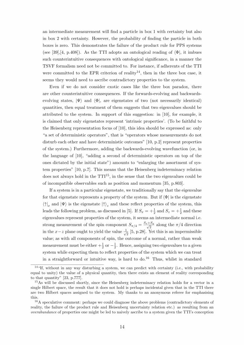
an intermediate measurement will find a particle in box 1 with certainty but also
in box 2 with certainty. However, the probability of finding the particle in both
boxes is zero. This demonstrates the failure of the product rule for PPS systems
(see [39],[4, p.408]). As the TTI adopts an ontological reading of 〈Φ|, it imbues
such counterintuitive consequences with ontological significance, in a manner the
TSVF formalism need not be committed to. For instance, if adherents of the TTI
were committed to the EPR criterion of reality14, then in the three box case, it
seems they would need to ascribe contradictory properties to the system.
Even if we do not consider exotic cases like the three box paradox, there
are other counterintuitive consequences. If the forwards-evolving and backwards-
evolving states, |Ψ〉 and 〈Φ|, are eigenstates of two (not necessarily identical)
quantities, then equal treatment of them suggests that two eigenvalues should be
attributed to the system. In support of this suggestion: in [10], for example, it
is claimed that only eigenstates represent ‘intrinsic properties’. (To be faithful to
the Heisenberg representation focus of [10], this idea should be expressed as: only
“a set of deterministic operators”, that is “operators whose measurements do not
disturb each other and have deterministic outcomes” [10, p.2] represent properties
of the system.) Furthermore, adding the backwards-evolving wavefunction (or, in
the language of [10], “adding a second of deterministic operators on top of the
ones dictated by the initial state”) amounts to “enlarging the assortment of sys-
tem properties” [10, p.7]. This means that the Heisenberg indeterminacy relation
does not always hold in the TTI15, in the sense that the two eigenvalues could be
of incompatible observables such as position and momentum [35, p.803].
If a system is in a particular eigenstate, we traditionally say that the eigenvalue
for that eigenstate represents a property of the system. But if 〈Φ| is the eigenstate
〈↑|x and |Ψ〉 is the eigenstate |↑〉z and these reflect properties of the system, this
leads the following problem, as discussed in [5]. If Sx = +12 and Sz = +1
2 and these
eigenvalues represent properties of the system, it seems an intermediate normal i.e.
strong measurement of the spin component Sπ/4 =Sx+Sy√
2along the π/4 direction
in the x−z plane ought to yield the value 1√2
[5, p.28]. Yet this is an impermissible
value; as with all components of spin, the outcome of a normal, rather than weak
measurement must be either +12 or−1
2 . Hence, assigning two eigenvalues to a given
system while expecting them to reflect properties of the system which we can treat
in a straightforward or intuitive way, is hard to do.16 Thus, whilst in standard
14“If, without in any way disturbing a system, we can predict with certainty (i.e., with probabilityequal to unity) the value of a physical quantity, then there exists an element of reality correspondingto that quantity” [23, p.777].
15As will be discussed shortly, since the Heisenberg indeterminacy relation holds for a vector in asingle Hilbert space, the result that it does not hold is perhaps incidental given that in the TTI thereare two Hilbert spaces assigned to the system. My thanks to an anonymous referee for emphasisingthis.
16A speculative comment: perhaps we could diagnose the above problems (contradictory elements ofreality, the failure of the product rule and Heisenberg uncertainty relation etc.) as resulting from anoverabundance of properties one might be led to naively ascribe to a system given the TTI’s conception
14
QM there is a problem about understanding indeterminate property possession
(for systems not in an eigenstate of the given quantity), the TTI faces difficulties
understanding property possession even for systems that are in eigenstates.
Proponents of the TTI might reject the traditional conception of properties cor-
responding to eigenvalues17 and provide an alternative criterion of reality: (one
such proposal is Vaidman’s ‘weak elements of reality’ [37]). This proposal is espe-
cially relevant since the traditionally impermissible 1√2
value just mentioned can
be ‘weakly’ measured on the system. Yet, if 〈Φ| only represents ‘weak’ properties,
we may doubt that its existence is really on a par with |Ψ〉.Given the difficulties assigning properties to a system described by 〈Φ| |Ψ〉, we
can conclude that at the very least more need to be said by proponents of the
TTI. However, such a project is motivated by an ontological commitment to 〈Φ|:and I will now argue that this commitment should be doubted.
As discussed in section 3.1.3, determinism requires that the state of the system
at any time (importantly, this includes the state of the system during the interme-
diate measurement time) is fixed by the ‘state’ (which in the TTI is the two-state
vector) at a single time in the course of the system’s history. Whilst at the time
of the intermediate measurement, we cannot access 〈Φ|, and thus we cannot at
that time predict with certainty the measurement outcome, adding 〈Φ| is what is
meant to determine the state of the system and thus, the measurement outcome.
However, generic pre- and postselection (and consequently the two-state vec-
tor) do not generally determine the outcome of the intermediate measurement.
They do so (under our governing assumption that the self-Hamiltonian is zero)
only in the special case where the intermediate observable is either identical to or
a function of the pre or postselection observables, as shown in Figure 4. If the
order of the measurements is reversed or the intermediate observable measured
is incompatible with the pre and postselection observables, the outcomes are not
determined. Unless the boundary conditions (PPS) are special, the outcome of
the intermediate measurement is still probabilistic (indeed otherwise the ABL rule
would be redundant as the probability of an outcome would be either 0 or 1).
This leads to two questions:
1. Since this theory is supposedly deterministic, what determines the interme-
diate result when 〈Φ| and |Ψ〉 do not?
2. In the case where 〈Φ| does determine the intermediate result, what deter-
mines 〈Φ|?According to the TTI, both questions have the same answer: there is an initial
state of the universe |Ψ〉HIS and a final state of the universe 〈Φ|DES as discussed
of quantum reality. Indeed, Price [31] questions whether “adding an additional wavefunction ‘comingfrom the future’ to standard QM and interpreting both wavefunctions in an ontic manner”... “fail[s] toexploit the ontological efficiency possible in a retrocausal model” [31, p.79] and suggests that “a singlebeable may be able to play both roles”.
17Indeed, a recent paper [9, p.142] suggests that this is the case.
15
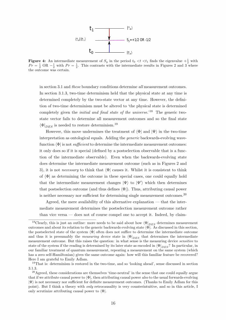
t0
t1
Sy=+1/2 OR -1/2
Figure 4: An intermediate measurement of Sy in the period t0 <t <t1 finds the eigenvalue + 12 with
Pr = 12 OR − 1
2 with Pr = 12 . This contrasts with the intermediate results in Figures 2 and 3 where
the outcome was certain.
in section 3.1 and these boundary conditions determine all measurement outcomes.
In section 3.1.3, two-time determinism held that the physical state at any time is
determined completely by the two-state vector at any time. However, the defini-
tion of two-time determinism must be altered to ‘the physical state is determined
completely given the initial and final state of the universe.’18 The generic two-
state vector fails to determine all measurement outcomes and so the final state
〈Φ|DES is needed to restore determinism.19
However, this move undermines the treatment of 〈Φ| and |Ψ〉 in the two-time
interpretation as ontological equals. Adding the generic backwards-evolving wave-
function 〈Φ| is not sufficient to determine the intermediate measurement outcomes:
it only does so if it is special (defined by a postselection observable that is a func-
tion of the intermediate observable). Even when the backwards-evolving state
does determine the intermediate measurement outcome (such as in Figures 2 and
3), it is not necessary to think that 〈Φ| causes it. Whilst it is consistent to think
of 〈Φ| as determining the outcome in these special cases, one could equally hold
that the intermediate measurement changes |Ψ〉 to |Ψ′〉 which then determines
that postselection outcome (and thus defines 〈Φ|). Thus, attributing causal power
is neither necessary nor sufficient for determining single measurement outcomes.20
Agreed, the mere availability of this alternative explanation — that the inter-
mediate measurement determines the postselection measurement outcome rather
than vice versa — does not of course compel one to accept it. Indeed, by claim-
18Clearly, this is just an outline: more needs to be said about how 〈Φ|DES determines measurementoutcomes and about its relation to the generic backwards evolving state 〈Φ|. As discussed in this section,the postselected state of the system 〈Φ| often does not suffice to determine the intermediate outcomeand thus it is presumably the measuring device state in 〈Φ|DES that determines the intermediatemeasurement outcome. But this raises the question: in what sense is the measuring device sensitive tostate of the system if the reading is determined by its later state as encoded in 〈Φ|DES? In particular, inour familiar treatment of quantum measurement, repeating a measurement on the same system (whichhas a zero self-Hamiltonian) gives the same outcome again: how will this familiar feature be recovered?Here I am grateful to Emily Adlam.
19That is: determinism is restored in the two-time, and so ‘looking ahead’, sense discussed in section3.1.3.
20Agreed, these considerations are themselves ‘time-neutral’ in the sense that one could equally arguethat if we attribute causal power to 〈Φ|, then attributing causal power also to the usual forwards-evolving|Ψ〉 is not necessary nor sufficient for definite measurement outcomes. (Thanks to Emily Adlam for thispoint). But I think a theory with only retrocausality is very counterintuitive, and so in this article, Ionly scrutinize attributing causal power to 〈Φ|.
16

ing that it is neither necessary nor sufficient to attribute causal power to 〈Φ| for
ensuring single measurement outcomes, I am not claiming that there is no project
in QM for which retrocausality may be important. But I am claiming that adding
a causally efficacious backwards-evolving state is not the ingredient that needs to
be added to quantum reality in order to solve the measurement problem.21
Hence, in order to ensure single measurement outcomes it is neither necessary
nor (in most cases) sufficient to attribute ‘causal power’ to 〈Φ| and thus there is
reason to doubt its existence. At the very least, it seems to have causal power
to a lesser degree than the forwards-evolving state. This is reminiscent of the
pilot-wave theory, where the wavefunction contributes to determining the motion
of — ‘kicks’ the corpuscles — but the corpuscles do not ‘kick’ back [13], [29, p.79],
[16, p.39]. Does the forwards-evolving wavefunction affect the backwards-evolving
wavefunction but not vice versa? If so, then this theory might be said to violate
the action-reaction principle in the same way that the pilot-wave theory has been
accused of doing [13].
Thus, I believe that, even by their own lights, Aharonov et al. should re-
ject the existence of 〈Φ| — or at least, its existence as on an equal footing with
|Ψ〉. Aharonov et al. are committed to ontological parsimony [9, p.143]; their
dissatisfaction with other interpretations such as the Everett and pilot-wave inter-
pretations stems from their “requiring additional entities” and hold that “entities
are not be multiplied beyond necessity” [2, p.2]. The postulated final state of
the universe 〈Φ|DES is vital to the success of TTI; it ensures that macroscopic
superpositions are not predicted and it determines measurement outcomes. The
generic backwards-evolving state 〈Φ| is not so industrious: and hence ontological
parsimony suggests one should not be committed to its existence.
6 A positive proposal
I have argued that the ontological reading of the backwards-evolving wavefunction
in TTI has many undesirable features. However 〈Φ| seems highly suggestive as it
arises from physical practice (postselection) and leads to novel phenomena (weak
values): thus, I would now like to end by endorsing an alternative interpretation.
Instead of Aharonov’s proposal, I favour Vaidman’s interpretation of 〈Φ| [38].22
If the backwards-evolving state of the measuring device is ‘up’ just in the
case that is what is later observed, then it is an encoding of our knowledge at a
later time. This epistemological interpretation is more modest; no causal power is
attributed to 〈Φ|. Further, 〈Φ| does not encode any properties of the system prior
21Nor is my argument an objection to Price’s argument [31]. Price’s argument looks at the conse-quences of having a time-symmetric ontology (namely that under certain assumptions, time-symmetryimplies retrocausality), whereas I am concerned with whether we should have a time-symmetric ontologyin the first place.
22For a full exposition of Vaidman’s views on the many worlds interpretation and TSVF, see [41].
17
to the postselection and so the difficulties around property possession and assigning
two eigenvalues disappear. Moreover, this epistemological interpretation requires
no assumptions about the final state of the universe. However, removing these
problems comes at a price — one can no longer claim to have an interpretation of
quantum mechanics.23 Yet, since I have argued that the TTI does not solve the
measurement problem, I believe this is a more natural reading of 〈Φ|.
6.1 〈Φ| and Everett
This epistemological reading of 〈Φ| fits naturally into the Everettian framework.
In the TTI’s strategy to solve the measurement problem, tracing over the en-
vironment in the two-time density matrix left one measurement outcome (‘up’).
However, this reduction was only effective (yielding an improper rather than a
proper mixture); the complete system (including the environment) is still in a
superposition after the measurement. In the Everettian picture, both branches of
the superposition still exist as distinct (emergent) worlds. However, 〈up| leads to
the effective reduction, pointing to one branch. Thus, as suggested by Vaidman
[38, p.593], the backwards-evolving state can be used to index which Everettian
world you were previously in. Whereas in the TTI, an unusual weak value would
be evidence for unusual final boundary conditions, in the Everettian picture it
would be evidence of being in a low amplitude branch.
Indeed, the idea of a final state of the universe that cannot be known about
(though it has to have a special form and contain records of all the measurements
ever made) and yet causally determines the present by propagating backwards
in time is, I think, no more plausible than positing a multiverse. Further, the
novel phenomena such as weak values that motivated the TVSF and TTI fit well
within the Everettian framework. As such, this proposal captures the desirable
features of the TTI: without the difficulties outlined in this paper. However, this
alternative proposal may not sit comfortably with adherents of the TTI; their
philosophical motivation was to find a time-symmetric quantum theory and the
Everettian branching structure is clearly asymmetric in time (see [45, ch.5]).
7 Conclusion
Whilst the TTI involves many interesting ideas, such as weak measurement, I
believe that these ideas do not currently amount to an interpretation of QM, since
— as I have argued — the two-time interpretation fails to solve the measurement
problem. Since the empirical probabilities were put in by hand to the postulated
final state of the universe without an underlying dynamical reason, this algorithm
23Recall that I argued in section 4 that specifying a particular outcome in accordance with ourexperience begs the question in the context of solving the measurement problem as it stipulates, ratherthan explains, single measurement outcomes.
18

was left unexplained (section 4). Further, few would count the theory as well-
formulated since the notion of measurement is primitive. In addition, I have
argued that it is neither necessary nor sufficient for ensuring single measurement
outcomes to attribute causal power to 〈Φ|. This militates against the existence
of 〈Φ|. So I have advocated rejecting the TTI and its ontological reading of 〈Φ|(section 5). However, Vaidman’s epistemological reading of 〈Φ| was seen to be
successful, particularly within the Everettian framework (section 6).
Acknowledgements
For their help and comments on previous versions, I would like to thank three
anonymous referees (especially for guidance to the burgeoning literature on the
TSVF and TTI). I am indebted to Jeremy Butterfield for his extensive comments
and to James Ladyman for his encouragement to work and publish on this topic.
This work was funded by the Arts and Humanities Research Council.
References
[1] Aharonov, Y., Bergmann, P. G. and Lebowitz, J.L. Phys. Rev. 134, B1410
(1964).
[2] Aharonov, Y. and Gruss, E. Two-time interpretation of quantum mechanics,
arXiv:quant-ph/0507269v1, (2005).
[3] Aharonov, Y. and Rohrlich, D. Quantum Paradoxes, Weinheim : Wiley-VCH,
(2005).
[4] Aharonov, Y. and Vaidman, L. The two-state vector formalism: An updated
review Lect. Notes Phys, 734, 399-447 (2008).
[5] Aharonov, Y., Popescu, S. and Tollaksen, J. A time-symmetric formulation
of quantum mechanics Physics Today, Volume 63, Issue 11, pp. 27-33 (2010).
[6] Aharonov, Y., Albert, D. and Vaidman, L. How the Result of a Measurement
of a Component of a Spin 1/2 Particle Can Turn Out to Be 100? Phys. Rev.
Lett. 60, 1351-1354 , (1988).
[7] Aharonov, Y., Cohen, E., Elitzur, A.C. Can a future choice affect a past
measurement? Ann. Phys. 355, 258-268, (2015).
[8] Aharonov, Y., Cohen, E., Elitzur, A.C. Foundations and applications of weak
quantum measurements Phys. Rev. A 89, 052105, (2014).
[9] Aharonov, Y., Cohen, E., Gruss, E., Landsberger, T. Measurement and Col-
lapse within the Two-State Vector Formalism Quantum Stud.: Math. Found.
1, 133-146, (2014).
[10] Aharonov, Y., Landsberger, T., Cohen, E., A nonlocal ontology underlying
the time-symmetric Heisenberg representation, arXiv:1510.03084v3, (2016).
19
[11] Aharonov, Y., Reznik, B., How macroscopic properties dictate microscopic
probabilities, Phys. Rev. A 65 052116, (2002).
[12] Albert, D. Quantum mechanics and experience, Cambridge, Mass; London:
Harvard University Press, (1994).
[13] Anandan, J. and Brown, H.R. On the Reality of Space-Time Geometry and
the Wavefunction, Found. Phys, Vol. 25, No. 2 (1995).
[14] Bell, J.S. Speakable and Unspeakable in Quantum Mechanics, 2nd. ed, Cam-
bridge: Cambridge University Press, (1987).
[15] Bell, J.S. Against ‘measurement’ in Speakable and Unspeakable in Quantum
Mechanics, 2nd. ed, Cambridge: Cambridge University Press, (1987).
[16] Bohm, D. and Hiley, B., The Undivided Universe: An Ontological Interpre-
tation of Quantum Theory, Routledge, (1993).
[17] Butterfield, J., Determinism and indeterminism, in the Routledge Ency-
clopaedia of Philosophy, (2005).
[18] Cohen, E., Aharonov, Y., Quantum to Classical Transitions via Weak Mea-
surements and Post-Selection To be published as a book chapter in ”Quan-
tum Structural Studies: Classical Emergence from the Quantum Level”, R.E.
Kastner, J. Jeknic-Dugic, G. Jaroszkiewicz (Eds.), World Scientific Publish-
ing Co. (2016). arXiv:1602.05083
[19] Danan, A., Farfurnik, D., Bar-Ad, S., Vaidman, L. Asking Photons Where
They Have Been PRL 111, 240402, (2013).
[20] Duck,I. M.,Stevenson, P. M., Sudarshan, E. C. G., The sense in which a
“weak measurement” of a spin-particle’s spin component yields a value 100
Phys. Rev. D, 40, 6, (1989).
[21] Earman, J., Determinism: what we have learned and what we still don’t know,
in Joseph K. Campbell (ed.), Freedom and Determinism. Cambridge Ma:
Bradford Book/MIT Press 21-46, (2004).
[22] Earman, J., The past hypothesis: not even false, Studies in History and Phi-
losophy of Science Part B: Studies in History and Philosophy of Modern
Physics, 37, 3, 399–430 (2006)
[23] Einstein, A., B. Podolsky, and N. Rosen, Can Quantum-Mechanical Descrip-
tion of Physical Reality Be Considered Complete?, Physical Review, 47: 777-
780, (1935).
[24] Fuchs, C. and Peres, A. Quantum Theory needs no ‘Interpretation’. Physics
Today, March pp.70-71. (2000).
[25] Gell-Mann, M. and Hartle, J. Time symmetry and asymmetry in quantum
mechanics and quantum cosmology in Physical Origins of Time Asymmetry,
ed by J. Halliwell, J. Perez-Mercader, and W. Zurek, Cambridge University
Press, Cambridge, (1994).
[26] Gruss, E. A Suggestion for a Teleological Interpretation of Quantum Mechan-
ics, arXiv:quant-ph/0006070, (2000).
20

[27] Hartle, J.B. and Hawking, S.W. The Wave Function of the Universe, Phys.
Rev. D 28, 2960-2975 (1983).
[28] Hawking, S.W. The Quantum State of the Universe, Nucl. Phys. B, 239, 257-
276, (1984).
[29] Holland, P., The Quantum Theory of Motion, CUP, (1993).
[30] Miller, D.J. Quantum mechanics as a consistency condition on initial and fi-
nal boundary conditions, Studies in History and Philosophy of Modern Physics
39, 767-781, (2008).
[31] Price, H. Does Time-Symmetry Imply Retrocausality? How the Quantum
World Says “Maybe” Studies in History and Philosophy of Modern Physics,
43, 75-83, (2012).
[32] Redhead, M. Incompleteness, Nonlocality, and Realism, Oxford : Clarendon
Press ; New York : Oxford University Press, (1987).
[33] Shimony, A. Events and Processes in the Quantum World in R. Penrose
and C. Isham, eds., Quantum Concepts in Space and Time (Oxford: Oxford
University Press), 182-203. Reprinted in Shimony 1993, 140-62. (1986)
[34] Tollaksen, J., Aharonov, Y., The Deterministic set of Operators, Quantum
Interference Phenomena, and Quantum Reality, Journal of Physics: Confer-
ence Series, Vol. 196, 1. (2009).
[35] Vaidman, L, The Two-State Vector Formalism in D. Greenberger, K.
Hentschel, F. Weinert, eds., Compendium of Quantum Physics: Concepts,
Experiments, History and Philosophy, (Springer) (2009).
[36] Vaidman, L. Emergence of Weak Values, in Quantum Interferometry, VCH
Publishers (1996), edited by F. De Martini (1996).
[37] Vaidman, L. Weak Measurement Elements of Reality Foundations of Physics,
Volume 26, Issue 7, pp 895-906 (1996).
[38] Vaidman, L. Time Symmetry and the Many-Worlds Interpretation, in ‘Many
Worlds? Everett, Quantum theory, and Reality’, (2010).
[39] L. Vaidman, Lorentz-invariant ‘elements of reality’ and the joint measurability
of commuting observables, Phys. Rev. Lett. 70, 3369, (1993)
[40] L. Vaidman, Past of a quantum particle, Phys. Rev. A, 87, 052104, (2013).
[41] L. Vaidman, Quantum Theory and Determinism, Quantum Stud.: Math.
Found. 1, 5-38, (2014). arXiv:1405.4222
[42] Wallace, D. Quantum Mechanics, Chpt. 1 in the Ashgate companion to Con-
temporary Philosophy of Physics, Aldershot: Ashgate, (2008).
[43] Wallace, D. Decoherence and its Role in the Modern Measurement Problem,
Philosophical Transactions of the Royal Society of London, A 370 (2012).
[44] Wallace, D. Gravity, entropy, and cosmology: In search of clarity, The British
Journal for the Philosophy of Science, 61, 513-540, (2010).
[45] Wallace, D. The Emergent Multiverse: Quantum Theory According to the
Everett Interpretation, OUP Oxford, (2014).
21
[46] Davies, P.C.W., Twamley, J., Time-symmetric cosmology and the opacity of
the future lightcone Class. Quant. Grav. 10, 931, (1993).
22


![Linguistic Copenhagen interpretation of quantum mechanics ......Linguistic Copenhagen interpretation of quantum mechanics: Quantum Language [Ver. 5] Shiro ISHIKAWA (ishikawa@math.keio.ac.jp)](https://img.pdfslide.net/doc/110x75/5ff4cf8b5ae30f5f7a653fc8/linguistic-copenhagen-interpretation-of-quantum-mechanics-linguistic-copenhagen.jpg)