Can we illuminate our cities and (still) see the stars?

S. Bará et. al/International Journal of Sustainable Lighting IJSL (2021) xx-xx

1

Can we illuminate our cities and (still) see the stars?

Salvador Bará1,*, Fabio Falchi1,2, Raul C. Lima3,4, Martin Pawley5

1 Departamento de Física Aplicada, Universidade de Santiago de Compostela, 15782

Santiago de Compostela, Galicia 2 Istituto di Scienza e Tecnologia dell’Inquinamento Luminoso (ISTIL), 36016

Thiene, Italy.

3 Escola Superior de Saúde do Politécnico do Porto, 4200-072 Porto, Portugal

4 Instituto de Astrofísica e Ciências do Espaço (IA), Universidade de Coimbra,

PT3040-004, Coimbra, Portugal

5 Agrupación Astronómica Coruñesa Ío, 15005 A Coruña, Galicia

Abstract

Could we enjoy starry skies in our cities again? Arguably yes. The actual number of visible stars will depend,

among other factors, on the spatial density of the overall city light emissions. In this paper it is shown that

reasonably dark skies could be achieved in urban settings, even at the center of large metropolitan areas, if the

light emissions are kept within admissible levels and direct glare from the light sources is avoided. These results

may support the adoption of science-informed, democratic public decisions on the use of light in our municipalities,

with the goal of recovering the possibility of contemplating the night sky everywhere in our planet.

Keywords: sustainable lighting, light pollution, sky brightness, radiometry, photometry.

1. Introduction

A common tenet of the dark skies movement is to try to preserve the dark areas still existing in the world,

avoiding their further deterioration. This position, often implemented through different figures of protection like

certified Starlight Tourist Destinations [1-2], IDA's International Dark Sky Places [3], and other astro-tourism

initiatives [4-8], not only intended for pristine dark sites, but also addressing urban parks and star observing spots

in polluted areas, has brought extremely significant benefits to the cause of the night and should no doubt be

further promoted. Notwithstanding that, a purely defensive, reactive stance seems to be nowadays insufficient for

ensuring the future of the dark nights in the planet. The persistent increase of radiance and illuminated surface [9]

progressively encroaches the dark areas, reducing their size and natural values [10-12]. The dark territory to defend

becomes progressively smaller and fragmentary, breaking in many cases the continuity of the nocturnal ecological

corridors [13].

A related ethical and political issue is whether or not we should collectively renounce to restoring the quality

of the night in areas already deteriorated, particularly in the most conspicuous ones, our urban nuclei. It is often

taken for granted that the night skies are irremediably lost there, due to the huge amount of light produced in our

urban agglomerations. Conventional wisdom considers the present level of emissions unavoidable. There is

however an ongoing trend to reassess the validity of some "old truths" regarding the required light levels in cities:

modern research fails once and again to find convincing reasons to support the actual recommendations for road

lighting [14], be it in the name of a purported traffic safety, fostering of compulsive consumption, or the even less

proven effect of increased photons densities when it comes to avoid some behaviors, see e.g. [15-20]. Recovering

the night sky in our metropolitan areas should therefore not be discarded a priori. The explicit position of this short

paper is that decidedly remediating deteriorated skies should be the option by default, and that this goal should not

be abandoned excepting where and when proven unfeasible.

*S. Bará, E-mail address: [email protected]


2

Assuming that a significant amount of light will be used anyway in populated areas, a natural question arises:

which is the maximum level of emissions compatible with ensuring a given darkness of the urban night sky?

Which are the compromises and balances? This work provides some general estimates of the order of magnitude

of the maximum allowable emissions, with the aim of contributing to the open discussion of this issue. Establishing

the "red-lines" [21] for the celestial nightscapes that we collectively desire for the nights of the places where we

live is a necessary pre-requisite for negotiating these goals against other legitimate social wishes.

2. Seeing the stars

Several well-known factors limit the ability of the human visual system to detect the faintest visible stars. Some

of them are directly related to the eye optics and the first steps of neural image processing that determine the

minimum luminance required to detect a beam of light, as well as the luminance contrast thresholds to identify the

presence of a celestial object against a lit background. The overall performance of our visual system results from

the interplay of the quantum efficiency of the retinal photoreceptors, the photon noise, the pre-processing of the

detected signals by the first post-receptor layers of the retina (horizontal, bipolar, amacrine, and ganglion cells)

and the subsequent cortical processing [22]. The fraction of incoming radiation entering the eye and reaching the

individual photoreceptors in the retina is itself dependent on the pupil size and spectral transmittance of the ocular

media of the observer (both age-related), as well as on the presence or not of residual uncorrected ametropia and

on the typical size of the ocular point-spread function associated to the physiological aberrations of the healthy

human eye [23-24]. Last but not least, the use or not of binocular vision, and the experience of the observer may

significantly influence their ability to detect the faintest stars.

For many practical applications all these factors can be summarized in a single number, namely the luminance

contrast threshold required to detect the presence of a stimulus of a given angular size against a more or less bright

background, under the prevailing observing conditions [25]. The concept of luminance contrast threshold is key

for assessing the possibility of detecting stars. Be it defined as a Weber fraction or as a Michelson contrast, the

existence of this threshold requires that, as the background luminance increases, the object luminance must also

increase –depending on the luminance adaptation state of the eye, and not necessarily in a linear way– to be in the

limit of detection. Any increase of the luminance of the background will then result in a limitation of our ability

to detect faint stars.

The natural sky background over which we see the stars is by no means absolutely dark in the optical region of

the spectrum, even in moonless nights during the astronomical night. Besides the unresolved stars of the Milky

Way, it has contributions from the galactic and extragalactic diffuse light, the light scattered by the zodiacal cloud

and, especially, the highly variable atmospheric airglow [26]. After entering the Earth's atmosphere part of this

light is scattered by molecules and aerosols, contributing that way to increase the visual background (or

foreground, perhaps a more appropriate denomination in this case). On the other hand, the direct radiance of the

sky objects propagated along the line of sight is attenuated by the atmosphere through the complementary

mechanisms of scattering out of the beam and absorption along the path, thus contributing to a further reduction

of the contrast of the stars. Everything else being equal, the natural sky is brighter at greater elevations above sea

level, and the number of visible stars shall decrease as the observers approach the sea baseline and/or look towards

larger zenith angles, as shown by Cinzano and Falchi [27]. All these factors can be quantified, for a given observing

site, time, and atmospheric conditions, by means of the Gaia-Hipparcos multi-band map of the natural night sky

brightness [26], and its associated GAMBONS web tool [28]. Needless to say, all of these background light sources

and attenuation effects are themselves an integral part of the natural sky we seek to preserve or recover, not an

effect to avoid or remediate.

Artificial light sources, in turn, add scattered photons and in some cases also direct ones to the observed scene,

further reducing the contrasts. It is not always fully realized that this artificial sky brightness is not generated "in

the sky" or in some particular layer of the atmosphere high above our heads, but it is a highly distributed

phenomenon due to the cumulative contributions of photons scattered across the air column along our line of

vision, starting at the very first millimeter in front of our eyes. Depending on the location of the sources, their

angular and spectral emission patterns, and the aerosol types and concentration profiles, the maximum contribution

to the total amount of atmospheric scattered radiation entering our eyes will be generated at some definite altitude

above ground, but all path length elements have definitely their share, from millimeter one, so to speak.

Additionally, the radiance directly entering our eyes from directions in the periphery of the visual field (e.g. from

unshielded streetlights) is strongly scattered in the intra-ocular media [29-30], giving rise to an additional large

number of photons superimposed onto the photoreceptor receptive fields that further reduce the contrast, a


3

phenomenon usually termed glare. Finally, an additional extra-atmospheric source of background artificial light

is the diffuse radiance of the satellite and space debris cloud [31].

All of the above put together, it is possible to formulate reasonably comprehensive and accurate models for

predicting the limiting magnitudes of the stars that can be seen by humans under a variety of observing conditions.

Detailed formulations can be found in the classical works by Shaeffer [32-34], which are the key references in this

field, and in other related publications [35-37].

A proxy commonly used in the light pollution research community for reporting the visual quality of the night

sky is the total sky brightness in the Johnson V band, specified in magV/arcsec2. The use of the Johnson V band

[38-39] is partly motivated by historical reasons and should probably be revised in the near future. From a visual

point of view the Johnson V band turns out to be suboptimal: the sky luminance in the photopic [40], scotopic

[41], or mesopic [42-43] human vision bands should be routinely reported instead, whereas for large-scale,

worldwide light pollution instrument-based measurement and reporting campaigns the scientific photometric

system defined for the standard RGB bands [44], such as those used in science-, industry-, and consumer-grade

digital cameras [45], seems to be the-most efficient choice. For the purposes of this work, the quality of the urban

night sky will be characterized with two metrics commonly used in this field: the total zenith sky brightness in

Johnson magV/arcsec2, and the photopic artificial zenith luminance, in cd/m2. The latter will be natively evaluated

in the CIE photopic 𝑉(𝜆) band, i.e. not transformed from the Johnson V radiance (for the issues associated with

this transformation see [46-47]). The use of these well-known metrics is intended to facilitate a first discussion of

the issue of the restoration of urban skies. More comprehensive metrics, including all-sky and near-horizon

average brightnesses [48-50] should be taken into account in future works for a full formulation of the desired

features of the urban nightscapes.

3 City emissions and artificial sky brightness

3.1. Model and parameters

To answer the question that motivates this paper it is convenient to analyze a simplified situation that

nevertheless captures the basic physics of the problem. There is no fundamental difficulty for computing more

accurate results, tailored for any actual urban configuration one may wish, and no doubt these calculations should

be performed in any particular city when it comes to adopting science-informed public decisions on lighting.

However, such a level of detail does not seem to be necessary for giving an order-of-magnitude answer to the issue

addressed here.

Let us then consider a plausible scenario: an observer located within small urban park of radius, say, 𝑅0~200

m, embedded in the center of a wide metropolitan area of arbitrary radius 𝑅. To avoid short-distance scattering

effects as well as the glare due to the direct radiance of the streetlights entering the eyes of the observer, let us

assume that the park is reasonably free from annoying artificial light sources. This does not preclude the existence

of light sources to illuminate the pedestrian paths, as long as their light –including the one reflected off the ground–

is neither redirected in appreciable amounts towards the sky nor towards the observer eyes, being perhaps blocked

by the tree canopy.

Let us further assume that the city light emissions are spatially homogeneous in average, that is, that the amount

of artificial light emitted per unit of city surface, Φ𝐿, measured in lm·m–2 (or, equivalently, in Mlm·km–2) is

reasonably constant across the metropolitan area. Under these assumptions, and with some additional information,

the zenith brightness at the observer location can be easily calculated from the spectral power density of the city

lights by using the extremely simplified model described in the Appendix, eq. (A12). Different approaches can be

used to compute the required point-spread functions (PSF) that describe the propagation of light from the street

lamps to the observer [51-57]. For illustrating the examples below we used the Illumina v2.0 spectral PSFs

calculated by Simoneau et al (2021), available in the excellent paper [58]. These PSFs are given in [58] as a

function of the distance to the source for different wavelengths, specific luminaire angular emission patterns with

different fractions of light directly emitted to the upper hemisphere (ULOR), obstacle heights (h), and aerosol

optical depths (AOD), keeping constant other parameters as the luminaire pole height, street form factor, spectral

reflectance of the terrain, and the atmospheric conditions other than AOD, e. g., the aerosol composition, albedo

and scattering phase functions. Previous versions of Illumina PSFs (v1.0) had been successfully used to compute

the artificial sky brightness in other settings, see, e.g. [59-60].

The Johnson V photometric system adopted here is the one described in [26], using the classical Bessell

passband and a Vega-based magnitude scale in which magVega=+0.03, which corresponds to a zero-point reference


4

radiance 𝐵𝑟𝑒𝑓 = 143.1682 W·m–2·sr–1. The brightness of the natural sky in the Johnson V band is an important

parameter for interpreting the measured sky brightness, which is the sum of the natural and artificial components.

The natural brightness of the zenith night sky adopted here is 𝑚𝑁 = 22.0 magV/arcsec2, a value conventionally

used for this kind of studies [10]. Note that the zenith natural brightness is actually highly variable in time, since

it depends on the patch of the sky located around the zenith region at each moment, as well as on the intensity of

the airglow and the overall state of the atmosphere. The interested readers may want to use slightly different values

for their locations, times, and atmospheric conditions, information freely available in the GAMBONS website

[28]. The GAMBONS tool has also been used here to determine a reasonable value for the visual luminance of

the natural sky, set to 200 cd/m2. This reference natural luminance, determined natively in the CIE photopic

visual band by using the Gaia-Hipparcos map of the brightness of the natural sky [26], is consistent with the values

determined in an indirect way, namely by performing appropriate conversions from the Johnson V band radiance

[46-47], and it should be recommended as a default value instead of the less realistic 174 cd/m2 frequently quoted

in the literature.

3.2. Results

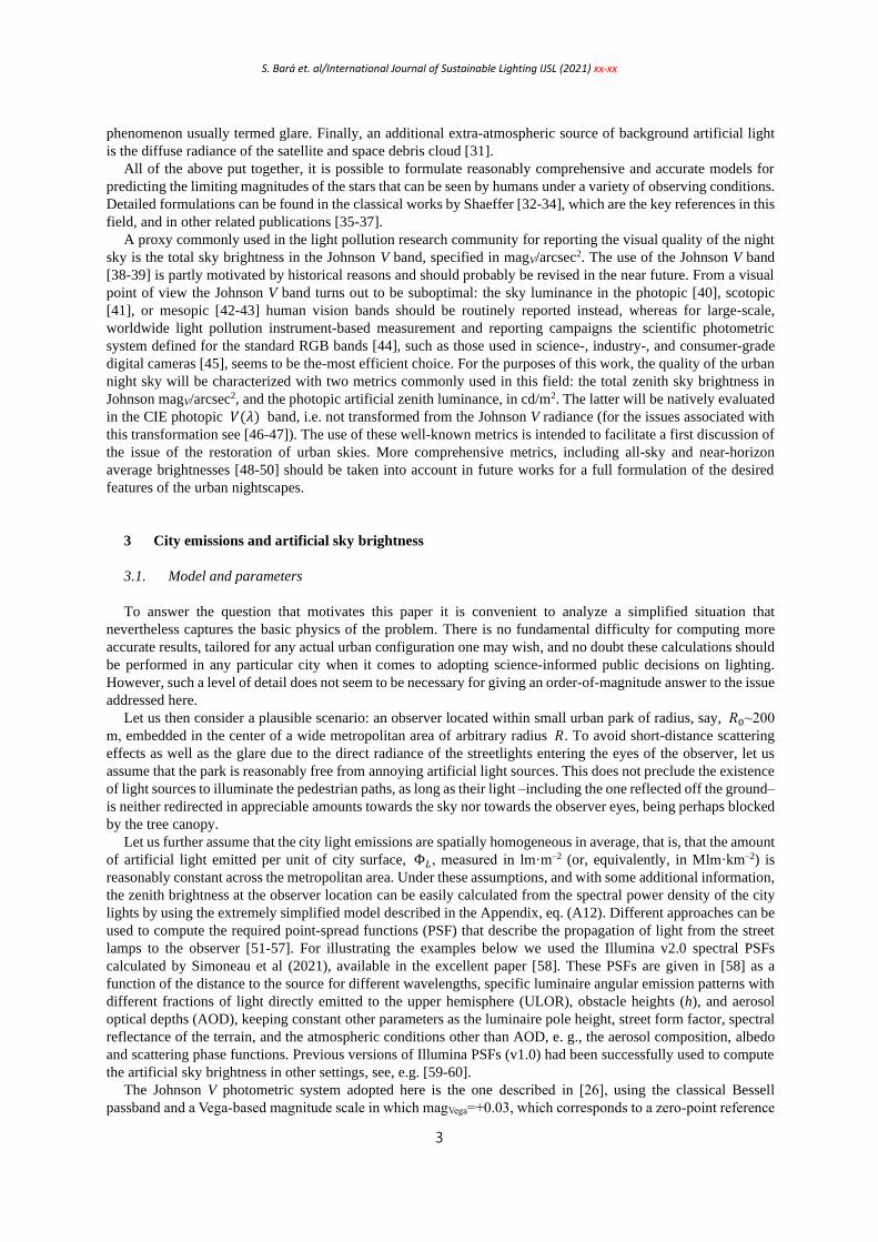
Figure 1 displays the total (natural + artificial) zenith brightness of the sky in the Johnson V band, expressed in

magV/arcsec2 (Fig 1a) as well as the artificial component of the photopic zenith luminance given in mcd/m2 =10–3

cd/m2 (Fig 1b), for an urban area whose light sources are entirely composed by 3000 K CCT LED, typical obstacle

height 9 m, ULOR=5% and an atmosphere with an aerosol optical depth (AOD) of 0.2, corresponding to a visibility

of about 26 km. The values associated to the different lines shown in the legend (1, 2, 3, 5, 10), correspond to

different levels of city light emissions spatial densities, Φ𝐿, expressed in lm·m–2. These values can be converted

to average illuminances at street level, 𝐸, in lx, by using the formula 𝐸 = 𝜂Φ𝐿 𝜖⁄ where 𝜂 = 1 − ULOR is the

fraction of radiant flux emitted towards the lower hemisphere, and 𝜖 is the fraction of the city territory actually

illuminated, i.e. excluding roofs and other zones where no direct light arrives. Given the relatively low ULOR

value of the sources considered in this figure, the average street illuminance is approximately equal to ~Φ𝐿 𝜖⁄ to

within a 5%, such that if the outdoor spaces directly lit occupy, say, only one half of the city surface, 𝜖 = 0.5,

then the average street illuminance (in lx) compatible with attaining a given level of sky darkness (in magV/arcsec2)

will be twice the number indicated in the legend.

Fig. 1. Brightness of the zenith sky for different amounts of emitted artificial light (legend in lm·m–2), versus city size. Left: total brightness

(including the natural component) in the Johnson V band, in magV/arcsec2. Right: artificial component luminance in mcd/m2. See text for

details.

According to this figure and under the assumed conditions, a city of radius 4 km, with 𝜖 = 0.5 could in

principle attain zenith skies slightly darker than 20.0 magV/arcsec2 if its outdoor spaces are lit with an average

illuminance not surpassing 6 lx (blue dash-dotted line of emissions 3 lm·m–2). Achieving 21.0 magV/arcsec2 is

definitely possible if the overall emissions do not surpass 1 lm·m–2. Keep in mind that these results are contingent

on the assumption of an isolated city, such that no other urban area adds polluting photons to the sky of the observer.

As the size of the city increases, the emission densities compatible with a given darkness of the sky tend to decrease,

due to the additional light contributions from the city rings of increasing area 𝑟 d𝑟 located at progressively larger


5

distances from the observer. Note, however, that the contributions from larger 𝑟 are exponentially attenuated by

the atmosphere, so the total brightness increases at a progressively smaller rate with city size.

The actual brightness of the sky is of course highly variable along the night and throughout the seasons,

depending on the evolution of the artificial light emissions and the continuously changing atmospheric conditions.

Cities with different urban structures are expected to experience different levels of sky brightness, due to the

particular types of angular emission patterns and spectra of their light sources, the different kind of obstacles and

the specific spectral reflectance of their surfaces. To get some insights about the variability associated to some of

these factors, the following figures display the total sky brightness in the Johnson V band and the artificial

component of the zenith sky luminance for several combinations of them.

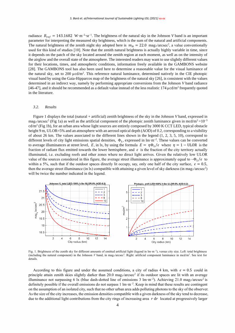
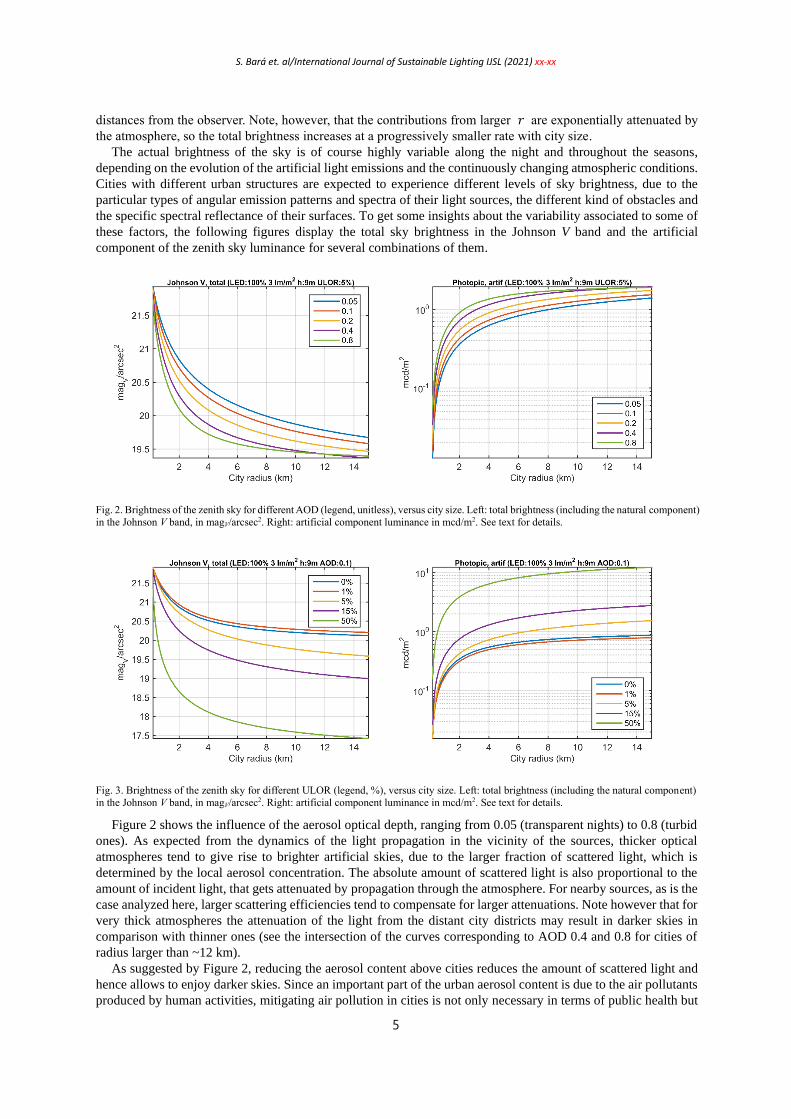
Fig. 2. Brightness of the zenith sky for different AOD (legend, unitless), versus city size. Left: total brightness (including the natural component)

in the Johnson V band, in magV/arcsec2. Right: artificial component luminance in mcd/m2. See text for details.

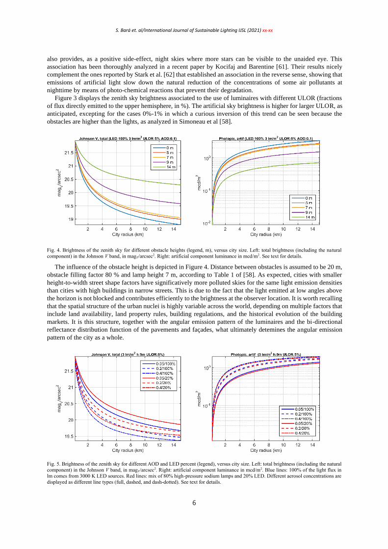
Fig. 3. Brightness of the zenith sky for different ULOR (legend, %), versus city size. Left: total brightness (including the natural component)

in the Johnson V band, in magV/arcsec2. Right: artificial component luminance in mcd/m2. See text for details.

Figure 2 shows the influence of the aerosol optical depth, ranging from 0.05 (transparent nights) to 0.8 (turbid

ones). As expected from the dynamics of the light propagation in the vicinity of the sources, thicker optical

atmospheres tend to give rise to brighter artificial skies, due to the larger fraction of scattered light, which is

determined by the local aerosol concentration. The absolute amount of scattered light is also proportional to the

amount of incident light, that gets attenuated by propagation through the atmosphere. For nearby sources, as is the

case analyzed here, larger scattering efficiencies tend to compensate for larger attenuations. Note however that for

very thick atmospheres the attenuation of the light from the distant city districts may result in darker skies in

comparison with thinner ones (see the intersection of the curves corresponding to AOD 0.4 and 0.8 for cities of

radius larger than ~12 km).

As suggested by Figure 2, reducing the aerosol content above cities reduces the amount of scattered light and

hence allows to enjoy darker skies. Since an important part of the urban aerosol content is due to the air pollutants

produced by human activities, mitigating air pollution in cities is not only necessary in terms of public health but


6

also provides, as a positive side-effect, night skies where more stars can be visible to the unaided eye. This

association has been thoroughly analyzed in a recent paper by Kocifaj and Barentine [61]. Their results nicely

complement the ones reported by Stark et al. [62] that established an association in the reverse sense, showing that

emissions of artificial light slow down the natural reduction of the concentrations of some air pollutants at

nighttime by means of photo-chemical reactions that prevent their degradation.

Figure 3 displays the zenith sky brightness associated to the use of luminaires with different ULOR (fractions

of flux directly emitted to the upper hemisphere, in %). The artificial sky brightness is higher for larger ULOR, as

anticipated, excepting for the cases 0%-1% in which a curious inversion of this trend can be seen because the

obstacles are higher than the lights, as analyzed in Simoneau et al [58].

Fig. 4. Brightness of the zenith sky for different obstacle heights (legend, m), versus city size. Left: total brightness (including the natural

component) in the Johnson V band, in magV/arcsec2. Right: artificial component luminance in mcd/m2. See text for details.

The influence of the obstacle height is depicted in Figure 4. Distance between obstacles is assumed to be 20 m,

obstacle filling factor 80 % and lamp height 7 m, according to Table 1 of [58]. As expected, cities with smaller

height-to-width street shape factors have significatively more polluted skies for the same light emission densities

than cities with high buildings in narrow streets. This is due to the fact that the light emitted at low angles above

the horizon is not blocked and contributes efficiently to the brightness at the observer location. It is worth recalling

that the spatial structure of the urban nuclei is highly variable across the world, depending on multiple factors that

include land availability, land property rules, building regulations, and the historical evolution of the building

markets. It is this structure, together with the angular emission pattern of the luminaires and the bi-directional

reflectance distribution function of the pavements and façades, what ultimately detemines the angular emission

pattern of the city as a whole.

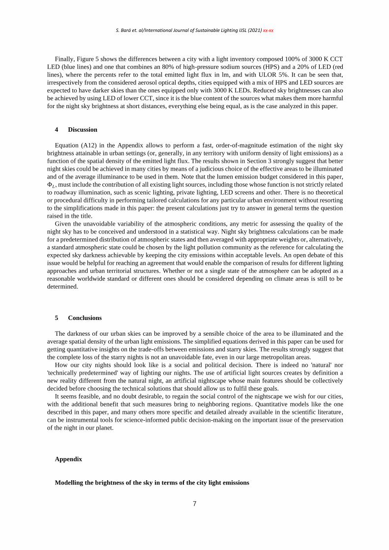
Fig. 5. Brightness of the zenith sky for different AOD and LED percent (legend), versus city size. Left: total brightness (including the natural

component) in the Johnson V band, in magV/arcsec2. Right: artificial component luminance in mcd/m2. Blue lines: 100% of the light flux in

lm comes from 3000 K LED sources. Red lines: mix of 80% high-pressure sodium lamps and 20% LED. Different aerosol concentrations are

displayed as different line types (full, dashed, and dash-dotted). See text for details.


7

Finally, Figure 5 shows the differences between a city with a light inventory composed 100% of 3000 K CCT

LED (blue lines) and one that combines an 80% of high-pressure sodium sources (HPS) and a 20% of LED (red

lines), where the percents refer to the total emitted light flux in lm, and with ULOR 5%. It can be seen that,

irrespectively from the considered aerosol optical depths, cities equipped with a mix of HPS and LED sources are

expected to have darker skies than the ones equipped only with 3000 K LEDs. Reduced sky brightnesses can also

be achieved by using LED of lower CCT, since it is the blue content of the sources what makes them more harmful

for the night sky brightness at short distances, everything else being equal, as is the case analyzed in this paper.

4 Discussion

Equation (A12) in the Appendix allows to perform a fast, order-of-magnitude estimation of the night sky

brightness attainable in urban settings (or, generally, in any territory with uniform density of light emissions) as a

function of the spatial density of the emitted light flux. The results shown in Section 3 strongly suggest that better

night skies could be achieved in many cities by means of a judicious choice of the effective areas to be illuminated

and of the average illuminance to be used in them. Note that the lumen emission budget considered in this paper,

Φ𝐿, must include the contribution of all existing light sources, including those whose function is not strictly related

to roadway illumination, such as scenic lighting, private lighting, LED screens and other. There is no theoretical

or procedural difficulty in performing tailored calculations for any particular urban environment without resorting

to the simplifications made in this paper: the present calculations just try to answer in general terms the question

raised in the title.

Given the unavoidable variability of the atmospheric conditions, any metric for assessing the quality of the

night sky has to be conceived and understood in a statistical way. Night sky brightness calculations can be made

for a predetermined distribution of atmospheric states and then averaged with appropriate weights or, alternatively,

a standard atmospheric state could be chosen by the light pollution community as the reference for calculating the

expected sky darkness achievable by keeping the city emissions within acceptable levels. An open debate of this

issue would be helpful for reaching an agreement that would enable the comparison of results for different lighting

approaches and urban territorial structures. Whether or not a single state of the atmosphere can be adopted as a

reasonable worldwide standard or different ones should be considered depending on climate areas is still to be

determined.

5 Conclusions

The darkness of our urban skies can be improved by a sensible choice of the area to be illuminated and the

average spatial density of the urban light emissions. The simplified equations derived in this paper can be used for

getting quantitative insights on the trade-offs between emissions and starry skies. The results strongly suggest that

the complete loss of the starry nights is not an unavoidable fate, even in our large metropolitan areas.

How our city nights should look like is a social and political decision. There is indeed no 'natural' nor

'technically predetermined' way of lighting our nights. The use of artificial light sources creates by definition a

new reality different from the natural night, an artificial nightscape whose main features should be collectively

decided before choosing the technical solutions that should allow us to fulfil these goals.

It seems feasible, and no doubt desirable, to regain the social control of the nightscape we wish for our cities,

with the additional benefit that such measures bring to neighboring regions. Quantitative models like the one

described in this paper, and many others more specific and detailed already available in the scientific literature,

can be instrumental tools for science-informed public decision-making on the important issue of the preservation

of the night in our planet.

Appendix

Modelling the brightness of the sky in terms of the city light emissions


8

In this paper the term "brightness", 𝐵, is meant to denote the radiance (expressed either in W·m–2·sr–1 or in

photon·s–1·m–2·sr–1, depending on the choice of the radiometric system) contained within the spectral sensitivity

band 𝑆(𝜆) of the detector. 𝐵 is calculated by integrating the sky spectral radiance 𝐿(𝜆), given in units W·m–

2·sr–1·nm–1 or photon·s–1·m–2·sr–1·nm–1, within the 𝑆(𝜆) band, as

𝐵 = ∫ 𝑆(𝜆)𝐿(𝜆)d𝜆

∞

0

(A1)

A similar definition can be applied to any sky quality indicator linearly dependent on the spectral radiance at

the observer location, including, but not limited to, the zenith radiance, the average hemispheric radiance, the

horizontal illuminance, or the average radiance within some angular strip above the horizon [46-48]. The

formulation developed below applies equally to any of these indicators, and hence 𝐵 may be understood as

representing any of them; for the particular purpose of this paper, however, we will identify 𝐵 with the zenith

sky brightness.

The spectral bands 𝑆(𝜆) analyzed here are the Johnson-Cousins V [26] and the CIE visual photopic sensitivity

band 𝑉(𝜆) [40]. Their associated photometric systems are defined, by historical reasons, in terms of energies

instead of photon numbers, even if the actual interactions of the radiation with the detectors take place on a photon

basis. When working with human visual bands in the photopic, scotopic or mesopic adaptation ranges the in-band

radiance, expressed in energy units, can be converted into SI luminous units of cd·m–2 by multiplying it by the

corresponding luminous efficacy coefficients, namely 𝐾𝑚 = 683 lm·W–1 for photopically adapted eyes, 𝐾′𝑚 =1700 lm·W–1 for scotopically adapted ones, and intermediate values for mesopic adaptation [43].

The spectral radiance 𝐿(𝐫0, 𝜆) at the observer position 𝐫0 can be expressed as a weighted linear combination

of the spectral radiant flux emitted by the surrounding light sources. If Φ(𝐫, 𝜆)d2𝐫 is the spectral radiant flux

(W·nm–1) emitted by the sources contained within the elementary area d2𝐫 (m2), such that Φ(𝐫, 𝜆) is the spectral

radiant flux emitted per unit of territory surface (W·m–2·nm–1), the linear nature of this problem allows to write

[63-64]:

𝐿(𝐫0, 𝜆) = ∫ Φ(𝐫, 𝜆)Ψ(𝐫, 𝐫0, 𝜆)d2𝐫

𝐴

(A2)

where Ψ(𝐫, 𝐫0, 𝜆) is the point-spread function (m–2·sr–1) that accounts for the atmospheric propagation and for

the angular emission pattern of the sources, assumed to be spectrally and angularly factorable [63], and for the

effects related to the terrain (ground and façade reflections, obstacle blocking, etc). The integral is extended to 𝐴,

the relevant territory containing the sources that contribute to the radiance at the observer location. This formal

model allows us to use directly the PSF functions proposed by Simoneau et al [58].

As a side note, recall that alternative expressions similar to Eq. (A2) could be written for computing 𝐿(𝐫0, 𝜆)

in terms of other inputs. For instance, Φ(𝐫, 𝜆)d2𝐫 could be taken to mean the spectral radiant flux leaving a given

patch d2𝐫 of the territory, not the spectral flux leaving the luminaires, in which case the ground and façade

reflections and the obstacle blocking effects would be included in the values of Φ rather than in Ψ (that would

then basically describe the atmospheric propagation effects). The input Φ(𝐫, 𝜆) to Eq. (A2) could also be another

practical radiometric quantity, for instance the spectral radiance 𝐿(𝐫, 𝜆) of the terrain at d2𝐫 (W·m–2·sr–1·nm–1),

as described in [63], in which case calibrated radiance satellite images could be used as inputs and the PSF will

have units m–2.

In what follows and for the purposes of the examples presented in this paper we assume that the point-spread

function (PSF) Ψ is shift-invariant, that is, spatially homogenous, such that its value depends on the relative

position of the source with respect to the observer but not on the absolute positions of them

Ψ(𝐫, 𝐫0, 𝜆) = Ψ(𝐫 − 𝐫0, 𝜆) (A3)

and we further impose rotational symmetry such that

Ψ(𝐫, 𝐫0, 𝜆) = Ψ(𝑟, 𝜆) (A4)

where 𝑟 = ‖𝐫 − 𝐫0‖ is the source-to-observer distance .


9

For the purposes of this paper it will be also assumed that the observer is located in an urban park or star

observing spot reasonably free from nearby and direct light emission sources within a small zone of radius 𝑅0,

but surrounded by a wide city or metropolitan area of radius 𝑅. For a preliminary order-of-magnitude assessment

we will further assume that the urban emissions have a uniform spatial density, i.e. that they can be considered

homogeneous across the territory when aggregated within each surface integral element d2𝐫, so that the spectral

flux density does not depend on the position within the city, and hence Φ(𝐫, 𝜆) = Φ(𝜆). Under these conditions

the radiance at the observer location can be expressed as

𝐿(𝐫0, 𝜆) ≡ 𝐿(𝜆; 𝑅) = Φ(𝜆) ∫ ∫ Ψ(𝑟, 𝜆) 𝑟 d𝑟 d𝜑

𝑅

𝑅0

2𝜋

0

= 2𝜋 Φ(𝜆) ∫ Ψ(𝑟, 𝜆) 𝑟 d𝑟

𝑅

𝑅0

(A5)

Once 𝐿(𝜆; 𝑅) is known, the zenith sky brightness in the photometric observation band 𝑆(𝜆), i.e., the in-

band integrated radiance 𝐵(𝑅), dependent on the size of the surrounding light-emitting territory, is:

𝐵(𝑅) = ∫ 𝑆(𝜆)𝐿(𝜆; 𝑅)d𝜆

∞

0

= 2𝜋 ∫ ∫ 𝑆(𝜆)Φ(𝜆)Ψ(𝑟, 𝜆) 𝑟 d𝑟 d𝜆

∞

0

𝑅

𝑅0

(A6)

and the corresponding value of the anthropogenic brightness of the sky in magnitudes per square arcsecond,

𝑚𝑎𝑟𝑡𝑖𝑓, is

𝑚𝑎𝑟𝑡𝑖𝑓 = −2.5 log10

𝐵(𝑅)

𝐵𝑟𝑒𝑓

(A7)

where 𝐵𝑟𝑒𝑓 is the zero-point of the magnitude scale, that can be arbitrarily chosen but shall be explicitly specified,

associated via Eq. (A1) to a reference spectral radiance 𝐿𝑟𝑒𝑓(𝜆). Two usual choices to define the zero-point of

the magnitude scales in astronomy are the spectral irradiance of the star Vega (a Lyr) and the absolute AB

irradiance proposed by Oke [65], after expressing them as the radiances of a patch of the sky of size 1 arcsec2 that

would produce these irradiances at the entrance of the observing instrument [46].

To calculate the observed sky magnitude the contribution of the natural sky brightness shall be added to the

numerator of the log argument in Eq. (A7). If the natural sky brightness in the chosen photometric band is assumed

to be 𝑚𝑁, expressed in mag/arcsec2, then the in-band radiance of the natural sky is 𝐵𝑁 = 𝐵𝑟𝑒𝑓 10−0.4×𝑚𝑁, and

the total brightness in magnitudes per square arcsecond measured by the observer, 𝑚, will be

𝑚 = −2.5 log10

𝐵𝑁 + 𝐵(𝑅)

𝐵𝑟𝑒𝑓

= −2.5 log10 [ 10−0.4×𝑚𝑁 +𝐵(𝑅)

𝐵𝑟𝑒𝑓

] (A8)

Finally, from the above equations one gets:

𝑚 = −2.5 log10 [ 10−0.4×𝑚𝑁 +2𝜋

𝐵𝑟𝑒𝑓

∫ ∫ 𝑆(𝜆)Φ(𝜆)Ψ(𝑟, 𝜆) 𝑟 d𝑟 d𝜆

∞

0

𝑅

𝑅0

] (A9)

In summary, Eq. (A9) provides 𝑚, the total brightness of the sky in mag/arcsec2 in the 𝑆(𝜆) band, expressed in

a magnitude scale with a zero-point defined by the radiance 𝐵𝑟𝑒𝑓 , measured by an observer in the center of an

unlit park of radius 𝑅0 surrounded by a territory of radius 𝑅 whose luminaires emit a spatially averaged

homogeneous spectral flux Φ(𝜆) , with the atmospheric conditions, terrain features, and luminaire angular

emission patterns accounted for in the shift-invariant and rotationally symmetric PSF Ψ(𝑟, 𝜆) , when the

magnitude of the natural sky is 𝑚𝑁.

The spectral radiant flux emitted by the city by unit of urban surface, Φ(𝜆), can be rewritten in terms of the

spatial density of emitted light, Φ𝐿 , in lm·m–2 (equivalent to Mlm·km–2) by recalling that the photopic

luminous flux Φ𝐿 associated to a spectral radiant flux Φ(𝜆) is:


10

Φ𝐿 = 𝐾𝑚 ∫ 𝑉(𝜆)Φ(𝜆)d𝜆

∞

0

(A10)

where 𝑉(𝜆) is the CIE photopic spectral sensitivity function and 𝐾𝑚 = 683 lm·W–1. Denoting by Φ̂(𝜆) the

normalized radiant flux producing exactly one lumen, we have Φ(𝜆) = Φ𝐿 Φ̂(𝜆), where

Φ̂(𝜆) =Φ(𝜆)

𝐾𝑚 ∫ 𝑉(𝜆)Φ(𝜆)d𝜆∞

0

(A11)

has units W·lm–1·nm–1. Note that the W·lm–1 units stem from the 𝐾𝑚 factor in the denominator, so for

the purpose of calculating Φ̂(𝜆) it is possible to use a Φ(𝜆) dataset in arbitrary linear units per nm (they

cancel out in Eq. (A11)), which is a convenient option when the shapes of the lamp spectra are known but not

their calibrated radiometric flux. With this notation Eq. (A9) becomes

𝑚 = −2.5 log10 [ 10−0.4×𝑚𝑁 +2𝜋Φ𝐿

𝐵𝑟𝑒𝑓

∫ ∫ 𝑆(𝜆)Φ̂(𝜆)Ψ(𝑟, 𝜆) 𝑟 d𝑟 d𝜆

∞

0

𝑅

𝑅0

] (A12)

Finally, if the fraction of radiant flux emitted towards the lower hemisphere is 𝜂 = 1 − ULOR, and the fraction

of the territory surface actually illuminated is 𝜖 (encompassing all illuminated city locations, i.e. excluding roofs

and other zones where no direct light actually arrives), the average ground illuminance 𝐸, in lx, is given by 𝐸 = 𝜂Φ𝐿 𝜖⁄ .

Acknowledgments

This work was supported in part by Xunta de Galicia, grant ED431B 2020/29.

References

[1] Marín, C. & Jafari, J. (2008). StarLight: A Common Heritage; StarLight Initiative La Palma Biosphere Reserve, Instituto De Astrofísica De Canarias, Government of The Canary Islands, Spanish Ministry of The Environment, UNESCO-MaB: Canary Islands, Spain.

[2] Starlight Foundation. (2015). List of Starlight Tourist Destinations. https://fundacionstarlight.org/en/section/list-of-starlight-tourist-destinations/293.html (last accessed May 15, 2021)

[3] International Dark-Sky Association. (2021). International Dark Sky Places conservation program https://www.darksky.org/our-work/conservation/idsp/ (last accesssed July 7, 2021)

[4] Blundell, E., Schaffer, V., & Moyle, B. D. (2020). Tourism Recreation Research, 45(4), 549-556, doi: 10.1080/02508281.2020.1782084

[5] Kanianska, R., Škvareninová, J., & Kaniansky, S. (2020). Landscape Potential and Light Pollution as Key Factors for Astrotourism Development: A Case Study of a Slovak Upland Region. Land, 9, 374. doi:10.3390/land9100374

[6] Mitchell, D., & Gallaway, T. (2019). Dark sky tourism: economic impacts on the Colorado Plateau Economy, USA. Tourism Review, 74(4), 930-942. doi: 10.1108/TR-10-2018-0146

[7] Paül, V., Trillo-Santamaría, J. M., Haslam-Mckenzie, F. (2019). The invention of a mountain tourism destination: An exploration of Trevinca-A Veiga (Galicia, Spain). Tourist Studies, 19(3), 313-335. doi:10.1177/1468797619833364

[8] Weaver, D. (2011). Celestial ecotourism: new horizons in nature-based tourism, Journal of Ecotourism, 10(1), 38-45, doi: 10.1080/14724040903576116

[9] Kyba, C. C. M., Kuester, T., Sánchez de Miguel, A., Baugh, K., Jechow, A., Hölker, F., Bennie, J., Elvidge, C. D., Gaston, K. J., & Guanter, L. (2017). Artificially lit surface of Earth at night increasing in radiance and extent. Sci. Adv. 3, e1701528. doi: 10.1126/sciadv.1701528

[10] Falchi, F., Cinzano, P., Duriscoe, D., Kyba, C. C. M., Elvidge, C. D., Baugh, K., Portnov, B. A., Rybnikova, N. A., & Furgoni, R. (2016). The new world atlas of artificial night sky brightness. Sci. Adv. 2, e1600377, doi: 10.1126/sciadv.1600377


11

[11] Gaston, K. J., Duffy, J. P., & Bennie, J. (2015), Quantifying the erosion of natural darkness in the global protected area system. Conservation Biology, 29, 1132-1141. doi:10.1111/cobi.12462

[12] Davies, T.W., Duffy, J.P., Bennie, J., & Gaston, K.J. (2016). Stemming the Tide of Light Pollution Encroaching into Marine Protected Areas. Conservation Letters 29(3),164–171. doi: 10.1111/conl.12191

[13] Ditmer, M. A., Stoner, D. C., & Carter, N. H. (2021). Estimating the loss and fragmentation of dark environments in mammal ranges from light pollution. Biological Conservation, 257, 109135. doi: 10.1016/j.biocon.2021.109135.

[14] Fotios, S., Gibbons, R. (2018). Road lighting research for drivers and pedestrians: The basis of luminance and illuminance recommendations. Lighting Research & Technology, 50(1), 154-186. doi:10.1177/1477153517739055

[15] Marchant, P. (2005). Shining a light on evidence-based policy: street lighting and crime. Criminal Justice Matters, 62(1), 18-45. di: 10.1080/09627250508553093

[16] Marchant, P. (2010). What is the contribution of street lighting to keeping us safe? An investigation into a policy. Radic. Stat., 102, 32–42. http://www.radstats.org.uk/no102/Marchant102.pdf.

[17] Marchant P. (2017). Why Lighting Claims Might Well Be Wrong. International Journal of Sustainable Lighting, 19, 69-74. doi: 10.26607/ijsl.v19i1.71

[18] Marchant P. (2019) Do brighter, whiter street lights improve road safety? Significance, 16(5), 8-9. doi: 10.1111/j.1740-9713.2019.01313.x

[19] Marchant P., Hale, J. D., Sadler, J. P. J (2020). Does changing to brighter road lighting improve roadsafety? Multilevel longitudinal analysis of road traffic collision frequency during the relighting of a UK city. Epidemiol Community Health, 74,467–472. doi:10.1136/jech-2019-212208

[20] Marchant P. (2020). Bad Science: Comments on the paper ‘Quantifying the impact of road lighting on road safety — A New Zealand Study’ by Jackett & Frith (2013). World Transport Policy and Practice, 26(2), 10-20.

[21] Bará, S., Falchi, F., Lima, R. C., Pawley, M. (2021) Keeping light pollution at bay: a red-lines, target values, top-down approach. Environmental Challenges (in press)

[22] Frisby, J. P., & Stone, J. V. (2010). Seeing: The Computational Approach to Biological Vision, 2nd. Ed., MIT Press.

[23] Navarro, R., & Losada, M. A. (1997). Shape of stars and optical quality of the human eye. Journal of the Optical Society of America A, 14, 353-359.

[24] Thibos, L.N., Hong, X., Bradley, A., & Cheng, X. (2002). Statistical variation of aberration structure and image quality in a normal population of healthy eyes. Journal of the Optical Society of America A, 19(12), 2329-2348.

[25] Blackwell, H. R. (1946). Contrast Thresholds of the Human Eye. Journal of the Optical Society of America, 36(11), 624-643. doi: 10.1364/JOSA.36.000624

[26] Masana, E., Carrasco, J. M., Bará, S., & Ribas, S.J. (2021). A multi-band map of the natural night sky brightness including Gaia and Hipparcos integrated starlight. Monthly Notices of the Royal Astronomical Society, 501, 5443–5456. doi 10.1093/mnras/staa4005

[27] Cinzano, P., & Falchi, F. (2020). Toward an atlas of the number of visible stars. Journal of Quantitative Spectroscopy & Radiative Transfer, 253, 107059. doi: 10.1016/j.jqsrt.2020.107059

[28] GAMBONS, The GAia Map of the Brightness Of Natural Sky. https://gambons.fqa.ub.edu/ (Last accessed July 7, 2021)

[29] van den Berg, T. J. T. P., Franssen, L., & Coppens, J. E. (2010). Ocular Media Clarity and Straylight. In Darlene A. Dartt (ed), Encyclopedia of the Eye, Vol 3. Oxford:Academic Press; pp. 173-183.

[30] van den Berg, T. J. T. P., Franssen, L., Kruijt, B., & Coppens, J. E. (2013). History of ocular straylight measurement: A review. Z. Med. Phys., 23, 6–20. doi: 10.1016/j.zemedi.2012.10.009

[31] Kocifaj, M., Kundracik, F., Barentine, J. C., Bará, S. (2021). The proliferation of space objects is a rapidly increasing source of artificial night sky brightness. Monthly Notices of the Royal Astronomical Society Letters, 504, L40–L44. doi:10.1093/mnrasl/slab030

[32] Schaefer, B.E. (1990). Telescopic limiting magnitudes, Publications of the Astronomical Society of the Pacific, 102, 212-229.

[33] Schaefer, B.E. (1991). Glare and Celestial Visibility, Publications of the Astronomical Society of the Pacific, 103, 645-660.

[34] Schaefer, B.E. (1993). Astronomy and the Limits of Vision. Vistas in Astronomy, 36, 311- 361. doi:10.1016/0083-6656(93)90113-X

[35] Upgren, A. R. (1991). Night-sky brightness from the visibility of stars near the horizon. Publications of the Astronomical Society of the Pacific, 103, 1292-1295.

[36] Cinzano, P., Falchi, F., Elvidge, C. D. (2001). Naked-eye star visibility and limiting magnitude mapped from DMSP-OLS satellite data. Mon. Not. R. Astron. Soc., 323, 34–46

[37] Crumey, A. (2014). Human contrast threshold and astronomical visibility. Mon. Not. R. Astron. Soc., 442, 2600–2619. doi:10.1093/mnras/stu992

[38] Bessell, M.S. (1990). UBVRI passbands. Publications of the Astronomical Society of the Pacific, 102, 1181-1199.

[39] Bessell, M., Murphy, S. (2012). Spectrophotometric Libraries, Revised Photonic Passbands, and Zero Points for UBVRI, Hipparcos, and Tycho Photometry. Pub Astr Soc Pac, 124, 140–157.

[40] CIE, Commision Internationale de l'Éclairage. (1990). CIE 1988 2° SpectralLuminous Efficiency Function for Photopic Vision. CIE 86:1990. Vienna: Bureau Central de la CIE.


12

[41] CIE, Commission Internationale de l’Éclairage (1951). Proceedings Vol. 1, Sec 4; Vol 3, p. 37. Paris: Bureau Central de la CIE.

[42] CIE, Commission Internationale de l’Éclairage. (2010). Recommended system for mesopic photometry based on visual performance. CIE 191:2010.

[43] Maksimainen, M., Kurkela, M., Bhusal, P., & Hyyppä, H. (2019). Calculation of Mesopic Luminance Using per Pixel S/P Ratios Measured with Digital Imaging, LEUKOS, 15(4), 309-317. doi: 10.1080/15502724.2018.1557526

[44] Cardiel, N., Zamorano, J., Bará, S., et al. (2021). Synthetic RGB photometry of bright stars: definition of the standard photometric system and UCM library of spectrophotometric spectra. Monthly Notices of the Royal Astronomical Society, 504(3), 3730-3748. doi: 10.1093/mnras/stab997

[45] Hänel, A., Posch, T., Ribas, S. J., et al. (2018). Measuring night sky brightness: methods and challenges. Journal of Quantitative Spectroscopy & Radiative Transfer, 205, 278–290. doi:10.1016/j.jqsrt.2017.09.008

[46] Bará, S., Aubé, M., Barentine, J., & Zamorano, J. (2020). Magnitude to luminance conversions and visual brightness of the night sky. Monthly Notices of the Royal Astronomical Society, 493, 2429–2437. doi: 10.1093/mnras/staa323

[47] Fryc, I., Bará, S., Aubé, M., Barentine, J. C. & Zamorano, J. (2021). On the Relation between the Astronomical and Visual Photometric Systems in Specifying the Brightness of the Night Sky for Mesopically Adapted Observers, LEUKOS, doi:10.1080/15502724.2021.1921593

[48] Duriscoe, D. M. (2016). Photometric indicators of visual night sky quality derived from all-sky brightness maps. Journal of Quantitative Spectroscopy & Radiative Transfer, 181, 33–45. doi: 10.1016/j.jqsrt.2016.02.022

[49] Duriscoe, D. M., Anderson, S. J., Luginbuhl, C. B., & Baugh, K. E. (2018). A simplified model of all-sky artificial sky glow derived from VIIRS Day/Night band data. Journal of Quantitative Spectroscopy & Radiative Transfer, 214, 133–145. doi: 10.1016/j.jqsrt.2018.04.028

[50] Falchi, F., & Bará, S. (2021). Computing light pollution indicators for environmental assessment. Nat Sci. e10019. doi: 10.1002/ntls.10019

[51] Garstang, R. H. (1989). Night-sky brightness at observatories and sites. PASP 101, 306. doi:10.1086/132436 [52] Cinzano, P., & Falchi, F. (2012).The propagation of light pollution in the atmosphere. Monthly Notices of

the Royal Astronomical Society 427(4), 3337–3357. doi: 10.1111/j.1365-2966.2012.21884.x [53] Aubé, M., & Simoneau, A. (2018). New features to the night sky radiance model illumina: Hyperspectral

support, improved obstacles and cloud reflection. Journal of Quantitative Spectroscopy and Radiative Transfer, 211, 25–34. doi: 10.1016/j.jqsrt.2018.02.033

[54] Kocifaj, M. (2007). Light-pollution model for cloudy and cloudless night skies with ground-based light sources. Appl Opt 46(15), 3013. doi: 10.1364/AO.46.003013

[55] Kocifaj, M. (2018). Multiple scattering contribution to the diffuse light of a night sky: A model which embraces all orders of scattering. Journal of Quantitative Spectroscopy and Radiative Transfer, 206, 260–72. doi: 10.1016/j.jqsrt.2017.11.020

[56] Bará, S., Rigueiro, I., & Lima, R. C. (2019). Monitoring transition: Expected night sky brightness trends in different photometric bands. Journal of Quantitative Spectroscopy and Radiative Transfer, 239, 106644. doi: 10.1016/j.jqsrt.2019.106644

[57] Aubé, M., Simoneau, A., Muñoz-Tuñón, C., Díaz-Castro, J., & Serra-Ricart, M. (2020). Restoring the night sky darkness at Observatorio del Teide: First application of the model Illumina version 2. Monthly Notices of the Royal Astronomical Society, 497(3), 2501–2516. doi: 10.1093/mnras/staa2113

[58] Simoneau, A., Aubé, M., Leblanc, J., Boucher, R., Roby, J., & Lacharité, F. (2021). Point spread functions for mapping artificial night sky luminance over large territories, Monthly Notices of the Royal Astronomical Society, 504(1), 951–963. doi: 10.1093/mnras/stab681

[59] Linares, H., Masana, E., Ribas, S. J., Garcia-Gil, M., Figueras, F., & Aubé, M. (2018). Modelling the night sky brightness and light pollution sources of Montsec protected area, Journal of Quantitative Spectroscopy and Radiative Transfer 217, 178-188. doi: 10.1016/j.jqsrt.2018.05.037

[60] Linares, H., Masana, E., Ribas, S. J., Aubé, M., Simoneau, A., & Bará, S. 2020. Night sky brightness simulation over Montsec protected area. Journal of Quantitative Spectroscopy and Radiative Transfer, 249, 106990. doi: 10.1016/j.jqsrt.2020.106990.

[61] Kocifaj, M., & Barentine, J. C. (2021). Air pollution mitigation can reduce the brightness of the night sky in and near cities. Sci Rep, 11, 14622. doi:10.1038/s41598-021-94241-1

[62] Stark, H., Brown, S. S., Wong, K. W., Stutz, J., Elvidge, C. D., Pollack, I. B., Ryerson, T. B., Dube, W. P., Wagner, N. L., & Parrish, D. D. (2011). City lights and urban air. Nature Geoscience 4, 730-731.

[63] Bará, S., & Lima, R. C. (2018). Photons without borders: quantifying light pollution transfer between territories, International Journal of Sustainable Lighting 20(2), 51-61. doi:10.26607/ijsl.v20i2.87

[64] Falchi, F., & Bará, S. (2020). A linear systems approach to protect the night sky: implications for current and future regulations. R.Soc. Open Sci., 7,201501. doi: 10.1098/rsos.201501

[65] Oke, J. B. (1974). Absolute spectral energy distributions for white dwarfs. The Astrophysical Journal Suppl. Series 236(27), 21-35.

Documents

Can we illuminate our cities and (still) see the stars?