Canal Investment, 1815-1860 · CANAL INVESTMENT, 1815-1860 TABLE 1 Development of a Sample Construction-Expenditure Profile, The Pennsylvania and Ohio Canal, 1835—1840 (dollar …

This PDF is a selection from an out-of-print volume from the NationalBureau of Economic Research

Volume Title: Trends in the American Economy in the Nineteenth Century

Volume Author/Editor: The Conference on Research in Income and Wealth

Volume Publisher: Princeton University Press

Volume ISBN: 0-870-14180-5

Volume URL: http://www.nber.org/books/unkn60-1

Publication Date: 1960

Chapter Title: Canal Investment, 1815-1860

Chapter Author: H. Jerome Cranmer

Chapter URL: http://www.nber.org/chapters/c2489

Chapter pages in book: (p. 547 - 570)

Canal Investment, i8iç—i86o

H. JEROME CRANMERDREW UNIVERSITY AND BANKERS TRUST COMPANY

IN THE United States, more than 4,000 miles of canals were builtbetween 1815 and 1860 at a cost of nearly $200 million. The presentpaper describes my attempt to develop a method of estimating annualexpenditures for particular canals, which are then combined to yieldregional and national totals and the relative investment of governmentand private enterprise. I also touch on the economic significance of thestatistical findings.

Method of EstimationFailure to keep adequate records, the destruction or loss of many

records, refusal to adhere to homogeneous categories in the analysis ofexpenditures, and the use of the annual reports to obscure rather thanclarify the fiscal operations of a company all have produced gaps in theprimary sources. My study is based largely upon published materialswhich include reports of internal improvement commissions and stateauditors, annual reports and other documents of private companies,contemporary surveys of internal improvements such as Armroyd,Mitchell, Tanner, and Poor; Purdy's survey in the 1880 census, thevaluable tables in Whitford's History of the Canal System of the Stateof New York, and many monographs on particular canals or canalsystems. The estimates, therefore, must be considered as only prelimi-nary. More definitive estimates must await meticulous examination ofmanuscript sources, such as the records of individual companies.1

Canals were classified according to the availability of informationabout them. The first category contained projects about which allnecessary information was available: total cost, annual expenditures,construction put in place but not paid for, and dimensions of the canal—mileage, lockage, area of prism, and so forth. In these happy cases itwas necessary only to assemble the annual expenditures, adjust themfor construction put in place but not paid for, and aggregate. Thiscategory accounted for $154 million, or some 79 per cent, of totalcanal investment.

The second category consisted of projects for which only partialexpenditure information was available. Dimensions, total cost, orperhaps total expenditures to a particular date were known but not

1 See Appendix A for a list of sources.

547

INVESTMENT

annual expenditure figures. This category provided about $33 million,or 17 per cent, of total canal investment. Here it was necessary todevise some means of apportioning total cost over the period of con-struction in order to get the desired annual estimates. For this purposea typical pattern of annual expenditures was developed from a sampleprovided by twenty-four canals in the first category.

The third category consisted of canals for which virtually no costswere known. Dimensions, as well as years of construction, were usuallyavailable however. For such projects it was necessary to develop a wayof estimating total cost which then could be distributed over the years ofconstruction by means of the typical pattern mentioned above, whichwas done by a multiple regression analysis based on a sample of forty-four canals provided by the first and second categories. This categoryaccounted for less than $6 million, or less than 3 per cent, of canalinvestment.

The fourth category consisted of a miscellany of canals about whichonly the most fragmentary information was available. Two factorswere essential: mileage and years of construction. When either wasmissing the canal could not be included in the estimates. Fortunatelythe category was small, amounting to less than $2 million of total canalinvestment.

The typical pattern for annual canal investment was developed by anaveraging process applied to the experience of a sample of twenty-fourcanals for which annual expenditure figures were available.2 Severalpreliminary operations were required.

1. The annual expenditure figures for each canal had to be adjustedto take account of construction put in place but for which contractorshad not been paid at the end of the fiscal year. Usually state boards ofinternal improvement and private canal companies withheld a percent-age from each voucher as a performance bond against the contractor.Moreover, vouchers for work completed might be in process of beingapproved or paid and thus not appear in expenditures for the fiscal yearin which the work was accomplished. A further adjustment was neces-sary to convert fiscal years into calendar years.

2. To be able to present both total expenditures and years of con-struction in comparable magnitudes, they had to be converted intopercentages. Adjusted annual expenditures were converted into annualpercentages of total cost, and calendar years of construction intoannual percentages of the total number of years of construction.

3. The next step was the computation of "C" coefficients—the ratioof the annual percentages of total cost to the annual percentages of totalyears of construction (Table 1).

2 See Appendix B for a list of these canals.

548

CANAL INVESTMENT, 1815-1860

TABLE 1Development of a Sample Construction-Expenditure Profile, The

Pennsylvania and Ohio Canal, 1835—1840(dollar figures in thousands)

Year

ConstructionExpenditures

AdjustedPercentage of

Total Cost

Percentage ofConstruction

PeriodC

Coefficient

183518361837183818391840

$ 32.1207.5264.1308.1277.3

46.1

2.8%18.323.227.124.4

4.1

16.7%16.716.716.716.716.7

0.171.101.391.621.460.25

$1,135.2 100.0% 100.0% 6.00

Source: Annual Reports of the Pennsylvania and Ohio Canal Co., 1836—1841.

CHART 1

Construction Expenditure Profile, Pennsylvania and Ohio Canal, 1835—1840

C2.00

1.75

1.50

1.25

1.00

.75

50

25

0•0

Source: Table 1.

549

10 20 30 40 50 60 70 80 90 100Per cent of construction period

IN VESTMENT

4. The coefficients were then plotted for each canal as in Chart 1,which provided a profile of its expenditure pattern.

Where canal expenditures were proportionately distributed over theperiod of construction, for example, 10 per cent of the cost incurred in10 per cent of the time, or 50 per cent of the cost in 50 per cent of thetime, the C coefficient is 1.00 throughout and the profile a horizontalline. However, as with the Pennsylvania and Ohio (Mahoning) CanalCompany, used as an illustration in Chart 1, annual expenditures wereby no means in proportion to period of construction. Rather the typicalpattern was for a small beginning, a crescendo to a peak about themiddle of the period, followed by a gradual decrescendo to the com-pletion of the canal.

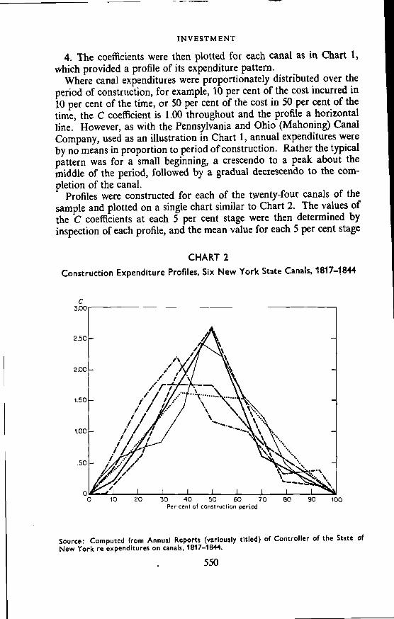
Profiles were constructed for each of the twenty-four canals of thesample and plotted on a single chart similar to Chart 2. The values ofthe C coefficients at each 5 per cent stage were then determined byinspection of each profile, and the mean value for each 5 per cent stage

CHART 2

Construction Expenditure Profiles, Six New York State Canals, 1817—1844

100

Source: Computed from Annual Reports (variously titled) of Controller of the State ofNew York re expenditures on canals, 1817—1844.

550

0 10 20 30 40 70 60 90Per cent of construction period

60


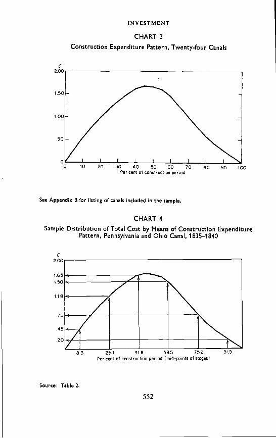
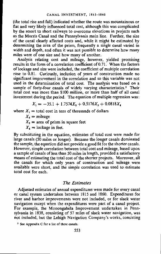
was computed. The result was a curve of means representing the averageexpenditure profile of the twenty-four canals. To smooth this curve, andparticularly to round off a fairly sharp peak at the 50 per cent stage, afive-term moving average was applied. The resulting curve, shown inChart 3, was taken as the typical pattern of canal construction expendi-ture, which provided a means of distributing the total cost of a particularcanal over the period of construction, as illustrated in Chart 4 and

TABLE 2Sample Distribution of Total Cost by Means of Construction Expenditure Pattern,

The Pennsylvania and Ohio Canal, 1835—1840(dollar figures in millions)

Year

Percentage ofConstruction

Period CoefficientPercentage of

Total CostAnnual

Esii'naiedExpenditures

Actual

1835 16.7% 0.45 7.8 $ 89 $ 32.!1836 16.7 1.18 20.6 234 207.51837 16.7 1.65 28.8 327 264.11838 16.7 1.50 26.2 297 308.11839 16.7 0.75 13.1 149 277.31840 16.7 0.20 3.4 39 46.1

100.2 99.9 1,135 1,135.2

Source: Chart 4 and Table 1.

Table 2. In this way estimates of annual expenditure were developedfrom total cost figures.

The second major problem encountered in estimating annual canalinvestment was posed by canals for which no total cost figures could befound. Fortunately, descriptive information was available for most ofthese. The most important item was, of course, the length of the canal.Other variables—the kind of terrain traversed by the canal, the size ofthe canal, the years in which the canal was building—also seemedsignificant. Total mileage figures were available for nearly all of theprojects. However, they were coniplicated'by such considerations aswhether or not the total mileage included "feeders" (canals for bringingwater to the main line), as for the Delaware and Raritan Canal and theUnion Canal of Pennsylvania. Total mileage figures were furthercomplicated where the canal consisted of slack water navigation, aswith the Lehigh Navigation Company; or where total mileage includedrailway or turnpike extensions, as with the Delaware and Hudson or theearly James River and Kanawha canals. It was generally impossible tofind detailed information about the terrain traversed by a canal—whether sand, clay, rock, marsh, or whatever. The amount of lockage

551

C2.00

1.50

1.00

.50

0

IN VESTMENT

CHART 3

Construction Expenditure Pattern, Twenty-four Canals

See Appendix B for listing of canals included in the sample.

Source: Table 2.

CHART 4

552

0 10 20 30 40 50 60 70 80 90 100Per cent of construction pertod

Sample Distribution of Total Cost byPattern, Pennsylvania and

Means of Construction ExpenditureOhio Canal, 1835—1840

C

2.00

1.65

1.50

1,18

.75

.45

.20

8.3 25.1 41.8 58.5 75.2 91.9

Per cent of construction period (mid-points of stages)


(the total rise and fall) indicated whether the route was mountainous orflat and very likely influenced total cost, although this was complicatedby the resort to short railways to overcome elevations in projects suchas the Morris Canal and the Pennsylvania main line. Further, the sizeof the canal clearly affected costs and, while it might be estimated bydetermining the area of the prism, frequently a single canal varied inwidth and depth, and often it was not possible to determine how manymiles were of one size and how many of another.

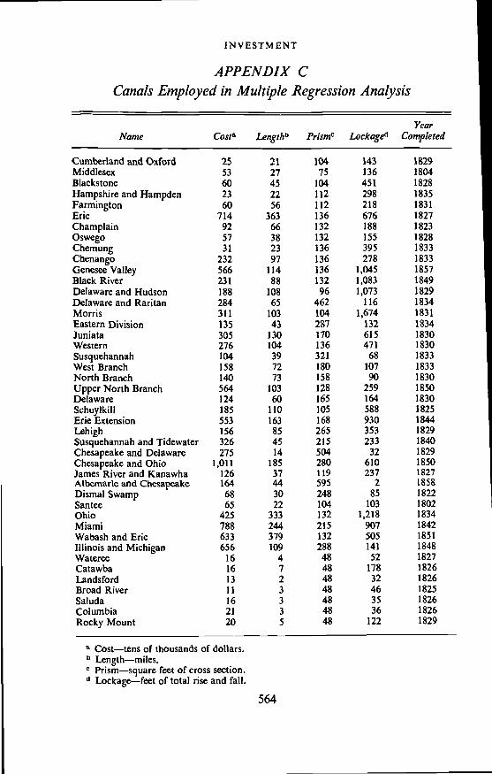
Analysis relating cost and mileage, however, yielded promisingresults in the form of a correlation coefficient of 0.71. When the factorsof lockage and size were included, the coefficient of multiple correlationrose to 0.81. Curiously, inclusion of years of construction made nosignificant improvement in the correlation and so this variable was notused in the determination of total cost. The analysis was based on asample of forty-four canals of widely varying characteristics.3 Theirtotal cost was more than $100 million, or more than half of all canalinvestment during the period. The equation of multiple regression was:

= —35.1 + l.7574X2 + 0.5176X3 + 0.0818X4where X1 = total cost in tens of thousands of dollars

A'2 = mileageA'3 = area of prism in square feetA'4 = lockage in feet.

By substituting in the equation, estimates of total cost were made forlarge canals (50 miles or longer). Because the longer canals dominatedthe sample, the equation did not provide a good fit for the shorter canals.However, simple correlation between total cost and mileage, based upona sample of canals of less than 50 miles in length, provided a satisfactorymeans of estimating the total cost of the shorter projects. Moreover, allthe canals for which only years of construction and mileage wereavailable were short, and the simple correlation was used tO. estimatetotal cost for each.

The EstimatesAdjusted estimates of annual expenditures were made for every canal

or canal system undertaken between 1815 and 1860. Expenditures forriver and harbor improvements were not included, or for slack waternavigation except when the expenditures were part of a canal project.For example, the Monongahela Improvement undertaken in Penn-sylvania in 1838, consisting of 57 miles of slack water navigation, wasnot included, but the Lehigh Navigation Company's works, consisting

See Appendix C for a list of these canals.

553

INVESTMENT

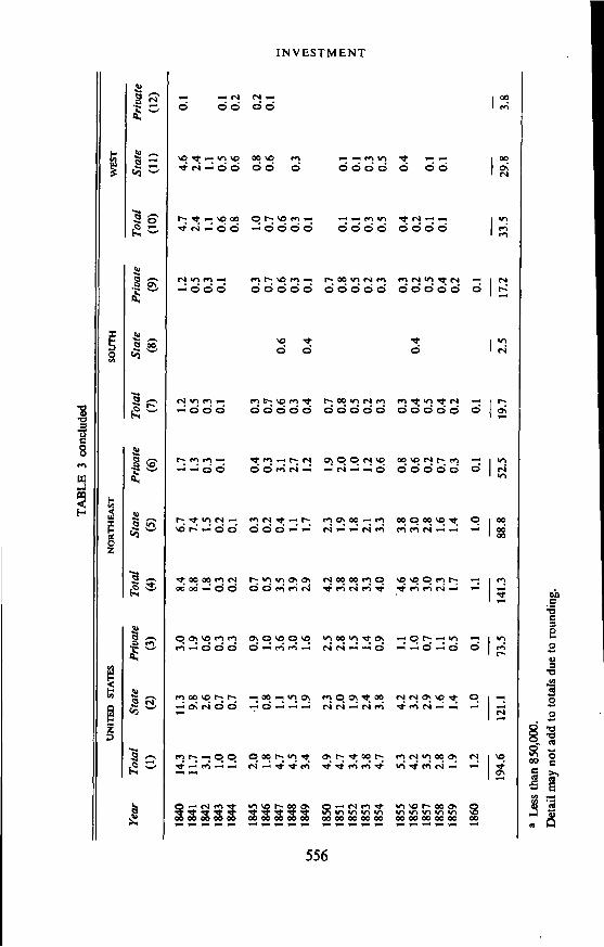
of 36 miles of canal and 12 miles of slack water navigation was, sinceexpenditures for the canal were indistinguishable from total expetidi-tures. The estimates were then aggregated by region and by agency ofenterprise within each region. The regional estimates were then aggre-gated to provide estimates of annual investment in canals for theentire United States, together with estimates for state and private enter-prise. The estimates appear in Table 3.

The data indicate three major cycles in canal investment over theperiod. From less than $50,000 in 1815, the first cycle cumulates throughthe twenties reaching a peak around 1829 and declining to a trough inthe thirties. By 1831, $50 million had been spent, and most of theprojects had been completed or were nearing completion. New canalswere being projected, and construction expenditures continued moder-ately high through the early thirties but not at the level reached earlier.

If profitability and life span be the test, the canals undertaken duringthis first wave were by far the most successful. This is particularly trueof the private canals. Led by the Delaware and Raritan, the list includesthe Delaware and Hudson, the Chesapeake and Delaware, the Lehighand the Schuylkill navigations, and the Morris Canal. The same cannotbe said of all private projects, however. The Farmington, the. Hamp-shire and Hampden, the Union, and others enjoyed a far less happy fateand soon were abandoned. The state projects undertaken during thefirst wave also compare favorably to the projects of the later periods.

The second cycle began in 1836; the expansion phase continued to the1840 peak and was followed by a precipitate drop to a trough in 1844.From more than $14 million in 1840, canal investment fell to less than$1 million in 1843 and again in 1844. Thus, while 1840 had the greatestvolume of canal investment of the entire period (twice the earlier peakand nearly three times the subsequent peak), within four years invest-ment had fallen to the lowest, level since 1819. During this nine-yearcycle some $70 million were invested in canal construction.

The second wave was distinguished from the earlier and later cyclesby a greater degree of public investment and of building in the West.Public investment constituted less than 60 per cent of total investmentin cycles one and three; in the second cycle it grew to almost 70 percent. And western investment, which did not reach 10 per cent of totalcanal investment in cycles one or three, was over 30 per cent in cycle two.The greater amplitude of the second cycle probably is attributable tothese two characteristics.

The third cycle began with an upturn in 1845, increased gradually toa mild peak in 1855, and then declined, once again gradually, to its endin 1860. This cycle was by far the mildest of the three in terms ofamplitude of fluctuations. With its termination came the end of sig-nificant canal investment in the United States.

554

TAB

LE 3

Ann

ual I

nves

tmen

t in

Can

als b

y R

egio

n an

d by

Age

ncy

of E

nter

pris

e, 1

815—

1860

(mill

ions

of d

olla

rs)

UN

ITED

STA

TES

NO

RTH

EAST

WE

ST

Yea

rTo

tal

Stat

ePr

ivat

eTo

tal

Stat

ePr

ivat

eTo

tal

Stat

ePr

ivat

eTo

tal

Stat

ePr

ivat

e

(1)

(2)

(3)

(4)

(5)

(6)

(7)

(8)

(9)

(10)

(11)

(12)

1815

a

1816

1817

0.2

0.1

0.2

0.1

1818

0.7

0.6

0.1

0.6

0.6

0.1

1819

0.8

0.6

0.2

0.7

0.6

0.1

0.1

0.1

1820

1.1

0.8

0.2

0.8

0.7

0.1

0.3

0.2

0.1

Z18

211.

61.

30.

21.

31.

10.

20.

30.

20.

118

222.

72.

30.

32.

22.

00.

30.

40.

40.

118

232.

82.

20.

72.

41.

80.

60.

40.

40.

118

242.

51.

80.

71.

91.

30.

60.

60.

50.

1

1825

2.7

1.5

1.2

2.2

1.0

1.2

0.4

0.3

0.1

0.1

0.1

1826

4.0

1.5

2.5

3.0

0.6

2.4

0.3

0.2

0.8

0.7

0.1

1827

5.6

2.3

3.3

4.3

1.4

2.9

0.4

0.1

0.2

0.9

0.8

0.2

1828

7.8

4.0

3.7

6.0

3.2

2.9

0.7

0.1

0.7

1.0

0.8

0.2

1829

7.0

3.7

3.2

5.2

2.9

2.3

0.8

0.1

0.8

0.9

0.7

0.2

1830

7.5

5.1

2.4

6.1

4.2

1.9

0.5

0.4

1.0

0.8

0.1

1831

3.7

2.2

1.5

3.0

1.6

1.3

0.1

0.1

0.7

0.6

1832

4.6

2.9

1.7

4.2

2.6

1.6

0.1

0.1

0.4

0.4

1833

5.3

2.7

2.6

4.9

2.5

2.4

0.2

0.2

0.2

0.2

1834

4.4

2.8

1.6

3.9

2.4

1.5

0.1

0.1

0.4

0.4

1835

3.5

2.0

1.5

2.9

1.6

1.3

0.1

0.1

0.5

0.4

0.1

1836

4.4

1.8

2.6

2.9

1.2

1.7

0.3

0.3

1.2

0.6

0.5

1837

8.2

3.9

4.3

4.4

2.0

2.4

1.2

1.2

2.7

2.0

0.7

1838

12.3

7.2

5.1

6.0

3.4

2.6

1.9

1.9

4.4

3.8

0.6

1839

13.6

9.5

4.1

7.3

5.4

1.9

1.9

1.9

4.4

4.1

0.4

cont

inue

d on

nex

t pag

e

TAB

LE 3

con

clud

ed

UN

ITED

STA

TES

NO

RTH

EAST

SOU

THW

EST

Tota

lSt

ate

Priv

ate

Tota

lSt

ate

Priv

ate

Yea

rTo

tal

Stat

ePr

ivat

eTo

tal

Stal

ePr

ivat

e(1

)(2

)(3

)(4

)(5

)(6

)(7

)(8

)(9

)(1

0)(1

1)(1

2)

1840

14.3

11.3

3.0

8.4

6.7

1.7

1.2

1.2

4.7

4.6

0.1

1841

11.7

9.8

1.9

8.8

7.4

1.3

0.5

0.5

2.4

2.4

1842

3.1

2.6

0.6

1.8

1.5

0.3

0.3

0.3

1.1

1.1

1843

1.0

0.7

0.3

0.3

0.2

0.1

0.1

0.1

0.6

0.5

0.1

1844

1.0

0.7

0.3

0.2

0.1

0.8

0.6

0.2

1845

2.0

.1.1

0.9

0.7

0.3

0.4

0.3

0.3

1.0

0.8

0.2

1846

1.8

0.8

1.0

0.5

0.2

0.3

0.7

0.7

0.7

0.6

0.1

1847

4.7

1.1

3.6

3.5

0.4

3.1

0.6

0.6

0.6

0.6

1848

4.5

1.5

3.0

3.9

1.1

2.7

0.3

0.3

0.3

0.3

1849

3.4

1.9

1.6

2.9

1.7

1.2

0.4

0.4

0.1

0.1

1850

4.9

2.3

2.5

4.2

2.3

1.9

0.7

0.7

1851

4.7

2.0

2.8

3.8

1.9

2.0

0.8

0.8

0.1

0.1

1852

3.4

1.9

1.5

2.8

1.8

1.0

0.5

0.5

0.1

0.1

1853

3.8

2.4

1.4

3.3

2.1

1.2

0.2

0.2

0.3

0.3

1854

4.7

3.8

0.9

4.0

3.3

0.6

0.3

0.3

0.5

0.5

1855

5.3

4.2

1.1

P4.6

3.8

0.8

0.3

0.3

0.4

0.4

1856

4.2

3.2

1.0

3.6

3.0

0.6

0.4

0.4

0.2

0.2

1857

3.5

2.9

0.7

3.0

2.8

0.2

0.5

0.5

0.1

0.1

1858

2.8

1.6

1.1

2.3

1.6

0.7

0.4

0.4

0.1

0.1

1859

1.9

1.4

0.5

1.7

1.4

0.3

0.2

0.2

1860

1.2

1.0

0.1

1.1

1.0

0.1

0.1

0.1

194.

612

1.1

73.5

141.

388

.852

519

.72.

517

.233

.529

.83.

8

a Le

ss th

an $

50,0

00.

Det

ail m

ay n

ot a

dd to

tota

ls d

ue to

roun

ding

.

C'

-4 rn (I)

rn


Economic SignIn recent years economic historians have been particularly interested

in the circumstances governing economic growth and the question ofthe best agency for promoting growth. Much discussion has revolvedaround the relative roles of government and private enterprise. Inconsidering decisions for public or private enterprise in canalconstruction, it is useful to recall a distinction drawn by writers at the•time. The distinction lay in the economic function to be performed bythe canal. A canal was considered worthwhile if it stimulated theeconomic life of an otherwise isolated region. Such a canal may becharacterized as a "developmental" project. On the other hand, a canalwas also considered justified when the geographic and economic circum-stances provided a profit opportunity. This may be considered an"exploitative" canal.

The distinction between developmental and exploitative canals castslight upon the attitude toward the role of government. If the waterwaywas to open up a new region to trade and commerce, clearly profitswould have to await the anticipated development. The developmentmight proceed slowly, and many years might pass before the canalcould pay off its debt and begin to earn a profit or even meet currentoperating costs. Indeed the canal might never prove profitable andstill be justifiable for the economic development it precipitated. Theprincipal example was the great case of the Erie, which was begun in1815 with slight prospects of reimbursing the state, quite apart fromproducing a revenue. The dominating purpose was to open the MohawkValley and western New York to settlement and development, and notuntil the canal was completed some ten years later did its amazingprofitability become apparent. The Erie was widely imitated andcontributed to the "canal mania" of the twenties and thirties. Itsimportance was not merely à4s a stimulus to internal improvement ingeneral but as a stimulus to improvement by state enterprise. The greatbenefit brought to New York State through the enlightened action of itsgovernment provided a powerful incentive to other state governments.

On the other hand, it might be immediately and convincingly apparentthat a particular canal would be a profit-making project virtually fromthe moment of its completion. Such was likely to be true if the water-way would help existing trade or connect two major commercial centers.Here it was merely a matter of determining the volume of the tradelikely to use the canal and balancing the estimated revenue against theanticipated costs. If the results were particularly favorable, privatecapital might be expected to undertake the project. Or, as was repeat-edly suggested in New Jersey for the Delaware and Raritan Canal, thestate might build the canal and thus secure the revenues for itself. Thus

557

INVESTMENT

the exploitative canal might be the creature of either private or publicenterprise while the developmental canal could not be built withoutpublic action or public aid.

When I undertook this paper, I thought that a quantification of theroles of public and private enterprise in canal investment might bevaluable.and also that a regional distribution was in order. Accordingly,I aggregated the data by three major regions: the Northeast, South, andWest, and provided a breakdown between state and private investmentfor each region (Table 3).4

Quite apart from the timing of participation, the data indicate thegeneral magnitudes of participation by regions and by state and privateenterprise. Thus, of the $195 million spent on canal construction duringthe period, $121 million (about 60 per cent) was spent by state govern-ments, $74 million by private companies.5 Of total canal investmentalmost three-fourths (73 per cent) took place in the Northeast, 10 percent in the South, and 17 per cent in the West.

Public action predominated in the West, 89 per cent of canal expendi-ture being accomplished on state account. In the South, however, theopposite was true; 87 per cent of investment was by private companies.These figures support the presumption that public action characterizedthe underdeveloped frontier region, private enterprise the more matureregions. However, the Northeast, with two-thirds undertaken on stateaccount and one-third by private companies, can by no means be saidto provide a good fit. The most highly developed region in the UnitedStates was dominated, though less so than the West, by public enterprise.

The apparent contradiction presented by the Northeast is resolved bya recognition of the frequent difference between economic boundariesand political ones. By aggregating the data on a statewide basis weaccepted the Pennsylvania—Ohio line as the boundary between thedeveloped and the underdeveloped regions of the early nineteenthcentury. An alternative line suggests itself at once—the line of theAllegheny Mountains. Accordingly, canal investments by state andprivate enterprise were aggregated for two regions, the Seaboard (whichincludes canals lying entirely east of the ridge) and the Trans-Allegheny

The Northeast consists of the New England and Middle Atlantic states, includingMaryland and the District of Columbia. The South encompasses the area south of thePotomac and Ohio rivers. The West is the region north of the Ohio River. A single excep-tion to the regional classification is provided by the Louisville and Portland canal which,though actually located in Kentucky, south of the Ohio River, is included in the Westrather than the South.

Since the estimates are of final expenditures only, inclusion of aid to private com-panies by local, state, or federal government would have involved double counting. Also,because funds are indistinguishable, it would not have been possible to apportion thegovernment contributions over the years of construction. Consequently "mixed enter-prises" were treated as private companies unless a clear-cut distinction could be made, withthe result that government participation is underestimated wherever such aid was provided.

558


(which includes canals crossing or lying entirely west of it). I believethese regions to be more nearly homogeneous in stage of economicdevelopment than those established by state lines.

When canal investments are aggregated for the new regions, a some-what different picture emerges (Table 4). Of total investment, $63.5 mil-lion (32.5 per cent), was in canals lying east of the Alleghenies. Of this,less than $4 million (6 per cent) was the work of state governments.Private undertakings made up 94 per cent of canal investments in therelatively more developed Seaboard region. Of a total investment of$131.7 million in the Trans-Allegheny region, $117.6 million (89.3 percent) was by state government while only $14 million was by privateenterprise.

Further insight may be gained by examining the individual canalsthat made up the minority groups. The canals constructed on govern-ment account in the Seaboard region were the Delaware Division ofthe Pennsylvania system, the Champlain Canal in New York, and agroup of small canals undertaken by South Carolina. The DelawareDivision canal was included in the Pennsylvania system through log-rolling, as a device to gain the support of the northeastern corner of thestate for the entire system. The Lehigh Coal and Navigation Companywas prepared to undertake the project itself as a private enterpriseshould the state fail to build it. The Champlain Canal and the SouthCarolina canals are exceptions for which I found no explanation.

The major private canals of the Trans-Allegheny region were theChesapeake and Ohio, the Louisville and Portland, the Pennsylvaniaand Ohio, the Sandy and Beaver, and the Cincinnati and Whitewater.The Chesapeake and Ohio and the Louisville and Portland received aidfrom the federal government, and the Chesapeake and Ohio, thePennsylvania and Ohio, and the Cincinnati and Whitewater receivedstate aid. Except for the Chesapeake and Ohio, all of the canals enjoyedsome exploitative features. The Louisville and Portland was built toby-pass the falls of the Ohio and provide continuous steamboat naviga-tion of that river. The Pennsylvania and Ohio provided a northernconnection between the canal systems of Ohio and Pennsylvania, theSandy and Beaver provided a southern one. The Cincinnati andWhitewater was designed to intersect the canal being built by the stateof Indiana up the Whitewater Valley, the most populous section of thestate, and to divert the traffic of that canal to Cincinnati.

559

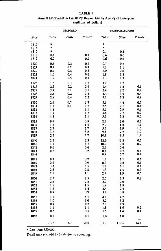
TABLE 4Annual Investment in Canals by Region and by Agency of Enterprise

(millions of dollars)

SEABOARD

Year Total State Private

TRANS-ALLEGHENY

Total State Private

1815 a a

1816 a a

1817 a 0.1 0.11818 0.1 0.1 0.6 0.61819 0.2 0.2 0.6 0.61820 0.4 0.2 0.2 0.7 0.71821 0.4 0.2 0.2 1.1 1.11822 0.7 0.4 0.3 2.0 2.01823 1.0 0.4 0.6 1.8 1.81824 1.2 0.5 0.7 1.3 1.3

1825 1.5 0.3 1.2 1.2 1.21826 2.6 0.2 2.4 1.4 1.3 0.11827 3.2 0.1 3.1 2.4 2.2 0.21828 3.5 0.2 3.3 4.3 3,9 0.41829 2.9 0.4 2.5 4.1 3.3 0.8

1830 2.4 0.7 1.7 5.1 4.4 0.71831 1.3 0.1 1.2 2.5 2.1 0.41832 1.1 1.1 3.5 2.9 0.61833 1.7 1.7 3.6 2.7 0.91834 1.1 1.1 3.3 2.8 0.51835 0.9 0.9 2.6 2.0 0.61836 1.5 1.5 2.9 1.8 1.11837 2.7 2.7 5.5 3.9 1.61838 3.2 3.2 9.1 7.2 1.91839 2.7 2.7 10.9 9.5 1.4

1840 2.3 2.3 12.0 11.3 0.71841 1.7 1.7 10.0 9.8 0.21842 0.6 0.6 2.6 2.61843 0.2 0.2 0.8 0.7 0.11844 0.9 0.7 0.2

1845 0.7 0.7 1.3 1.1 0.21846 0.9 0.9 0.9 0.8 0.11847 3.5 3.5 1.2 1.1 0.11848 2.8 2.8 1.8 1.5 0.31849 1.1 1.1 2.4 1.9 0.51850 2.3 2.3 2.5 2.3 0.21851 2.8 2.8 2.0 2.01852 1.5 1.5 1.9 1.91853 1.4 1.4 2.4 2.41854 0.9 0.9 3.8 3.81855 1.1 1.1 4.2 4.21856 1.0 1.0 3.2 3.21857 0.7 0.7 2.9 2.91858 1.1 1.1 1.8 1.6 0.21859 0.5 0.5 1.5 1.4 0.1

1860 0.1 0.1 1.0 1.0

63.5 3.7 59.8 131.7 117.6 14.1

a Less than $50,000.Detail may not add to totals due to rounding.


APPENDIX ASources

A. GENERAL

George Armroyd, A Connected View of the Whole Internal Navigationof the United States; Natural and Art cial, Present and Prospective,Lydia R. Bailey, 1830.

Archer B. Hulbert, Historic Highways of America, 16 vols., Arthur H.Clark, 1902—05.

Chester L. Jones, The Economic History of the Anthracite TidewaterCanals, J. C. Winston, 1908.

Caroline E. MacGill, Ct a!., History of Transportation in the UnitedStates before 1860, Carnegie Institution of Washington, 1917.

S. A. Mitchell, Mitchell's Compendium of the Internal Improvements ofthe United States: Comprising General Notices of All the MostImportant Canals and Rail-Roads, Mitchell and Hinman, 1835.

Henry V. Poor, History of the Railroads and Canals of the UnitedStates of America, New York, 1860.

Ulrich B. Phillips, A History of Transportation in the Eastern CottonBelt to 1860, Columbia University Press, 1908.

J. L. Ringwalt, Development of Transportation Systems in the UnitedStates, J. L. Ringwalt, 1888.

Harvey H. Segal, "Canal Cycles, 1834—1861: Public ConstructionExperience in New York, Pennsylvania, and Ohio," unpublisheddoctoral dissertation, Columbia University, 1956.

Henry S. Tanner, A of the Railroads and Canals of theUnited States: Comprehending Notices of All the Works of InternalImprovement throughout the Several States, Tanner and Disturnell,1840.

Roads, Canals, and Internal Improvements, 1815-1835, H. R. 850, 24thCong., 1st sess. 1880 Census of the United States, Vol. iv, Trans-portation.

Noble E. Whitford, History of the Canal System of the State of NewYork, supplement to the 1905 Report of the State Engineer, 1906.

B. SPECIFIC

1. Monographs and ArticlesElbert J. Benton, "The Wabash Trade Route in the Development of

the Old North West," Johns Hopkins University Studies in His-torical and Political Science, Vol. xxi, nos. 1—2.

Avard L. Bishop, "The State Works of Pennsylvania," Transactions ofthe Connecticut Academy of Arts and Sciences, Tuttle, Morehouse,and Taylor, 1908.

561

IN VESTMENT

Ernest L. Bogart, Internal Improvements and State Debt in Ohio,Longmans, 1924.

A Century of Progress; History of the Delaware and Hudson Company1823—1923, Delaware and Hudson Company, 1925.

Wayland F. Dunnaway, History of the James River and Kanawha Co.,Columbia University Press, 1922.

Logan Esarey, "Internal Improvements in Early Indiana," IndianaHistorical Society, 1912.

Farmington Canal Company, An Account of the Farmington CanalCompany, of the Hampshire and Hampden Canal Company, and ofthe New Haven and Northampton, till the Suspension of Its Canal in1847, Thomas J. Stafford, 1850.

Clifford R. Hinshaw, Jr., "North Carolina Canals before 1860,"North Carolina Historical Review, January, 1948.

T. B. Klein, "The Canals of Pennsylvania and the System of InternalImprovements," supplement to Report of the Pennsylvania Secretaryof Internal Improvements, 1901.

C. P. McClelland and C. C. Huntingdon, History of the Ohio Canals,Their Construction, Cost, Use and Partial Abandonment, OhioState Archeological and Historical Society, 1905.

Charles N. Morris, "Internal Improvements in Ohio, 1825—1850,"Papers of the American Historical Association, 1889.

James W. Putnam, "The Illinois and Michigan Canal; A Study inEconomic History," Chicago Historical Society's Collections, 1918.

Christopher Roberts, The Middlesex Canal, 1793-1860, Harvard Uni-versity Press, 1938.

Walter S. Sanderlin, The Great National Project: A History of theChesapeake and Ohio Canal, Johns Hopkins Press, 1946.

2. State DocumentsReports (variously titled) of canal commissioners, canal engineers,

state treasurers or comptrollers for: New York, 1816—60; Penn-sylvania, 1826—60; Virginia, 1820—35; South Carolina, 1819—28;Ohio, 1825—60; Indiana, 1833—60; Illinois, 1836-60.

3. Corporate DocumentsReports (variously titled) of: Chesapeake and Delaware, 1824—60;

Chesapeake and Ohio, 1829—60; Cincinnati and Whitewater, 1840;Delaware and Hudson, 1823—60; Delaware and Raritan, 1831—60;James River and Kanawha, 1835-60; Lehigh Coal and NavigationCo., 1827—60; Morris Canal and Banking Co., 1826—60; Penn-sylvania and Ohio, 1835—60; Schuylkill Navigation, 1827—60;Susquehannah and Tidewater, 1844, 52, 53; Union Canal, 1813—60.

562


APPENDIX BCanals Employed in Developing the Average

Expenditure Pattern

Years of CostAgency and Name Construction (millions)

New York State:Erie 1817—27 $7,144Oswego 1825—28 565cayuga and Seneca 1827—29 237Crooked Lake 1830—33 157Chenango 1833—37 2,316Genesee Valley 1837—44 5,663

Pennsylvania:Eastern Division 1826—34 1,347

Juniata Division 1827—34 3,047Western Division 1826—30 2,760Susquehannah Division 1828—33 1,039West Branch Division 1828—33 1,580Delaware Division 1827—30 1,238Beaver Division 1828—33 519

South Carolina:Drehers 1820—22 78Saluda 1819—22 157

Columbia 1820—24 211Broad River 1820—25 111Landsford 1820—26 130Catawba 1820—26 164Wateree 1821—27 158

Ohio:Ohio 1825—34 4,245Miami 1825—31 788

Private:Pennsylvania and Ohio 1835—40 1,135Louisville and Portland 1826-30 1,019

563

IN VESTMENT

APPENDIX CCanals Employed in Multiple Regression Analysis

YearName Costa Lenglhb Prismc Lockage'1 Completed

Cumberland and Oxford 25 21 104 143 1829

Middlesex 53 27 75 136 1804Blackstone 60 45 104 451 1828Hampshire and Hampden 23 22 112 298 1835Farmington 60 56 112 218 1831Erie 714 363 136 676 1827

Champlain 92 66 132 188 1823

Oswego 57 38 132 155 1828

Chemung 31 23 136 395 1833

Chenango 232 97 136 278 1833Genesee Valley 566 114 136 1,045 1857Black River 231 88 132 1,083 1849

Delaware and Hudson 188 108 96 1,073 1829

Delaware and Raritan 284 65 462 116 1834

Morris 311 103 104 1,674 1831

Eastern Division 135 43 287 132 1834

Juniata 305 130 170 615 1830Western 276 104 136 471 1830

Susquehannah 104 39 321 68 1833

West Branch 158 72 180 107 1833

North Branch 140 73 158 90 1830

Upper North Branch 564 103 128 259 1850

Delaware 124 60 165 164 1830Schuylkill 185 110 105 588 1825

Erie Extension 553 163 168 930 1844

Lehigh 156 85 265 353 1829Susquehannah and Tidewater 326 45 215 233 1840

Chesapeake and Delaware 275 14 504 32 1829Chesapeake and Ohio 1,011 185 280 610 1850

James River and Kanawha 126 37 119 237 1827

Albemarle and Chesapeake 164 44 595 2 1858Dismal Swamp 68 30 248 85 1822

Santee 65 22 104 103 1802

Ohio 425 333 132 1,218 1834

Miami 788 244 215 907 1842

Wabash and Erie 633 379 132 505 1851

Illinois and Michigan 656 109 288 141 1848

Wateree 16 4 48 52 1827

Catawba 16 7 48 178 1826

Landsford 13 2 48 32 1826

Broad River 11 3 48 46 1825

Saluda 16 3 48 35 1826

Columbia 21 3 48 36 1826

Rocky Mount 20 5 48 122 1829

Cost—tens of thousands of dollars.b Length—miles.Prism—square feet of cross section.

d Lockage—feet of total rise and fall.

564


COMMENTHARVEY H. SEGAL, New York University

Jerome Cranmer is to be congratulated. He has invaded a territorywhich, until recently, has been the exclusive province of the tow-pathantiquarian, the folklorist, the retired engineer, and the nonquantitativehistorian.

My comments will be directed exclusively to Cranmer's methods ofderiving his annual estimates of investment. His principal finding, thatthere were three long cycles in canal investment, appears to me to bevalid. My objections concern the turning points and the amplitudes ofthose cycles.

Cranmer's estimates of annual investment cover three classes ofcanals, for which there are (1) annual data on construction outlays,(2) only total cost figures, and (3) no data on construction costs. Canalsof the first class—for which there are data on annual construction out-lays—account for about 60 per cent of Cranmer's estimate of totalinvestment. About 90 per cent of the canals in that class were con-structed by state governments. In his estimates of investment in thestate projects, Cranmer relied upon the summary totals of annualexpenditures reported periodically by state commissions; he did notexamine the accounts for individual projects.'

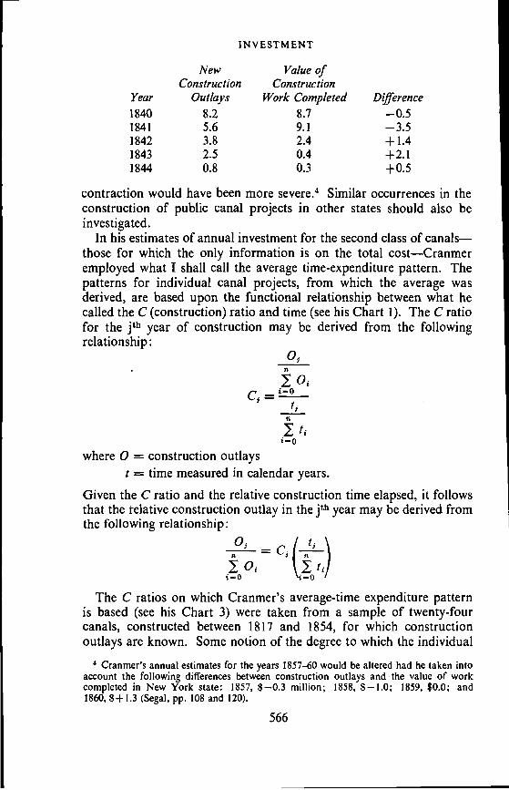
This saved time, but I think the price was rather high. First, thesummary totals include items which cannot be properly classified asconstruction expenditures, and damage payments, which frequentlylagged construction operations by years. Thus Cranmer has probablyoverstated the total investment by some 7 per cent.2 Second, Cranmerimplicitly assumes that annual construction outlays, appearing in thesummary accounts, were equal to the value of construction workcompleted. There were, however, periods of financial difficulty, par-ticularly during the cyclical contraction of 1839—43, when payments tocontractors lagged far behind the pace of construction, and outstandingindebtedness mounted. For the canal systems of New York, Penn-sylvania, and Ohio, the differences between the annual construction out-lays and the value of construction work completed in 1840 44 werevery large, as the table on next page indicates (in millions of dollars).3Had Cranmer taken these data into account, the second canal cyclewould have reached its peak in 1841 instead of 1840, and the ensuing

1 Cranmer explained his procedure in a letter to the writer dated August 6, 1957.2 For the magnitude and composition of such outlays for the canals of the states of

New York, Pennsylvania, and Ohio, see Harvey H. Segal, "Canal Cycles, 1834—1861:Public Construction Experience in New York, Pennsylvania and Ohio," unpublisheddissertation, Columbia University, 1956, pp. 113, 117, 209—210, and 276—277.

These estimates are based upon state documents relating to outstanding debts duecanal contractors. Segal, pp. 119—120, 212, 243, and 278.

565

IN VESTMENT

New Value ofConstruction Construction

Year Outlays Work Completed Dqcference

1840 8.2 8.7 —0.51841 5.6 9.1 —3.51842 3.8 2.4 +1.41843 2.5 0.4 +2.11844 0.8 0.3 +0.5

contraction would have been more severe.4 Similar occurrences in theconstruction of public canal projects in other states should also beinvestigated.

In his estimates of annual investment for the second class of canals—those for which the only information is on the total cost—Cranmeremployed what I shall call the average time-expenditure pattern. Thepatterns for individual canal projects, from which the average wasderived, are based upon the functional relationship between what hecalled the C (construction) ratio and time (see his Chart 1). The C ratiofor the year of construction may be derived from the followingrelationship:

05

Ci

'tii=o

where 0 = construction outlayst = time measured in calendar years.

Given the C ratio and the relative construction time elapsed, it followsthat the relative construction outlay in the jth year may be derived fromthe following relationship:

05

The C ratios on which Cranmer's average-time expenditure patternis based (see his Chart 3) were taken from a sample of twenty-fourcanals, constructed between 1817 and 1854, for which constructionoutlays are known. Some notion of the degree to which the individual

Cranmer's annual estimates for the years 1857—60 would be altered had he taken intoaccount the following differences between construction outlays and the value of workcompleted in New York state: 1857, $—0.3 million; 1858, $—1.0; 1859, $0.0; and1860,$+l.3(Segal,pp. 108 and 120).

566


patterns were smoothed in the single average pattern may be had bycomparing Cranmer's Charts 2 and 3. A measure of dispersion, suchas the average deviation of value about each C point in the averagepattern, would have been helpful.

Assuming there were no appreciable payment lags or cessations ofconstruction operations, the average time-expenditure pattern has acertain intuitive appeal.5 Under certain restrictive conditions, it isreasonable to assume that the average time-expenditure pattern foruninterrupted canal construction will ascribe over time a polygon-likecurve skewed to the right. Such a pattern merely indicates that con-struction outlays are relatively small during the early stages of work,that they reach a peak before half of the construction period has elapsed,and that they decline as the last details of a canal are completed.

However, an average-time expenditure pattern such as Cranmer hasemployed does not yield tolerably accurate estimates over forty-fiveyears unless one can safelyassume that: the time-expenditure patternsfor long and short canals have shapes that are essentially alike; notechnological changes take place over the period to which the pattern isto be applied; and construction costs remain constant.

I strongly suspect that there may be systematic differences in theshapes of the time-expenditure patterns for long and short canals, andthat this accounts for a large part of the variation in the shapes of thepatterns for the six New York State canals (Cranmer's Chart 2). The"clean-up" operations on a canal, including the sealing of leaks in themost recently flooded sections, would be an example of different time-expenditure patterns for long and short canals. The range of variationof mileage for the six canals is 358 miles.6

While no striking technological changes, such as the use of steamshovels, occurred during Cranmer's period, canal contractors in the late1840's and the 1850's enjoyed substantial external economies whichgave them a decided advantage over their predecessors. Stone quarriesbecame more numerous and transport facilities were often superior.These factors must have affected the shapes of the time-expenditurepatterns.

Finally, canal construction costs fluctuated widely, particularlybetween 1834 and 1860. Data on total construction costs are scarce, butthe available evidence indicates that total construction costs rose by atleast 33 per cent between 1836 and 1839 and then declined sharply after1842 when most construction activity ceased.7 Rising constructioncosts would tend to truncate the right-hand tail of the time-expenditure

Work on one of the twenty-four canals in Cranmer's sample, the Genesee Valley Canalof New York, was interrupted for six years between 1841 and 1847. It is difficult to appraisethe effects of the inclusion of that canal on the average time-expenditure pattern.

° The Crooked Lake canal was only eight miles long; the Erie was 363 miles long.See Segal, pp. 44, 201, and 296—297.

567

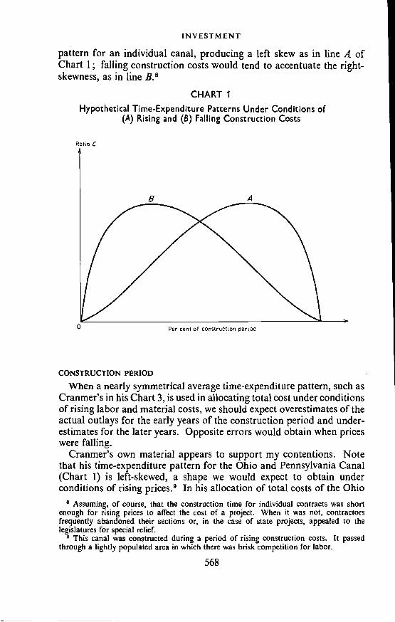
IN VESTMENT

pattern for an individual canal, producing a left skew as in line A ofChart 1; falling construction costs would tend to accentuate the right-skewness, as in line B.8

CHART I

Hypothetical Time-Expenditure Patterns Under Conditions of(A) Rising and (B) Falling Construction Costs

Rotio C

0

CONSTRUCTION PERIODWhen a nearly symmetrical average time-expenditure pattern, such as

Cranmer's in his Chart 3, is used in allocating total cost under conditionsof rising labor and material costs, we should expect overestimates of theactual outlays for the early years of the construction period and under-estimates for the later years. Opposite errors would obtain when priceswere falling.

Cranmer's own material appears to support my contentions. Notethat his time-expenditure pattern for the Ohio and Pennsylvania Canal(Chart 1) is left-skewed, a shape we would expect to obtain underconditions of rising prices.9 In his allocation of total costs of the Ohio

8 Assuming, of course, that the construction time for individual contracts was shortenough for rising prices to affect the cost of a project. When it was not, contractorsfrequently abandoned their sections or, in the case of state projects, appealed to thelegislatures for special relief.

This canal was constructed during a period of rising construction costs. It passedthrough a lightly populated area in which there was brisk competition for labor.

568

A

Per cent of construction period


and Pennsylvania (Chart 4), the pattern of the errors is in accord withmy expectations. Also, the errors of estimation for 1837 and 1839 arevery large; expressed as percentages of actual outlays (disregardingsigns) they amount to 22 per cent and 53 per cent, respectively.'0

Although Cranmer did not prepare an annual breakdown of theallocated component of his estimates, we may assume that it is approxi-mately equal to the ratio of "private" canal investment to the total(columns 1 and 3 of Table 3). That ratio varied from 16 per cent in1841 to 100 per cent in 1816, and for the entire period, the ratios weredistributed as follows:

Percentage of Private Number ofInvestment to Total YearsLess than 20 720 and less than 30 1230 and less than 40 540 and less than 50 1150 and less than 60 660 and less than 70 2Over 70 2

Total 45

Given sizable errors of allocation for individual canals, their relativeimportance in the annual totals will be equivalent to the ratio of theallocated component to the total shown above. The absolute magnitudeof the errors will depend upon the total investment in a given year andon the proportion of the total that was derived by allocating total costs.The twenty-one years for which Cranmer estimated 40 per cent or moreof the total investment by the allocating method account for $91,240,000,or more than 46 per cent of the grand total of investment. Differencesin the direction of the errors could reduce the total error for a givenyear, but in the absence of detailed information it is impossible to sayhow important the offsetting might be.

For the last class of canals—for which there was no information oncosts—Cranmer first estimated the total cost by means of a multipleregression equation and then used his average time-expenditure patternto derive annual estimates. In deriving the regression equation, he useddata on the physical characteristics of forty-four canals constructedbetween 1804 and 1857. His dependent variable, total cost, is expressedin current prices, and as a consequence it is difficult to evaluate hisestimate of the total costs of canals, for which there is no information.Presumably, the resulting cost estimates represent some weighted

10 In his Chart 4, Cranmer did not "level-up" the annual C ratios so that they total six.If that correction is made, the errors are 25 per cent and 49 per cent, respectively.

569

INVESTMENT

average of the construction cost levels between 1804 and 1857. Also,two of Cranmer's three independent variables, prism size and lockage,are of questionable value. Prism designs varied among canal projects;those lined with masonry henchwalls, as on the enlarged Erie Canal,cost far more than ordinary prisms of the same size. Locks varied indesign, construction, and size of lock chambers, with resultant differ-ences in construction costs.

I should like to suggest these improvements in Cranmer's estimates:1. Construction of a separate annual series of estimates of investment

in canals for which annual construction outlays are known, withadjustments for periods in which payments lagged behind the value ofconstruction work completed. Such a series would be valuable in theanalysis of cycles, and in dating their turning points. The annual totalswould probably represent the bulk of canal investment for most years.

2. Tests of possible systematic variations in the time-expenditurespatterns of large and small canals, and of canals of approximately thesame size built in different periods.

A more difficult problem is posed by changes in construction costs.First, Cranmer might compile a canal-construction cost index withwhich to deflate the estimates yielded by the appropriate average time-expenditure pattern. Before applying such a deflator, he would need toknow the average duration of construction contracts. Second, if suchan index cannot be constructed, he might alter the shape of the time-expenditure curve to make rough allowances for changes in costs whereonly the direction of the change is known. The accuracy of thesemanipulations could be tested by applying them to the total costs ofcanals for which there is information on annual construction outlays.

3. No attempt should be made to estimate the total costs of canalsfor which there is no information unless the cost data used in theestimating equation can be deflated and the dependent variables can beexpressed in a more satisfactory form.

570