Embed Size (px)
Citation preview

Glasgow Theses Service http://theses.gla.ac.uk/
Canamar Leyva, Alan Leonel (2012) Seaplane conceptual design and sizing. MSc(R) thesis. http://theses.gla.ac.uk/4030/ Copyright and moral rights for this thesis are retained by the author A copy can be downloaded for personal non-commercial research or study, without prior permission or charge This thesis cannot be reproduced or quoted extensively from without first obtaining permission in writing from the Author The content must not be changed in any way or sold commercially in any format or medium without the formal permission of the Author When referring to this work, full bibliographic details including the author, title, awarding institution and date of the thesis must be given

Seaplane Conceptual Design and Sizing by
Alan Canamar
A thesis submitted to the School of Engineering,
University of Glasgow in
fulfillment of the requirements of
the degree of Master of Science
Aerospace Sciences
Supervisor: L. Smrcek
November 2012

ii
Abstract Ever since the idea of flying machines that could land and take off from water (seaplanes) was
invented in 1910, a huge amount of research was poured into it until it stagnated in 1950. Their
performance did not grow according to current aircraft requirements. The idea of designing
advance seaplane concepts stopped, and most seaplanes existing these days are approaching their
final operating life. The purpose of this research project was to introduce a new seaplane concept
design methodology that will suffice the necessities of actual aircraft designers. This concept
design replaces old sizing methods proposed with a more efficient methodology based on
modern aircraft design methods. The sizing method developed gives the designer a “freedom” in
creating an “out of the box” seaplane concept. The optimization method was elaborated in such a
manner that the designer can use certain types of aircraft configuration (Conventional, Blended
Wing Body, and Flying Wing). The sizing method simplified the design by calculating the most
advanced floating device for this seaplane concept. Old seaplane information was blended with
modern aircraft and modern ship design information, creating a new preliminary seaplane
concept design. Another advantage of this design method is the idea to convert existing
landplane into a seaplane by adding the floating device that meets the necessary requirements of
the seaplane conversion.
The second part of the research was to address technical solutions to the actual seaplane
design. For example, adding a trimaran configuration that increased the hydrodynamic
performance and the use of a retractable float system that reduced aerodynamic drag during
flight. Final results were elaborated to compare the use of trimaran with other types of floating
devices. The final results showed the trimaran concept gave an excellent hydrostatic stability, a
greater water speed, and retracting the floats decreased the aerodynamic drag, hence better flight
performance.
Aircraft design has been affected by actual economical difficulties showing no radical
progress in this field of study. The next purpose of the research was to explore more radical,
environmentally efficient, and innovative technologies. With the aid of the proposed sizing
methodology for a modern and futuristic seaplane, a new vision was created called: 2050
Visionary Aeronautical Design Concept. Based on this vision the creation of an advance “out of
the box” amphibian aircraft was elaborated. The project analyzed technical solutions, and a
conceptual design concept for the creation of this 2050 amphibian aircraft. The preliminary
design development leads to the creation of an Advance Amphibian Blended Body Wing
Aircraft (AABWBA). AABWBA excels in air performance due to the high results generated by
the Blended Wing Body (BWB) Aircraft. Adopting modern turbofan engines instead of
turboprop engines gave the AABWBA better water takeoff capability, as well as air
performance. Modern ideas for 2050 vision are the creation of futuristic seaports in order to
increase seaplane traffic, public and commercial awareness, and expand market schemes.
A design analysis was performed to show a model representation of this advance seaplane
design. A Computer Aided Design (CAD) model was elaborated to calculate the dimensions,
observe the mechanism of the retractable floats, and show the location of the boat hull. With the
aid of this CAD model, Finite Element Analysis (FEA) was performed to show the structural
strength and impact of the hull and floats when landing on water. Finally, with the aid of this
model, a hydrostatic analysis of the seaplane was conducted to show the water stability, and heel
turns to observe the performance of the trimaran and the retractable floats when the seaplane is
being operated in water.

iii
Acknowledgments I want to give a special thanks to my supervisor, Dr. Ladislav Smrcek, for all his
collaboration, support, and help throughout this project. Also a special gratitude to the University
of Glasgow for the support on equipment and facilities provided in order to conduct this MSc
Research Project.
I will like to thank the collaboration of Mr. Ludovit Jedlicka, Undergraduate student of VSVU
Bratislava (Slovakia) for elaborating the futuristic images of the LET L-410, the Antonov AN-
28, and the BAe 146. Also, to Dr. Gerardo Aragon for his knowledge and guidance in the
elaboration of the optimization sizing code.
Lovely thanks to my partner and wife, Paulina Gonzalez, for all of her help, patience and trust
she gave me during this trip where I came to gain more knowledge and advice from the best
educators. For her calming words and knowledgeable guidance throughout this project that
always kept me on visualizing the objective of finishing this MSc Research.
Last, thanks to all of my friends and family that gave me advice, guidance, support, and
company during this research project.

iv
Table of Contents
Abstract .......................................................................................................................................... ii
Acknowledgments ........................................................................................................................ iii
List of Figures .............................................................................................................................. vii
List of Tables ................................................................................................................................ ix
Nomenclature ................................................................................................................................ x
1. Introduction ............................................................................................................................ 1
1.1. History .............................................................................................................................. 1
1.1.1. 1903 – 1950 .................................................................................................................. 1
1.1.2. 1950 – 1980 .................................................................................................................. 3
1.1.3. 1980 – Present .............................................................................................................. 3
1.2. Seaplane Aircraft Design ................................................................................................. 5
1.3. Seaplane Traffic and Operations ...................................................................................... 6
1.4. Strengths, Weaknesses, Opportunities, and Threats (SWOT) ......................................... 8
1.4.1. Strengths ....................................................................................................................... 8
1.4.2. Weaknesses ................................................................................................................. 10
1.4.3. Opportunities .............................................................................................................. 10
1.4.4. Threats ........................................................................................................................ 11
2. Literature Review ................................................................................................................. 12
2.1. Aircraft Design ............................................................................................................... 12
2.1.1. Examples of Existing Landplane for Seaplane Conversion ....................................... 13
2.2. Water Operation Design ................................................................................................. 14
2.2.1. Hydrodynamic Shape Characteristics ......................................................................... 14
2.2.2. Boat Hull Design ........................................................................................................ 17
2.2.3. Float Design ................................................................................................................ 17
2.2.4. Trimaran and Retractable Float System ..................................................................... 18
3. Advance Seaplane Conceptual Optimization Method ...................................................... 23
3.1. Conceptual Design ......................................................................................................... 23
3.2. Sizing Code Development and Validation ..................................................................... 24
3.2.1. Landplane Optimized Testing Source Code (LOTS) ................................................. 25
3.2.2. Floating Device Optimized Testing Source Code (FOTS) ......................................... 26
3.2.3. Validation ................................................................................................................... 28
3.3. Theory ............................................................................................................................ 29

v
3.3.1. Aeronautical Theory ................................................................................................... 29
3.3.2. Naval Architecture Theory ......................................................................................... 33
4. Results ................................................................................................................................... 40
4.1. Landplane Results .......................................................................................................... 40
4.1.1. Geometry .................................................................................................................... 40
4.1.2. Empty Weight ............................................................................................................. 41
4.1.3. Aerodynamic Drag ..................................................................................................... 41
4.1.4. Flight Performance ..................................................................................................... 43
4.2. Floating Device Results ................................................................................................. 47
4.2.1. Weight Breakdown ..................................................................................................... 47
4.2.2. Geometry calculations ................................................................................................ 47
4.2.3. Hydrostatic Stability ................................................................................................... 50
4.2.4. Water Takeoff Requirements ...................................................................................... 51
4.2.5. Aerodynamic Drag ..................................................................................................... 52
4.2.6. Flight Performance ..................................................................................................... 54
4.3. Design Analysis.............................................................................................................. 57
4.3.1. SOLIDWORKS Computer Aided Design (CAD) Analysis ....................................... 57
4.3.2. ORCA 3D ................................................................................................................... 59
4.3.3. Software Validation .................................................................................................... 62
5. 2050 Visionary Concept: Future Seaplane Transport ...................................................... 63
5.1. Introduction .................................................................................................................... 63
5.2. Review of Literature....................................................................................................... 63
5.3. Design Selection ............................................................................................................. 64
5.3.1. Input Parameters ......................................................................................................... 64
5.3.2. Fuselage Thickness ..................................................................................................... 65
5.3.3. Airfoil ......................................................................................................................... 65
5.3.4. Wing Sweep (Λ) ......................................................................................................... 65
5.4. Preliminary Results ........................................................................................................ 66
5.4.1. Geometric Properties (BWB) ..................................................................................... 67
5.4.2. Weight Breakdown ..................................................................................................... 68
5.4.3. Control Surfaces ......................................................................................................... 68
5.4.4. Trimaran Dimensions ................................................................................................. 69
5.4.5. Hydrostatic Stability ................................................................................................... 70
5.4.6. Water Resistance ........................................................................................................ 70

vi
5.4.7. Air Performance ......................................................................................................... 71
5.5. Summary ........................................................................................................................ 73
6. Conclusions and Recommendations ................................................................................... 75
6.1. Conclusions .................................................................................................................... 75
6.2. Recommendations .......................................................................................................... 76
6.2.1. Sizing Code Improvements ........................................................................................ 76
6.2.2. Technical Improvements ............................................................................................ 76
References .................................................................................................................................... 79
Appendix ...................................................................................................................................... 82
Appendix A. Empirical Equations ............................................................................................. 82
A.1 Empty Weight Breakdown Equations ........................................................................ 82
A.2 Flat Plate Drag Area Breakdown Equations ............................................................... 83
A.3 Aircraft Flight Performance Equations....................................................................... 85
A.4 Hull geometrical empirical formulas .......................................................................... 88
Appendix B. Artistic impressions of the conversion of current certified aircraft to a seaplane 89
Appendix C. MATLAB Optimization Source Code ................................................................. 90

vii
List of Figures
Fig. 1: Le Canard [2] ....................................................................................................................... 2 Fig. 2: The Flying Fish [2] .............................................................................................................. 2 Fig. 3: Navy Curtiss [5] .................................................................................................................. 2 Fig. 4: Short S-23 Empire [6] ......................................................................................................... 2 Fig. 5: Sikorsky S-42 [2] ................................................................................................................. 3 Fig. 6: Martin M130 [2] .................................................................................................................. 3 Fig. 7: Hughes H-4 Hercules “Spruce Goose” [7] .......................................................................... 3 Fig. 8: Expeditionary fighting vehicle [8]...................................................................................... 4 Fig. 9: Lun-class Ekranoplan [9].................................................................................................... 4 Fig. 10: Do.24 ATT [9] ................................................................................................................... 4 Fig. 11: Canadair CL-415 [11]........................................................................................................ 4 Fig. 12: Beriev Be-103 [12] ............................................................................................................ 5 Fig. 13: Beriev Be-200 [12] ............................................................................................................ 5 Fig. 14: Average Percentage Growth of Travel in the UK [13] ...................................................... 7 Fig. 15: Seaport in Vancouver Harbor, Canada [15] ...................................................................... 7 Fig. 16: Design Features of a Flying Boat [27] ............................................................................ 14 Fig. 17: Beam Width of a Conventional Boat [36] ....................................................................... 15 Fig. 18: Various Types of Boat Hull Bottoms [41] ...................................................................... 16 Fig. 19: Hydrofoil Example [53] .................................................................................................. 18 Fig. 20: Trimaran Example [55] ................................................................................................... 19 Fig. 21: Trimaran Stability-Beam Model [56] .............................................................................. 19 Fig. 22: Resistance comparison curves [57] ................................................................................. 20 Fig. 23: Trimaran coordinate Axis [56] ........................................................................................ 20 Fig. 24: Outrigger stagger and clearance [56] .............................................................................. 21 Fig. 25: Retracting Float Concept [59] ......................................................................................... 22 Fig. 26: Example CAD Model with Floats retracted inside Hull ................................................. 22 Fig. 27: Heel Overturn Retracting Float System .......................................................................... 22 Fig. 28: Seaplane Design Optimization Method Flow Chart ........................................................ 24 Fig. 29: Flowchart of the LOTS architecture ................................................................................ 26 Fig. 30: Flowchart of FOTS architecture ...................................................................................... 27 Fig. 31: Input Landplane Characteristics ...................................................................................... 27 Fig. 32: Slenderness Ratio ............................................................................................................ 35 Fig. 33: Wing Tip Floats [42] ....................................................................................................... 35 Fig. 34: Transverse Metacentric Height [45] ................................................................................ 37 Fig. 35: Wave Making Resistance [67]......................................................................................... 38 Fig. 36: Deadrise Angle [67] ........................................................................................................ 39 Fig. 37: 3-D CAD Model of Conventional Landplane Aircraft .................................................... 41 Fig. 38: Drag Curves (Landplane) ................................................................................................ 42 Fig. 39: Thrust Curves (Landplane) .............................................................................................. 42 Fig. 40: Landplane Climb Diagram .............................................................................................. 44 Fig. 41: Altitude Envelope of Landplane ...................................................................................... 44 Fig. 42: Payload Range Diagram (Landplane) ............................................................................. 46 Fig. 43: Maneuvering and Gust Envelopes (Landplane) .............................................................. 46 Fig. 44: Water Landing Load Factor Curve .................................................................................. 49

viii
Fig. 45: CAD Model of Seaplane with Wing Tip Floats .............................................................. 49 Fig. 46: CAD Model of Seaplane with Nacelle Support Stabilizers ............................................. 49 Fig. 47: CAD Model of Seaplane with Trimaran Concept ........................................................... 50 Fig. 48: CAD Model of Seaplane transverse Metacentre, Centre of Gravity, and Buoyancy ...... 50 Fig. 49: Righting Moment Graph.................................................................................................. 51 Fig. 50: Water Resistance Curves and Thrust Available .............................................................. 52 Fig. 51: Wing Tip Floats Retracted into the Wing Tip ................................................................. 52 Fig. 52: Nacelle Wing Stabilizers Retracted ................................................................................. 53 Fig. 53: Trimaran Outriggers Retracted unto the Boat Hull ......................................................... 53 Fig. 54: Thrust Curves (Landplane and Trimaran Seaplane) ........................................................ 55 Fig. 55: Altitude Envelope (Landplane and Trimaran Seaplane [Retracted]) .............................. 55 Fig. 56: Payload Range Diagram (Landplane and Trimaran Seaplane [Retracted]) .................... 56 Fig. 57: Maneuvering and Gust Envelopes (Trimaran Seaplane) ................................................. 56 Fig. 58: Trimaran Seaplane Fuselage Fixture ............................................................................... 58 Fig. 59: Trimaran Seaplane Load Force at Afterbody Hull .......................................................... 58 Fig. 60: Trimaran Seaplane Mesh ................................................................................................. 59 Fig. 61: Trimaran Seaplane Von Mises Stress Analysis ............................................................... 59 Fig. 62: Personal Watercraft Modeled as a NURBS and a T-Spline [69] .................................... 60 Fig. 63: Orca3D Results with Virtual Waterline of Trimaran Seaplane (Longitudinal) .............. 61 Fig. 64: Orca3D Results with Virtual Waterline of Wing Tip Floats Seaplane (Transverse) ...... 61 Fig. 65: Trimaran Seaplane at 12
o Heel Angle before Overturning ............................................. 62
Fig. 66: Trimaran Seaplane at 20o Heel Angle before Overturning ............................................. 62
Fig. 67: Example Blended Wing Body Aircraft [70] .................................................................... 64 Fig. 68: Top-down view of BWB showing wing and wing fences ............................................... 66 Fig. 69: Blended Wing Body Aircraft ........................................................................................... 66 Fig. 70: Cut view of BWB fuselage .............................................................................................. 67 Fig. 71: BWB fuel tanks ............................................................................................................... 68 Fig. 72: Top view of BWB with control surfaces labeled ............................................................ 69 Fig. 73: CAD Model of AABWBA .............................................................................................. 70 Fig. 74: Metacentric Height of AABWBA ................................................................................... 70 Fig. 75: Resistance Curves AABWBA ......................................................................................... 71 Fig. 76: Altitude Envelope of BWB and AABWBA .................................................................... 72 Fig. 77: Payload Range Diagram .................................................................................................. 72 Fig. 78: Maneuvering and Gust Envelopes ................................................................................... 73 Fig. 79: AABWBA at takeoff from seaport .................................................................................. 74 Fig. 80: AABWBA taxing at seaport ............................................................................................ 74 Fig. 81: Futuristic CAD Model of Amphibians at a Modern Sea Port ......................................... 77 Fig. 82: Futuristic CAD Model of a Turboprop Seaplane and AABWBA ................................... 78 Fig. 83: Futuristic CAD Model of AABWBA at taxi ................................................................... 78 Fig. 84: Artistic Impression of LET L-410 [75] ........................................................................... 89 Fig. 85: Artistic Impression of Antonov AN28 [75]..................................................................... 89 Fig. 86: Artistic Impression of BAE 146 [75] .............................................................................. 89 Fig. 87: Artistic Impression of Dornier DO-228 [75] ................................................................... 89

ix
List of Tables
Table 1: Noise levels for various operations [18] ........................................................................... 9 Table 2: Aircraft Specifications .................................................................................................... 13 Table 3: LOTS Comparison Validation ........................................................................................ 28 Table 4: FOTS Comparison Validation ........................................................................................ 28 Table 5: Spray Coefficient Factors ............................................................................................... 35 Table 6: Geometrical Parameters of Landplane ............................................................................ 40 Table 7: Empty Weight Breakdown (Landplane) ......................................................................... 41 Table 8: Flat Plate Drag Area Breakdown (Landplane) ............................................................... 43 Table 9: Endurance and Range (Landplane) ................................................................................. 45 Table 10: Weight Component Breakdown ................................................................................... 47 Table 11: Floating Device Dimensions......................................................................................... 48 Table 12: Hydrostatic Stability (Seaplane) ................................................................................... 50 Table 13: Flat Plate Drag Area Breakdown Floating Devices ...................................................... 54 Table 14: Flat Plate Drag Area Breakdown Trimaran Seaplane ................................................... 54 Table 15: Endurance and Range of each Flight Segment ............................................................. 55 Table 16: Summary of major design values (Landplane and Trimaran Seaplane) ....................... 57 Table 17: Blended Wing Body Parameters ................................................................................... 66 Table 18: BWB and AABWBA Weight Breakdown ................................................................... 68 Table 19: Trimaran Dimensions (AABWBA) .............................................................................. 69 Table 20: Flat Plate Drag Area Breakdown Component .............................................................. 71 Table 21: Summary of major design values (BWB and AABWBA) ........................................... 74
x
Nomenclature
A = Area of Load Water Plane [m2]
AR = Aspect Ratio
b = Wing Span [m]
BG = Distance from Center of Buoyancy to Center of Gravity [m]
bh = Boat Hull Beam [m]
BM = Reduction in Metacentric Height [m]
BPR = Bypass Ratio
c = Mean Wing Chord Length [m]
CD = Total Drag Coefficient
CDi = Coefficient of Induced Drag
CDp = Coefficient of Parasite or Viscous Drag
CDw = Coefficient of Wave or Compressibility Drag
Cf = Friction Coefficient
cHT = Horizontal Tail Volume Coefficient
CL = Coefficient of Lift
cr = Wing Root Chord [m]
CRM = Righting Moment Coefficient
CRw = Coefficient of Water Resistance
ct = Wing Tip Chord [m]
Cv = Coefficient of Water Viscous Resistance
cVT = Vertical Tail Volume Coefficient
Cw = Coefficient of Water Wave Resistance
C1 = Seaplane Operation Factor
= Static Beam Load Coefficient
D = Total Aerodynamic Drag [N]
Di = Induce Aerodynamic Drag [N]
Dp = Parasite Aerodynamic Drag [N]
Dw = Wave or Compressibility Drag [N]
E = Endurance [hr]
e = Oswald’s efficiency factor
EW = Empty Weight [kg]
EWl = Empty Weight of Landplane [kg]
EWs = Empty Weight of Seaplane [kg]
F = Form Factor
f = Flat Plate Drag Area [m2]
FC = Fuel Consumption [kg/sec]
fth = Throttle Setting
g = Gravitational Acceleration [m/s2]
GM = Metacentric Height [m]
GW = Total Gross Weight of Aircraft [kg]
GWest = Estimated Gross Weight [kg]
I = Moment of Inertia [m4]
K = Geometrical Form Factor of Floating Device
k = Spray coefficient

xi
L = Lift [N]
l = Distance from the lateral stabilizer to the center of the fuselage [m]
la = Afterbody Length of Boat Hull [m]
lf = Forebody Length of Boat Hull [m]
Lh = Length of Boat Hull [m]
LHT = Horizontal Tail Moment Arm [m]
LVT = Vertical Tail Moment Arm [m]
M = Mach number
Mdiv = Divergence Mach number
mf = Fuel Mass [kg]
MR = FAA Righting Moment [N-m]
n = Number of Floats or Stabilizers
nw = Water Landing Load Factor
Q = Interference Factor
q = Dynamic Pressure [Pa]
R = Range [km]
Re = Reynolds Number
RM = Righting Moment [N-m]
Rw = Water Resistance [N]
S = Planform Wing Area [m2]
SHT = Horizontal Tail Planform Area [m2]
SLR = Slenderness Ratio
SVT = Vertical Tail Planform Area [m2]
Swet = Wetted Wing Area [m2]
t = Time [sec]
TA = Available Thrust [N]
TR = Required Thrust [N]
tsfc = Thrust Specific Fuel Consumption [N-kg/hr]
T0 = Static Sea Level Thrust [N]
U = Volume [m3]
V = Velocity [m/s]
Vc = Climb Speed [m/s]
Vso = Stall Speed [m/s]
VTAS = True airspeed [m/s]
W = Weight [kg]
w = Density of Water [kg/m3]
Wbh = Boat Hull Weight [kg]
Wf = Weight of one Float [kg]
Wfi = Final Cruise Weight [kg]
Wi = Initial Cruise Weight [kg]
WWT = Wing Stabilizer Weight [kg]
β = Forebody Deadrise Angle [deg]
γ = Heat capacity ratio of air (1.4)
= Angle of Heel Inclination [deg]
ϑ = Temperature Ratio
λ = Taper ratio

xii
ρ = Density of Air [kg/m3]
= Weight Water Displacement [kg]
Λ = Wing Sweep at 25% Mean Aerodynamic Chord (MAC) [deg]
All dimensions are in metric system unless specified

1
1. Introduction
ince the creation of the world’s first successful airplane done by the Wright Brothers in 1903,
the idea for improving and exploring the world of aeronautics have been expanding rapidly
throughout the 20th
century. Aircraft design is the process between many competing factors and
constraints accounting for existing designs and market requirements to produce the best aircraft
[1]. The expansion in aircraft design allowed a wider perspective into analyzing efficient
methods of transportations such as the use of versatile vehicles. There is a design of such
versatile vehicles that had existed for decades, amphibious aircraft. Henry Fabre created the first
motor seaplane flight in 1910 [2], and since then, much research on seaplane aviation was widely
conducted. However, with the concept to improve aircraft designs and the construction of
suitable landplane infrastructure, the use of seaplane traffic and operations drastically dropped
[3]. Current designs are obsolete, and updates to these vehicles have stagnated. The most
important role that seaplanes have today is to conduct fire fighter operations as water bombers;
they are also commonly used in the private sector, in which most seaplanes are just small
landplanes adapted with floats. The lack of an advance seaplane design has pushed the
boundaries into creating a new optimization conceptual design method. The design methodology
complies with the necessities of the actual aviation market schemes and will continue to compete
in the future, both at a short and long term period.
1.1. History
1.1.1. 1903 – 1950
With the lack of suitable landplane infrastructure and the availability of vast motor boats, the
idea of creating a seaplane was born. The first motor seaplane flight was conducted in 1910 by a
French engineer Henry Fabre [2] naming this machine ‘Le canard’ shown in Fig. 1. Since then,
much research on seaplane aviation is widely conducted.
These experiments were followed by the aircraft designers Gabriel and Charles Voisin. They
adapted a number of Fabre’s floats and fitted them into an improved design - the Canard Voisin
airplane. The Canard Voisin airplane became the first seaplane to be used in military exercises
from a seaplane carrier, La Foudre ('the lightning'), in march 1912 [4].
In the United States (US), early development was carried out by Glenn Curtis who worked in
association with Alexander Graham Bell in the Aerial Experiment Association (AEA). His first
seaplane, nickname “Hydroaeroplane”, took off from the San Diego bay on January 26, 1911.
Another model by Curtiss nicknamed as “The Flying Fish” took flight in 1912 shown in Fig. 2.
This prototype faced problems at takeoff during its initial run due to suction forces. Curtis
decided to implement the step, separating the forebody from the afterbody becoming the first
seaplane to demonstrate the advantages of the step [5]. The first British seaplane flight, by
Sydney Sippe, also took place in 1912 [2].
During the periods of the Great War (WWI) (1914-1918), the lack of landplane airfields, and
the availability of controlling key water military points made seaplanes an indispensable tool.
The Curtiss float planes were the only US designated float planes to see combat in WWI. In
1919, the huge flying boat “Navy-Curtiss” shown in Fig. 3, made the first staged aerial crossing
of the Atlantic [5].
S

2
Fig. 1: Le Canard [2]
Fig. 2: The Flying Fish [2]
In the period of post WWI (1918-1939), prospects of the seaplane as a commercial transport
vehicle began to fade and the military began to take over. This dream for commercial seaplane
transport was hijacked by the military, but some airlines still saw significant promise and
potential in seaplanes for long haul travel. Thus, in the late 1930s, forty-two Short Bros' S23 C
Empire Flying-Boats shown in Fig. 4 were built at Rochester, England, to be in service during
the last days of the British Empire, ending its service in June 1940 [6].
During World War II (WWII) (1939 – 1945), seaplanes continued to play an important role in
military aircraft service. In addition to operating with airlines such as Imperial Airways, BOAC,
Qantas and TEAL, the big Sunderlands also saw action with Allied air forces. Across the
Atlantic, Pan America was building up its transpacific routes with its large and impressive
Clipper fleet. The first two trans-Pacific seaplanes were the Sikorsky S-42 and the Martin M130,
Fig. 5 and Fig. 6 respectively, but they were superseded by the Boeing B-314 [2]. In 1942, with
the loss of many cargo ships in the Atlantic Ocean caused by German U-Boats, the U.S. War
Department approved the construction of a transport aircraft that will move the material to Great
Britain. The approved aircraft is the largest seaplane ever constructed, the Hughes H-4 Hercules
“Spruce Goose”, shown in Fig. 7 [7]. However, the H-4 Hercules was completed until 1947, and
only one prototype was made.
Fig. 3: Navy Curtiss [5]
Fig. 4: Short S-23 Empire [6]

3
Fig. 5: Sikorsky S-42 [2]
Fig. 6: Martin M130 [2]
Fig. 7: Hughes H-4 Hercules “Spruce Goose” [7]
1.1.2. 1950 – 1980
Sadly, by the end of WWII, the flying boat industry drastically declined with the increase in
landplane range and speed, coupled with a world-wide network of airfields; though the US Navy
continued to operate some seaplanes. The jet powered seaplane bomber “Martin Seamaster” and
the “Martin P5M Marlin” were among a few that were operated by the Navy, whose operation
continued till the early 1970’s. In defiance to the changing trends, in 1948, Aquila Airways was founded to serve destinations
that were still inaccessible to land-based aircrafts. This company operated “Short S.25” and
“Short S.45” flying boats out of Southampton on routes to a number of remote locations [6].
From 1950 to 1957, Aquila also operated a service from Southampton to Edinburgh and
Glasgow. The airline ceased its operations on 30 September 1958. The aerospace industry was
preoccupied with the research and development of land planes, the enthusiasm resulting from the
expanding spans of commercial air transport, defense and because of certain drawbacks of the
obvious aerodynamic compromises that the seaplanes had relative to landplanes.
1.1.3. 1980 – Present
The dormant era of seaplanes continued till the mid 1980’s until the idea resurged as a part of
the bigger concept of Advanced Amphibious Vehicles (AAV) [8]. AAV are types of transport
vehicles that are able to operate on land as well as on water, an example shown in Fig. 8. The
U.S. military designed AAV in order to deploy troops rapidly from an amphibious assault ship

4
onto land. These military applications revived the idea for designs that could be used by civilian
transport. Sporting activities and leisure travel resumed their roles of bolstering seaplanes in the
market. Another factor that played hugely to the advantage of the seaplane industry was the
introduction of the concept of Wing in Ground effect vehicles (WIG) [9]. The Russian
Ekranoplan, shown in Fig. 9, for instance was one such vehicle. It was not only designed to
minimize drag, but also to work some of the aerodynamic lift forces to its advantage. These
vehicles continue to influence yacht and ship designs for high speed cruising and sailing.
Presently similar research is being poured into seaplanes in order to improve their performance
in high waves and rough weather conditions.
There are a few seaplane companies that excel in some advance designs. Some companies are
Dornier and Canadair with the introduction of models like Do.24 ATT [9] and CL-415 [11], Fig.
10 and Fig. 11 respectively. Beriev Aircraft Company is a Russian amphibious aircraft
manufacturer with its two most noticeable seaplanes, the Beriev Be-103 Fig. 12 and Beriev Be-
200 Fig. 13 [12].
The time table shows the technological improvements of different type of seaplanes that were
made throughout the century. Such improvements are to be brought about by paying attention to
the obvious drawbacks that the seaplane suffers from despite its improved designs.
Fig. 8: Expeditionary fighting vehicle [8]
Fig. 9: Lun-class Ekranoplan [9]
Fig. 10: Do.24 ATT [9]
Fig. 11: Canadair CL-415 [11]

5
Fig. 12: Beriev Be-103 [12]
Fig. 13: Beriev Be-200 [12]
1.2. Seaplane Aircraft Design Designing a seaplane aircraft must gather the knowledge of studying both aircraft and boat
technology. The seaplane must meet the buoyancy requirements, have good water takeoff and
landing characteristics, an acceptable hydrostatic stability, structural support for both water and
air capability, and good aerodynamic characteristics that could affect flight performance.
The initial purpose of this research was the creation of an alternative conceptual design
method that created an advance seaplane design. The new conceptual design method adapted old
seaplane design concepts that had been gathered during the early stages of the seaplane dream
and blended with modern amphibious aircraft design methodology. The advance amphibious
aircraft sizing code takes a basic set of inputs and then outputs the aircraft’s geometry and
performance data. The sizing code allows the designer maximum flexibility when deciding what
configuration the aircraft will have. The designer is allowed to choose from four different water
operation methods (boat hull, twin floats, wing tip floats, mid-wing stabilizer floats or any
combination mentioned), three different aircraft configurations (Blended Wing Body (BWB),
Flying Wing, and Conventional configuration), and three engine types (jet, turbofan and
propeller engine) that have been included. The code takes the designer’s choices on all these
configurations and properly analyzes the affect those choices will have on the overall design of
the aircraft.
This research proposes modern empirical techniques based on old empirical formulas in order
to improve the operation of this advance seaplane design. A proposed idea to improve the
hydrodynamic performance was to adapt a trimaran boat hull configuration. The design of a
trimaran configuration results by combining a boat hull and twin floats. Few studies on the
design of trimaran geometry has been conducted and the known empirical formulas for seaplane
design are well adapted to conventional floats and boat hulls, but not for a trimaran concept.
Therefore, a theoretical sizing technique was proposed combining conventional flying boat
theory to obtain trimaran calculations.
Finally, preliminary results were elaborated with the aid of the sizing code in order to analyze
the performance done by the trimaran concept compared with other water operation devices. A
drag breakdown was elaborated to demonstrate the decrease in aerodynamic drag due to the
assistance of the retractable float system. A design analysis in structures and hydrostatic stability
was conducted. Structural analysis was conducted using SOLIDWORKS. The longitudinal and
lateral water stability of the design was tested using Orca3D. The design analysis was useful in
determining whether the sizing code and theoretical calculations were adequate and comply with
6
the conceptual design requirements. Together, this information is useful in determining ways to
improve the sizing code and optimization techniques used to make an efficient preliminary
design of a seaplane.
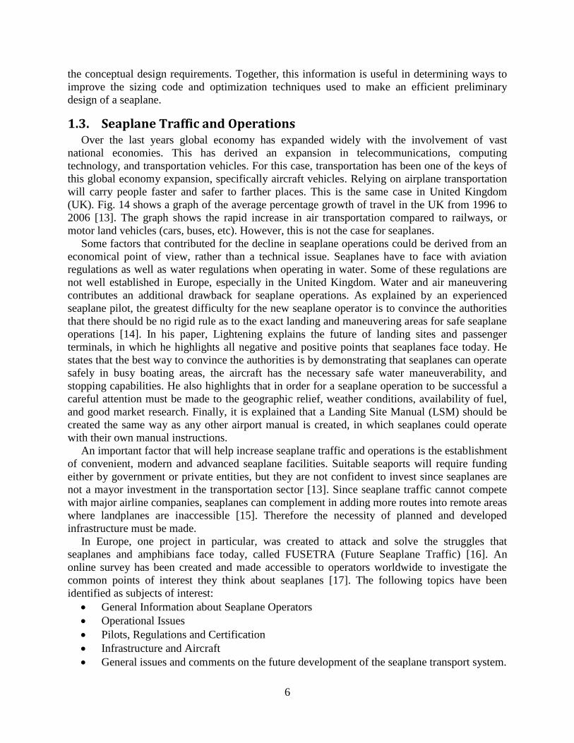
1.3. Seaplane Traffic and Operations Over the last years global economy has expanded widely with the involvement of vast
national economies. This has derived an expansion in telecommunications, computing
technology, and transportation vehicles. For this case, transportation has been one of the keys of
this global economy expansion, specifically aircraft vehicles. Relying on airplane transportation
will carry people faster and safer to farther places. This is the same case in United Kingdom
(UK). Fig. 14 shows a graph of the average percentage growth of travel in the UK from 1996 to
2006 [13]. The graph shows the rapid increase in air transportation compared to railways, or
motor land vehicles (cars, buses, etc). However, this is not the case for seaplanes.
Some factors that contributed for the decline in seaplane operations could be derived from an
economical point of view, rather than a technical issue. Seaplanes have to face with aviation
regulations as well as water regulations when operating in water. Some of these regulations are
not well established in Europe, especially in the United Kingdom. Water and air maneuvering
contributes an additional drawback for seaplane operations. As explained by an experienced
seaplane pilot, the greatest difficulty for the new seaplane operator is to convince the authorities
that there should be no rigid rule as to the exact landing and maneuvering areas for safe seaplane
operations [14]. In his paper, Lightening explains the future of landing sites and passenger
terminals, in which he highlights all negative and positive points that seaplanes face today. He
states that the best way to convince the authorities is by demonstrating that seaplanes can operate
safely in busy boating areas, the aircraft has the necessary safe water maneuverability, and
stopping capabilities. He also highlights that in order for a seaplane operation to be successful a
careful attention must be made to the geographic relief, weather conditions, availability of fuel,
and good market research. Finally, it is explained that a Landing Site Manual (LSM) should be
created the same way as any other airport manual is created, in which seaplanes could operate
with their own manual instructions.
An important factor that will help increase seaplane traffic and operations is the establishment
of convenient, modern and advanced seaplane facilities. Suitable seaports will require funding
either by government or private entities, but they are not confident to invest since seaplanes are
not a mayor investment in the transportation sector [13]. Since seaplane traffic cannot compete
with major airline companies, seaplanes can complement in adding more routes into remote areas
where landplanes are inaccessible [15]. Therefore the necessity of planned and developed
infrastructure must be made.
In Europe, one project in particular, was created to attack and solve the struggles that
seaplanes and amphibians face today, called FUSETRA (Future Seaplane Traffic) [16]. An
online survey has been created and made accessible to operators worldwide to investigate the
common points of interest they think about seaplanes [17]. The following topics have been
identified as subjects of interest:
General Information about Seaplane Operators
Operational Issues
Pilots, Regulations and Certification
Infrastructure and Aircraft
General issues and comments on the future development of the seaplane transport system.

7
Fig. 14: Average Percentage Growth of Travel in the UK [13]
In North America, especially in Canada, the large number of bodies of water and the
remoteness of many important locations has produced an active seaplane traffic. An example is a
seaplane seaport in Vancouver Harbour, Canada shown in Fig. 15. In a concept for the near
future, seaplane facilities are not required to be complex structures where huge amount of
investment must be made. In a simple case, the use of simple mooring buoys and boat, small
beaching ramp, pier or floating docks might fulfill the prerequisites for a seaplane operation
facility.
The current obstacles of social issues, regulations, operations and infrastructure are not in
particularly the only issues confronted. In summary, these were some of the circumstances of the
decline in seaplane operations [16]:
1. Landing on water runways became less ostentatious compared to the increase in the number
and length of land based runways during WWII. 2. WWII left a large amount of landplanes unused and concrete runways on ex-military bases.
Thus, upcoming airlines could purchase this landplanes cheaply from the military. 3. The speed and range of land based aircraft had increased, due to an advance in engine design
and performance. 4. The commercial competitiveness of flying boats diminished, especially since their design
compromised aerodynamic efficiency and speed to accomplish the feat of waterborne takeoff
and landing. 5. Anti-Submarine warfare and Search and Rescue operations could be easily handled by
modern helicopter designs, which give an advantage to operate on smaller ships.
Fig. 15: Seaport in Vancouver Harbor, Canada [15]

8
1.4. Strengths, Weaknesses, Opportunities, and Threats (SWOT) The aim of this SWOT analysis is to recognize the key internal and external factors that are
important to seaplane operations [18]. The SWOT analysis may be then split into two main
categories as follow:
Internal factors: strengths and weaknesses internal to this particular type of transportation.
External factors: opportunities and threats presented by the external environment.
Strengths and weaknesses of seaplane operations are here analyzed under the light of the
“European Aeronautics: a vision for 2020” document [19], where the concept of sustainability is
introduced and made the kernel of the aviation future. EU vision 2020 in not a deadline, but a
sensible reflection on what should lie ahead for Europe in the near future in order to win global
leadership in aeronautics. In vision 2020 aeronautics must satisfy constantly rising demands for
lower costs, better service quality, the highest safety and environmental standards and an air
transport system that is seamlessly integrated with other transport network.
Skies have to be always safer and the most advance automated systems have to be integrated
to eliminate accidents. Aircraft need to be cleaner and quieter and the environment sustainable
with the contribution of the aeronautic sector. The definition of sustainability states that
“sustainability is the concept to endure”. It depends on the wellbeing of the natural world as
whole and the responsible use of natural resources. One EU (European Union) main objective, in
this regard, is to halve, by 2020, carbon dioxide (CO2) emission, perceived noise pollution, and
reduced nitrogen oxide (NOx) emission by 80% from 2000 levels. In conclusion it can be said
that if a generation ago the imperatives were: higher, further and faster, then, according to the
vision 2020 guidelines, these have become: more affordable, safer, cleaner and quieter.
1.4.1. Strengths
One of the major deterrents facing the seaplane market today is the opposition by
environmental authorities on the perceived impact of seaplane. The main argument is based on
the noise impact of seaplane landing, taxiing and taking off, which is known to exceed the
ambient noise level. Additionally, there is a belief that noise, landing and take-off all impact on
wildlife. A current example of this is the on-going dispute between Loch Lomond Seaplanes and
Trossachs National Park. Moreover, as mentioned before, also worldwide the greatest obstacle
facing seaplanes is considered to be the opposition of environmental authorities. In Europe this
was also agreed by 20% of operators [17].
Only few studies have been completed to assess the seaplane environmental impact anywhere
in the world and in many cases these are independent studies carried out by private seaplane
operators [20]. The most inclusive and unbiased is probably an investigation conducted by US
Army corps of Engineers (USACE) [21] and Cronin Millar Consulting Engineers to Harbor Air
Ireland [22], and the outcomes were: No Impact on Air, Water, Soil, Wildlife, Fisheries, and
Hydrology.
It is true that carbon emission generated from seaplane exceed the emission produced by
boats. However, consideration should be given to the fact that the number of boat movements
within any given area greatly outweighs seaplane movements in this area. Additionally, it should
be considered that the next propulsion generation (which is already tested) will have much lower
noise and carbon emission levels. Attention should also be drawn to the fact that seaplanes do
not discharge sewage or oily bilge water and are not treated with toxic anti-fouling paints unlike
boats. Seaplane exhaust are emitted into the air, much above the water giving low water impact,
and currently used seaplane fuel does not contain the flammable and volatile compound MBTE

9
(Methyl Tertiary-Butyl Ether), which is found in boats. Moreover, seaplane propellers are
located away from the water, giving no disturbance on sediments or marine life, and they are
near negligible polluters in regard of foul water and waste from chemical toilettes. Evidently, a
further study validated that floatplanes generate no more than a three inch wake without any
shoreline erosion effects [22].
Seaplanes have relatively low impact on noise pollution too. The majority of noise is
generated during takeoff when high engine power is required to make the seaplane airborne. The
following Table 1 lists typical noise levels for various operations at typical distances from the
sound source and, once again, highlights the minimal impact seaplanes produce.
Attention should be also paid to the fact that the figure quoted is representative of the
seaplane taking off, a short period of daytime-only occurrence which, compared to taxiing and
landing, requires the highest throttle power.
Table 1: Noise levels for various operations [18]
Noise dBA Example
Military jet 120+
Jet ski 110 e.g. watersports on lake
Chainsaw 100-104 e.g. tree felling/ forestry/ logging
Grass Cutting 88-100 Golf courses
Tractors 95 e.g. general operations
All terrain vehicles 85
Speedboat 65-95 e.g. watersports on lake
Seaplane 75 on take-off only @ 300m (20 sec)
Inside car – 30 mph 68-73
Normal conversation 65
In conclusion it may be said that seaplanes do not have negative effect on hydrodynamics,
hydrology, water quality, air quality, wildlife fisheries and birds or noise pollution when
compared to existing background activities on lakes and seaports. Air travel does not develop in
a vacuum: its size, shape and success will be determined by society as a whole. Nowadays there
are specific aspects of air transport that can be better or only satisfied by seaplane/amphibian
operations. The most noticeable strengths in this regard are [18]:
Very versatile type of transportation.
Point to point connections.
Connections to very difficult to reach places.
Safe and efficient surveillance in otherwise inaccessible destinations.
Monitoring of wildlife and management of national parks.
Very good safety records with few incidents during takeoff, landing operations or related to
collisions with boats.
Sightseeing tours/tourism.
Ability to conduct rescue operations over large bodies of water, water bombers.
Avoid the ever congested airfield, holding patterns and control sequences.
No need for runway infrastructures, “unprepared” landing strip, smaller landing fees than
landplanes.
Access from 40% (flying boats) to 70% (amphibian plane) more of the earth’s surface area
than a conventional land plane.

10
1.4.2. Weaknesses
Seaplanes today are “endangered species” and although they posses undoubted potential, the
lack of ability to unlock this potential is due to numerous problems. These are of a various nature
and involve different aspects of seaplane/amphibian’s environment. Certainly, the design aspect
is a major impediment on seaplane advancement and is linked to many other areas. In fact, as
with the introduction of new efficient commercial aircraft designs, the use of the seaplane
declined, no new advanced designs have been made, and most extant seaplanes existing these
days are approaching the end of their operating life. This situation has resulted in a scarcity of
modern and cost-efficient seaplanes. The lack of innovative designs and use of today’s
technology then force seaplanes to VFR (Visual Flight Rules) and make them not suitable in
adverse weather conditions or rough waters. In addition, some environmental issues could, in the
near future, change what is currently a strength factor into a weakness. As stated before, vision
2020 aims to reduce polluting emissions by 50% for CO2 (Carbon dioxide) and by 80%
regarding NOx (Nitrogen oxide). Alternative fuels and new generation engines, together with
better aerodynamic performances, must be considered in order to keep these values as low as
possible and match the suggested targets by the year 2020.
Finally, but equally important, the limited amount of seaplane bases and missing standard
infrastructure equipment is surely a weak point that limits the seaplane market. It means that
refueling and regular maintenance are factors which need serious consideration.
1.4.3. Opportunities
There is huge room for improvements in seaplane operations and many opportunities that can
be exploited in such market. While demand is difficult to forecast without a detailed market
research and an overview of current trends, something that is not available to fledgling
industries, it can be presumed that demand should arise if the industry can offer a different
service from large commercial airlines, either in terms of savings, convenience or novelty.
Following is a list of the main features that may be considered as reliable new opportunities for
seaplane:
Easy usability among places with lots of islands and area/s with (many) resource/s of water.
Faster service compared to ferries when connecting mainland-islands or island-island (e.g.
Greece, UK, Ireland, etc) and the possibility to fly directly from major inland cities catering
also specific groups of commuters in their daily journeys [23].
Unconventional experience from transport (especially for tourists).
Transport with quick dispatching.
To shorten travel times avoiding the use of a combination of other means of transportation
(e.g. Malta-south coast of Sicily) or considerable time savings that can be made where travel
by any land based means is significantly time consuming.
Avionics systems (lighten the burdens on the pilot, help making correct decisions and reduce
human error, night flight). In fact, seaplanes are limited to daytime VFR. Then the way to
eliminate this disadvantage is by adding advance cockpit technology, or the used of advance
gear such as GPS (Global Positioning System), radar, laser altimeters, gyros, advance
sensors, among other gear.
Larger seaplanes with better range, more seats and less affected by weather/water conditions.
Efficient, safe, comfortable infrastructures [24] (seaports, docking facilities, accessibility…).
Air freight services: cargos travel by air because it is more competitive.
11
Modifications of existing planes with innovative new design. Based on the market research
and the technological review, the creation of a new seaplane design will require time,
manufacturing costs, regulation and certification, and social acceptance.
Investments in new technology, materials and new seaplanes/amphibians advance design.
When new advance design is involved, it should be consulted with operators, due to future
equipment plans, and maritime authority regulations should be considered in advance of the
design process. However, it may be expected that new solutions that lower drag when
airborne, maintenance times and costs, and enhance competitiveness in cost/seat/miles ratio
will be always looked forward by operators.
Add value to the air transport market by opening up more locations to air travel and in doing
so make it more convenient, while reducing the congestion on airfields and offering
significant time savings to passengers.
1.4.4. Threats
For seaplanes to really take off there are a number of barriers that must first be overcome.
This paragraph highlights the major threats that seaplane operation is facing today and the
fundamental issues that need to be addressed [14]:
Possibly difficult accessibility of airport (to replace automobile and railway means of
transport is very hard in this case because of difficult approach of airports).
Public perception of light aircraft safety may impact on the acceptability of seaplane
transportation. However, it should be noted that in the UK there has not been a single
reported accident according to their Air Accidents Investigation Branch (AAIB) [25], though
this is in part due to the fact that there have been historically very few seaplane operated in
the UK [26].
Acceptance from population and environmental activists.
Fly time limitations. Alleviation on this regulation is needed so as to better meet the
requirements of seaplane operations thus making them more financially sustainable without
any subsequent of flight safety standards.
Lack of a minimum level of training and acceptability of Dock Operating Crew so as to be
multifunctional with regard to, assisting in the arrival and departure of aircraft on pontoons
or piers, passenger handling, as well as manning the requirements of Rescue and Fire
Fighting activities.
Certification process for new seaplanes.
General regulations: government regulation and control includes both aviation authority
regulations and naval authority regulations. Nowadays there is not a set of unified regulations
throughout Europe and these can also be sometimes in conflict.
Corrosion resistance.
Seaplanes are still too much depended on the weather conditions.

12
2. Literature Review
2.1. Aircraft Design The complexity of aircraft design makes it possible for many proposed methods to be utilized
in order to size an aircraft model. “Sizing” refers to the general size of the aircraft, focusing on
the airplane weight, geometry and other parameters needed to fulfill its required mission
objectives. Raymer [27] has published a detailed breakdown of the steps involved in the
conceptual design of an aircraft. It is explained in detail the processes involved in taking initial
requirements for the aircraft and sizing the aircraft from those requirements. He proposes two
types of sizing processes, Class I and Class II. The Class I sizing process, does a progressive
build-up of the takeoff weight of the aircraft which includes the weight of the crew, payload, fuel
and empty-weight of the aircraft. Based on an empirical ratio of the takeoff weight to the empty
weight of the aircraft, an empty-weight estimation is perform. The ratio depends on the type of
aircraft being designed. The Class II sizing process uses a different method of calculating the
empty weight of the aircraft, in which the individual component weights are calculated based on
statistically weight equations.
The weight process follows a series of steps. First estimates of fuel-fractions (takeoff, climb,
descent, landing, cruise, and reserves) during different portions of the mission are made. Then
the empty weight calculations can proceed. Finally, an iterative approach is used to calculate an
estimated takeoff weight using the estimated fuel-fractions and empty weight equation. An initial
takeoff weight guess is made, followed by the empty weight calculation and an estimate of fuel
fractions, which leads to an estimated takeoff gross weight. Then, the initial guess is compared to
the calculated takeoff gross weight. If the results do not match, a value between the two is used
as a next guess and the process is iterated until convergence is obtained.
Using the initial guess weight, the next step in the sizing process explained by Raymer is to
create the geometry of the aircraft. This includes the selection of an airfoil shape, main wing and
tail geometries, engine and fuselage sizing. Airfoil selection is based on its lift, drag, stall, and
pitching moment characteristics, and available thickness to accommodate ribs and fuel. The main
wing geometry consists of determining the necessary platform area, S, of the wing based on its
gross takeoff weight and lift coefficient. The parameters to determine the wing geometry could
be done by its aspect ratio, taper ratio and sweep and twist angle. The horizontal and vertical tails
are designed using the “tail volume coefficient” method. Engine sizing is performed using
historical thrust-to-weight ratios (T/W) for jet-engine aircraft or power-to-weight ratios for
propeller-powered aircraft. The T/W value is then used to calculate the required lift to drag ratio
during different mission segments. Finally, initial sizing of the fuselage is based on historical
data trend. Raymer’s conceptual design method is based solely on gross takeoff weight but has
shown to have very good correlation to most existing aircraft.
However, as explained before, this research project was mainly focused on the study of the
water operation of the seaplane, rather than the aircraft design. A proposed aircraft design study
had been introduced in order to understand the whole seaplane conceptual design elaborated in
this project. In the end, the seaplane designer can choose whatever design method that is most
suitable and comfortable to elaborate the advance aircraft configuration. This idea can expand
the seaplane designer into converting an existing certified aircraft, i.e. converting an existing
landplane into a seaplane by adding a floating device. The seaplane conversion is cheap to repair
due that it can share all the parts of its landplanes counterparts, except for the floating devices
used.
13
2.1.1. Examples of Existing Landplane for Seaplane Conversion
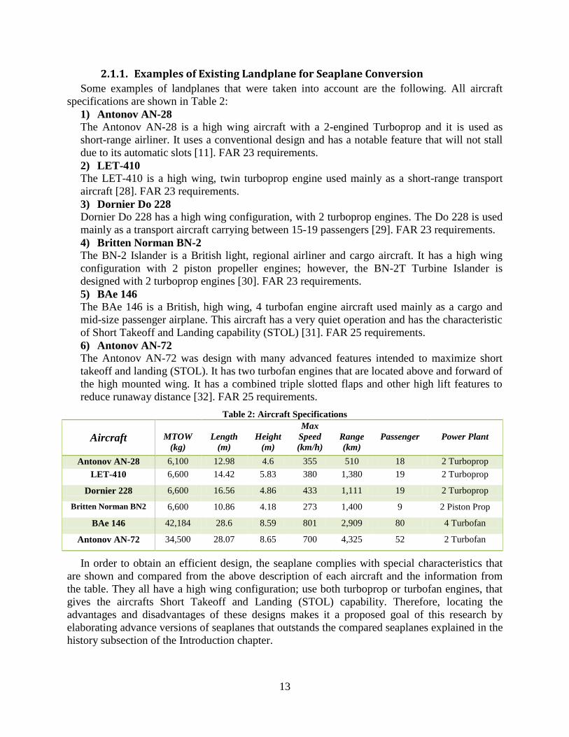
Some examples of landplanes that were taken into account are the following. All aircraft
specifications are shown in Table 2:
1) Antonov AN-28
The Antonov AN-28 is a high wing aircraft with a 2-engined Turboprop and it is used as
short-range airliner. It uses a conventional design and has a notable feature that will not stall
due to its automatic slots [11]. FAR 23 requirements.
2) LET-410
The LET-410 is a high wing, twin turboprop engine used mainly as a short-range transport
aircraft [28]. FAR 23 requirements.
3) Dornier Do 228
Dornier Do 228 has a high wing configuration, with 2 turboprop engines. The Do 228 is used
mainly as a transport aircraft carrying between 15-19 passengers [29]. FAR 23 requirements.
4) Britten Norman BN-2
The BN-2 Islander is a British light, regional airliner and cargo aircraft. It has a high wing
configuration with 2 piston propeller engines; however, the BN-2T Turbine Islander is
designed with 2 turboprop engines [30]. FAR 23 requirements.
5) BAe 146
The BAe 146 is a British, high wing, 4 turbofan engine aircraft used mainly as a cargo and
mid-size passenger airplane. This aircraft has a very quiet operation and has the characteristic
of Short Takeoff and Landing capability (STOL) [31]. FAR 25 requirements.
6) Antonov AN-72
The Antonov AN-72 was design with many advanced features intended to maximize short
takeoff and landing (STOL). It has two turbofan engines that are located above and forward of
the high mounted wing. It has a combined triple slotted flaps and other high lift features to
reduce runaway distance [32]. FAR 25 requirements.
Table 2: Aircraft Specifications
Aircraft
MTOW
(kg)
Length
(m)
Height
(m)
Max
Speed
(km/h)
Range
(km)
Passenger
Power Plant
Antonov AN-28 6,100 12.98 4.6 355 510 18 2 Turboprop
LET-410 6,600 14.42 5.83 380 1,380 19 2 Turboprop
Dornier 228 6,600 16.56 4.86 433 1,111 19 2 Turboprop
Britten Norman BN2 6,600 10.86 4.18 273 1,400 9 2 Piston Prop
BAe 146 42,184 28.6 8.59 801 2,909 80 4 Turbofan
Antonov AN-72 34,500 28.07 8.65 700 4,325 52 2 Turbofan
In order to obtain an efficient design, the seaplane complies with special characteristics that
are shown and compared from the above description of each aircraft and the information from
the table. They all have a high wing configuration; use both turboprop or turbofan engines, that
gives the aircrafts Short Takeoff and Landing (STOL) capability. Therefore, locating the
advantages and disadvantages of these designs makes it a proposed goal of this research by
elaborating advance versions of seaplanes that outstands the compared seaplanes explained in the
history subsection of the Introduction chapter.

14
2.2. Water Operation Design A seaplane is not only to be optimized for aerodynamic, but also for superior hydrodynamic
performance. The drawbacks of a traditional seaplane are [33]:
1. Higher aerodynamic cruise drag due to additional structures.
2. Hydrodynamic drag while planning due to large wetted surface area.
3. Stability issues resulting from limits on dimensions and weight of floating gears.
4. Hindrance from water spray, requiring specially designed shapes to divert the spray away.
5. Low performance in high waves and cross winds, making smooth cruising in rough
weather difficult.
6. Even maneuverability in water could be a deciding criterion, especially where narrow
water strips pose a problem.
Most of the points stated above recall problems associated with the water performance of the
seaplane. The design calls for an extensive investigation in the water operation of a seaplane,
improving the design in such a way that won’t affect other parameters. The extended research
covered an analysis of the old designs looking into the advantages and disadvantages. The design
accounted and implemented the advantages of the old designs, and suggestions for the
disadvantages were researched, until a suitable idea was established.
Let us first recall that the study of the water operation design of a seaplane is focused mainly
on naval architecture terminology, such as beam, step height, fore body, after body, trim angle,
keel angle, stern post angle, etc. A brief explanation of these terms is given.
2.2.1. Hydrodynamic Shape Characteristics
Seaplane hulls and floats share the same shape characteristics that will affect the
hydrodynamic as well as the aerodynamic design. Thus, some of the parameters that largely
affect the hydrodynamic characteristics of the seaplane are shown in Fig. 16.
Fig. 16: Design Features of a Flying Boat [27]
2.2.1.1. Beam Based on the literature review, generally the beam is established as the design reference
parameter of seaplane floats and hull [35]. The beam is the widest section of the float as shown
in Fig. 17.

15
Fig. 17: Beam Width of a Conventional Boat [36]
The beam is determined by the buoyancy requirement and the width required for
accommodation of payload. Loading of a hull is expressed in terms of beam load coefficient
which is based upon the beam as a characteristic dimension and has the following effect on
performance [37]:
· Load to resistance ratio reduces at hump speed with increasing , but increases near
getaway speed.
· Both the upper and lower trim limits of stability are increased.
· Maneuverability decreases and spray increases.
2.2.1.2. Length to Beam ratio The length to beam ratio of a flying boat hull or float is a ratio that affects the drag (either
aerodynamic or hydrodynamic) and resistance of the aircraft. Choosing a slender hull offers
benefits in terms of drag and structural weight. A slender hull is found to carry more weight with
the same resistance than a short or wider hull. As the beam width of the hull increases, the
aerodynamic drag increases. Beam width is related to the cross sectional area and hence the
aerodynamic drag [38]. The length to beam ratio is directly linked to structural weight. The
structural weight tends to increase with the product of length and beam.
For length to beam ratios between 9 and 10, no gain in hydrodynamic characteristics is
obtained. Hulls with length to beam ratios between 6.3 and 9, the stability range of center of
gravity locations are the same [37].
2.2.1.3. Forebody and Afterbody Length A seaplane can be divided into forebody and afterbody depending upon the location of the
step. The location of the step however has to be optimized, assuming the aspect ratio to be
constant, so as to derive favorable hydrodynamic characteristics. Another assumption made is
that the center of gravity remains or fixed relative to the step in order to eliminate inherent
changes in trim.
2.2.1.4. Deadrise Angle Deadrise is the angle of the bottom of the hull in a cross-section view of a boat. Angles of
deadrise ranging from 20 degrees to 30 degrees probably represent the best overall performance
suggested by World War II designs. Tank tests on the effect of deadrise angles were done on
hulls of the Sunderland III [39]:
· Increasing the deadrise in the range of 15 to 30 degrees has little effect on hump resistance.
· Resistance increases at speeds exceeding the hump speed.
· The positive trimming moment at planning speed increases.
· The lower trim limit of stability increases with deadrise angle.
· Impact loads are considerably reduced.

16
Another study indicated that landing stability is improved by increasing the deadrise from 20
to 25 degrees [40]. Further studies confirm the most noticeably effect of deadrise angle is on
impact loads which goes down with increasing deadrise angle [38].
However, increasing the dead rise angle at step makes the hull bottom a less efficient planning
device. The hull will ride more deeply in water and hence will experience increased frictional
drag an effect more pronounced in the planning range.
2.2.1.5. Hull Bottom Fig. 18 shows a variety of different bottom shapes for a boat hull or float aircraft. The bottom
chosen will always be a compromise between quick takeoff and seaworthiness. According to
Brimm [41], the flatter the bottom, the quicker an aircraft will takeoff in calm seas. But, in
rougher seas, the flatter bottom will cause severe pounding due to wave slam, which will likely
make the aircraft takeoff slower than if it had a sharp bottom, which cuts through waves instead
of going over them. This tendency to slam in rough water makes having a flat bottom hull a poor
choice for an amphibious aircraft that is to operate in the littoral zone.
The double concave is desirable because it combines the advantages of the sharp and blunt
“Vee”. It has a sharp edge for entry into the water and cutting through waves yet still has a
comparatively flat surface on which to plane. Another benefit of the double concave is that it
deflects spray down and away from the fuselage and wings of the aircraft, which decreases loads
and reduces the threat of water spray into the engines. The best overall compromise is the double
scalloped bottom. Not only does it share the advantages of the double concave, but as the aircraft
increases speed and begins to plane, it begins to rise up out of the water, and is supported on
successively lower scallops, reducing the water resistance as the speed increases. The forebody
of the boat hull was chosen to have a double scalloped bottom, for its combination of reduced
drag and spray characteristics as well as its ability to cut through the water, while the afterbody
was designed to be a double concave because of its behavior during planning.
Fig. 18: Various Types of Boat Hull Bottoms [41]
2.2.1.6. Step When water moves over the convex surface of the bottom of a seaplane, it creates suction in a
normal direction to the surface. This means that as an amphibious aircraft accelerates through the
water, the downward suction would increase with increasing speed. Takeoff performance would
be greatly hampered by this. To prevent this from happening, a sharp step is placed into the hull
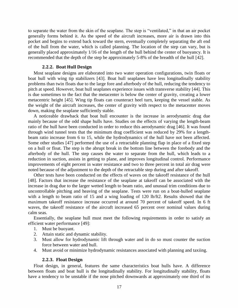
17
to separate the water from the skin of the seaplane. The step is “ventilated,” in that an air pocket
generally forms behind it. As the speed of the aircraft increases, more air is drawn into this
pocket and begins to extend back toward the stern, eventually completely separating the aft end
of the hull from the water, which is called planning. The location of the step can vary, but is
generally placed approximately 1/16 of the length of the hull behind the center of buoyancy. It is
recommended that the depth of the step be approximately 5-8% of the breadth of the hull [42].
2.2.2. Boat Hull Design
Most seaplane designs are elaborated into two water operation configurations, twin floats or
boat hull with wing tip stabilizers [43]. Boat hull seaplanes have less longitudinally stability
problems than twin floats due to the large fore and afterbody of the hull, reducing the tendency to
pitch at speed. However, boat hull seaplanes experience issues with transverse stability [44]. This
is due sometimes to the fact that the metacenter is below the center of gravity, creating a lower
metacentric height [45]. Wing tip floats can counteract heel turn, keeping the vessel stable. As
the weight of the aircraft increases, the center of gravity with respect to the metacenter moves
down, making the seaplane sufficiently stable.
A noticeable drawback that boat hull encounter is the increase in aerodynamic drag due
mainly because of the odd shape hulls have. Studies on the effects of varying the length-beam
ratio of the hull have been conducted in order to reduce this aerodynamic drag [46]. It was found
through wind tunnel tests that the minimum drag coefficient was reduced by 29% for a length-
beam ratio increase from 6 to 15, while the hydrodynamics of the hull have not been affected.
Some other studies [47] performed the use of a retractable planning flap in place of a fixed step
on a hull or float. The step is the abrupt break in the bottom line between the forebody and the
afterbody of the hull. The step causes the water to separate from the hull, which leads to a
reduction in suction, assists in getting to plane, and improves longitudinal control. Performance
improvements of eight percent in water resistance and two to three percent in total air drag were
noted because of the adjustment to the depth of the retractable step during and after takeoff.
Other tests have been conducted on the effects of waves on the takeoff resistance of the hull
[48]. Factors that increase the resistance of the seaplane at takeoff can be associated with the
increase in drag due to the larger wetted length to beam ratio, and unusual trim conditions due to
uncontrollable pitching and heaving of the seaplane. Tests were run on a boat-hulled seaplane
with a length to beam ratio of 15 and a wing loading of 120 lb/ft2. Results showed that the
maximum takeoff resistance increase occurred at around 70 percent of takeoff speed. In 6 ft
waves, the takeoff resistance of the aircraft increased 65 percent over nominal values during
calm seas.
Essentially, the seaplane hull must meet the following requirements in order to satisfy an
efficient water performance [49]:
1. Must be buoyant.
2. Attain static and dynamic stability.
3. Must allow for hydrodynamic lift through water and in do so must counter the suction
force between water and hull.
4. Must avoid or minimize hydrodynamic resistances associated with planning and taxiing.
2.2.3. Float Design
Float design, in general, features the same characteristics boat hulls have. A difference
between floats and boat hull is the longitudinally stability. For longitudinally stability, floats
have a tendency to be unstable if the nose pitched downwards at approximately one third of its

18
takeoff speed. The region of greatest curvature, which is generally towards the front of the float,
shows suction over the bottom that causes the longitudinal instability. Though, if the float could
be longitudinally stable by restoring the moment, it would still be susceptible to instability
caused due to insufficient damping, which results in oscillations known as porpoising [50].
Porpoising is a dynamic instability of the seaplane and may occur when the seaplane is
moving across the water while on the step during takeoff or landing [51]. It occurs when the
angle between the float or hull, and the water surface exceeds the upper or lower limit of the
seaplane's pitch angle. There are two types of porpoising. One type can be counteracted by
applying a steady load to the horizontal tail surface, which causes the aircraft to pass to another
trim angle, “getting through” the porpoising as quickly as possible. The second type can only be
counteracted through an alternative application of upward and downward loads on the tail
surfaces, although even this is not always successful.
2.2.4. Trimaran and Retractable Float System
Many proposed ideas were analyzed for possible technical solutions that aim to reduce costs
on research, manufacturing and operation of the advance seaplane design. Some water operation
ideas that were considered were the use of retractable floats, inflatable floats, advance
navigational aid instruments, hydrofoils, water thrusters, folded wings, advance composite
materials, reversed thrusters, multihulls, among many more ideas.
Inflatable floats will give the advantage of reducing aerodynamic drag; however the main
concern of inflatable floats will be stability and control of the seaplane during water operations.
Water thrusters can be used to aid the seaplane maneuvering in water when taxiing in the
seaport, but water thrusters may increase payload weight and they will become useless once the
seaplane is in the air. Retractable wings can be used when the seaplane is operating on water to
reduce clearance space and have a better access to seaports and maintenance hubs. Navigation
aid instruments will be useful for a seaplane to operate in many types of weather conditions.
Hydrofoil, shown in Fig. 19, is a foil that operates on water. A hydrofoil is a wing-like structure
mounted on the bottom or side of a boat hull and its purpose is to lift the boat out of the water in
order to reduce hull water resistance [52].
After analyzing all of the proposed ideas, the complexity and high costs of some of these
narrow the search for technical solutions that will meet the requirements of this futuristic
seaplane concept. It was decided that the use of trimaran hull and the use of retractable floats will
give the seaplane an exceptional performance.
Fig. 19: Hydrofoil Example [53]
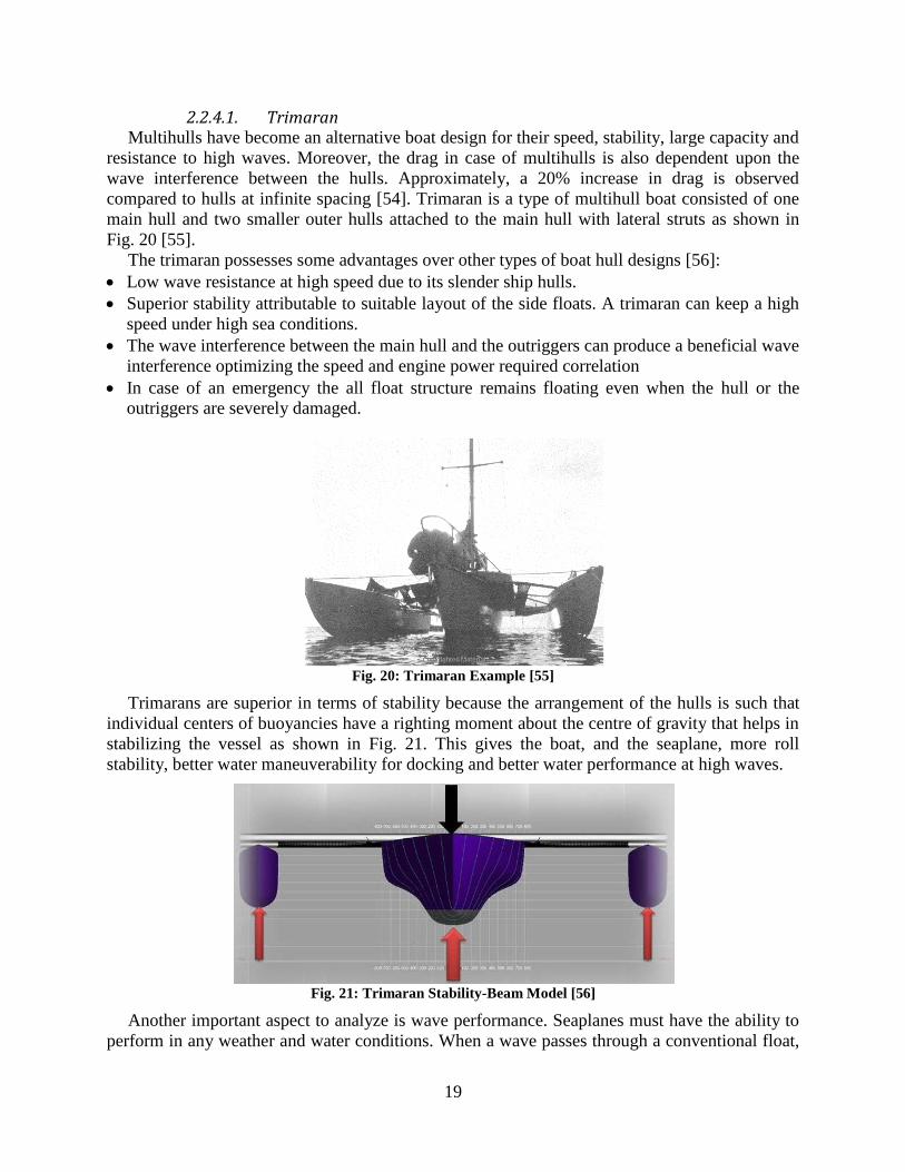
19
2.2.4.1. Trimaran Multihulls have become an alternative boat design for their speed, stability, large capacity and
resistance to high waves. Moreover, the drag in case of multihulls is also dependent upon the
wave interference between the hulls. Approximately, a 20% increase in drag is observed
compared to hulls at infinite spacing [54]. Trimaran is a type of multihull boat consisted of one
main hull and two smaller outer hulls attached to the main hull with lateral struts as shown in
Fig. 20 [55].
The trimaran possesses some advantages over other types of boat hull designs [56]:
Low wave resistance at high speed due to its slender ship hulls.
Superior stability attributable to suitable layout of the side floats. A trimaran can keep a high
speed under high sea conditions.
The wave interference between the main hull and the outriggers can produce a beneficial wave
interference optimizing the speed and engine power required correlation
In case of an emergency the all float structure remains floating even when the hull or the
outriggers are severely damaged.
Fig. 20: Trimaran Example [55]
Trimarans are superior in terms of stability because the arrangement of the hulls is such that
individual centers of buoyancies have a righting moment about the centre of gravity that helps in
stabilizing the vessel as shown in Fig. 21. This gives the boat, and the seaplane, more roll
stability, better water maneuverability for docking and better water performance at high waves.
Fig. 21: Trimaran Stability-Beam Model [56]
Another important aspect to analyze is wave performance. Seaplanes must have the ability to
perform in any weather and water conditions. When a wave passes through a conventional float,

20
it reaches the bow producing a lift force which pushes the stern down; as the wave passes
through the body of the float, the center of buoyancy changes along with the wave. When the
wave reaches the stern, the lift force pushes the bow; at high speeds, during rough water
conditions, a dangerous pitch effect could cause the bow to be submerged and capsize violently.
For the outriggers, when the peak of the wave moves towards stern, the lack of buoyancy on this
section to the shape, negates the lift force which produces the pitching effect, therefore the
outriggers are capable to operate in a wider range of rough water conditions than the
conventional floats. Past studies conducted on trimaran shows that wave resistance of trimarans
is significantly lower compared to an equivalent catamaran as shown in Fig. 22 [57]. For this
instance, in theory, trimaran has superior seagoing performance.
Fig. 22: Resistance comparison curves [57]
2.2.4.2. Outrigger Design The total resistance of the trimaran can be reduced by the design of the outrigger form and
position. For an ideal trimaran design, an outrigger is half the length of the main hull and has 4%
of the displacement of the main hull [58]. The positions of the outriggers with respect to the main
hull are quantified in terms of the longitudinal displacement of the centre line of the outrigger
from then centerline of the hull (known as clearance) and the lateral displacement of the
outrigger with respect to the main hull (known as stagger), shown in the following figures.
Fig. 23: Trimaran coordinate Axis [56]
1 1.5 2 2.5 3 3.50.5
1
1.5
2x 10
4
Froude Number
Resis
tance [
N]
Total Resistance Values
Monohull
Catamaran
Trimaran

21
Fig. 24: Outrigger stagger and clearance [56]
Assuming that the mid latitude of the main hull is the origin of the coordinate system, positive
stagger is the distance of the mid latitude of the outrigger in the direction of the stern. Clearance
is the departure of the centerline of the outrigger from the centerline of the main hull in the
vertical direction.
The stagger ‘x’ and the clearance ‘y’ are rendered dimensionless by representing them as a
ratio to the total length of the main hull. The following results performed by Begovic [58] of tank
tests done for a series 64 trimaran hull with different stagger and clearance. The first series of
tests involved testing the model for a stagger ‘x/L’ = -0.0625 and for clearances of 0.10, 0.11 and
0.12 respectively. The second series involved testing the model for a clearance ‘y/L’ = 0.1 and
staggers of 0.25, 0, -0.0625 and -0.125 respectively.
For the tested clearance 0.10, minimum resistance was obtained for a stagger of - 0.125 in the
Froude number range of 0.7 to 1.0, probably due resulting from a larger lift effect. However this
layout is fairly unrealistic for large scale trimarans. Therefore, the results of the two practical
values of stagger (the values of 0 and -0.0625) were considered. It was also observed that
resistance dropped further with the clearance due to changes in the interference phenomenon.
2.2.4.3. Retractable Float System One concern of using trimaran will be the exposed floats at flight. One solution is to retract
the floats or either mount them inside the fuselage or hull, which in theory reduces aerodynamic
drag.
Tigerfish Aviation developed the use of retractable pontoons called Retractable Amphibious
Pontoon Technology (RAPT) [59]. Adapting the same concept idea, the floats will form a single
component embodied to the hull and fuselage when retracted, as shown in Fig. 25. This will
reduce the drag form interference factor added by the floats and boat hull [60], hence decreasing
the aerodynamic drag. However, retracting the floats into this position will not reduce entirely
the aerodynamic drag caused by the floats. A final solution is to place the floats inside the boat
hull, as shown in Fig. 26. The floats will be retracted inside the boat hull, the same way the
landing gear is retracted inside the fuselage. The only drawback will be the added structural
support required, compromising an increase in weight of the strutting.
For this design, another advantage of the retracting float system was to keep the seaplane
stable. The retracting system can be automated in order to control the seaplane on unexpected
heel turns. If the seaplane tilts to a side, the automated retracting system will be configure to
maintain a position in the water in which one float will move upwards towards the waterline
while the other float will move downwards, maintaining both floats at the waterline. Fig. 27
shows the mechanism of the retracting system in the water.

22
Last, another advantage of the floats will be as an extra storage compartment. Since the floats
do not account for the total displacement of the seaplane, extra fuel or payload could be stored
inside the floats, increasing the performance of the seaplane.
Fig. 25: Retracting Float Concept [59]
Fig. 26: Example CAD Model with Floats retracted inside Hull
Fig. 27: Heel Overturn Retracting Float System

23
3. Advance Seaplane Conceptual Optimization Method
3.1. Conceptual Design The first step of this research was the creation of an advanced seaplane conceptual design
method. Many old seaplane publications approached the conceptual design by developing the
water operation requirements (i.e. the boat hull or floats) before the air requirements [35], [42],
[44]. With the hull sized, the fuselage of the aircraft was built around the hull dimensions, and
the rest of the aircraft components (wings, empennage, etc.) were then added. In other words,
seaplane design had to comply with water requirements before fulfilling air requirements. The
design must perform an acceptable hydrostatic stability, with outstanding aerodynamic and
hydrodynamic properties, and a strong structure supporting water loads. This gives the seaplane
designer a disadvantage in having an open mind on the manner on how to elaborate an advance
seaplane design with an “out of the box” aircraft configuration.
Nonetheless, the idea to create a modern conceptual design that will allow the designer to
create a futuristic seaplane, made it possible for this research to analyze the proposed method.
The advance seaplane design method was elaborated by gathering studied seaplane information,
adapting the advantages of the old seaplane features, and attacking the disadvantages in order to
modify them by creating the modern conceptual seaplane design.
To generalize, the proposed design sizes each of the seaplane segments (“boat” and “aircraft”)
in a separate manner. There are three main advantages of adapting this conceptual design:
1. The “aircraft” segment can be design in a separate manner, using whatever optimization
method the designer will like to choose. The “boat” optimization design method was
elaborated in such a manner that will adapt which ever aircraft configuration and will then
design the desire water operation device design parameters. Therefore,
2. The conversion of an existing landplane structure into a seaplane configuration will be
elaborated into this design method.
3. Simplification of this method will expand the complexity of creating an advance seaplane
“boat” segment by studying a more reliable hull design and running separate trial tests.
Since the design of an aircraft has to comply with many requirements such as airworthiness,
stability, structural strength, etc., only certain requirements of the seaplane were analyzed for
simplicity of this research. Air stability, structural strength, and engine modeling were not
analyzed in this research. For this instance, to recognize which aspects to study, the research
attacks the most noticeable disadvantages common seaplane designs have today. This way,
seaplanes will have excellent air performance as well as water performance to compete in the
global aeronautical industry. Then, the main goals that should be attained to acquire the desire
design were focused on the following:
1. The seaplane should acquire an outstanding hydrostatic stability in order to excel during
water taxing operations, hence the trimaran concept.
2. The advance design will have the capability to operate in rough, high wave waters, giving
the seaplane more water options in which to operate.
3. The increase in aerodynamic drag caused by the extra components should not compromise
the flight performance of the seaplane, hence the retracting float system.
4. Water Performance should be comparable to that of a speed boat.
5. Air Performance must obtain related performance as that to its landplane design.
Then, in order to attain the necessary criteria explained, the advance design follows the
proposed flow chart shown in Fig. 28.
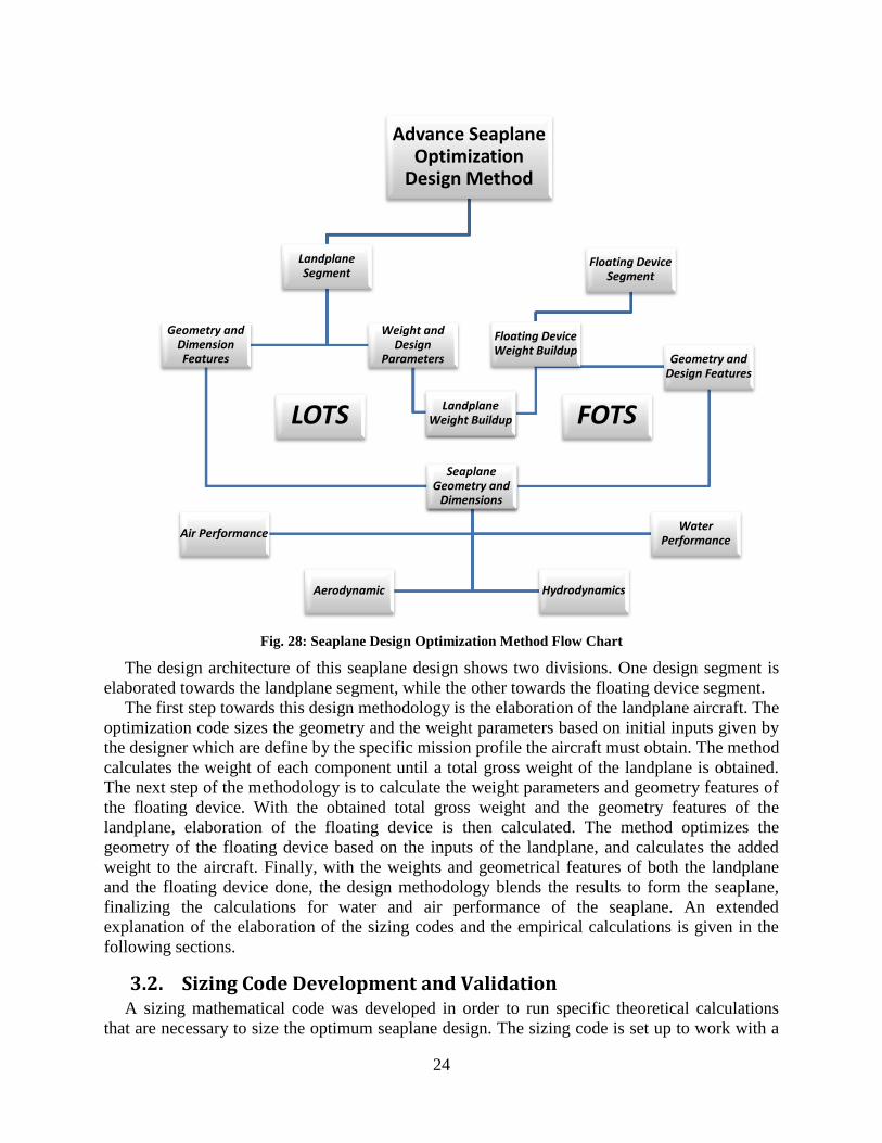
24
Fig. 28: Seaplane Design Optimization Method Flow Chart
The design architecture of this seaplane design shows two divisions. One design segment is
elaborated towards the landplane segment, while the other towards the floating device segment.
The first step towards this design methodology is the elaboration of the landplane aircraft. The
optimization code sizes the geometry and the weight parameters based on initial inputs given by
the designer which are define by the specific mission profile the aircraft must obtain. The method
calculates the weight of each component until a total gross weight of the landplane is obtained.
The next step of the methodology is to calculate the weight parameters and geometry features of
the floating device. With the obtained total gross weight and the geometry features of the
landplane, elaboration of the floating device is then calculated. The method optimizes the
geometry of the floating device based on the inputs of the landplane, and calculates the added
weight to the aircraft. Finally, with the weights and geometrical features of both the landplane
and the floating device done, the design methodology blends the results to form the seaplane,
finalizing the calculations for water and air performance of the seaplane. An extended
explanation of the elaboration of the sizing codes and the empirical calculations is given in the
following sections.
3.2. Sizing Code Development and Validation A sizing mathematical code was developed in order to run specific theoretical calculations
that are necessary to size the optimum seaplane design. The sizing code is set up to work with a
Advance Seaplane Optimization
Design Method
Landplane Segment
Geometry and Dimension Features
Air Performance Water
Performance
Hydrodynamics Aerodynamic
Weight and Design
Parameters
Landplane Weight Buildup
Floating Device Segment
Floating Device Weight Buildup
Landplane Weight Buildup
Geometry and Design Features
Seaplane Geometry and
Dimensions
LOTS FOTS
25
number of different aircraft configurations which would then add the desired floating device
(boat hull, twin floats, wing tip floats, trimaran) to transform the landplane aircraft into an
amphibious configuration. To increase the usefulness of the sizing code, as well as to obtain a
more feasible final preliminary design, any combination of the various water operations methods
may be used, which allows for testing as many configurations as possible.
The seaplane optimization code works in two separate optimization codes. The first code
called the Landplane Optimized Testing Source Code or LOTS, sizes the characteristics of the
landplane aircraft chosen. The second code, called the Floating Device Optimized Testing
Source Code or FOTS, sizes the floating device chosen by the seaplane designer, based on the
characteristics given by the landplane.
3.2.1. Landplane Optimized Testing Source Code (LOTS)
Using Raymer’s Class II sizing process design method the following Landplane Optimized
Testing Source Code (LOTS) was elaborated. The LOTS code was written using the Mathwork’s
MATLAB programming language and compiler. Separate functions were written to accomplish
various tasks, which are all then compiled into pre-processing, computation and post-processing
codes. The following image (Fig. 29) shows the proposed flowchart of the LOTS architecture.
To begin the optimization sizing code, selection of desired input parameters must be made by the
designer depending on the mission requirements the aircraft must perform. These parameters are
wing aspect ratio (AR), Wing Loading (W/S), taper ratio (λ), and tail volume coefficients. Then,
an initial guess for GW is made and aircraft geometry, such as wing span and wing area, are
calculated. Using these values, weights of individual components are calculated and summed
together to get a GW. The two GWs are compared and iterated until convergence. Depending on
the mission requirements, then the mission code is run, which calls upon the various other cruise
codes, in order to get a weight of the fuel required for the mission. Once this is obtained, new
aircraft geometries are calculated and both the weights and mission codes are run until a GW is
converged. Then, the drag code is ran which calculates a more accurate at plat drag based on the
current aircraft geometry and weight. Once this value is obtained, the drag code is iterated with
the weights and mission code until a common GW and equivalent at plate drag value is obtained.
Once these values are converged, the program calls upon the final process in order to determine
if this aircraft meets the mission requirements. If the requirements are met, then the data is saved
as a comma separated value file. If the requirements are not met, then the values are deleted and
new values for AR and/or W/S are run.
As explained before, LOTS is able to size three different aircraft configurations, conventional,
BWB, and Flying Wing. Let us recall that this research project does not emphasis the work of the
optimizer source code, so a depth explanation is not elaborated. Principle algorithms and
numerical iteration methods are run throughout the code in order to size the landplane geometry
and flying characteristics. As stated, the designer may be eligible to use any computation device
or code to elaborate the desire aircraft design.

26
Fig. 29: Flowchart of the LOTS architecture
3.2.2. Floating Device Optimized Testing Source Code (FOTS)
The Floating Device Optimized Testing Source Code (FOTS) functions similarly as the LOTS
sizing code. The proposed flowchart architecture of the FOTS code is shown in Fig. 30.
The FOTS sizing code will start by entering the output characteristics of the landplane sized
by the LOTS code. Fig. 31 shows the input characteristics of the landplane necessary to calculate
the floating device characteristics. Based on the input gross weight of the landplane, the FOTS
code calculates the buoyancy required which is necessary to size the dimensions of the floating
device. The designer chooses either a boat hull with mid wing stabilizers, boat hull with wing tip
floats, twin floats, or boat hull with twin floats (trimaran). The designer then chooses a
slenderness ratio and a spray coefficient depending on the characteristics of the seaplane desired
by the designer. With the buoyancy calculated, and the slenderness ratio and spray coefficient
chosen, the code sizes the dimensions of the main hull. The code then checks if the length of the
fuselage is less or equal to the length of the boat hull. If this is the case, the code continues to
size the rest of the floating device. If this is not the case, the code selects new slenderness ratio
and spray coefficient until it converges to the desire hull length value. With the hull and the rest
of the floating device sized (stabilizers) the code checks for hydrostatic stability requirements. If
the hydrostatic stability is not met, the code runs new values of slenderness ratio and spray
coefficients running the geometric loop again. When hydrostatic stability is satisfied, water
takeoff is calculated based on the thrust available (TA) of the landplane. If the water takeoff is not
satisfied, either a new TA is needed from the LOTS code, resizing the whole landplane
parameters, and starting the sizing methodology, or the FOTS code changes the geometry of the
floating device which will be resized until convergence. When all requirements are met, the
seaplane features are given, and geometry and performance characteristics are then output. With
this data obtained, a picture showing the basic geometry is drawn.

27
Fig. 30: Flowchart of FOTS architecture
Fig. 31: Input Landplane Characteristics

28
3.2.3. Validation
In order to validate the functionality of the sizing code and to ensure that the sizing algorithms
used in the code are working properly over a range of aircraft types, geometry of an aircraft was
run through the code to determine how the coded algorithms predicted the takeoff weight and
performance parameters. First, validation of the LOTS sizing code was done by comparing data
from the LET L-140 [28]. For simplicity, the validation assumed no floating device was added;
therefore the FOTS sizing code calculated the air performance of the landplane. The following
comparison data obtained from the sizing code is shown in Table 3.
Table 3: LOTS Comparison Validation
Parameters Typical Let L-410 % Error
Gross Weight [kg] 6,600 6,670 1.05%
Empty Weight [kg] 3,900 4,020 2.99%
Max Fuel [kg] 1,300 1,370 5.11%
Fuselage Length [m] 14.47 14.43 0.28%
Wing Area [m2] 34.86 34.9 0.11%
Wing Span [m] 19.08 19.7 3.15%
Max Speed [km/hr] 392 390 0.51%
Rate of Climb [m/s] 6.6 7 5.71%
Service Ceiling [km] 7.27 7.4 1.76%
Thrust Available [N] 25,500 25,000 2.00%
Now validation of the FOTS sizing code was done by comparing the performance of the
Canadair CL-215 amphibian aircraft [11]. In this case, the LOTS sizing code sized the aircraft
without the floating device. Then the FOTS sizing code adds the boat hull and stabilizer floats,
and finally the performance was calculated. This validation is only an approximation on the
functionality of the sizing codes and not necessarily sizes the aircraft from the original sample.
Table 4 shows the comparison data of the Canadair CL-215.
Table 4: FOTS Comparison Validation
Input Typical Canadair % Error
Gross Weight [kg] 17,000 17,100 0.58%
Empty Weight [kg] 12,000 12,200 1.64%
Max Fuel [kg] 3,800 3,800 0.00%
Fuselage Length [m] 21.2 19.82 6.96%
Wing Area [m2] 98.52 100.3 1.77%
Wing Span [m] 26.5 28.6 7.34%
Max Speed [km/hr] 396 360 10.00%
Rate of Climb [m/s] 9.2 8.1 13.58%
Service Ceiling [km] 5.2 4.5 15.56%
Thrust Available [N] 67,000 67,500 0.74%
The data obtained shows the functionality of the advance seaplane sizing code. The LOTS
code has a percent of error of less than 5% over most of the parameters compared, proving a
good functionality of the algorithms. On the other hand, the FOTS code shows a percent error of
29
less than 15% in some parameters. The reason for increase in percent error is the newly air
performance calculation done when the floating device is added to the landplane. As explained,
the sizing methodology proposed differs from the conventional seaplane conceptual designs.
3.3. Theory The seaplane conceptual design and the sizing code followed a proposed aircraft design
theory in order to size the optimum advance amphibian aircraft. Basic aircraft design theory
proposed by Raymer was used [27]. Water performance theory was elaborated with the aid of
many proposed publications [35],[38],[42],[44],[45] and finally adapting the use of the trimaran
design blended with conventional flying boat theory [57].
3.3.1. Aeronautical Theory
Since the study of aircraft design has been elaborated for many years, this field of study has
been corrected and improved in order to find suitable empirical equations that will size the desire
aircraft design. As explained previously, the seaplane designer can use the optimization process
desired and in this case, the theoretical calculations necessary to size the landplane aircraft. For
the purpose of this research, only a brief explanation of landplane aircraft theory is given. The
sizing theory of the landplane aircraft follows the flowchart architecture shown from Fig. 29.
3.3.1.1. Geometry Calculations The first step of the LOTS code is to size the major components of the aircraft based on the
initial parameters (GW, AR, W/S, λ, etc.). The required platform area of the main wing, S, can be
calculated using the estimated gross takeoff weight and wing loading.
⁄ ( 1 )
The total wing span of the main wing can be found using eq. ( 2 )
√ ( 2 )
The root and tip chord lengths are calculated using the following expressions:
( ) ( 3 )
( 4 )
The platform areas for the vertical and horizontal tails are calculated using the following
equations from Raymer [27].
( 5 )
( 6 )

30
3.3.1.2. Weights The first step in calculating the weight of an aircraft is to identify the “Design takeoff gross
weight (GW)” [27]. Takeoff gross weight can be divided into payload weight, fuel weight, and
empty weight as shown from the following equation.
( 7 )
Payload weight and fuel weight would be determined depending on the mission requirements
of the aircraft, such as amount of passengers or cargo, the range or endurance, among other
characteristics.
3.3.1.2.1. Empty Weight With the geometry of the aircraft found, an empty weight breakdown of each component of
the aircraft is calculated. Empty Weight breakdown is elaborated using the statistical equations
proposed by Raymer [61] and shown in Appendix A.1. All equations and multiplicative factors
are taken for a general aviation aircraft, unless specified.
3.3.1.2.2. Fuel Weight Total fuel weight is broken down into each of the required segments the aircraft needs to
perform in order to attain its mission, take-off, climb, cruise, descent, and landing, as well
accounting for taxi operations and reserves. Then the equation for fuel weight is:
( 8 )
Where L is level flight, Taxi is fuel at taxi segment, TO stands for take-off, C is climb, D is
for descent, LN is for landing, and H is for holding fuel or fuel reserve. To calculate the mass of
the fuel for each segment the following equation is used:
( 9 )
Fuel consumption (FC) depends on the available thrust and thrust specific fuel consumption
which is explained in more detail in the engine modeling section.
3.3.1.3. Aerodynamic Drag
Drag forces results from a combination of pressure and shear forces. Alternatively, the drag
forces are broken down into induced drag and wave drag which is the drag due to pressure forces
and viscous or parasite drag which accounts for the shear forces.
( 10 )
3.3.1.3.1. Induced Drag The vortices caused by the wing in generating lift also cause the effective angle of attack of
the wing to be lowered. This phenomenon slightly reduces lift but causes a noticeable increase in
drag. The drag that is created by this phenomenon is known as induced drag. Induced drag
greatly depends on the lift distribution of the wing, with an elliptical wing loading being the most
efficient with the lowest amount of induced drag [60].
The total induced drag coefficient is then found using the equation,
( 11 )

31
To relate a given wing distribution to an elliptical wing distribution, the Oswald efficiency
factor (e) is calculated from Raymer [60].
Straight Wing ( ) ( 12 )
Swept Wing ( )( ) ( 13 )
3.3.1.3.2. Wave Drag In high subsonic flight, regions on the wing can experience air speeds of over Mach 1. This
will in turn cause shock waves to form which cause adverse pressure distributions that increase
the drag of the wing. This is known as wave drag. Wave drag is calculated by finding the Mach
number at which the wing experiences supersonic flows, also known as divergence Mach
number (Mdiv). Mdiv is greatly influenced by wing sweep ( ), CL and wing thickness ratio (t/c).
Higher increases Mdiv, while a larger CL and t/c decreases Mdiv. According to [63], a plane with
a of 35o and a t/c of 10%, the minimum Mdiv number is 0.79. Wave drag is calculated using the
method provided by [63].
( ) ( 14 )
( ) ( 15 )
3.3.1.3.3. Parasite Drag Surface tension effects create a force opposing the relative motion of aircraft as particles of air
move over the exposed surfaces, or wetted area. This is known as friction or parasitic drag and is
the major contribution to drag in low speed flight. A useful measure of the parasite drag is the
equivalent flat plate-drag area (f). Therefore, the total parasite drag (DP) is [27], [68]:
( 16 )
Each exterior component of the airplane is considered separately, and the total (f) of each
component is finally sum together. The equivalent flat plate drag area can be computed from the
following expression:
( 17 )
Where (Cf) is coefficient of friction, (F) is form factor, (Q) is interference factor and (Swet) is
the wetted area of the component. These variables are calculated using the equations from
Appendix A.2.
Miscellaneous component flat plate area is an additional 5% increase to the flat plate drag to
take into account of sensors, joints, and other surface disturbances. The total parasitic drag
coefficient is then found using,
( 18 )
3.3.1.4. Air Performance “Performance” is a term used to describe the ability of an airplane to accomplish certain
things that make it useful for certain purposes. For example, the ability of the airplane to land

32
and take off in a very short distance is an important factor to the pilot who operates in and out of
short, unimproved airfields. The ability to carry heavy loads, fly at high altitudes at fast speeds,
or travel long distances is essential performance for operators of airline and executive type
airplanes. The chief elements of performance are the takeoff and landing distance, rate of climb,
ceiling, payload, range, speed, manoeuvrability, stability, and fuel economy. For simplicity and
the complexity of the subjects, manoeuvrability and stability are concepts that were not widely
researched. Then, basic fundamental equations for calculating the performance of the aircraft
were done with the aid from several handouts [28]. Some of the key equations for the calculation
of the performance are shown in this section while the rest are in Appendix A.3.
One of the most important graphs in aircraft performance is thrust as a function of velocity. A
comparison of the required thrust and power calculations are given by using the following
equations:
( 19 )
Some important speed performance parameters are stall speed (VS0), climb speed (Vc), which
are calculated by the following:
√
( 20 )
( )
( 21 )
Last, other important parameters useful in the performance of an aircraft are endurance and
range. Using Breguet Range equation, endurance and range are calculated:
(
) ( 22 )
( 23 )
3.3.1.5. Engine Modeling To calculate the weight of the fuel for each flight segment of the aircraft, it is necessary to
calculate the amount of fuel consumption the engines produced. Then, from the following:
( 24 )
i represents the flight segment (takeoff, descent, etc.) An equation for the fuel flow can be
found based upon the thrust of the engine. The referred fuel flow is the engine fuel flow
normalized by the pressure and temperature ratios and the engine thrust is normalized by the
pressure ratio. Therefore, the equation for fuel flow (tsfc) is:
( )√ ( 25 )
Engines have different ratings in which the engine can be operating depending on the flight
segment; maximum contingency, maximum take-off, maximum continuous, and idle. At take-off
the engines operate at maximum take-off, at climb and level flight engines are operating at
33
maximum continuous rating, and for descent and landing engines operate at idle rating. tsfc
depends on the thrust of the engine and its throttle setting. At idle, turbojet and turbofan engines
are not efficient since they are designed to be operated at higher temperatures and air flows, so
the tsfc is increased by a factor of 1.378 [27]. The available engine thrust at altitudes varies with
the speed of the aircraft; and, the pressure ratio and is calculated from [72]:
Turboprop ( ) ( 26 )
TurboJet [
]
( )⁄
( √ ) ( 27 )
TurboFan [
]
( )⁄
( √ )( ( )) ( 28 )
3.3.2. Naval Architecture Theory
The design method of an amphibious aircraft implemented uses a wide variety of methods in
order to compare and maximize the desire results fulfill from the 5 points in the conceptual
design section. Since this amphibian aircraft must excel in both hydrostatic and hydrodynamic, it
was first calculated the use of a conventional boat hull with stabilizers and compare with a more
advance design method that could exceed the water characteristics.
3.3.2.1. Geometry Calculations The primary functions of any floating device is to give the amphibious aircraft buoyancy, and
to provide longitudinal and transverse stability on the water and when underway to takeoff
speeds. The float or hull must provide reasonable resistance while in the water so that the aircraft
is capable of taking-off with the power it has available. It must also be designed in such a way so
as to hold landing impact pressures to reasonable levels. All of these factors can drastically
change the form of the floating device.
First, in order to find the necessary calculations for the geometry of the floating device,
fundamentals of Archimedes Principle must be understood. The volume (V) required for the
seaplane to stay afloat on water is calculated based on the displacement weight ( ), as shown in
eq. ( 29 ).
( 29 )
Calculation of the total volume of the floating device should take into account an extra 100%
of the total displacement, which represents the “reserve of buoyancy” [44]. Based on the
literature review, generally the beam is established as the design reference parameter of seaplane
floats and hull [35].
From fluid dynamics, Tomaszewski came with an empirical formula on how to calculate the
beam (b) of a hull based on a beam load coefficient ( ) [35]:
√
( 30 )
However, this empirical formula is well adapted to conventional floats and boat hulls, but not
for an advance floating device concept such as a trimaran. A new approach was then manipulated

34
in order to find suitable formulas for the design process of the floating device. The key
characteristic connection between length and beam of a boat hull is the slenderness ratio (SLR)
shown in eq. ( 31 ).
( 31 )
The slenderness ratio takes values depending upon the functional utility of the vessel in
question.
An important component of designing a hull or float is the forebody length. The size of the
forebody represents compromising between flight requirements and seaworthiness at low speeds
on water. If the length and the beam are too great, the structural weight and the aerodynamic
drag limits the performance of the whole seaplane. On the other hand, if the length and the beam
are too short, the spray characteristics become a limitation in gross weight and increase the
hazards of operation in rough water [65]. The forebody length (lf) in terms of a beam for a given
beam load coefficient ( ) is [35]:
√
( 32 )
From hydrodynamic point of view, the afterbody (la) assists getting over the hump and to
provide buoyancy at rest. A relation between the length of the forebody and the afterbody is
shown in eq. ( 33 ) [38]:
( ) ( 33 )
Since the total length (L) of the hull or float is as follows:
( 34 )
Rearranging eq. ( 32 ) to static beam load coefficient ( ) as a function of forebody length
(lf) the following was obtained:
(
)
( 35 )
Choosing 111% of forebody to afterbody length from eq. ( 33 ) and plugging la to eq. ( 34 ),
the total length is now:
( 36 )
Substituting eq. ( 36 ) to eq. ( 31 ) and rearranging:
( 37 )
Plugging eq. ( 37 ) to eq. ( 35 ), and substituting the result to eq. ( 30 ), the final empirical
equation for calculating beam was obtained:

35
√
(
)
( 38 )
The only two unknown variables are spray coefficient (k) and slenderness ratio (SLR). Spray
coefficient can be selected depending on the mission characteristics shown in Table 5.
Table 5: Spray Coefficient Factors
k = 0.0525 Very Light Spray
k = 0.0675 Satisfactory Spray
k = 0.0825 Heavy but acceptable Spray
k = 0.0975 Excessive Spray
The standard values of slenderness ratio are shown in Fig. 32.
Fig. 32: Slenderness Ratio
Selecting the appropriate spray coefficient (k) and slenderness ratio (SLR), the beam of the
hull (b) can be calculated from eq. ( 38 ). With the slenderness ratio (SLR) selected and the beam
hull calculated, the total length of the boat hull (L) is calculated using eq. ( 31 ). However, there
is a constraint in calculating the hull length. The hull length should not exceed the length of the
landplane fuselage. The afterbody and forebody of the hull are calculated using equations ( 34 )
and ( 36 ), respectively. With the dimension of the beam hull, other characteristics of the hull can
be calculated (Bow Height, Forebody Deadrise Angle, Step Height, etc.). Empirical formulas for
the calculation of these characteristics are shown in Appendix A.4.
Most amphibious aircraft that use a boat hull as their primary water operation method must
augment their transverse stability through auxiliary means. A method used to increase the
transverse stability of a boat plane without the drastic measure of greatly increasing the beam is
the used outboard wing-tip floats mounted on either side of the fuselage (Fig. 33) or even in the
mid section of the wing.
Fig. 33: Wing Tip Floats [42]

36
The Federal Aviation Administration [66] has specified a required buoyancy for any lateral
stabilizing floats by mandating that the righting moment provided by a float when fully
submerged be greater than [42],
( √
) ( 39 )
CRM is the righting moment coefficient (CRM = 0.75), and θ is the angle of heel required to
completely submerge a lateral float. Based on the literature review [66], the angle of heel should
not exceed 7o.
The buoyancy required is found by dividing the righting moment by the distance from the
center of gravity of the lateral stabilizing float to the center of the fuselage.
( 40 )
Then, the breadth or beam of the stabilizing floats, bstabs, is calculated using eq. ( 41 )
√
( 41 )
where is the displacement of one stabilizing float. The ratios for the length and depth to
the breadth are given by Langley [42], with the length being 4 times the breadth and the depth
being 0.5 times the breadth.
The second part of the research focused on the study of the advance seaplane design. Then a
trimaran configuration was introduced to compare the effects it produces to the design. In order
to maximize the efficiency of the trimaran concept, the outriggers (floats) should be half the
length of the main hull [36]. Therefore, with slenderness ratio (SLR) selected, the beam of the
outriggers can be calculated from eq. ( 31 ). The same approach as the main hull applies to
calculate the rest of the outrigger characteristics.
3.3.2.2. Weights Using the initial Gross Weight (GW) of the aircraft, the weight of the boat hull and floats is
calculated using Langley’s experimental testing. Calculation of Float Weight (Wf) was elaborated
using a comparative curve of area and streamline forms [64], in which the following equation
was derived:
( 42 )
Langley calculates the weight of the boat hull (Wbh) and wing-tip floats based on statistics
using materials from 1935. The empirical relationships [64] are shown as follows:
( 43 )
( 44 )
With the introduction of new materials such as composites, the weight parameters of the
floating device components could be reduced. Most composite materials have a density of
around 1.60 g/m3, as compared to most aluminum alloys 2.8 g/m
3. Since Langley based his
equations of weight [( 42 ) and ( 43 )] from aluminum materials, then it can be assumed that
these equations can be reduced by 50%. The added weight of the boat hull and floats will

37
increase the empty weight of the aircraft, reducing payload weight. The new empty weight of the
seaplane (EWs) is calculated as follows:
( 45 )
3.3.2.3. Hydrostatic Stability As explained before, amphibian aircraft use auxiliary devices to maintain hydrostatic stability.
To properly understand the reason for this lack of transverse stability, it is necessary to explain
the concept of the transverse metacenter. The transverse metacentric height (GM) is the distance
between the center of gravity (CG) and the transverse metacenter (M).
Fig. 34: Transverse Metacentric Height [45]
Fig. 34 shows the center of gravity of the hull is located at point G. The center of buoyancy is
located at point B. If the metacenter is above the center of gravity, the aircraft is stable. If the
metacenter coincides with the CG, the aircraft is in neutral stability. If the metacenter is below
the CG, the aircraft is unstable. The derived formula for the reduction in metacentric height (BM)
on water is [45]:
( 46 )
To calculate the metacentric height (GM), the following expression is used [67]:
( 47 )
BG is the distance between the Center of Buoyancy CB and the CG. Location of the CG and
CB was elaborated with the aid of the SOLIDWORKS mass properties analysis. The metacentric
height is an approximation of the vessel stability for small angle (0-15 degrees) of heel. Beyond
that, the stability of the vessel is dominated by what is known as the righting moment (RM):
( 48 )
3.3.2.4. Water Resistance In order to attain a desirable water performance the seaplane must be able to outstand in its
water operation, especially at takeoff. The thrust available generated by the engines must
overcome the water resistance caused by the floating device.
To calculate the water resistance (Rw) the following equation is used:

38
( 49 )
where is the coefficient of water resistance. The coefficient of water resistance is divided
into coefficient of viscous resistance and wave coefficient expressed as follows:
( 50 )
Viscous resistance (Cv) is the resistance caused by the friction between the fluid and the
object, in this case the floating device, in which factors such as velocity, geometry, and dynamic
viscosity are taken into account. It is a function of Reynolds Number and is equated as followed:
( ) ( 51 )
and
( ( ) ) ( 52 )
Wave coefficient (Cw) is the resistance of water to the movement of the body across the
formation of waves as shown in Fig. 35 and is obtained from water tank tests. Wave coefficient
is a function of Froude Number. For simplicity, it was assumed to use a wave coefficient 60% of
the total value obtained for the viscous resistance [67].
Fig. 35: Wave Making Resistance [67]
3.3.2.5. Water Landing Requirements FAR 23 and FAR 25 requires the following load factors using empirical formula [66]:
( )
( 53 )
The load factors required by FAR 23 and FAR 25 should not exceed 2. β is the deadrise angle.
Example image of deadrise angle is shown below:

39
Fig. 36: Deadrise Angle [67]

40
4. Results
4.1. Landplane Results One of the main problems seaplanes have during its water operation manoeuvres is the
corrosion of the components (wing, stabilizers, etc.) caused by the excess in spray. For this
instance, the conventional design elaborates a seaplane with a landplane structure that uses a
high wing profile, with the engines mounted on the wing, instead of using nacelles and a T-tail
configuration to avoid water spray. A high wing configuration gives the aircraft a greater
visibility, no ground effect, it uses light structure, it has a greater wing and propeller clearance,
and it is convenient for boarding.
In order to meet desire results, a mission profile is first set in order to size the amphibian
aircraft. The mission profile complies with a mid-range size, subsonic aircraft, payload capability
of around 1,400 kg for passenger capacity, or to carry water for used as water bomber, a range of
around 1,000 km, and engines with Short Takeoff or Landing (STOL) capability. The use of
Short Takeoff and landing gives the aircraft more options where to land, especially in bodies of
water that are short such as lakes or ponds. Using the LOTS code and the equations from the
theory section, the following landplane was sized.
4.1.1. Geometry
The geometry of the aircraft was calculated using eqs. ( 1 ) - ( 6 ), and the guessed GW, AR,
and W/S. The following table shows the principle geometrical results of the landplane aircraft
obtained. Some parameters were chosen for simplicity of the model. Extensive research on the
selection of wing thickness, taper ratio, and other aspects must be paid much attention. A CAD
(Computer Aided Design) Model of the typical landplane aircraft was created in SOLIDWORKS
with the dimensions obtained from Table 6 shown in Fig. 37.
Table 6: Geometrical Parameters of Landplane
Parameters
Gross Weight [kg] 6,600
Wing Loading [kg/ m2] 190
Aspect Ratio 10.4
Wing Area [m2] 34.86
Wing Span [m] 19.08
CLmax 1.63
Fuselage Length [m] 14.47
Fuselage Diameter [m] 1.92
Taper Ratio 0.44
Wing Root Chord [m] 1.12
Horizontal Tail Span [m] 1.8
Vertical Tail Span [m] 3.31

41
Fig. 37: 3-D CAD Model of Conventional Landplane Aircraft
4.1.2. Empty Weight
The next step is calculating the weight of the aircraft. Elaboration of the empty weight
breakdown is done using the equations from Appendix A.1, the following table showing the
weight of each calculated component was elaborated (Table 7).
Table 7: Empty Weight Breakdown (Landplane)
Component Weight [kg]
Wing 840
Fuselage 1350
Horizontal Stabilizer 270
Vertical Stabilizer 320
MLG 190
NLG 50
Engines 625
Fuel System 40
Equipment 215
Total 3900
4.1.3. Aerodynamic Drag
From eq. ( 10 ), drag is broke into induce, parasite and wave drag. The induced drag was
calculated using eq. ( 11 ). A flat plate drag area breakdown of each of the aircraft components
(fuselage, wing, etc.) was elaborated to calculate the parasite drag of the aircraft using eq. ( 18 ).
A detailed explanation of flat plate drag area is shown in Appendix A.2. The effects of wave or
compressibility drag are neglected since the aircraft is travelling at low subsonic speed (M<0.5).
With the following stated, a graph shown in Fig. 38 is created to show the drag curves. It is seen
the minimum drag is 4,841 N at a speed of 72 m/s, which is the efficient speed.
Engine modeling is a key characteristic not only to obtain desired air performance but to
calculate the thrust power necessary for water takeoff. The LOTS code has the option of
choosing a Turboprop, Turbofan, or Turbojet engines. In order to decide which type of engine to
choose, first thrust curves were elaborated to observe the trend between the available thrust of
each engine with the thrust required of the landplane. It was decided to use a total of 25,500 N of
Static Sea Level Thrust that meets the mission profile. The thrust required and thrust available
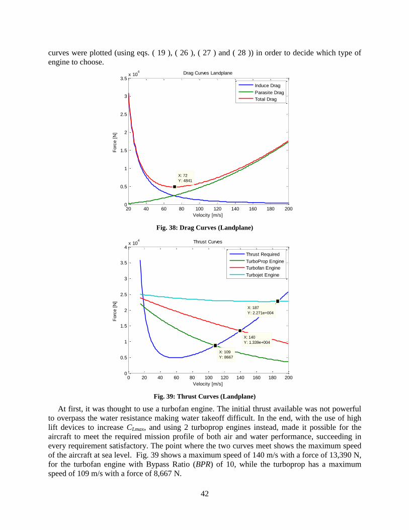
42
curves were plotted (using eqs. ( 19 ), ( 26 ), ( 27 ) and ( 28 )) in order to decide which type of
engine to choose.
Fig. 38: Drag Curves (Landplane)
Fig. 39: Thrust Curves (Landplane)
At first, it was thought to use a turbofan engine. The initial thrust available was not powerful
to overpass the water resistance making water takeoff difficult. In the end, with the use of high
lift devices to increase CLmax, and using 2 turboprop engines instead, made it possible for the
aircraft to meet the required mission profile of both air and water performance, succeeding in
every requirement satisfactory. The point where the two curves meet shows the maximum speed
of the aircraft at sea level. Fig. 39 shows a maximum speed of 140 m/s with a force of 13,390 N,
for the turbofan engine with Bypass Ratio (BPR) of 10, while the turboprop has a maximum
speed of 109 m/s with a force of 8,667 N.
20 40 60 80 100 120 140 160 180 2000
0.5
1
1.5
2
2.5
3
3.5x 10
4
X: 72
Y: 4841
Velocity [m/s]
Forc
e [
N]
Drag Curves Landplane
Induce Drag
Parasite Drag
Total Drag
0 20 40 60 80 100 120 140 160 180 2000
0.5
1
1.5
2
2.5
3
3.5
4x 10
4
X: 109
Y: 8667
Velocity [m/s]
Forc
e [
N]
Thrust Curves
X: 140
Y: 1.339e+004
X: 187
Y: 2.271e+004
Thrust Required
TurboProp Engine
Turbofan Engine
Turbojet Engine

43
Using eq. ( 20 ) and the CLmax provided, the Stall speed of the aircraft at sea level is 43.13 m/s.
The maximum coefficient of drag was calculated by assuming the landplane was cruising
90% of the maximum speed at a cruising altitude of 4,200 m. Table 8 shows the flat plate drag
breakdown of the landplane to obtain parasite drag. Calculations of induced drag as well as
compressibility drag (which is neglected) are also shown.
Table 8: Flat Plate Drag Area Breakdown (Landplane)
Flat Plate Drag Area [m2] Aircraft
Fuselage 0.152
Wing 0.323
Horizontal Tail 0.079
Vertical Tail 0.056
Engines 0.101
Upsweep 0.389
Total 1.154
Drag Cdp 0.033
Cdi 0.0095
Cdw 5.3e-008
Cd 0.043
4.1.4. Flight Performance
The air performance of the aircraft must be analyzed in order to observe if the landplane meets
the requirements stated in the mission profile. The flight performance of the aircraft was
calculated with the obtained maximum speed (109 m/s). A cruise speed 90% of the total
maximum speed was assumed to calculate the flight performance of the landplane aircraft in
order to obtain an efficient mission in which compromising the excess caused by the increase in
drag due to the maximum speed.
The climb speed (Vc) of the aircraft was calculated using eq. ( 21 ). It was found the aircraft
has a maximum Vc of 6.6 m/s at sea level and a Vc of 2.8 m/s at cruising altitude of 4,200 m.
Assuming a linear relation between Vc and altitude (H), a curve of Vc vs. H was plotted in order
to obtain the service and absolute ceilings of the aircraft shown in Fig. 40.
The absolute ceiling of the aircraft is shown to be 6,721 m at a Vc of 0.5 m/s. The service
ceiling is 7,273 m at Vc = 0 m/s. With the service ceiling, the maximum speed, and stall speed of
the aircraft, an altitude envelope was created, Fig. 41. An altitude envelope generally shows the
relation between speed at level flight and altitude although other variables are also possible. It
takes more effort to make than an extra power calculation, but in turn provides much more
information such as ideal flight altitude. The plot typically looks something like an upside-down
U and is commonly referred to as a doghouse plot due to its resemblance to a doghouse.
The outer edges of the diagram, the envelope, show the possible conditions that the aircraft
can reach in straight and level flight. For instance, this aircraft can fly at altitudes up to about
7,000m, at which point some external influence means it can no longer climb. The aircraft can
also fly at up to Mach 0.32 at sea level, but no faster. This outer surface of the curve represents
the zero-extra-power condition. All of the area under the curve represents conditions that the
plane can normally fly at, for instance, this aircraft can fly at Mach 0.45 at 7,000 m, and doing so

44
would require something less than full power. Flying outside the envelope is possible, since it
represents the straight-and-level condition only. For instance diving the aircraft allows higher
speeds, using gravity as a source of additional power.
Fig. 40: Landplane Climb Diagram
Fig. 41: Altitude Envelope of Landplane
Next, calculations of the range and endurance of the aircraft were performed. The aircraft
must be able to have a range of around 1,000 km. To calculate the range and endurance, every
segment of the mission (takeoff, climb, cruise, descent, and landing) was calculated.
Several assumptions are taken into consideration to calculate each flight segment. The
landplane is designed with high lift devices (flaps), then it is assumed an increase in CL at
takeoff, hence an increase in CD. The landplane takes off at 1.2*VS0 and a friction coefficient of
0.03 was considered for dry concrete. Last, an increase in drag due to the landing gear extended
0 1 2 3 4 5 6 70
1000
2000
3000
4000
5000
6000
7000
8000
X: 0.5
Y: 6721
Rate of Climb [m/s]
Altitude [
m]
Climb DiagramX: 0
Y: 7273
0.1 0.15 0.2 0.25 0.3 0.35 0.4 0.45 0.50
1000
2000
3000
4000
5000
6000
7000
8000
X: 0.4469
Y: 7273
Mach
Altitude [
m]
Altitude Envelope
X: 0.32
Y: 0
X: 0.189
Y: 7273
X: 0.1267
Y: 0

45
was also considered. For descent, a descent angle of 3o was used. Finally, for landing the same
assumptions for takeoff are taken into consideration. The same increase in CD due to landing
gear extended was considered. The increase in CL and CD due to high lift devices was used,
however higher values due to full configuration were assumed. The same friction coefficient for
dry concrete was used; however a new friction coefficient was introduced when the aircraft
applied the brakes. Finally, the aircraft was designed with spoilers in order to decrease CL, where
CD was also assumed to increase.
The elaboration of the mass fuel breakdown was elaborated based on the performance of the
aircraft and the thrust available produced. The two turboprop engines producing a total of 25,500
N of static sea level thrust were enough to meet the mission profile. Calculation of the mass fuel
weight was elaborated using eqs. ( 8 ) and ( 9 ). Since the amount of fuel needed for each flight
segment depends on the amount of time and fuel consumption, eqs. ( 24 ) and ( 25 ) were used to
calculate the amount of fuel consumption and selecting the appropriate throttle settling for each
flight segment. Last, using the empirical equation of thrust available for a turboprop engine was
elaborated using eq. ( 26 ).
With the assumptions considered, the amount of distance, time and fuel were calculated for
each segment and are shown in Table 9. The cruise endurance and range of the aircraft were
calculated using eqs. ( 22 ) and ( 23 ). The complete equations for calculating the mission
segments are shown in Appendix A.3.
Table 9: Endurance and Range (Landplane)
Endurance [hr] Range [km] Fuel [kg]
Takeoff 0.005 0.5 14
Climb 0.18 62.4 57
Cruising 2.81 992.3 1100
Descent 0.28 80 41
Landing 0.007 0.8 3
Total 3.28 1136 1215
The total fuel weight of the mission was 1,215 kg. Considering 75 kg for reserves and 10 kg
for taxi manoeuvres, the total required mass of fuel is 1,300 kg. The estimated initial Gross
Weight (GWest) enter into the LOTS code was 6,600 kg, then the total payload for maximum fuel
and using eq. ( 7 ) was 1,400 kg. The total payload the aircraft accounts for crew weight,
avionics, cargo or passengers, etc. To account the aircraft is able to carry more payload than
what was calculated (1,400 kg), it is assumed the aircraft has a capability to carry a maximum of
1,700 kg, for that instance reducing fuel weight to 1,000 kg.
A tradeoff between payload and range of the aircraft can be illustrated in a payload-range
diagram. There are 3 factors to consider in a payload-range diagram. The top horizontal line
shows the maximum payload that the aircraft is structurally permitted to carry. The vertical line
represents the total range of the aircraft. Finally, the diagonal line after the range at maximum
payload point shows how reducing the payload allows increasing the fuel (and range) when
taking off with the maximum take-off weight. This diagonal line represents the tradeoff between
maximum fuel and maximum payload. Smaller the diagonal line, smaller the tradeoff, therefore
obtaining more productivity weight between payload and fuel. The payload-range diagram for
this aircraft is shown in Fig. 42.
Finally, Fig. 43 shows the manoeuvring envelope of the landplane. The maximum positive
load factor is 4.4 and the maximum negative load factor for dives is -1.76. These values are

46
obtained from FAR 23/25 for a utility aircraft. Fig. 43 also shows the gust envelope. The gust
speeds are obtained from Raymer [27] and the maximum gust speed is a function of altitude
only. As can be seen from the figure, the gust loads do not exceed the manoeuvring loads.
Since the LOTS code complies with all the mission requirements, final aircraft parameters
and performance are given ending the iteration.
Fig. 42: Payload Range Diagram (Landplane)
Fig. 43: Maneuvering and Gust Envelopes (Landplane)
0 200 400 600 800 1000 12000
200
400
600
800
1000
1200
1400
1600
1800
X: 865.2
Y: 1700
Range [km]
Paylo
ad [
kg]
Payload Range Diagram
X: 1136
Y: 1400
X: 1193
Y: 0
40 50 60 70 80 90 100 110-2
-1
0
1
2
3
4V-n Diagram
Velocity [m/s]
Load F
acto
r

47
4.2. Floating Device Results After elaborating the landplane aircraft, the next step in the design is the elaboration of the
floating device. The advance optimization code calls the FOTS code to iterate and optimize the
most efficient floating device the seaplane should use. As explained, the FOTS code can
elaborate a boat hull with wing tip floats, mid wing stabilizers, or side floats creating a trimaran
configuration. The proposed solution is the integration of a trimaran design to the floating
device. Therefore, in order to prove the advantage of the trimaran over other configurations, the
results of the 3 design configurations are compared and analyzed.
4.2.1. Weight Breakdown
First, based on the FOTS code, the first step of the sizing iteration is the calculation of the
weight components of the floating device. Based on eqs. ( 42 ) - ( 44 ), the following weights for
the floating devices are found.
It is seen in Table 10, the weight increase of the seaplane with a trimaran configuration, mid
wing stabilizers and wing tip stabilizers. For the trimaran, using maximum fuel, the payload
decreased 400 kg. Comparing with wing tip floats, the payload weight reduced 300 kg, in which
the difference is not excessive. In the end, the trimaran configuration shows larger empty weight
compared to the other configurations. The reason is in the size of the stabilizers, in this case the
outriggers. This increase in size depends on the hydrostatic and hydrodynamic performance of
the seaplane, which is explained further in detail. The lost payload capacity of the trimaran can
be recovered by the outriggers in which extra storage for fuel or luggage could be used.
Table 10: Weight Component Breakdown
Weights [kg] Landplane Seaplane Trimaran Seaplane Mid Wing Seaplane Wing Tip
Boat Hull 0 220 220 220
Outriggers 0 130 0 0
Mid Stabilizers 0 0 70 0
Wing Tip Floats 0 0 0 50
Strutting 0 50 60 30
Empty Weight 3,900 4,300 4,250 4,200
Max Fuel 1,300 1,300 1,300 1,300
Payload 1,400 1,000 1,050 1,100
Gross Weight 6,600 6,600 6,600 6,600
4.2.2. Geometry calculations
The next calculation done by the FOTS code is sizing the geometry of the floating device.
Using the equations from the subsection of the geometry calculations from the theory section,
sizing of the main hull, outrigger, mid wing stabilizer and wing tip stabilizer was elaborated.
Table 11 shows the dimensions of each of the floating devices.
When the FOTS code is sizing the main boat hull of the aircraft, it checks if the length of the
hull does not exceeds the length of the fuselage, in this case 14.47 [m]. Finding a suitable
Slenderness Ratio (SLR) is vital to attain the desire design. In first instance, the first guessed SLR
used was of 12 to obtain a performance cruiser seaplane. Then, a suitable Spray Coefficient (k)
equal 0.0825 to have heavy but acceptable spray was used. The FOTS code decided the most
optimum SLR for the main hull was 7 with a k of 0.0975. One of the big issues the FOTS code

48
encountered to attain the desired sizing was to not exceed the fuselage length. If using a SLR=12,
k=0.0825 and not exceeding the 14.47 [m] of fuselage length, the beam of the hull became
excessively large, showing a bad aspect to the seaplane. In the end, the beam of the hull was 2.03
[m], which does not exceed the diameter of the fuselage, making an aesthetic design. To
counteract the excess in spray, chines are placed at the edges of the hull to reduce this
complication. In the end, the SLR and k used for the outriggers (14 and 0.08, respectively) are
satisfactory to attain the desired design.
Some of the dimensions are calculated using the equations stated; however, the angles
(afterbody, and keel) were selected based on the literature review [36], the aspect of the
stabilizers, and other aspects that increased the optimization of the design. The forebody deadrise
angle is obtained using eq. ( 53 ), from the FAR requirements. Then based on FAR requirements
[66], the following curve was plotted to identify the desired forebody deadrise angle that meets
the landing requirements shown in Fig. 44. To obtain a slender trimaran, the forebody deadrise
angle of the main hull used was 30o, with a load factor of 1.716. For the outrigger, an angle of
45o was used, with a load factor of 1.19.
As explained before, the weight of the outriggers is larger compared to the stabilizers or wing
tip float. The size of the stabilizers depends on the righting moment from eq. ( 39 ), and the
clearance distance; With greater clearance distance, smaller stabilizers.
With the dimensions of the main hull, the outriggers, the stabilizers and the wing tip floats
calculated, the new floating device was added to the landplane aircraft to create the seaplane.
Fig. 45, Fig. 46 and Fig. 47 show the 3 different configurations of the seaplane.
Table 11: Floating Device Dimensions
Main Hull Outrigger Stabilizer Wing Tip
Slenderness Ratio 7 14 - -
Spray Coefficient 0.0975 0.08 - -
Beam [m] 2.03 0.51 0.95 0.65
Length [m] 14.47 7.13 3.82 2.60
Forebody [m] 6.99 3.38 1.81 1.23
Afterbody [m] 7.48 3.75 2.01 1.37
Bow Height [m] 1.32 0.53 0.48 0.32
Step Height [m] 0.18 0.05 0.09 0.06
Forebody Angle 30o 45
o 15
o 15
o
Afterbody Angle 22o 40
o 20
o 15
o
Keel Angle 7o 7
o 7
o 7
o
Volume [m3] 17.43 1.51 1.74 0.55
Clearance [m] - 1.74 3.00 9.54
Stagger [m] - -0.90 2.25 2.25

49
Fig. 44: Water Landing Load Factor Curve
Fig. 45: CAD Model of Seaplane with Wing Tip Floats
Fig. 46: CAD Model of Seaplane with Nacelle Support Stabilizers
0 5 10 15 20 25 30 35 40 45 500
2
4
6
8
10
12
14
16
18
X: 30
Y: 1.716
Forebody Deadrise Angle [deg]
Load F
acto
r
Load Factor Curve
X: 45
Y: 1.19

50
Fig. 47: CAD Model of Seaplane with Trimaran Concept
4.2.3. Hydrostatic Stability
The next goal of the FOTS sizing code is to meet the hydrostatic stability. Using the approach
from eqs. ( 46 ) - ( 48 ) in the theory section, the following hydrostatic results were obtained. The
center of gravity, center of buoyancy, metacentre and metacentric height are shown in Table 12.
Using the approach from eq. ( 47 ), the metacentric height was calculated; The center of gravity
was found using SOLIDWORKS mass properties analysis; the center of buoyancy was
calculated by dividing the volume displacement over the water line area.
To show an example of the location of the metacentre (GM), center of buoyancy (CB), and the
centre of gravity (CG), a model of a seaplane was elaborated shown in Fig. 48.
Using eq. ( 48 ), the data obtained from Table 12 and the required displacement of each
component, the following plot was graphed showing the Righting Moment (RM) as a function of
heel angle θ, in Fig. 49.
Table 12: Hydrostatic Stability (Seaplane)
Distance from Keel [m] Trimaran Stabilizer Wing Tip Float
Draft Line 0.48 0.48 0.53
Center of Bouyancy 0.45 0.45 0.51
Center of Gravity 1.75 1.84 1.84
Metacentre 1.61 4.13 17.93
Metacentric Height 0.32 2.75 16.60
Fig. 48: CAD Model of Seaplane transverse Metacentre, Centre of Gravity, and Buoyancy
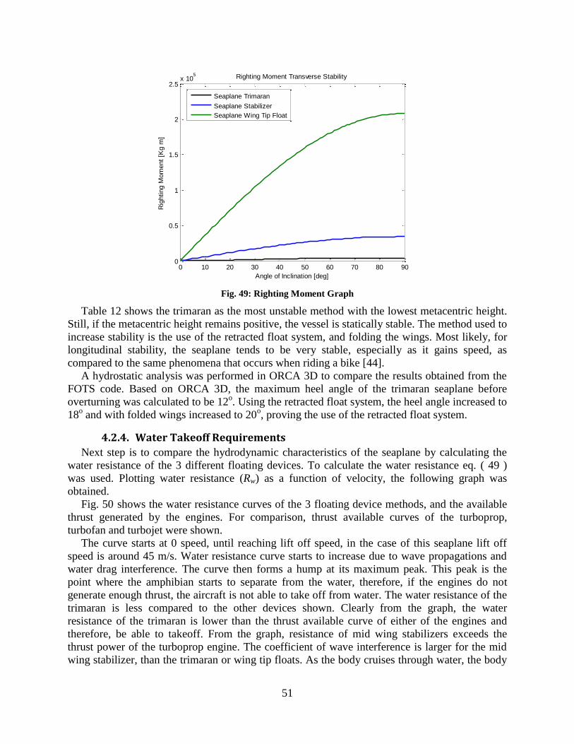
51
Fig. 49: Righting Moment Graph
Table 12 shows the trimaran as the most unstable method with the lowest metacentric height.
Still, if the metacentric height remains positive, the vessel is statically stable. The method used to
increase stability is the use of the retracted float system, and folding the wings. Most likely, for
longitudinal stability, the seaplane tends to be very stable, especially as it gains speed, as
compared to the same phenomena that occurs when riding a bike [44].
A hydrostatic analysis was performed in ORCA 3D to compare the results obtained from the
FOTS code. Based on ORCA 3D, the maximum heel angle of the trimaran seaplane before
overturning was calculated to be 12o. Using the retracted float system, the heel angle increased to
18o and with folded wings increased to 20
o, proving the use of the retracted float system.
4.2.4. Water Takeoff Requirements
Next step is to compare the hydrodynamic characteristics of the seaplane by calculating the
water resistance of the 3 different floating devices. To calculate the water resistance eq. ( 49 )
was used. Plotting water resistance (Rw) as a function of velocity, the following graph was
obtained.
Fig. 50 shows the water resistance curves of the 3 floating device methods, and the available
thrust generated by the engines. For comparison, thrust available curves of the turboprop,
turbofan and turbojet were shown.
The curve starts at 0 speed, until reaching lift off speed, in the case of this seaplane lift off
speed is around 45 m/s. Water resistance curve starts to increase due to wave propagations and
water drag interference. The curve then forms a hump at its maximum peak. This peak is the
point where the amphibian starts to separate from the water, therefore, if the engines do not
generate enough thrust, the aircraft is not able to take off from water. The water resistance of the
trimaran is less compared to the other devices shown. Clearly from the graph, the water
resistance of the trimaran is lower than the thrust available curve of either of the engines and
therefore, be able to takeoff. From the graph, resistance of mid wing stabilizers exceeds the
thrust power of the turboprop engine. The coefficient of wave interference is larger for the mid
wing stabilizer, than the trimaran or wing tip floats. As the body cruises through water, the body
0 10 20 30 40 50 60 70 80 900
0.5
1
1.5
2
2.5x 10
5
Angle of Inclination [deg]
Rig
hting M
om
ent
[Kg m
]
Righting Moment Transverse Stability
Seaplane Trimaran
Seaplane Stabilizer
Seaplane Wing Tip Float

52
creates waves along its path as shown in Fig. 35. Since seaplanes use lateral stabilizers and a
main hull, the stabilizers as well as the hull create wave patterns along its way. The point where
this two propagated waves collide generates a phenomena that increases the viscous drag of the
seaplane. To reduce this point, the stabilizers must have a low clearance distance or very high as
in the case of the trimaran and wing tip floats.
As explained before, at first instance, using turboprop engines with a sea level thrust of
25,500 N, did not generated enough thrust to overcome the water resistance. It was then assumed
the aircraft uses high lift devices that increase the CLmax from 1.63 to 2.08.
Fig. 50: Water Resistance Curves and Thrust Available
4.2.5. Aerodynamic Drag
Now it is essential to think on techniques to reduce the aerodynamic drag caused by the
outriggers, stabilizers, or wing tip floats in order to increase the flight performance of the
seaplane. A useful technique is to retract the floats into a position where the floats create a single
body shape, either to the wing or the fuselage. The following images show how the floats were
being retracted.
Fig. 51: Wing Tip Floats Retracted into the Wing Tip
0 5 10 15 20 25 30 35 40 450
0.5
1
1.5
2
2.5
3x 10
4
Velocity [m/s]
Resis
tance [
N]
Resistance Curves
Water Resistance Trimaran
Water Resistance Stabilizer
Water Resistance Wing Tip Float
Thrust Available Prop
Thrust Available JET
Thrust Available TurboFAN

53
Fig. 52: Nacelle Wing Stabilizers Retracted
The strutting on the wing tip floats and stabilizers compromises some the wing structural
support, and requires a complex retracting system with strong and heavy material required. This
also compromises an excess in weight, reducing the useful weight the aircraft is able to carry. In
the case of the trimaran, the strutting is placed through the boat hull, in which the boat hull and
the entire fuselage are built as a single component of the aircraft, reducing the need for strong
material used for the strutting. The outriggers are retracted into the boat hull, creating a
“smoother” body that results for less aerodynamic drag, as shown in Fig. 53 [59].
Fig. 53: Trimaran Outriggers Retracted unto the Boat Hull
The same approach to calculate the coefficient of drag for the landplane was applied to the
floating device. It is explained when an odd shape component is being calculated, an increase in
drag form interference factor must be added to the actual value [60]. It is also explained: “The
form factor is a measure of how “streamlined” the component is; it is a function of the
component thickness-to-length ratio” [68]. In this case, the form interference factor (F) of a
flying boat hull must increase by a 50%, and for floats from 75%-300%, depending on the shape.
In the end, the boat hull is designed as a smooth, slender body. Then, it was assumed that the
interference factor for the boat hull had an increase of 10%, rather than 50% increased, due to the
perfect aerodynamic shape mounted of the hull with respect to the fuselage. A comparison of the
decrease in parasite drag for the floating devices in retracted position, and extended position is

54
elaborated theoretically in Table 13. Calculation of the parasite drag was done with a flat plate
drag area breakdown of each of the 3 configurations for comparison.
As expected, the greatest increase in drag are the mid wing stabilizers. Wing Tip floats show
the least increased in drag due to its small size compared to the other stabilizers, and the
retractable system assembles the tip floats as wing tip tanks.
Table 13: Flat Plate Drag Area Breakdown Floating Devices
Flat Plate Trimaran Mid Wing Stabilizers Wing Tip Floats
Drag Area [m2] Extended Retracted Extended Retracted Extended Retracted
Boat Hull 0.127 0.105 0.127 0.105 0.127 0.105
Stabilizer 0.075 0.051 0.09 0.072 0.044 0.034
Strutting 0.005 0.002 0.009 0.003 0.004 0.001
Total 0.185 0.158 0.204 0.18 0.153 0.14
Cdp 0.0059 0.0045 0.0065 0.0052 0.0050 0.0040
A comparison of the increase in parasite drag, with the landplane aircraft is made to show the
increment in percent and the advantage of using the retractable system. Table 14 shows the
values of the increase in parasite drag of the trimaran seaplane.
Another solution in solving the increase of drag is by retracting the floats inside the boat hull
as explained earlier and shown in Fig. 26. There is nearly a 3% decreased in parasite drag
compared to the floats in the retracted position.
Table 14: Flat Plate Drag Area Breakdown Trimaran Seaplane
Landplane Seaplane
[Extended]
Seaplane
[Retracted]
Seaplane
[No Floats]
Drag Area [m2] 1.154 1.361 1.312 1.269
Cdp 0.033 0.039 0.038 0.036
Cdp Increment - 0.006 0.005 0.003
Drag Increase - 12.24% 9.63% 6.63%
4.2.6. Flight Performance
With the increase in drag, new calculations of the flight performance for the seaplane were
performed. Comparison of the landplane performance and the trimaran seaplane is made. The
required thrust increases if the coefficient of drag increases (CDp), hence compromising the flight
performance of the seaplane. Therefore, the maximum speed of the seaplane must decrease as
shown in Fig. 54.
The maximum speed of the seaplane with floats extended at sea level decreased to 103 m/s.
The thrust required increased due to the increase in coefficient of drag, therefore the rate of
climb of the seaplane decreased. The seaplane with extended floats has a lower rate of climb, as
compared to seaplane with retracted floats. The seaplane takes longer and more distance to climb
the desire altitude, i.e. the absolute and service ceilings decrease as shown from Fig. 55.
The calculations of each of the flight segments for the trimaran seaplane take into
consideration the same assumptions described for the landplane. The only difference is takeoff
and landing in which the seaplane does not apply brakes; instead water resistance comes into
action. For water takeoff, high lift devices increase the CLmax. Also, the increase in Cd due to the
floating device is then added. At takeoff and landing, the Cd increase with the outriggers

55
extended is first used. At climb, cruise and descent, the outriggers are retracted, decreasing Cd.
Table 15 shows a comparison of the endurance and range of the landplane, the seaplane with
outriggers in retracted position, and seaplane with outriggers in extended position. As shown,
there is an increase of around 100 km of the trimaran seaplane with the outriggers retracted,
compared to the outriggers in the extended position.
Fig. 54: Thrust Curves (Landplane and Trimaran Seaplane)
Fig. 55: Altitude Envelope (Landplane and Trimaran Seaplane [Retracted])
Table 15: Endurance and Range of each Flight Segment
Landplane Seaplane [Rect] Seaplane [Ext]
Endurance [hr] 3.28 3.11 2.88
Range [km] 1,136 1,017 933
0 50 100 1500
0.5
1
1.5
2
2.5
3
3.5
4x 10
4
Velocity [m/s]
Forc
e [
N]
Thrust Curves
X: 103
Y: 9198X: 109
Y: 8667
Thrust Required Landplane
Thrust Required Seaplane
TurboProp Engine
0.1 0.15 0.2 0.25 0.3 0.35 0.4 0.45 0.50
1000
2000
3000
4000
5000
6000
7000
8000
X: 0.4249
Y: 7089
Mach
Altitude [
m]
Altitude Envelope
X: 0.1873
Y: 7089
Landplane
Seaplane
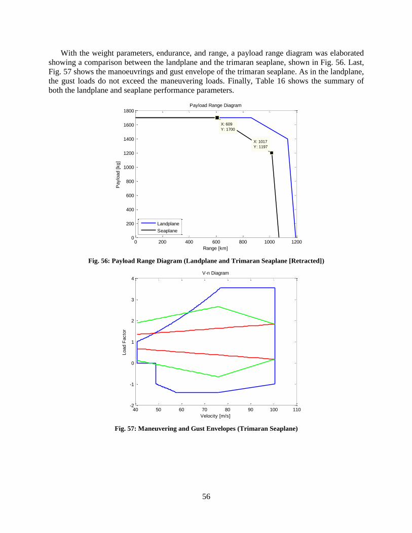
56
With the weight parameters, endurance, and range, a payload range diagram was elaborated
showing a comparison between the landplane and the trimaran seaplane, shown in Fig. 56. Last,
Fig. 57 shows the manoeuvrings and gust envelope of the trimaran seaplane. As in the landplane,
the gust loads do not exceed the maneuvering loads. Finally, Table 16 shows the summary of
both the landplane and seaplane performance parameters.
Fig. 56: Payload Range Diagram (Landplane and Trimaran Seaplane [Retracted])
Fig. 57: Maneuvering and Gust Envelopes (Trimaran Seaplane)
0 200 400 600 800 1000 12000
200
400
600
800
1000
1200
1400
1600
1800
X: 609
Y: 1700
Range [km]
Paylo
ad [
kg]
Payload Range Diagram
X: 1017
Y: 1197
Landplane
Seaplane
40 50 60 70 80 90 100 110-2
-1
0
1
2
3
4V-n Diagram
Velocity [m/s]
Load F
acto
r

57
Table 16: Summary of major design values (Landplane and Trimaran Seaplane)
Parameters Landplane Seaplane
Gross Weight [kg] 6,600 6,600
Empty Weight [kg] 3,900 4,300
Max Speed [km/hr] 392 370
Rate of Climb [m/s] 6.6 6.2
Absolute Ceiling [m] 7,273 7,089
Endurance [hr] 3.28 3.11
Maximum Range [km] 1,136 1,017
4.3. Design Analysis
4.3.1. SOLIDWORKS Computer Aided Design (CAD) Analysis
With the preliminary design of the amphibious aircraft finalized, a 3-D model was constructed
using SOLIDWORKS. This model was used to analyze the center of gravity and center of
buoyancy as well as to run Orca3D test cases. To obtain valid comparisons between the various
analysis programs that were used to validate and improve the optimization code, it was very
important to keep the 3-D model as true as possible to the final optimized design that was output
by the sizing code.
While the output file specifies the exact geometry of boat hull, floats, and wing, it only
provides general dimensions for the fuselage and engine, although the code does have relative
positions for all the components. This means that these last two components must undergo
detailed design not specified by the optimization code.
The sizing code output specifies the length, width and height of the boat hull fuselage of the
aircraft, but does not specify any further details, such as the shape of the bottom of the forebody
and afterbody. Both of these design factors affects the performance of the amphibious aircraft
while it is on the water, especially in respect to its takeoff performance.
Some of the important aspects SOLIDWORKS performs are to identify the center of gravity
of the model in the mass properties tool. This application calculates properties such as mass,
density, and volume, based on the model geometry and material properties. This useful
application was necessary to identify the center of gravity of the seaplane, and to compare the
moments of inertia. With the center of gravity identified, it was useful to calculate the center of
buoyancy of the model. The identified center of gravity and calculated center of buoyancy was
compared to the identified centers elaborated by ORCA 3D.
An important concern that arises by placing a hull under a fuselage may be related to the
structural force the fuselage must support. SOLIDWORKS performs basic structural analysis to
analyze the stress and displacement of the model.
4.3.1.1. Results SOLIDWORKS SimulationXpress offers an easy stress analysis tool for design analysis
users. It performs a basic analysis of the effects of a force applied to a certain body of a model.
For this case, a simple structural analysis of the boat hull was performed to analyze the impact
the hull withstands at water landing.
SimulationXpress starts by identifying the body to analyze. In this case, the main hull is
analyzed for water landing impact. Then, a fixture must be added. Applying a fixture keeps the

58
part from moving when loads are applied, though a face with fixtures are treated as perfectly
rigid body, in which can cause unrealistic results. For this analysis, the fuselage is treated as the
fixture, as shown in Fig. 58.
Fig. 58: Trimaran Seaplane Fuselage Fixture
Next, applying the force to the body (in this case the boat hull) must be selected. The total
force applied was around 60,000 N, which is based on the Gross Weight at landing (6,200 kg).
The force is applied at forebody of the hull since this is the main part of the hull that receives
most of the landing impact, shown in Fig. 59.
Fig. 59: Trimaran Seaplane Load Force at Afterbody Hull
The next step is to choose the material of the hull. It was decided to use composite materials,
in this case Glass Laminate Aluminium Reinforced Epoxy (GLARE). This material is light,
strong and has an advantage against corrosion. After selecting the fixture, the load and material,
the simulation starts by meshing the model. SOLIDWORKS performs the meshing by the
elaboration of Finite Element Analysis (FEA), which connects small pieces of the model called
elements which then share common points called nodes. The example mesh figure of the
trimaran seaplane is shown in Fig. 60.
Finally, the simulation performs a Von Mises Stress and a displacement analysis. The
resultant action shows an image with the hull deformed. The image is a mere exaggeration just to
visualize where the deformation is taken place. Most of the deformed body takes place around

59
the step of the hull. Since the seaplane must land in an angle, the deformation is found to be
consistent to an actual realistic result. The maximum deformation encountered by the hull is of
4.5e-4 mm. Maximum Von Mises Stress is 0.052 N/mm2 at the point shown in Fig. 61.
Fig. 60: Trimaran Seaplane Mesh
Fig. 61: Trimaran Seaplane Von Mises Stress Analysis
4.3.2. ORCA 3D
Orca3D is a suite of tools used for naval architectural design and analysis that were written as
a plug-in for the Rhinoceros 3-D modeling software. For this research, Orca3D was used to
determine if the amphibious aircraft that was output by the sizing code had satisfactory
longitudinal and transverse stability in the water. The stability of the aircraft in water is
determined by finding the location of the longitudinal and transverse metacenters.
Classically, Simpson’s Rule was the primary tool used in designing boat hulls. Simpson’s
Rule is a method of numerical integration and is governed by
∫ ( )
( ( ) (
) ( ))
( 54 )

60
Using this approximation, a designer could calculate the location of the longitudinal and
transverse metacenters, as well as the center of buoyancy and center of floatation, of a boat hull
being designed.
Computer aided hull design has been becoming more and more prominent in recent years, as
it offers advantages over traditional design methods. A majority of CAD representations of a
boat hull are curve-surfaces. Orca3D generates a mesh from this surface to calculate most of its
hydrostatic and stability parameters. With a mesh created, Orca3D then uses Simpson’s Rule to
numerically integrate between the mesh nodes. This method of computer aided mesh generation
and numerical analysis leads to more accurate results, as it doesn’t rely on a manually calculated
station model, which has a tendency to miss local hull features, such as discontinuities and
curvature changes.
According to Sederberg [69], the de-facto CAD standard for representing curved surfaces
since the 1970’s has been the non-uniform rational B-splines (NURBS). NURBS are the only
free-form surface type supported in the IGES file format, which is the most popular format for
transferring data between CAD software. Unfortunately, NURBS have two weaknesses that
impact hull design and analysis. First, to make hull optimization and analysis easier, it is helpful
to have the entire hull represented with a single surface. Unfortunately, due to NURBS needing
rectangular topography when making its mesh, a complicated hull cannot always be represented
by a single surface. Secondly, control node points for a NURBS surface must lie in a rectangular
grid, which leads to there being a large number of control points that carry no significant
geometric information and only serve to increase calculation time. Fig. 62 illustrates the
drawbacks of the NURBS model. The personal watercraft depicted is divided into 13 surfaces in
order to maintain the required rectangular topography. Also, many of the nodal points are
unnecessary and are merely included to satisfy rectangular shape constraints.
To address the limitations of using NURBS to model complex boat hulls, T-Splines were
introduced. T-Splines are not limited to a rectangular geometry, which significantly reduces the
number of superfluous points needed to complete the mesh as well as make the modeling of a
complex body with a single surface possible. In the NURBS mesh, all the interior control points
have a valence of four, which means that all the interior control points touch four edges. A T-
Spline mesh (T-Mesh) allows control points to have valence other than four. These points are
shown in Fig. 62 as yellow dots. The ability to have nodal points with different valence values
gives T-Splines the ability to model any surface using a single T-Mesh. T-Splines were
integrated into Orca3D to decrease calculation time as well as increase the accuracy of the
calculations by removing discontinuities between surface meshes.
Fig. 62: Personal Watercraft Modeled as a NURBS and a T-Spline [69]
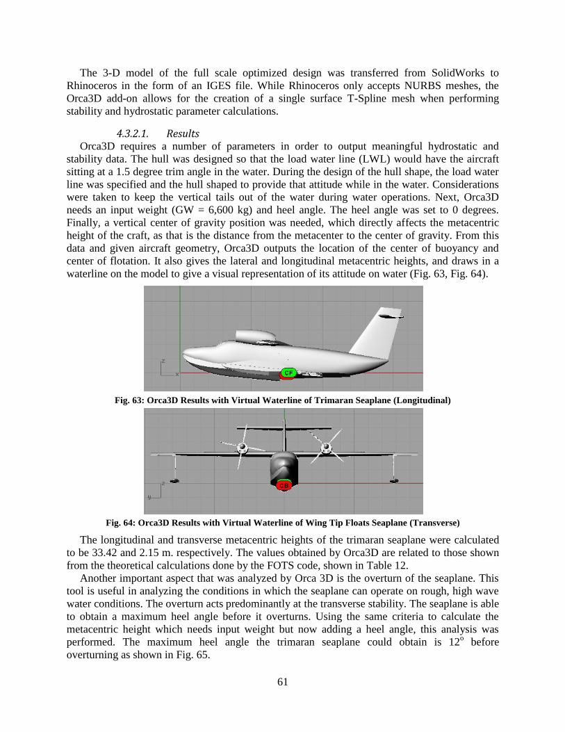
61
The 3-D model of the full scale optimized design was transferred from SolidWorks to
Rhinoceros in the form of an IGES file. While Rhinoceros only accepts NURBS meshes, the
Orca3D add-on allows for the creation of a single surface T-Spline mesh when performing
stability and hydrostatic parameter calculations.
4.3.2.1. Results Orca3D requires a number of parameters in order to output meaningful hydrostatic and
stability data. The hull was designed so that the load water line (LWL) would have the aircraft
sitting at a 1.5 degree trim angle in the water. During the design of the hull shape, the load water
line was specified and the hull shaped to provide that attitude while in the water. Considerations
were taken to keep the vertical tails out of the water during water operations. Next, Orca3D
needs an input weight (GW = 6,600 kg) and heel angle. The heel angle was set to 0 degrees.
Finally, a vertical center of gravity position was needed, which directly affects the metacentric
height of the craft, as that is the distance from the metacenter to the center of gravity. From this
data and given aircraft geometry, Orca3D outputs the location of the center of buoyancy and
center of flotation. It also gives the lateral and longitudinal metacentric heights, and draws in a
waterline on the model to give a visual representation of its attitude on water (Fig. 63, Fig. 64).
Fig. 63: Orca3D Results with Virtual Waterline of Trimaran Seaplane (Longitudinal)
Fig. 64: Orca3D Results with Virtual Waterline of Wing Tip Floats Seaplane (Transverse)
The longitudinal and transverse metacentric heights of the trimaran seaplane were calculated
to be 33.42 and 2.15 m. respectively. The values obtained by Orca3D are related to those shown
from the theoretical calculations done by the FOTS code, shown in Table 12.
Another important aspect that was analyzed by Orca 3D is the overturn of the seaplane. This
tool is useful in analyzing the conditions in which the seaplane can operate on rough, high wave
water conditions. The overturn acts predominantly at the transverse stability. The seaplane is able
to obtain a maximum heel angle before it overturns. Using the same criteria to calculate the
metacentric height which needs input weight but now adding a heel angle, this analysis was
performed. The maximum heel angle the trimaran seaplane could obtain is 12o before
overturning as shown in Fig. 65.

62
Fig. 65 shows the trimaran seaplane when overturning. The outriggers turn in line with the
seaplane, where the right outrigger is sunk inside the water and the left outrigger is out in the air.
However, with the retractable float system, the outriggers are automated to stay in the water line,
giving the seaplane more stability. Applying this system into the Orca 3D analysis, the maximum
heel angle the seaplane trimaran can obtain increased to 18o.
Fig. 65: Trimaran Seaplane at 12
o Heel Angle before Overturning
Furthermore, the idea to obtain a seaplane that has outstanding water capability added the
solution to fold the wings to increase the heel angle of the seaplane. Folding the wings gives the
seaplane a better clearance when it is maneuvering in the water, especially in bodies of water
with too congested boats or ships. Using the retractable float system and folded wings, the heel
angle increased to 20o, shown in Fig. 66.
Fig. 66: Trimaran Seaplane at 20
o Heel Angle before Overturning
4.3.3. Software Validation
Based on researched [70], CAD programs have a high validity and reliability, hence high
accuracy for modeling. There are two common methods of 3-D models: Meshes and NURBS.
NURBS method is more accurate than meshes since a mesh represents flat triangles, while
NURBS are free form surfaces as explained before. SOLIDWORKS and Rhino uses NURBS
when modeling, making the C.G. calculation very accurate. That means the x-,y-, or z-
coordinate of any point can have a value ranging from as large as ±10308
to as small as ±10-308
.
Calculations can be accurate to 15 digits of precision in a range of ±1020
to ±10-20
. In the end,
there are a numerous industries that rely on CAD software such as SOLIDWORKS to perform
design modeling. Such examples are the American Institute of Aeronautics and Astronautics at
Arizona State University, BAE Systems, EAD Aerospace, Terrafugia, Inc., U.S. Army Research
Laboratory among many others [71].
63
5. 2050 Visionary Concept: Future Seaplane Transport
5.1. Introduction During the years of 1950 – 1980, the world was experiencing an exponential growth in
technological advances due to the superpower rivalry between the United States and the Soviet
Union. The aeronautical industry as well got caught in this expansion of technological
exploration. The empirical guidelines during those days were: higher, further, and faster. In the
late 1990’s, this exponential growth reached it maximum peak. The world was experiencing
economical problems, and certainly the aeronautical industry felt its effects. This “out of the
box” thinking that emerged during the postwar era is restricted now to the same problems,
money and social acceptance. Now, according to the European Vision 2020 guidelines, these
have become: more affordable, safer, cleaner and quieter [19]. The old empirical guidelines are
now forgotten, restricting the researcher’s mind to explore radical aeronautical designs.
In order to expand the designer’s mind, a modern vision with more radical, environmentally
efficient, and innovative technologies was created. The new vision is called Future Air Transport
Concept Technologies for 2050 in which the new guidelines will be: safer, quieter, cleaner and
efficient. An efficient concept adapts the early guidelines (higher, further, and faster), with no
restrictions in material, capital or infrastructure for planning, designing, testing, and constructing.
The research addressed aspects such as new ideas in airborne vehicles, including design, new
airport concepts as well as Air Traffic Management (ATM), alternative methods of air transport
system operation and their integration with other transport modes. Let us recall this is just a
radical way of thinking in order to expand the researcher’s mind with no restrictions what so
ever.
The purpose of this chapter was to create an example of this 2050 visionary aircraft concept,
in this case an advance amphibian aircraft. This amphibian aircraft was created on the basis of
the proposed past research, however improving the design into creating a futuristic idea. The new
proposed amphibian adapts advances capabilities such as Unmanned Aerial Vehicle (UAV)
mode, High Altitude and Long Endurance (HALE) capability, water and rescue missions, and
water bomber operations. The advance amphibian aircraft was created from a Blended Wing
Body (BWB) aircraft and converted into an amphibian by adapting the trimaran design concept
and the retracting float system creating an Advance Amphibian Blended Wing Body Aircraft
(AABWBA).
5.2. Review of Literature The BWB is a type of tailless flying wing design in which the wing and fuselage are blended
together into one seamless body in order to achieve significant improvements in performance
over the conventional aircraft, example shown in Fig. 67. Unlike the flying wing design, in
which the entire body of the aircraft is a wing, the BWB has a fuselage that is designed as a
wing. Therefore, the BWB has a fuselage section that is thicker than the flying wing which
allows it to accommodate more payloads. And, unlike a conventional aircraft, the BWB's
fuselage acts as a lifting body allowing it to generate lift, rather than acting as an interference
component [72].
In 1988, the McDonnell Douglas Company (now Boeing), along with NASA, conducted a
large study on the feasibility of a BWB passenger transport aircraft as an alternative to the
conventional cylindrical tube and wing transport. An initial study performed by Callaghan and
Liebeck in 1990 [73] showed that an 800 passenger BWB, when compared to a conventional
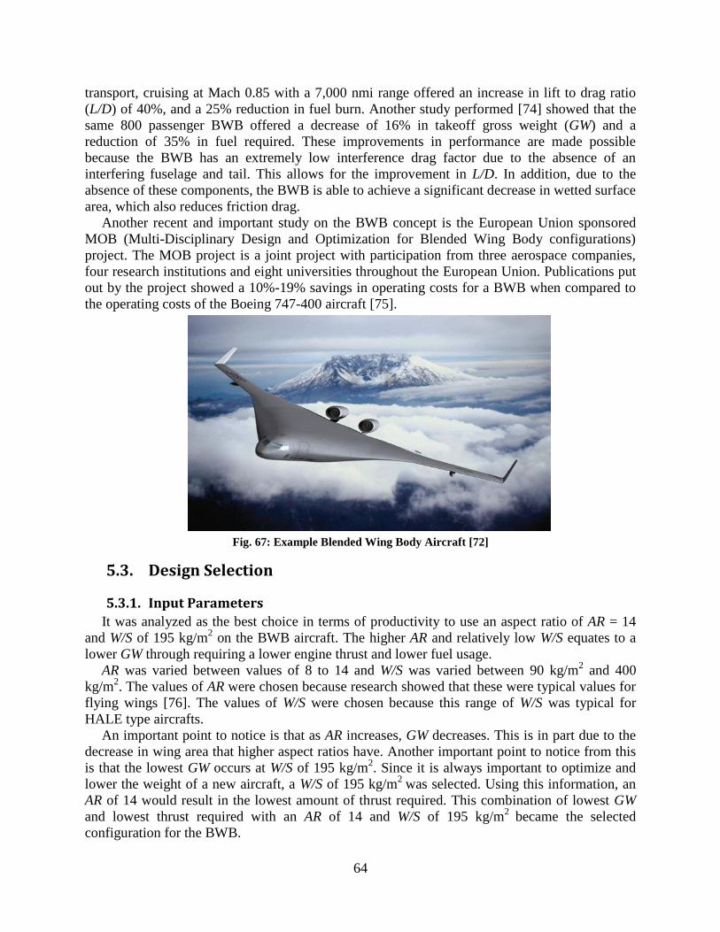
64
transport, cruising at Mach 0.85 with a 7,000 nmi range offered an increase in lift to drag ratio
(L/D) of 40%, and a 25% reduction in fuel burn. Another study performed [74] showed that the
same 800 passenger BWB offered a decrease of 16% in takeoff gross weight (GW) and a
reduction of 35% in fuel required. These improvements in performance are made possible
because the BWB has an extremely low interference drag factor due to the absence of an
interfering fuselage and tail. This allows for the improvement in L/D. In addition, due to the
absence of these components, the BWB is able to achieve a significant decrease in wetted surface
area, which also reduces friction drag.
Another recent and important study on the BWB concept is the European Union sponsored
MOB (Multi-Disciplinary Design and Optimization for Blended Wing Body configurations)
project. The MOB project is a joint project with participation from three aerospace companies,
four research institutions and eight universities throughout the European Union. Publications put
out by the project showed a 10%-19% savings in operating costs for a BWB when compared to
the operating costs of the Boeing 747-400 aircraft [75].
Fig. 67: Example Blended Wing Body Aircraft [72]
5.3. Design Selection
5.3.1. Input Parameters
It was analyzed as the best choice in terms of productivity to use an aspect ratio of AR = 14
and W/S of 195 kg/m2 on the BWB aircraft. The higher AR and relatively low W/S equates to a
lower GW through requiring a lower engine thrust and lower fuel usage.
AR was varied between values of 8 to 14 and W/S was varied between 90 kg/m2 and 400
kg/m2. The values of AR were chosen because research showed that these were typical values for
flying wings [76]. The values of W/S were chosen because this range of W/S was typical for
HALE type aircrafts.
An important point to notice is that as AR increases, GW decreases. This is in part due to the
decrease in wing area that higher aspect ratios have. Another important point to notice from this
is that the lowest GW occurs at W/S of 195 kg/m2. Since it is always important to optimize and
lower the weight of a new aircraft, a W/S of 195 kg/m2
was selected. Using this information, an
AR of 14 would result in the lowest amount of thrust required. This combination of lowest GW
and lowest thrust required with an AR of 14 and W/S of 195 kg/m2
became the selected
configuration for the BWB.

65
The unfortunate side effects of having such a large AR are structural effects due to bending,
manoeuvrability, parasitic drag and low internal volume for fuel. Longer wings simply have
more bending stress and lower roll rates, however these two drawbacks were deemed to be worth
the risk due to advanced material selection which offers better structural strength and lower
structural weight. The lower roll rates would also not affect the designed mission very much as
the mission is not one that requires high maneuverability.
An increase in parasitic drag is partially offset by a reduction in induced drag from having a
longer wing span, and especially offset by the huge reduction in equivalent at plate area due to
the BWB configuration. Values calculated for the amount of fuel required for the designed
mission indicate that the design has plenty of room for fuel within the wing of the plane.
5.3.2. Fuselage Thickness
In order to fit sizable payload into the fuselage, a wing thickness ratio of 17% was used. This
value is much higher than typical transonic airfoils and it is the upper limit of thin airfoil theory
[76].
5.3.3. Airfoil
The BWB design is a tailless aircraft, and therefore a reflexive airfoil is required to produce a
positive pitching moment to counteract the negative pitching moment of the wing. The NACA
6400 series airfoils was selected due to the ready availability of data (drag polar, moment arm,
etc) and because the cambered airfoil can achieve a higher lift coefficient at lower angles of
attacks [27]. While the NACA 6400 series is not a reflexive airfoil, the elevons can be trimmed
in such a way to have a negative deflection, therefore creating a pseudo reflexive airfoil without
sacrificing interior cabin space.
For the fuselage section of the aircraft, a NACA 6417 and 6416 were selected to utilize the
maximum 17% t/c available. The NACA 6417 was placed in the middle of the aircraft, with the
NACA 6416 on the outer edges of the fuselage. A NACA 6410 was then chosen to be the airfoil
shape at the wing tips. The entire aircraft was then lofted together in such a way that the entire
aircraft is one blended body.
The NACA 6410 airfoil has a CLmax of 1.3. From all of the calculations, this value was
sufficient given the available thrust. Therefore, high lift devices such as slats were not used. In
addition, high lift devices such as flaps could not be used because it increases the negative
pitching moments of the aircraft [76] which cannot be counteract because it does not have a tail.
5.3.4. Wing Sweep (Λ)
Boeing's 800 passenger BWB used a Λ of 36o [76] from the quarter chord, which swept the
tips of the wings back behind the engines, providing the inherently unstable BWB with increased
stability and control. One of the drawbacks to having a highly swept wing is that air flow over
the wing begins to divert and flow over the wing toward the tips in a diagonal manner, instead of
in a straight line from front to rear. In order to address this problem, wing fences were
constructed on the wing in an effort to redirect flow back into a better wing front to rear manner.
Fig. 68 shows a top-down view of the BWB, showing the wing and wing fence design.

66
Fig. 68: Top-down view of BWB showing wing and wing fences
5.4. Preliminary Results To compare the results obtained from the conventional advance amphibian aircraft, the same
mission profile was used in order to size the AABWBA. As well, the same calculation process
and design method was used to calculate the weights, dimensions, and performance of the
AABWBA. A CAD Model and parameters of the BWB are shown in Table 17 and Fig. 69.
Fig. 69: Blended Wing Body Aircraft
Table 17: Blended Wing Body Parameters
Gross Weight [kg] 7,600
Fuselage Length [m] 13.7
Fuselage Max Height [m] 2.4
Fuselage Width [m] 4.2
Croot [m] 10
Wing Area [m2] 39.09
Wing Span [m] 23.47
CLmax 1.3
Flat Plate Drag Area [m2] 0.445
Aspect Ratio (AR) 14
Wing Loading (W/S) [kg/ m2] 195

67
5.4.1. Geometric Properties (BWB)
5.4.1.1. Fuselage The fuselage of the BWB uses a NACA 6417 airfoil and is divided into two sections: the crew
cabin and the aft section. The crew cabin section of the fuselage houses the (optional) pilot and
flight instrumentation and computer. The aft section of the fuselage is further divide into a cargo
bay and engine bay. A cut view of the fuselage with the two (three) different sections is shown in
Fig. 70.
Fig. 70: Cut view of BWB fuselage
The fuselage was originally given a height of 1.82 m, which was theoretically enough space to
accommodate for the tallest of the payload component. However, upon further investigation, this
height proved to be insufficient, which left no room to account for spars, ribs, electrical and
hydraulic lining and so on. Therefore, the height of the fuselage at the widest section was
increased to 2.4 m. This value provided enough spacing within the fuselage to accommodate all
payload, landing gear, system lines, bulkheads, and so forth.
In a similar fashion, a width of 4.2 m was assigned to the fuselage. From the assigned
fuselage height of 2.4 m, and using a t/c ratio for the fuselage of 17%, the chord, or length from
nose to aft, of the fuselage was calculated to be 14.3 m. As shown in Fig. 70, this length offers
plenty of longitudinal length to fit engines, payload and (optional) pilot.
5.4.1.2. Wing The wing of the BWB uses a NACA 6410 airfoil. A taper ratio (λ) of 10% was selected for
the design. A value of 10% was selected based on appearance. The root chord of the wing has a
chord equal to 80% of the chord of the entire fuselage. This was chosen not only for aesthetics,
but also so that the wings would be swept back, enough for placing the control surfaces behind
the engines for better handling.
5.4.1.3. Fuel Tanks As calculated from LOTS, the weight of fuel needed to fly the mission profile, including
reserves, was around 1,550 kg. Based on the density of Jet A-1 fuel (0.804kg/L) this correlates to
a fuel volume of around 1,927 L or 1.9 m3. A CAD analysis of the design indicates that there is
an available volume of around 11 m3 inside of each wing. Taking into account that not all 11 m
3
within each wing can be used (due to structures, control surfaces, electrical and hydraulic lines,
and so on), there is still more than enough volume inside of each wing to use for fuel storage.
Fig. 71 shows the location of the BWB's fuel tanks. Due to the extremely large amount of free
volume within the wings, the fuel tanks can be placed anywhere that is possible. CG analysis
tells that the CG location is 8.65 m from the front. In order to minimize CG travel, the fuel tanks
were placed right on the CG axis. Therefore, effectively eliminating CG travel.

68
Fig. 71: BWB fuel tanks
5.4.2. Weight Breakdown
The values for the weight of the BWB and AABWBA are shown in Table 18. The calculated
empty weight was elaborated using the equations from Appendix A.1. The only difference in
calculating the empty weight of the BWB differs in which the “fuselage” of the BWB is not
treated as a conventional fuselage. Equations for calculating the cabin and aft sections are given.
Table 18: BWB and AABWBA Weight Breakdown
Weights [kg] BWB AABWBA
MTOW 7,600 7,600
Boat Hull 0 225
Floats 0 150
Strutting 0 50
Empty Weight 4,600 5025
Max Fuel 1,550 1,550
Payload 1,450 1,025
Max Payload 1,800 1,800
5.4.3. Control Surfaces
The BWB aircraft has no vertical control surfaces to minimize the drag of the aircraft. This
makes the aircraft unstable, so fly-by-wire (FBW) system in combination with a flight control
computer (FCC) keeps the aircraft balanced and flying well. The control surfaces on the aircraft
are modeled after the B-2 Spirit bomber. The control surfaces were sized to give the same area of
control surface to area of wing as is found on the B-2 Spirit. Table 9.2 lists the dimensions of
each of the control surfaces.
On the outermost portion of the wing is the deceleron, a vertically split airbrake that
simultaneously opens up and down. The deceleron causes an increase in drag on the outer
portion of the wing; and when only one deceleron is active, it causes a yawing moment on the
aircraft. The deceleron is needed because there is no vertical tail to provide yaw control. There
are three elevons inboard from the deceleron. The elevons take place of traditional elevators and
ailerons. When the elevons are moved in the same direction on both wings, they act as elevators

69
and create a pitching force on the aircraft. When the elevons are moved in opposite directions
unequally, they take place of the ailerons and produce a rolling force on the aircraft. At the
center of the aircraft there is a single elevator that is used for pitch control. This center elevator is
used to trim the aircraft so the outboard elevons can be freely used to control the aircraft.
Although the aircraft has no vertical tail and hence no rudder, the pilot still has rudder pedals and
a traditional stick for flight control. The inputs from these traditional controls are fed into the
FCC which then operates the elevons and decelerons to complete the wanted manoeuvre. This
way, training required for flying the BWB is kept to minimum as the layout of the controls is still
the same as in a conventional aircraft. Fig. 72 shows the control surfaces of the BWB.
Fig. 72: Top view of BWB with control surfaces labeled
5.4.4. Trimaran Dimensions
The dimensions of the trimaran for the AABWBA obtained are show in Table 19. With the
parameters of the BWB and the trimaran, the AABWBA was constructed, shown in Fig. 73.
Table 19: Trimaran Dimensions (AABWBA)
Main Hull Outrigger
Slenderness Ratio 5.24 14
Spray Coefficient 0.0975 0.08
Beam [m] 2.61 0.48
Length [m] 13.69 6.74
Forebody [m] 6.61 3.19
Afterbody [m] 7.07 3.55
Bow Height [m] 1.70 0.04
Clearance [m] - 2.35
Stagger [m] - -0.86

70
Fig. 73: CAD Model of AABWBA
5.4.5. Hydrostatic Stability
The following image (Fig. 74) was elaborated showing the locations of the waterline, CB, CG,
and GM. Since the GM is positive, the AABWBA shows it has a positive transverse stability.
Fig. 74: Metacentric Height of AABWBA
5.4.6. Water Resistance
The graph shows trend lines of water resistance, thrust available of turboprop engine, turbojet,
and turbofan engines as a function of velocity (Fig. 75). Using the static thrust available from the
BWB of 40,500 N, the curves for turboprop, turbojet and turbofan engines were plotted using the
empirical formulas from eqs ( 26 ) - ( 28 ). For this aircraft, the use of high lift devices was not
necessary, since the high initial takeoff thrust generated by the jet engines made it possible for
the aircraft to takeoff from water.

71
Fig. 75: Resistance Curves AABWBA
5.4.7. Air Performance
With the geometry of the trimaran calculated, the increase in parasite drag was then
approached. The same approached for comparing the drag increment was elaborated in Table 20.
Table 20 shows the total drag that the landplane, the seaplane with extended floats, and
retracted floats at cruising speed of 900 km/hr and an altitude of 12,200 m. Since the BWB does
not feature a conventional fuselage, the “fuselage” section of the BWB is treated as a wing, then
the flat plate drag area of the “fuselage” is calculated using the equations for wing component.
With the drag increase calculated for the AABWBA, a comparison of the flight performance
for both the BWB and the AABWBA was elaborated. First, an altitude flight envelope was
created, showing the stall speed, maximum speed, and service ceiling of both the landplane and
seaplane, Fig. 76. The aircrafts can reach a supersonic speed at cruising altitude. Compressibility
effects are taken into consideration and calculated as well.
Finally, Fig. 77 and Fig. 78 show the payload-range diagram and maneuvering envelope for
the AABWBA. As can be seen from the figure, the gust loads do not exceed the maneuvering
loads. This means that the aircraft will not need additional strengthening to withstand gust loads
experienced in its flight envelope.
Table 20: Flat Plate Drag Area Breakdown Component
Flat Plate Drag Area Landplane Seaplane Seaplane
Breakdown [m2] [Extended] [Retracted]
Aircraft 0.445 0.445 0.445
Boat Hull 0.000 0.128 0.128
Floats 0.000 0.067 0.000
Strutting 0.000 0.006 0.000
Total 0.445 0.646 0.573
CDP 0.0114 0.0166 0.0147
CDP Increment - 0.0052 0.0033
Drag Increase - 31.33% 22.45%
0 10 20 30 40 50 600
0.5
1
1.5
2
2.5
3
3.5
4
4.5x 10
4
Velocity [m/s]
Resis
tance [
N]
Resistance Curves
Water Resistance
Thrust Available Turboprop
Thrust Available JET
Thrust Available Turbofan

72
Fig. 76: Altitude Envelope of BWB and AABWBA
Fig. 77: Payload Range Diagram
0 0.5 1 1.50
0.5
1
1.5
2
2.5x 10
4
X: 1.294
Y: 2.101e+004
Mach
Altitude [
m]
Altitude Envelope
X: 0.7795
Y: 2.101e+004
X: 0.144
Y: 0
X: 0.6609
Y: 0
X: 0.7353
Y: 0
X: 1.44
Y: 2.164e+004Landplane
Seaplane
0 1000 2000 3000 4000 5000 6000 7000 8000 9000 100000
200
400
600
800
1000
1200
1400
1600
1800
2000
X: 3308
Y: 1850
Range [km]
Paylo
ad [
kg]
Payload Range Diagram
X: 6419
Y: 1850X: 8704
Y: 1450
X: 7533
Y: 1027
Landplane
Seaplane

73
Fig. 78: Maneuvering and Gust Envelopes
5.5. Summary The aim was to keep most of the AABWBA performance as close to the BWB performance.
With the aid of the retracting system, and reducing weight using composite materials, this goal
was possible, in which an overall reduction in flight performance of around 10% was observed
from the BWB and AABWBA design. Table 21 summarizes the BWB and AABWBA
comparison values.
In UAV mode, the aircraft uses an onboard computer with a flight controller and autopilot.
The flight computer is linked to a base station through high bandwidth radios. The radios are
capable of both uplink and downlink. This enables commands to the UAV to be both sent and
received, letting the user have a choice between autonomous mode and remotely piloted mode.
The flight controller uses a wide range of sensors to collect accurate data and flight conditions.
Positioning data is provided by GPS, and transformation and rotation is collected through triple
redundant accelerometers, in conjunction with IR sensors as an extra redundancy feature.
Ambient and flight conditions are collected via Pitot tubes and laser readings.
In addition, an imaging system consisting of high resolution cameras capable of both still and
moving images at the same time are mounted on board the AABWBA. These cameras are
connected to a separate radio downlink to enable dedicated photo and live video streaming. The
flight controller can be pre-programmed for missions and the uplink capable radio allows for
mission changes during flight. In the remotely piloted role, the same sensors are used; however
the flight controller switches off from autonomous mode so that a user can pilot the AABWBA
from a remote location.
Another analysis made through this research is increment seaplane traffic. Suitable
infrastructure (seaports) could be constructed in order to increase seaplane market and
operations. The advance amphibian aircraft gets a futuristic design that will attract the attention
of investors, and will get a high social acceptance. As a result, using SOLIDWORKS, models of
this futuristic seaplane traffic model was elaborated shown in Fig. 79 and Fig. 80.
40 60 80 100 120 140 160-3
-2
-1
0
1
2
3
4
5V-n Diagram
Velocity [m/s]
Load F
acto
r
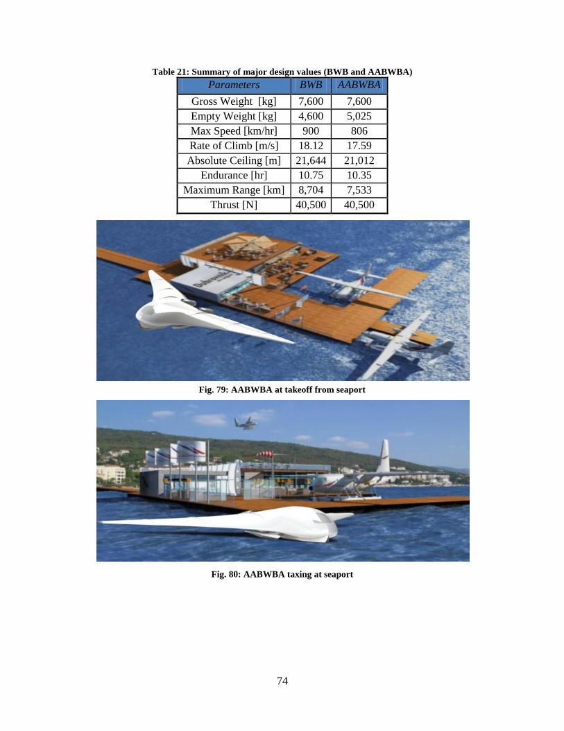
74
Table 21: Summary of major design values (BWB and AABWBA)
Parameters BWB AABWBA
Gross Weight [kg] 7,600 7,600
Empty Weight [kg] 4,600 5,025
Max Speed [km/hr] 900 806
Rate of Climb [m/s] 18.12 17.59
Absolute Ceiling [m] 21,644 21,012
Endurance [hr] 10.75 10.35
Maximum Range [km] 8,704 7,533
Thrust [N] 40,500 40,500
Fig. 79: AABWBA at takeoff from seaport
Fig. 80: AABWBA taxing at seaport

75
6. Conclusions and Recommendations
6.1. Conclusions One of the main purposes of this research was to analyze the optimization and sizing
methodology used in the creation of a preliminary design for an amphibious aircraft and to make
suggestions about ways it can be improved. Of course, it is very difficult to create a perfect
aircraft in every aspect (such as structures, aerodynamics, stability, etc.) analyzed that will then
function perfectly after the first design iteration. The preliminary design aims to locate as many
of the main issues as possible before beginning the detailed design. The optimization design
method, especially on the design of the floating device, proves to be very simple and easy to
handle by the designer, in which time and effort could be saved when deciding the type of
amphibian aircraft to size. The results of the validation work done on the sizing code were very
promising. The geometric parameters predicted by the LOTS were very accurate. The FOTS
sizing code reasonably predicted the size of the floating device, with the largest error in the
predicted performance.
Finally, the preliminary results show some of the advantages of using the trimaran concept
into a seaplane design, and the increase in flight performance when the floats are retracted. For
the flight performance, mounting the floats inside the hull decreases significantly the drag as
compared to an extended position. This increases the flight performance of the seaplane in rate of
climb, range, and endurance, shown in Fig. 55 and Table 15.
The design excels in hydrostatic stability. The trimaran proves to be a stable method as shown
from the FOTS code and the design analysis performed by ORCA 3D. The metacentric height of
this design has a positive value both in the transverse and longitudinal stability. The water speed
that a trimaran shows is also significant, in which water resistance is less compared when using
the wing tip floats or stabilizers as explained by the graph in Fig. 50.
With the help of the design analysis, an extended analysis of the structural strength of the hull
was performed. The analysis shows to have some structural stress on the point where the step is
located. Special attention on this matter has to be addressed. Of course, computer simulations
may prove to be unrealistic and true practical tests are to be made. Finally, ORCA 3D help prove
the theoretical hydrostatic analysis performed by the FOTS code. As well, it was a useful tool in
analyzing wave simulations and finding the maximum heel angle the seaplane must be able to
withstand before overturning. This tool seems useful in analyzing the retractable float system in
water, in which it showed to improve the heel angle 6o when using the float system.
The second aim of this research was to design an “out of the box” idea that stands out not only
because of its improved performance, as well as its unique design idea. On a long term basis, a
brand new seaplane can be designed as well as suitable infrastructure (seaports) in order to
increase seaplane market and operations. The creation of the Blended Wing Body Aircraft
creates a more efficient landplane than a conventional configuration. Combining the advance
trimaran concept to the blended wing body design, an advance amphibian aircraft emerges,
exceeding both water performance and air performance on any kind of amphibian aircraft of its
type. The theoretical design exceeds the “out of the box” thinking, as well as the aesthetic
design. The advance amphibian blended wing body aircraft gets a futuristic design that attracts
the attention of investors, and gets a high social acceptance.
The aim was to keep most of the AABWBA performance as closed to BWB performance.
With the aid of the retracting system, and reducing weight using composite materials, this goal
was possible, in which an overall reduction in flight performance of around 10% was observed
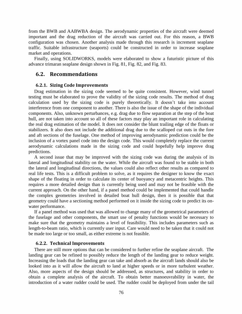
76
from the BWB and AABWBA design. The aerodynamic properties of the aircraft were deemed
important and the drag reduction of the aircraft was carried out. For this reason, a BWB
configuration was chosen. Another analysis made through this research is increment seaplane
traffic. Suitable infrastructure (seaports) could be constructed in order to increase seaplane
market and operations.
Finally, using SOLIDWORKS, models were elaborated to show a futuristic picture of this
advance trimaran seaplane design shown in Fig. 81, Fig. 82, and Fig. 83.
6.2. Recommendations
6.2.1. Sizing Code Improvements
Drag estimation in the sizing code seemed to be quite consistent. However, wind tunnel
testing must be elaborated to prove the validity of the sizing code results. The method of drag
calculation used by the sizing code is purely theoretically. It doesn’t take into account
interference from one component to another. There is also the issue of the shape of the individual
components. Also, unknown perturbances, e.g. drag due to flow separation at the step of the boat
hull, are not taken into account so all of these factors may play an important role in calculating
the real drag estimation of the model. It does not consider the blunt trailing edge of the floats or
stabilizers. It also does not include the additional drag due to the scalloped cut outs in the fore
and aft sections of the fuselage. One method of improving aerodynamic prediction could be the
inclusion of a vortex panel code into the design code. This would completely replace the current
aerodynamic calculations made in the sizing code and could hopefully help improve drag
predictions.
A second issue that may be improved with the sizing code was during the analysis of its
lateral and longitudinal stability on the water. While the aircraft was found to be stable in both
the lateral and longitudinal directions, the values could also reflect other results as compared to
real life tests. This is a difficult problem to solve, as it requires the designer to know the exact
shape of the floating in order to calculate its center of buoyancy and metacentric heights. This
requires a more detailed design than is currently being used and may not be feasible with the
current approach. On the other hand, if a panel method could be implemented that could handle
the complex geometries involved in detailed boat hull design, then it is possible that that
geometry could have a sectioning method performed on it inside the sizing code to predict its on-
water performance.
If a panel method was used that was allowed to change many of the geometrical parameters of
the fuselage and other components, the smart use of penalty functions would be necessary to
make sure that the geometry maintains a level of feasibility. This includes parameters such as
length-to-beam ratio, which is currently user input. Care would need to be taken that it could not
be made too large or too small, as either extreme is not feasible.
6.2.2. Technical Improvements
There are still more options that can be considered to further refine the seaplane aircraft. The
landing gear can be refined to possibly reduce the length of the landing gear to reduce weight.
Increasing the loads that the landing gear can take and absorb as the aircraft lands should also be
looked into as it will allow the aircraft to land at higher speeds or in more turbulent weather.
Also, more aspects of the design should be addressed, as structures, and stability in order to
obtain a complete analysis of the aircraft. To obtain better manoeuvrability in water, the
introduction of a water rudder could be used. The rudder could be deployed from under the tail

77
section of the hull, and retract inside the hull when the seaplane is at flight. Though, this complex
device will increase the empty weight of the seaplane.
Of course, especial attention must be made to the elaboration of the floating devices, and
practical testing must be elaborated to prove the results found from the LOTS and FOTS code
Some improvements done to the BWB design are more specified to the aerodynamics. Wing
twist should be explored to create stall at the root wing before stall occurs at the wing tips. This
will allow the decelerons to remain effective and be in control of the aircraft even if the root
portion of the wings stalls.
To reduce the need to have the elevons always engaged to stabilize the aircraft and balance
the pitching moment of the wings, a reflexive airfoil should be researched and applied to the
aircraft. Although with today’s active and computerized flight control systems, a nonreflexed
airfoil is allowed.
Right now, the BWB has enough space to allow more fuel to be stored onboard without the
need for external fuel tanks. This can greatly increase the endurance of the aircraft and provide
for longer surveillance and scientific monitoring. A system for air refueling should also be
looked into to extend the range and endurance of the aircraft. Since the aircraft can be operated
pilotless; with air refueling, the aircraft can then be operated well over more than ten hours.
The model used to calculate the weight of the wing, fuselage cabin and aft developed by [76]
was sufficient, but more time could be used to refine it for different scaling factors. A better
model for weights would also provide for better CG estimates and a more accurate drag build up.
The BWB was based on the Boeing BWB studies, which were for an 800 passenger aircraft.
A CFD analysis could be performed in the future to verify and validate the designs and models.
In addition, should be given more time, more design variables could have been examined in
LOTS and FOTS to be used as varying parameters in order to find the most suitable HALE BWB
design.
Fig. 81: Futuristic CAD Model of Amphibians at a Modern Sea Port
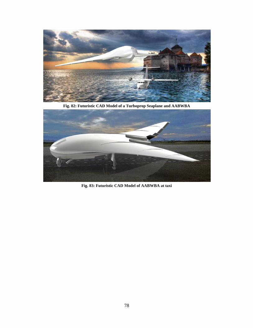
78
Fig. 82: Futuristic CAD Model of a Turboprop Seaplane and AABWBA
Fig. 83: Futuristic CAD Model of AABWBA at taxi

79
References [1] “Design”, (2012) Google search engine [online]; http://dictionary.cambridge.org/search/british/?q=design
[2] Nicolaou, S., “ Flying boats and seaplanes: A history from 1905”, Bay View Books Ltd, 1996
[3] Syed, H., “Amphibian Aircraft Concept Design Study,” Individual Project, University of Glasgow, 2009.
[4] Gunston, B., “World Encyclopedia of Aircraft Manufacturers: From the Pioneers to the Present Day”, 2nd
Edition, The History Press Ltd, 29 Sept 2005
[5] Curtiss, G. H., and Post, A., “The Curtiss Aviation Book”, The Frederick A. Stokes Company, New York, US,
1912
[6] Knott, R., “Flying Boats of the Empire. The Rise and Fall of the Ships of the Sky”, Robert Hale Limited,
London, UK, 2011
[7] “Spruce Goose”, google.com 2012; http://www.theaviationzone.com/factsheets/hk1.asp [Cited Feb 15, 2012]
[8] “Advance Amphibious Vehicles”, google.com 2012; http://www.army-technology.com/projects/efv/ [Cited Mar
13, 2012]
[9] University of New South Wales., “Ekranoplans & Very Fast Craft”, Sydney, Australia, Dec. 1996
[10] Dornier, I., “Mission Dream: Adventures of an aviator”, Airborne Grafix, Dec. 27, 2011
[11] Frawley, G., “The International Directory of Civil Aircraft”, Aerospace Publications, US, 2003
[12] “Beriev” beriev.com 2011; http://www.beriev.com/eng/core_e.html [Cited Jan 26, 2011]
[13] Halirova, J., “Business and Cost Analysis of Seaplanes,” Erasmus Individual Project, Czech Technical
University, Prague, Czech Republic, 2011
[14] Lightening B., “Road Map for Fullfilling Market and Operator Needs in Seaplane Operation within Europe”,
Individual Pilot Feedback Report, Fusetra, 2011.
[15] “Seaplane Facilities,” Seaplane Pilots Association, US Department of Commerce
[16] Canamar, A., Galbraith, R., Gobbi, G., Halirova, J., Smrcek, L., “Long term future opportunities for seaplanes
operations,” FUSETRA Report, Workshop Proceedings & Presentations, University of Glasgow, 2011.
[17] Mohr, B., Schomann, J., “Today’s Seaplane Operations; Results from the 2010 online survey,” FUSETRA
Report, Malta Workshop Proceedings & Presentations, University of Munich, 2010.
[18] Gobbi, G., Canamar, A., “Visionary Concepts for Future European Seaplane Operations,” 3rd
CEAS Air &
Space Conference Paper, University of Glasgow, 2011.
[19] Report of the group of personalities, “European aeronautics: a vision for 2020. Meeting society’ needs and
winning global leadership”, Luxembourg: Office for Official Publications of the European Communities, 2001.
[20] “Seaplane Environmental Impact,” google.com 2011; http://www.seaplanes.org/advocacy/environment.pdf
[Cited Feb 3, 2011]
[21] “Seaplane Environmental Impact” google.com 2011;
http://www.usace.army.mil/environment/Pages/home.aspx [Cited Feb 3, 2011]
[22] Cronin Millar Consulting Engineers, “Seaplane Environmental Impact Information Report,” The Mews Cobh
Co. Cork, 21 Dec 2009
[23] Office for National Statistics, “An investigation into the location and commuting patterns of part-time and full-
time workers in the United Kingdom, using information from the 2001 Census1 Alistair Dent & Stephen Bond”,
Executive Summary, UK, 2008.
[24] Department of Transport, “Public experience of and attitudes towards air travel”, UK, 29th July 2010.
[25] “Aircraft Accidents,” google.com 2011; http://www.aaib.gov.uk/home/index.cfm [Cited Feb 3, 2011]
[26] Transportation Safety Board of Canada, “A Safety Study of Survivability in Seaplane Accidents,” Report
Number SA9401, Canada, 1994.
[27] Raymer, D. P., “Aircraft Design, A Conceptual Approach”, American Institute of Aeronautics and Astronautics,
Inc., Washington D.C., USA, 1992
[28] Smrcek, L., “Aircraft Design for Performance 3” Lecture notes, University of Glasgow, 20011.
[29] “Dornier Do.228” google.com 2011; http://www.raf.mod.uk/equipment/islander.cfm [Cited Jan 26, 2011]
[30] “Britten Norman BN 2” google.com 2011; http://www.raf.mod.uk/equipment/islander.cfm [Cited Jan 26, 2011]
[31] “BAe 146” baesystems.com 2011;
http://www.baesystems.com/Newsroom/NewsReleases/2009/autoGen_10903093820.html [Cited Jan 26, 2011]
[32] “Antonov AN-72” aerospaceweb.org 2011; http://www.aerospaceweb.org/aircraft/transport-m/an72/ [Cited Feb
2, 2011]
[33] Taylor, J., Allen, J.E., Smith, A.G., “Flight Investigations of Some Airworthiness problems of Civil Boat
Seaplanes”, Ministry of Supply, Aeronautical research Council Reports and Memoranda, 1958.
80
[34] “Seaplane Design Features,” Quest for Performance: The Evolution of Modern Aircraft,
http://www.hq.nasa.gov/pao/History/SP-468/ch8-2.htm [retrieved 15 May 2011].
[35] Tomaszewski, K. M., “Hydrodynamic Design of Seaplanes.” A.R.C. Technical Report. Ministry of Supply.
Aeronautical Research Council. London, United Kingdom, 1950.
[36] Vargas, F., “Concept Design of Seaplane Floats”, Individual Dissertation Project, University of Glasgow, 2011
[37] Benson, J., Bidwell J., “Bibliography and Review of Information relating to the Hydrodynamics of Seaplanes”,
NACA Advance Confidential Wartime Report, 1945
[38] Dathe, I., “Hydrodynamic Characteristics of Seaplanes as Affected by Hull Shape Parameters,” A.I.A.A.
Advance Marine Vehicles Journal, United States of America, 1989.
[39] Fletcher, G. L., Llewelyn-Davies, D. I., “Note on Some Tank Tests on the Sunderland III for Takeoff at Extreme
Overload”, British R.A.E. Report, Aero 1887, UK, 1943.
[40] Davis B., W., “Analysis of Results - Hydrodynamic Research Project”, Boeing Aircraft Company, Rep. No. D-
5558, USA, 1944.
[41] Brimm, D. J., “Seaplanes: Maneuvering, Maintaining, Operating”, Pitman Publishing Corporation, New York,
NY, 1937.
[42] Langley, M., “Seaplane Float and Hull Design”, Sir Isaac Pitman & Sons, LTD, London, UK, 1935.
[43] Garner, H. M., Coombes, L. P., “Seaplane Hulls and Floats: An Epitome of Present Knowledge with
Suggestions for Future Research,” Aircraft Engineering and Aerospace Technology, Vol. 2, No. 9, 1930, pp.
221-225.
[44] Munro, W., “Marine Aircraft Design”, Sir Isaac Pitman & Sons, LTD., London, 1933
[45] Nelson, W., “Seaplane Design”, 1st ed. McGraw-Hill Book Company, Inc., New York, NY, 1934.
[46] Carter, A. W., “Recent N.A.C.A. Research on High Length-Beam Ratio Hulls,” Journal of the Aeronautical
Sciences, Vol. 17, No. 3, 1949, pp. 167-183.
[47] Benson, J. K., Lina, L. J., “The Use of a Retractable Planning Flap Instead of a Fixed Step on a Seaplane,”
NACA L-257, 1943.
[48] Mottard, E. J., “A Brief Investigation of the Effect of Waves on the Take-Off Resistance of a Seaplane,” NASA
TN-D-165, 1959.
[49] Jenkinson, L. R., Marchman, J. F., 1993, “Aircraft design projects: for engineering students”, American
Institute of Aeronautics and Astronautics, Inc.; Oxford: Butterworth-Heinemann, Reston, VA, 1993.
[50] Klemin, A., Pierson, J.D., Storer, E. M., “An Introduction to Seaplane Porpoising,” Journal of the Aeronautical
Sciences, Vol. 6, No. 8, 1939, pp. 311-318.
[51] Smith, A.G., White H. G., “A review of Porpoising Instability of Seaplanes,” A.R.C. Technical Report. Ministry
of Supply. Aeronautical Research Council. London, United Kingdom, 1954
[52] Vagianos, N. J., Thurston, D. B., “Hydrofoil Seaplane Design,” Thurston Aircraft Corp., Rept. to Department of
the Navy Air Systems Command, Sanford, ME, 1970.
[53] “The Hydrofoil and Float Combination,” Seaplane Pilots Association, Aug. 2008,
http://www.seaplanes.org/mambo/index.php?option=com_content&task=view&id=221&Itemid=245 [retrieved
20 June 2011].
[54] Wood, R., “Performance Multihulls Part 1 and 2”, Multihull Review Magazine, UK, 2007.
[55] Brown, J., “The Case for the Cruising Trimaran”, BookSpecs Publishing, Pennsville, NJ 08070, USA, 2010.
[56] Mohanty, P., “Concept Design of Seaplane Hulls”, Individual Dissertation Project, Aerospace Engineering,
University of Glasgow, 2011
[57] Bertorello, C., Bruzzone, D., Cassella, P., Zotti, I. “Trimaran Model Test Results and Comparison with
Different High Speed Craft.” Elsevier Science Ltd. Italy, 2001.
[58] Begovic, E., Bertorello, C., Cassela, P., “Calm Water Experimental Research On Geosims Of High Speed
Trimaran Hydrodynamic Characteristics And Model-Ship Correlation”, Practical Design of ships and other
floating structures, Elsevier Science limited, 2001.
[59] “Retractable Floats”, google.com 2011; http://www.tigerfishaviation.net/ [Cited April 21, 2011]
[60] Raymer, D. P., “Aircraft Design, A Conceptual Approach”, Chapter XII “Aerodynamics”, page 285, American
Institute of Aeronautics and Astronautics, Inc., Washington D.C., USA, 1992
[61] Raymer, D. P., “Aircraft Design, A Conceptual Approach”, Chapter XV “Weights”, page 395, American
Institute of Aeronautics and Astronautics, Inc., Washington D.C., USA, 1992.
[62] Bradley, K. R., “A sizing methodology for the conceptual design of blended-wing-body transports”. CR 2004-
213016, NASA, September 2004.
[63] Schaufele, R. D., “The Elements of Aircraft Preliminary Design”. Aries Publications, 2000.

81
[64] Langley, M., “Seaplane Float and Hull Design”, Chapter IV “Float Design”, page 65, Sir Isaac Pitman &
Sons, LTD, London, UK, 1935.
[65] Parkinson, J. B., “Design Criterions for the Dimensions of the Forebody of a Long-Range Flying Boat,”
Wartime Report 3K08. National Advisory Committee for Aeronautics, Washington, USA, 1943
[66] “Main Float Buoyancy,” FAR 23.751, Federal Aviation Administration, 2011.
[67] Comstock, J., “Principles of Naval Architecture.” New York: Society of Naval Architects and Marine
Engineers. 1967.
[68] Wells, V., “Review of Aircraft Aerodynamics,” Course Notes, Dept of Aerospace Engineering, Arizona State
University, 2008.
[69] Sederberg, M. T., Sederberg, T. W., “T-Splines: A Technology for Marine Design with Minimal Control
Points”, Chesapeake Powerboat Symposium, Annapolis, MD, March 2010.
[70] Dahlmo Kl Andersson M., Gellerstedt M., and Karlsson S., “Methods to assess the accuracy of a CAD
program,” Nobel Biocare, S-402 26 Goteborg, Sweden.
[71] “Industries using SOLIDWORKS,” google.com 2013 http://www.solidworks.com/sw/successes/overview-
results.htm [Cited Feb. 19, 2013]
[72] Amihan, C., Chen E., Nadzakovic, Z., Pickering, R., “The High-Altitude, Long Endurance, Blended Wing
Body” Final Year Project, Dept of Aerospace Engineering, Arizona State University, 2010
[73] Callaghan, J. T., and Liebeck, R. H., “Some thoughts on the design of subsonic aircraft for the 21st century”.
SAE Paper No. 901987, October 1990.
[74] Liebeck, R. H., Page, M. A., Rawdon, B. K., Scott, P. W., and W. R. A. “Concepts for advanced subsonic
transports”. CR 4624, NASA, September 1994.
[75] Ko, Y. A. “The Multidisciplinary Design Optimization of a Distributed Propulsion Blended-Wing-Body
Aircraft”. PhD thesis, Virginia Tech, Blacksburg, VA., April 2003.
[76] Bradley, K. R., “A sizing methodology for the conceptual design of blended-wing-body transports”. CR 2004-
213016, NASA, September 2004.
[77] Jedlicka,L., “Seaplane Conversion Artistic Images,” UG student of VSVU Bratislava (Slovakia)

82
Appendix
Appendix A. Empirical Equations
A.1 Empty Weight Breakdown Equations
A.1.1. Structures Wing For composites ff = 0.6528, else ff = 0.768. Value of 0.768 is a multiplicative factor for flying wings.
(
)
( )
(A.1.1)
where ff=Fudge Factors, Nz=Ultimate Load Factor; =1.5x limit load factor, t=Wing Thickness, Sw=Trapezoidal Wing
Area, Wfw=Weight of Fuel in Wing.
Fuselage For a conventional aircraft the equation for the weight of the fuselage is as follows. For advanced
composites ff = 0.9, else ff = 1.
[ ( )
( ⁄ )
] (A.1.2)
( ) (A.1.3)
where Sf=Fuselage Wetted Area, Lt=Tail Length, Lf=Total Fuselage Length, d=Fuselage Structural Depth,
Wpress=Weight Penalty due to Pressurization, Vpr=Volume of Pressurized Section, =Pressure Difference
Centerbody For a Blended Wing Body (BWB) aircraft, the fuselage or centerbody is split into two sections, the
crew cabin and the aft section, in order to predict the weight accurately.
Cabin The weight of the BWB cabin is taken from [62], who derived the equation from the weight equation of a
cigar shaped fuselage.
(A.1.4)
where Scabin=Cabin Wetted Area.
Aft Eq. (A.1.5), also taken from [62], estimates the weight of the aft section as if it were a horizontal tail, but
with modifications in the equation to include engine placement.
( ) ( ) (A.1.5)
where Nen =Number of engines, Saft=Fuselage Aft Area
Horizontal Tail For advanced composites ff = 0.83, else ff = 1.
( )
( ⁄
)
(
)
(A.1.6)
where t=Wing thickness.
Vertical Tail For advanced composites ff = 0.83, else ff = 1.
( ) ( )
(
⁄
)
(
)
(A.1.7)
where Ht=Horizontal Tail Height above Fuselage, Hv=Vertical Tail Height above Fuselage
. Landing Gear ff = 0.95 for advanced composites for both landing gear types.
Main Landing Gear (MLG)

83
( ) (
)
(A.1.8)
Nose Landing Gear (NLG)
( ) (
)
(A.1.9)
where Nl=Ultimate Landing Load Factor, GWL=Landing Design Gross Weight, Lm=Length of Main Landing Gear,
Ln=Length of Nose Landing Gear.
A.1.2. Propulsion Engine
(A.1.10)
Fuel System
(
⁄)
(A.1.11)
where Wen=Engine Weight, Vt=Total Fuel Volume, Vi=Integral Tanks Volume, Nt=Number of Fuel Tanks
A.1.3. Equipment Flight Control
(
) (A.1.12)
Hydraulics
(A.1.13)
Avionics
(A.1.14)
Electrical
( ) (A.1.15)
Anti-Ice System
(A.1.16)
where WUAV=Uninstalled Avionics Weight
A.2 Flat Plate Drag Area Breakdown Equations In addition to lift, the wing and body traveling through the air generates drag. The drag consists of viscous or
parasite drag as well as lift-induced drag. Most aircraft today travel fast enough that they also have an additional
drag arising from compressibility effects.
A useful measure of the parasite drag is the equivalent flat plate-drag area, f. Therefore, the total parasite drag is:
(A.2.1)
To calculate f is done by doing a drag component buildup. Each exterior component of the airplane is considered
separately, and the f of each component is found. The total f of each component is finally sum together of all the
drag areas. The equivalent flat plate drag area can be computed from the following expression:
(A.2.2)
Where Cf is the friction coefficient, F is the form factor, Q is the interference factor, and Swet is the wetter Area.
Friction coefficient depends on the Reynolds number and the surface roughness, and is affected whether the flow
is laminar or turbulent. Friction coefficient can be computed by the following expression:
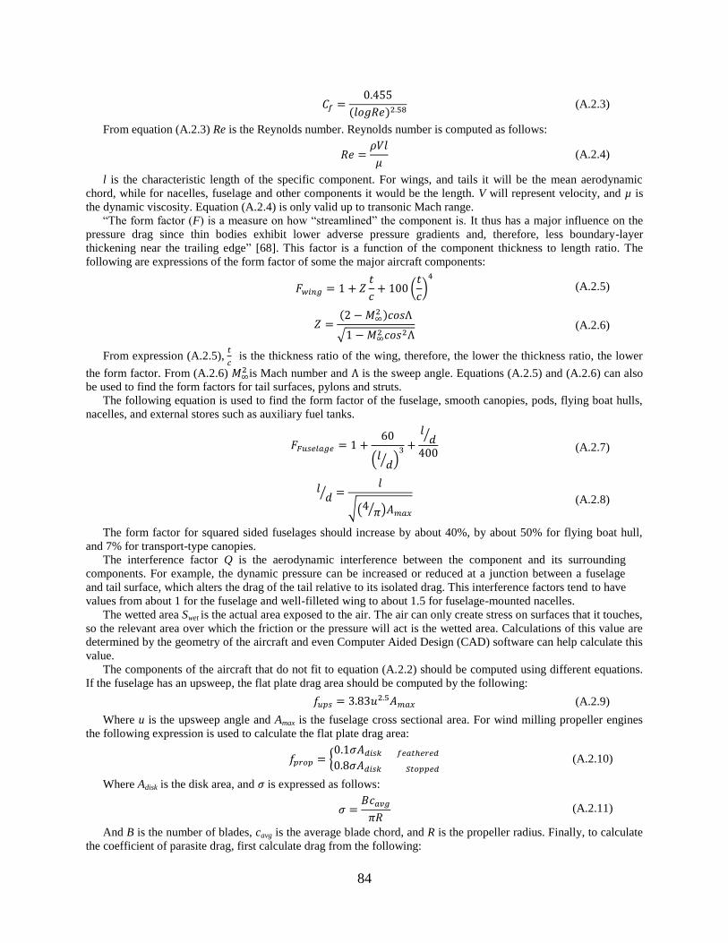
84
( ) (A.2.3)
From equation (A.2.3) Re is the Reynolds number. Reynolds number is computed as follows:
(A.2.4)
l is the characteristic length of the specific component. For wings, and tails it will be the mean aerodynamic
chord, while for nacelles, fuselage and other components it would be the length. V will represent velocity, and µ is
the dynamic viscosity. Equation (A.2.4) is only valid up to transonic Mach range.
“The form factor (F) is a measure on how “streamlined” the component is. It thus has a major influence on the
pressure drag since thin bodies exhibit lower adverse pressure gradients and, therefore, less boundary-layer
thickening near the trailing edge” [68]. This factor is a function of the component thickness to length ratio. The
following are expressions of the form factor of some the major aircraft components:
(
)
(A.2.5)
(
)
√
(A.2.6)
From expression (A.2.5),
is the thickness ratio of the wing, therefore, the lower the thickness ratio, the lower
the form factor. From (A.2.6) is Mach number and is the sweep angle. Equations (A.2.5) and (A.2.6) can also
be used to find the form factors for tail surfaces, pylons and struts.
The following equation is used to find the form factor of the fuselage, smooth canopies, pods, flying boat hulls,
nacelles, and external stores such as auxiliary fuel tanks.
( ⁄ )
⁄
(A.2.7)
⁄
√( ⁄ )
(A.2.8)
The form factor for squared sided fuselages should increase by about 40%, by about 50% for flying boat hull,
and 7% for transport-type canopies.
The interference factor Q is the aerodynamic interference between the component and its surrounding
components. For example, the dynamic pressure can be increased or reduced at a junction between a fuselage
and tail surface, which alters the drag of the tail relative to its isolated drag. This interference factors tend to have
values from about 1 for the fuselage and well-filleted wing to about 1.5 for fuselage-mounted nacelles.
The wetted area Swet is the actual area exposed to the air. The air can only create stress on surfaces that it touches,
so the relevant area over which the friction or the pressure will act is the wetted area. Calculations of this value are
determined by the geometry of the aircraft and even Computer Aided Design (CAD) software can help calculate this
value.
The components of the aircraft that do not fit to equation (A.2.2) should be computed using different equations.
If the fuselage has an upsweep, the flat plate drag area should be computed by the following:
(A.2.9)
Where u is the upsweep angle and Amax is the fuselage cross sectional area. For wind milling propeller engines
the following expression is used to calculate the flat plate drag area:
{
(A.2.10)
Where Adisk is the disk area, and is expressed as follows:
(A.2.11)
And B is the number of blades, cavg is the average blade chord, and R is the propeller radius. Finally, to calculate
the coefficient of parasite drag, first calculate drag from the following:

85
(A.2.12)
Then replacing equation (A.2.12) to (A.2.1) and deriving the coefficient of drag the following is obtained:
(A.2.13)
So the total flat plate drag area depends on the wing area. So as the wing area increases, parasite drag decreases.
But as the flat plate drag area increases, parasite drag increases.
A.3 Aircraft Flight Performance Equations The performance of an aircraft is important parameters that are calculated in order to compare the aircraft with
other competitors and to evaluate the whole aircraft performance in the conceptual design. So the computations that
were done in this project for the performance of this aircraft is required thrust and power, level flight airspeed, total
time of flight on take-off, climb, cruise, descent and landing, endurance and range and finally steady level turns.
Equation (A.3.1) is the expression for lift coefficient.
(A.3.1)
To calculate the minimum or stall speed the following expression is utilized:
√
(A.3.2)
To calculate the equivalent airspeed is as follows:
√ (A.3.3)
(A.3.4)
To calculate the service and absolute ceiling of an aircraft is necessary to calculate the climb speed, climb angle
and the climb gradient. The following shows the equations for climb speed, climb angle and climb gradient,
respectively:
( )
( )
(A.3.5)
(
) (
) (A.3.6)
( ) (A.3.7)
Where TA and PA are the thrust available and power available generated by the engines of the aircraft. Another
important parameter of the climb section useful in the performance of an aircraft is the time and distance climb. The
following equations are useful to calculate the time and distance of climb:
∫
( ) ̃
(A.3.8)
∫ ( )
(A.3.9)
For aircraft with low power to weight ratio it can be assumed that ( ) . Therefore, (A.3.9) is derived as
follows:
∫
(A.3.10)
Finally, with the climb speeds of the aircraft the absolute and service ceiling can be calculated. Same rules apply
for the descent characteristics of the aircraft, however using different equations. Since the aircraft is not descending
at a perfect vertical line, an angle of descent must be added to calculate the lift coefficient at descent. The following
equation is used:

86
( ) (A.3.11)
The angle of descent can be established by the aircraft to calculate the required thrust or it can be calculated by
the following derivation:
(
) (
) (
) (A.3.12)
Where VD is the speed of descent and Vx is the horizontal speed and are derived from the following expressions:
(A.3.13)
(A.3.14)
where
(
)
√
(A.3.15)
To calculate the required thrust Newton’s second law is applied, where:
(A.3.16)
Deriving TR and simplifying Drag (D), the following is obtained:
(A.3.17)
The same equations to calculate the time of descent and distance of descent (A.3.8) and A.3.10) apply as in the
climb section, however changing the climb speed to speed of descent.
Two other aspects that are calculated on the flying segment of an aircraft are the take-off and landing. Most
aircraft required large amounts of thrust in order to perform the required take-off specify by the aviation authorities.
So to calculate the required thrust for the aircraft to perform the take-off segment, it must be calculated the
acceleration. The acceleration will be divided on the ground run, and acceleration on air. To calculate acceleration
on ground, Applying Newton’s Second Law, the following is obtained:
( )
(A.3.18)
Where Ta is the thrust available, D is Drag Force and F is the Gear drag or Friction Force. To calculate F the
following is used:
( ) (A.3.19)
µ is the friction coefficient. When the aircraft is at the air, F is removed from equation (A.3.18):
( )
(A.3.21)
With the acceleration of the aircraft on both on the ground run and air, the time and distance to take-off can be
calculated. This time will be calculated until the aircraft reaches lift-off speed before it starts the transition arc. To
calculate the lift-off speed (VLOF) and take-off safety speed (Vr) the following is used:
(A.3.22)
(A.3.23)
Then to calculate the distance of take-off until the aircraft reaches take-off safety speed is as follows:
(A.3.24)
( )
(A.3.25)
and finally to calculate the real time speed necessary to calculate the distance, since
, deriving from this
expression:
(A.3.26)
(A.3.27)

87
So this method of calculation requires loop iterations where acceleration depends on Lift, and Drag Force; Lift and
Drag Force requires speed; and speed depends on acceleration.
So after the aircraft had reached take-off safety speed (Vr), the aircraft must perform a transition arc, in which a lift
load factor is required. With the lift load factor calculated, the radius of transition arc, the angle of climb, the length
of transition arc, the increment of altitude and the time of transition arc are derived by the following, respectively:
(
)
(A.3.28)
( ) (A.3.29)
(
) (A.3.30)
(A.3.31)
( ) (A.3.32)
(A.3.33)
Finally for the final climb up to 10.5 m (35ft), the following equations to calculate the length of climb and time of
climb are used:
(A.3.34)
(A.3.35)
For the landing segment, the same iteration loop that is used to calculate the take-off segment is also applied. First
the available speed and the touchdown speed should be calculated:
(A.3.36)
(A.3.37)
Therefore, first the descent from altitude of 15m (50ft) must be calculated. So using equations (A.3.34) and
(A.3.35) the initial length of climb and time are calculated, where h3 will be from (A.3.32) and r will come from
(A.3.29). The only difference to the equations above will be replacing VLOF with VA. The same will be apply to the
transition arc segment at landing, however a new airspeed at the end of the arc must be calculated and an end time
using the following derivations:
√ (A.3.38)
( ) (A.3.39)
So for the deceleration on the air and ground same rule applies as in the take-off segment. However, the
acceleration will be calculated differently. Since no thrust is required at landing and the drag force will act in the
opposite side, a new derivation for the acceleration (deceleration) on the air is being calculated:
( )
(A.3.40)
As the aircraft touches the ground, the acceleration force will add the gear drag and the following is applied:
( )
(A.3.41)
where (A.3.42)
and ( ) ( )
(A.3.43)

88
(A.3.44)
Ff stands for force on front gear, Fm is the force on the main gears, XG is the horizontal arm of centre of gravity, YG
is the vertical arm of centre of gravity, XF is the horizontal arm of front gear, µf is the friction coefficient when no
brakes are applied and µm is the friction coefficient when brakes are applied. After the acceleration is calculated, the
speed is calculated using equation (A.3.27), and finally the distance is calculated until the aircraft reaches 0 speed
using equation (A.3.25).
Calculating the performance time and distance of take-off, climb, descent, and landing, it can be calculated the
cruise time and distance using the maximum fuel capacity the aircraft can carry. From equation (11) the fuel for
level flight is calculated using the following:
(A.3.45)
Where mf is the total mass of the fuel, L is level flight, Taxi is fuel at taxi segment, TO stands for take-off, C is
climb, D is for descent, LN is for landing, and H is for holding fuel or fuel reserve. To calculate the mass of the fuel
for each segment the following equation is used:
(A.3.46)
ti is the total time of each flight segment and FChr is the Fuel consumption per hour derived from the following:
(A.3.47)
SFC is the specific fuel consumption and P is the shaft power of the engine. Engines have different ratings in
which the engine can be operating depending on the flight segment; maximum contingency, maximum take-off,
maximum continuous, and idle. At take-off the engines operate at maximum take-off, at climb and level flight
engines are operating at maximum continuous rating, and for descent and landing engines operate at idle rating.
Once the mass of the fuel at level flight is calculated using equation (A.3.45), the time of flight can be calculated
using equation (A.3.46). The distance at level flight is computed from the following:
(A.3.48)
The sum of the all the distance segments will give the range of the aircraft. Finally, another aspect of the
performance of the aircraft that can be calculated is the steady level turns. This is obtained if the available thrust
equals the required thrust, expressed as followed:
(A.3.49)
A.4 Hull geometrical empirical formulas Bow Height:
(A.4.1)
Step Height:
(A.4.2)
Flat forebody length:
(A.4.3)
Chine Flare Length:
(A.4.4)

89
Appendix B. Artistic impressions of the conversion of current certified
aircraft to a seaplane The following images are an impression of the artist of some certified aircraft that could be converted into a
seaplane [77]. The characteristics of this aircrafts are shown in Table 2.
Fig. 84: Artistic Impression of LET L-410 [77]
Fig. 85: Artistic Impression of Antonov AN28 [77]
Fig. 86: Artistic Impression of BAE 146 [77]
Fig. 87: Artistic Impression of Dornier DO-228 [77]

90
Appendix C. MATLAB Optimization Source Code %% Floating Device Optimized Testing Source Code %% %%% by Alan Canamar %%% clc; clear all
%% Input Parameters
global GW g0 rho0 rhos ... Sexp2 CLmax0 d L
prompt = {'Enter Maximum Takeoff Weight [kg]:',... 'Enter Main Landing Gear Weight [kg]:',... 'Enter Nose Landing Gear Weight [kg]:','Enter Empty Weight [kg]:',... 'Enter Maximum Fuel Weight [kg]:','Enter Maximum Payload Weight
[kg]:',... 'Enter Wing Area [m^2]:','Enter Fuselage Diameter [m]:'}; prompt2 = {'Enter Fuselage Length [m]:','Enter Wing Span [m]:',... 'Enter Maximum Lift Coefficient:','Enter Plate Drag Breakdown [m^2]:',... 'Enter Cruising Speed [km/hr]:','Enter Cruising Altitude [m]:',... 'Enter Center of Gravity of Landplane from Bottom [m]:',... 'Enter Thrust Available of Aircraft [N]:'}; dlg_title = 'Input Initial Aircraft Parameters'; num_lines = 1; def = {'7600','80','70','4600','1550','1850','39.02','2.4'}; def2 = {'13.69','23.47','1.3','0.445','900','12200','0.7','40500'}; C = inputdlg(prompt,dlg_title,num_lines,def); C2 = inputdlg(prompt2,dlg_title,num_lines,def2); GW = str2double(C(1,1)); %Maximum Takeoff Weight [kg] MLG = str2double(C(2,1)); %Main Landing Gear Weight [kg] NLG = str2double(C(3,1)); %Nose Landing Gear Weight [kg] EW = str2double(C(4,1)); %Empty Weight [kg] MF = str2double(C(5,1)); %Maximum Weight of Fuel [kg] Wpay = str2double(C(6,1)); %Maximum Payload Weight [kg] Sexp2 = str2double(C(7,1)); %Wing Area [m^2] d = str2double(C(8,1)); %Diameter of Fuselage [m] L = str2double(C2(1,1)); %Length of Fuselage [m] b2 = str2double(C2(2,1)); %Wing Span [m] CLmax0 = str2double(C2(3,1)); %Maximum Lift Coefficient of the Wing ftotal_air = str2double(C2(4,1));%Aircraft Flat Plate Breakdown [m^2] Vel = str2double(C2(5,1)); %Cruising speed [km/hr] ALT = str2double(C2(6,1)); %Cruising altitude [m] CGL = str2double(C2(7,1)); %Center of Gravity [m] TA = str2double(C2(8,1)); %Thrust Available [N]
%% Global Inputs rhow = 1000; %Density of Water [kg/m^3] rhos = 1025; %Average Density of Salt Water [kg/m^3] g0 = 9.80665; %Gravitational Constant [m/s^2] rho0 = 1.225; %Density of air at Sea Level [kg/m^3]
%% WEIGHTS %Weight of Langing Gear WLG = MLG+NLG;
%Total Gross Weight with no Landing Gear [kg]

91
GW0 = GW - WLG;
%Weight of Boat Hull [kg] Wb = round(GW0*0.12); %Aluminum Material Wbc = round(GW0*0.03); %Composite Materials
%Weight of Floats [kg] nf = 2; %Total number of floats if nf == 0; Wft = 0; else Wf = round(GW0*0.02); Wft = Wf*nf; %Total Weight of floats [kg] end Wftc = round(Wft*0.5); %Composite Materials
%Weight of Mid Wing Stabilizers [kg] nMW = 2; %Total number of stabilizers if nMW == 0; WMW = 0; else WMW = round(GW*0.02); WMW = WMW*nMW; %Total Weight of stabilizers [kg] end WMWc = round(WMW*0.5); %Composite Materials
%Weight of Wing Tip Stabilizers [kg] nWT = 2; %Total number of stabilizers if nWT == 0; WWT = 0; else WWT = round(GW*0.012); WWT = WWT*nWT; %Total Weight of stabilizers [kg] end WWTc = round(WWT*0.5); %Composite Materials
%Total Empty Weight Seaplane with Floats, Boat Hull [kg] EWt = EW+Wb+Wft; %Aluminum Material EWc = EW+Wbc+Wftc+50; %Composite Materials
%Total Empty Weight Seaplane with Mid Wing, Boat Hull [kg] EWMt = EW+Wb+WMW; %Aluminum Material EWMc = EW+Wbc+WMWc; %Composite Materials
%Total Empty Weight Seaplane with Wing Tip, Boat Hull [kg] EWWTt = EW+Wb+WWT; %Aluminum Material EWWTc = EW+Wbc+WWTc; %Composite Materials
%Reduced Payload Weight, Using Max Fuel [kg] WPa = GW - EW - MF; %Landplane WPs = GW - EWt - MF; %Aluminum Seaplane WPsc = GW - EWc - MF; %Composite Seaplane
%Reduced Fuel Weight, Using Max Payload [kg] WFa = GW - EW - Wpay; %Landplane

92
WFs = GW - EWt - Wpay; %Aluminum Seaplane WFsc = GW - EWc - Wpay; %Composite Seaplane
%% Trimaran Dimensions [b,Lh,bo,Lo,y,h,ho] = Trimaran_Dimensions();
%% Stabilizer Dimensions [bstab,Lstab,dstab,l,VF1] = Stabilizer_Dimensions(CGL);
%% WingTip Floats Dimensions [bstabWT,LstabWT,dstabWT,VFWT1] = Wingtip_Dimensions(CGL,b2);
%% Hydrostatics of Seaplane [GMS,GMSy,Dras] = Hydrostatics(b,Lh,h,bo,Lo,ho,y,CGL,b2,bstab,Lstab,dstab,... l,bstabWT,LstabWT,dstabWT,VF1,VFWT1);
%% Water Loads [a] = WaterLoads(b,Dras);
%% Drag Curves [DPi,DPis] = Drag_Curves(L,b2,d,b,Lh,bo,Lo,TA,ALT);
%% Aerodynamic Drag Comparison [Cd,Cdsi,Cdsie,ftotal_air] = Aero_Drag(Lh,b,Lo,bo,Vel,ALT);
%% Aircraft Drag [Cd,D] = Aircraft_Drag(ftotal_air,b2,Vel,ALT);
%% Seaplane Drag Increase [Cdsi,Cdsie,Cdsist,Cdsiest,CdsiWT,CdsieWT] = Seaplane_Drag(Lh,b,Lo,bo,... bstab,Lstab,bstabWT,LstabWT,Vel,ALT);
%% Water Performance [FTm,Rw] = Water_Resistance(Lh,Lo,b,h,bo,ho,Lstab,bstab,... dstab,bstabWT,LstabWT,dstabWT,VF1,VFWT1,TA,CLmax0,ALT);
%% Flight Performance TurboProp Engine [Ttotal,Ltotal,Ttotalse,Ltotalse,Vmax,Vmaxs] = Flight_Performance... (EW,EWc,MF,Wpay,Cd,Cdsi,Cdsie,Lh,Lo,b,bo,TA,ALT,Vel);
%% Flight Performance JET Engine [Ttotalj,Ltotalj,Ttotalsej,Ltotalsej,Vmax,Vmaxs] = Flight_Performance_JET... (EW,EWc,MF,Wpay,Cd,Cdsi,Cdsie,Lh,Lo,b,bo,TA,ALT,Vel);
%% Gust Envelope [Vstall] = Gust(ALT,Vel);
%% Results fprintf('-----------------------------------------------------') fprintf('\n Weight Parameters\n') fprintf('\n Total Gross Weight no Landing Gear [kg] = %g\n', GW0) fprintf('\n Total Weight of Floats [kg] = %g\n', Wftc) fprintf('\n Total Weight of Boat Hull [kg] = %g\n', Wbc) fprintf('\n Total Weight of Stabilizers [kg] = %g\n', WMWc)

93
fprintf('\n Total Weight of Wing Tip Floats [kg] = %g\n', WWTc) fprintf('\n Empty Weight of Seaplane Trimaran [kg] = %g\n', EWc) fprintf('\n Empty Weight of Seaplane Mid Wing [kg] = %g\n', EWMc) fprintf('\n Empty Weight of Seaplane Wing Tip [kg] = %g\n', EWWTc) fprintf('\n Payload Weight of Seaplane w/Max Fuel [kg] = %g\n', WPsc) fprintf('\n Fuel Weight of Seaplane w/Max Payload [kg] = %g\n', WFsc) fprintf('\n-----------------------------------------------------\n') %% Sizing Trimaran Geometry Code Created by Alan Canamar %%
function [b,Lh,bo,Lo,y,h,ho] = Trimaran_Dimensions() %% Declare global variables global GW rhos L
%% Trimaran Dimensions % clc; clear all % GW = 6600; %Total Gross Weight of Aircraft [kg] % rhos = 1025; %Density of Salt Water [kg/m^3] % L = 14.47; %Length of Fuselage [m] % CGL = 1.594; %Landplane Centre of Gravity [m] % b2 = 19.08; %Wingspan [m] BouyR = 1.9; %Bouyancy Reserve [Percent] HullR = 1.5; %Hull Displacement [Percent] OutR = BouyR - HullR; %Outrigger Displacement [Percent] delT = BouyR*GW; %Aircraft Total Displacement on Water [kg] delb = HullR*GW; %Boat Hull Total Displacement [kg] del0 = OutR*GW; %Outriggers Total Displacement [kg] del1 = del0/2; %Displacement on one Outrigger [kg]
%% Boat Hull Design lf_lah = 2.07; %Afterbody Forebody Ratio [Percent] Bhh = 0.65; %Bow height increment [Percent] Shh = 0.09; %Step Height increment [Percent] chh = 0.08; %Chine Flare increment [Percent] Lch = 1.7; %Flat Forebody increment [Percent] V = delb./rhos; %Displacement Volume [m^3] Lh = Inf; %Length [m] SLR = 20; %Slenderness Ratio precision = 0.01; precisionK = 0.0001; minK = 0.0525; maxK = 0.0975; matK = [(minK:precisionK:maxK)', Inf(length(minK:precisionK:maxK),1),... Inf(length(minK:precisionK:maxK),1),... Inf(length(minK:precisionK:maxK),1)]; i = 1; for K = minK:precisionK:maxK while Lh > L Lf_b = SLR/lf_lah; %Forebody Ratio Cv0 = K*Lf_b^2; %Static Load Coefficient b = (delb/(rhos*Cv0))^(1/3);%Beam Width [m] Lh = SLR*b; %Length [m] Lhf = (1/lf_lah)*L; %Forebody Length [m] Lha = L-Lhf; %Afterbody Length [m] h = b*Bhh; %Bow Height [m] S = b*Shh; %Step Height [m]

94
ch = b*chh; %Chine Flare [m] Lc = b*Lch; %Flat Forebody Length [m] if Lh > L SLR = SLR - precision; end end matK(i,2) = SLR; matK(i,3) = Lh; matK(i,4) = b; i=i+1; Lh = Inf; SLR = 20; end
%Calculations for Boat Hull [SLR, idx] = max(matK(:,2)); K = matK(idx,1); Lf_b = SLR/lf_lah; %Forebody_beam Ratio Cv0 = K*Lf_b^2; %Static Load Coefficient b = (delb/(rhos*Cv0))^(1/3);%Beam Width [m] Lh = SLR*b; %Length [m] Lhf = (1/lf_lah)*Lh; %Forebody Length [m] Lha = Lh-Lhf; %Afterbody Length [m] h = b*Bhh; %Bow Height [m] S = b*Shh; %Step Height [m] ch = b*chh; %Chine Flare [m] Lc = b*Lch; %Flat Forebody Length [m] Vha = (0.45)*Lh*b*h; %Actual Volume [m^3] disp(' ') if V <= Vha fprintf('Hull = Pass'); else fprintf('Hull = Fail'); end
%% Outrigger Design part 2 Lb = 14; %Length to Beam Ratio k = 0.08; %Spray Coefficient L_Lo = 0.4925; %Outrigger to Hull Length ratio lf_lao = 2.11; %Afterbody_Forebody Ratio [Percent] Bho = 0.9; %Bow height increment [Percent] Sho = 0.09; %Step Height increment [Percent] chho = 0.08; %Chine Flare increment [Percent] lco = 1.7; %Flat Forebody increment [Percent] Vo = del1./rhos; %Displacement Volume [m^3] Lo = L_Lo*Lh; %Length [m] bo = Lo/Lb; %Beam width [m] lf = Lo/lf_lao; %Forebody Length [m] la = Lo-lf; %Afterbody Length [m] ho = bo*Bho; %Bow Height [m] Sh = bo*Sho; %Step Height [m] cho = bo*chho; %Chine Flare [m] lc = bo*lco; %Flat Forebody Length [m] y = Lh*0.12; %Y displacement of Outrigger from main Hull [m] x = Lh*(-0.0625); %X displacement of Outrigger from main Hull [m] Voa = (1/2)*Lo*bo*ho; %Actual Volume [m^3]

95
disp(' ') if Vo <= Voa fprintf('Outrigger = Pass'); else fprintf('Outrigger = Fail'); end disp(' ')
%% Results fprintf('-----------------------------------------------------') fprintf('\n Dimensional Parameters\n') fprintf('\n Boat Hull Dimensions\n') fprintf('\n Bouyancy Volume [m^3] = %g\n', V) fprintf('\n Slenderness Ratio = %g\n', SLR) fprintf('\n Spray Coefficient = %g\n', K) fprintf('\n Beam [m] = %g\n', b) fprintf('\n Length [m] = %g\n', Lh) fprintf('\n Forebody Length [m] = %g\n', Lhf) fprintf('\n Afterbody Length [m] = %g\n', Lha) fprintf('\n Bow Height [m] = %g\n', h) fprintf('\n Step Height [m] = %g\n', S) fprintf('\n Chine Flare [m] = %g\n', ch) fprintf('\n Flat Forebody Length [m] = %g\n', Lc) fprintf('\n Forebody deadrise angle [deg] = 30\n') fprintf('\n Afterbody deadrise angle [deg] = 22\n') fprintf('\n Afterbody Keel angle [deg] = 7\n') fprintf('\n Actual Volume [m^3] = %g\n', Vha) disp(' ') fprintf('\n Outriggers Dimensions\n') fprintf('\n Bouyancy Volume [m^3] = %g\n', Vo) fprintf('\n Length to Beam Ratio = %g\n', Lb) fprintf('\n Spray Coefficient = %g\n', k) fprintf('\n Beam [m] = %g\n', bo) fprintf('\n Length [m] = %g\n', Lo) fprintf('\n Forebody Length [m] = %g\n', lf) fprintf('\n Afterbody Length [m] = %g\n', la) fprintf('\n Step Height [m] = %g\n', Sh) fprintf('\n Flat Forebody Length [m] = %g\n', lc) fprintf('\n Bow height [m] = %g\n', ho) fprintf('\n Chine Flare [m] = %g\n', cho) fprintf('\n Forebody deadrise angle [deg] = 30\n') fprintf('\n Afterbody deadrise angle [deg] = 25\n') fprintf('\n Afterbody Keel angle [deg] = 7\n') fprintf('\n Y displacement [m] = %g\n', y) fprintf('\n X displacement [m] = %g\n', x) fprintf('\n Actual Volume [m^3] = %g\n', Voa) fprintf('\n-----------------------------------------------------\n')
%% HydroStatics code of Trimaran Technology created by Alan Canamar
function [GMS,GMSy,Dras] = Hydrostatics(b,Lh,h,bo,Lo,ho,y,CGL,b2,bstab,... Lstab,dstab,l,bstabWT,LstabWT,dstabWT,VF1,VFWT1) %% Declare global variables global GW rhos
%% Input Parameters

96
% clc; clear all % b = 2.60; %Hull beam [m] % Lh = 13.69; %Main Hull Length [m] % h = 1.69; %Hull Bow Height [m] % bo = 0.48; %Outrigger Beam [m] % Lo = Lh*0.5; %Outrigger Length [m] % ho = 0.43; %Outrigger Bow Height [m] % y = 2.35; %Lateral Distance between Hull and Outrigger [m] % bstab = 0.95; %Beam of stabilizer [m] % Lstab = 3.82; %Length of stabilizer [m] % dstab = 0.48; %Depth of stabilizer [m] % l = 3; %Distace of Center of Stabilizing Float [m] % VF1 = 3.48; %Float Volume [m^3] % bstabWT = 0.65; %Beam of Wing Tip Float [m] % LstabWT = 2.60; %Length of Wing Tip Float [m] % dstabWT = 0.32; %Depth of Wing Tip Float [m] % b2 = 23.47; %Wing Span [m] % VFWT1 = 1.10; %Float Volume [m^3] % CGL = 0.70; %Centre of Gravity of Landplane [m] % GW = 7600; %Total Gross Weight of Aircraft [kg] % rhos = 1025; %Density of Salt Water [kg/m^3] BouyR = 1.9; %Bouyancy Reserve [Percent] HullR = 1.5; %Hull Displacement [Percent] OutR = BouyR - HullR; %Outrigger Displacement [Percent] delT = BouyR*GW; %Trimaran Displacement Weight [kg] delH = HullR*GW; %Hull Displacement Weight [kg] delO = OutR*GW; %Outrigger Displacement Weight [kg] delO1 = delO/2; %One Outrigger Displacement Weight [kg] delF = VF1*rhos; %Displacement Weight of Stabilizer Float [kg] delFWT = VFWT1*rhos; %Displacement Weight of WingTip Float [kg] V = delH/rhos; %Hull Displacement Volume [m^3] Vo = delO/rhos; %Twin Outrigger Displacement Volume [m^3] Vo1 = delO1/rhos; %One Outrigger Displacement Volume [m^3] VT = V+Vo; %Trimaran Displacement Volume [m^3] VS = delT/rhos; %Seaplane Displacement Volume [m^3]
%% Airfoil Area Calculation KA = 0.7; %Proportionality Coefficient AHull = KA*Lh*b; %Area of Load Water Plane of Hull [m^2] AFloat = KA*Lo*bo; %Area of Load Water Plane Float [m^2] ASTAB = KA*Lstab*bstab; %Area of Load Water Plane Float Stabilizer[m^2] AWT = KA*LstabWT*bstabWT;%Area of Load Water Plane WingTip Float [m^2]
%% Stability Calculation %%%% Draft Level and Center of Bouyancy in the Lateral Direction [x] %%% Draft Level and Center of Bouyancy for Hull Draft = 0.95; %Draft line [Percent] Drah = V/AHull; %Draught [m] KBh = Draft*Drah; %Center of Bouyancy [m] %%% Draft Level and Center of Bouyancy for Outrigger Drao = Vo1/AFloat; %Draught [m] KBo = Draft*Drao; %Center of Bouyancy [m] %%% Draft Level and Center of Bouyancy for Stabilizer Float Drastab = VF1/ASTAB; %Draught [m] KBstab = Draft*Drastab; %Center of Bouyancy [m] %%% Draft Level and Center of Bouyancy for Wing Tip Float
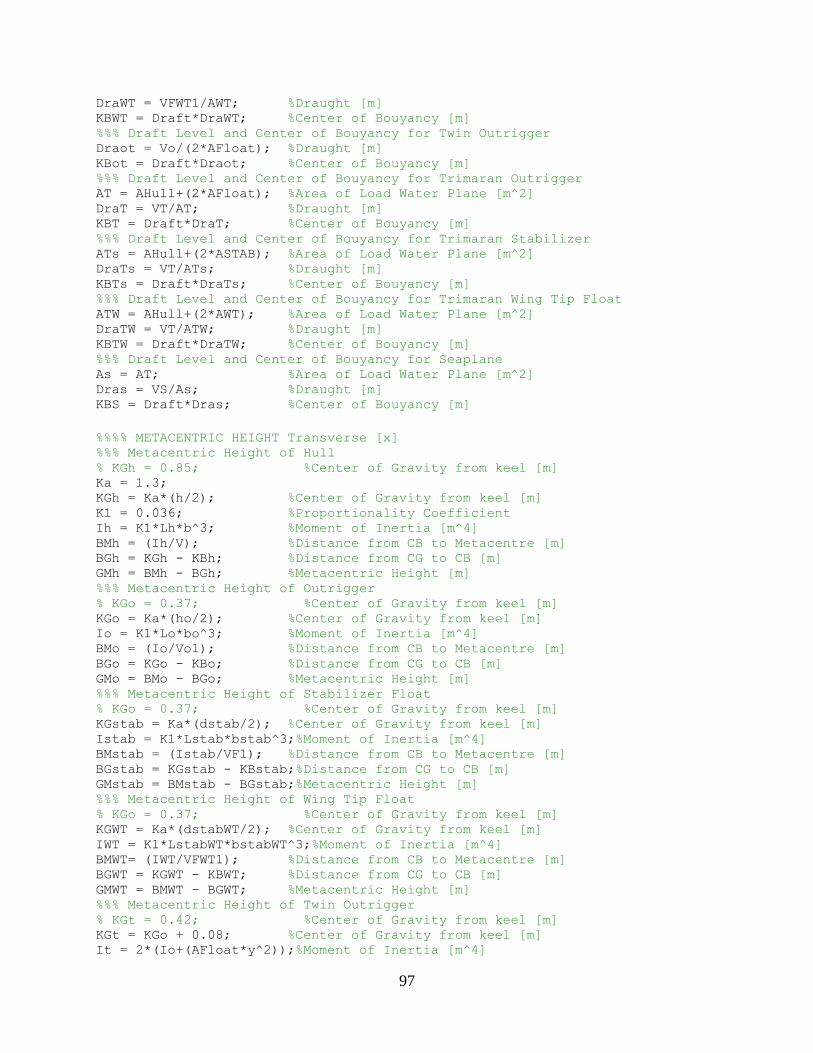
97
DraWT = VFWT1/AWT; %Draught [m] KBWT = Draft*DraWT; %Center of Bouyancy [m] %%% Draft Level and Center of Bouyancy for Twin Outrigger Draot = Vo/(2*AFloat); %Draught [m] KBot = Draft*Draot; %Center of Bouyancy [m] %%% Draft Level and Center of Bouyancy for Trimaran Outrigger AT = AHull+(2*AFloat); %Area of Load Water Plane [m^2] DraT = VT/AT; %Draught [m] KBT = Draft*DraT; %Center of Bouyancy [m] %%% Draft Level and Center of Bouyancy for Trimaran Stabilizer ATs = AHull+(2*ASTAB); %Area of Load Water Plane [m^2] DraTs = VT/ATs; %Draught [m] KBTs = Draft*DraTs; %Center of Bouyancy [m] %%% Draft Level and Center of Bouyancy for Trimaran Wing Tip Float ATW = AHull+(2*AWT); %Area of Load Water Plane [m^2] DraTW = VT/ATW; %Draught [m] KBTW = Draft*DraTW; %Center of Bouyancy [m] %%% Draft Level and Center of Bouyancy for Seaplane As = AT; %Area of Load Water Plane [m^2] Dras = VS/As; %Draught [m] KBS = Draft*Dras; %Center of Bouyancy [m]
%%%% METACENTRIC HEIGHT Transverse [x] %%% Metacentric Height of Hull % KGh = 0.85; %Center of Gravity from keel [m] Ka = 1.3; KGh = Ka*(h/2); %Center of Gravity from keel [m] K1 = 0.036; %Proportionality Coefficient Ih = K1*Lh*b^3; %Moment of Inertia [m^4] BMh = (Ih/V); %Distance from CB to Metacentre [m] BGh = KGh - KBh; %Distance from CG to CB [m] GMh = BMh - BGh; %Metacentric Height [m] %%% Metacentric Height of Outrigger % KGo = 0.37; %Center of Gravity from keel [m] KGo = Ka*(ho/2); %Center of Gravity from keel [m] Io = K1*Lo*bo^3; %Moment of Inertia [m^4] BMo = (Io/Vo1); %Distance from CB to Metacentre [m] BGo = KGo - KBo; %Distance from CG to CB [m] GMo = BMo - BGo; %Metacentric Height [m] %%% Metacentric Height of Stabilizer Float % KGo = 0.37; %Center of Gravity from keel [m] KGstab = Ka*(dstab/2); %Center of Gravity from keel [m] Istab = K1*Lstab*bstab^3;%Moment of Inertia [m^4] BMstab = (Istab/VF1); %Distance from CB to Metacentre [m] BGstab = KGstab - KBstab;%Distance from CG to CB [m] GMstab = BMstab - BGstab;%Metacentric Height [m] %%% Metacentric Height of Wing Tip Float % KGo = 0.37; %Center of Gravity from keel [m] KGWT = Ka*(dstabWT/2); %Center of Gravity from keel [m] IWT = K1*LstabWT*bstabWT^3;%Moment of Inertia [m^4] BMWT= (IWT/VFWT1); %Distance from CB to Metacentre [m] BGWT = KGWT - KBWT; %Distance from CG to CB [m] GMWT = BMWT - BGWT; %Metacentric Height [m] %%% Metacentric Height of Twin Outrigger % KGt = 0.42; %Center of Gravity from keel [m] KGt = KGo + 0.08; %Center of Gravity from keel [m] It = 2*(Io+(AFloat*y^2));%Moment of Inertia [m^4]

98
BMt = (It/Vo); %Distance from CB to Metacentre [m] BGt = KGt - KBot; %Distance from CG to CB [m] GMt = BMt - BGt; %Metacentric Height [m] %%% Metacentric Height of Twin Stabilizer % KGt = 0.42; %Center of Gravity from keel [m] KGts = KGstab + 0.08; %Center of Gravity from keel [m] Its = 2*(Istab+(ASTAB*l^2));%Moment of Inertia [m^4] BMts = (Its/(VF1*2)); %Distance from CB to Metacentre [m] BGts = KGts - KBstab; %Distance from CG to CB [m] GMts = BMts - BGts; %Metacentric Height [m] %%% Metacentric Height of Twin Wing Tip Float % KGt = 0.42; %Center of Gravity from keel [m] KGtW = KGWT + 0.08; %Center of Gravity from keel [m] ItW = 2*(IWT+(AWT*(b2/2)^2));%Moment of Inertia [m^4] BMtW = (ItW/(VFWT1*2)); %Distance from CB to Metacentre [m] BGtW = KGtW - KBWT; %Distance from CG to CB [m] GMtW = BMtW - BGtW; %Metacentric Height [m] %%% Metacentric Height of Trimaran Outrigger % KGT = 0.826; %Center of Gravity from keel [m] KGT = (KGh/2.15) + KGt; %Center of Gravity from keel [m] IT = Ih + It; %Moment of Inertia [m^4] BMT = (IT/VT); %Distance from CB to Metacentre [m] BGT = KGT - KBT; %Distance from CG to CB [m] GMT = BMT - BGT; %Metacentric Height [m] %%% Metacentric Height of Trimaran Stabilizer % KGT = 0.826; %Center of Gravity from keel [m] KGTs = (KGh/2.15) + KGts;%Center of Gravity from keel [m] ITs = Ih + Its; %Moment of Inertia [m^4] BMTs = (ITs/VT); %Distance from CB to Metacentre [m] BGTs = KGTs - KBTs; %Distance from CG to CB [m] GMTs = BMTs - BGTs; %Metacentric Height [m] %%% Metacentric Height of Trimaran Wing Tip Float % KGT = 0.826; %Center of Gravity from keel [m] KGTW = (KGh/2.15) + KGtW;%Center of Gravity from keel [m] ITW = Ih + ItW; %Moment of Inertia [m^4] BMTW = (ITW/VT); %Distance from CB to Metacentre [m] BGTW = KGTW - KBTW; %Distance from CG to CB [m] GMTW = BMTW - BGTW; %Metacentric Height [m] %%% Metacentric Height of Seaplane Trimaran KGS = 1.75; %Center of Gravity from keel [m] % KGS = CGL + (KGT*1.75); %Center of Gravity from keel [m] IS = IT; %Moment of Inertia of Trimaran[m^4] BMS = (IS/VS); %Distance from CB to Metacentre [m] BGS = KGS - KBS; %Distance from CG to CB [m] GMS = BMS - BGS; %Metacentric Height [m] %%% Metacentric Height of Seaplane Stabilizer KGSs = 1.84; %Center of Gravity from keel [m] % KGSs = CGL + (KGTs/3.5);%Center of Gravity from keel [m] ISs = ITs; %Moment of Inertia of Trimaran[m^4] BMSs = (ISs/VS); %Distance from CB to Metacentre [m] BGSs = KGSs - KBTs; %Distance from CG to CB [m] GMSs = BMSs - BGSs; %Metacentric Height [m] %%% Metacentric Height of Seaplane Wing Tip Float KGSW = 1.84; %Center of Gravity from keel [m] % KGSW = CGL + (KGTW/3.5);%Center of Gravity from keel [m] ISW = ITW; %Moment of Inertia of Trimaran[m^4] BMSW = (ISW/VS); %Distance from CB to Metacentre [m]

99
BGSW = KGSW - KBTW; %Distance from CG to CB [m] GMSW = BMSW - BGSW; %Metacentric Height [m]
%%%% METACENTRIC HEIGHT LONGITUDINAL [y] %%% Metacentric Height of Hull Ihy = K1*Lh^3*b; %Moment of Inertia [m^4] BMhy = (Ihy/V); %Distance from CB to Metacentre [m] GMhy = BMhy - BGh; %Metacentric Height [m] %%% Metacentric Height of Outrigger Ioy = K1*Lo^3*bo; %Moment of Inertia [m^4] BMoy = (Ioy/Vo1); %Distance from CB to Metacentre [m] GMoy = BMoy - BGo; %Metacentric Height [m] %%% Metacentric Height of Twin Outrigger Ity = 2*(Ioy+(AFloat*y^2));%Moment of Inertia [m^4] BMty = (Ity/Vo); %Distance from CB to Metacentre [m] GMty = BMty - BGt; %Metacentric Height [m] %%% Metacentric Height of Trimaran ITy = Ihy + Ity; %Moment of Inertia [m^4] BMTy = (ITy/VT); %Distance from CB to Metacentre [m] GMTy = BMTy - BGT; %Metacentric Height [m] %%% Metacentric Height of Seaplane ISy = ITy; %Moment of Inertia of Trimaran[m^4] BMSy = (ISy/VS); %Distance from CB to Metacentre [m] GMSy = BMSy - BGS; %Metacentric Height [m]
%% Air Ministry Minimum Requirements for Stability fprintf(' Air Ministry Minimum Requirements for Stability') disp(' ') %Stability of Hull TGMh = 4*(V)^(1/3); %Transverse Metacentric Height LGMh = 6*(V)^(1/3); %Longitudinal Metacentric Height if GMh >= TGMh fprintf('GMh = Pass'); else fprintf('GMh = Fail'); end disp(' ') if GMhy >= LGMh fprintf('GMhy = Pass'); else fprintf('GMhy = Fail'); end disp(' ') % Stability of Outrigger TGMo = 4*(Vo1)^(1/3); %Transverse Metacentric Height LGMo = 6*(Vo1)^(1/3); %Longitudinal Metacentric Height if GMo >= TGMo fprintf('GMo = Pass'); else fprintf('GMo = Fail'); end disp(' ') if GMoy >= LGMo fprintf('GMoy = Pass'); else fprintf('GMoy = Fail');

100
end disp(' ') %Stability of Twin Floats TGMt = 4*(Vo)^(1/3); %Transverse Metacentric Height LGMt = 6*(Vo)^(1/3); %Longitudinal Metacentric Height if GMt >= TGMt fprintf('GMt = Pass'); else fprintf('GMt = Fail'); end disp(' ') if GMty >= LGMt fprintf('GMty = Pass'); else fprintf('GMty = Fail'); end disp(' ') % Stability of Trimaran TGMT = 4*(VT)^(1/3); %Transverse Metacentric Height LGMT = 6*(VT)^(1/3); %Longitudinal Metacentric Height if GMT >= TGMT fprintf('GMT = Pass'); else fprintf('GMT = Fail'); end disp(' ') if GMTy >= LGMT fprintf('GMTy = Pass'); else fprintf('GMTy = Fail'); end disp(' ') % Stability of Seaplane TGMS = 4*(VS)^(1/3); %Transverse Metacentric Height LGMS = 6*(VS)^(1/3); %Longitudinal Metacentric Height if GMS >= TGMS fprintf('GMS = Pass'); else fprintf('GMS = Fail'); end disp(' ') if GMSy >= LGMS fprintf('GMSy = Pass'); else fprintf('GMSy = Fail'); end
%% Righting Moment theta = 0:90; %%% Float Track location RM = delT*y*cos(theta*(pi/180)); %%% Float Track location RMF = delT*l*cos(theta*(pi/180)); %%% Float Track location RMFWT = delT*(b2/2)*cos(theta*(pi/180)); %%% Righting Moment for Hull RMh = delH*sin(theta*(pi/180))*GMh;

101
%%% Righting Moment for Outrigger RMo = delO1*sin(theta*(pi/180))*GMo; %%% Righting Moment for Stabilizer Float RMstab = delF*sin(theta*(pi/180))*GMstab; %%% Righting Moment for Wing Tip Float RMWT = delFWT*sin(theta*(pi/180))*GMWT; %%% Righting Moment for Seaplane Trimaran RMS = delT*sin(theta*(pi/180))*GMS; %%% Righting Moment for Seaplane Stabilizer RMSs = delT*sin(theta*(pi/180))*GMSs; %%% Righting Moment for Seaplane Wing Tip Float RMSW = delT*sin(theta*(pi/180))*GMSW;
%Maximum Righting Moment and Max angle of tilting thetamax = 90; %Max angle of Tilting [deg] RMSmax = delT*sin(thetamax*(pi/180))*GMS; %Max Rigthing Moment [kg m] phi = RMSmax./(delT*y); phimax = acos(phi)*(180/pi); %Max allowed angle of Tilting
%% Stability in Wind B = y; %Beam between the centerlines of the outer hulls [m] CE = GMSy; %Height of the center of effort above the CG [m] SA = 0:50; %Sail Area [m^2] SF = 9.48*sqrt((0.5*B*GW)./(SA*CE));%Wind Speed [m/s]
%% Plots figure plot(theta,RMS,'k',theta,RMSs,theta,RMSW,'Linewidth',2) xlabel('Angle of Inclination [deg]') ylabel('Righting Moment [Kg m]') title('Righting Moment Transverse Stability') legend('Seaplane Trimaran','Seaplane Stabilizer','Seaplane Wing Tip Float')
%% Results disp(' ') fprintf('-----------------------------------------------------') fprintf('\n Stability Parameters\n') disp(' ') fprintf('\n Centre of Bouyancy, Centre of Gravity and Draft Line\n') fprintf('\n Hull \n') fprintf('\n Draft [m] = %g\n', Drah) fprintf('\n Centre of Bouyancy [m] = %g\n', KBh) fprintf('\n Centre of Gravity [m] = %g\n', KGh) fprintf('\n Metacentre Transverse [m] = %g\n', BMh) fprintf('\n Metacentric Height Transverse [m] = %g\n', GMh) fprintf('\n Metacentre Longitudinal [m] = %g\n', BMhy) fprintf('\n Metacentric Height Longitudinal [m] = %g\n', GMhy) disp(' ') fprintf('\n Outrigger \n') fprintf('\n Draft [m] = %g\n', Drao) fprintf('\n Centre of Bouyancy [m] = %g\n', KBo) fprintf('\n Centre of Gravity [m] = %g\n', KGo) fprintf('\n Metacentre Transverse [m] = %g\n', BMo) fprintf('\n Metacentric Height Transverse [m] = %g\n', GMo) fprintf('\n Metacentre Longitudinal [m] = %g\n', BMoy) fprintf('\n Metacentric Height Longitudinal [m] = %g\n', GMoy)

102
disp(' ') fprintf('\n Stabilizer Float \n') fprintf('\n Draft [m] = %g\n', Drastab) fprintf('\n Centre of Bouyancy [m] = %g\n', KBstab) fprintf('\n Centre of Gravity [m] = %g\n', KGstab) fprintf('\n Metacentre Transverse [m] = %g\n', BMstab) fprintf('\n Metacentric Height Transverse [m] = %g\n', GMstab) disp(' ') fprintf('\n Wing Tip Float \n') fprintf('\n Draft [m] = %g\n', DraWT) fprintf('\n Centre of Bouyancy [m] = %g\n', KBWT) fprintf('\n Centre of Gravity [m] = %g\n', KGWT) fprintf('\n Metacentre Transverse [m] = %g\n', BMWT) fprintf('\n Metacentric Height Transverse [m] = %g\n', GMWT) disp(' ') fprintf('\n Twin Floats \n') fprintf('\n Draft [m] = %g\n', Drao) fprintf('\n Centre of Bouyancy [m] = %g\n', KBo) fprintf('\n Centre of Gravity [m] = %g\n', KGt) fprintf('\n Metacentre Transverse [m] = %g\n', BMt) fprintf('\n Metacentric Height Transverse [m] = %g\n', GMt) fprintf('\n Metacentre Longitudinal [m] = %g\n', BMty) fprintf('\n Metacentric Height Longitudinal [m] = %g\n', GMty) disp(' ') fprintf('\n Trimaran \n') fprintf('\n Draft [m] = %g\n', DraT) fprintf('\n Centre of Bouyancy [m] = %g\n', KBT) fprintf('\n Centre of Gravity [m] = %g\n', KGT) fprintf('\n Metacentre Transverse [m] = %g\n', BMT) fprintf('\n Metacentric Height Transverse [m] = %g\n', GMT) fprintf('\n Metacentre Longitudinal [m] = %g\n', BMTy) fprintf('\n Metacentric Height Longitudinal [m] = %g\n', GMTy) disp(' ') fprintf('\n Seaplane Trimaran\n') fprintf('\n Draft [m] = %g\n', Dras) fprintf('\n Centre of Bouyancy [m] = %g\n', KBS) fprintf('\n Centre of Gravity [m] = %g\n', KGS) fprintf('\n Metacentre Transverse [m] = %g\n', BMS) fprintf('\n Metacentric Height Transverse [m] = %g\n', GMS) fprintf('\n Metacentre Longitudinal [m] = %g\n', BMSy) fprintf('\n Metacentric Height Longitudinal [m] = %g\n', GMSy) disp(' ') fprintf('\n Seaplane Stabilizer\n') fprintf('\n Draft [m] = %g\n', DraTs) fprintf('\n Centre of Bouyancy [m] = %g\n', KBTs) fprintf('\n Centre of Gravity [m] = %g\n', KGSs) fprintf('\n Metacentre Transverse [m] = %g\n', BMSs) fprintf('\n Metacentric Height Transverse [m] = %g\n', GMSs) disp(' ') fprintf('\n Seaplane Wing Tip Float\n') fprintf('\n Draft [m] = %g\n', DraTW) fprintf('\n Centre of Bouyancy [m] = %g\n', KBTW) fprintf('\n Centre of Gravity [m] = %g\n', KGSW) fprintf('\n Metacentre Transverse [m] = %g\n', BMSW) fprintf('\n Metacentric Height Transverse [m] = %g\n', GMSW) fprintf('\n-----------------------------------------------------\n')
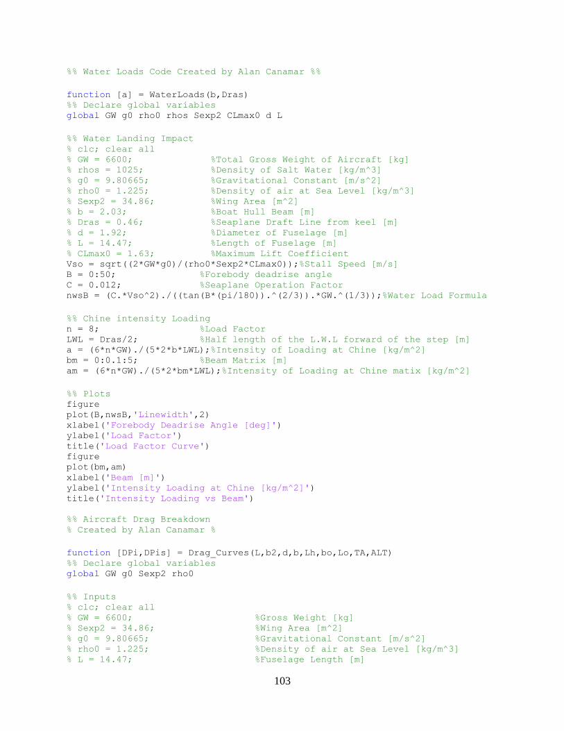
103
%% Water Loads Code Created by Alan Canamar %%
function [a] = WaterLoads(b,Dras) %% Declare global variables global GW g0 rho0 rhos Sexp2 CLmax0 d L
%% Water Landing Impact % clc; clear all % GW = 6600; %Total Gross Weight of Aircraft [kg] % rhos = 1025; %Density of Salt Water [kg/m^3] % g0 = 9.80665; %Gravitational Constant [m/s^2] % rho0 = 1.225; %Density of air at Sea Level [kg/m^3] % Sexp2 = 34.86; %Wing Area [m^2] % b = 2.03; %Boat Hull Beam [m] % Dras = 0.46; %Seaplane Draft Line from keel [m] % d = 1.92; %Diameter of Fuselage [m] % L = 14.47; %Length of Fuselage [m] % CLmax0 = 1.63; %Maximum Lift Coefficient Vso = sqrt((2*GW*g0)/(rho0*Sexp2*CLmax0));%Stall Speed [m/s] B = 0:50; %Forebody deadrise angle C = 0.012; %Seaplane Operation Factor nwsB = (C.*Vso^2)./((tan(B*(pi/180)).^(2/3)).*GW.^(1/3));%Water Load Formula
%% Chine intensity Loading n = 8; %Load Factor LWL = Dras/2; %Half length of the L.W.L forward of the step [m] a = (6*n*GW)./(5*2*b*LWL);%Intensity of Loading at Chine [kg/m^2] bm = 0:0.1:5; %Beam Matrix [m] am = (6*n*GW)./(5*2*bm*LWL);%Intensity of Loading at Chine matix [kg/m^2]
%% Plots figure plot(B,nwsB,'Linewidth',2) xlabel('Forebody Deadrise Angle [deg]') ylabel('Load Factor') title('Load Factor Curve') figure plot(bm,am) xlabel('Beam [m]') ylabel('Intensity Loading at Chine [kg/m^2]') title('Intensity Loading vs Beam')
%% Aircraft Drag Breakdown % Created by Alan Canamar %
function [DPi,DPis] = Drag_Curves(L,b2,d,b,Lh,bo,Lo,TA,ALT) %% Declare global variables global GW g0 Sexp2 rho0
%% Inputs % clc; clear all % GW = 6600; %Gross Weight [kg] % Sexp2 = 34.86; %Wing Area [m^2] % g0 = 9.80665; %Gravitational Constant [m/s^2] % rho0 = 1.225; %Density of air at Sea Level [kg/m^3] % L = 14.47; %Fuselage Length [m]

104
% b2 = 19.08; %Wing Span [m] % d = 1.92; %Fuselage Height [m] % b = 2.03; %Hull beam [m] % Lh = L; %Main Hull Length [m] % bo = 0.59; %Outrigger Beam [m] % Lo = 0.5*Lh; %Outrigger Length [m] % TA = 25500; %Thrust Available [N] % ALT = 4200; %Cruising altitude [m] Vel = 150; %Speed [m/s]
%% Initial Calculations dV = 1; %Speed Change V = 15:dV:Vel; %Speed Matrix h0 = 0; %Altitude at sea level [m] G = 1.4; %Ratio of specific heat of air (gamma) R = 286.9; %Gas constant [J/kg*K] T0 = 287.827; %Temperature at sea level [K] a_L = -0.0065; %Lapse Rate [K/m] T = T0; % T = T0+(a_L*(ALT-h0)); %Temperature altitude gradient [K] rho = rho0; % rho = rho0*(1-((2.2558*10^-5)*ALT))^4.255;%Density altitude gradient
[kg/m^3] a = sqrt(G*R.*T); %Local speed of sound [m/s] M = V./a; %Mach number q = 0.5*rho*V.^2; %Dynamic Pressure [Pa]
%% Calculation of Dynamic Viscosity of air T00 = 291.15; %Reference Temperature [K] v0 = 18.27*10^-6; %Reference Viscosity [Pa-s] C = 120; %Sutherlands Constant [K] v = v0; % v = v0.*((T00+C)./(T+C)).*((T./T00).^(3/2));%Dynamic viscosity [Pa-s]
%% Flat plate drag area of the fuselage %Fuselage Geometry %1 stands for fuselage if L == 0; f1 = 0; else Ln = 3.52; %Length of the Nose of Fuselage [m] Lt = 4.87; %Length of the Tail of Fuselage [m] Lfu = L-Ln-Lt; %Length of Fuselage [m] Swetn = 0.75*pi*d*Ln; %Wetted area of the nose [m^2] Swetf = (0.5*pi*d^2)+(pi*d*Lfu);%Wetted area of fuselage [m^2] Swet1 = Swetn+Swetf; %Wetted Area [m^2] Q = 1; %Interference Factor Re1 = (V*L*rho)/v; %Reynolds Number Cf1 = 0.455./(log10(Re1)).^2.58;%Friction coefficient Amax = (pi*d^2)/4; %Fuselage Cross Area [m^2] ld = L/sqrt((4/pi)*Amax); %Fineness ratio F1 = 1+(60/(ld^3))+(ld/400); %Fuselage Form Factor f1 = Cf1*F1*Q*Swet1; %Flat plate drag area [m^2] end
%% Flat Plate Drag Area of the wing

105
%Wing Geometry %2 stands for wing if b2 == 0; f2 = 0; else cT2 = 1.12; %Wing Tip Chord [m] cr2 = 2.534; %Wing Root Chord [m] zeta2 = 0; %Wing Sweep Angle [degree] tc2 = 0.18; %Wing thickness ratio zeta_rad2 = zeta2*(pi/180); %Sweep Angle [rad] if tc2 < 0.05; Swet2 = 2.003*Sexp2; else Swet2 = Sexp2*(1.977+(0.52*tc2)); %Wetted Wing Area [m^2] end lamda2 = cT2/cr2; %Taper ratio mac2 = (2/3)*cr2*(1+lamda2-(lamda2/(1+lamda2))); %Aerodynamic moment [m] Re2 = (V*rho*mac2)/v; %Reynolds Number Cf2 = 0.455./(log10(Re2)).^2.58; %Friction Coefficient z2 = ((2-M.^2).*cos(zeta_rad2))./sqrt((1-M.^2).*cos(zeta_rad2).^2); F2 = 1+(z2*tc2)+(100*tc2^4); %Wing Form Factor f2 = Cf2.*F2.*Q.*Swet2; %Wing drag area [m^2] end
%% Flat Plate Drag area of the horizontal tail %Tail Geometry %3 stands for tail b3 = 1.799; %Horizontal Tail Span [m] if b3 == 0; f3 = 0; else cT3 = 1.054; %Horizontal Tail Taper Chord [m] cr3 = 1.799; %Horizontal Tail Root Chord [m] zeta3 = 5; %Horizontal Tail Sweep Angle
[degree] tc3 = 0.12; %Horizontal Tail Thickness ratio Sexp3 = 9.56; %Horizontal Tail Area [m^2] zeta_rad3 = zeta3*(pi/180); %Sweep Angle [rad] if tc3 < 0.05; Swet3 = 2.003*Sexp3; else Swet3 = Sexp3*(1.977+(0.52*tc3)); %Wetted Tail Area [m^2] end lamda3 = cT3/cr3; %Taper ratio mac3 = (2/3)*cr3*(1+lamda3-(lamda3/(1+lamda3)));%Aerodynamic moment [m] Re3 = (V*rho*mac3)/v; %Reynolds Number Cf3 = 0.455./(log10(Re3)).^2.58; %Friction Coefficient z3 = ((2-M.^2).*cos(zeta_rad3))./sqrt((1-M.^2).*cos(zeta_rad3).^2); F3 = 1+(z3*tc3)+(100*tc3^4); %Tail Form Factor f3 = Cf3.*F3.*Q.*Swet3; %Tail Drag Area [m^2] end
%% Flat Plate Drag area of the vertical tail %Vetical Tail Geometry %4 stands for Vertical tail b4 = 3.31; %Vertical Tail Span [m]

106
if b4 == 0; f4 =0; else cT4 = 1.47; %Vertical Tail Taper Chord [m] cr4 = 2.94; %Vertical Tail Root Chord [m] zeta4 = 35; %Vertical Tail Sweep Angle [degree] tc4 = 0.12; %Vertical Tail Thickness ratio Sexp4 = 7.298; %Vertical Tail Area [m^2] zeta_rad4 = zeta4*(pi/180); %Sweep Angle [rad] if tc4 < 0.05; Swet4 = 2.003*Sexp4; else Swet4 = Sexp4*(1.977+(0.52*tc4)); %Wetted Tail Area [m^2] end lamda4 = cT4/cr4; %Taper ratio mac4 = (2/3)*cr4*(1+lamda4-(lamda4/(1+lamda4)));%Aerodynamic moment [m] Re4 = (V*rho*mac4)/v; %Reynolds Number Cf4 = 0.455./(log10(Re4)).^2.58; %Friction Coefficient z4 = ((2-M.^2).*cos(zeta_rad4))./sqrt((1-M.^2).*cos(zeta_rad4).^2); F4 = 1+(z4*tc4)+(100*tc4^4); %Tail Form Factor f4 = Cf4.*F4.*Q.*Swet4; %Tail Drag Area [m^2] end
%% Flat Plate Drag Area of Engines %Engine Geometry %5 stands for Engine n5 = 2; %Number of Engines if n5 == 0; f5 = 0; else L5 = 2.8; %Engine Length [m] d5 = 1; %Engine Diameter [m] Sexp5 = (0.5*pi*d5^2)+(pi*d5*L5); %Engine Area [m^2] Q5 = 1.5; %Interference factor g5 = L5/d5; %Effective Fineness ratio Re5 = (V*rho*L5)/v; %Reynolds Number Cf5 = 0.455./(log10(Re5)).^2.58; %Friction Coefficient F5 = 1+(0.35/g5); %Form Factor f5 = Cf5.*F5.*Q5.*Sexp5.*n5; %Engine Drag Area [m^2] end
%% Flat Plate Drag Area of Pylons %Pylon Geometry %6 stands for Pylon n6 = 0; %Number of Pylons if n6 == 0; f6 = 0; else cT6 = 0; %Pylon Taper Chord [m] cr6 = 0; %Pylon Root Chord [m] zeta6 = 0; %Pylon Sweep Angle [degree] tc6 = 0; %Pylon Thickness ratio Sexp6 = 0; %Pylon Area [m^2] zeta_rad6 = zeta6*(pi/180); %Sweep Angle [rad] if tc6 < 0.05; Swet6 = 2.003*Sexp6;

107
else Swet6 = Sexp6*(1.977+(0.52*tc6)); %Wetted Pylon Area [m^2] end lamda6 = cT6/cr6; %Taper Ratio mac6=(2/3)*cr6*(1+lamda6-(lamda6/(1+lamda6))); %Aerodynamic moment [m] Re6 = (V*rho*mac6)/v; %Reynolds Number Cf6 = 0.455./(log10(Re6)).^2.58; %Friction Coefficient z6=((2-M^2)*cos(zeta_rad6))/sqrt((1-M^2)*cos(zeta_rad6)^2); F6=1+(z6*tc6)+(100*tc6^4); %Form Factor f6 = Cf6.*F6.*Q.*Swet6.*n6; %Pylon Drag Area [m^2] end
%% Flat Plate Drag Area of the Propeller %Propeller Geometry Nb = 0; %Number of Blades if Nb == 0; fprop = 0; else cb = 0.85; %Average Blade Chord [m] R = 1.04; %Propeller Radius [m] r = 0.5; %Radius of disk [m] s = 0.6; %Height of disk [m] Adisk = (pi*r*s)+(pi*r^2); %Disk Area [m^2] nu = (Nb*cb)./(pi*R); Pf = 1; if Pf == 1; fprop = 0.1*nu*Adisk; %Flat Area Propeller [m^2] else fprop = 0.8*nu*Adisk; %Flat Area Propeller [m^2] end end
%% Flat plate drag area of the Boat Hull %Boat Hull Geometry %b stands for Boat Hull rb = (b/2); %Radius of Boat Hull [m] KA = 0.7; %Proportionality Coefficient AHull = KA*Lh*b; %Area of Load Water Plane of Hull [m^2] Swetb = 0.5*((pi*rb^2)+AHull+(pi*rb*Lh));%Wetted area of Boat Hull [m^2] Qb = 1.25; %Interference Factor Reb = (V*Lh*rho)/v; %Reynolds Number Cfb = 0.455./(log10(Reb)).^2.58;%Friction coefficient Amaxb = (pi*(rb/2)^2)/4; %Boat Hull Cross Area [m^2] ldb = Lh/sqrt((4/pi)*Amaxb); %Fineness ratio Fb = 1+(60/(ldb^3))+(ldb/400); %Boat Hull Form Factor fb = Cfb.*Fb.*Qb.*Swetb; %Flat plate drag area [m^2]
%% Flat Plate Drag Area of Floats %Float Geometry %f stands for Float nf = 2; %Number of Outriggers if nf == 0; ff = 0; else ro = (bo/2); %Radius [m] AFloat = KA*Lo*bo; %Area of Load Water Plane Float [m^2]

108
Sexpf = (0.5*pi*ro^2)+AFloat+(pi*ro*Lo);%Float Exposed Area [m^2] Qf = 1.5; %Interference factor gf = Lo/bo; %Effective Fineness ratio Ref = (V*rho*Lo)/v; %Reynolds Number Cff = 0.455./(log10(Ref)).^2.58; %Friction Coefficient Ff = 1+(0.35/gf); %Form Factor ff = Cff.*Ff.*Qf.*Sexpf.*nf; %Floats Drag Area [m^2] end
%% Flat Plate Drag Area of the Upsweep %Upsweep Geometry mu = 15; %Upsweep angle [Deg] if mu == 0; %Upsweep angle [Deg] fups = 0; else mu_rad = mu*(pi/180); %Upsweep angle [Rad] fups = 3.83*(mu_rad^2.5)*Amax; %Flat Drag Area Upsweep [m^2] end
%% Miscellanous Flat Plate Drag Area of Landplane [m^2] fsub=f1+f2+f3+f4+f5+f6+fups+fprop; %Subtotal flat plate drag area fmisc=0.05*fsub; %Miscellanous flat plate drag area ftotal_air=fsub+fmisc; %Total Flat plate drag area of Landplane
%% Miscellanous Flat Plate Drag Area of Seaplane [m^2] fsub=f1+f2+f3+f4+f5+f6+fups+fprop+fb+ff;%Subtotal flat plate drag area fmisc=0.05*fsub; %Miscellanous flat plate drag area ftotal_sea=fsub+fmisc; %Total Flat plate drag area of seaplane
%% Parasite Drag Coefficient of Landplane and Seaplane CDP = ftotal_air/Sexp2; CDPs = ftotal_sea/Sexp2;
%% Induced Drag AR = b2^2./Sexp2; %Aspect Ratio if zeta2 == 0; e = (1.78*(1-(0.045*(AR.^0.68))))-0.64; else e = (4.61*(1-(0.045*(AR.^0.68)))*(cos(zeta2).^0.15))-3.1; end K = 1./(pi*AR*e); CL = (GW*g0)./(q*Sexp2); %Coefficient of Lift Cdi = CL.^2.*K; %Induced Drag Coefficient
%% Compressibility Drag Mdiv = (-0.25.*CL)+0.91; mdiff = M-Mdiv; CDC = 0.002.*exp(21.652.*mdiff);
%% Total Drag of Aircraft no Floats or Boat Hull [N] DP = q.*Sexp2.*CDP; %Parasite Drag Lanplane[N] Di = q.*Sexp2.*Cdi; %Induced Drag [N] Dc = q.*Sexp2.*CDC; %Compressibility Drag [N] DPi = DP + Di; %Incrompressible Total Drag [N] Cd = CDP+Cdi; %Total Drag Coefficient

109
%% Total Drag of Seaplane [N] DPs = q.*Sexp2.*CDPs; %Parasite Drag Seaplane[N] DPis = DPs + Di; %Incrompressible Total Drag [N] Cds = CDPs+Cdi; %Total Drag Coefficient
%% Thrust Available Ta0 = TA*exp(-0.0099*V); %Available Thrust [N] teta = T./T0; %Temperature Ratio BPR = 10; %Bypass Ratio TAFAN = TA.*(1+(((G-1)/2)*M.^2)).^(G./(G-1)).*(1-(sqrt(teta*0.25).*M)).*(1-
(0.1*BPR.*M)); TAJET = TA.*(1+(((G-1)/2)*M.^2)).^(G./(G-1)).*(1-(sqrt(teta*0.25).*M)); %% Plots figure plot(V,Di,V,DP,V,DPi,'LineWidth',2) xlabel('Velocity [m/s]') ylabel('Force [N] ') title('Drag Curves') legend('Induce Drag','Parasite Drag','Total Drag') figure plot(V,DPi,V,DPis,'k',V,Ta0,'LineWidth',2) xlabel('Velocity [m/s]') ylabel('Force [N] ') title('Thrust Curves') legend('Thrust Required Landplane','Thrust Required Seaplane',... 'TurboProp Engine')
%% WATER RESISTANCE CODE Created By Alan Canamar
function [FTm,Rw] = Water_Resistance(Lh,Lo,b,h,bo,ho,Lstab,bstab,... dstab,bstabWT,LstabWT,dstabWT,VF1,VFWT1,TA,CLmax0,ALT) %% Declare global variables global GW g0 rho0 rhos Sexp2
%% Water Resistance of Seaplane at Takeoff % Airplane Inputs % clc; clear all % GW = 6600; %Total Gross Weight of Aircraft [kg] % rhos = 1025; %Density of Salt Water [kg/m^3] % g0 = 9.80665; %Gravitational Constant [m/s^2] % rho0 = 1.225; %Density of air at Sea Level [kg/m^3] % Sexp2 = 34.86; %Wing Area [m^2] % Cdsi = 0.0082; %Drag increment due to Seaplane configuration extended % Lh = 14.47; %Length [m] % b = 2.03; %Beam [m] % h = 1.319; %Bow Height [m] % Lo = 7.13; %Length [m] % bo = 0.509; %Beam [m] % ho = 0.46; %Bow Height [m] % Lstab = 3.82; %Length [m] % bstab = 0.95; %Beam [m] % dstab = 0.48; %Bow Height [m] % LstabWT = 2.60; %Length [m] % bstabWT = 0.65; %Beam [m] % dstabWT = 0.32; %Bow Height [m]

110
% CLmax0 = 1.63; %Max Coefficient of Lift % TA = 25000; %Thrust Available [N] % ALT = 4200; %Cruising Altitude [m] % VF1 = 1.7423; % VFWT1 = 0.5479; incCLflap = 0.45; %Increment of CL due to flap configuration Clmax18 = CLmax0;%Max Coefficient of Lift due to Flap v = 1.83*10^-6; %Dynamic Viscosity of Salt Water [m^2/s] VS1 = sqrt((2*GW*g0)./(Clmax18*rho0*Sexp2));%Stall Speed [m/s] Vlof = 1.2*VS1; %Lift off Speed [m/s] V = 0:Vlof; %Takeoff Speed [m/s]
%% Volume Calculations BouyR = 1.9; %Bouyancy Reserve [Percent] HullR = 1.5; %Hull Displacement [Percent] OutR = BouyR - HullR; %Outrigger Displacement [Percent] delT = BouyR*GW; %Trimaran Displacement Weight [kg] delH = HullR*GW; %Hull Displacement Weight [kg] delO = OutR*GW; %Outrigger Displacement Weight [kg] delO1 = delO/2; %One Outrigger Displacement Weight [kg] Vol = delH/rhos; %Hull Displacement Volume [m^3] Vo = delO/rhos; %Twin Outrigger Displacement Volume [m^3] Vo1 = delO1/rhos; %One Outrigger Displacement Volume [m^3] VT = Vol+Vo; %Trimaran Displacement Volume [m^3] VS = delT/rhos; %Seaplane Displacement Volume [m^3]
%% Avialable Thrust Curves h0 = 0; %Altitude at sea level [m] G = 1.4; %Ratio of specific heat of air (gamma) R = 286.9; %Gas constant [J/kg*K] T0 = 287.827; %Temperature at sea level [K] Pasl = 101325; %Atmospheric Pressure at Sea Level [Pa] a_L = -0.0065; %Lapse Rate [K/m] T = T0+(a_L*(ALT-h0)); %Temperature altitude gradient [K] a = sqrt(G*R.*T0); %Local speed of sound [m/s] Mach = V./a; %Mach Number BPR = 10; %Bypass Ratio C = 0.25; %Thrust Constant T_cruise = T0+(a_L*(h0)); %Temperature altitude gradient [K] T_T0 = T_cruise./T0; %Temperature Ratio TATOF = TA*exp(-0.0099*V); %Max Take-off Thrust Curve at 0 Altitude [N] TAFAN = TA.*(1+(((G-1)/2)*Mach.^2)).^(G./(G-1)).*(1-
(sqrt(T_T0*C).*Mach)).*(1-(0.1*BPR.*Mach)); TAJET = TA.*(1+(((G-1)/2)*Mach.^2)).^(G./(G-1)).*(1-(sqrt(T_T0*C).*Mach));
%% Water Resistance of Boat Hull % Inputs KA = 0.7; %Proportionality Coefficient AHull = KA*Lh*b; %Area of Load Water Plane of Hull [m^2] AFloat = KA*Lo*bo; %Area of Load Water Plane Float [m^2] AStab = KA*Lstab*bstab; %Area of Load Water Plane Float [m^2] AWT = KA*LstabWT*bstabWT; %Area of Load Water Plane Float [m^2] Velh = 5.07*sqrt(Lh); %Hull Speed [m/s] Reh = (Velh*Lh)./v; %Reynolds Number for Boat Hull Cfh = 0.075./((log10(Reh)-2).^2); %Friction Coefficient Kh = 19*((Vol./(Lh*b*h))*(b/Lh))^2;%Form Factor

111
CVh = (1+Kh)*Cfh; %Coefficient of Viscous Resistance Fnh = Velh./(sqrt(g0*Lh)); %Froude Number CWh = CVh/0.6; %Wave Coefficient CTh = CVh + CWh; %Coefficient of Friction Resistance Fh = CTh*0.5*rhos*AHull.*Velh.^2; %Frictional Resistance [N]
%% Water Resistance of Floats % Inputs Velo = 5.07*sqrt(Lo); %Hull Speed [m/s] Reo = (Velo*Lo)./v; %Reynolds Number for Boat Hull Cfo = 0.075./((log10(Reo)-2).^2); %Friction Coefficient Ko = 19*((Vo1./(Lo*bo*ho))*(bo/Lo))^2;%Form Factor CVo = (1+Ko)*Cfo; %Coefficient of Viscous Resistance Fno = Velo./(sqrt(g0*Lo)); %Froude Number CWo = CVo/0.6; %Wave Coefficient CTo = CVo + CWo; %Coefficient of Friction Resistance Fo = CTo*0.5*rhos*AFloat.*Velo.^2;%Frictional Resistance [N] Kst = 19*((VF1./(Lstab*bstab*dstab))*(bstab/Lstab))^2;%Form Factor KWT = 19*((VFWT1./(LstabWT*bstabWT*dstabWT))*(bstabWT/LstabWT))^2;%Form
Factor
%% Total Water Resistance of Trimaran [N] VelT = 5.07*sqrt(Lh+(2*Lo)); %Hull Speed [m/s] FnT = VelT./(sqrt(g0*(Lh+(2*Lo))));%Froude Number CTT = CTh + (2*CTo); %Coefficient of Friction Resistance FT = CTT*0.5*rhos*(AHull+(2*AFloat)).*VelT.^2;%Frictional Resistance [N] FT1 = Fh+(2*Fo); %Total Frictional Resistance [N]
%% Water Resistance Curves
%Resistance Calculation for Boat Hull deltaAreaMax = 0.8; %Max Hull Area deltaAreaMin = 0; %Min Hull Area deltaArea = str2double(sprintf('%.4f', deltaAreaMax/length(V))); AHullm = AHull*(deltaAreaMax:-deltaArea:deltaAreaMin);%Matrix Rehm = ((V.*Lh)./v); %Reynolds Number for Boat Hull Cfhm = 0.075./(((log10(Rehm))-2).^2);%Friction Coefficient CVhm = (1+Kh)*Cfhm; %Coefficient of Viscous Resistance CWhm = CVhm/0.6; %Wave Coefficient CThm = CVhm + CWhm; %Coefficient of Friction Resista Fnhm = V./(sqrt(g0*Lh)); %Froude Number Fhm = (CThm*0.5*rhos.*AHullm.*V.^2);%Frictional Resistance [N] %Resistance Calculation for Outriggers AFloatm = AFloat*(deltaAreaMax:-deltaArea:deltaAreaMin);%Matrix Reom = ((V.*Lo)./v); %Reynolds Number for Boat Hull Cfom = 0.075./(((log10(Reom))-2).^2);%Friction Coefficient CVom = (1+Ko)*Cfom; %Coefficient of Viscous Resistance CWom = CVom/0.6; %Wave Coefficient CTom = CVom + CWom; %Coefficient of Friction Resistance Fnom = V./(sqrt(g0*Lo)); %Froude Number Fom = (CTom*0.5*rhos.*AFloatm.*V.^2);%Frictional Resistance [N] %Resistance Calculation for Stabilizers Astabm = AStab*(deltaAreaMax:-deltaArea:deltaAreaMin);%Matrix Restm = ((V.*Lstab)./v); %Reynolds Number for Boat Hull Cfstm = 0.075./(((log10(Restm))-2).^2);%Friction Coefficient CVstm = (1+Kst)*Cfstm; %Coefficient of Viscous Resistance

112
CWstm = CVstm/0.6; %Wave Coefficient CTstm = CVstm + CWstm; %Coefficient of Friction Resistance Fstm = (CTstm*0.5*rhos.*Astabm.*V.^2);%Frictional Resistance [N] %Resistance Calculation Wing Tip Floats AWTm = AWT*(deltaAreaMax:-deltaArea:deltaAreaMin);%Matrix ReWTm = ((V.*LstabWT)./v); %Reynolds Number for Boat Hull CfWTm = 0.075./(((log10(ReWTm))-2).^2);%Friction Coefficient CVWTm = (1+KWT)*CfWTm; %Coefficient of Viscous Resistance CWWTm = CVWTm/0.6; %Wave Coefficient CTWTm = CVWTm + CWWTm; %Coefficient of Friction Resistance FWTm = (CTWTm*0.5*rhos.*AWTm.*V.^2);%Frictional Resistance [N] %Total Water Resistance FTm = (Fhm+(2.*Fom)); %Total Frictional Resistance [N] FTstm = (Fhm+(2.*Fstm)); %Total Frictional Resistance [N] FTWTm = (Fhm+(2.*FWTm)); %Total Frictional Resistance [N] FnTm = Fnhm + (2*Fnom); %Froude Number % %Boat Hull Q = 0.80; %Hull Shape Constant Rw = Q*GW*((V./Vlof) - (V.^2./Vlof.^2));%Water Resistance [N]
%% Plots figure plot(V,FTm,V,TATOF,V,TAJET,V,TAFAN,'Linewidth',2) xlabel('Velocity [m/s]') ylabel('Resistance [N] ') title('Resistance Curves') legend('Water Resistance','Thrust Available Turboprop',... 'Thrust Available JET','Thrust Available Turbofan')
%% Results fprintf('-----------------------------------------------------') fprintf('\n Water Resistance\n') disp(' ') fprintf('\n Boat Hull\n') fprintf('\n Speed Hull [m/s]= %g\n', Velh) fprintf('\n Reynolds Number = %g\n', Reh) fprintf('\n Friction Coefficient = %g\n', Cfh) fprintf('\n Form Factor = %g\n', Kh) fprintf('\n Coefficient of Viscous Resistance = %g\n', CVh) fprintf('\n Froude Number = %g\n', Fnh) fprintf('\n Wave Resistance Coefficient = %g\n', CWh) fprintf('\n Total Water Resistance Coefficient = %g\n', CTh) fprintf('\n Water Frictional Resistance [N] = %g\n', Fh) disp(' ') fprintf('\n Outrigger\n') fprintf('\n Speed Hull [m/s]= %g\n', Velo) fprintf('\n Reynolds Number = %g\n', Reo) fprintf('\n Friction Coefficient = %g\n', Cfo) fprintf('\n Form Factor = %g\n', Ko) fprintf('\n Coefficient of Viscous Resistance = %g\n', CVo) fprintf('\n Froude Number = %g\n', Fno) fprintf('\n Wave Resistance Coefficient = %g\n', CWo) fprintf('\n Total Water Resistance Coefficient = %g\n', CTo) fprintf('\n Water Frictional Resistance [N] = %g\n', Fo) disp(' ') fprintf('\n Trimaran\n')

113
fprintf('\n Speed Hull [m/s]= %g\n', VelT) fprintf('\n Froude Number = %g\n', FnT) fprintf('\n Total Water Resistance Coefficient = %g\n', CTT) fprintf('\n Water Frictional Resistance [N] = %g\n', FT1) fprintf('\n-----------------------------------------------------\n') %% Flight Performance Code % Created by Alan Canamar %
function [Ttotal,Ltotal,Ttotalse,Ltotalse,Vmax,Vmaxs] = Flight_Performance... (EW,EWc,MF,Wpay,Cd,Cdsi,Cdsie,Lh,Lo,b,bo,TA,ALT,Vel) %% Declare global variables global GW g0 rho0 Sexp2 CLmax0
%% General Inputs % clc; clear all % GW = 6600; %Total Gross Weight of Aircraft [kg] % EW = 3900; %Empty Weight of Aircraft [kg] % EWc = 4220; %Empty Weight of Seaplane [kg] % MF = 1300; %Maximum Fuel Weight [kg] % Wpay = 1710; %Maximum Payload Weight [kg] % g0 = 9.80665; %Gravitational Constant [m/s^2] % rho0 = 1.225; %Density of air at Sea Level [kg/m^3] % Sexp2 = 34.86; %Wing Area [m^2] % CLmax0 = 1.63; %Maximum Lift Coefficient % Cd = 0.038; %Coefficient of Drag of Landplane % Cdsi = 0.0074; %Drag increment due to Seaplane configuration extended % Cdsie = 0.0058; %Drag increment due to Seaplane configuration retracted % Lh = 14.47; %Length of Hull [m] % Lo = Lh*0.5; %Length [m] % b = 2.03; %Hull beam [m] % bo = 0.509; %Outrigger Beam [m] % TA = 30500; %Thrust Available [N] % ALT = 4200; %Cruising Altitude [m] % Vel = 470; %Maximum Landplane Speed at cruising altitude [km/hr] GWL = GW*0.97; %Total Gross Weight of Aircraft at Landing [kg]
%% Maximum Speed % Inputs h0 = 0; %Altitude at sea level [m] G = 1.4; %Ratio of specific heat of air (gamma) R = 286.9; %Gas constant [J/kg*K] T0 = 287.827; %Temperature at sea level [K] a_L = -0.0065; %Lapse Rate [K/m]
%Aircraft Turbo Prop Speeds % Maximum Airspeeds of Landplane Vmaxj = Vel*(1000/3600); %Maximum Speed [m/s] if Vmaxj <= 120 Vmax = Vmaxj; else Vmax = Vmaxj.*0.71; %Max Jet Speed [m/s] end
% Maximum Airspeeds of Seaplane Retracted Vmaxs = sqrt((Cd*Vmax^2)./(Cd+Cdsie));

114
%% Takeoff Segment [ttoff,ltoff] = Take_off(GW,g0,rho0,Sexp2,CLmax0,Cd,TA); [ttoffse,ltoffse] = Take_offs(GW,g0,rho0,Sexp2,CLmax0,Cd,TA,Cdsi);
%% Climb Segment for TURBOPROP [tclimb,tclimbse,lclimb,lclimbse,VEAS,VEASs] = Climb(GW,g0,rho0,Sexp2,... CLmax0,Cdsie,Vmax,Vmaxs,ALT,TA);
%% Descent Segment [tdes,ldes,tdese,ldese] = Descent(GWL,g0,rho0,Sexp2,Cd,ALT,Cdsie,... Vmax,Vmaxs);
%% Landing Segment [tland,lland] = Landing(GWL,g0,rho0,Sexp2,CLmax0,Cd); [tlandse,llandse] = Landingse(GWL,g0,rho0,Sexp2,CLmax0,Cd,Cdsi,Cdsie,... Lh,Lo,b,bo);
%% Cruise Segment % Inputs % Landplane VS0 = sqrt((2*GW*g0)/(rho0*Sexp2*CLmax0));%Stall Speed [m/s] T_cruise = T0+(a_L*(ALT-h0));%Temperature altitude gradient [K] T_T0 = T_cruise./T0; %Temperature Ratio Vper = 0.90; %Speed Percentage Vcruise = Vper*Vmax; %Cruise Speed [m/s] a_toff = sqrt(G*R.*T0); %Local speed of sound at takeoff [m/s] a_conti = sqrt(G*R.*T_cruise);%Local speed of sound at takeoff [m/s] Mach_toff = VEAS./a_toff;%Mach Number at Takeoff Mach_max = Vmax./a_conti;%Mach Number at Cruise Mach_idle = VS0./a_toff;%Mach Number at Cruise
%Thrust Specific Fuel [kg/hr/N] ftoff = 0.91; %Throttle Setting at Takeoff fconti = 0.79; %Throttle Setting at Cruise fidle = 0.13; %Throttle Setting at Idle TSFC_toff = ftoff*(0.34+0.19*Mach_toff).*sqrt(T_T0); TSFC_conti = fconti*(0.34+0.19*Mach_max).*sqrt(T_T0); TSFC_idle = fidle*(0.34+0.19*Mach_idle).*sqrt(T_T0); %Thrust Available [N] TA_toff = TA*exp(-0.0099*VEAS); TA_conti = TA*exp(-0.0099*Vmax);
%%% Fuel Calculations %Fuel Consumtion [kg/hr] FCtoff = TA_toff.*TSFC_toff; FCconti = TA_conti*TSFC_conti; FCidle = TA_conti*TSFC_idle;
%%% Fuel Mass calculation [kg] % Landplane mtoff = FCtoff*(ttoff/60); %Takeoff Weight Fuel [kg] mclimb = FCidle*(tclimb/60); %Climb Weight Fuel [kg] mdes = FCidle*(tdes/60); %Descent Weight Fuel [kg] mland = FCidle*(tland/60); %Landing Weight Fuel [kg]

115
%%% Seaplane % Inputs Vcruises = Vper*Vmaxs; %Cruise Speed [m/s] Mach_toffs = VEASs./a_toff;%Mach Number at Takeoff Mach_maxs = Vmaxs./a_conti;%Mach Number at Cruise
%Thrust Specific Fuel [kg/hr/N] TSFC_toffs = ftoff*(0.34+0.19*Mach_toffs).*sqrt(T_T0); TSFC_contis = fconti*(0.34+0.19*Mach_maxs).*sqrt(T_T0); TSFC_idles = fidle*(0.34+0.19*Mach_idle).*sqrt(T_T0); %Thrust Available [N] TA_toffs = TA*exp(-0.0099*VEASs); TA_contis = TA*exp(-0.0099*Vmaxs);
%%% Fuel Calculations %Fuel Consumtion [kg/hr] FCtoffs = TA_toffs.*TSFC_toffs; FCcontis = TA_contis*TSFC_contis; FCidles = TA_contis*TSFC_idles; %Calculations for Seaplane [Rec] mtoffse = FCtoffs*(ttoffse/60);%Takeoff Weight Fuel [kg] mclimbse = FCidles*(tclimbse/60);%Climb Weight Fuel [kg] mdesse = FCidles*(tdese/60); %Descent Weight Fuel [kg] mlandse = FCidles*(tlandse/60);%Landing Weight Fuel [kg]
%% Fuel Mass Calculation of Cruise, Descent and Landing [kg] % Landplane V = (Vcruise*3600)./1000; %Speed [km/hr] msubtotal = mtoff+mclimb+mland+mdes;%Subtotal Weight [kg] mcruise = MF - msubtotal; %Reserve Fuel Weight Fuel [kg] E = mcruise./FCidle; %Endurance [hr] R = E*V; %Range Distance [km]
% Seaplane [Rect] Vs = (Vcruises*3600)./1000; %Speed [km/hr] msubtotalse = mclimbse+mdesse+mtoffse+mlandse;%Subtotal Weight [kg] mcruisese = MF - msubtotalse; %Reserve Fuel Weight Fuel [kg] Ese = mcruisese./FCidles; %Endurance [hr] Rse = Ese*Vs; %Range Distance [km]
%Total time [hr] and distance [km] % Landplane tsubmin = (ttoff+tclimb+tland+tdes)/60; %Subtotal [hr] ttotal = E+tsubmin; %Total Time [hr] ltotal = ltoff+lclimb+ldes+lland+R; %Total Distance [km]
% Seaplane [Rect] tsubminse = (ttoffse+tclimbse+tlandse+tdese)/60;%Subtotal [hr] ttotalse = Ese+tsubminse; %Total Time [hr] ltotalse = ltoff+lclimbse+ldese+lland+Rse;%Total Distance [km]
%% Payload Range Diagram %Calculations for Aircraft mf = GW - EW - Wpay; %Fuel Weight w/Max Payload [kg]

116
Wpaymax = GW - EW - MF; %Payload Weight w/Max Fuel [kg] Wcruise = mf - (msubtotal); %Cruise Fuel Weight w/Max Pay T = Wcruise/FCidle; %Total Cruise Time [hr] L = V*T; %Cruise Distance [km] Ttotal = T+tsubmin; %Total Time [hr] Ltotal = ltoff+lclimb+ldes+lland+L; %Total Distance [km]
%Calculations for Seaplane [Rect] mfs = GW - EWc - Wpay; %Fuel Weight w/Max Payload [kg] Wpaymaxs = GW - EWc - MF; %Payload Weight w/Max Fuel [kg] Wcruisese = mfs - (msubtotalse); %Cruise Fuel Weight [kg] Tse = Wcruisese/FCidles; %Total Cruise Time [hr] Lse = Vs*Tse; %Cruise Distance [km] Ttotalse = Tse+tsubminse; %Total Time [hr] Ltotalse = ltoffse+lclimbse+ldese+llandse+Lse;%Total Distance [km]
%% Plots figure pay = [Wpay Wpay Wpaymax 0]; rangem = [0 Ltotal ltotal (ltotal+(ltotal*0.05))]; payse = [Wpay Wpay Wpaymaxs 0]; rangemse = [0 Ltotalse ltotalse (ltotalse+(ltotalse*0.05))]; plot(rangem,pay,'b',rangemse,payse,'k','Linewidth',2) legend('Landplane','Seaplane') xlabel('Range [km]') ylabel('Payload [kg]') title('Payload Range Diagram')
%% Results fprintf('-----------------------------------------------------') fprintf('\n Range, Time and Fuel Mass Fly Breakdown\n') disp(' ') fprintf('\n Endurance | Landplane |Seaplane|\n') fprintf('\n Takeoff [min]| %g | %g |\n', ttoff,ttoffse) fprintf('\n Climb [min]| %g | %g |\n', tclimb,tclimbse) fprintf('\n Cruising [hr]| %g | %g |\n', E,Ese) fprintf('\n Descent [min]| %g | %g |\n', tdes,tdese) fprintf('\n Landing [min]| %g | %g |\n', tland,tlandse) fprintf('\n Total [hr]| %g | %g |\n', ttotal,ttotalse) disp(' ') fprintf('\n Range [km] | Landplane |Seaplane|\n') fprintf('\n Takeoff | %g | %g |\n', ltoff,ltoffse) fprintf('\n Climb | %g | %g |\n', lclimb,lclimbse) fprintf('\n Cruising | %g | %g |\n', R,Rse) fprintf('\n Descent | %g | %g |\n', ldes,ldese) fprintf('\n Landing | %g | %g |\n', lland,llandse) fprintf('\n Total | %g | %g |\n', ltotal,ltotalse) disp(' ') fprintf('\n Fuel Weight [kg]| Landplane |Seaplane|\n') fprintf('\n Takeoff | %g | %g |\n', mtoff,mtoffse) fprintf('\n Climb | %g | %g |\n', mclimb,mclimbse) fprintf('\n Cruising | %g | %g |\n', mcruise,mcruisese) fprintf('\n Descent | %g | %g |\n', mdes,mdesse) fprintf('\n Landing | %g | %g |\n', mland,mlandse) fprintf('\n Total | %g | %g |\n', MF,MF) fprintf('\n-----------------------------------------------------\n')