Embed Size (px)
Citation preview
Canard-Wing Interference Effects on the Flight
Characteristics of a Transonic Passenger Aircraft
Sean Harrison∗, Ryan Darragh†, Peter E. Hamlington ‡
Turbulence and Energy Systems Laboratory, Department of Mechanical Engineering
University of Colorado, Boulder, Colorado 80309, United States
Mehdi Ghoreyshi§ and Andrew J. Lofthouse¶
High Performance Computing Research Center, U.S. Air Force Academy
USAF Academy, Colorado 80840, United States
Effects of canard–wing interference on the flight characteristics of a civilian transoniccruiser are examined. The aircraft is an unconventional design concept with no historicaldata. The flight characteristics of the aircraft are predicted using aerodynamic models inthe form of look-up tables, generated using high-fidelity computational fluid dynamics sim-ulations and a potential flow solver. These tables contain longitudinal and lateral force andmoment coefficients for different combinations of angle of attack, side-slip angle, and con-trol surface deflections. Dynamic damping derivatives are calculated from time-accuratesimulations of the aircraft models oscillating in pitch, roll, and yaw direction and usinga linear regression estimation method. The static simulations are performed at a Machnumber of 0.117, as reported in wind tunnel experiments, and for two different canardpositions using an overset grid approach. The aerodynamic tables include canard deflec-tions of [-30◦, -10◦, 0, 10◦] at angles of attack ranging from -4◦ to 30◦. Lateral coefficientsare simulated at sideslip angles of -6◦ and 6◦ as well. The dynamic simulations are per-formed for aircraft oscillations about mean angles of attack of zero to ten degrees with amotion frequency of 1Hz and amplitude of 0.5 degrees. The predicted aerodynamic dataare then compared with those measured in wind tunnel experiments and calculated fromthe potential flow solver. The results show that both static and dynamic predictions fromhigh-fidelity flow solver match reasonably well with experiments over the range of anglesconsidered. The comparison plots show that the potential flow solver cannot predict thevortical flows formed over the wing and canard surfaces and thus the breaks seen in theexperimental pitching moments. In addition, the predicted dynamic damping derivativesfrom the potential solver do not match the experimental data due to not having the fuse-lage section in the model and again inability of the solver to predict vortical flows over thevehicle. The aerodynamic models are then used in a stability and control analysis codeto investigate the trim setting and handling quality of two canard designs. Overall, com-puted aerodynamics from the high-fidelity solver leads to similar flight dynamics results asobtained from experimental data. The results show that positioning the canard surface ofthis vehicle closer to the wing requires less canard deflection and thrust force to trim theaircraft. These results confirm that computational fluid dynamics is a promising tool indesign and flight dynamics investigation of aircraft with no historical data.
∗Undergraduate Student, Mechanical Engineering, [email protected]†Graduate Student, Aerospace Engineering Sciences, [email protected]‡Assistant Professor, Mechanical Engineering, [email protected], AIAA Member§Senior Aerospace Engineer, [email protected], AIAA Senior Member¶Director, High Performance Computing Research Center, [email protected], AIAA Senior Member
Distribution A. Approved for Public Release. Distribution unlimited.
1 of 27
American Institute of Aeronautics and Astronautics
Dow
nloa
ded
by U
NIV
ER
SIT
Y O
F C
OL
OR
AD
O B
OU
LD
ER
on
July
7, 2
016
| http
://ar
c.ai
aa.o
rg |
DO
I: 1
0.25
14/6
.201
6-41
79
34th AIAA Applied Aerodynamics Conference
13-17 June 2016, Washington, D.C.
AIAA 2016-4179
This material is declared a work of the U.S. Government and is not subject to copyright protection in the United States.
AIAA Aviation
Nomenclature
a speed of sound, m/sb wing span, mc mean aerodynamic chord, mf frequency, HzCD drag coefficient, D/q∞SCL lift coefficient, L/q∞SCl rolling moment coefficient, Mx/q∞SbCN normal-force coefficient, N/q∞SCn yawing moment coefficient, Mz/q∞SbCm pitching moment coefficient, My/q∞ScCp pressure coefficient (p− p∞)/q∞CY side-force coefficient Y/q∞SD drag force, NDv fuselage vertical diameter, mL lift force, NLf fuselage length, NM Mach number, V/aPDF pitch damping force, 1/radPDM pitch damping moment, 1/radMx,My,Mz rolling, pitching, and yawing moments, N.mp, q, r roll, pitch, and yaw rates, rad/sq∞ dynamic pressure, PaRDM roll damping moment, 1/radSw wing area, m2
Sc canard area, m2
V speed of aircraft, m/sx, y, z grid coordinates, mxc canard apex position, mY DM yaw damping moment, 1/rad
Greek
α angle of attack, deg or radβ side-slip angle, deg or radα time-rate of change of angle of attack, rad/sφc canard deflection angle, degρ air density, kg/m3
µ air viscosity, kg/(m.s)ω angular velocity, rad/sωnd un-damped angular velocity, rad/sθ pitch angle, deg or radζd damping ratio
I. Introduction
Aircraft design is traditionally an expensive process that requires slow, costly, and potentially dangerousflight testing. Traditionally, aircraft conceptual design relies on aerodynamic models generated from pre-vious experience and/or semi-empirical methods.1,2 These estimations are often used to find the stabilityand performance data and to size the control surfaces3 and very likely leading to errors in performancepredictions especially for unconventional configurations. To remedy any detected problem(s) in prototypetesting, sometimes the whole design cycle needs to be repeated. This will significantly increase the aircraftproduction costs.
2 of 27
American Institute of Aeronautics and Astronautics
Dow
nloa
ded
by U
NIV
ER
SIT
Y O
F C
OL
OR
AD
O B
OU
LD
ER
on
July
7, 2
016
| http
://ar
c.ai
aa.o
rg |
DO
I: 1
0.25
14/6
.201
6-41
79
Computational fluid dynamics (CFD) provides a means by which to reduce these costs and provideenough accurate aerodynamic data to use in the design process. With recent advances in automated solidmodeling and grid generation, it is now possible to rapidly create a parameterized watertight surface modelof a concept aircraft. This modeling approach allows designers to screen different configurations prior tobuilding the first prototype. This translates into an overall cost reduction and limiting risks. Specifically,the positioning of lift-producing surfaces such as canards can be manipulated to determine the effects ofmany different configurations on the flight characteristics of an aircraft. The effects of these lifting surfacescan easily be modeled in CFD for various deflection angles, positions, and sizes. These changes can allbe implemented and analyzed computationally, thereby avoiding the need to build and test many differentexperimental models.
In the present study, the effects of different canard configurations on the flight characteristics of a transonicpassenger aircraft concept is examined. This design concept, named the TransCRuiser (TCR), was proposedby the Swedish aerospace company SAAB and was studied using in-house design procedures at SAAB. Theconcept design has undergone several design changes in particular within a European project named SimSAC(Simulating Aircraft Stability and Control)4 and the latest design has an all movable canard surface. Theaddition of a canard provides a secondary lifting surface that could make the aircraft stall-proof, since thecanard will stall before the main wing. This induces a pitching moment on the aircraft, thus reducing itsangle of attack until the canard begins to generate lift again.5 However, the canard tends to reduce thestability of the aircraft when compared to conventional designs.
There is no historical data available to accurately predict the TCR aerodynamic data. The semi-empiricalmethods such as Digital DATCOM6 are limited to model the TCR with a canard at transonic speeds aswell. Ghoreyshi et al.5 detailed some flow features of TCR at different angles of attack and at low subsonicspeeds. Both the leading-edge extension (LEX), wing, and canard have rounded leading edges and are sweptback at and more than 50◦ that causes a complex vortex formation over these surfaces at moderate to highangles of attack. At about α = 12◦, a canard vortex and an inboard (LEX) and outboard wing vortexare present. The wing in the presence of the canard shows smaller inboard vortices than the canardlessconfiguration; this is due to canard downwash effects that reduce the local angle of attack behind the canardspan. On the other hand, the wing outboard vortex is slightly bigger in the presence of the canard. Thecanard vortex becomes larger with increasing angle of attack. At about α = 18◦, the wing vortices merge.At about α = 20◦, the inboard and outboard vortices interact and merge. At α = 24◦ angle of attack,the canard vortex lifts up from the surface as well. At higher angles, the canard in the TCR aircraft hasfavorable effects on the wing aerodynamic performance. The wing behind the canard has a stronger mergedvortex than the wing-only configuration which can delay the vortex breakdown. Note that these complexflow-fields cannot be predicted by a potential flow solver or a vortex lattice method.
Canard placement and surface area on the TCR has been investigated in Ref. 7, in which the primaryconcern was the flight dynamic investigation of the aircraft, as well as by Eliasson et al.,1 whose concernsincluded the selection of the canard position. This study found that by positioning a canard closer to thenose of the aircraft, a smaller deflection was required to achieve trim because the canard has a bigger momentarm about the center of gravity. However, the aerodynamic data in Ref. 1 were generated from a vortexlattice method (VLM) solver and the authors did not state whether the changes in aircraft’s center of gravitywith canard position have been taken into account as well.
Specifically, this paper investigates the effects of two different canard positions on flight characteristicsof the TCR using high-fidelity computational methods. The first position examined is the recommendedposition by Eliasson et al.1 In the second position, canard is placed closer to the wing. Four differentcanard deflection angles are considered: [-30◦, -10◦, 0, 10◦]. The flight dynamics of both configurationswere studied in the Computerized Environment for Aircraft Synthesis and Integrated Optimization Methods(CEASIOM) code.4 The code has aerodynamic, structure, propulsion, weight and balance, and stabilityand control modules. The aerodynamic models are in form of look-up tables. The aerodynamic sourcesavailable in the code are Digital DATCOM and a potential flow solver, named Tornado. The aerodynamictables from external flow solvers and wind tunnel experiments can be input to the code as well. In thiswork, the aerodynamic tables of TCR designs are generated by Cobalt flow solver, Tornado code, and windtunnel experiments. These tables are then used in the SDSA (stability and control module in CEASIOM)to investigate the flight characteristics of TCR aircraft.
There are two main objectives in the present study: 1) to compare the aircraft flight characteristicspredicted from different aerodynamic sources, 2) and to investigate the effects of canard placements on the
3 of 27
American Institute of Aeronautics and Astronautics
Dow
nloa
ded
by U
NIV
ER
SIT
Y O
F C
OL
OR
AD
O B
OU
LD
ER
on
July
7, 2
016
| http
://ar
c.ai
aa.o
rg |
DO
I: 1
0.25
14/6
.201
6-41
79
aircraft handling quality and trim settings. The paper is organized as follows. The next section reviewsthe computational methods. Next, the TCR geometry and grid details are provided. The results are thenpresented and discussed, followed by concluding remarks.
II. Formulation
A. CEASIOM Aircraft Design Code
The CEASIOM code, used in this work, incorporates a parameterized description of the aircraft geometry.The geometry parameters include lifting surfaces, engines, control surfaces, and a fuselage. The liftingsurfaces are defined using the apex position and placement, leading edge sweep angle, dihedral angle, span,wing area, taper ratio. The vertical tail can have a lateral displacement with a tilt angle as well. The strakeis defined by span and leading edge sweep angle. A number of aircraft can be defined using this definition.
CEASIOM starts from these initial parameters and allows the design to be refined by adding wingletand cranked wings. In general, an aircraft geometry can be defined in CEASIOM with approximately 100design variables. The code could generate a water-tight solid model of the design concept as well. Note thatdue to limitation of geometry parameters, the CEASIOM-generated models might have rough geometriesat joints and junctions. However, Ghoreyshi et al.5 showed that these rough geometries do not affect theoverall design trends obtained from viscous flow solvers.
B. Aerodynamic Tables
Aerodynamic models considered in this work are in the form of look-up tables. These tables are thenused in an aircraft stability and control analysis code. The aerodynamic coefficients of TCR can be foundas:
Ci = Ci0(α,M, β) + Ciq(α,M, q).cq
2V+ Cip(α,M, p).
bp
2V+ Cir(α,M, r).
br
2V+ Ciφj (α,M, φj).φj (1)
where i = L,D,m, Y, l, n, representing lift, drag, pitching moment, side-force, rolling and yawing momentcoefficients, respectively. φj = [φc, φa, φr] includes canard, aileron, and rudder deflections, p, q, r are roll,pitch, and yaw rates. Ciq, Cip, Cir are damping derivatives as well. The coefficients in front of the aircraftstates and control are stability derivative which in general are functions of angle of attack, Mach number,and etc. These functions are represented in form of a look-up table as shown in Table 1.
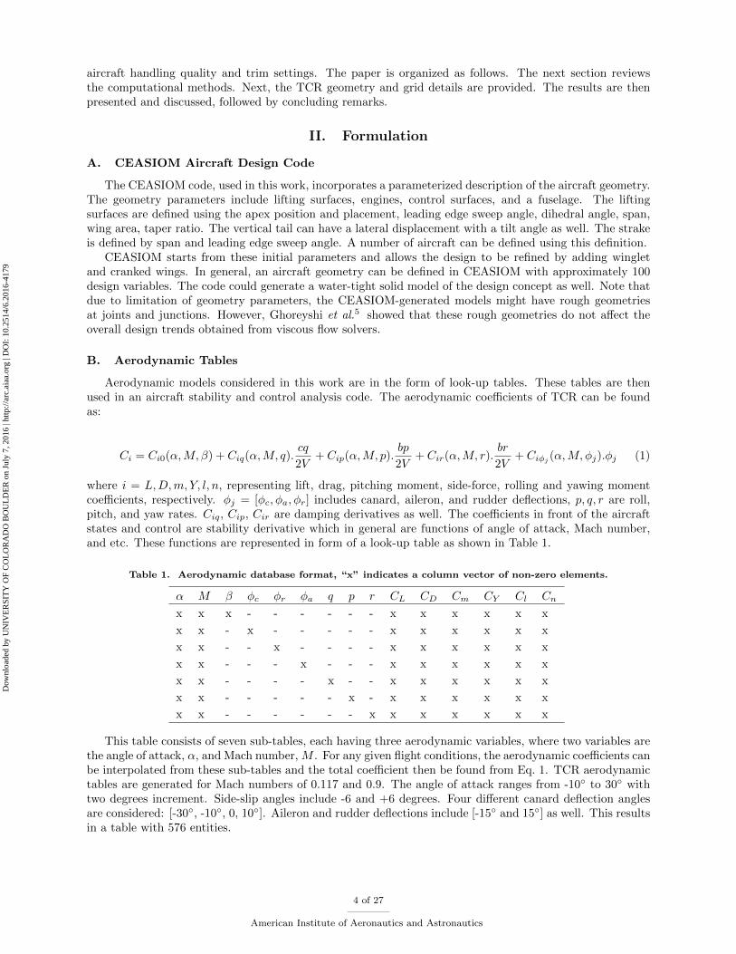
Table 1. Aerodynamic database format, “x” indicates a column vector of non-zero elements.
α M β φc φr φa q p r CL CD Cm CY Cl Cn
x x x - - - - - - x x x x x x
x x - x - - - - - x x x x x x
x x - - x - - - - x x x x x x
x x - - - x - - - x x x x x x
x x - - - - x - - x x x x x x
x x - - - - - x - x x x x x x
x x - - - - - - x x x x x x x
This table consists of seven sub-tables, each having three aerodynamic variables, where two variables arethe angle of attack, α, and Mach number, M . For any given flight conditions, the aerodynamic coefficients canbe interpolated from these sub-tables and the total coefficient then be found from Eq. 1. TCR aerodynamictables are generated for Mach numbers of 0.117 and 0.9. The angle of attack ranges from -10◦ to 30◦ withtwo degrees increment. Side-slip angles include -6 and +6 degrees. Four different canard deflection anglesare considered: [-30◦, -10◦, 0, 10◦]. Aileron and rudder deflections include [-15◦ and 15◦] as well. This resultsin a table with 576 entities.
4 of 27
American Institute of Aeronautics and Astronautics
Dow
nloa
ded
by U
NIV
ER
SIT
Y O
F C
OL
OR
AD
O B
OU
LD
ER
on
July
7, 2
016
| http
://ar
c.ai
aa.o
rg |
DO
I: 1
0.25
14/6
.201
6-41
79
C. Tornado Code
The vortex lattice solver, Tornado,8 can predict a wide range of aircraft stability and control aerodynamicderivatives using a vortex lattice approach. The code models various lifting surfaces such as wing, fin, andcanard. The fuselage is modeled by a thin plate. For control surface deflections, the vortex points locatedat the trailing edge of the flap are rotated around the hinge line which makes the wake change directionslightly.8 The version of the code used in this study does not model the fuselage and include some viscouscorrections.
D. Cobalt Solver
Cobalt solves the unsteady, three-dimensional, compressible Navier-Stokes equations in an inertial ref-erence frame. Arbitrary cell types in two or three dimensions may be used; a single grid therefore can becomposed of different cell types.9 In Cobalt, the Navier-Stokes equations are discretized on arbitrary gridtopologies using a cell-centered finite volume method. Second-order accuracy in space is achieved using theexact Riemann solver of Gottlieb and Groth,10 and least squares gradient calculations using QR factoriza-tion. To accelerate the solution of the discretized system, a point-implicit method using analytic first-orderinviscid and viscous Jacobians is used. A Newtonian sub-iteration method is used to improve the time ac-curacy of the point-implicit method. Tomaro et al.11 converted the code from explicit to implicit, enablingCourant-Friedrichs-Lewy (CFL) numbers as high as 106. In Cobalt, the computational grid can be dividedinto group of cells, or zones, for parallel processing, where high performance and scalability can be achievedeven on ten thousands of processors. Some available turbulence models in Cobalt are the Spalart-Allmaras(SA) model,12 Spalart-Allmaras with Rotation Correction (SARC),13 and Delayed Detached-eddy simulation(DDES) with SARC.
Cobalt is based on an arbitrary Lagrangian-Eulerian formulation and hence allows all translational androtational degrees of freedom. The code can simulate both free and specified six degree of freedom (6DoF)motions. The rigid motion is specified from a motion input file. For the rigid motion the location of areference point on the aircraft is specified at each time step. In addition the rotation of the aircraft aboutthis reference point is also defined using the rotation angles of yaw, pitch, and bank.
The Cobalt solver (version 7.0 used in this study) includes the option of an overset grid method thatallows the independent translation and rotation of each grid around a fixed or moving hinge line. In thismethod, overlapping grids are generated individually, without the need to force grid points to be alignedwith neighboring components.14 In Cobalt, the overlapping grids are treated as a single mesh using a grid-assembly process. This includes a hole-cutting procedure in overlapping regions and interpolation betweenoverlapping grids. The translation and rotation of overset grids around the hinge line are input to the codeusing a grid control file. The hinge line is defined by a reference point and a vector combination. Therotations are right-handed and consist of angles in the order of pitch, yaw, and roll angle. These angles arecalculated from the deflection angle of a control surface and the relative angles between the hinge line andgrid coordinate axes.
E. CFD Calculation of Dynamic Derivatives
Static aerodynamic coefficients of Table 1 are directly calculated from static CFD simulations of theaircraft at given flight condition. However, a method is required to extract and separate damping derivativesfrom time-accurate CFD solutions. Pitch, yaw, and roll oscillations are often used to extract dynamic effectsin terms of derivatives. The time-histories of aerodynamic coefficients undergoing these motions depend onthe motion amplitude, mean angle, reduced frequency, and in particular the selected time-step. A linearregression method is used in this paper to determine TCR damping derivatives from forced oscillation motionsin pitch, yaw, and roll directions. This method is briefly described.
During a forced-oscillation pitch, the lift and pitching moment can be written as:
CL = CL0 + CLαα+(CLα + CLq
) qc2V
(2)
Cm = Cm0 + CMyαα+(Cmα + Cmq
) qc2V
5 of 27
American Institute of Aeronautics and Astronautics
Dow
nloa
ded
by U
NIV
ER
SIT
Y O
F C
OL
OR
AD
O B
OU
LD
ER
on
July
7, 2
016
| http
://ar
c.ai
aa.o
rg |
DO
I: 1
0.25
14/6
.201
6-41
79
where(CLα + CLq
)is pitch damping force (PDF) and
(Cmα + Cmq
)is pitch damping moment (PDM).
Likewise during a forced-oscillation in yaw:
CY = CY 0 + CY ββ +(CY r − CY β
) rb
2V(3)
Cl = Cl0 + Clββ +(Clr − Clβ
) rb
2V
Cn = Cn0 + Cnββ +(Cnr − Cnβ
) rb
2V
where the minus sign in combined terms means that a positive yaw rate will decrease the wing’s side-slip
angle.(Clr − Clβ
)is named yaw damping moment1 (YDM1) in this paper and
(Cnr − Cnβ
)is yaw damping
moment2 (YDM2). Finally, during a forced-oscillation in roll, the aerodynamic coefficients are found as:
CY = CY 0 + CY ββ + CY ppb
2V(4)
Cl = Cl0 + Clββ + Clppb
2V
Cn = Cn0 + Cnββ + Cnppb
2V
where p(t) = ˙φ(t) and φ(t) is the roll or bank angle at each time instant. Clp and Cnp are named RDM1and RDM2, respectively. Note that the side-slip angle of β(t) is related to the bank angle of φ(t) as:
β(t) = −sin−1 (sinα sinφ(t)) (5)
All above models are linear in structure; in general the function of y could be written in form of a linearmathematical model as:
y = β0 + β1x1 + β2x2 + ...+ βkxk + ε (6)
where x1, x2, ..., xk are independent inputs; ~β = [β0, β1, ..., βk] is the vector of unknown coefficients and ε is theapproximation error. Assuming there are n samples of function of y, define the vectors of ~y = [y1, y2, ..., yn]and ~ε = [ε1, ε2, ..., εn]. In this work ~y contains CFD data from forced oscillation simulations and n is thenumber of time steps. Independent inputs of x1, x2, ..., xk are the variables used in Eqs. 2-4 (e.g. α, β, ...).These variables are known at each time step of motion. The input matrix of X is then defined as:
X =
1 x11 · · · xk1
1 x12 · · · xk2...
......
...
1 x1n · · · xkn
(7)
The sum of squared errors should be minimized; the squared error is:
S =(~y −XT~β
)T (~y −XT~β
)(8)
The unknown parameters can then be estimated as:
~β =(XXT
)−1(X~y) (9)
6 of 27
American Institute of Aeronautics and Astronautics
Dow
nloa
ded
by U
NIV
ER
SIT
Y O
F C
OL
OR
AD
O B
OU
LD
ER
on
July
7, 2
016
| http
://ar
c.ai
aa.o
rg |
DO
I: 1
0.25
14/6
.201
6-41
79
F. SDSA Stability and Control Analysis Code
The Simulation and Dynamic Stability Analysis (SDSA) code15 available in CEASIOM, performs sta-bility analysis, 6DoF simulation, and flight control system design from generated aerodynamic models. Foreigenvalues analysis, the nonlinear model of equations of motion is linearized by computing the Jacobianmatrix at equilibrium (trim) point.15 The solution of eigenvalue problem has the general form of
λ = ξ + iη (10)
where ξ and η are damping and frequency coefficients, respectively. The damping ratio and undampedfrequency are estimated as:
ζd =ξ√
ξ2 + η2(11)
ωnd =√ξ2 + η2 (12)
The period is:
T =2π
η(13)
III. Test Case
The TCR design concept, proposed by SAAB, is a conceptual design of a civil transport aircraft operatingat transonic speeds. The design specifications are:
Payload: Nominal design for 200 passenger in economy class
Design Cruise Speed: MD = 0.97 at an altitude at or above 37,000 ft.
Range: 5,500 nm, followed by 250 nm flight to an alternate airfield and 0.5 hour loiter time at an altitudeof 1,500 ft.
Take-off and landing: Take-off distance of 8858 ft at an altitude of 2,000 ft, ISA+15 and maximum take-off weight. Landing distance of 6561 ft at an altitude of 2,000 ft, ISA and maximum landing weightwith maximum payload and normal reserves.
Power plants: Two turbofans
The aircraft design is a mid-to-low winged canard configuration that has two wing mounted engines. Theconvectional aileron surfaces are located on the wing, and a rudder surface on the vertical tail. The canardis an all-movable surface. The canard exposed area is about 15 percent of the wing reference area. The wingsections has NACA 64A206 airfoil section with an outer sweep angle of 50 degrees. The canard has NACA64A006 airfoil section with 53 degrees leading-edge sweep.
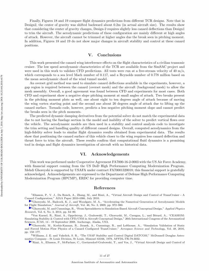
A CEASIOM-based model of the aircraft was generated and shown in Figure 1. Note that this is asimplified geometry of the aircraft and thus lacks the geometry refinements of final design. A CAD model ofthe TCR was created using CEASIOM-based geometry. This model is scaled 1:40 of the full aircraft for windtunnel experiments and has not the engine, aileron, and rudder surfaces. Parameters for the wind tunnelexperiment and the computational models of this work are provided in Table 2.
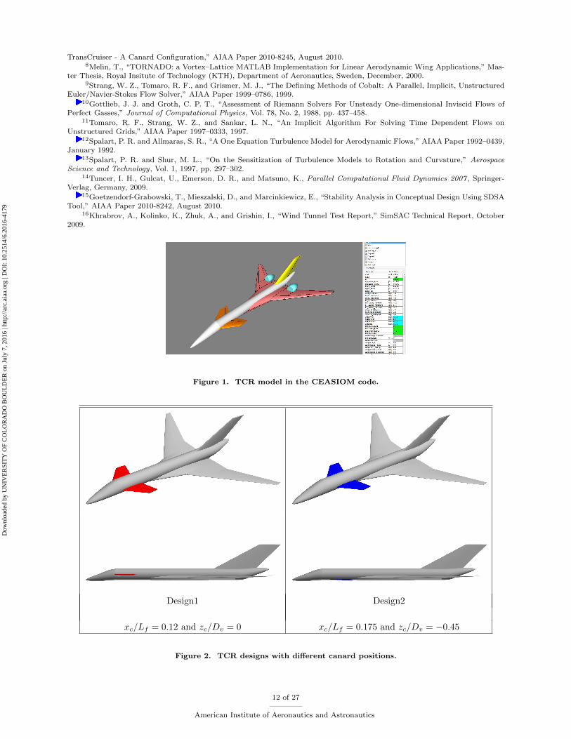
The original TCR model has a canard positioned at 0.12 of total fuselage length and at the mid fuselagesection. This is named “Design1” in this paper. A second design (named “Design2”) is considered as wellthat has canard positioned at 0.175 of total fuselage length and at a lower position than the original design.The CAD models of these designs were created in CEASIOM and shown in Figure 2. Full-geometry oversetgrids of the TCR designs (Design1 and Design2) were generated from these geometries. In these grids, abackground viscous grid was created around the fuselage, wing, and the tail. The canard viscous grids (rightand left) were generated individually as well. The surface grids are shown in Figure 3. The canard gridsare then overset to the background grid as illustrated in Figure 4 (a). Right- and left-side canard grids havefringe boundary surfaces (FBSs) that transfer information between grids. The overset grid module in Cobalt
7 of 27
American Institute of Aeronautics and Astronautics
Dow
nloa
ded
by U
NIV
ER
SIT
Y O
F C
OL
OR
AD
O B
OU
LD
ER
on
July
7, 2
016
| http
://ar
c.ai
aa.o
rg |
DO
I: 1
0.25
14/6
.201
6-41
79
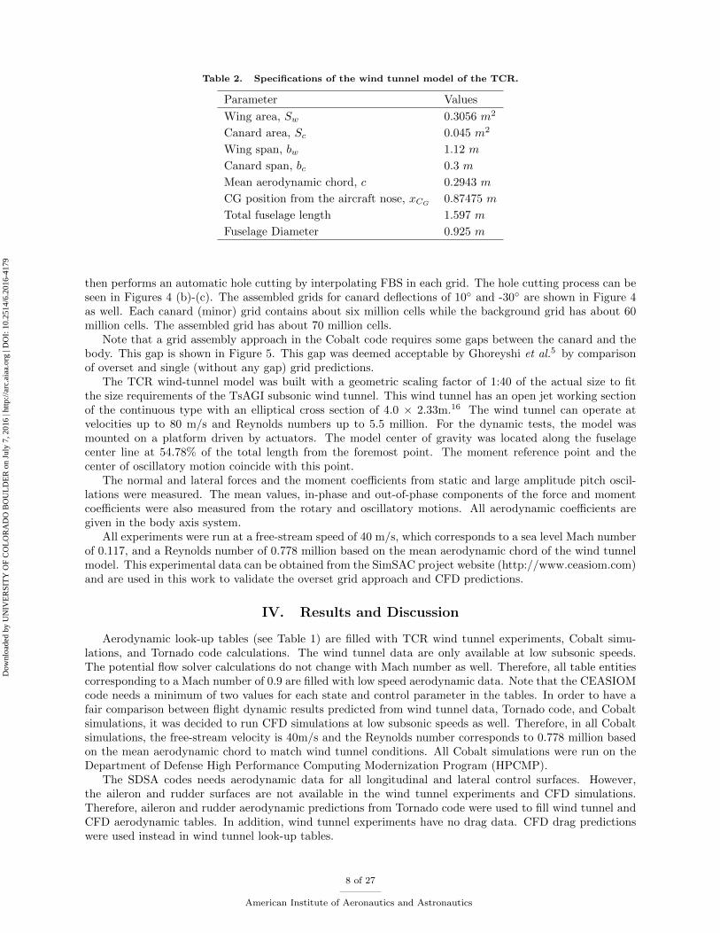
Table 2. Specifications of the wind tunnel model of the TCR.
Parameter Values
Wing area, Sw 0.3056 m2
Canard area, Sc 0.045 m2
Wing span, bw 1.12 m
Canard span, bc 0.3 m
Mean aerodynamic chord, c 0.2943 m
CG position from the aircraft nose, xCG0.87475 m
Total fuselage length 1.597 m
Fuselage Diameter 0.925 m
then performs an automatic hole cutting by interpolating FBS in each grid. The hole cutting process can beseen in Figures 4 (b)-(c). The assembled grids for canard deflections of 10◦ and -30◦ are shown in Figure 4as well. Each canard (minor) grid contains about six million cells while the background grid has about 60million cells. The assembled grid has about 70 million cells.
Note that a grid assembly approach in the Cobalt code requires some gaps between the canard and thebody. This gap is shown in Figure 5. This gap was deemed acceptable by Ghoreyshi et al.5 by comparisonof overset and single (without any gap) grid predictions.
The TCR wind-tunnel model was built with a geometric scaling factor of 1:40 of the actual size to fitthe size requirements of the TsAGI subsonic wind tunnel. This wind tunnel has an open jet working sectionof the continuous type with an elliptical cross section of 4.0 × 2.33m.16 The wind tunnel can operate atvelocities up to 80 m/s and Reynolds numbers up to 5.5 million. For the dynamic tests, the model wasmounted on a platform driven by actuators. The model center of gravity was located along the fuselagecenter line at 54.78% of the total length from the foremost point. The moment reference point and thecenter of oscillatory motion coincide with this point.
The normal and lateral forces and the moment coefficients from static and large amplitude pitch oscil-lations were measured. The mean values, in-phase and out-of-phase components of the force and momentcoefficients were also measured from the rotary and oscillatory motions. All aerodynamic coefficients aregiven in the body axis system.
All experiments were run at a free-stream speed of 40 m/s, which corresponds to a sea level Mach numberof 0.117, and a Reynolds number of 0.778 million based on the mean aerodynamic chord of the wind tunnelmodel. This experimental data can be obtained from the SimSAC project website (http://www.ceasiom.com)and are used in this work to validate the overset grid approach and CFD predictions.
IV. Results and Discussion
Aerodynamic look-up tables (see Table 1) are filled with TCR wind tunnel experiments, Cobalt simu-lations, and Tornado code calculations. The wind tunnel data are only available at low subsonic speeds.The potential flow solver calculations do not change with Mach number as well. Therefore, all table entitiescorresponding to a Mach number of 0.9 are filled with low speed aerodynamic data. Note that the CEASIOMcode needs a minimum of two values for each state and control parameter in the tables. In order to have afair comparison between flight dynamic results predicted from wind tunnel data, Tornado code, and Cobaltsimulations, it was decided to run CFD simulations at low subsonic speeds as well. Therefore, in all Cobaltsimulations, the free-stream velocity is 40m/s and the Reynolds number corresponds to 0.778 million basedon the mean aerodynamic chord to match wind tunnel conditions. All Cobalt simulations were run on theDepartment of Defense High Performance Computing Modernization Program (HPCMP).
The SDSA codes needs aerodynamic data for all longitudinal and lateral control surfaces. However,the aileron and rudder surfaces are not available in the wind tunnel experiments and CFD simulations.Therefore, aileron and rudder aerodynamic predictions from Tornado code were used to fill wind tunnel andCFD aerodynamic tables. In addition, wind tunnel experiments have no drag data. CFD drag predictionswere used instead in wind tunnel look-up tables.
8 of 27
American Institute of Aeronautics and Astronautics
Dow
nloa
ded
by U
NIV
ER
SIT
Y O
F C
OL
OR
AD
O B
OU
LD
ER
on
July
7, 2
016
| http
://ar
c.ai
aa.o
rg |
DO
I: 1
0.25
14/6
.201
6-41
79
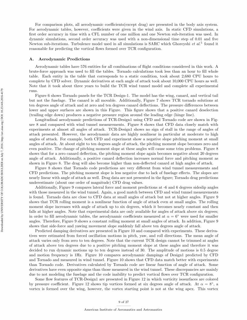
For comparison plots, all aerodynamic coefficients(except drag) are presented in the body axis system.For aerodynamic tables, however, coefficients were given in the wind axis. In static CFD simulations, afirst order accuracy in time with a CFL number of one million and one Newton sub-iteration was used. Indynamic simulations, second order accuracy was used with a non-dimensional time step of 0.01 and fiveNewton sub-iterations. Turbulence model used in all simulations is SARC which Ghoreyshi et al.5 found itreasonable for predicting the vortical flows formed over TCR configuration.
A. Aerodynamic Predictions
Aerodynamic tables have 576 entities for all combinations of flight conditions considered in this work. Abrute-force approach was used to fill the tables. Tornado calculations took less than an hour to fill wholetable. Each entity in the table that corresponds to a static condition, took about 2,680 CPU hours tocomplete by CFD solver. Dynamic derivatives at each angle of attack took about 10,000 CPU hours as well.Note that it took about three years to build the TCR wind tunnel model and complete all experimentalruns.
Figure 6 shows Tornado panels for the TCR Design-1. The model has the wing, canard, and vertical tailbut not the fuselage. The canard is all movable. Additionally, Figure 7 shows TCR tornado solutions atten degrees angle of attack and at zero and ten degrees canard deflections. The pressure differences betweenlower and upper surfaces are shown in this Figure. This figure shows that a positive canard deselection(trailing edge down) produces a negative pressure region around the leading edge (hinge line).
Longitudinal aerodynamic predictions of TCR-Design1 using CFD and Tornado code are shown in Fig-ure 8 and compared with wind tunnel measurements. Figure 8 shows that CFD data closely match withexperiments at almost all angles of attack. TCR-Design1 shows no sign of stall in the range of angles ofattack presented. However, the aerodynamic data are highly nonlinear in particular at moderate to highangles of attack. For example, both CFD and experiment show a negative slope pitching moment at smallangles of attack. At about eight to ten degrees angle of attack, the pitching moment slope becomes zero andeven positive. The change of pitching moment slope at these angles will cause some trim problems. Figure 8shows that for a zero canard deflection, the pitching moment slope again becomes negative about 20 degreesangle of attack. Additionally, a positive canard deflection increases normal force and pitching moment asshown in Figure 8. The drag will also become higher than non-deflected canard at high angles of attack.
Figure 8 shows that Tornado code predictions are very different from wind tunnel measurements andCFD predictions. The pitching moment slope is less negative due to lack of fuselage effects. The slopes arenearly linear with angle of attack as well. Drag data are not presented in the figure; Tornado drag predictionsunderestimate (about one order of magnitude) CFD drag values.
Additionally, Figure 9 compares lateral force and moment predictions at -6 and 6 degrees sideslip angleswith those measured in the wind tunnel. Again, a good match between CFD and wind tunnel measurementsis found. Tornado data are close to CFD data at small angles of attack but not at higher angles. Figure 9shows that TCR rolling moment is a nonlinear function of angle of attack even at small angles. The rollingmoment slope increases with angle of attack up to six degrees, which it becomes nearly constant and thenfalls at higher angles. Note that experimental data are only available for angles of attack above six degrees;in order to fill aerodynamic tables, the aerodynamic coefficients measured at α = 6◦ were used for smallerangles. Therefore, Figure 9 shows a constant rolling moment at small angles of attack. In addition, Figure 9shows that side-force and yawing movement slope suddenly fall above ten degrees angle of attack.
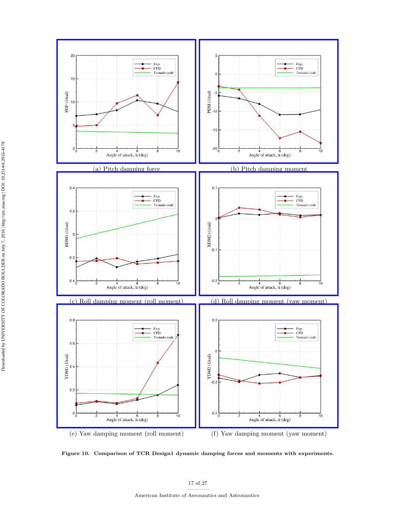
Predicted damping derivatives are presented in Figure 10 and compared with experiments. These deriva-tives were estimated from forced oscillation motions in pitch, yaw, and roll directions. The mean angle ofattack varies only from zero to ten degrees. Note that the current TCR design cannot be trimmed at anglesof attack above ten degrees due to a positive pitching moment slope at these angles and therefore it wasdecided to run dynamic motions up to ten degrees instead of 30. The amplitude of motions is 0.5 degreeand motion frequency is 1Hz. Figure 10 compares aerodynamic dampings of Design1 predicted by CFDand Tornado and measured in wind tunnel. Figure 10 shows that CFD data match better with experimentsthan Tornado code. Derivatives calculated by Tornado code are linear function of angle of attack. Somederivatives have even opposite signs than those measured in the wind tunnel. These discrepancies are mainlydue to not modeling the fuselage and the code inability to predict vortical flows over TCR configuration.
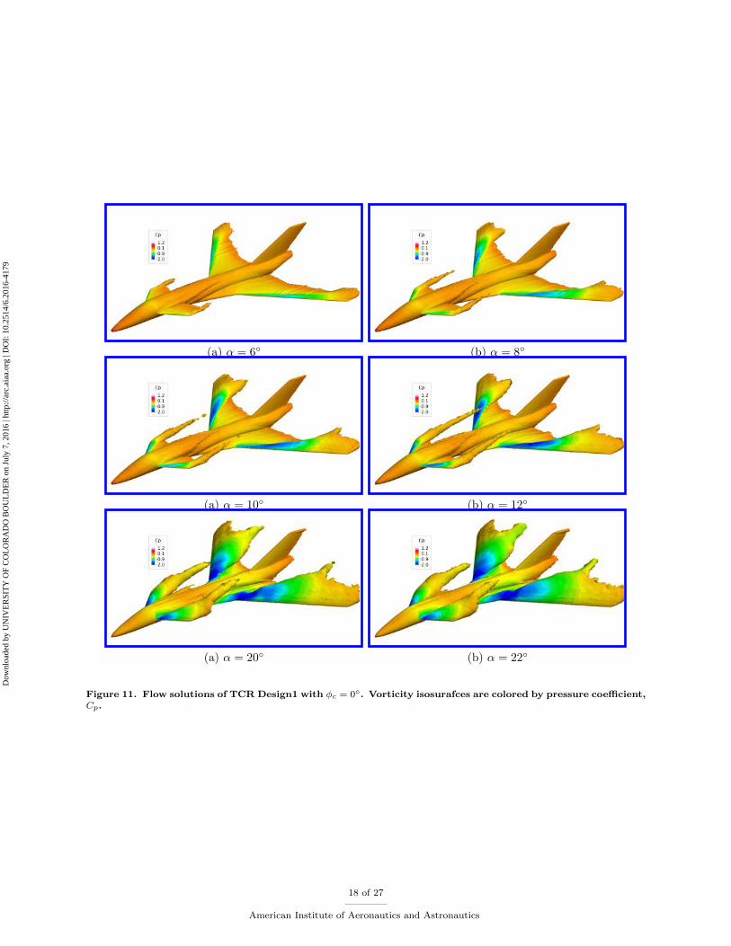
Some flow features of TCR-Design1 are presented in Figure 12 in which vorticity isosurfaces are coloredby pressure coefficient. Figure 12 shows tip vortices formed at six degrees angle of attack. At α = 8◦, avortex is formed over the wing, however, the vortex starting point is not at the wing apex. This vortex
9 of 27
American Institute of Aeronautics and Astronautics
Dow
nloa
ded
by U
NIV
ER
SIT
Y O
F C
OL
OR
AD
O B
OU
LD
ER
on
July
7, 2
016
| http
://ar
c.ai
aa.o
rg |
DO
I: 1
0.25
14/6
.201
6-41
79
induces negative pressures over the surface and causes the lift to increase. At higher angles of attack, thevortex starting point moves toward the wing apex which causes a positive increment in the pitching moment.At α = 10◦, the vortex starting point is at the wing apex. The canard vortex can be seen at this angle aswell. Further increase in the angle of attack does not move the vortex starting point, but vortices becomestronger and larger in size. At about α = 20◦, the inboard and outboard vortices interact and merge.
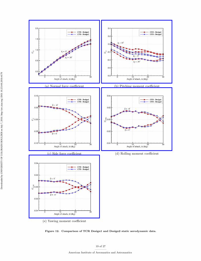
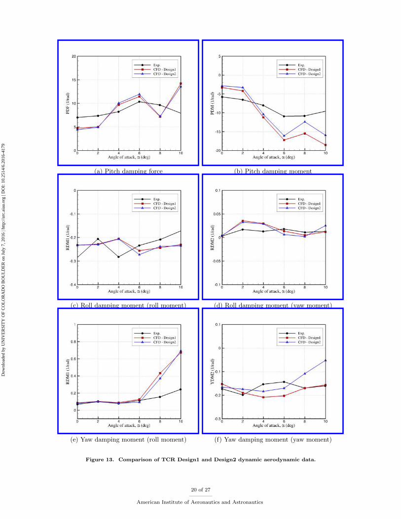
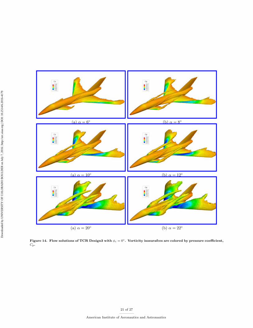
Static aerodynamics of both TCR designs are compared in Figure 12. The moment reference point is thesame in both simulations but the center of gravity of Design-1 is shifted backward in CEASIOM stabilityand control investigations (about 0.2m in full size plane). The results show that both designs have verysimilar coefficients at small angles of attack, except pitching and rolling moments that are slightly differentdue to different moment arms about the moment reference point. At higher angles, large differences can beseen between these designs. For example, Design-2 has bigger lateral force and moment coefficients up to 22degrees angle of attack. The pitching moment slopes are different as well. In addition, damping derivatives ofboth TCR designs are compared in Figure 13 which shows that both canard positions produce close dampingderivatives in particular at small angles of attack. Some of the flow features of TCR-Design2 are shown inFigure 14. The flow structures are similar to those found in Design-1, except that the forward-positionedcanard has stronger canard vortices.
In more detail, Figure 15 compares spanwise pressure coefficients of both designs at different chord-wiselocations and angles of attack. The pressure tap positions (six in total) are shown in Figure 15. Pressuredata of only four tap positions are shown in this figure; three located on the canard surface and one on thewing close to wing apex. At α = 6◦, a leading-edge vortex can be seen over the canard in both designs. Thisvortex induces a negative pressure over the canard upper surface, though the pressure data of both designsare very similar. No vortex presents over the wing at studied tap position and this angle of attack. Atα = 8◦, the canard vortex becomes stronger and the vortex axis moves inward. The vortex axis of Design-1shifts more than that of the vortex seen in Design-2. The wing outboard vortex can be seen at this angle ofattack as well. At this angle, both designs show very similar pressure data over wing.
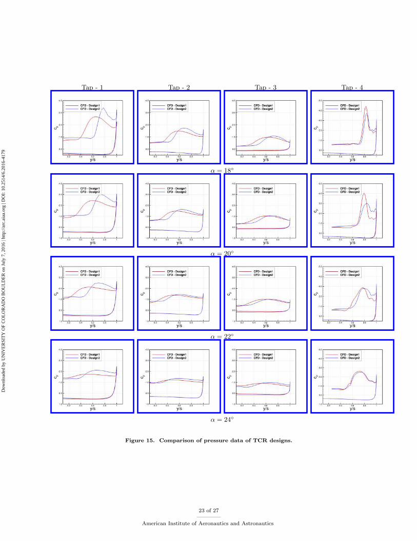
Figure 15 shows that canard vortex diameter increases with increasing angle of attack and the axis shiftsfurther inward. Differences between canard vortices in these designs become more visible at higher angles.Design-1 seems to have a stronger (wider) canard vortex than Design-2. However, the pressure coefficients onthe wing tap position are still close in both designs for angles of attack up to 18 degrees. At and above thisangle, Design-1 shows stronger outboard wing vortex than that predicted in Design-2. The vortex positionof Design-1 is more inward than Design-2 as well. The wing inboard vortex can be seen at this angle ofattack. At about α = 22◦, inboard and outboard vortices interact and then merge to form a single largevortex over the wing. At about α = 24◦, the canard vortex lifts up from the surface. For Design-1, vortexeffects are very small at all canard positions. For Design-2, small vortex effects can still be seen in showntap positions. Figure 15 shows that the differences between pressure coefficients over the wing between thesedesigns become smaller as the canard vortex effects become small.
B. Stability and Control Predictions
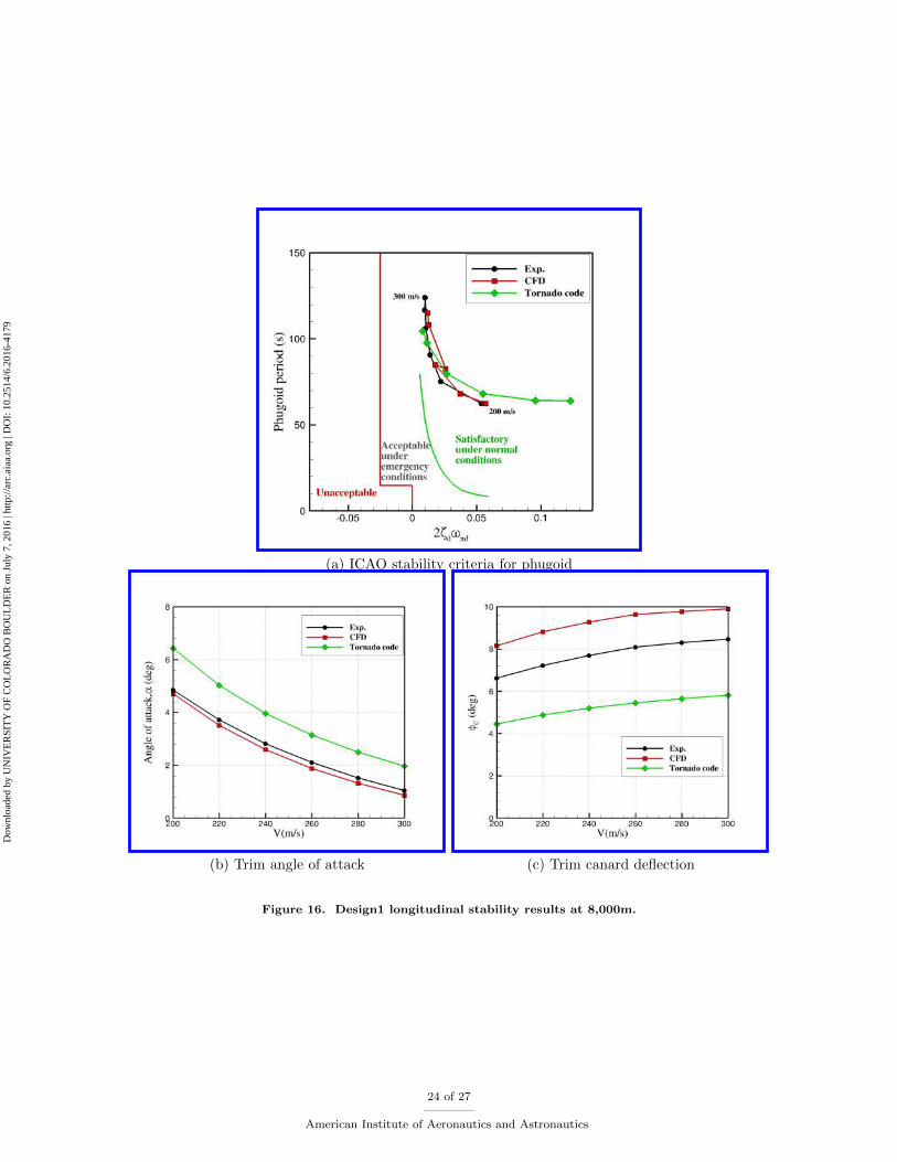
Aerodynamic tables of TCR-Design1 generated by wind tunnel, CFD simulations, and Tornado code wereinput to SDSA code to investigate the vehicle stability and handling qualities. The aircraft altitude was setat 8,000 m and speed was varied from 100 to 300 m/s. Note that these flight conditions correspond to muchhigher Mach numbers than the one used in generating aerodynamic models. Though, the aircraft can betrimmed using Tornado-generated tables, the SDSA predicted no trim states for the aircraft for speeds below200 m/s using wind tunnel and CFD tables. Figure 16 shows required angle of attack and canard deflectionto trim the aircraft at 8,000m and different speeds. Figure shows that required angle of attack increases atsmall speeds. At some angle of attack, the pitching moment slopes become zero or positive and therefore notrim state can be obtained. However, Tornado pitching moment slope are negative for considered angles ofattack and it still predicts a trim point at wider range of air speeds.
In more detail, Figure 16 shows that predictions from Tornado code require larger angles of attack andless canard deflections to trim aircraft compared with wind tunnel and CFD predictions. All models predictsatisfactory phugoid stability performance, however, Tornado tables predict much larger damping ratios thanexperimental and CFD data.
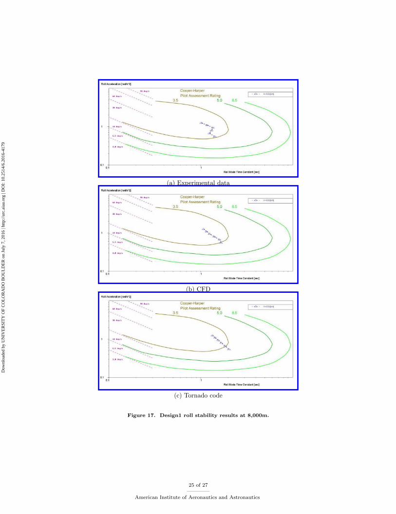
Figure 17 also compares roll stability results calculated in the SDSA code using different aerodynamictables. The results seems similar to each other from all three aerodynamic sources, but wind tunnel andCFD show more nonlinear trends than Tornado predictions.
10 of 27
American Institute of Aeronautics and Astronautics
Dow
nloa
ded
by U
NIV
ER
SIT
Y O
F C
OL
OR
AD
O B
OU
LD
ER
on
July
7, 2
016
| http
://ar
c.ai
aa.o
rg |
DO
I: 1
0.25
14/6
.201
6-41
79
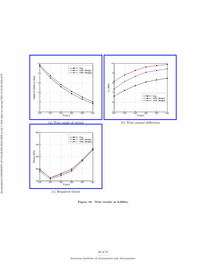
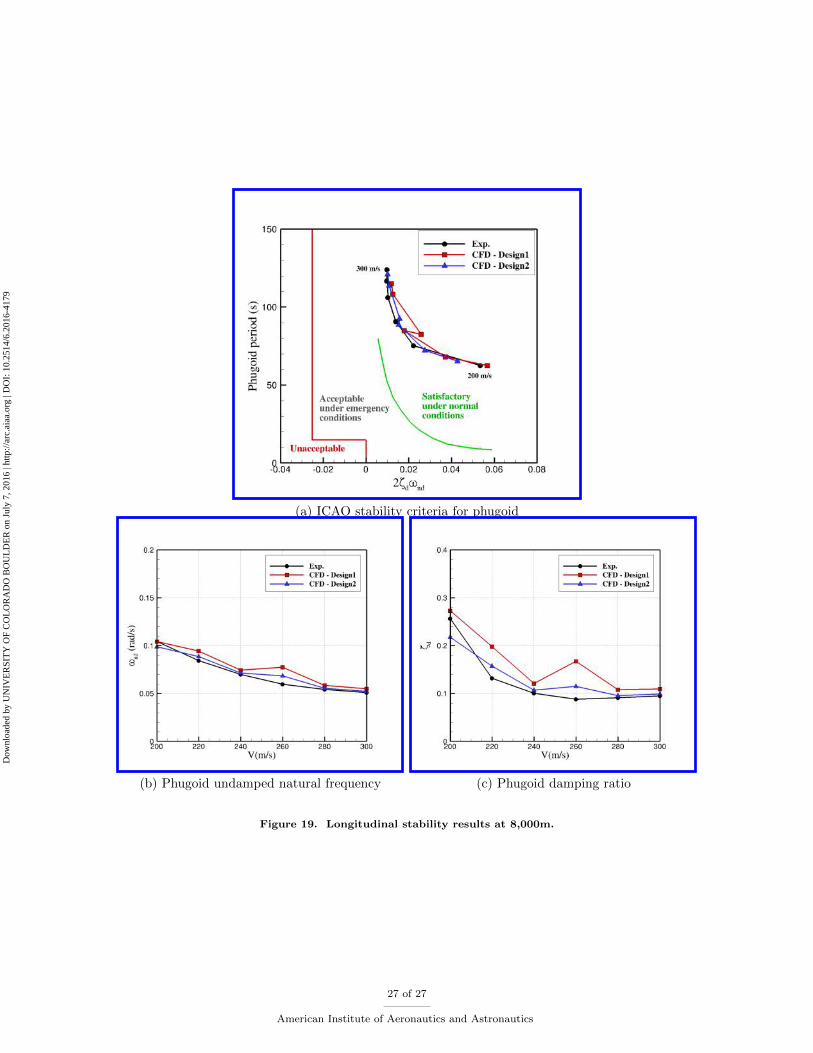
Finally, Figures 18 and 19 compare flight dynamics predictions from different TCR designs. Note that inDesign2, the center of gravity was shifted backward about 0.2m (in actual aircraft size). The results showthat considering the center of gravity changes, Design-2 requires slightly less canard deflections than Design1to trim the aircraft. The aerodynamic predictions of these configuration are mainly different at high anglesof attack. However, the aircraft cannot be trimmed at higher angles due the break seen in pitching moment.In addition, Figures 18 and 19 do not show major changes in aircraft stability and control at these canardpositions.
V. Conclusions
This work presented the canard wing interference effects on the flight characteristics of a civilian transoniccruiser. The low speed aerodynamic characteristics of the TCR are available from the SimSAC project andwere used in this work to validate CFD predictions. All tests were run at a free-stream velocity of 40 m/s,which corresponds to a sea level Mach number of 0.117, and a Reynolds number of 0.778 million based onthe mean aerodynamic chord of the wind tunnel model.
An overset grid method was used to simulate canard deflections available in the experiments, however, agap region is required between the canard (overset mesh) and the aircraft (background mesh) to allow themesh assembly. Overall, a good agreement was found between CFD and experiments for most cases. BothCFD and experiment show a negative slope pitching moment at small angles of attack. Two breaks presentin the pitching moment plots as well, one about eight to ten degrees angle of attack because of movingthe wing vortex starting point and the second one about 20 degrees angle of attack due to lifting up thecanard surface. Tornado code, however, predicts a less negative pitching moment slope and cannot predictthe breaks seen in the pitch moments.
The predicted dynamic damping derivatives from the potential solver do not match the experimental datadue to not having the fuselage section in the model and inability of the solver to predict vortical flows overthe vehicle. The aerodynamic models are then used in a stability and control analysis code to investigatethe trim setting and handling quality of different canard designs. Overall, computed aerodynamics from thehigh-fidelity solver leads to similar flight dynamics results obtained from experimental data. The resultsshow that positioning the canard surface of this vehicle closer to the wing requires less canard deflection andthrust force to trim the aircraft. These results confirm that computational fluid dynamics is a promisingtool in design and flight dynamics investigation of aircraft with no historical data.
VI. Acknowledgements
This work was performed under Cooperative Agreement FA7000-16-2-0003 with the US Air Force Academy,with financial support coming from the US DoD High Performance Computing Modernization Program.Mehdi Ghoreyshi is supported by USAFA under contract FA70001320018; this financial support is gratefullyacknowledged. Acknowledgements are expressed to the Department of Defense High Performance ComputingModernization Program (HPCMP), ERDC for providing computer time.
References
1Eliasson, P., V. J., Da Ronch, A., Zhang, M., and Rizzi, A., “Virtual Aircraft Design and Control of TransCruiser - ACanard Configuration,” AIAA Paper 2010-4366, July 2010.
2Ghoreyshi, M., Badcock, K. J., and Woodgate, M. A., “Accelerating the Numerical Generation of Aerodynamic Modelsfor Flight Simulation,” Journal of Aircraft , Vol. 46, No. 3, 2009, pp. 972–980.
3Ghoreyshi, M. and Cummings, R., “From Spreadsheets to Simulation-Based Aircraft Conceptual Design,” Applied PhysicsResearch, Vol. 6, No. 3, 2014, pp. 64–80.
4Von Kaenel, R., Rizzi, A., Oppelstrup, J., Grabowski, T., Ghoreyshi, M., Cavagna, L., and Berard, A., “CEASIOM:Simulating Stability & Control with CFD/CSM in Aircraft Conceptual Design,” 26th International Congress of the AeronauticalSciences, ICAS, 14 - 19 September 2008, Anchorage, Alaska, USA.
5Ghoreyshi, M., Korkis-Kanaan, R., Jirasek, A., Cummings, R., and Lofthouse, A., “Simulation Validation of Staticand Forced Motion Flow Physics of a Canard Configured TransCruiser,” Aerospace Science and Technology, Vol. 48, 2016,pp. 158–177.
6Williams, J. E. and Vukelich, S. R., “The USAF Stability and Control Digital DATCOM,” McDonnell Douglas Astro-nautics Company - St Louis Division, St Louis, Missouri 63166, 1979, AFFDL-TR-79-3032.
7Rizzi, A., Eliasson, P., McFarlane, C., Goetzendorf-Grabowski, T., and Vos, J., “Virtual Aircraft Design and Control of
11 of 27
American Institute of Aeronautics and Astronautics
Dow
nloa
ded
by U
NIV
ER
SIT
Y O
F C
OL
OR
AD
O B
OU
LD
ER
on
July
7, 2
016
| http
://ar
c.ai
aa.o
rg |
DO
I: 1
0.25
14/6
.201
6-41
79
TransCruiser - A Canard Configuration,” AIAA Paper 2010-8245, August 2010.8Melin, T., “TORNADO: a Vortex–Lattice MATLAB Implementation for Linear Aerodynamic Wing Applications,” Mas-
ter Thesis, Royal Insitute of Technology (KTH), Department of Aeronautics, Sweden, December, 2000.9Strang, W. Z., Tomaro, R. F., and Grismer, M. J., “The Defining Methods of Cobalt: A Parallel, Implicit, Unstructured
Euler/Navier-Stokes Flow Solver,” AIAA Paper 1999–0786, 1999.10Gottlieb, J. J. and Groth, C. P. T., “Assessment of Riemann Solvers For Unsteady One-dimensional Inviscid Flows of
Perfect Gasses,” Journal of Computational Physics, Vol. 78, No. 2, 1988, pp. 437–458.11Tomaro, R. F., Strang, W. Z., and Sankar, L. N., “An Implicit Algorithm For Solving Time Dependent Flows on
Unstructured Grids,” AIAA Paper 1997–0333, 1997.12Spalart, P. R. and Allmaras, S. R., “A One Equation Turbulence Model for Aerodynamic Flows,” AIAA Paper 1992–0439,
January 1992.13Spalart, P. R. and Shur, M. L., “On the Sensitization of Turbulence Models to Rotation and Curvature,” Aerospace
Science and Technology, Vol. 1, 1997, pp. 297–302.14Tuncer, I. H., Gulcat, U., Emerson, D. R., and Matsuno, K., Parallel Computational Fluid Dynamics 2007 , Springer-
Verlag, Germany, 2009.15Goetzendorf-Grabowski, T., Mieszalski, D., and Marcinkiewicz, E., “Stability Analysis in Conceptual Design Using SDSA
Tool,” AIAA Paper 2010-8242, August 2010.16Khrabrov, A., Kolinko, K., Zhuk, A., and Grishin, I., “Wind Tunnel Test Report,” SimSAC Technical Report, October
2009.
Figure 1. TCR model in the CEASIOM code.
Design1 Design2
xc/Lf = 0.12 and zc/Dv = 0 xc/Lf = 0.175 and zc/Dv = −0.45
Figure 2. TCR designs with different canard positions.
12 of 27
American Institute of Aeronautics and Astronautics
Dow
nloa
ded
by U
NIV
ER
SIT
Y O
F C
OL
OR
AD
O B
OU
LD
ER
on
July
7, 2
016
| http
://ar
c.ai
aa.o
rg |
DO
I: 1
0.25
14/6
.201
6-41
79
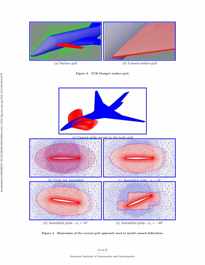
(a) Surface grid (b) Canard surface grid
Figure 3. TCR Design1 surface grid.
(a) Canard grids overset to the body grid
(b) Grids not assembled (c) Assembled grids - φc = 0◦
(d) Assembled grids - φc = 10◦ (e) Assembled grids - φc = −30◦
Figure 4. Illustration of the overset grid approach used to model canard deflections.
13 of 27
American Institute of Aeronautics and Astronautics
Dow
nloa
ded
by U
NIV
ER
SIT
Y O
F C
OL
OR
AD
O B
OU
LD
ER
on
July
7, 2
016
| http
://ar
c.ai
aa.o
rg |
DO
I: 1
0.25
14/6
.201
6-41
79
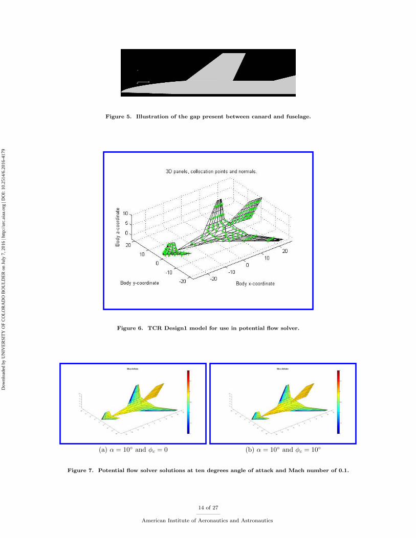
Figure 5. Illustration of the gap present between canard and fuselage.
Figure 6. TCR Design1 model for use in potential flow solver.
(a) α = 10◦ and φc = 0 (b) α = 10◦ and φc = 10◦
Figure 7. Potential flow solver solutions at ten degrees angle of attack and Mach number of 0.1.
14 of 27
American Institute of Aeronautics and Astronautics
Dow
nloa
ded
by U
NIV
ER
SIT
Y O
F C
OL
OR
AD
O B
OU
LD
ER
on
July
7, 2
016
| http
://ar
c.ai
aa.o
rg |
DO
I: 1
0.25
14/6
.201
6-41
79
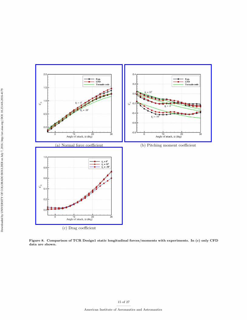
(a) Normal force coefficient (b) Pitching moment coefficient
(c) Drag coefficient
Figure 8. Comparison of TCR Design1 static longitudinal forces/moments with experiments. In (c) only CFDdata are shown.
15 of 27
American Institute of Aeronautics and Astronautics
Dow
nloa
ded
by U
NIV
ER
SIT
Y O
F C
OL
OR
AD
O B
OU
LD
ER
on
July
7, 2
016
| http
://ar
c.ai
aa.o
rg |
DO
I: 1
0.25
14/6
.201
6-41
79
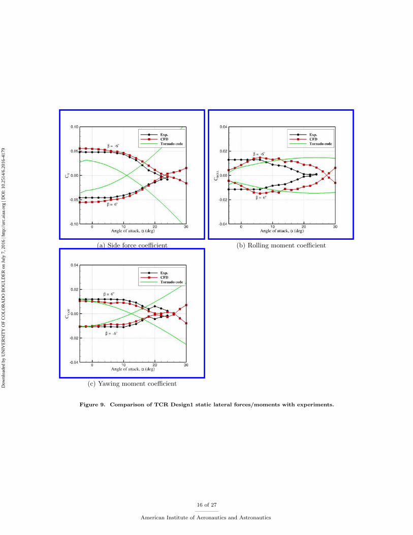
(a) Side force coefficient (b) Rolling moment coefficient
(c) Yawing moment coefficient
Figure 9. Comparison of TCR Design1 static lateral forces/moments with experiments.
16 of 27
American Institute of Aeronautics and Astronautics
Dow
nloa
ded
by U
NIV
ER
SIT
Y O
F C
OL
OR
AD
O B
OU
LD
ER
on
July
7, 2
016
| http
://ar
c.ai
aa.o
rg |
DO
I: 1
0.25
14/6
.201
6-41
79
(a) Pitch damping force (b) Pitch damping moment
(c) Roll damping moment (roll moment) (d) Roll damping moment (yaw moment)
(e) Yaw damping moment (roll moment) (f) Yaw damping moment (yaw moment)
Figure 10. Comparison of TCR Design1 dynamic damping forces and moments with experiments.
17 of 27
American Institute of Aeronautics and Astronautics
Dow
nloa
ded
by U
NIV
ER
SIT
Y O
F C
OL
OR
AD
O B
OU
LD
ER
on
July
7, 2
016
| http
://ar
c.ai
aa.o
rg |
DO
I: 1
0.25
14/6
.201
6-41
79
(a) α = 6◦ (b) α = 8◦
(a) α = 10◦ (b) α = 12◦
(a) α = 20◦ (b) α = 22◦
Figure 11. Flow solutions of TCR Design1 with φc = 0◦. Vorticity isosurafces are colored by pressure coefficient,Cp.
18 of 27
American Institute of Aeronautics and Astronautics
Dow
nloa
ded
by U
NIV
ER
SIT
Y O
F C
OL
OR
AD
O B
OU
LD
ER
on
July
7, 2
016
| http
://ar
c.ai
aa.o
rg |
DO
I: 1
0.25
14/6
.201
6-41
79
(a) Normal force coefficient (b) Pitching moment coefficient
(c) Side force coefficient (d) Rolling moment coefficient
(e) Yawing moment coefficient
Figure 12. Comparison of TCR Design1 and Design2 static aerodynamic data.
19 of 27
American Institute of Aeronautics and Astronautics
Dow
nloa
ded
by U
NIV
ER
SIT
Y O
F C
OL
OR
AD
O B
OU
LD
ER
on
July
7, 2
016
| http
://ar
c.ai
aa.o
rg |
DO
I: 1
0.25
14/6
.201
6-41
79
(a) Pitch damping force (b) Pitch damping moment
(c) Roll damping moment (roll moment) (d) Roll damping moment (yaw moment)
(e) Yaw damping moment (roll moment) (f) Yaw damping moment (yaw moment)
Figure 13. Comparison of TCR Design1 and Design2 dynamic aerodynamic data.
20 of 27
American Institute of Aeronautics and Astronautics
Dow
nloa
ded
by U
NIV
ER
SIT
Y O
F C
OL
OR
AD
O B
OU
LD
ER
on
July
7, 2
016
| http
://ar
c.ai
aa.o
rg |
DO
I: 1
0.25
14/6
.201
6-41
79
(a) α = 6◦ (b) α = 8◦
(a) α = 10◦ (b) α = 12◦
(a) α = 20◦ (b) α = 22◦
Figure 14. Flow solutions of TCR Design3 with φc = 0◦. Vorticity isosurafces are colored by pressure coefficient,Cp.
21 of 27
American Institute of Aeronautics and Astronautics
Dow
nloa
ded
by U
NIV
ER
SIT
Y O
F C
OL
OR
AD
O B
OU
LD
ER
on
July
7, 2
016
| http
://ar
c.ai
aa.o
rg |
DO
I: 1
0.25
14/6
.201
6-41
79
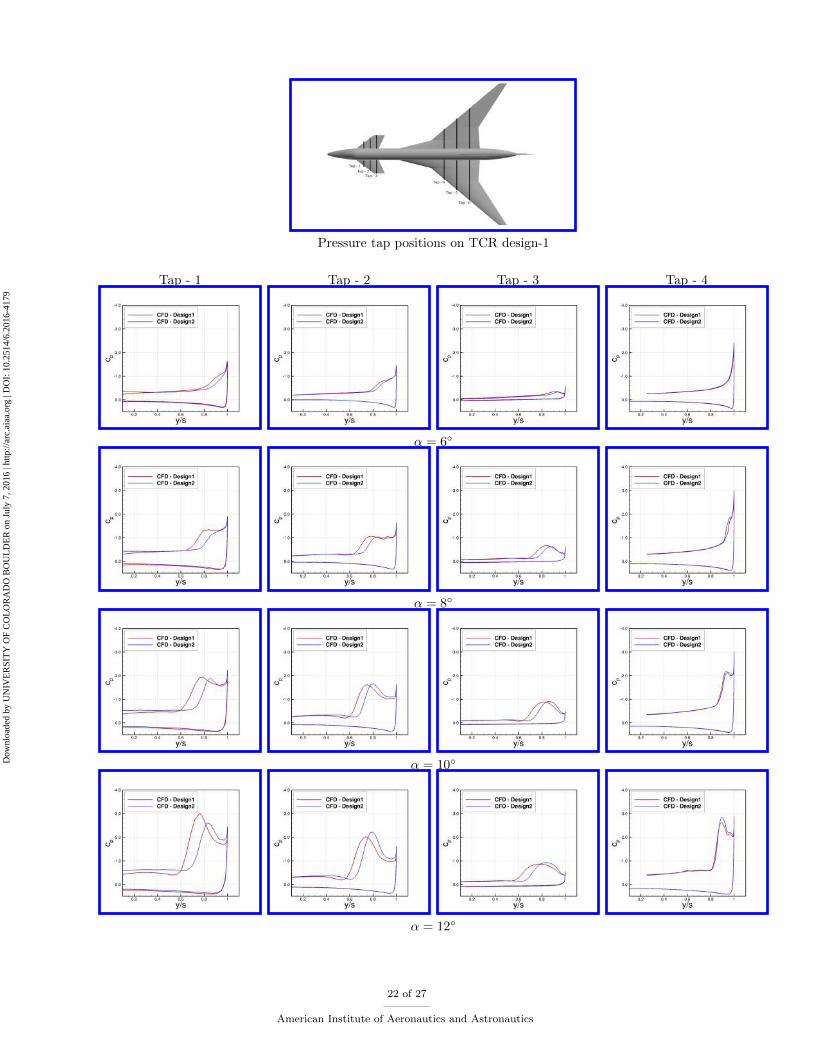
Pressure tap positions on TCR design-1
Tap - 1 Tap - 2 Tap - 3 Tap - 4
α = 6◦
α = 8◦
α = 10◦
α = 12◦
22 of 27
American Institute of Aeronautics and Astronautics
Dow
nloa
ded
by U
NIV
ER
SIT
Y O
F C
OL
OR
AD
O B
OU
LD
ER
on
July
7, 2
016
| http
://ar
c.ai
aa.o
rg |
DO
I: 1
0.25
14/6
.201
6-41
79
Tap - 1 Tap - 2 Tap - 3 Tap - 4
α = 18◦
α = 20◦
α = 22◦
α = 24◦
Figure 15. Comparison of pressure data of TCR designs.
23 of 27
American Institute of Aeronautics and Astronautics
Dow
nloa
ded
by U
NIV
ER
SIT
Y O
F C
OL
OR
AD
O B
OU
LD
ER
on
July
7, 2
016
| http
://ar
c.ai
aa.o
rg |
DO
I: 1
0.25
14/6
.201
6-41
79
(a) ICAO stability criteria for phugoid
(b) Trim angle of attack (c) Trim canard deflection
Figure 16. Design1 longitudinal stability results at 8,000m.
24 of 27
American Institute of Aeronautics and Astronautics
Dow
nloa
ded
by U
NIV
ER
SIT
Y O
F C
OL
OR
AD
O B
OU
LD
ER
on
July
7, 2
016
| http
://ar
c.ai
aa.o
rg |
DO
I: 1
0.25
14/6
.201
6-41
79
(a) Experimental data
(b) CFD
(c) Tornado code
Figure 17. Design1 roll stability results at 8,000m.
25 of 27
American Institute of Aeronautics and Astronautics
Dow
nloa
ded
by U
NIV
ER
SIT
Y O
F C
OL
OR
AD
O B
OU
LD
ER
on
July
7, 2
016
| http
://ar
c.ai
aa.o
rg |
DO
I: 1
0.25
14/6
.201
6-41
79
(a) Trim angle of attack (b) Trim canard deflection
(c) Required thrust
Figure 18. Trim results at 8,000m.
26 of 27
American Institute of Aeronautics and Astronautics
Dow
nloa
ded
by U
NIV
ER
SIT
Y O
F C
OL
OR
AD
O B
OU
LD
ER
on
July
7, 2
016
| http
://ar
c.ai
aa.o
rg |
DO
I: 1
0.25
14/6
.201
6-41
79
(a) ICAO stability criteria for phugoid
(b) Phugoid undamped natural frequency (c) Phugoid damping ratio
Figure 19. Longitudinal stability results at 8,000m.
27 of 27
American Institute of Aeronautics and Astronautics
Dow
nloa
ded
by U
NIV
ER
SIT
Y O
F C
OL
OR
AD
O B
OU
LD
ER
on
July
7, 2
016
| http
://ar
c.ai
aa.o
rg |
DO
I: 1
0.25
14/6
.201
6-41
79