Canonical Correlation Forests

Tom Rainforth TWGR@ROBOTS.OX.AC.UKDepartment of Engineering ScienceUniversity of OxfordParks Road, Oxford, OX1 3PJ, UK

Frank Wood FWOOD@ROBOTS.OX.AC.UK

Department of Engineering ScienceUniversity of OxfordParks Road, Oxford, OX1 3PJ, UK

AbstractWe introduce canonical correlation forests (CCFs), a new decision tree ensemble method for clas-sification and regression. Individual canonical correlation trees are binary decision trees with hy-perplane splits based on local canonical correlation coefficients calculated during training. Unlikeaxis-aligned alternatives, the decision surfaces of CCFs are not restricted to the coordinate systemof the inputs features and therefore more naturally represent data with correlated inputs. CCFsnaturally accommodate multiple outputs, provide a similar computational complexity to randomforests, and inherit their impressive robustness to the choice of input parameters. As part of theCCF training algorithm, we also introduce projection bootstrapping, a novel alternative to bag-ging for oblique decision tree ensembles which maintains use of the full dataset in selecting splitpoints, often leading to improvements in predictive accuracy. Our experiments show that, evenwithout parameter tuning, CCFs out-perform axis-aligned random forests and other state-of-the-arttree ensemble methods on both classification and regression problems, delivering both improvedpredictive accuracy and faster training times. We further show that they outperform all of the 179classifiers considered in a recent extensive survey.

Keywords: random forests, canonical correlation analysis, classification, regression, multipleoutput prediction

1. Introduction

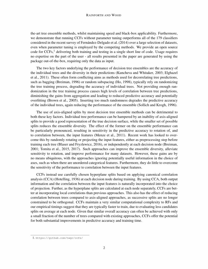
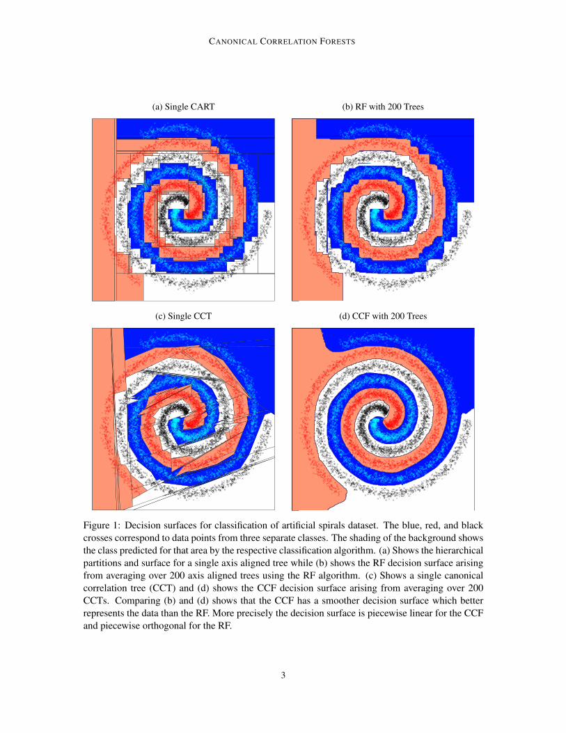
Decision tree ensemble methods such as random forests (RF) (Breiman, 2001), extremely random-ized trees (Geurts et al., 2006a), and boosted decision trees (Friedman, 2001) are widely employedmethods for classification and regression due to their scalability, fast out of sample prediction, andtendency to require little parameter tuning. In many cases, they give predictive performance closeto, or even equalling, state of the art when used in an out-of-the-box fashion (Fernandez-Delgadoet al., 2014), i.e. when parameters are set to default values. The individual trees used in suchalgorithms are, however, typically axis-aligned, restricting the ensemble decision surfaces to bepiecewise axis-aligned, even when there is little evidence for this in the data. Canonical correlationforests (CCFs) overcome this problem by instead using carefully chosen hyperplane splits, leadingto a more powerful classifier (or regressor) that naturally incorporates correlation between the fea-tures, an example for which shown in Figure 1. In this paper we demonstrate that this innovationregularly leads to a significant increase in out-of-sample predictive accuracy over previous state-of-

c©2017 Tom Rainforth and Frank Wood.

arX

iv:1

507.

0544

4v6

[st

at.M

L]

9 A

ug 2

017

RAINFORTH AND WOOD

the-art tree ensemble methods, whilst maintaining speed and black-box applicability. Furthermore,we demonstrate that running CCFs without parameter tuning outperforms all of the 179 classifiersconsidered in the recent survey of Fernandez-Delgado et al. (2014) over a large selection of datasets,even when parameter tuning is employed by the competing methods. We provide an open sourcecode for CCFs,1 delivering both training and testing in a single short line of code. Usage requiresno expertise on the part of the user - all results presented in the paper are generated by using thepackage out-of-the-box, requiring only the data as input.

The two key factors underlying the performance of decision tree ensembles are the accuracy ofthe individual trees and the diversity in their predictions (Kuncheva and Whitaker, 2003; Elghazelet al., 2011). These often form conflicting aims as methods used for decorrelating tree predictions,such as bagging (Breiman, 1996) or random subspacing (Ho, 1998), typically rely on randomizingthe tree training process, degrading the accuracy of individual trees. Not providing enough ran-domization in the tree training process causes high levels of correlation between tree predictions,diminishing the gains from aggregation and leading to reduced predictive accuracy and potentiallyoverfitting (Brown et al., 2005). Inserting too much randomness degrades the predictive accuracyof the individual trees, again reducing the performance of the ensemble (Sollich and Krogh, 1996).

The use of axis-aligned splits by most decision tree ensemble methods can be detrimental toboth these key factors. Individual tree performance can be hampered by an inability of axis-alignedsplits to provide a good representation of the true decision surface, while the smaller set of possiblesplits reduces the ensemble diversity. The effect of the former on the ensemble performance canbe particularly pronounced, resulting in sensitivity in the predictive accuracy to rotation of, andto correlation between, the input features (Menze et al., 2011). Recent work has looked to over-come this by randomly rotating or projecting the input features, either as preprocessing step beforetraining each tree (Blaser and Fryzlewicz, 2016), or independently at each decision node (Breiman,2001; Tomita et al., 2015, 2017). Such approaches can improve the ensemble diversity, alleviatesensitivity to rotation, and improve performance for many datasets. However, these gains are byno means ubiquitous, with the approaches ignoring potentially useful information in the choice ofaxes, such as when there are unordered categorical features. Furthermore, they do little to overcomethe sensitivity of the performance to correlation between the input features.

CCFs instead use carefully chosen hyperplane splits based on applying canonical correlationanalysis (CCA) (Hotelling, 1936) at each decision node during training. By using CCA, both outputinformation and the correlation between the input features is naturally incorporated into the choiceof projection. Further, as the hyperplane splits are calculated at each node separately, CCFs are bet-ter at incorporating local correlations than previous approaches. This also has the effect of reducingcorrelation between trees compared to axis-aligned approaches, as successive splits are no longerconstrained to be orthogonal. CCFs maintain a very similar computational complexity to RFs andour empirical timings suggest that they are typically faster to train, due to evaluating less candidatessplits on average at each node. Given that similar overall accuracy can often be achieved with onlya small fraction of the number of trees compared with existing approaches, CCFs offer the potentialfor both substantial improvements in predictive accuracy and training time.

1. https://github.com/twgr/ccfs/

2

CANONICAL CORRELATION FORESTS

(a) Single CART (b) RF with 200 Trees

(c) Single CCT (d) CCF with 200 Trees

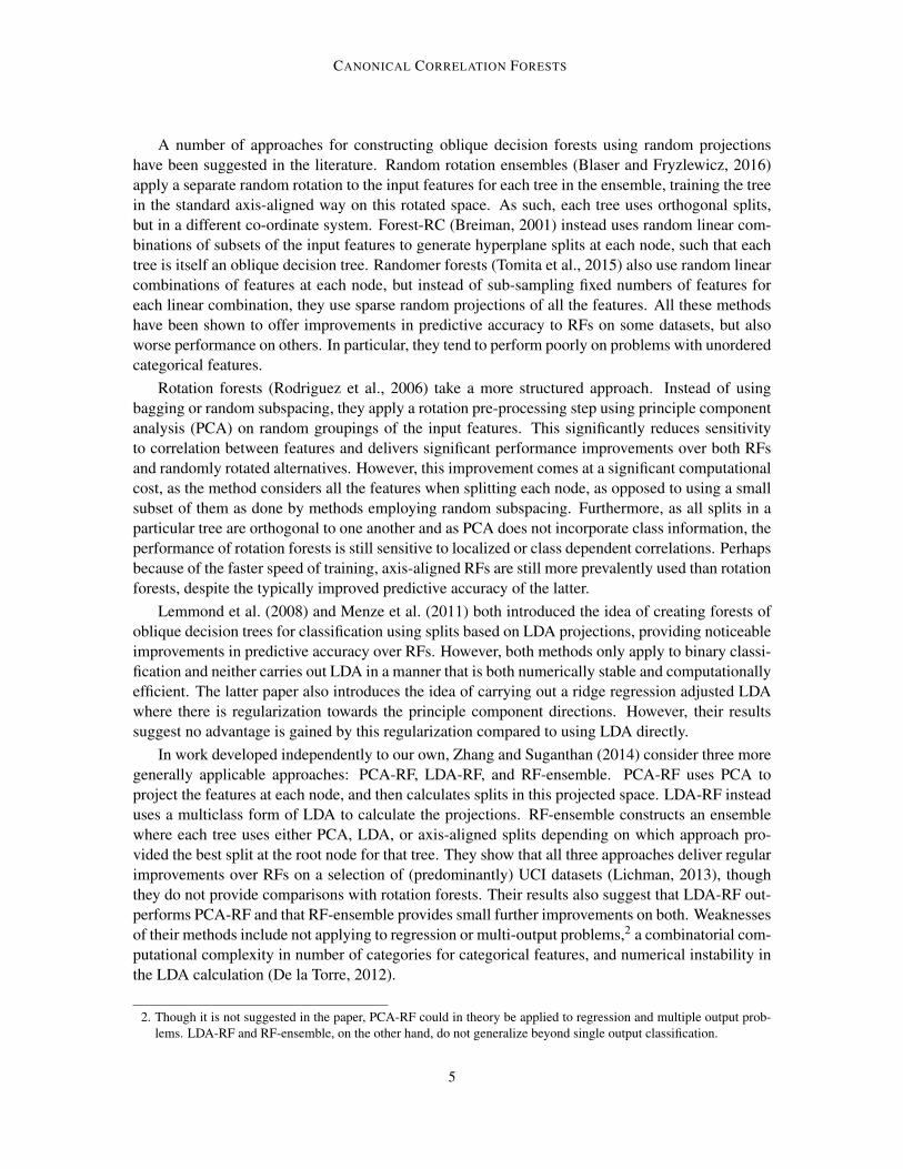
Figure 1: Decision surfaces for classification of artificial spirals dataset. The blue, red, and blackcrosses correspond to data points from three separate classes. The shading of the background showsthe class predicted for that area by the respective classification algorithm. (a) Shows the hierarchicalpartitions and surface for a single axis aligned tree while (b) shows the RF decision surface arisingfrom averaging over 200 axis aligned trees using the RF algorithm. (c) Shows a single canonicalcorrelation tree (CCT) and (d) shows the CCF decision surface arising from averaging over 200CCTs. Comparing (b) and (d) shows that the CCF has a smoother decision surface which betterrepresents the data than the RF. More precisely the decision surface is piecewise linear for the CCFand piecewise orthogonal for the RF.

3

RAINFORTH AND WOOD

2. Background

2.1 Decision Tree Ensembles

A decision tree is a predictive model that imposes sequential divisions of an input space to forma set of partitions known as leafs, each containing a local classification or regression model. Out-of-sample prediction is performed by using the partitioning to assign each new input to a particularleaf and then using the corresponding local predictive model. Typically, the leaf models are taken tobe independent of each other and the outputs are assumed to be independent of input features giventhe leaf assignments.

Classical decision tree learning algorithms work in a greedy top down fashion, exhaustivelysearching the space of unique axis-aligned splits and choosing the best based on a splitting criterion,such as the Gini gain or information gain used in CART (Breiman et al., 1984) and C4.5 (Quinlan,2014) respectively. Once a split is chosen, it is used to assigned each data point in the training set toone of the newly generated child nodes. The process then recurses in a self-similar manner for eachof the child nodes, continuing until no further split is advantageous or some user-set limit is reachedfor all the generated nodes. For classification with continuous features this typically only occursonce each leaf is “pure,” containing only data points of a single class. When used as individualclassifiers or regressors, trees are usually “pruned” after being grown to prevent overfitting. This isa regularization process which involves collapsing sub-branches of the tree to single leaf nodes.

It was established by Ho (1995) that combining individual trees to form a decision tree en-semble, or forest, can simultaneously improve predictive performance and provide regularizationagainst overfitting without the need for pruning. In a forest, each tree is separately trained, withprediction based on averaging predictions from the individual trees, resulting in a predictor that typ-ically outperforms any single constituent tree (Rokach, 2010). As classical decision tree algorithmsare deterministic procedures, such combination requires the introduction of probabilistic elementsinto the generative process to prevent identical trees. One possible approach, the random subspacemethod (Ho, 1995, 1998), involves only searching splits using a randomly selected subset of thefeatures at each node. Bagging (Breiman, 1996) instead trains each tree on a bootstrap sampleof the original dataset. Arguably the most widely used decision tree ensemble approach, randomforests (RFs) (Breiman, 2001), combines these randomization approaches, providing improved out-of-sample predictive performance to using either approach in isolation.

2.2 Oblique Decision Trees and Forests

Oblique decision trees (ODTs) extend classical decision trees by splitting using linear combinationsof the available features. Some algorithms such as OC1 (Murthy et al., 1994) attempt to directlyoptimize for the hyperplane representing the best split, while others, such as functional trees (Gama,2004) and QUEST (Loh and Shih, 1997), carry out a linear discriminant analysis (LDA) (Fisher,1936; Rao, 1948) to find a projection which optimizes the discriminant criterion and then search overpossible splits in this projected space. Although ODTs generally produce better results than axisaligned trees, many existing algorithms suffer from a number of common issues such as a failure toeffectively deal with multiple classes, numerical instability or significant increase in computationalcost compared with an axis aligned alternative. Many also only apply to classification problems anddo not naturally extend to regression or multiple output settings.

4

CANONICAL CORRELATION FORESTS

A number of approaches for constructing oblique decision forests using random projectionshave been suggested in the literature. Random rotation ensembles (Blaser and Fryzlewicz, 2016)apply a separate random rotation to the input features for each tree in the ensemble, training the treein the standard axis-aligned way on this rotated space. As such, each tree uses orthogonal splits,but in a different co-ordinate system. Forest-RC (Breiman, 2001) instead uses random linear com-binations of subsets of the input features to generate hyperplane splits at each node, such that eachtree is itself an oblique decision tree. Randomer forests (Tomita et al., 2015) also use random linearcombinations of features at each node, but instead of sub-sampling fixed numbers of features foreach linear combination, they use sparse random projections of all the features. All these methodshave been shown to offer improvements in predictive accuracy to RFs on some datasets, but alsoworse performance on others. In particular, they tend to perform poorly on problems with unorderedcategorical features.

Rotation forests (Rodriguez et al., 2006) take a more structured approach. Instead of usingbagging or random subspacing, they apply a rotation pre-processing step using principle componentanalysis (PCA) on random groupings of the input features. This significantly reduces sensitivityto correlation between features and delivers significant performance improvements over both RFsand randomly rotated alternatives. However, this improvement comes at a significant computationalcost, as the method considers all the features when splitting each node, as opposed to using a smallsubset of them as done by methods employing random subspacing. Furthermore, as all splits in aparticular tree are orthogonal to one another and as PCA does not incorporate class information, theperformance of rotation forests is still sensitive to localized or class dependent correlations. Perhapsbecause of the faster speed of training, axis-aligned RFs are still more prevalently used than rotationforests, despite the typically improved predictive accuracy of the latter.

Lemmond et al. (2008) and Menze et al. (2011) both introduced the idea of creating forests ofoblique decision trees for classification using splits based on LDA projections, providing noticeableimprovements in predictive accuracy over RFs. However, both methods only apply to binary classi-fication and neither carries out LDA in a manner that is both numerically stable and computationallyefficient. The latter paper also introduces the idea of carrying out a ridge regression adjusted LDAwhere there is regularization towards the principle component directions. However, their resultssuggest no advantage is gained by this regularization compared to using LDA directly.

In work developed independently to our own, Zhang and Suganthan (2014) consider three moregenerally applicable approaches: PCA-RF, LDA-RF, and RF-ensemble. PCA-RF uses PCA toproject the features at each node, and then calculates splits in this projected space. LDA-RF insteaduses a multiclass form of LDA to calculate the projections. RF-ensemble constructs an ensemblewhere each tree uses either PCA, LDA, or axis-aligned splits depending on which approach pro-vided the best split at the root node for that tree. They show that all three approaches deliver regularimprovements over RFs on a selection of (predominantly) UCI datasets (Lichman, 2013), thoughthey do not provide comparisons with rotation forests. Their results also suggest that LDA-RF out-performs PCA-RF and that RF-ensemble provides small further improvements on both. Weaknessesof their methods include not applying to regression or multi-output problems,2 a combinatorial com-putational complexity in number of categories for categorical features, and numerical instability inthe LDA calculation (De la Torre, 2012).

2. Though it is not suggested in the paper, PCA-RF could in theory be applied to regression and multiple output prob-lems. LDA-RF and RF-ensemble, on the other hand, do not generalize beyond single output classification.

5

RAINFORTH AND WOOD

2.3 Canonical Correlation Analysis

Canonical correlation analysis (CCA) (Hotelling, 1936) is a deterministic method for calculatingpairs of linear projections that maximise the correlation between two matrices in the co-projectedspace. It is a co-ordinate free process that is unaffected by rotation, translation or global scaling ofthe inputs. Consider applying CCA between the arbitrary matrices W ∈ Rn×d and V ∈ Rn×k. Thefirst pair of canonical coefficients are given by

A1, B1 = argmaxa∈Rd,b∈Rk

(corr (Wa, V b)) (1)

subject to the conditions ‖a‖2 = 1 and ‖b‖2 = 1. The corresponding canonical correlationcomponents are given by WA1 and V B1. Another νmax − 1 pairs are created where νmax =min (rank (W ) , rank (V )) by repeating the same optimization with the additional constraints thatthe new components are uncorrelated with all previous components, e.g.:

(WA1)T WA2 = 0 and (V B1)T V B2 = 0. (2)

As shown by, for example, Cohen and Ben-Israel (1969); Borga (2001), the solution of (1) has a sim-ple closed form (see Appendix A). However, this solution can be numerically unstable as it requiresan inversion of typically degenerate covariance matrices. Bjorck and Golub (1973) demonstratedthat the solution for CCA can also be found in a numerically stable fashion using a combinationof QR (Householder, 1958) and SVD (Golub and Reinsch, 1970) decompositions. Details of ournumerically stable approach based on this work are given in Appendix A.

A key motivation for using CCA is that it is applies for any two matrices. This means that, byusing a 1-of-K class encoding for classification problems, we can use CCA, and therefore CCFs, forregression, classification, multi-output classification, and multivariate regression, all of which willbe considered later in the paper. We note that for the case of single-output classification, then thefeature projection matrix produced by our CCA approach is analytically equivalent to that producedby multi-class LDA (Hastie et al., 1995; De la Torre, 2012). For a single-output regression, CCAis instead equivalent to projecting onto the hyperplane produced by the output of a linear regres-sion (Sun et al., 2008). Along with unifying these cases and generalizing to multiple outputs, thereare also numerical advantages to using CCA. For example, the CCA approach given in Appendix Aprovides more numerical stability and easier regularization than standard approaches for calculatingLDA. This is particularly important given that the analysis is generally done on a bootstrap sampleof the original data, such that the problem is highly likely to be degenerate.

3. Canonical Correlation Forests

3.1 Overview

We start by providing a high level overview of CCFs, before introducing formal notation and an in-depth description later in the section. As with RFs and most other decision tree ensemble methods,the trees in a CCF are independently trained in a greedy, self-similar, top down procedure thatsuccessively chooses the best split (according to some split criterion) by exhaustively searchingover a set of candidates. The algorithm starts with a root node containing all the training data andeach time a new split is selected, this creates two new child nodes with each data points passeddown to either the left or right child depending on what side of the split the data point falls. The

6

CANONICAL CORRELATION FORESTS

same procedure for choosing the best split is then applied to each of the child nodes and this processcontinues recursively until all nodes have met a stopping criterion or contain only a single uniquedata point, at which point they become leaf nodes.

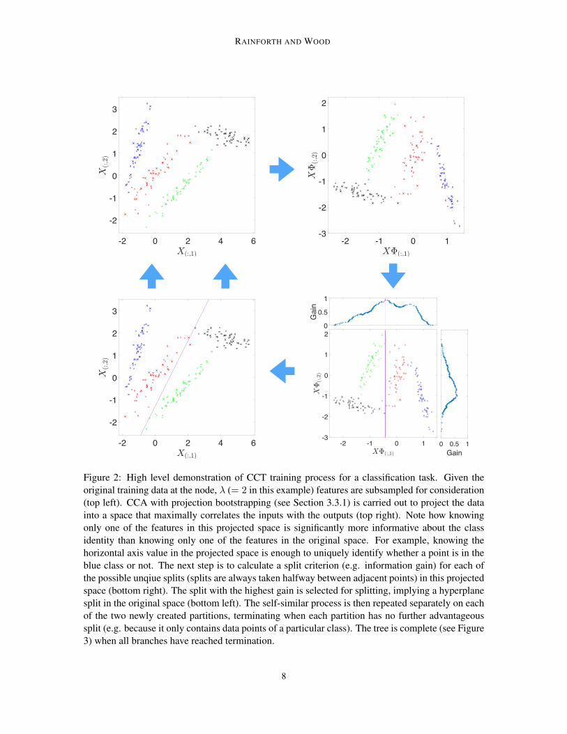
There are two key differences between the training algorithms for CCFs and RFs. Firstly, for RFtraining each tree is trained on a bootstrap sample of the data in a process known as bagging, whilefor CCFs, each tree is trained on the full training dataset. Secondly, CCFs consider a different set ofsplit candidates. In RF training then a random subset of the features are considered at each node andthe set of split candidates corresponds to all unique axis aligned partitions of the data using thesefeatures. In CCF training a random subset of the features is also taken, but CCA with projectionbootstrapping (see Section 3.3.1) is used first to project the features into canonical component space,with the set of split candidates corresponding to the unique partitions in this projected space. Thechosen partition then implies a hyperplane split that can be used directly at test time. This trainingprocess is summarized in Figure 2, using an example classification problem. The resulting CCTalong with an axis aligned alternative is shown in Figure 3.

3.2 Forest Definition and Prediction

Though CCFs are able to deal with categorical inputs, missing data, and multiple outputs (seeSections 3.3.2 and 6), we neglect these cases for now in the interest of clarity. Our aim is to makepredictions v ∈ V about outputs y ∈ Y, given corresponding vectors of input features x ∈ RD. Forregression, the outputs y are single numeric values y ∈ R. For classification, the outputs are classlabels k ∈ 1, . . . ,K, but for notational convenience we represent these using a 1-of-K encodingy ∈ IK , where for class k the kth element of y is set to 1 and all other values are set to 0. Though thepredictions convey information about the outputs, it need not be the case that V = Y. For example,for classification we consider predicting relative class probabilities, v ∈ [0, 1]K , as we are uncertainabout the true class. For regression we will only consider predicting a point estimate for the output,i.e. V = Y, though it is possible to also calculate uncertainty estimates in the same way as for RFs(see for example Criminisi et al. (2011)).

CCFs represent a supervised learning approach and so require training using labelled inputpairs. Once trained, prediction can be carried out at arbitrary input points. We consider using atraining dataset comprising of N inputs X = xnNn=1 and corresponding outputs Y = ynNn=1.Here X and Y can be conveniently represented as matrices, with the first index denoting the datapoint by convention. We use the notation X(u,v) for indexing, where u and v can both be eitherscalars or vectors of indexes and : indicates all instances in that dimension. Thus, for example,Y(1,:) corresponds to y1 andX([1,4],[2,3]) denotes a matrix containing the second and third features ofthe first and fourth data points. Vectors are indexed in the same way. For example x([1,3]) representsthe first and third dimensions (i.e. features) of x.

Let T = tii=1...L denote a CCF, comprising of L individual canonical correlation trees(CCTs) ti. When clear from the context, we will omit the tree index i to avoid clutter. As withclassical decision trees, CCTs define a hierarchical partitioning on the input space. Each individualtree ti = Ψ,Θ is defined by a set of discriminant nodes Ψ = ψjj∈J\∂J and a set of leaf nodesΘ = θjj∈∂J where J ⊂ Z≥0 is the set of node indices and ∂J ⊆ J is the subset of leaf nodeindices. Each discriminant node is defined by the tuple ψj = j, δj , φj , sj , χj,`, χj,r where j is theunique node identifier, δj ∈ 1, . . . , Dλ is a vector of indexes giving the features used for splitting

7

RAINFORTH AND WOOD

-2 -1 0 1-3

-2

-1

0

1

20

0.5

1

Gain

0 0.5 1Gain

-2 0 2 4 6

-2

-1

0

1

2

3

-2 -1 0 1-3

-2

-1

0

1

2

-2 0 2 4 6

-2

-1

0

1

2

3

Figure 2: High level demonstration of CCT training process for a classification task. Given theoriginal training data at the node, λ (= 2 in this example) features are subsampled for consideration(top left). CCA with projection bootstrapping (see Section 3.3.1) is carried out to project the datainto a space that maximally correlates the inputs with the outputs (top right). Note how knowingonly one of the features in this projected space is significantly more informative about the classidentity than knowing only one of the features in the original space. For example, knowing thehorizontal axis value in the projected space is enough to uniquely identify whether a point is in theblue class or not. The next step is to calculate a split criterion (e.g. information gain) for each ofthe possible unqiue splits (splits are always taken halfway between adjacent points) in this projectedspace (bottom right). The split with the highest gain is selected for splitting, implying a hyperplanesplit in the original space (bottom left). The self-similar process is then repeated separately on eachof the two newly created partitions, terminating when each partition has no further advantageoussplit (e.g. because it only contains data points of a particular class). The tree is complete (see Figure3) when all branches have reached termination.

8

CANONICAL CORRELATION FORESTS

-2 0 2 4 6

-2

-1

0

1

2

3

-2 0 2 4 6

-2

-1

0

1

2

3

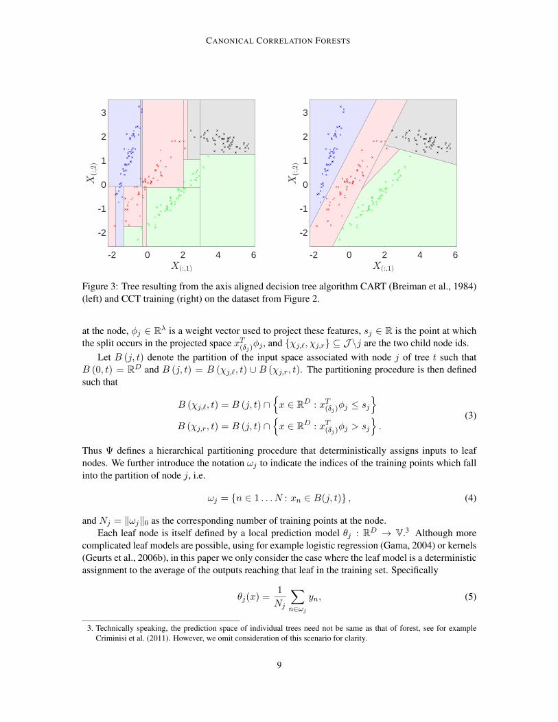
Figure 3: Tree resulting from the axis aligned decision tree algorithm CART (Breiman et al., 1984)(left) and CCT training (right) on the dataset from Figure 2.

at the node, φj ∈ Rλ is a weight vector used to project these features, sj ∈ R is the point at whichthe split occurs in the projected space xT(δj)φj , and χj,`, χj,r ⊆ J \j are the two child node ids.

Let B (j, t) denote the partition of the input space associated with node j of tree t such thatB (0, t) = RD and B (j, t) = B (χj,`, t) ∪ B (χj,r, t). The partitioning procedure is then definedsuch that

B (χj,`, t) = B (j, t) ∩x ∈ RD : xT(δj)φj ≤ sj

B (χj,r, t) = B (j, t) ∩

x ∈ RD : xT(δj)φj > sj

.

(3)

Thus Ψ defines a hierarchical partitioning procedure that deterministically assigns inputs to leafnodes. We further introduce the notation ωj to indicate the indices of the training points which fallinto the partition of node j, i.e.

ωj = n ∈ 1 . . . N : xn ∈ B(j, t) , (4)

and Nj = ‖ωj‖0 as the corresponding number of training points at the node.Each leaf node is itself defined by a local prediction model θj : RD → V.3 Although more

complicated leaf models are possible, using for example logistic regression (Gama, 2004) or kernels(Geurts et al., 2006b), in this paper we only consider the case where the leaf model is a deterministicassignment to the average of the outputs reaching that leaf in the training set. Specifically

θj(x) =1

Nj

∑n∈ωj

yn, (5)

3. Technically speaking, the prediction space of individual trees need not be same as that of forest, see for exampleCriminisi et al. (2011). However, we omit consideration of this scenario for clarity.

9

RAINFORTH AND WOOD

such that the tree’s prediction is independent of the input, given the leaf assignment. We thereforedrop the dependence on x, such that each leaf node is fully defined by its identifier j and predictionθj ∈ V.

As with RFs, out of sample prediction in CCFs is done using an equally weighted voting schemeof the tree predictions. Slightly abusing notation, let ti (x) ∈ V denote the prediction of ti for inputx. The forest’s prediction is then given by

T (x) =1

L

L∑i=1

ti (x) . (6)

We note that more complicated methods of combining the tree predictions could be used instead,see, for example, Robnik-Sikonja (2004) and (Geurts et al., 2006b).

3.3 Forest Training

Algorithms 1 and 2 give a step by step walk-through for training a CCF, outlining the forest trainingand tree growing processes respectively. In both cases some simplifications have been made forclarity, with more comprehensive algorithm blocks provided in Appendix B, additionally detailingthings such as categorical features and missing data. As we can see from Algorithm 1, CCF trainingrequires as inputs the data X,Y , a number number of trees L ∈ Z+, a number of features tosub-sample λ ∈ 1, . . . , D, an impurity measure g : YZ+ → R (see (12) and (13)), and stoppingcriteria c (see Section 3.3.3). Other than the data, all of these required inputs have default values,meaning that CCFs can be trained without parameter tuning, as is done in all of our experiments.Setting these options will be discussed in 3.3.3, for now we just note that all these options areshared with RFs and therefore the intuition for how they should be set predominantly transfers.We therefore also refer the reader to previous work that examines the effect these parameters ondecision tree ensembles more generally, e.g. Bernard et al. (2009); Criminisi et al. (2011).

As should hopefully be clear by now, each tree in a CCF is trained independently using thefull dataset. The tree training process, GROWTREE, is self similar, starting at the root node withthe full dataset. At each call it selects an optimal split for a set of generated candidates (lines 1to 18); decides whether to assign the current node as a leaf or discriminant node (line 19); and thenif the node is assigned as a decision node, it recursively calls GROWTREE again (with appropriatepartitions of the data) to produce sub-trees for each of the newly generated child nodes (lines 26to 29). The training process is complete once all generated branches have terminated as leaf nodes.

The process for deciding whether to assign a node as a leaf node or a decision node is straight-forward - the node is assigned to be a leaf if no split is beneficial (as per the split gain discussedlater) or if a stopping criterion is met (see Section 3.3.3). Otherwise it becomes a decision node.The key part of the algorithm is therefore the process for selecting the split, namely selecting thefeatures used for splitting δj , the projection vector φj , and the split point sj . This can be further bro-ken down into generating a set of candidate splits and selecting the optimal split from this candidateset.

As in RFs, the process of generating the set of candidate splits for CCFs starts by randomlysampling, δj , the subset of the features to consider at that node (lines 1 and 2 of Algorithm 2). Thiscorresponds to sampling λ features without replacement from all of those present. For RFs, the setof candidate splits comprises of all unique axis-aligned splits using these features. For CCFs thecandidate splits will be hyperplane splits implied by the possible axis-aligned splits in a projected

10

CANONICAL CORRELATION FORESTS

Algorithm 1: CCF training algorithm

Inputs: features X ∈ RN×D, outputs Y ∈ YN , number of trees L ∈ Z+ (default is 500), number offeatures to sub-sample λ ∈ 1, . . . , D (default is dlog2(D) + 1e), impurity measure g : YZ+ → R(default is (12) for classification and (13) for regression), stopping criteria c (see Section 3.3)

Outputs: CCF T1: Preprocess X . See Section 3.3.32: for i = 1: L do3: Randomly assign missing values in X . See Section 3.3.34: ti ← GROWTREE(0, X, Y, λ, g, c) . Each tree trained independently5: end for6: return T = tii=1...L

Algorithm 2: GROWTREE

Inputs: unique node identifier for root node j, Xj = X(ωj ,:) ∈ RNj×D, Y j = Y(ωj ,:) ∈ YNj , λ, g, cOutputs: subtree Ψj ,Θj where Ψj are discriminant nodes and Θj leaf nodes

1: Subsample features ids δj by sampling from 1, . . . , D λ times without replacement.2: Set X ← Xj

(:,δj)

3: Construct a bootstrap sample X ′,Y ′ by sampling Nj data points with replacement fromX , Y j

4: Φ,Ω ← CCA(X ′,Y ′) . Calculate CCA coefficients using bootstrap sample5: U ← XΦ . Project original features into canonical component space6: Gbase ← g

(Y j)

. Impurity of current node7: νmax = min (rank (X ′) , rank (Y ′)) . Number of projections8: for ν ∈ 1 : νmax do . Evaluate splits for each projection9: u← SORT(U(:,ν))

10: for i ∈ 2 : Nj do . Exhaustive search on unique splits11: S(i,ν) ← (u(i−1) + u(i))/2 . Split halfway between consecutive points12: τ ` ←

n ∈ 1, . . . , Nj : U(n,ν) ≤ S(i,ν)

. Points that would be assigned to left child

13: Nχj,` ← number of elements in τ `

14: τ r ← 1, . . . , Nj \τ `

15: G(i,ν) ← Gbase −Nχj,`Nj

g(Y(τ`,:)

)− Nj−Nχj,`

Njg(Y(τr,:)

). Split gain

16: end for17: end for18: i∗, ν∗ ← argmaxi,ν G(i,ν) . Choose best split19: if G(i∗,ν∗) ≤ 0 (i.e. no split is beneficial) or any stopping of criteria c satisfied then . Node is a leaf20: θj ← 1

Nj

∑Njn=1 Y

j(n,:) . Predictive model is average of points at leaf

21: return ·, j, θj22: else . Node is a discriminant node23: Generate unique identifiers for children χj,` and χj,r24: φj ← Φ(:,ν∗), sj ← S(i∗,ν∗) . Chosen projection and split point25: ψj ← j, δj , φj , sj , χj,`, χj,r26: τ ` ←

n ∈ 1, . . . , Nj : U(n,ν∗) ≤ S(i∗,ν∗)

. Assign data points to children

27: τ r ← 1, . . . , Nj \τ `28: Ψ`,Θ` ← GROWTREE(χj,`, X

j(τ`,:)

, Y j(τ`,:)

, λ, g, c) . Recurse for left child and right child

29: Ψr,Θr ← GROWTREE(χj,r, Xj(τr,:), Y

j(τr,:), λ, g, c)

30: return ψj ∪Ψ` ∪Ψr,Θ` ∪Θr31: end if

11

RAINFORTH AND WOOD

space XΦ. To calculate Φ, we first take a bootstrap sample of the local data at the node X ′,Y ′(line 3 of Algorithm 2). Using this bootstrap sample we then carry out a CCA between the featuresand the outputs (line 4 of Algorithm 2)

[Φ,Ω] = CCA(X ′,Y ′

)(7)

where Φ and Ω are the canonical coefficients corresponding to X ′ and Y ′ respectively. We note thatΩ is not directly used by the algorithm. Our set of candidate splits is now the unique axis-alignedsplits in the projection of the original input features into the canonical component space, namely(line 4 of Algorithm 2)

U = X(ωj ,δj)Φ (8)

remembering that ωj is the index of data points present at node j. Choosing a split in the space ofU implies a hyperplane split in the space of X , given by the projection φj , corresponding to oneof the columns of Φ, and the split point sj in the projected space. Note that CCA is only requiredduring the training phase with the splitting rule (3) used directly for out of sample prediction.

The process of choosing the best split from the set of possible candidates is analogous to theexhaustive search approach used by most decision tree methods (including RFs). The only differ-ence is that the search uses U instead of X(ωj ,δj). The core idea is to use an impurity criteriong : YZ+ → R and to choose the split which most reduces the impurity (lines 15 and 18 of Algo-rithm 2). Namely we wish to solve

φj , sj = argmaxφ∈Φ,s∈R

G(Y(ωj ,:), φ, s

)= argmax

φ∈Φ,s∈R

(g(Y(ωj ,:)

)−Nχj,`

Njg(Y(ωχj,` ,:)

)−Nχj,r

Njg(Y(ωχj,r ,:)

))(9)

where G(Y(ωj ,:), φ, s

)is commonly referred to as the gain of a split and using (3), (4), and (8) we

have that

ωχj,` (φ, s) =n ∈ ωj : X(n,δj)φ ≤ s

(10)

ωχj,r (φ, s) =n ∈ ωj : X(n,δj)φ > s

= ωj\ωχj,` (φ, s) . (11)

We see that the gain of a split depends only on how the data points are assigned to each of thechildren, such that any φ, s that leads to the same partitioning of the training data gives the samegain. By construction we already have that there are only a finite number of φ considered andso the set of unique possible splits is now fully defined by the associated values of s that leadto distinct partitions of the training data. We define this by restricting valid splits to be halfwaybetween consecutive points in the respective sorted column of U (see lines 9 and 11 of Algorithm 2).Consequently there are (Nj − 1)νmax possible splits where νmax is the number of columns of Φ(see Section 2.3).

The choice of impurity criterion depends on whether classification or regression is being per-formed. The intuitive property we desire for the impurity criterion is that it is high when the uncer-tainty in the output is high or equivalently when homogeneity in the outputs for points at the node

12

CANONICAL CORRELATION FORESTS

is low. For classification we take as a default the entropy of the node defined as

g(Y(ωj ,:)

)= −

K∑k=1

pk log2 pk (12)

where pk is the empirical probability of class k at the node, namely pk = 1Nj

∑n∈ωj Y(n,k). The

entropy impurity criterion is thus the entropy of the predictive distribution that would be generatedif the node were to become a leaf. Using the entropy as the impurity metric corresponds to usinginformation gain as the split criterion, as introduced by Quinlan (1986). A common alternativefor classification is the Gini impurity g

(Y(ωj ,:)

)= 1 −

∑Kk=1 p

2k (Breiman et al., 1984). Entropy

is taken as a default due to slightly superior performance in our experiments, but we note thatperformance variations were small and the overall improvement was certainly not definitive.

For regression we use the empirical variance,

g(Y(ωj)

)=

1

Nj

∑n∈ωj

Y 2(n) −

1

Nj

∑n∈ωj

Y(n)

2

, (13)

as an impurity measure (Breiman et al., 1984). Using this impurity measure is often referred to asthe mean squared error split criterion as it corresponds to the mean square error that would resultfrom using the mean of the samples (which is the predictive model taken if the node is a leaf)as the prediction for the training data at that node. Alternative split criteria, such those based oncurvature (Loh, 2002), could also be used, but we will not consider these further here.

Given a split and the assignment of the node to be a decision node, all that remains is to recurseto the children. This simply involves assigning all datapoints to either the left or right child using (3)(lines 26 and 27 in Algorithm 2) and calling GROWTREE for each child using the correspondingpartition of the training data.

3.3.1 PROJECTION BOOTSTRAPPING

We refer to calculating the projection matrix Φ using a local bootstrap sampling of the data but thenusing the original dataset for choosing the split in the projected space as projection bootstrapping.The motivation for projection bootstrapping, instead of say using bagging, is that it retains all theinformation from the dataset when choosing φj , sj from the candidates, thereby improving thepredictive accuracy of individual trees. This is beneficial because the use of hyperplane splits in-creases the diversity of the ensemble compared with axis-aligned forests. Therefore less artificialrandomness needs to be added to the tree training process to sufficiently decorrelate the tree predic-tions. Consequently, as shown in Section 4, projection bootstrapping leads to improved ensemblepredictive performance compared to bagging. We found, on the other hand, that omitting bothbagging and projection bootstrapping, and thus relying on random subspacing alone to decorrelatetree predictions, reduced the randomness in the tree training process too far, leading to degradedperformance.

An important exception to using projection bootstrapping is in the case where λ = D, i.e. whenwe consider all of the features at each node, for which we use bagging instead. The reason for thisis that no feature subspacing occurs in this scenario and so additional randomness needs to be addedinto the training process to prevent overfitting. Using the default settings for λ, this scenario occursonly when D ≤ 2.

13

RAINFORTH AND WOOD

3.3.2 DATA PREPROCESSING

The format of our forest definition given in Section 3.2 requires X to be in numerical form. Thisis not a problem for ordered categorical features which can simply be treated as numerical featuresusing the class index. For unordered categorical features xc ∈ S , where S represents the spaceof arbitrary qualitative attributes, we use a 1-of-K encoding such that the feature is converted intoK binary features. To ensure equal probability of selecting categorical and numerical features,the expanded binary array of each categorical feature is still treated as a single feature during therandom subspacing (i.e. sampling δj , see Algorithm 5). In the rest of the paper we refer to numeric,binary, and ordered categorical features (i.e. those that do not require this expansion) as ordinal andnon-ordered categorical features as non-ordinal.

A second preprocessing step is to centre and rescale the input data so that it has zero mean andunit variance for each dimension (ignoring any missing data). As CCA and the split criteria areinvariant under affine transformations of the full dataset, this does not have any direct bearing onthe tree training. However it ensures equal influence of the input features in the rank reduction usedto ensure stability of the CCA calculation as described in Section A.

The final preprocessing step is to deal with missing data. Here we take the simple approachof randomly assigning each missing value in X to a random draw from a unit Gaussian (notingthat we have previously ensure that each feature has zero mean and unit variance). This is doneindependently for each tree so that each tree is affected in a different way. The same approach isused for both training and testing. Though we found this simple approach worked well in practise,one could also envisage using more complicated schemes, such as sampling from the empiricaldistribution of the feature over the training data instead.

3.3.3 STOPPING CRITERIA AND OTHER PARAMETER SETTINGS

As previously stated, the CCF training algorithm has four parameters of note: the number of treesL, the number of features to sub-sample at each node λ, the impurity measure g, and the stoppingcriteria c. We reiterate that all of these parameters are common to RFs.

Setting g has already been discussed in Section 3.3, using entropy and variance as defaults forclassification and regression respectively. The setting of L need only be based on computationalbudget as it is commonly accepted (Criminisi et al., 2011), and there are theoretical results sug-gesting (Breiman, 2001; Biau, 2012), that more trees is always preferable for common decisionensemble methods (with the exception of boosting which can overfit if L is too large). We takeL = 500 as a default value as compromise between speed and accuracy, noting that, as shown inSection 7.4, the misclassification rate has usually stabilized by this value of L. It may often, how-ever, be beneficial to use significantly smaller values for L when speed is paramount none-the-less.From this perspective CCFs offer the potential for significant speed improvements over RFs, as wefound that on average only 15 CCTs are required to match the accuracy of 500 RF trees (see Sec-tion 7.4). When the number of features is very large, it may also be beneficial to use more than 500trees.

The default number of features to sample at each step is taken to be λ = dlog2 (D) + 1e whered·e represents the ceiling function, with the exception that we set λ = 2 whenD = 3 so that randomsubspacing and CCA can both be employed. This is the default setting taken by, for example, theWEKA RF implementation (Hall et al., 2009). It has the advantage of being very fast, as the trainingcost subsequently scales logarithmically with the number of features (see Section 7.2). We also

14

CANONICAL CORRELATION FORESTS

found that it was also an effective choice in terms of empirical predictive accuracy, outperformingthe other common choice of λ =

⌈√D⌉

. One could of course also tune λ at the expense of trainingspeed, but we note that results in the recent survey of Fernandez-Delgado et al. (2014), along weour own comparisons to their results, suggest that there is no noticeable difference between theperformance of RF packages that tune hyperparameters and those that do not. We further refer thereader to the study for the effect of λ on RF performance by Bernard et al. (2009).

Though a number of possible stopping criteria exist (Criminisi et al., 2011), the main two usedin practice are a maximum tree depth, beyond which all nodes are assigned as leaves (our defaultis ∞), and a minimum number of contained datapoints for which a node is allowed to split (ourdefault is 2 for classification and 6 for regression). Though not technically a stopping criterion, acommon associated parameter (omitted from the algorithm blocks) is a minimum number of data-points allowed for a generated leaf node (our default is 1 for classification and 3 for regression). Assuch, only splits that assign at least this many points to a leaf are considered. The rational for thesestopping criteria is to try and guard against potential overfitting, particularly when the L is small.Our default settings are again in line with the defaults of the WEKA RF implementation (Hall et al.,2009). We note that the default settings for classification correspond to using no stopping criteria(other than assigning the node to be a leaf when no split is beneficial). The default settings forregression are slightly more conservative, reflecting a greater apparent tendency for decision treeensembles to overfit for regression problems then classification problems. However, it may that thisapparent tendency is due more to the error metrics that are typically used for assessing the two (i.e.mean squared error compared to misclassification rate), rather than any inherent tendencies of thealgorithms themselves.

4. Classification Experiments

4.1 Comparison to State-of-the-art Tree Ensembles

To investigate the predictive performance of CCFs, we ran comparison tests against RFs and rotationforest (Rot-For) over a broad variety of datasets. The results show that CCFs significantly outper-formed both methods and create a new benchmark in classification accuracy for out-of-the-boxdecision tree ensembles, despite being a considerably more computationally efficient than rotationforests as discussed in Section 7.2.

To better understand the key factors behind these improvements, we also considered a numberof variations of the CCF algorithm. Firstly, we considered using bagging, as per RF, instead ofprojection bootstrapping. We refer to this algorithm as CCF-Bag.

Secondly, we considered the effect of uniformly sampling the projection matrix, Φ, from thespace of valid rotation matrices, instead of using CCA. Here our notion of a uniform distributionover rotations is based on the Haar measure as discussed by Diaconis and Shahshahani (1987) andBlaser and Fryzlewicz (2016). We refer to this approach as random rotation forests (RRFs). Tocarry out the required rotation matrix sampling, RRFs use the procedure laid out in Blaser andFryzlewicz (2016) based on a QR decomposition (Householder, 1958) of independent draws froma unit Gaussian. Note that, unlike Blaser and Fryzlewicz (2016), the random rotation in RRFs iscarried out at separately each node, as opposed to using a single rotation for the whole tree.

Finally we considered using RRFs with the addition of bagging, referring to this as algorithmas RRF-Bag. RRF-Bag shares similarity with the Forest-RC algorithm of Breiman (2001). A key

15

RAINFORTH AND WOOD

difference is that Forest-RC independently samples elements of the projection matrix uniformly inthe range −1,+1, biasing the projected features, U = XΦ, away from the original axis com-pared with uniformly sampling rotations. Forest-RC also allows sparsity by calculating np separateprojections, each with a maximum of nv non-zero values, such that Φ is constructed as a D × npmatrix where there are only nv values are nonzero in each column. We do not consider Forest-RCdirectly here, but note that previous results suggest that its average performance is similar to RFs.

MATLAB’s TreeBagger function was used for the RF implementation, while our own MAT-LAB implementation4 was used for CCFs, CCF-Bag, RRFs, and RRF-Bag. As per the defaultparameters given in 3.3.3, each ensemble was built using L = 500 trees, λ = dlog2 (D) + 1e (withthe exception λ = 2 when D = 3), the entropy impurity criterion, and no stopping criteria otherthan stopping when no split is beneficial. The choice of the entropy impurity criterion over the Giniimpurity criterion and setting λ = dlog2 (D) + 1e rather than the common alternative λ =

⌈√D⌉

was made on the basis that both choices gave improved predictive performance for RFs on averagecompared with these alternatives. For CCFs, CCF-Bag, RRFs and RRF-Bag, missing values weresampled randomly for each tree as explain in 3.3.2 while for RFs they were dealt with internally bythe TreeBagger function.

Rotation Forests were implemented in WEKA (Hall et al., 2009) with 500 trees and the defaulttree options except that we used binary, unpruned, trees and set the minimum number of instancesper leaf to 1. In addition to keeping the implementation of rotation forest as consistent as possiblewith the other algorithms, these settings dominated rotation forests of the same size with the defaultoptions over a single cross validation. As recommended by Rodriguez et al (Rodriguez et al., 2006),1-of-K encoding was used for non-ordinal features for rotation forests (note rotation forests do notthen treat them differently to ordinal variables), while missing values were replaced by the mean.

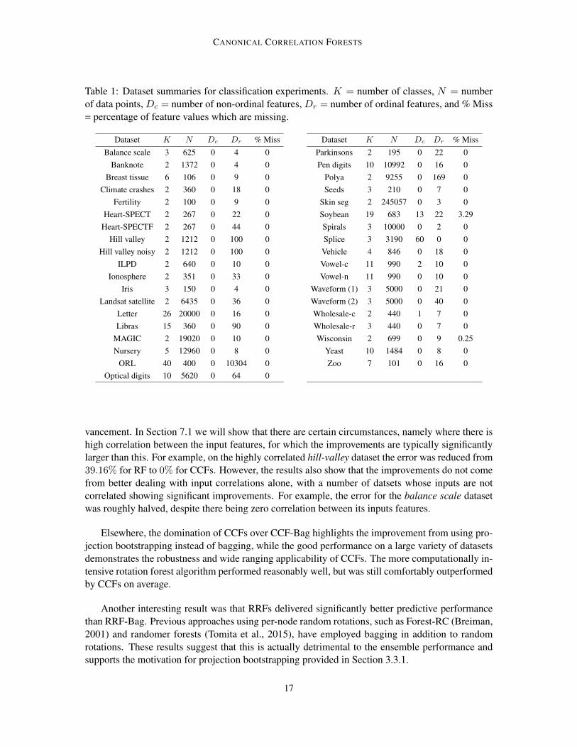
The majority of the 37 datasets considered were taken from the UCI machine learning database5

(Lichman, 2013) with the exceptions of the ORL face recognition dataset (Samaria and Harter,1994), the Polyadenylation Signal Prediction (polya) dataset (Li and Liu, 2002), and the artificialspiral dataset from Figure 1. Summaries of the datasets are given in Table 1. Note for the vowel-cdataset the sex and identifier for the speaker are included, whereas these are omitted for the vowel-n dataset which is otherwise identical. The wholesale-c and wholesale-r datasets correspond topredicting the channel and region attributes respectively.

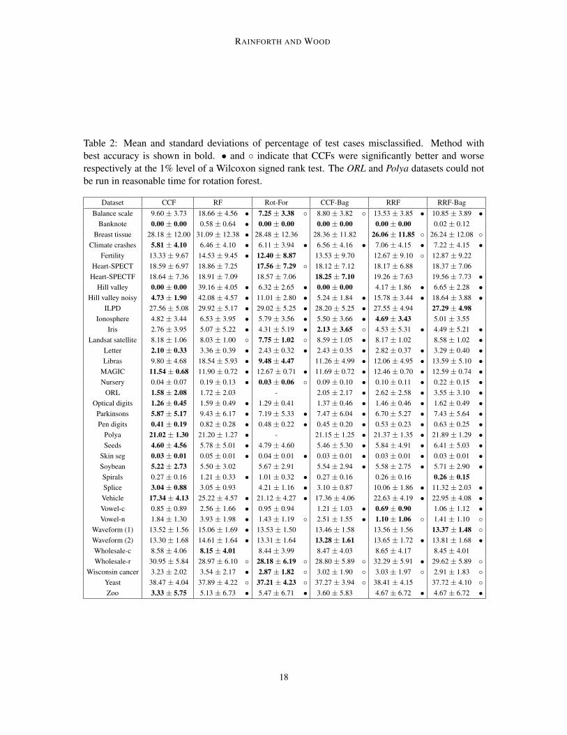
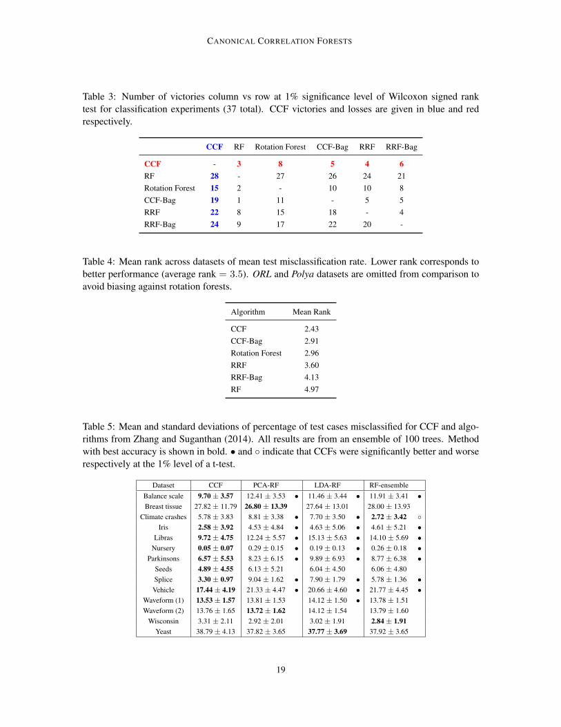
For each dataset, 15 different 10-fold cross-validation tests were performed, results from whichare given in Table 2. Table 3 shows a summary of results over all the datasets, giving the num-ber of datasets for which the performance of one dataset was significantly better than another atthe 1% level of a Wilcoxon signed rank test. Table 4 shows the average performance ranks of thealgorithms. These results show that CCFs performed excellently, comfortably outperforming allthe other approaches. The improvement compared to RFs was particularly large, with RFs havingon average 1.74 times as many misclassifications as CCFs (ignoring the two datasets where CCFshad perfect accuracy). To give another perspective, if one were using RFs and decided to switchto CCFs, then the number of misclassifications would be reduced by a factor of 28.7% on aver-age for the tested datasets. We emphasise that these are improvements over a generic selection ofdatasets, rather than being carefully chosen problems. Therefore the magnitude and regularity (33of 37 datasets had lower error for CCFs than RFs) of the improvements represents a substantial ad-

4. https://github.com/twgr/ccfs/5. https://archive.ics.uci.edu/ml/datasets.html

16

CANONICAL CORRELATION FORESTS

Table 1: Dataset summaries for classification experiments. K = number of classes, N = numberof data points, Dc = number of non-ordinal features, Dr = number of ordinal features, and % Miss= percentage of feature values which are missing.

Dataset K N Dc Dr % Miss

Balance scale 3 625 0 4 0Banknote 2 1372 0 4 0

Breast tissue 6 106 0 9 0Climate crashes 2 360 0 18 0

Fertility 2 100 0 9 0Heart-SPECT 2 267 0 22 0

Heart-SPECTF 2 267 0 44 0Hill valley 2 1212 0 100 0

Hill valley noisy 2 1212 0 100 0ILPD 2 640 0 10 0

Ionosphere 2 351 0 33 0Iris 3 150 0 4 0

Landsat satellite 2 6435 0 36 0Letter 26 20000 0 16 0Libras 15 360 0 90 0

MAGIC 2 19020 0 10 0Nursery 5 12960 0 8 0

ORL 40 400 0 10304 0Optical digits 10 5620 0 64 0

Dataset K N Dc Dr % Miss

Parkinsons 2 195 0 22 0Pen digits 10 10992 0 16 0

Polya 2 9255 0 169 0Seeds 3 210 0 7 0

Skin seg 2 245057 0 3 0Soybean 19 683 13 22 3.29Spirals 3 10000 0 2 0Splice 3 3190 60 0 0Vehicle 4 846 0 18 0Vowel-c 11 990 2 10 0Vowel-n 11 990 0 10 0

Waveform (1) 3 5000 0 21 0Waveform (2) 3 5000 0 40 0Wholesale-c 2 440 1 7 0Wholesale-r 3 440 0 7 0Wisconsin 2 699 0 9 0.25

Yeast 10 1484 0 8 0Zoo 7 101 0 16 0

vancement. In Section 7.1 we will show that there are certain circumstances, namely where there ishigh correlation between the input features, for which the improvements are typically significantlylarger than this. For example, on the highly correlated hill-valley dataset the error was reduced from39.16% for RF to 0% for CCFs. However, the results also show that the improvements do not comefrom better dealing with input correlations alone, with a number of datsets whose inputs are notcorrelated showing significant improvements. For example, the error for the balance scale datasetwas roughly halved, despite there being zero correlation between its inputs features.

Elsewhere, the domination of CCFs over CCF-Bag highlights the improvement from using pro-jection bootstrapping instead of bagging, while the good performance on a large variety of datasetsdemonstrates the robustness and wide ranging applicability of CCFs. The more computationally in-tensive rotation forest algorithm performed reasonably well, but was still comfortably outperformedby CCFs on average.

Another interesting result was that RRFs delivered significantly better predictive performancethan RRF-Bag. Previous approaches using per-node random rotations, such as Forest-RC (Breiman,2001) and randomer forests (Tomita et al., 2015), have employed bagging in addition to randomrotations. These results suggest that this is actually detrimental to the ensemble performance andsupports the motivation for projection bootstrapping provided in Section 3.3.1.

17

RAINFORTH AND WOOD

Table 2: Mean and standard deviations of percentage of test cases misclassified. Method withbest accuracy is shown in bold. • and indicate that CCFs were significantly better and worserespectively at the 1% level of a Wilcoxon signed rank test. The ORL and Polya datasets could notbe run in reasonable time for rotation forest.

Dataset CCF RF Rot-For CCF-Bag RRF RRF-BagBalance scale 9.60 ± 3.73 18.66 ± 4.56 • 7.25 ± 3.38 8.80 ± 3.82 13.53 ± 3.85 • 10.85 ± 3.89 •

Banknote 0.00 ± 0.00 0.58 ± 0.64 • 0.00 ± 0.00 0.00 ± 0.00 0.00 ± 0.00 0.02 ± 0.12Breast tissue 28.18 ± 12.00 31.09 ± 12.38 • 28.48 ± 12.36 28.36 ± 11.82 26.06 ± 11.85 26.24 ± 12.08

Climate crashes 5.81 ± 4.10 6.46 ± 4.10 • 6.11 ± 3.94 • 6.56 ± 4.16 • 7.06 ± 4.15 • 7.22 ± 4.15 •Fertility 13.33 ± 9.67 14.53 ± 9.45 • 12.40 ± 8.87 13.53 ± 9.70 12.67 ± 9.10 12.87 ± 9.22

Heart-SPECT 18.59 ± 6.97 18.86 ± 7.25 17.56 ± 7.29 18.12 ± 7.12 18.17 ± 6.88 18.37 ± 7.06Heart-SPECTF 18.64 ± 7.36 18.91 ± 7.09 18.57 ± 7.06 18.25 ± 7.10 19.26 ± 7.63 19.56 ± 7.73 •

Hill valley 0.00 ± 0.00 39.16 ± 4.05 • 6.32 ± 2.65 • 0.00 ± 0.00 4.17 ± 1.86 • 6.65 ± 2.28 •Hill valley noisy 4.73 ± 1.90 42.08 ± 4.57 • 11.01 ± 2.80 • 5.24 ± 1.84 • 15.78 ± 3.44 • 18.64 ± 3.88 •

ILPD 27.56 ± 5.08 29.92 ± 5.17 • 29.02 ± 5.25 • 28.20 ± 5.25 • 27.55 ± 4.94 27.29 ± 4.98Ionosphere 4.82 ± 3.44 6.53 ± 3.95 • 5.79 ± 3.56 • 5.50 ± 3.66 • 4.69 ± 3.43 5.01 ± 3.55

Iris 2.76 ± 3.95 5.07 ± 5.22 • 4.31 ± 5.19 • 2.13 ± 3.65 4.53 ± 5.31 • 4.49 ± 5.21 •Landsat satellite 8.18 ± 1.06 8.03 ± 1.00 7.75 ± 1.02 8.59 ± 1.05 • 8.17 ± 1.02 8.58 ± 1.02 •

Letter 2.10 ± 0.33 3.36 ± 0.39 • 2.43 ± 0.32 • 2.43 ± 0.35 • 2.82 ± 0.37 • 3.29 ± 0.40 •Libras 9.80 ± 4.68 18.54 ± 5.93 • 9.48 ± 4.47 11.26 ± 4.99 • 12.06 ± 4.95 • 13.59 ± 5.10 •

MAGIC 11.54 ± 0.68 11.90 ± 0.72 • 12.67 ± 0.71 • 11.69 ± 0.72 • 12.46 ± 0.70 • 12.59 ± 0.74 •Nursery 0.04 ± 0.07 0.19 ± 0.13 • 0.03 ± 0.06 0.09 ± 0.10 • 0.10 ± 0.11 • 0.22 ± 0.15 •

ORL 1.58 ± 2.08 1.72 ± 2.03 - 2.05 ± 2.17 • 2.62 ± 2.58 • 3.55 ± 3.10 •Optical digits 1.26 ± 0.45 1.59 ± 0.49 • 1.29 ± 0.41 1.37 ± 0.46 • 1.46 ± 0.46 • 1.62 ± 0.49 •

Parkinsons 5.87 ± 5.17 9.43 ± 6.17 • 7.19 ± 5.33 • 7.47 ± 6.04 • 6.70 ± 5.27 • 7.43 ± 5.64 •Pen digits 0.41 ± 0.19 0.82 ± 0.28 • 0.48 ± 0.22 • 0.45 ± 0.20 • 0.53 ± 0.23 • 0.63 ± 0.25 •

Polya 21.02 ± 1.30 21.20 ± 1.27 • - 21.15 ± 1.25 • 21.37 ± 1.35 • 21.89 ± 1.29 •Seeds 4.60 ± 4.56 5.78 ± 5.01 • 4.79 ± 4.60 5.46 ± 5.30 • 5.84 ± 4.91 • 6.41 ± 5.03 •

Skin seg 0.03 ± 0.01 0.05 ± 0.01 • 0.04 ± 0.01 • 0.03 ± 0.01 • 0.03 ± 0.01 • 0.03 ± 0.01 •Soybean 5.22 ± 2.73 5.50 ± 3.02 5.67 ± 2.91 5.54 ± 2.94 • 5.58 ± 2.75 • 5.71 ± 2.90 •Spirals 0.27 ± 0.16 1.21 ± 0.33 • 1.01 ± 0.32 • 0.27 ± 0.16 0.26 ± 0.16 0.26 ± 0.15Splice 3.04 ± 0.88 3.05 ± 0.93 4.21 ± 1.16 • 3.10 ± 0.87 10.06 ± 1.86 • 11.32 ± 2.03 •Vehicle 17.34 ± 4.13 25.22 ± 4.57 • 21.12 ± 4.27 • 17.36 ± 4.06 22.63 ± 4.19 • 22.95 ± 4.08 •Vowel-c 0.85 ± 0.89 2.56 ± 1.66 • 0.95 ± 0.94 1.21 ± 1.03 • 0.69 ± 0.90 1.06 ± 1.12 •Vowel-n 1.84 ± 1.30 3.93 ± 1.98 • 1.43 ± 1.19 2.51 ± 1.55 • 1.10 ± 1.06 1.41 ± 1.10

Waveform (1) 13.52 ± 1.56 15.06 ± 1.69 • 13.53 ± 1.50 13.46 ± 1.58 13.56 ± 1.56 13.37 ± 1.48 Waveform (2) 13.30 ± 1.68 14.61 ± 1.64 • 13.31 ± 1.64 13.28 ± 1.61 13.65 ± 1.72 • 13.81 ± 1.68 •Wholesale-c 8.58 ± 4.06 8.15 ± 4.01 8.44 ± 3.99 8.47 ± 4.03 8.65 ± 4.17 8.45 ± 4.01Wholesale-r 30.95 ± 5.84 28.97 ± 6.10 28.18 ± 6.19 28.80 ± 5.89 32.29 ± 5.91 • 29.62 ± 5.89

Wisconsin cancer 3.23 ± 2.02 3.54 ± 2.17 • 2.87 ± 1.82 3.02 ± 1.90 3.03 ± 1.97 2.91 ± 1.83 Yeast 38.47 ± 4.04 37.89 ± 4.22 37.21 ± 4.23 37.27 ± 3.94 38.41 ± 4.15 37.72 ± 4.10 Zoo 3.33 ± 5.75 5.13 ± 6.73 • 5.47 ± 6.71 • 3.60 ± 5.83 4.67 ± 6.72 • 4.67 ± 6.72 •

18

CANONICAL CORRELATION FORESTS

Table 3: Number of victories column vs row at 1% significance level of Wilcoxon signed ranktest for classification experiments (37 total). CCF victories and losses are given in blue and redrespectively.

CCF RF Rotation Forest CCF-Bag RRF RRF-Bag

CCF - 3 8 5 4 6RF 28 - 27 26 24 21Rotation Forest 15 2 - 10 10 8CCF-Bag 19 1 11 - 5 5RRF 22 8 15 18 - 4RRF-Bag 24 9 17 22 20 -

Table 4: Mean rank across datasets of mean test misclassification rate. Lower rank corresponds tobetter performance (average rank = 3.5). ORL and Polya datasets are omitted from comparison toavoid biasing against rotation forests.

Algorithm Mean Rank

CCF 2.43CCF-Bag 2.91Rotation Forest 2.96RRF 3.60RRF-Bag 4.13RF 4.97

Table 5: Mean and standard deviations of percentage of test cases misclassified for CCF and algo-rithms from Zhang and Suganthan (2014). All results are from an ensemble of 100 trees. Methodwith best accuracy is shown in bold. • and indicate that CCFs were significantly better and worserespectively at the 1% level of a t-test.

Dataset CCF PCA-RF LDA-RF RF-ensembleBalance scale 9.70 ± 3.57 12.41 ± 3.53 • 11.46 ± 3.44 • 11.91 ± 3.41 •Breast tissue 27.82 ± 11.79 26.80 ± 13.39 27.64 ± 13.01 28.00 ± 13.93

Climate crashes 5.78 ± 3.83 8.81 ± 3.38 • 7.70 ± 3.50 • 2.72 ± 3.42 Iris 2.58 ± 3.92 4.53 ± 4.84 • 4.63 ± 5.06 • 4.61 ± 5.21 •

Libras 9.72 ± 4.75 12.24 ± 5.57 • 15.13 ± 5.63 • 14.10 ± 5.69 •Nursery 0.05 ± 0.07 0.29 ± 0.15 • 0.19 ± 0.13 • 0.26 ± 0.18 •

Parkinsons 6.57 ± 5.53 8.23 ± 6.15 • 9.89 ± 6.93 • 8.77 ± 6.38 •Seeds 4.89 ± 4.55 6.13 ± 5.21 6.04 ± 4.50 6.06 ± 4.80Splice 3.30 ± 0.97 9.04 ± 1.62 • 7.90 ± 1.79 • 5.78 ± 1.36 •Vehicle 17.44 ± 4.19 21.33 ± 4.47 • 20.66 ± 4.60 • 21.77 ± 4.45 •

Waveform (1) 13.53 ± 1.57 13.81 ± 1.53 14.12 ± 1.50 • 13.78 ± 1.51Waveform (2) 13.76 ± 1.65 13.72 ± 1.62 14.12 ± 1.54 13.79 ± 1.60

Wisconsin 3.31 ± 2.11 2.92 ± 2.01 3.02 ± 1.91 2.84 ± 1.91Yeast 38.79 ± 4.13 37.82 ± 3.65 37.77 ± 3.69 37.92 ± 3.65

19

RAINFORTH AND WOOD

4.1.1 COMPARISON TO RANDOM FORESTS WITH ENSEMBLE OF FEATURE SPACES

We next make comparisons to the PCA-RF, LDA-RF, and RF-ensemble methods introduced byZhang and Suganthan (2014). As Zhang and Suganthan (2014) performed the same cross validationtests on 14 of the common datasets, we make direct comparisons to their quoted results. Taking thefirst 100 trees from our experiments to match the ensemble sizes gives the comparisons provided inTable 5. We see that CCFs consistently outperform all three methods, giving win/draw/loss ratios atthe 1% significance level of a t-test for CCFs of 8/6/0, 9/5/0, and 7/6/1 compared to PCA-RF, LDA-RF and RF-ensemble respectively. On average PCA-RF, LDA-RF, and RF-ensemble had 1.66, 1.51and 1.49 times as many misclassifications as CCFs respectively. We reiterate that, other than PCA-RF, these methods do not extend to the regression and multiple output cases like CCFs and the otherapproaches we consider do.

4.2 Comparison to Other Classifiers

In order to provide comparison to a wider array of classifiers, we also tested CCFs using the exper-imental setup of Fernandez-Delgado et al. (2014) from their recent survey of 179 classifiers appliedto 121 datasets. We used the same partitions which were a mix of 4-fold cross validations andpredefined train / test splits.6 We omitted datasets containing non-ordinal features on the basis thatthey pre-processed such features by treating the category indexes as numeric features, which is sub-stantially different to our recommended procedure (see Section 3.3.2). For consistency with theirapproach, we fixed the missing features values (to the feature mean), rather than using the procedurelaid out in Section 3.3.2. As a check that tests were run correctly, we also ran MATLAB’s TreeBaggeralgorithm, with 500 trees and λ = dlog2 (D) + 1e, which as expected gave performance on par withthe very similar rforest R algorithm. An exception to this was the image-segmentation dataset forwhich we were unable to replicate the rforest R results to within any plausible level of variability.We therefore omitted this dataset from the results. In total 82 datasets were compared, for whichsummaries along with detailed results are available in Appendix E, while a summary of the resultsfor the top 20 performing classifiers (based on average accuracy rank) is given in Table 6. We notethat our quoted results for the competing methods differs from those of the original paper due tousing only a subset of the original datasets (averages were reprocessed using the individual datasetscores provided by Fernandez-Delgado et al. (2014)). We also note that the relatively poor perfor-mance of rotation forests that is quoted most likely stems from the fact that they set L = 10 forrotation forests and L = 500 for most of the RF implementations, constituting an arguably unfaircomparison.

Whereas Fernandez-Delgado et al. (2014) included an, often intensive, parameter tuning stepin their tests, we used CCFs in an out-of-the-box fashion, taking the same parameters as in Sec-tion 3.3.3. Despite this, CCFs outperformed all other tested classifiers based on every calculatedperformance metric. This superior performance is particularly impressive in light of the observationby Wainberg et al. (2016) that the method Fernandez-Delgado et al. (2014) use for the parametertuning positively biases the estimated predictive accuracy and κ score (Carletta, 1996) (an thus neg-atively biases the error). Namely, their parameter tuning step makes use of the full dataset (train

6. Partitions and results from Fernandez-Delgado et al. (2014) are available athttp://persoal.citius.usc.es/manuel.fernandez.delgado/papers/jmlr/

7. Note that these are not the number significant victories / losses as quoted elsewhere due to the small number of foldsconsidered.

20

CANONICAL CORRELATION FORESTS

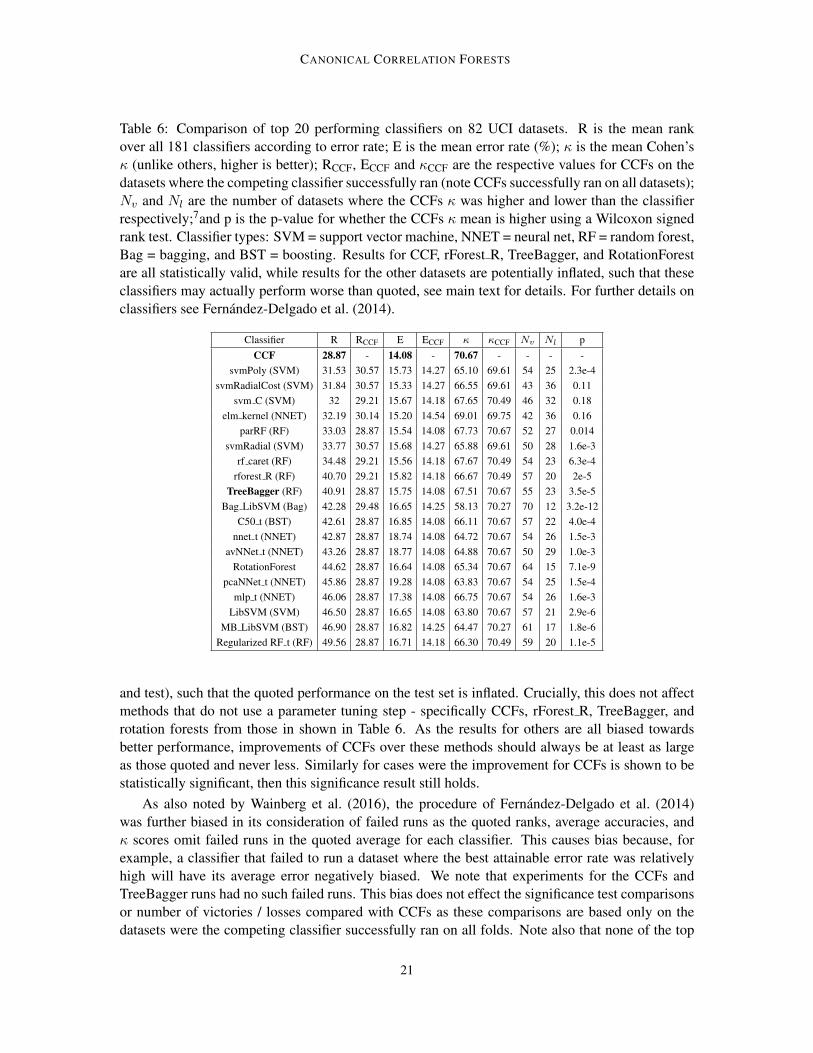
Table 6: Comparison of top 20 performing classifiers on 82 UCI datasets. R is the mean rankover all 181 classifiers according to error rate; E is the mean error rate (%); κ is the mean Cohen’sκ (unlike others, higher is better); RCCF, ECCF and κCCF are the respective values for CCFs on thedatasets where the competing classifier successfully ran (note CCFs successfully ran on all datasets);Nv and Nl are the number of datasets where the CCFs κ was higher and lower than the classifierrespectively;7and p is the p-value for whether the CCFs κ mean is higher using a Wilcoxon signedrank test. Classifier types: SVM = support vector machine, NNET = neural net, RF = random forest,Bag = bagging, and BST = boosting. Results for CCF, rForest R, TreeBagger, and RotationForestare all statistically valid, while results for the other datasets are potentially inflated, such that theseclassifiers may actually perform worse than quoted, see main text for details. For further details onclassifiers see Fernandez-Delgado et al. (2014).

Classifier R RCCF E ECCF κ κCCF Nv Nl pCCF 28.87 - 14.08 - 70.67 - - - -

svmPoly (SVM) 31.53 30.57 15.73 14.27 65.10 69.61 54 25 2.3e-4svmRadialCost (SVM) 31.84 30.57 15.33 14.27 66.55 69.61 43 36 0.11

svm C (SVM) 32 29.21 15.67 14.18 67.65 70.49 46 32 0.18elm kernel (NNET) 32.19 30.14 15.20 14.54 69.01 69.75 42 36 0.16

parRF (RF) 33.03 28.87 15.54 14.08 67.73 70.67 52 27 0.014svmRadial (SVM) 33.77 30.57 15.68 14.27 65.88 69.61 50 28 1.6e-3

rf caret (RF) 34.48 29.21 15.56 14.18 67.67 70.49 54 23 6.3e-4rforest R (RF) 40.70 29.21 15.82 14.18 66.67 70.49 57 20 2e-5

TreeBagger (RF) 40.91 28.87 15.75 14.08 67.51 70.67 55 23 3.5e-5Bag LibSVM (Bag) 42.28 29.48 16.65 14.25 58.13 70.27 70 12 3.2e-12

C50 t (BST) 42.61 28.87 16.85 14.08 66.11 70.67 57 22 4.0e-4nnet t (NNET) 42.87 28.87 18.74 14.08 64.72 70.67 54 26 1.5e-3

avNNet t (NNET) 43.26 28.87 18.77 14.08 64.88 70.67 50 29 1.0e-3RotationForest 44.62 28.87 16.64 14.08 65.34 70.67 64 15 7.1e-9

pcaNNet t (NNET) 45.86 28.87 19.28 14.08 63.83 70.67 54 25 1.5e-4mlp t (NNET) 46.06 28.87 17.38 14.08 66.75 70.67 54 26 1.6e-3

LibSVM (SVM) 46.50 28.87 16.65 14.08 63.80 70.67 57 21 2.9e-6MB LibSVM (BST) 46.90 28.87 16.82 14.25 64.47 70.27 61 17 1.8e-6

Regularized RF t (RF) 49.56 28.87 16.71 14.18 66.30 70.49 59 20 1.1e-5

and test), such that the quoted performance on the test set is inflated. Crucially, this does not affectmethods that do not use a parameter tuning step - specifically CCFs, rForest R, TreeBagger, androtation forests from those in shown in Table 6. As the results for others are all biased towardsbetter performance, improvements of CCFs over these methods should always be at least as largeas those quoted and never less. Similarly for cases were the improvement for CCFs is shown to bestatistically significant, then this significance result still holds.

As also noted by Wainberg et al. (2016), the procedure of Fernandez-Delgado et al. (2014)was further biased in its consideration of failed runs as the quoted ranks, average accuracies, andκ scores omit failed runs in the quoted average for each classifier. This causes bias because, forexample, a classifier that failed to run a dataset where the best attainable error rate was relativelyhigh will have its average error negatively biased. We note that experiments for the CCFs andTreeBagger runs had no such failed runs. This bias does not effect the significance test comparisonsor number of victories / losses compared with CCFs as these comparisons are based only on thedatasets were the competing classifier successfully ran on all folds. Note also that none of the top

21

RAINFORTH AND WOOD

20 classifiers had more than 4 failures so the effects of failed runs was relatively small. However,in the interest of correctly comparing the mean rank, mean error, and mean κ between CCFs andthe alternatives, we also provide the average metrics for CCFs on the subset of datasets whereeach classifier successfully run (see Table 6). These show that CCFs outperformed all of the otherclassifiers on all three metrics. Similarly, we found that for each classifier, the number of timesCCFs outperformed that classifier was larger than the number of times it performed worse.

5. Regression Experiments

We now investigate the predictive performance of CCFs for regression. We start with an illustrativeexample to show the benefits of CCFs over axis aligned approaches. Namely, we consider the sixhump camel function (Molga and Smutnicki, 2005)

f(x1, x2) =

(4− 2.1x2

2 +x4

2

3

)x2

2 + x1x2 + (−4 + 4x21)x2

1 (14)

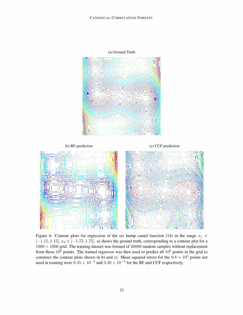
in the range x1 ∈ [−1.15, 1.15], x2 ∈ [−1.75, 1.75]. Figure 4 shows the contour plots resultingfrom training a CCF and RF on a random sample of points in this range. These show that the RFpredictions fail to catch the true contours of the function, with the RF contours noticeably alignedwith the axis to the detriment of the regressor. The CCF on the other hand is able to accuratelycapture the regression surface.

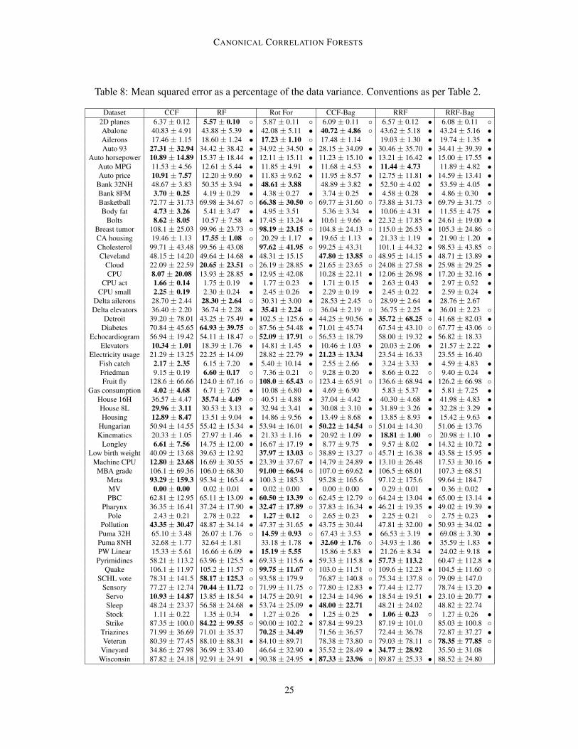
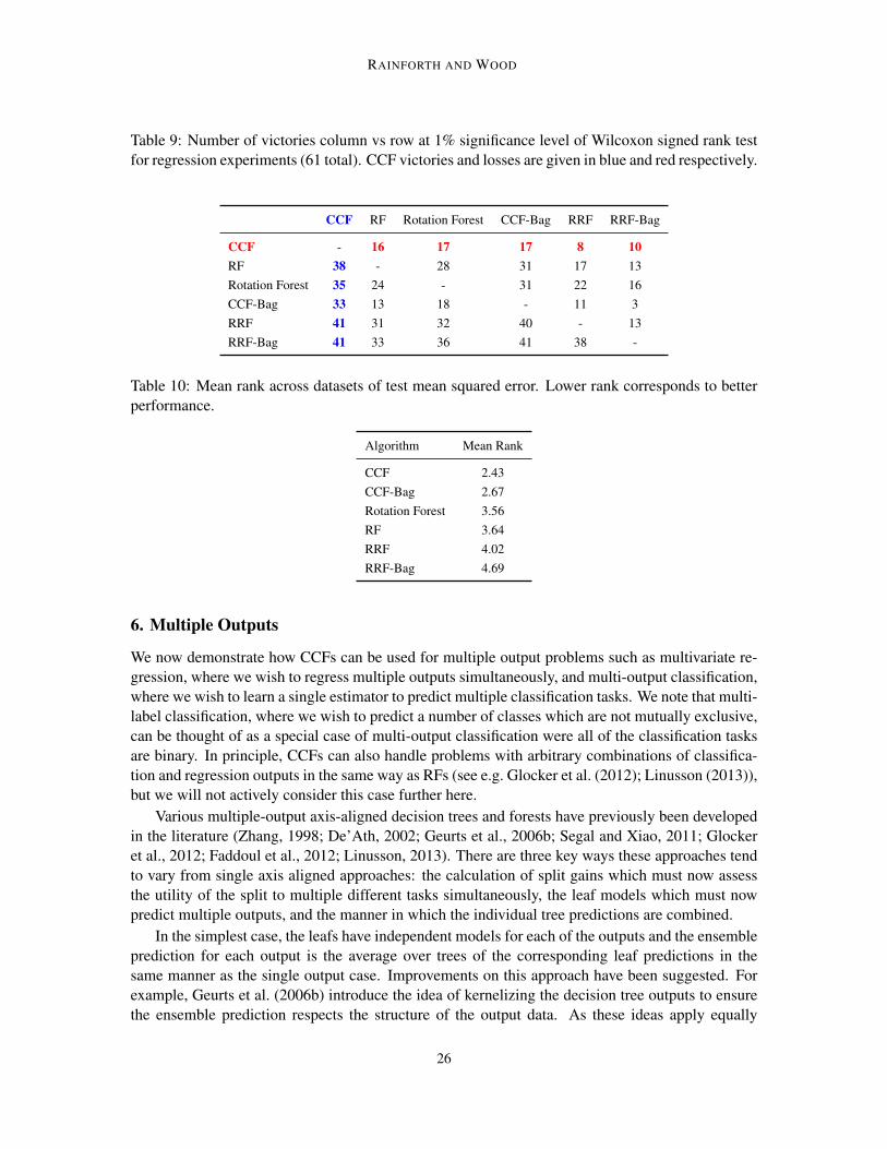
We next consider a more rigorous comparison of CCFs to RFs, rotation forests, CCF-Bag, RRFs,and RRF-bag. Parameters were again set as per Section 3.3.3, meaning that we used the meansquared error criterion and set the minimum number of points at a leaf node to 3 for all methods.All other parameters and the test procedure (i.e. 15 separate 10−fold cross-validation tests) were asper the classification experiments in Section 4.1. As in Pardo et al. (2013), we used the 61 regressiondatasets from the WEKA dataset collection8 (Hall et al., 2009), 30 of which were assembled by LuisTorgo.9 Summary information about each dataset is provided in Table 7, the full results are givenin Table 8, summaries for the significance test results are shown in Table 9, and the mean ranks aregiven in Table 10.

These results show that, as with the classification experiments, CCFs outperformed all the othermethods. Interestingly, the performance of RFs was noticeably improved relative to the other ap-proaches. Though still comfortably outperformed by CCFs and CCF-Bag, RFs performed similarlyto rotation forests and substantially better than the random rotation approaches for these problems.These results were confirmed by repeating the RF tests using the same code base as for CCFs, pro-ducing very similar results (this check was also performed for the classification experiments). Onepossible reason for this difference is that it stems from differences in the nature of the error criteriaused for the two methods - misclassification rate and mean squared error respectively - rather thaninherent differences between classification and regression. For example, the latter error criteria ismore influenced by rare large errors.

8. http://www.cs.waikato.ac.nz/ml/weka/datasets.html9. http://www.dcc.fc.up.pt/˜ltorgo/Regression/DataSets.html

22

CANONICAL CORRELATION FORESTS

(a) Ground Truth

(b) RF prediction (c) CCF prediction

Figure 4: Contour plots for regression of the six hump camel function (14) in the range x1 ∈[−1.15, 1.15], x2 ∈ [−1.75, 1.75]. a) shows the ground truth, corresponding to a contour plot for a1000× 1000 grid. The training dataset was formed of 20000 random samples without replacementfrom these 106 points. The trained regressor was then used to predict all 106 points in the grid toconstruct the contour plots shown in b) and c). Mean squared errors for the 9.8 × 105 points notused in training were 8.45× 10−4 and 3.40× 10−4 for the RF and CCF respectively.

23

RAINFORTH AND WOOD

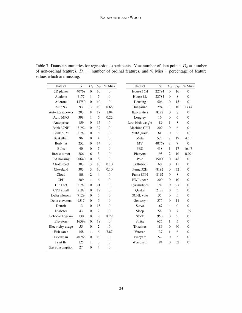
Table 7: Dataset summaries for regression experiments. N = number of data points, Dc = numberof non-ordinal features, Dr = number of ordinal features, and % Miss = percentage of featurevalues which are missing.

Dataset N Dc Dr % Miss

2D planes 40768 0 10 0Abalone 4177 1 7 0Ailerons 13750 0 40 0Auto 93 93 3 19 0.68

Auto horsepower 203 8 17 1.04Auto MPG 398 1 6 0.22Auto price 159 0 15 0

Bank 32NH 8192 0 32 0Bank 8FM 8192 0 8 0Basketball 96 0 4 0Body fat 252 0 14 0

Bolts 40 0 7 0Breast tumor 286 6 3 0CA housing 20640 0 8 0Cholesterol 303 3 10 0.10Cleveland 303 3 10 0.10

Cloud 108 2 4 0CPU 209 1 6 0

CPU act 8192 0 21 0CPU small 8192 0 12 0

Delta ailerons 7129 0 5 0Delta elevators 9517 0 6 0

Detroit 13 0 13 0Diabetes 43 0 2 0

Echocardiogram 130 0 9 8.29Elevators 16599 0 18 0

Electricity usage 55 0 2 0Fish catch 158 1 6 7.87Friedman 40768 0 10 0Fruit fly 125 1 3 0

Gas consumption 27 0 4 0

Dataset N Dc Dr % Miss

House 16H 22784 0 16 0House 8L 22784 0 8 0Housing 506 0 13 0

Hungarian 294 3 10 13.47Kinematics 8192 0 8 0

Longley 16 0 6 0Low birth weight 189 1 8 0

Machine CPU 209 0 6 0MBA grade 61 0 2 0

Meta 528 2 19 4.55MV 40768 3 7 0PBC 418 1 17 16.47

Pharynx 195 2 10 0.09Pole 15000 0 48 0

Pollution 60 0 15 0Puma 32H 8192 0 32 0Puma 8NH 8192 0 8 0PW Linear 200 0 10 0Pyrimidines 74 0 27 0

Quake 2178 0 3 0SCHL vote 37 0 5 0

Sensory 576 0 11 0Servo 167 4 0 0Sleep 58 0 7 1.97Stock 950 0 9 0Strike 625 1 5 0

Triazines 186 0 60 0Veteran 137 1 6 0

Vineyard 52 0 3 0Wisconsin 194 0 32 0

24

CANONICAL CORRELATION FORESTS

Table 8: Mean squared error as a percentage of the data variance. Conventions as per Table 2.

Dataset CCF RF Rot For CCF-Bag RRF RRF-Bag2D planes 6.37 ± 0.12 5.57 ± 0.10 5.87 ± 0.11 6.09 ± 0.11 6.57 ± 0.12 • 6.08 ± 0.11 Abalone 40.83 ± 4.91 43.88 ± 5.39 • 42.08 ± 5.11 • 40.72 ± 4.86 43.62 ± 5.18 • 43.24 ± 5.16 •Ailerons 17.46 ± 1.15 18.60 ± 1.24 • 17.23 ± 1.10 17.48 ± 1.14 19.03 ± 1.30 • 19.74 ± 1.35 •Auto 93 27.31 ± 32.94 34.42 ± 38.42 • 34.92 ± 34.50 • 28.15 ± 34.09 • 30.46 ± 35.70 • 34.41 ± 39.39 •

Auto horsepower 10.89 ± 14.89 15.37 ± 18.44 • 12.11 ± 15.11 • 11.23 ± 15.10 • 13.21 ± 16.42 • 15.00 ± 17.55 •Auto MPG 11.53 ± 4.56 12.61 ± 5.44 • 11.85 ± 4.91 • 11.68 ± 4.53 • 11.44 ± 4.73 11.89 ± 4.82 •Auto price 10.91 ± 7.57 12.20 ± 9.60 • 11.83 ± 9.62 • 11.95 ± 8.57 • 12.75 ± 11.81 • 14.59 ± 13.41 •

Bank 32NH 48.67 ± 3.83 50.35 ± 3.94 • 48.61 ± 3.88 48.89 ± 3.82 • 52.50 ± 4.02 • 53.59 ± 4.05 •Bank 8FM 3.70 ± 0.25 4.19 ± 0.29 • 4.38 ± 0.27 • 3.74 ± 0.25 • 4.58 ± 0.28 • 4.86 ± 0.30 •Basketball 72.77 ± 31.73 69.98 ± 34.67 66.38 ± 30.50 69.77 ± 31.60 73.88 ± 31.73 • 69.79 ± 31.75 Body fat 4.73 ± 3.26 5.41 ± 3.47 • 4.95 ± 3.51 5.36 ± 3.34 • 10.06 ± 4.31 • 11.55 ± 4.75 •

Bolts 8.62 ± 8.05 10.57 ± 7.58 • 17.45 ± 13.24 • 10.61 ± 9.66 • 22.32 ± 17.85 • 24.61 ± 19.00 •Breast tumor 108.1 ± 25.03 99.96 ± 23.73 98.19 ± 23.15 104.8 ± 24.13 115.0 ± 26.53 • 105.3 ± 24.86 CA housing 19.46 ± 1.13 17.55 ± 1.08 20.29 ± 1.17 • 19.65 ± 1.13 • 21.33 ± 1.19 • 21.90 ± 1.20 •Cholesterol 99.71 ± 43.48 99.56 ± 43.08 97.62 ± 41.95 99.25 ± 43.31 101.1 ± 44.32 • 98.53 ± 43.85 Cleveland 48.15 ± 14.20 49.64 ± 14.68 • 48.31 ± 15.15 47.80 ± 13.85 48.95 ± 14.15 • 48.71 ± 13.89 •

Cloud 22.09 ± 22.59 20.65 ± 23.51 26.19 ± 28.85 • 21.65 ± 23.65 24.08 ± 27.58 • 25.98 ± 29.25 •CPU 8.07 ± 20.08 13.93 ± 28.85 • 12.95 ± 42.08 10.28 ± 22.11 • 12.06 ± 26.98 • 17.20 ± 32.16 •

CPU act 1.66 ± 0.14 1.75 ± 0.19 • 1.77 ± 0.23 • 1.71 ± 0.15 • 2.63 ± 0.43 • 2.97 ± 0.52 •CPU small 2.25 ± 0.19 2.30 ± 0.24 • 2.45 ± 0.26 • 2.29 ± 0.19 • 2.45 ± 0.22 • 2.59 ± 0.24 •

Delta ailerons 28.70 ± 2.44 28.30 ± 2.64 30.31 ± 3.00 • 28.53 ± 2.45 28.99 ± 2.64 • 28.76 ± 2.67Delta elevators 36.40 ± 2.20 36.74 ± 2.28 • 35.41 ± 2.24 36.04 ± 2.19 36.75 ± 2.25 • 36.01 ± 2.23

Detroit 39.20 ± 78.01 43.25 ± 75.49 • 102.5 ± 125.6 • 44.25 ± 90.56 • 35.72 ± 68.25 41.68 ± 82.03 •Diabetes 70.84 ± 45.65 64.93 ± 39.75 87.56 ± 54.48 • 71.01 ± 45.74 67.54 ± 43.10 67.77 ± 43.06

Echocardiogram 56.94 ± 19.42 54.11 ± 18.47 52.09 ± 17.91 56.53 ± 18.79 58.00 ± 19.32 • 56.82 ± 18.33Elevators 10.34 ± 1.01 18.39 ± 1.76 • 14.81 ± 1.45 • 10.46 ± 1.03 • 20.03 ± 2.06 • 21.57 ± 2.22 •

Electricity usage 21.29 ± 13.25 22.25 ± 14.09 28.82 ± 22.79 • 21.23 ± 13.34 23.54 ± 16.33 23.55 ± 16.40Fish catch 2.17 ± 2.35 6.15 ± 7.20 • 5.40 ± 10.14 • 2.55 ± 2.66 • 3.24 ± 3.33 • 4.59 ± 4.83 •Friedman 9.15 ± 0.19 6.60 ± 0.17 7.36 ± 0.21 9.28 ± 0.20 • 8.66 ± 0.22 9.40 ± 0.24 •Fruit fly 128.6 ± 66.66 124.0 ± 67.16 108.0 ± 65.43 123.4 ± 65.91 136.6 ± 68.94 • 126.2 ± 66.98

Gas consumption 4.02 ± 4.68 6.71 ± 7.05 • 10.08 ± 6.80 • 4.69 ± 6.90 5.83 ± 5.37 • 5.81 ± 7.25 •House 16H 36.57 ± 4.47 35.74 ± 4.49 40.51 ± 4.88 • 37.04 ± 4.42 • 40.30 ± 4.68 • 41.98 ± 4.83 •House 8L 29.96 ± 3.11 30.53 ± 3.13 • 32.94 ± 3.41 • 30.08 ± 3.10 • 31.89 ± 3.26 • 32.28 ± 3.29 •Housing 12.89 ± 8.47 13.51 ± 9.04 • 14.86 ± 9.56 • 13.49 ± 8.68 • 13.85 ± 8.93 • 15.42 ± 9.63 •

Hungarian 50.94 ± 14.55 55.42 ± 15.34 • 53.94 ± 16.01 • 50.22 ± 14.54 51.04 ± 14.30 51.06 ± 13.76Kinematics 20.33 ± 1.05 27.97 ± 1.46 • 21.33 ± 1.16 • 20.92 ± 1.09 • 18.81 ± 1.00 20.98 ± 1.10 •

Longley 6.61 ± 7.56 14.75 ± 12.00 • 16.67 ± 17.19 • 8.77 ± 9.75 • 9.57 ± 8.02 • 14.32 ± 10.72 •Low birth weight 40.09 ± 13.68 39.63 ± 12.92 37.97 ± 13.03 38.89 ± 13.27 45.71 ± 16.38 • 43.58 ± 15.95 •

Machine CPU 12.80 ± 23.68 16.69 ± 30.55 • 23.39 ± 37.67 • 14.79 ± 24.89 • 13.10 ± 26.48 17.53 ± 30.16 •MBA grade 106.1 ± 69.36 106.0 ± 68.30 91.00 ± 66.94 107.0 ± 69.62 • 106.5 ± 68.01 107.3 ± 68.51

Meta 93.29 ± 159.3 95.34 ± 165.4 • 100.3 ± 185.3 95.28 ± 165.6 97.12 ± 175.6 99.64 ± 184.7MV 0.00 ± 0.00 0.02 ± 0.01 • 0.02 ± 0.00 • 0.00 ± 0.00 • 0.29 ± 0.01 • 0.36 ± 0.02 •PBC 62.81 ± 12.95 65.11 ± 13.09 • 60.50 ± 13.39 62.45 ± 12.79 64.24 ± 13.04 • 65.00 ± 13.14 •

Pharynx 36.35 ± 16.41 37.24 ± 17.90 • 32.47 ± 17.89 37.83 ± 16.34 • 46.21 ± 19.35 • 49.02 ± 19.39 •Pole 2.43 ± 0.21 2.78 ± 0.22 • 1.27 ± 0.12 2.65 ± 0.23 • 2.25 ± 0.21 2.75 ± 0.23 •

Pollution 43.35 ± 30.47 48.87 ± 34.14 • 47.37 ± 31.65 • 43.75 ± 30.44 47.81 ± 32.00 • 50.93 ± 34.02 •Puma 32H 65.10 ± 3.48 26.07 ± 1.76 14.59 ± 0.93 67.43 ± 3.53 • 66.53 ± 3.19 • 69.08 ± 3.30 •Puma 8NH 32.68 ± 1.77 32.64 ± 1.81 33.18 ± 1.78 • 32.60 ± 1.76 34.93 ± 1.86 • 35.59 ± 1.83 •PW Linear 15.33 ± 5.61 16.66 ± 6.09 • 15.19 ± 5.55 15.86 ± 5.83 • 21.26 ± 8.34 • 24.02 ± 9.18 •Pyrimidines 58.21 ± 113.2 63.96 ± 125.5 • 69.33 ± 115.6 • 59.33 ± 115.8 • 57.73 ± 113.2 60.47 ± 112.8 •

Quake 106.1 ± 11.97 105.2 ± 11.57 99.75 ± 11.67 103.0 ± 11.51 109.6 ± 12.23 • 104.5 ± 11.60 SCHL vote 78.31 ± 141.5 58.17 ± 125.3 93.58 ± 179.9 76.87 ± 140.8 75.34 ± 137.8 79.09 ± 147.0

Sensory 77.27 ± 12.74 70.44 ± 11.72 71.99 ± 11.75 77.80 ± 12.83 • 77.44 ± 12.77 78.74 ± 13.20 •Servo 10.93 ± 14.87 13.85 ± 18.54 • 14.75 ± 20.91 • 12.34 ± 14.96 • 18.54 ± 19.51 • 23.10 ± 20.77 •Sleep 48.24 ± 23.37 56.58 ± 24.68 • 53.74 ± 25.09 • 48.00 ± 22.71 48.21 ± 24.02 48.82 ± 22.74Stock 1.11 ± 0.22 1.35 ± 0.34 • 1.27 ± 0.26 • 1.25 ± 0.25 • 1.06 ± 0.23 1.27 ± 0.26 •Strike 87.35 ± 100.0 84.22 ± 99.55 90.00 ± 102.2 • 87.84 ± 99.23 87.19 ± 101.0 85.03 ± 100.8

Triazines 71.99 ± 36.69 71.01 ± 35.37 70.25 ± 34.49 71.56 ± 36.57 72.44 ± 36.78 72.87 ± 37.27 •Veteran 80.39 ± 77.45 88.10 ± 88.31 • 84.10 ± 89.71 78.38 ± 73.80 79.03 ± 78.11 78.35 ± 77.85

Vineyard 34.86 ± 27.98 36.99 ± 33.40 46.64 ± 32.90 • 35.52 ± 28.49 • 34.77 ± 28.92 35.50 ± 31.08Wisconsin 87.82 ± 24.18 92.91 ± 24.91 • 90.38 ± 24.95 • 87.33 ± 23.96 89.87 ± 25.33 • 88.52 ± 24.80

25

RAINFORTH AND WOOD

Table 9: Number of victories column vs row at 1% significance level of Wilcoxon signed rank testfor regression experiments (61 total). CCF victories and losses are given in blue and red respectively.

CCF RF Rotation Forest CCF-Bag RRF RRF-Bag

CCF - 16 17 17 8 10RF 38 - 28 31 17 13Rotation Forest 35 24 - 31 22 16CCF-Bag 33 13 18 - 11 3RRF 41 31 32 40 - 13RRF-Bag 41 33 36 41 38 -

Table 10: Mean rank across datasets of test mean squared error. Lower rank corresponds to betterperformance.

Algorithm Mean Rank

CCF 2.43CCF-Bag 2.67Rotation Forest 3.56RF 3.64RRF 4.02RRF-Bag 4.69

6. Multiple Outputs

We now demonstrate how CCFs can be used for multiple output problems such as multivariate re-gression, where we wish to regress multiple outputs simultaneously, and multi-output classification,where we wish to learn a single estimator to predict multiple classification tasks. We note that multi-label classification, where we wish to predict a number of classes which are not mutually exclusive,can be thought of as a special case of multi-output classification were all of the classification tasksare binary. In principle, CCFs can also handle problems with arbitrary combinations of classifica-tion and regression outputs in the same way as RFs (see e.g. Glocker et al. (2012); Linusson (2013)),but we will not actively consider this case further here.

Various multiple-output axis-aligned decision trees and forests have previously been developedin the literature (Zhang, 1998; De’Ath, 2002; Geurts et al., 2006b; Segal and Xiao, 2011; Glockeret al., 2012; Faddoul et al., 2012; Linusson, 2013). There are three key ways these approaches tendto vary from single axis aligned approaches: the calculation of split gains which must now assessthe utility of the split to multiple different tasks simultaneously, the leaf models which must nowpredict multiple outputs, and the manner in which the individual tree predictions are combined.

In the simplest case, the leafs have independent models for each of the outputs and the ensembleprediction for each output is the average over trees of the corresponding leaf predictions in thesame manner as the single output case. Improvements on this approach have been suggested. Forexample, Geurts et al. (2006b) introduce the idea of kernelizing the decision tree outputs to ensurethe ensemble prediction respects the structure of the output data. As these ideas apply equally

26

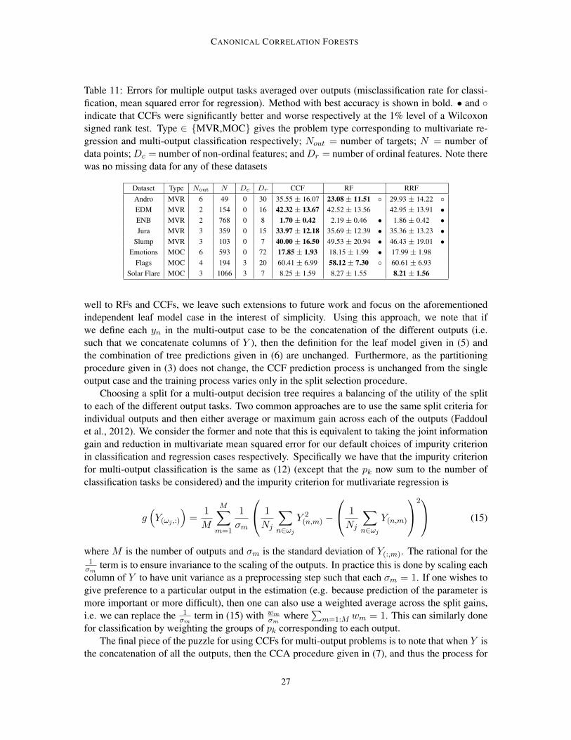
CANONICAL CORRELATION FORESTS

Table 11: Errors for multiple output tasks averaged over outputs (misclassification rate for classi-fication, mean squared error for regression). Method with best accuracy is shown in bold. • and indicate that CCFs were significantly better and worse respectively at the 1% level of a Wilcoxonsigned rank test. Type ∈ MVR,MOC gives the problem type corresponding to multivariate re-gression and multi-output classification respectively; Nout = number of targets; N = number ofdata points; Dc = number of non-ordinal features; andDr = number of ordinal features. Note therewas no missing data for any of these datasets

Dataset Type Nout N Dc Dr CCF RF RRFAndro MVR 6 49 0 30 35.55 ± 16.07 23.08 ± 11.51 29.93 ± 14.22 EDM MVR 2 154 0 16 42.32 ± 13.67 42.52 ± 13.56 42.95 ± 13.91 •ENB MVR 2 768 0 8 1.70 ± 0.42 2.19 ± 0.46 • 1.86 ± 0.42 •Jura MVR 3 359 0 15 33.97 ± 12.18 35.69 ± 12.39 • 35.36 ± 13.23 •

Slump MVR 3 103 0 7 40.00 ± 16.50 49.53 ± 20.94 • 46.43 ± 19.01 •Emotions MOC 6 593 0 72 17.85 ± 1.93 18.15 ± 1.99 • 17.99 ± 1.98

Flags MOC 4 194 3 20 60.41 ± 6.99 58.12 ± 7.30 60.61 ± 6.93Solar Flare MOC 3 1066 3 7 8.25 ± 1.59 8.27 ± 1.55 8.21 ± 1.56

well to RFs and CCFs, we leave such extensions to future work and focus on the aforementionedindependent leaf model case in the interest of simplicity. Using this approach, we note that ifwe define each yn in the multi-output case to be the concatenation of the different outputs (i.e.such that we concatenate columns of Y ), then the definition for the leaf model given in (5) andthe combination of tree predictions given in (6) are unchanged. Furthermore, as the partitioningprocedure given in (3) does not change, the CCF prediction process is unchanged from the singleoutput case and the training process varies only in the split selection procedure.

Choosing a split for a multi-output decision tree requires a balancing of the utility of the splitto each of the different output tasks. Two common approaches are to use the same split criteria forindividual outputs and then either average or maximum gain across each of the outputs (Faddoulet al., 2012). We consider the former and note that this is equivalent to taking the joint informationgain and reduction in multivariate mean squared error for our default choices of impurity criterionin classification and regression cases respectively. Specifically we have that the impurity criterionfor multi-output classification is the same as (12) (except that the pk now sum to the number ofclassification tasks be considered) and the impurity criterion for mutlivariate regression is

g(Y(ωj ,:)

)=

1

M

M∑m=1

1

σm

1

Nj

∑n∈ωj

Y 2(n,m) −

1

Nj

∑n∈ωj

Y(n,m)

2 (15)

where M is the number of outputs and σm is the standard deviation of Y(:,m). The rational for the1σm

term is to ensure invariance to the scaling of the outputs. In practice this is done by scaling eachcolumn of Y to have unit variance as a preprocessing step such that each σm = 1. If one wishes togive preference to a particular output in the estimation (e.g. because prediction of the parameter ismore important or more difficult), then one can also use a weighted average across the split gains,i.e. we can replace the 1

σmterm in (15) with wm

σmwhere

∑m=1:M wm = 1. This can similarly done

for classification by weighting the groups of pk corresponding to each output.The final piece of the puzzle for using CCFs for multi-output problems is to note that when Y is

the concatenation of all the outputs, then the CCA procedure given in (7), and thus the process for

27

RAINFORTH AND WOOD

calculating Φ, is unchanged. This seamless transition is an advantage to our choice of using CCAprojections. In theory, one could also make use the canonical components of the outputs for themulti-output case. However, preliminary investigation suggests that a naıve approach, where theseare used for the split criterion rather than the original outputs, is not beneficial.

To assess the performance of CCFs for multi-output problems we considered a selection ofdatasets taken from the Mulan10 (Tsoumakas et al., 2010) and UCI (Lichman, 2013) databases. Theexperimental procedures was as for the single output experiments (using the same respective defaultparameters for regression and classification) and we make comparisons to RF and RRF. As the RFpackage used previously does not support multiple outputs, an adaptation of our CCF package wasused instead. Dataset summaries and results are shown in Table 11 with win/draw/loss ratios forCCFs of 4/2/2 and 4/3/1 compared to RFs and RRFs respectively. More extensive investigationis necessary to fully assess the relative merit of CCFs compared to alternatives for multi-outputproblems, but these results are promising and suggest gains transfer from the single output case.

7. Discussion

7.1 Effect of Correlation between Input Features

As shown by Menze et al. (2011), RFs often struggle on data with highly correlated features. CCAnaturally incorporates information about feature correlations, therefore CCFs do not suffer the sameissues. This is demonstrated, for example, by their superior performance on the highly correlatedhill valley datasets.

To more rigorously investigate the effect of correlation, we used the following method of artifi-cially correlating the data (after carrying out the preprocessing described in Section 3.3.2):

1. Add a new random feature

X(D+1,n) ∼ N (0, κ) , ∀n = 1, . . . , N

where κ is a parameter which will control the degree of correlation to be added.

2. To each of the existing features, randomly either add or subtract the new feature, i.e.

X(:,d) ← X(:,d) + ζdX(:,D+1), ∀d = 1, . . . , D

where each ζdi.i.d∼ UNIFORM-DISCRETE −1, 1.

As shown in Figure 5, this transformation has no effect on the accuracy of CCFs, whereas the accu-racy of RF decreases with increasing κ, eventually giving the same accuracy as random prediction.We also see that RRF fare only marginally better than RF under this artificial correlation. The useof PCA means rotation forests, on the other hand, exhibit similar robustness to global correlationsas CCFs.

We postulate that CCFs are better than rotation forests at incorporating class dependent andlocalized correlations. This is because the rotation step of rotation forests does not incorporateany class information other than in the random elimination of classes. Further, individual trees ina rotation forest are orthogonal and therefore cannot incorporate spatial variation in correlation.The self similar nature of the growth algorithm for CCTs, on the other hand, means that the localcorrelations of a partition can be incorporated as naturally as the global correlations.

10. http://mulan.sourceforge.net/datasets-mtr.html

28

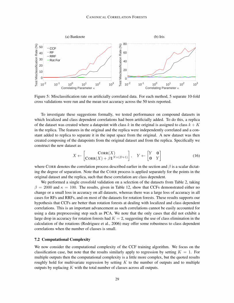
CANONICAL CORRELATION FORESTS

(a) Banknote

Correlating Parameter 510-2 10-1 100 101 102 103

Tes

t Mis

clas

sific

atio

n R

ate

(%)

0

10

20

30

40

50 CCF RF RRF Rot For

(b) Iris

Correlating Parameter 510-2 10-1 100 101 102 103

Tes

t Mis

clas

sific

atio

n R

ate

(%)

0

20

40

60

80

Figure 5: Misclassification rate on artificially correlated data. For each method, 5 separate 10-foldcross validations were run and the mean test accuracy across the 50 tests reported.

To investigate these suggestions formally, we tested performance on compound datasets inwhich localized and class dependent correlations had been artificially added. To do this, a replicaof the dataset was created where a datapoint with class k in the original is assigned to class k + Kin the replica. The features in the original and the replica were independently correlated and a con-stant added to replica to separate it in the input space from the original. A new dataset was thencreated composing of the datapoints from the original dataset and from the replica. Specifically weconstruct the new dataset as

X ←[

CORR(X)

CORR(X) + β1N×(D+1)

], Y ←

[Y 00 Y

](16)

where CORR denotes the correlation process described earlier in the section and β is a scalar dictat-ing the degree of separation. Note that the CORR process is applied separately for the points in theoriginal dataset and the replica, such that these correlation are class dependent.

We performed a single crossfold validation on a selection of the datasets from Table 2, takingβ = 2000 and κ = 100. The results, given in Table 12, show that CCFs demonstrated either nochange or a small loss in accuracy on all datasets, whereas there was a large loss of accuracy in allcases for RFs and RRFs, and on most of the datasets for rotation forests. These results supports ourhypothesis that CCFs are better than rotation forests at dealing with localized and class dependentcorrelations. This is an important advancement as such correlations cannot be easily accounted forusing a data preprocessing step such as PCA. We note that the only cases that did not exhibit alarge drop in accuracy for rotation forests had K = 2, suggesting the use of class elimination in thecalculation of the rotations (Rodriguez et al., 2006) may offer some robustness to class dependentcorrelations when the number of classes is small.

7.2 Computational Complexity

We now consider the computational complexity of the CCF training algorithm. We focus on theclassification case, but note that the results similarly apply to regression by setting K = 1. Formultiple outputs then the computational complexity is a little more complex, but the quoted resultsroughly hold for multivariate regression by setting K to the number of outputs and to multipleoutputs by replacing K with the total number of classes across all outputs.

29

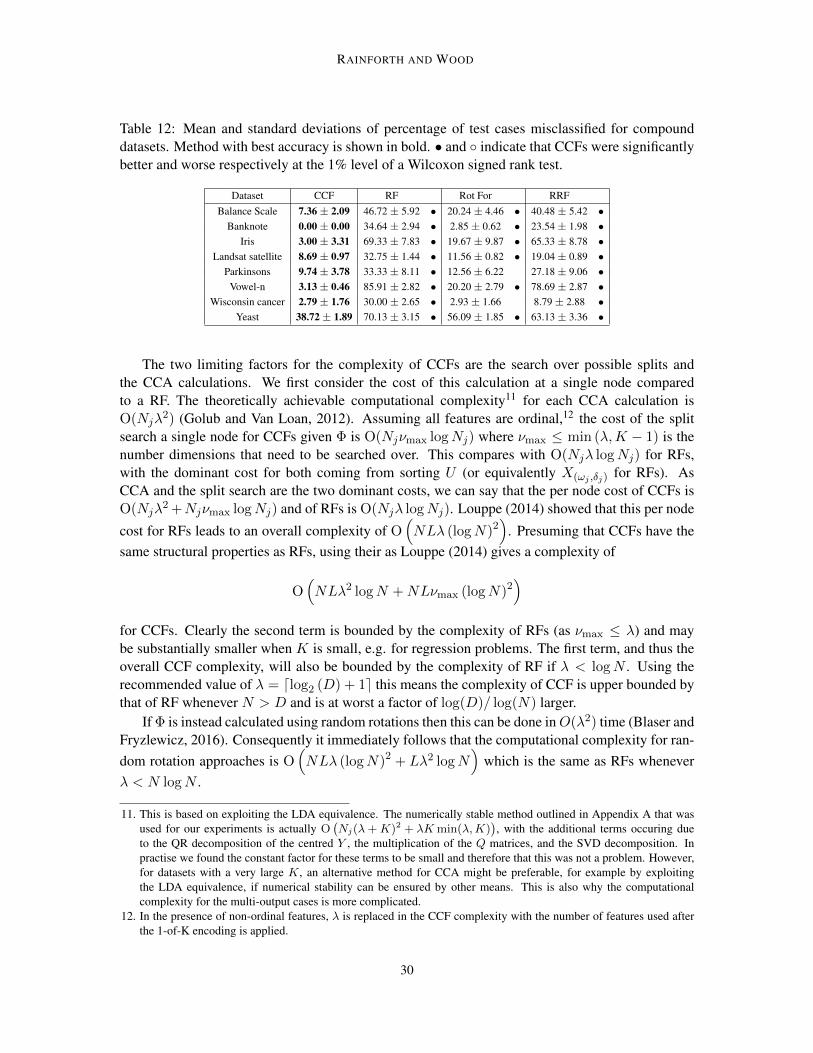
RAINFORTH AND WOOD

Table 12: Mean and standard deviations of percentage of test cases misclassified for compounddatasets. Method with best accuracy is shown in bold. • and indicate that CCFs were significantlybetter and worse respectively at the 1% level of a Wilcoxon signed rank test.

Dataset CCF RF Rot For RRFBalance Scale 7.36 ± 2.09 46.72 ± 5.92 • 20.24 ± 4.46 • 40.48 ± 5.42 •

Banknote 0.00 ± 0.00 34.64 ± 2.94 • 2.85 ± 0.62 • 23.54 ± 1.98 •Iris 3.00 ± 3.31 69.33 ± 7.83 • 19.67 ± 9.87 • 65.33 ± 8.78 •

Landsat satellite 8.69 ± 0.97 32.75 ± 1.44 • 11.56 ± 0.82 • 19.04 ± 0.89 •Parkinsons 9.74 ± 3.78 33.33 ± 8.11 • 12.56 ± 6.22 27.18 ± 9.06 •

Vowel-n 3.13 ± 0.46 85.91 ± 2.82 • 20.20 ± 2.79 • 78.69 ± 2.87 •Wisconsin cancer 2.79 ± 1.76 30.00 ± 2.65 • 2.93 ± 1.66 8.79 ± 2.88 •

Yeast 38.72 ± 1.89 70.13 ± 3.15 • 56.09 ± 1.85 • 63.13 ± 3.36 •

The two limiting factors for the complexity of CCFs are the search over possible splits andthe CCA calculations. We first consider the cost of this calculation at a single node comparedto a RF. The theoretically achievable computational complexity11 for each CCA calculation isO(Njλ

2) (Golub and Van Loan, 2012). Assuming all features are ordinal,12 the cost of the splitsearch a single node for CCFs given Φ is O(Njνmax logNj) where νmax ≤ min (λ,K − 1) is thenumber dimensions that need to be searched over. This compares with O(Njλ logNj) for RFs,with the dominant cost for both coming from sorting U (or equivalently X(ωj ,δj) for RFs). AsCCA and the split search are the two dominant costs, we can say that the per node cost of CCFs isO(Njλ

2 +Njνmax logNj) and of RFs is O(Njλ logNj). Louppe (2014) showed that this per node

cost for RFs leads to an overall complexity of O(NLλ (logN)2

). Presuming that CCFs have the

same structural properties as RFs, using their as Louppe (2014) gives a complexity of

O(NLλ2 logN +NLνmax (logN)2

)for CCFs. Clearly the second term is bounded by the complexity of RFs (as νmax ≤ λ) and maybe substantially smaller when K is small, e.g. for regression problems. The first term, and thus theoverall CCF complexity, will also be bounded by the complexity of RF if λ < logN . Using therecommended value of λ = dlog2 (D) + 1e this means the complexity of CCF is upper bounded bythat of RF whenever N > D and is at worst a factor of log(D)/ log(N) larger.

If Φ is instead calculated using random rotations then this can be done inO(λ2) time (Blaser andFryzlewicz, 2016). Consequently it immediately follows that the computational complexity for ran-dom rotation approaches is O

(NLλ (logN)2 + Lλ2 logN

)which is the same as RFs whenever

λ < N logN .

11. This is based on exploiting the LDA equivalence. The numerically stable method outlined in Appendix A that wasused for our experiments is actually O

(Nj(λ+K)2 + λKmin(λ,K)

), with the additional terms occuring due

to the QR decomposition of the centred Y , the multiplication of the Q matrices, and the SVD decomposition. Inpractise we found the constant factor for these terms to be small and therefore that this was not a problem. However,for datasets with a very large K, an alternative method for CCA might be preferable, for example by exploitingthe LDA equivalence, if numerical stability can be ensured by other means. This is also why the computationalcomplexity for the multi-output cases is more complicated.

12. In the presence of non-ordinal features, λ is replaced in the CCF complexity with the number of features used afterthe 1-of-K encoding is applied.

30

CANONICAL CORRELATION FORESTS

Rotation forest training requires each tree to search the full set of features and therefore has atraining complexity of O

(NLD (logN)2

). This is exponentially more expensive in the number

of features than RFs and CCFs when λ is set to a logarithmic factor of D. This makes their imple-mentation impractical for datasets with more than a modest number of features, as demonstrated bythe ORL and polya datasets for which we were unable to carry out most tests with rotation forests,experiencing both memory issues and an impractically long training time.

Should one wish to use CCFs with a λ that is significantly larger than the suggested default,speeds gains should be achievable by separately generating M projection matrices Φmm=1:M ,each using λ/M features, and searching for the optimal split over all generated projections. WhenK is small, such an approach could also be used to increase the size of the set of candidate splits gen-erated and might therefore also be beneficial to performance in some scenarios. We leave assessingthe effect of this change on predictive performance to future work.

7.3 Empirical Run Times

To more explicitly evaluate the practical speed of CCFs compared to competitors, we now considerempirical run times. To ensure fair comparison, we used our code base for the CCF, CCF-Bag, RRF,and RRF-Bag implementations for calculating the RFs and rotation forests timings. All methodsthus shared the same code except in the calculation of Φ (which is just set to an identity matrix forRFs and rotation forests), whether bagging is used, and the tree projection calculation and differentvalue of λ required for rotation forests. Runs were carried out on a single machine with 64 AMDOpteron 1.4GHz processors and using 2 threads per core.

Table 13 shows the absolute run times for CCFs and the run times of the alternatives as a ratio ofthe corresponding CCF run time. To characterise whether changes originate from differences in thesize of the learnt trees, the average number of nodes for each tree are also shown. As expected, therun times for rotation forests were significantly larger that the other algorithms for any datasets withmore than a few input features. CCF-Bag was (marginally) faster than CCFs and produced smallertrees, as would also be expected because bagging reduces the effective size of the dataset each treeis trained on. Perhaps surprisingly though, RFs, RRFs, and RRF-Bag were all substantially slowerthan CCFs, each having longer run times on every dataset except spirals and respectively takingon average 1.92, 2.03, and 1.83 times longer to run than CCFs. These numbers rise further to2.57, 2.62, and 2.35 respectively if one omits time spent on parallelization overheads. Althoughthe relative speeds will of course vary between implementations, these results suggest not only doCCFs offer better predictive accuracy than the alternatives, they are faster to train as well.

Though occasionally producing substantially larger trees, RFs and RRF-Bag more often than notproduced smaller trees than CCFs, again presumably because of the reduction in effective trainingdataset size caused by bagging. The speed differences for these algorithms cannot thus originatepredominantly from changes in the tree size. CCFs are in fact faster because they consider, onaverage, a smaller number of candidate splits than the other approaches, with the cost of searchingof these splits typically being larger than the cost of carrying out CCA. This is easy to see in thecase were K < λ as CCFs search over νmax ≤ max(K,λ) projections, compared to λ for thealternatives. Somewhat more subtly, then this effect still occurs for the tree as a whole even whenK > λ. Although it is still necessary to search over λ splits at the root of the tree when K > λ, thepartitioning procedure attempts to create the “purest” possible children and so the average numberof classes present at a node decreases the deeper one goes down the tree. As νmax for a particular

31

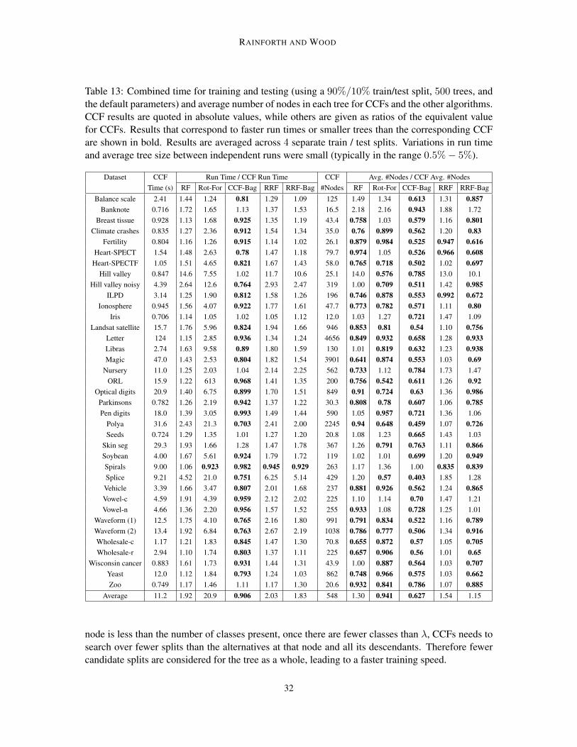
RAINFORTH AND WOOD

Table 13: Combined time for training and testing (using a 90%/10% train/test split, 500 trees, andthe default parameters) and average number of nodes in each tree for CCFs and the other algorithms.CCF results are quoted in absolute values, while others are given as ratios of the equivalent valuefor CCFs. Results that correspond to faster run times or smaller trees than the corresponding CCFare shown in bold. Results are averaged across 4 separate train / test splits. Variations in run timeand average tree size between independent runs were small (typically in the range 0.5%− 5%).

Dataset CCF Run Time / CCF Run Time CCF Avg. #Nodes / CCF Avg. #NodesTime (s) RF Rot-For CCF-Bag RRF RRF-Bag #Nodes RF Rot-For CCF-Bag RRF RRF-Bag

Balance scale 2.41 1.44 1.24 0.81 1.29 1.09 125 1.49 1.34 0.613 1.31 0.857Banknote 0.716 1.72 1.65 1.13 1.37 1.53 16.5 2.18 2.16 0.943 1.88 1.72

Breast tissue 0.928 1.13 1.68 0.925 1.35 1.19 43.4 0.758 1.03 0.579 1.16 0.801Climate crashes 0.835 1.27 2.36 0.912 1.54 1.34 35.0 0.76 0.899 0.562 1.20 0.83

Fertility 0.804 1.16 1.26 0.915 1.14 1.02 26.1 0.879 0.984 0.525 0.947 0.616Heart-SPECT 1.54 1.48 2.63 0.78 1.47 1.18 79.7 0.974 1.05 0.526 0.966 0.608

Heart-SPECTF 1.05 1.51 4.65 0.821 1.67 1.43 58.0 0.765 0.718 0.502 1.02 0.697Hill valley 0.847 14.6 7.55 1.02 11.7 10.6 25.1 14.0 0.576 0.785 13.0 10.1

Hill valley noisy 4.39 2.64 12.6 0.764 2.93 2.47 319 1.00 0.709 0.511 1.42 0.985ILPD 3.14 1.25 1.90 0.812 1.58 1.26 196 0.746 0.878 0.553 0.992 0.672

Ionosphere 0.945 1.56 4.07 0.922 1.77 1.61 47.7 0.773 0.782 0.571 1.11 0.80Iris 0.706 1.14 1.05 1.02 1.05 1.12 12.0 1.03 1.27 0.721 1.47 1.09

Landsat satellite 15.7 1.76 5.96 0.824 1.94 1.66 946 0.853 0.81 0.54 1.10 0.756Letter 124 1.15 2.85 0.936 1.34 1.24 4656 0.849 0.932 0.658 1.28 0.933Libras 2.74 1.63 9.58 0.89 1.80 1.59 130 1.01 0.819 0.632 1.23 0.938Magic 47.0 1.43 2.53 0.804 1.82 1.54 3901 0.641 0.874 0.553 1.03 0.69

Nursery 11.0 1.25 2.03 1.04 2.14 2.25 562 0.733 1.12 0.784 1.73 1.47ORL 15.9 1.22 613 0.968 1.41 1.35 200 0.756 0.542 0.611 1.26 0.92

Optical digits 20.9 1.40 6.75 0.899 1.70 1.51 849 0.91 0.724 0.63 1.36 0.986Parkinsons 0.782 1.26 2.19 0.942 1.37 1.22 30.3 0.808 0.78 0.607 1.06 0.785Pen digits 18.0 1.39 3.05 0.993 1.49 1.44 590 1.05 0.957 0.721 1.36 1.06

Polya 31.6 2.43 21.3 0.703 2.41 2.00 2245 0.94 0.648 0.459 1.07 0.726Seeds 0.724 1.29 1.35 1.01 1.27 1.20 20.8 1.08 1.23 0.665 1.43 1.03

Skin seg 29.3 1.93 1.66 1.28 1.47 1.78 367 1.26 0.791 0.763 1.11 0.866Soybean 4.00 1.67 5.61 0.924 1.79 1.72 119 1.02 1.01 0.699 1.20 0.949Spirals 9.00 1.06 0.923 0.982 0.945 0.929 263 1.17 1.36 1.00 0.835 0.839Splice 9.21 4.52 21.0 0.751 6.25 5.14 429 1.20 0.57 0.403 1.85 1.28Vehicle 3.39 1.66 3.47 0.807 2.01 1.68 237 0.881 0.926 0.562 1.24 0.865Vowel-c 4.59 1.91 4.39 0.959 2.12 2.02 225 1.10 1.14 0.70 1.47 1.21Vowel-n 4.66 1.36 2.20 0.956 1.57 1.52 255 0.933 1.08 0.728 1.25 1.01

Waveform (1) 12.5 1.75 4.10 0.765 2.16 1.80 991 0.791 0.834 0.522 1.16 0.789Waveform (2) 13.4 1.92 6.84 0.763 2.67 2.19 1038 0.786 0.777 0.506 1.34 0.916Wholesale-c 1.17 1.21 1.83 0.845 1.47 1.30 70.8 0.655 0.872 0.57 1.05 0.705Wholesale-r 2.94 1.10 1.74 0.803 1.37 1.11 225 0.657 0.906 0.56 1.01 0.65

Wisconsin cancer 0.883 1.61 1.73 0.931 1.44 1.31 43.9 1.00 0.887 0.564 1.03 0.707Yeast 12.0 1.12 1.84 0.793 1.24 1.03 862 0.748 0.966 0.575 1.03 0.662Zoo 0.749 1.17 1.46 1.11 1.17 1.30 20.6 0.932 0.841 0.786 1.07 0.885

Average 11.2 1.92 20.9 0.906 2.03 1.83 548 1.30 0.941 0.627 1.54 1.15

node is less than the number of classes present, once there are fewer classes than λ, CCFs needs tosearch over fewer splits than the alternatives at that node and all its descendants. Therefore fewercandidate splits are considered for the tree as a whole, leading to a faster training speed.

32

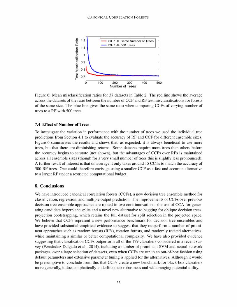
CANONICAL CORRELATION FORESTS

0 100 200 300 400 500

0.7

0.8

0.9

1

1.1

1.2

Number of Trees

Test

Mis

clas

sific

atio

n R

atio

CCF / RF Same Number of TreesCCF / RF 500 Trees

Figure 6: Mean misclassification ratios for 37 datasets in Table 2. The red line shows the averageacross the datasets of the ratio between the number of CCF and RF test misclassifications for forestsof the same size. The blue line gives the same ratio when comparing CCFs of varying number oftrees to a RF with 500 trees.

7.4 Effect of Number of Trees

To investigate the variation in performance with the number of trees we used the individual treepredictions from Section 4.1 to evaluate the accuracy of RF and CCF for different ensemble sizes.Figure 6 summarises the results and shows that, as expected, it is always beneficial to use moretrees, but that there are diminishing returns. Some datasets require more trees than others beforethe accuracy begins to saturate (not shown), but the advantages of CCFs over RFs is maintainedacross all ensemble sizes (though for a very small number of trees this is slightly less pronounced).A further result of interest is that on average it only takes around 15 CCTs to match the accuracy of500 RF trees. One could therefore envisage using a smaller CCF as a fast and accurate alternativeto a larger RF under a restricted computational budget.

8. Conclusions

We have introduced canonical correlation forests (CCFs), a new decision tree ensemble method forclassification, regression, and multiple output prediction. The improvements of CCFs over previousdecision tree ensemble approaches are rooted in two core innovations: the use of CCA for gener-ating candidate hyperplane splits and a novel new alternative to bagging for oblique decision trees,projection bootstrapping, which retains the full dataset for split selection in the projected space.We believe that CCFs represent a new performance benchmark for decision tree ensembles andhave provided substantial empirical evidence to suggest that they outperform a number of promi-nent approaches such as random forests (RFs), rotation forests, and randomly rotated alternatives,while maintaining a similar or better computational complexity. We have also provided evidencesuggesting that classification CCFs outperform all of the 179 classifiers considered in a recent sur-vey (Fernandez-Delgado et al., 2014), including a number of prominent SVM and neural networkpackages, over a large selection of datasets, even when CCFs are run in an out-of-box fashion usingdefault parameters and extensive parameter tuning is applied for the alternatives. Although it wouldbe presumptive to conclude from this that CCFs create a new benchmark for black-box classifiersmore generally, it does emphatically underline their robustness and wide ranging potential utility.

33

RAINFORTH AND WOOD

Acknowledgments

Tom Rainforth is supported by a BP industrial grant. Frank Wood is supported under DARPAPPAML through the U.S. AFRL under Cooperative Agreement number FA8750-14-2-0006, SubAward number 61160290-111668.

Appendix A. Numerically Stable CCA Algorithm

As explained in the main paper, the aim of CCA is to find pairs of linear projections Aν , Bνν=1:νmax

that maximize the correlations between two matrices W ∈ Rn×d and V ∈ Rn×k in the co-projectedspace WAν , V Bν. Let ΣWV be the cross covariance matrix betweenW and V such that the (i, j)entry of ΣWV (which we denote (ΣWV )(i,j)) is the empirical covariance between the ith column ofW and the jth column of V , namely

(ΣWV )(i,j) =1

N − 1

N∑n=1

(W(n,i) − Wi

)·(V(n,j) − Vj

)(17)

where Wi =1

N

N∑n=1

W(n,i), and Vj =1

N

N∑n=1

V(n,j).

Defining ΣWW and ΣV V in the same way, then a simple approach to calculate the canonical coef-ficients Aν , Bνν=1:νmax is to note that the satisfy (see e.g. Borga (2001))

Σ−1WWΣWV Σ−1

V V ΣVWAν = ρ2νAν

Σ−1V V ΣVWΣ−1

WWΣWVBν = ρ2νBν

(18)

such that they are the eigenvectors of Σ−1WWΣWV Σ−1

V V ΣVW and Σ−1V V ΣVWΣ−1

WWΣWV respectively.The common eigenvalues, which correspond to the squares of the canonical correlations ρν , makethe pairing between the coefficients of W and V apparent and the order of the coefficients is foundby the corresponding decreasing order of the canonical correlations, ρ1 ≥ ρ2 ≥ · · · ≥ ρνmax .

However, this solution can be numerically unstable as it requires an inversion of the often de-generate covariance matrices. We instead take the numerically stable approach laid out in Algorithm3, corresponding to the approach introduced by Bjorck and Golub (1973). Here [q, r, p] = QR(α)refers to a QR decomposition with pivoting such that qr = α(:,p) where q is an orthogonal ma-trix, r is upper triangular matrix and p is a column ordering defined implicitly such that |r (i, i)| >|r (j, j)| ∀i < j. [u,Ω, z] = SVD(α) refers to a singular value decomposition such that uΩzT = αwhere u and z are unitary matrix and Ω is diagonal matrix of singular values, with the ordering de-fined such that Ω (i, i) > Ω (j, j) ∀i < j.

After centring both inputs, a QR decomposition with pivoting is carried out on each. For exam-ple qr = wp where q is a unitary matrix, r is an upper triangular matrix and p is a pivot matrix suchthat the diagonal elements of p are of decreasing magnitude. If

ζ = maxi :∣∣r(i,i)

∣∣ > ε∣∣r(1,1)

∣∣ (19)

is the number of non-zero main diagonal terms within some tolerance ε, then the first ζ columnsof q will describe an orthonormal basis for the span of w. Therefore by applying the reductionsq′ ← q( : ,1:ζ) and r′ ← r(1:ζ,1:ζ), then q′r′ will be a pivoted reduction of w that is full rank and r′

34

CANONICAL CORRELATION FORESTS

Algorithm 3: Numerically Stable CCA

Inputs: First array w ∈ RN×D, second array v ∈ RN×K , tolerance parameter ε ∈ [0+, 1−]

Outputs: Projection matrices for first and second arrays A and B, correlations ρ1: µw = 1

N

∑n=1:N w(n,:), µv = 1

N

∑n=1:N v(n,:) . First centre the inputs

2: w(:,d) ← w(:,d) − µw(d) ∀d ∈ 1, . . . , D3: v(:,k) ← v(:,k) − µv(k) ∀k ∈ 1, . . . ,K4: [qw, rw, pw] = QR(w), [qv, rv, pv] = QR(v) . Carry out pivoted QR decompositions5: ζw = maxi : |rw(i,i)| < ε|rw(1,1)|, ζv = maxi : |rv(i,i)| < ε|rv(1,1)|6: qw ← qw(:,1:ζw), rw ← rw(1:ζw,1:ζw), qv ← qv(:,1:ζv), rv ← rv(1:ζv,1:ζv) . Reduce to full rank7: νmax = min (ζw, ζv) . Number of coefficient pairs that will be returned8: if ζw > ζv then . Select which of two equivalent SVD decompositions is faster9: [u,Ω, z] = SVD((qw)

Tqv)

10: else11: [z,Ω, u] = SVD((qv)

Tqw)

12: end if13: u← u(:,1:νmax), z ← z(:,1:νmax) . Remove meaningless components14: A = (rw)

−1u, B = (rv)

−1z . Using back substitution as rw and rv are upper triangular

15: ρ = DIAG(Ω)

16: A(pw,:) ←[AT ,0

]T. Reorder rows to match corresponding columns in original matrices

17: B(pv,:) ←[BT ,0

]T. Some rows are set to zero if original matrix was not full rank

18: return A,B, ρ

will be invertible. The algorithm then proceeds with the reduced matrices q′ and r′ for each input tocarry out the CCA in a numerical stable manner.

Although for analytical application then the rank tolerance parameter ε should be taken as 0+,we recommend taking a finite value (we use ε = 10−4) to guard against numerical error and be-cause this can act as a regularization term against individual splits overfitting the inputs. Note thatpackaged applications of this algorithm are available, for example CANONCORR in MATLAB, but ingeneral these do not allow ε to be set manually.

Appendix B. Detailed Training Algorithms

In this section we provide more detailed versions of the training Algorithms 1 and 2 given in Algo-rithms 4 and 5 respectively. These differ by providing explicit consideration for categorical features,missing data, and edge cases (e.g. when a node only has two unique nodes).

35

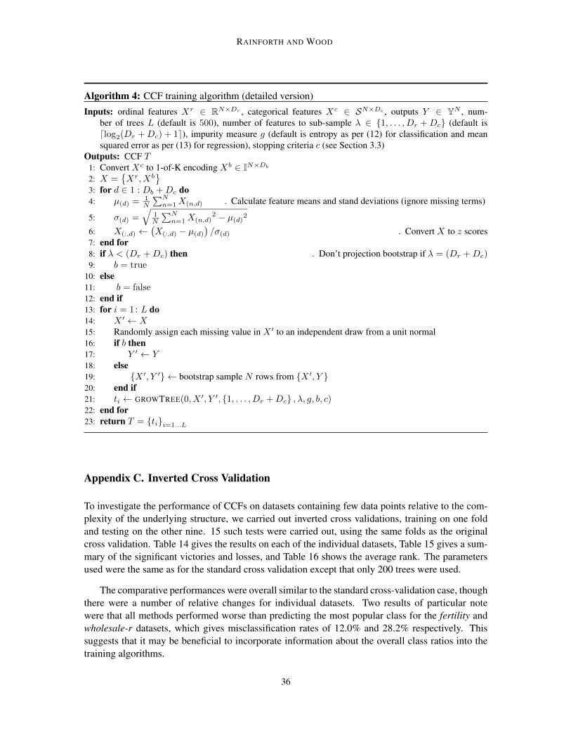
RAINFORTH AND WOOD

Algorithm 4: CCF training algorithm (detailed version)

Inputs: ordinal features Xr ∈ RN×Dr , categorical features Xc ∈ SN×Dc , outputs Y ∈ YN , num-ber of trees L (default is 500), number of features to sub-sample λ ∈ 1, . . . , Dr +Dc (default isdlog2(Dr +Dc) + 1e), impurity measure g (default is entropy as per (12) for classification and meansquared error as per (13) for regression), stopping criteria c (see Section 3.3)

Outputs: CCF T1: Convert Xc to 1-of-K encoding Xb ∈ IN×Db2: X =

Xr, Xb

3: for d ∈ 1 : Db +Dc do4: µ(d) = 1

N

∑Nn=1X(n,d) . Calculate feature means and stand deviations (ignore missing terms)

5: σ(d) =√

1N

∑Nn=1X(n,d)

2 − µ(d)2

6: X(:,d) ←(X(:,d) − µ(d)

)/σ(d) . Convert X to z scores

7: end for8: if λ < (Dr +Dc) then . Don’t projection bootstrap if λ = (Dr +Dc)9: b = true

10: else11: b = false12: end if13: for i = 1: L do14: X ′ ← X15: Randomly assign each missing value in X ′ to an independent draw from a unit normal16: if b then17: Y ′ ← Y18: else19: X ′, Y ′ ← bootstrap sample N rows from X ′, Y 20: end if21: ti ← GROWTREE(0, X ′, Y ′, 1, . . . , Dr +Dc , λ, g, b, c)22: end for23: return T = tii=1...L

Appendix C. Inverted Cross Validation

To investigate the performance of CCFs on datasets containing few data points relative to the com-plexity of the underlying structure, we carried out inverted cross validations, training on one foldand testing on the other nine. 15 such tests were carried out, using the same folds as the originalcross validation. Table 14 gives the results on each of the individual datasets, Table 15 gives a sum-mary of the significant victories and losses, and Table 16 shows the average rank. The parametersused were the same as for the standard cross validation except that only 200 trees were used.

The comparative performances were overall similar to the standard cross-validation case, thoughthere were a number of relative changes for individual datasets. Two results of particular notewere that all methods performed worse than predicting the most popular class for the fertility andwholesale-r datasets, which gives misclassification rates of 12.0% and 28.2% respectively. Thissuggests that it may be beneficial to incorporate information about the overall class ratios into thetraining algorithms.

36

CANONICAL CORRELATION FORESTS

Algorithm 5: GROWTREE (detailed version)

Inputs: unique node identifier for root node j, Xj = X(ωj ,:) ∈ RNj×(Dr+Db), Y j = Y(ωj ,:) ∈ YNj ,available feature ids Dj ⊆ 1, . . . , Dr +Dc, λ, g, whether to projection bootstrap b, c

Outputs: subtree Ψj ,Θj where Ψj are discriminant nodes and Θj leaf nodes1: Sample δj ⊆ Dj by taking min (λ, |Dj |) samples without replacement from Dj

2: While δj contains features without variation, eliminate these from Dj and δj and resample3: γj = δj mapped to the column indices of Xj in accordance with the 1-of-K encoding of Xc

4: if b then5: X ′,Y ′ ← bootstrap sample Nj data points from Xj

(:,γ), Yj

6: else7: X ′,Y ′ ←

Xj

(:,γ), Yj

8: end if9: if all rows in X ′ or Y ′ are identical then

10: if all rows in X j(:,γ) or Y j are identical then return·,j, 1Nj

∑Njn=1 Y

j(n,:)

end if

11: X ′,Y ′ ← Xj(:,γ), Y

j12: end if13: if X ′ contains only two unique rows then14: X = UNIQUEROWS(X ′)15: φj ← X(2,:) − X(1,:)

16: sj ← 12

(X(1,:) + X(2,:)

)φj

17: else18: Φ,Ω ← CCA(X ′,Y ′) . Calculate CCA coefficients using bootstrap sample19: U ← XΦ . Project original features into canonical component space20: Gbase ← g

(Y j)

21: for ν ∈ 1 : νmax do . νmax = min (rank (X ′) , rank (Y ′)) is number of canonical coefficient pairs22: u← SORT(U(:,ν))23: for i ∈ 2 : Nj do . Exhaustive search on unique splits24: S(i,ν) ← (u(i−1) + u(i))/2 . Split halfway between consecutive points.25: τ ` ←

n ∈ 1, . . . , Nj : U(n,ν) ≤ S(i,ν)

26: Nχj,` ← number of elements in τ `

27: τ r ← 1, . . . , Nj \τ `

28: G(i,ν) ← Gbase −Nχj,`Nj

g(Y(τ`,:)

)− Nj−Nχj,`

Njg(Y(τr,:)

). Split gain

29: end for . In practise gain is calculated by iterating from previous value to avoid N2j complexity.

30: end for31: i∗, ν∗ ← argmaxi,ν G(i,ν) . Choose best split32: if G(i∗,ν∗) ≤ 0 or any of c satisfied then . Node is a leaf33: θj ← 1

Nj

∑Njn=1 Y

j(n,:)

34: return ·, j, θj35: end if36: φj ← Φ(:,ν∗), sj ← S(i∗,ν∗) . Chosen projection and split point37: end if38: Generate unique identifiers for children χj,` and χj,r39: ψj ← j, δj , φj , sj , χj,`, χj,r40: τ ` ←

n ∈ 1, . . . , Nj : U(n,ν∗) ≤ S(i∗,ν∗)

, τ r ← 1, . . . , Nj \τ ` . Assign datapoints to children

41: Ψ`,Θ` ← GROWTREE(χj,`, Xj(τ`,:)

, Y j(τ`,:)

, Dj , λ, g, b, c) . Recurse for left child and right child

42: Ψr,Θr ← GROWTREE(χj,r, Xj(τr,:), Y

j(τr,:), Dj , λ, g, b, c)

43: return ψj ∪Ψ` ∪Ψr,Θ` ∪Θr

37

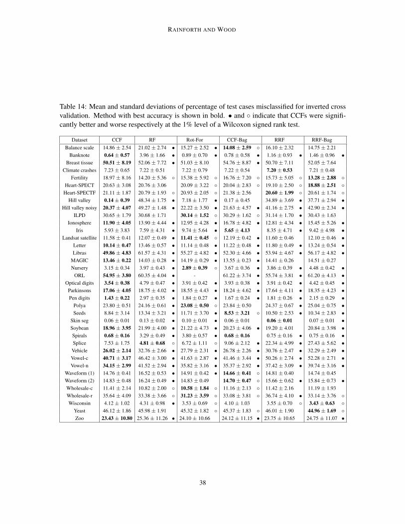
RAINFORTH AND WOOD

Table 14: Mean and standard deviations of percentage of test cases misclassified for inverted crossvalidation. Method with best accuracy is shown in bold. • and indicate that CCFs were signifi-cantly better and worse respectively at the 1% level of a Wilcoxon signed rank test.

Dataset CCF RF Rot-For CCF-Bag RRF RRF-BagBalance scale 14.86 ± 2.54 21.02 ± 2.74 • 15.27 ± 2.52 • 14.08 ± 2.59 16.10 ± 2.32 14.75 ± 2.21

Banknote 0.64 ± 0.57 3.96 ± 1.66 • 0.89 ± 0.70 • 0.78 ± 0.58 • 1.16 ± 0.93 • 1.46 ± 0.96 •Breast tissue 50.51 ± 8.19 52.06 ± 7.72 • 51.03 ± 8.10 54.76 ± 8.87 • 50.70 ± 7.11 52.05 ± 7.64

Climate crashes 7.23 ± 0.65 7.22 ± 0.51 7.22 ± 0.79 7.22 ± 0.54 7.20 ± 0.53 7.21 ± 0.48Fertility 18.97 ± 8.16 14.20 ± 5.36 15.38 ± 5.92 16.76 ± 7.20 15.73 ± 5.05 13.28 ± 2.88

Heart-SPECT 20.63 ± 3.08 20.76 ± 3.06 20.09 ± 3.22 20.04 ± 2.83 19.10 ± 2.50 18.88 ± 2.51 Heart-SPECTF 21.11 ± 1.87 20.79 ± 1.93 20.93 ± 2.05 21.38 ± 2.56 20.60 ± 1.99 20.61 ± 1.74

Hill valley 0.14 ± 0.39 48.34 ± 1.75 • 7.18 ± 1.77 • 0.17 ± 0.45 34.89 ± 3.69 • 37.71 ± 2.94 •Hill valley noisy 20.37 ± 4.07 49.27 ± 1.48 • 22.22 ± 3.50 • 21.63 ± 4.57 • 41.16 ± 2.75 • 42.90 ± 2.34 •

ILPD 30.65 ± 1.79 30.68 ± 1.71 30.14 ± 1.52 30.29 ± 1.62 31.14 ± 1.70 • 30.43 ± 1.63Ionosphere 11.90 ± 4.05 13.90 ± 4.44 • 12.95 ± 4.28 • 16.78 ± 4.82 • 12.81 ± 4.34 • 15.45 ± 5.26 •

Iris 5.93 ± 3.83 7.59 ± 4.31 • 9.74 ± 5.64 • 5.65 ± 4.13 8.35 ± 4.71 • 9.42 ± 4.98 •Landsat satellite 11.58 ± 0.41 12.07 ± 0.49 • 11.41 ± 0.45 12.19 ± 0.42 • 11.60 ± 0.46 12.10 ± 0.46 •

Letter 10.14 ± 0.47 13.46 ± 0.57 • 11.14 ± 0.48 • 11.22 ± 0.48 • 11.80 ± 0.49 • 13.24 ± 0.54 •Libras 49.86 ± 4.83 61.57 ± 4.31 • 55.27 ± 4.82 • 52.30 ± 4.66 • 53.94 ± 4.67 • 56.17 ± 4.82 •

MAGIC 13.46 ± 0.22 14.03 ± 0.28 • 14.19 ± 0.29 • 13.55 ± 0.23 • 14.41 ± 0.26 14.51 ± 0.27Nursery 3.15 ± 0.34 3.97 ± 0.43 • 2.89 ± 0.39 3.67 ± 0.36 • 3.86 ± 0.39 • 4.48 ± 0.42 •

ORL 54.95 ± 3.80 60.35 ± 4.04 • - 61.22 ± 3.74 • 55.74 ± 3.81 • 61.20 ± 4.13 •Optical digits 3.54 ± 0.38 4.79 ± 0.47 • 3.91 ± 0.42 • 3.93 ± 0.38 • 3.91 ± 0.42 • 4.42 ± 0.45 •

Parkinsons 17.06 ± 4.05 18.75 ± 4.02 • 18.55 ± 4.43 • 18.24 ± 4.62 • 17.64 ± 4.11 • 18.35 ± 4.23 •Pen digits 1.43 ± 0.22 2.97 ± 0.35 • 1.84 ± 0.27 • 1.67 ± 0.24 • 1.81 ± 0.26 • 2.15 ± 0.29 •

Polya 23.80 ± 0.51 24.16 ± 0.61 • 23.08 ± 0.50 23.84 ± 0.50 24.37 ± 0.67 • 25.04 ± 0.75 •Seeds 8.84 ± 3.14 13.34 ± 3.21 • 11.71 ± 3.70 • 8.53 ± 3.21 10.50 ± 2.53 • 10.34 ± 2.83 •

Skin seg 0.06 ± 0.01 0.13 ± 0.02 • 0.10 ± 0.01 • 0.06 ± 0.01 0.06 ± 0.01 0.07 ± 0.01 •Soybean 18.96 ± 3.95 21.99 ± 4.00 • 21.22 ± 4.73 • 20.23 ± 4.06 • 19.20 ± 4.01 20.84 ± 3.98 •Spirals 0.68 ± 0.16 3.29 ± 0.49 • 3.80 ± 0.57 • 0.68 ± 0.16 0.75 ± 0.16 • 0.75 ± 0.16 •Splice 7.53 ± 1.75 4.81 ± 0.68 6.72 ± 1.11 9.06 ± 2.12 • 22.34 ± 4.99 • 27.43 ± 5.62 •Vehicle 26.02 ± 2.14 32.76 ± 2.66 • 27.79 ± 2.31 • 26.78 ± 2.26 • 30.76 ± 2.47 • 32.29 ± 2.49 •Vowel-c 40.71 ± 3.17 46.42 ± 3.00 • 41.63 ± 2.87 • 41.46 ± 3.44 • 50.26 ± 2.74 • 52.28 ± 2.71 •Vowel-n 34.15 ± 2.99 41.52 ± 2.94 • 35.82 ± 3.16 • 35.37 ± 2.92 • 37.42 ± 3.09 • 39.74 ± 3.16 •

Waveform (1) 14.76 ± 0.41 16.52 ± 0.53 • 14.91 ± 0.42 • 14.66 ± 0.41 14.81 ± 0.40 14.74 ± 0.45Waveform (2) 14.83 ± 0.48 16.24 ± 0.49 • 14.83 ± 0.49 14.70 ± 0.47 15.66 ± 0.62 • 15.84 ± 0.73 •Wholesale-c 11.41 ± 2.14 10.82 ± 2.00 10.58 ± 1.84 11.16 ± 2.13 11.42 ± 2.16 11.19 ± 1.93Wholesale-r 35.64 ± 4.09 33.38 ± 3.66 31.23 ± 3.59 33.08 ± 3.81 36.74 ± 4.10 • 33.14 ± 3.76 Wisconsin 4.12 ± 1.02 4.31 ± 0.98 • 3.53 ± 0.69 4.10 ± 1.03 3.55 ± 0.70 3.43 ± 0.63

Yeast 46.12 ± 1.86 45.98 ± 1.91 45.32 ± 1.82 45.37 ± 1.83 46.01 ± 1.90 44.96 ± 1.69 Zoo 23.43 ± 10.80 25.36 ± 11.26 • 24.10 ± 10.66 24.12 ± 11.15 • 23.75 ± 10.65 24.75 ± 11.07 •

38

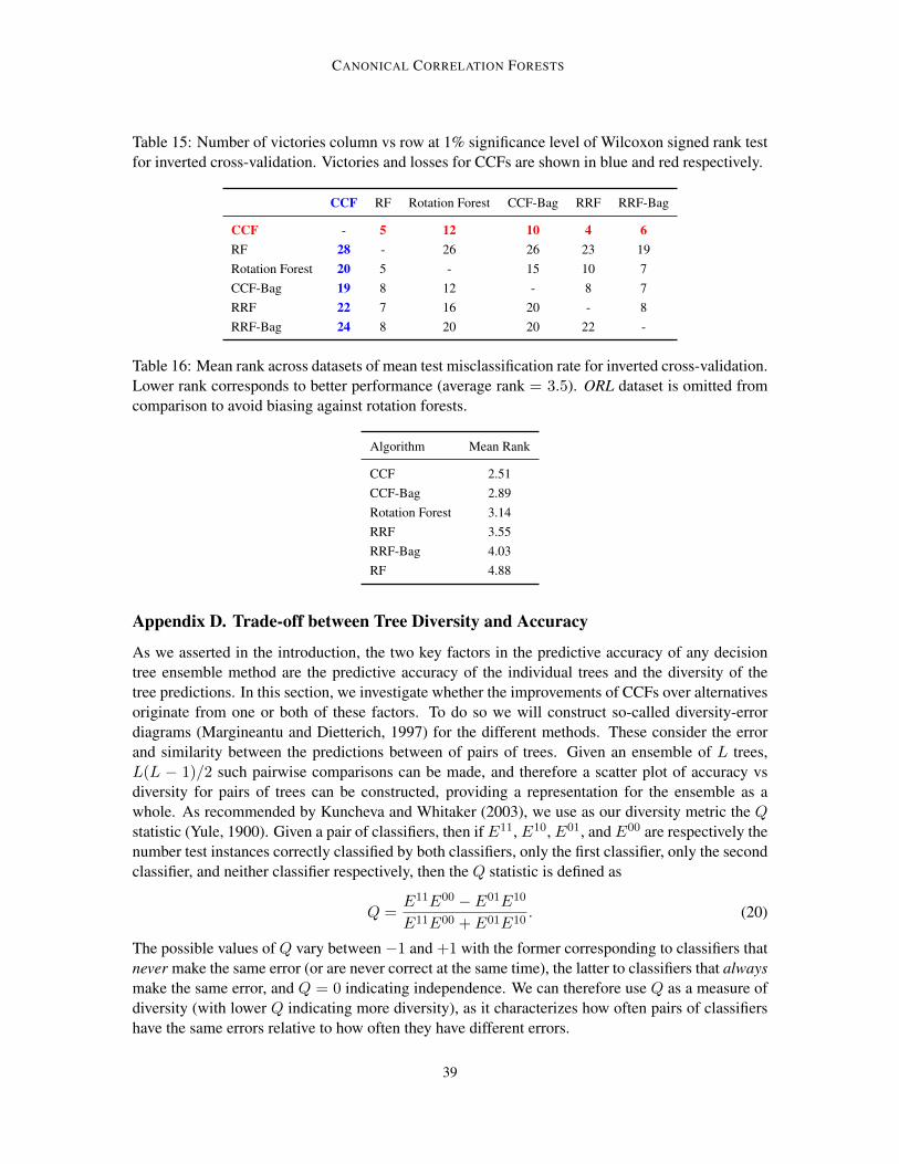
CANONICAL CORRELATION FORESTS

Table 15: Number of victories column vs row at 1% significance level of Wilcoxon signed rank testfor inverted cross-validation. Victories and losses for CCFs are shown in blue and red respectively.

CCF RF Rotation Forest CCF-Bag RRF RRF-Bag

CCF - 5 12 10 4 6RF 28 - 26 26 23 19Rotation Forest 20 5 - 15 10 7CCF-Bag 19 8 12 - 8 7RRF 22 7 16 20 - 8RRF-Bag 24 8 20 20 22 -

Table 16: Mean rank across datasets of mean test misclassification rate for inverted cross-validation.Lower rank corresponds to better performance (average rank = 3.5). ORL dataset is omitted fromcomparison to avoid biasing against rotation forests.

Algorithm Mean Rank

CCF 2.51CCF-Bag 2.89Rotation Forest 3.14RRF 3.55RRF-Bag 4.03RF 4.88

Appendix D. Trade-off between Tree Diversity and Accuracy

As we asserted in the introduction, the two key factors in the predictive accuracy of any decisiontree ensemble method are the predictive accuracy of the individual trees and the diversity of thetree predictions. In this section, we investigate whether the improvements of CCFs over alternativesoriginate from one or both of these factors. To do so we will construct so-called diversity-errordiagrams (Margineantu and Dietterich, 1997) for the different methods. These consider the errorand similarity between the predictions between of pairs of trees. Given an ensemble of L trees,L(L − 1)/2 such pairwise comparisons can be made, and therefore a scatter plot of accuracy vsdiversity for pairs of trees can be constructed, providing a representation for the ensemble as awhole. As recommended by Kuncheva and Whitaker (2003), we use as our diversity metric the Qstatistic (Yule, 1900). Given a pair of classifiers, then if E11, E10, E01, and E00 are respectively thenumber test instances correctly classified by both classifiers, only the first classifier, only the secondclassifier, and neither classifier respectively, then the Q statistic is defined as

Q =E11E00 − E01E10

E11E00 + E01E10. (20)

The possible values of Q vary between −1 and +1 with the former corresponding to classifiers thatnever make the same error (or are never correct at the same time), the latter to classifiers that alwaysmake the same error, and Q = 0 indicating independence. We can therefore use Q as a measure ofdiversity (with lower Q indicating more diversity), as it characterizes how often pairs of classifiershave the same errors relative to how often they have different errors.

39

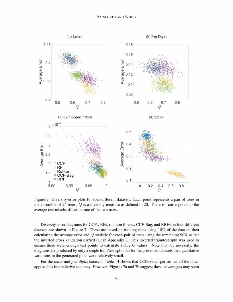
RAINFORTH AND WOOD

(a) Letter (b) Pen Digits

(c) Skin Segmentation (d) Splice

Figure 7: Diversity-error plots for four different datasets. Each point represents a pair of trees inthe ensemble of 25 trees. Q is a diversity measure as defined in 20. The error corresponds to theaverage test misclassification rate of the two trees.

Diversity-error diagrams for CCFs, RFs, rotation forests, CCF-Bag, and RRFs on four differentdatasets are shown in Figure 7. These are based on training trees using 10% of the data an thencalculating the average error and Q statistic for each pair of trees using the remaining 90% as perthe inverted cross validation carried out in Appendix C. This inverted train/test split was used toensure there were enough test points to calculate stable Q values. Note that, by necessity, thediagrams are produced by only a single train/test split, but for the presented datasets then qualitativevariations in the generated plots were relatively small.

For the letter and pen digits datasets, Table 14 shows that CCFs outer-performed all the otherapproaches in predictive accuracy. However, Figures 7a and 7b suggest these advantages may stem

40

CANONICAL CORRELATION FORESTS

from different causes. Figure 7b shows a similarly diversity for all the approaches on the pen digitsdataset, but a better tree accuracy for CCFs than the others. Figure 7a suggests that CCFs may haveoutperformed CCF-Bag and RRFs on the letter dataset due to having better individual tree accuracy,but the advantages compared with RFs now seem to stem from better diversity. Rotation forests hada better tree accuracy but worse diversity than CCFs, with the better ensemble performance of CCFssuggesting they had a better trade-off for this dataset.

For the skin segmentation dataset then Table 14 shows that CCFs outperformed RFs and rotationforests, but had similar performance to CCF-Bag and RRFs. Figure 7c suggests that the advantageover RFs comes from better tree accuracy and the advantage over rotation forests from better diver-sity. It shows that CCFs gave more accurate but less diverse trees than CCF-Bag and RRFs.

For the splice dataset then CCFs outperformed CCF-Bag and RRFs (with the latter doing par-ticularly poorly), but were outperformed by RFs and rotation forests. From Figure 7d, the poortree accuracy of RRFs is very apparent, while RFs seem to give better accuracy than CCFs, at theexpense of slightly less diversity. Rotation forests, which were outperformed by RFs, gave signifi-cantly more accurate trees than all the other approaches, but far less diversity.

Other than suggesting a tendency for rotation forests to produce relatively accurate but lowdiversity trees, the diagrams do not appear to show a clear pattern of differences. This suggests thatthe advantages of CCFs can originate from either improved tree accuracy or diversity depending onthe dataset.

Appendix E. Detailed Results for Comparisons to Other Classifiers

Table 17 gives a detailed comparison of CCFs to MATLAB’s TREEBAGGER algorithm, along witha comparison to a summary of the performance of the 179 classifiers tested in Fernandez-Delgadoet al. (2014) for 82 UCI datasets. Both CCFs and TREEBAGGER used 500 trees and the default treeparameter settings laid out in Section 3.3.3. For significance comparisons with the TREEBAGGER

algorithm a 10% significance level was necessary as the Wilcoxon signed rank test cannot give ap-value lower than 6.25% for 4-fold cross validation. This gave a win/draw/loss ratio for CCFs of22/56/4. It should be noted that the number of losses is no more than would be expected by chanceand that the reason that there are many more draws than in the tests of Section 3.1 is that a manyfewer tests were carried out for each dataset (4 instead of 150). There were a number of datasetswere CCFs performed noticeably better then any of the other classifiers, with the performance onthe hill-valley-noisy dataset particularly impressive, giving a error rate of 6.93% with the next bestclassifier only achieving 25.7%.

41

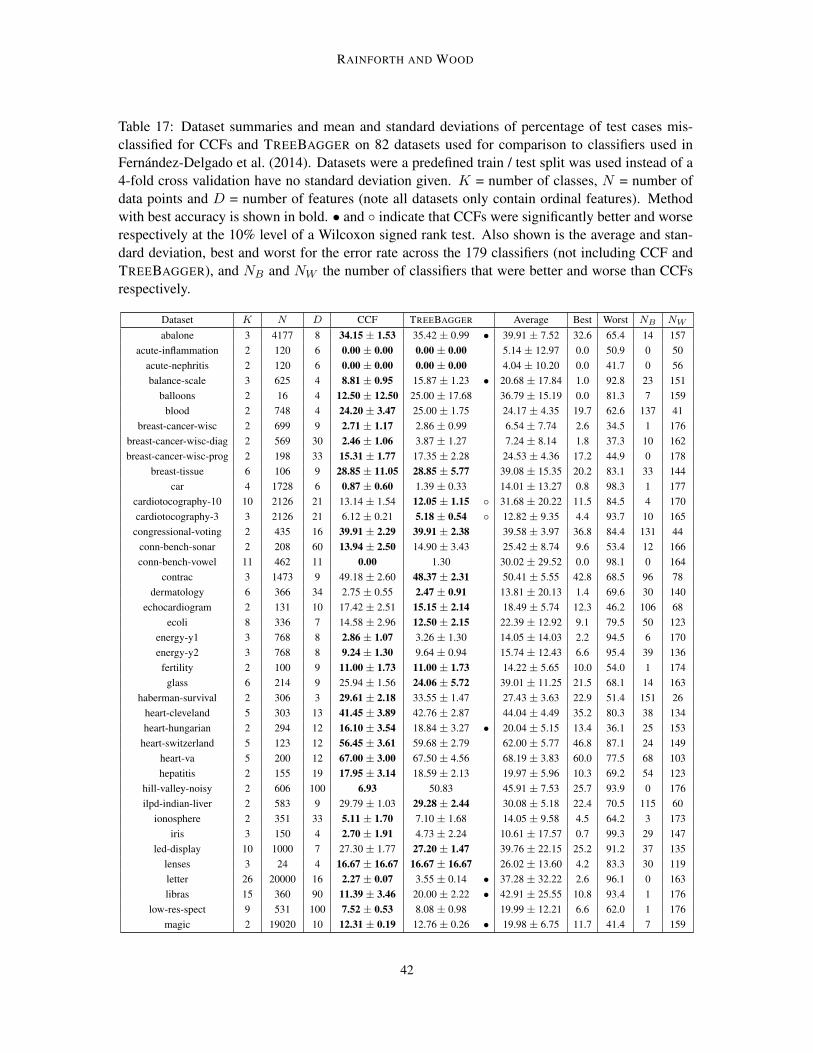
RAINFORTH AND WOOD

Table 17: Dataset summaries and mean and standard deviations of percentage of test cases mis-classified for CCFs and TREEBAGGER on 82 datasets used for comparison to classifiers used inFernandez-Delgado et al. (2014). Datasets were a predefined train / test split was used instead of a4-fold cross validation have no standard deviation given. K = number of classes, N = number ofdata points and D = number of features (note all datasets only contain ordinal features). Methodwith best accuracy is shown in bold. • and indicate that CCFs were significantly better and worserespectively at the 10% level of a Wilcoxon signed rank test. Also shown is the average and stan-dard deviation, best and worst for the error rate across the 179 classifiers (not including CCF andTREEBAGGER), and NB and NW the number of classifiers that were better and worse than CCFsrespectively.

Dataset K N D CCF TREEBAGGER Average Best Worst NB NW

abalone 3 4177 8 34.15 ± 1.53 35.42 ± 0.99 • 39.91 ± 7.52 32.6 65.4 14 157acute-inflammation 2 120 6 0.00 ± 0.00 0.00 ± 0.00 5.14 ± 12.97 0.0 50.9 0 50

acute-nephritis 2 120 6 0.00 ± 0.00 0.00 ± 0.00 4.04 ± 10.20 0.0 41.7 0 56balance-scale 3 625 4 8.81 ± 0.95 15.87 ± 1.23 • 20.68 ± 17.84 1.0 92.8 23 151

balloons 2 16 4 12.50 ± 12.50 25.00 ± 17.68 36.79 ± 15.19 0.0 81.3 7 159blood 2 748 4 24.20 ± 3.47 25.00 ± 1.75 24.17 ± 4.35 19.7 62.6 137 41

breast-cancer-wisc 2 699 9 2.71 ± 1.17 2.86 ± 0.99 6.54 ± 7.74 2.6 34.5 1 176breast-cancer-wisc-diag 2 569 30 2.46 ± 1.06 3.87 ± 1.27 7.24 ± 8.14 1.8 37.3 10 162breast-cancer-wisc-prog 2 198 33 15.31 ± 1.77 17.35 ± 2.28 24.53 ± 4.36 17.2 44.9 0 178

breast-tissue 6 106 9 28.85 ± 11.05 28.85 ± 5.77 39.08 ± 15.35 20.2 83.1 33 144car 4 1728 6 0.87 ± 0.60 1.39 ± 0.33 14.01 ± 13.27 0.8 98.3 1 177

cardiotocography-10 10 2126 21 13.14 ± 1.54 12.05 ± 1.15 31.68 ± 20.22 11.5 84.5 4 170cardiotocography-3 3 2126 21 6.12 ± 0.21 5.18 ± 0.54 12.82 ± 9.35 4.4 93.7 10 165

congressional-voting 2 435 16 39.91 ± 2.29 39.91 ± 2.38 39.58 ± 3.97 36.8 84.4 131 44conn-bench-sonar 2 208 60 13.94 ± 2.50 14.90 ± 3.43 25.42 ± 8.74 9.6 53.4 12 166conn-bench-vowel 11 462 11 0.00 1.30 30.02 ± 29.52 0.0 98.1 0 164

contrac 3 1473 9 49.18 ± 2.60 48.37 ± 2.31 50.41 ± 5.55 42.8 68.5 96 78dermatology 6 366 34 2.75 ± 0.55 2.47 ± 0.91 13.81 ± 20.13 1.4 69.6 30 140

echocardiogram 2 131 10 17.42 ± 2.51 15.15 ± 2.14 18.49 ± 5.74 12.3 46.2 106 68ecoli 8 336 7 14.58 ± 2.96 12.50 ± 2.15 22.39 ± 12.92 9.1 79.5 50 123

energy-y1 3 768 8 2.86 ± 1.07 3.26 ± 1.30 14.05 ± 14.03 2.2 94.5 6 170energy-y2 3 768 8 9.24 ± 1.30 9.64 ± 0.94 15.74 ± 12.43 6.6 95.4 39 136

fertility 2 100 9 11.00 ± 1.73 11.00 ± 1.73 14.22 ± 5.65 10.0 54.0 1 174glass 6 214 9 25.94 ± 1.56 24.06 ± 5.72 39.01 ± 11.25 21.5 68.1 14 163

haberman-survival 2 306 3 29.61 ± 2.18 33.55 ± 1.47 27.43 ± 3.63 22.9 51.4 151 26heart-cleveland 5 303 13 41.45 ± 3.89 42.76 ± 2.87 44.04 ± 4.49 35.2 80.3 38 134heart-hungarian 2 294 12 16.10 ± 3.54 18.84 ± 3.27 • 20.04 ± 5.15 13.4 36.1 25 153

heart-switzerland 5 123 12 56.45 ± 3.61 59.68 ± 2.79 62.00 ± 5.77 46.8 87.1 24 149heart-va 5 200 12 67.00 ± 3.00 67.50 ± 4.56 68.19 ± 3.83 60.0 77.5 68 103hepatitis 2 155 19 17.95 ± 3.14 18.59 ± 2.13 19.97 ± 5.96 10.3 69.2 54 123

hill-valley-noisy 2 606 100 6.93 50.83 45.91 ± 7.53 25.7 93.9 0 176ilpd-indian-liver 2 583 9 29.79 ± 1.03 29.28 ± 2.44 30.08 ± 5.18 22.4 70.5 115 60

ionosphere 2 351 33 5.11 ± 1.70 7.10 ± 1.68 14.05 ± 9.58 4.5 64.2 3 173iris 3 150 4 2.70 ± 1.91 4.73 ± 2.24 10.61 ± 17.57 0.7 99.3 29 147

led-display 10 1000 7 27.30 ± 1.77 27.20 ± 1.47 39.76 ± 22.15 25.2 91.2 37 135lenses 3 24 4 16.67 ± 16.67 16.67 ± 16.67 26.02 ± 13.60 4.2 83.3 30 119letter 26 20000 16 2.27 ± 0.07 3.55 ± 0.14 • 37.28 ± 32.22 2.6 96.1 0 163libras 15 360 90 11.39 ± 3.46 20.00 ± 2.22 • 42.91 ± 25.55 10.8 93.4 1 176

low-res-spect 9 531 100 7.52 ± 0.53 8.08 ± 0.98 19.99 ± 12.21 6.6 62.0 1 176magic 2 19020 10 12.31 ± 0.19 12.76 ± 0.26 • 19.98 ± 6.75 11.7 41.4 7 159

42

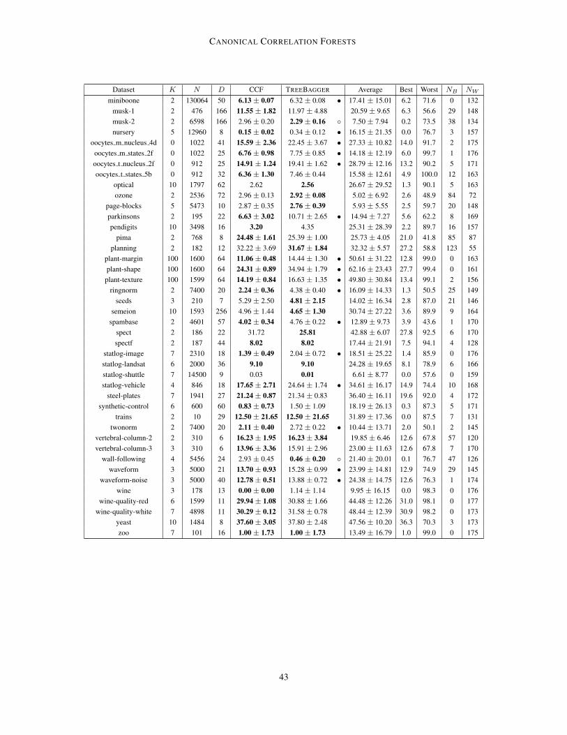
CANONICAL CORRELATION FORESTS

Dataset K N D CCF TREEBAGGER Average Best Worst NB NW

miniboone 2 130064 50 6.13 ± 0.07 6.32 ± 0.08 • 17.41 ± 15.01 6.2 71.6 0 132musk-1 2 476 166 11.55 ± 1.82 11.97 ± 4.88 20.59 ± 9.65 6.3 56.6 29 148musk-2 2 6598 166 2.96 ± 0.20 2.29 ± 0.16 7.50 ± 7.94 0.2 73.5 38 134nursery 5 12960 8 0.15 ± 0.02 0.34 ± 0.12 • 16.15 ± 21.35 0.0 76.7 3 157

oocytes m nucleus 4d 0 1022 41 15.59 ± 2.36 22.45 ± 3.67 • 27.33 ± 10.82 14.0 91.7 2 175oocytes m states 2f 0 1022 25 6.76 ± 0.98 7.75 ± 0.85 • 14.18 ± 12.19 6.0 99.7 1 176oocytes t nucleus 2f 0 912 25 14.91 ± 1.24 19.41 ± 1.62 • 28.79 ± 12.16 13.2 90.2 5 171oocytes t states 5b 0 912 32 6.36 ± 1.30 7.46 ± 0.44 15.58 ± 12.61 4.9 100.0 12 163

optical 10 1797 62 2.62 2.56 26.67 ± 29.52 1.3 90.1 5 163ozone 2 2536 72 2.96 ± 0.13 2.92 ± 0.08 5.02 ± 6.92 2.6 48.9 84 72

page-blocks 5 5473 10 2.87 ± 0.35 2.76 ± 0.39 5.93 ± 5.55 2.5 59.7 20 148parkinsons 2 195 22 6.63 ± 3.02 10.71 ± 2.65 • 14.94 ± 7.27 5.6 62.2 8 169pendigits 10 3498 16 3.20 4.35 25.31 ± 28.39 2.2 89.7 16 157

pima 2 768 8 24.48 ± 1.61 25.39 ± 1.00 25.73 ± 4.05 21.0 41.8 85 87planning 2 182 12 32.22 ± 3.69 31.67 ± 1.84 32.32 ± 5.57 27.2 58.8 123 55

plant-margin 100 1600 64 11.06 ± 0.48 14.44 ± 1.30 • 50.61 ± 31.22 12.8 99.0 0 163plant-shape 100 1600 64 24.31 ± 0.89 34.94 ± 1.79 • 62.16 ± 23.43 27.7 99.4 0 161plant-texture 100 1599 64 14.19 ± 0.84 16.63 ± 1.35 • 49.80 ± 30.84 13.4 99.1 2 156

ringnorm 2 7400 20 2.24 ± 0.36 4.38 ± 0.40 • 16.09 ± 14.33 1.3 50.5 25 149seeds 3 210 7 5.29 ± 2.50 4.81 ± 2.15 14.02 ± 16.34 2.8 87.0 21 146

semeion 10 1593 256 4.96 ± 1.44 4.65 ± 1.30 30.74 ± 27.22 3.6 89.9 9 164spambase 2 4601 57 4.02 ± 0.34 4.76 ± 0.22 • 12.89 ± 9.73 3.9 43.6 1 170

spect 2 186 22 31.72 25.81 42.88 ± 6.07 27.8 92.5 6 170spectf 2 187 44 8.02 8.02 17.44 ± 21.91 7.5 94.1 4 128

statlog-image 7 2310 18 1.39 ± 0.49 2.04 ± 0.72 • 18.51 ± 25.22 1.4 85.9 0 176statlog-landsat 6 2000 36 9.10 9.10 24.28 ± 19.65 8.1 78.9 6 166statlog-shuttle 7 14500 9 0.03 0.01 6.61 ± 8.77 0.0 57.6 0 159statlog-vehicle 4 846 18 17.65 ± 2.71 24.64 ± 1.74 • 34.61 ± 16.17 14.9 74.4 10 168

steel-plates 7 1941 27 21.24 ± 0.87 21.34 ± 0.83 36.40 ± 16.11 19.6 92.0 4 172synthetic-control 6 600 60 0.83 ± 0.73 1.50 ± 1.09 18.19 ± 26.13 0.3 87.3 5 171

trains 2 10 29 12.50 ± 21.65 12.50 ± 21.65 31.89 ± 17.36 0.0 87.5 7 131twonorm 2 7400 20 2.11 ± 0.40 2.72 ± 0.22 • 10.44 ± 13.71 2.0 50.1 2 145

vertebral-column-2 2 310 6 16.23 ± 1.95 16.23 ± 3.84 19.85 ± 6.46 12.6 67.8 57 120vertebral-column-3 3 310 6 13.96 ± 3.36 15.91 ± 2.96 23.00 ± 11.63 12.6 67.8 7 170

wall-following 4 5456 24 2.93 ± 0.45 0.46 ± 0.20 21.40 ± 20.01 0.1 76.7 47 126waveform 3 5000 21 13.70 ± 0.93 15.28 ± 0.99 • 23.99 ± 14.81 12.9 74.9 29 145

waveform-noise 3 5000 40 12.78 ± 0.51 13.88 ± 0.72 • 24.38 ± 14.75 12.6 76.3 1 174wine 3 178 13 0.00 ± 0.00 1.14 ± 1.14 9.95 ± 16.15 0.0 98.3 0 176

wine-quality-red 6 1599 11 29.94 ± 1.08 30.88 ± 1.66 44.48 ± 12.26 31.0 98.1 0 177wine-quality-white 7 4898 11 30.29 ± 0.12 31.58 ± 0.78 48.44 ± 12.39 30.9 98.2 0 173

yeast 10 1484 8 37.60 ± 3.05 37.80 ± 2.48 47.56 ± 10.20 36.3 70.3 3 173zoo 7 101 16 1.00 ± 1.73 1.00 ± 1.73 13.49 ± 16.79 1.0 99.0 0 175

43

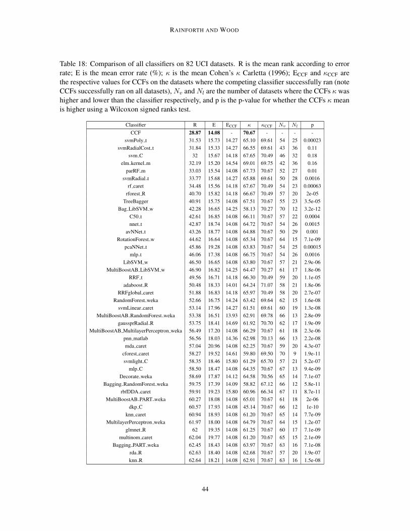
RAINFORTH AND WOOD

Table 18: Comparison of all classifiers on 82 UCI datasets. R is the mean rank according to errorrate; E is the mean error rate (%); κ is the mean Cohen’s κ Carletta (1996); ECCF and κCCF arethe respective values for CCFs on the datasets where the competing classifier successfully ran (noteCCFs successfully ran on all datasets), Nv andNl are the number of datasets where the CCFs κ washigher and lower than the classifier respectively, and p is the p-value for whether the CCFs κ meanis higher using a Wilcoxon signed ranks test.

Classifier R E ECCF κ κCCF Nv Nl pCCF 28.87 14.08 - 70.67 - - - -

svmPoly t 31.53 15.73 14.27 65.10 69.61 54 25 0.00023svmRadialCost t 31.84 15.33 14.27 66.55 69.61 43 36 0.11

svm C 32 15.67 14.18 67.65 70.49 46 32 0.18elm kernel m 32.19 15.20 14.54 69.01 69.75 42 36 0.16

parRF m 33.03 15.54 14.08 67.73 70.67 52 27 0.01svmRadial t 33.77 15.68 14.27 65.88 69.61 50 28 0.0016

rf caret 34.48 15.56 14.18 67.67 70.49 54 23 0.00063rforest R 40.70 15.82 14.18 66.67 70.49 57 20 2e-05

TreeBagger 40.91 15.75 14.08 67.51 70.67 55 23 3.5e-05Bag LibSVM w 42.28 16.65 14.25 58.13 70.27 70 12 3.2e-12

C50 t 42.61 16.85 14.08 66.11 70.67 57 22 0.0004nnet t 42.87 18.74 14.08 64.72 70.67 54 26 0.0015

avNNet t 43.26 18.77 14.08 64.88 70.67 50 29 0.001RotationForest w 44.62 16.64 14.08 65.34 70.67 64 15 7.1e-09

pcaNNet t 45.86 19.28 14.08 63.83 70.67 54 25 0.00015mlp t 46.06 17.38 14.08 66.75 70.67 54 26 0.0016

LibSVM w 46.50 16.65 14.08 63.80 70.67 57 21 2.9e-06MultiBoostAB LibSVM w 46.90 16.82 14.25 64.47 70.27 61 17 1.8e-06

RRF t 49.56 16.71 14.18 66.30 70.49 59 20 1.1e-05adaboost R 50.48 18.33 14.01 64.24 71.07 58 21 1.8e-06

RRFglobal caret 51.88 16.83 14.18 65.97 70.49 58 20 2.7e-07RandomForest weka 52.66 16.75 14.24 63.42 69.64 62 15 1.6e-08

svmLinear caret 53.14 17.96 14.27 61.51 69.61 60 19 1.3e-08MultiBoostAB RandomForest weka 53.38 16.51 13.93 62.91 69.78 66 13 2.8e-09

gaussprRadial R 53.75 18.41 14.69 61.92 70.70 62 17 1.9e-09MultiBoostAB MultilayerPerceptron weka 56.49 17.20 14.08 66.29 70.67 61 18 2.3e-06

pnn matlab 56.56 18.03 14.36 62.98 70.13 66 13 2.2e-08mda caret 57.04 20.96 14.08 62.25 70.67 59 20 4.3e-07

cforest caret 58.27 19.52 14.61 59.80 69.50 70 9 1.9e-11svmlight C 58.35 18.46 15.80 61.29 65.70 57 21 5.2e-07

mlp C 58.50 18.47 14.08 64.35 70.67 67 13 9.4e-09Decorate weka 58.69 17.87 14.12 64.58 70.56 65 14 7.1e-07

Bagging RandomForest weka 59.75 17.39 14.09 58.82 67.12 66 12 5.8e-11rbfDDA caret 59.91 19.23 15.80 60.96 66.34 67 11 8.7e-11

MultiBoostAB PART weka 60.27 18.08 14.08 65.01 70.67 61 18 2e-06dkp C 60.57 17.93 14.08 45.14 70.67 66 12 1e-10

knn caret 60.94 18.93 14.08 61.20 70.67 65 14 7.7e-09MultilayerPerceptron weka 61.97 18.00 14.08 64.79 70.67 64 15 1.2e-07

glmnet R 62 19.35 14.08 61.25 70.67 60 17 7.1e-09multinom caret 62.04 19.77 14.08 61.20 70.67 65 15 2.1e-09

Bagging PART weka 62.45 18.43 14.08 63.97 70.67 63 16 7.1e-08rda R 62.63 18.40 14.08 62.68 70.67 57 20 1.9e-07knn R 62.64 18.21 14.08 62.91 70.67 63 16 1.5e-08

44

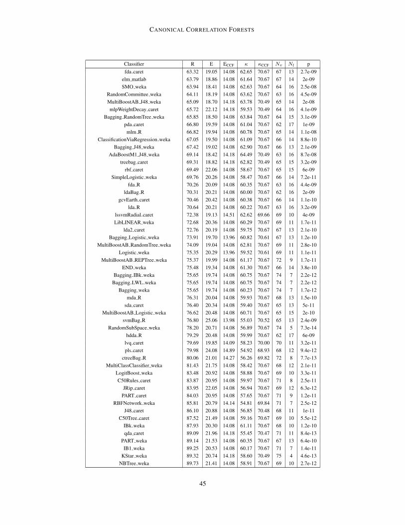
CANONICAL CORRELATION FORESTS

Classifier R E ECCF κ κCCF Nv Nl pfda caret 63.32 19.05 14.08 62.65 70.67 67 13 2.7e-09

elm matlab 63.79 18.86 14.08 61.64 70.67 67 14 2e-09SMO weka 63.94 18.41 14.08 62.63 70.67 64 16 2.5e-08

RandomCommittee weka 64.11 18.19 14.08 63.62 70.67 63 16 4.5e-09MultiBoostAB J48 weka 65.09 18.70 14.18 63.78 70.49 65 14 2e-08mlpWeightDecay caret 65.72 22.12 14.18 59.53 70.49 64 16 4.1e-09

Bagging RandomTree weka 65.85 18.50 14.08 63.84 70.67 64 15 3.1e-09pda caret 66.80 19.59 14.08 61.04 70.67 62 17 1e-09mlm R 66.82 19.94 14.08 60.78 70.67 65 14 1.1e-08

ClassificationViaRegression weka 67.05 19.50 14.08 61.09 70.67 66 14 8.8e-10Bagging J48 weka 67.42 19.02 14.08 62.90 70.67 66 13 2.1e-09

AdaBoostM1 J48 weka 69.14 18.42 14.18 64.49 70.49 63 16 8.7e-08treebag caret 69.31 18.82 14.18 62.82 70.49 65 15 3.2e-09

rbf caret 69.49 22.06 14.08 58.67 70.67 65 15 6e-09SimpleLogistic weka 69.76 20.26 14.08 58.47 70.67 66 14 7.2e-11

fda R 70.26 20.09 14.08 60.35 70.67 63 16 4.4e-09ldaBag R 70.31 20.21 14.08 60.00 70.67 62 16 2e-09

gcvEarth caret 70.46 20.42 14.08 60.38 70.67 66 14 1.1e-10lda R 70.64 20.21 14.08 60.22 70.67 63 16 3.2e-09

lssvmRadial caret 72.38 19.13 14.51 62.62 69.66 69 10 4e-09LibLINEAR weka 72.68 20.36 14.08 60.29 70.67 69 11 1.7e-11

lda2 caret 72.76 20.19 14.08 59.75 70.67 67 13 2.1e-10Bagging Logistic weka 73.91 19.70 13.96 60.82 70.61 67 13 1.2e-10

MultiBoostAB RandomTree weka 74.09 19.04 14.08 62.81 70.67 69 11 2.8e-10Logistic weka 75.35 20.29 13.96 59.52 70.61 69 11 1.1e-11

MultiBoostAB REPTree weka 75.37 19.99 14.08 61.17 70.67 72 9 1.7e-11END weka 75.48 19.34 14.08 61.30 70.67 66 14 3.8e-10

Bagging IBk weka 75.65 19.74 14.08 60.75 70.67 74 7 2.2e-12Bagging LWL weka 75.65 19.74 14.08 60.75 70.67 74 7 2.2e-12

Bagging weka 75.65 19.74 14.08 60.23 70.67 74 7 1.7e-12mda R 76.31 20.04 14.08 59.93 70.67 68 13 1.5e-10

sda caret 76.40 20.34 14.08 59.40 70.67 65 13 5e-11MultiBoostAB Logistic weka 76.62 20.48 14.08 60.71 70.67 65 15 2e-10

svmBag R 76.80 25.06 13.98 55.03 70.52 65 13 2.4e-09RandomSubSpace weka 78.20 20.71 14.08 56.89 70.67 74 5 7.3e-14

hdda R 79.29 20.48 14.08 59.99 70.67 62 17 6e-09lvq caret 79.69 19.85 14.09 58.23 70.00 70 11 3.2e-11pls caret 79.98 24.08 14.89 54.92 68.93 68 12 9.4e-12

ctreeBag R 80.06 21.01 14.27 56.26 69.82 72 8 7.7e-13MultiClassClassifier weka 81.43 21.75 14.08 58.42 70.67 68 12 2.1e-11

LogitBoost weka 83.48 20.92 14.08 58.88 70.67 69 10 3.3e-11C50Rules caret 83.87 20.95 14.08 59.97 70.67 71 8 2.5e-11

JRip caret 83.95 22.05 14.08 56.94 70.67 69 12 6.3e-12PART caret 84.03 20.95 14.08 57.65 70.67 71 9 1.2e-11

RBFNetwork weka 85.81 20.79 14.14 54.81 69.84 71 7 2.5e-12J48 caret 86.10 20.88 14.08 56.85 70.48 68 11 1e-11

C50Tree caret 87.52 21.49 14.08 59.16 70.67 69 10 5.5e-12IBk weka 87.93 20.30 14.08 61.11 70.67 68 10 1.2e-10qda caret 89.09 21.96 14.18 55.45 70.47 71 11 8.4e-13

PART weka 89.14 21.53 14.08 60.35 70.67 67 13 6.4e-10IB1 weka 89.25 20.53 14.08 60.17 70.67 71 7 1.4e-11

KStar weka 89.32 20.74 14.18 58.60 70.49 75 4 4.6e-13NBTree weka 89.73 21.41 14.08 58.91 70.67 69 10 2.7e-12

45

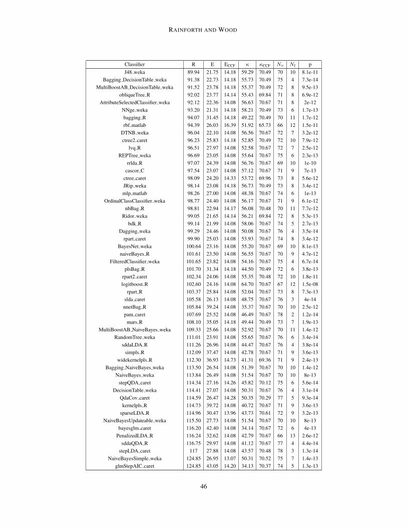
RAINFORTH AND WOOD

Classifier R E ECCF κ κCCF Nv Nl pJ48 weka 89.94 21.75 14.18 59.29 70.49 70 10 8.1e-11

Bagging DecisionTable weka 91.38 22.73 14.18 55.73 70.49 75 4 7.3e-14MultiBoostAB DecisionTable weka 91.52 23.78 14.18 55.37 70.49 72 8 9.5e-13

obliqueTree R 92.02 23.77 14.14 55.43 69.84 71 8 6.9e-12AttributeSelectedClassifier weka 92.12 22.36 14.08 56.63 70.67 71 8 2e-12

NNge weka 93.20 21.31 14.18 58.21 70.49 73 6 1.7e-13bagging R 94.07 31.45 14.18 49.22 70.49 70 11 1.7e-12rbf matlab 94.39 26.03 16.39 51.92 65.73 66 12 1.5e-11

DTNB weka 96.04 22.10 14.08 56.56 70.67 72 7 3.2e-12ctree2 caret 96.23 25.83 14.18 52.85 70.49 72 10 7.9e-12

lvq R 96.51 27.97 14.08 52.58 70.67 72 7 2.5e-12REPTree weka 96.69 23.05 14.08 55.64 70.67 75 6 2.3e-13

rrlda R 97.07 24.39 14.08 56.76 70.67 69 10 1e-10cascor C 97.54 23.07 14.08 57.12 70.67 71 9 7e-13

ctree caret 98.09 24.20 14.33 53.72 69.96 73 8 5.6e-12JRip weka 98.14 23.08 14.18 56.73 70.49 73 8 3.4e-12mlp matlab 98.26 27.00 14.08 48.38 70.67 74 6 1e-13

OrdinalClassClassifier weka 98.77 24.40 14.08 56.17 70.67 71 9 6.1e-12nbBag R 98.81 22.94 14.17 56.08 70.48 70 11 7.7e-12

Ridor weka 99.05 21.65 14.14 56.21 69.84 72 8 5.3e-13bdk R 99.14 21.99 14.08 58.06 70.67 74 5 2.7e-13

Dagging weka 99.29 24.46 14.08 50.08 70.67 76 4 3.5e-14rpart caret 99.90 25.03 14.08 53.93 70.67 74 8 3.4e-12

BayesNet weka 100.64 23.16 14.08 55.20 70.67 69 10 8.1e-13naiveBayes R 101.61 23.50 14.08 56.55 70.67 70 9 4.7e-12

FilteredClassifier weka 101.65 23.82 14.08 54.16 70.67 75 4 6.7e-14plsBag R 101.70 31.34 14.18 44.50 70.49 72 6 3.8e-13

rpart2 caret 102.34 24.06 14.08 55.35 70.48 72 10 1.8e-11logitboost R 102.60 24.16 14.08 64.70 70.67 67 12 1.5e-08

rpart R 103.37 25.84 14.08 52.04 70.67 73 8 7.3e-13slda caret 105.58 26.13 14.08 48.75 70.67 76 3 4e-14nnetBag R 105.84 39.24 14.08 35.37 70.67 70 10 2.5e-12pam caret 107.69 25.52 14.08 46.49 70.67 78 2 1.2e-14

mars R 108.10 35.05 14.18 49.44 70.49 73 7 1.9e-13MultiBoostAB NaiveBayes weka 109.33 25.66 14.08 52.92 70.67 70 11 1.4e-12

RandomTree weka 111.01 23.91 14.08 55.65 70.67 76 6 3.4e-14sddaLDA R 111.26 26.96 14.08 44.47 70.67 76 4 3.8e-14

simpls R 112.09 37.47 14.08 42.78 70.67 71 9 3.6e-13widekernelpls R 112.30 36.93 14.73 41.31 69.36 71 9 2.4e-13

Bagging NaiveBayes weka 113.50 26.54 14.08 51.39 70.67 70 10 1.4e-12NaiveBayes weka 113.84 26.49 14.08 51.54 70.67 70 10 8e-13

stepQDA caret 114.34 27.16 14.26 45.82 70.12 75 6 5.6e-14DecisionTable weka 114.41 27.07 14.08 50.31 70.67 76 4 3.1e-14

QdaCov caret 114.59 26.47 14.28 50.35 70.29 77 5 9.3e-14kernelpls R 114.73 39.72 14.08 40.72 70.67 71 9 3.6e-13

sparseLDA R 114.96 30.47 13.96 43.73 70.61 72 9 3.2e-13NaiveBayesUpdateable weka 115.50 27.73 14.08 51.54 70.67 70 10 8e-13

bayesglm caret 116.20 42.40 14.08 34.14 70.67 72 6 4e-13PenalizedLDA R 116.24 32.62 14.08 42.79 70.67 66 13 2.6e-12

sddaQDA R 116.75 29.97 14.08 41.12 70.67 77 4 4.4e-14stepLDA caret 117 27.88 14.08 43.57 70.48 78 3 1.3e-14

NaiveBayesSimple weka 124.85 26.95 13.07 50.31 70.52 75 7 1.4e-13glmStepAIC caret 124.85 43.05 14.20 34.13 70.37 74 5 1.3e-13

46

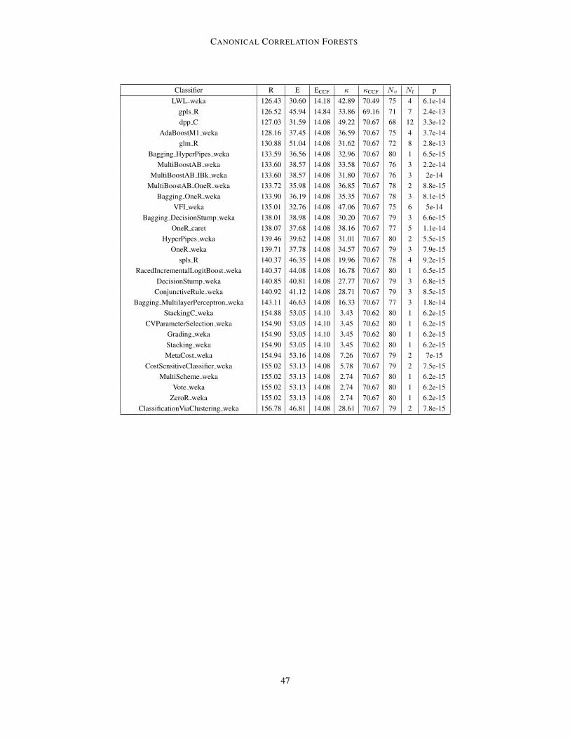
CANONICAL CORRELATION FORESTS

Classifier R E ECCF κ κCCF Nv Nl pLWL weka 126.43 30.60 14.18 42.89 70.49 75 4 6.1e-14

gpls R 126.52 45.94 14.84 33.86 69.16 71 7 2.4e-13dpp C 127.03 31.59 14.08 49.22 70.67 68 12 3.3e-12

AdaBoostM1 weka 128.16 37.45 14.08 36.59 70.67 75 4 3.7e-14glm R 130.88 51.04 14.08 31.62 70.67 72 8 2.8e-13

Bagging HyperPipes weka 133.59 36.56 14.08 32.96 70.67 80 1 6.5e-15MultiBoostAB weka 133.60 38.57 14.08 33.58 70.67 76 3 2.2e-14

MultiBoostAB IBk weka 133.60 38.57 14.08 31.80 70.67 76 3 2e-14MultiBoostAB OneR weka 133.72 35.98 14.08 36.85 70.67 78 2 8.8e-15

Bagging OneR weka 133.90 36.19 14.08 35.35 70.67 78 3 8.1e-15VFI weka 135.01 32.76 14.08 47.06 70.67 75 6 5e-14

Bagging DecisionStump weka 138.01 38.98 14.08 30.20 70.67 79 3 6.6e-15OneR caret 138.07 37.68 14.08 38.16 70.67 77 5 1.1e-14

HyperPipes weka 139.46 39.62 14.08 31.01 70.67 80 2 5.5e-15OneR weka 139.71 37.78 14.08 34.57 70.67 79 3 7.9e-15

spls R 140.37 46.35 14.08 19.96 70.67 78 4 9.2e-15RacedIncrementalLogitBoost weka 140.37 44.08 14.08 16.78 70.67 80 1 6.5e-15

DecisionStump weka 140.85 40.81 14.08 27.77 70.67 79 3 6.8e-15ConjunctiveRule weka 140.92 41.12 14.08 28.71 70.67 79 3 8.5e-15

Bagging MultilayerPerceptron weka 143.11 46.63 14.08 16.33 70.67 77 3 1.8e-14StackingC weka 154.88 53.05 14.10 3.43 70.62 80 1 6.2e-15

CVParameterSelection weka 154.90 53.05 14.10 3.45 70.62 80 1 6.2e-15Grading weka 154.90 53.05 14.10 3.45 70.62 80 1 6.2e-15Stacking weka 154.90 53.05 14.10 3.45 70.62 80 1 6.2e-15MetaCost weka 154.94 53.16 14.08 7.26 70.67 79 2 7e-15

CostSensitiveClassifier weka 155.02 53.13 14.08 5.78 70.67 79 2 7.5e-15MultiScheme weka 155.02 53.13 14.08 2.74 70.67 80 1 6.2e-15

Vote weka 155.02 53.13 14.08 2.74 70.67 80 1 6.2e-15ZeroR weka 155.02 53.13 14.08 2.74 70.67 80 1 6.2e-15

ClassificationViaClustering weka 156.78 46.81 14.08 28.61 70.67 79 2 7.8e-15

47

RAINFORTH AND WOOD

References

Simon Bernard, Laurent Heutte, and Sebastien Adam. Influence of hyperparameters on randomforest accuracy. In MCS, pages 171–180. Springer, 2009.

GASrard Biau. Analysis of a random forests model. Journal of Machine Learning Research, 13(Apr):1063–1095, 2012.

Ake Bjorck and Gene H Golub. Numerical methods for computing angles between linear subspaces.Mathematics of computation, 27(123):579–594, 1973.

Rico Blaser and Piotr Fryzlewicz. Random rotation ensembles. Journal of Machine LearningResearch, 17(4):1–26, 2016.

Magnus Borga. Canonical correlation: a tutorial. On line tutorialhttp://people.imt.liu.se/magnus/cca, 4, 2001.

Leo Breiman. Bagging predictors. Machine learning, 24(2):123–140, 1996.

Leo Breiman. Random forests. Machine learning, 45(1):5–32, 2001.

Leo Breiman, Jerome Friedman, Charles J Stone, and Richard A Olshen. Classification and regres-sion trees. CRC press, 1984.

Gavin Brown, Jeremy Wyatt, Rachel Harris, and Xin Yao. Diversity creation methods: a survey andcategorisation. Information Fusion, 6(1):5–20, 2005.

Jean Carletta. Assessing agreement on classification tasks: the kappa statistic. Computationallinguistics, 22(2):249–254, 1996.

Claude Cohen and Adi Ben-Israel. On the computation of canonical correlations. Cahiers CentreeEtudes Recherche Opeer, 11:121–132, 1969.

Antonio Criminisi, Jamie Shotton, and Ender Konukoglu. Decision forests: A unified frameworkfor classification, regression, density estimation, manifold learning and semi-supervised learning.Foundations and Trends R© in Computer Graphics and Vision, (7):81–227, 2011.

Fernando De la Torre. A least-squares framework for component analysis. Pattern Analysis andMachine Intelligence, IEEE Transactions on, 34(6):1041–1055, 2012.

Glenn De’Ath. Multivariate regression trees: a new technique for modeling species–environmentrelationships. Ecology, 83(4):1105–1117, 2002.

Persi Diaconis and Mehrdad Shahshahani. The subgroup algorithm for generating uniform randomvariables. Probability in the engineering and informational sciences, 1(01):15–32, 1987.

Haytham Elghazel, Alex Aussem, and Florence Perraud. Trading-off diversity and accuracy for op-timal ensemble tree selection in random forests. In Ensembles in Machine Learning Applications,pages 169–179. Springer, 2011.

48

CANONICAL CORRELATION FORESTS

Jean Baptiste Faddoul, Boris Chidlovskii, Remi Gilleron, and Fabien Torre. Learning multiple taskswith boosted decision trees. In Joint European Conference on Machine Learning and KnowledgeDiscovery in Databases, pages 681–696. Springer, 2012.

Manuel Fernandez-Delgado, Eva Cernadas, Senen Barro, and Dinani Amorim. Do we need hun-dreds of classifiers to solve real world classification problems? The Journal of Machine LearningResearch, 15(1):3133–3181, 2014.

Ronald A Fisher. The use of multiple measurements in taxonomic problems. Annals of eugenics, 7(2):179–188, 1936.

Jerome H Friedman. Greedy function approximation: a gradient boosting machine. Annals ofstatistics, pages 1189–1232, 2001.

Joao Gama. Functional trees. Machine Learning, 55(3):219–250, 2004.

Pierre Geurts, Damien Ernst, and Louis Wehenkel. Extremely randomized trees. Machine learning,63(1):3–42, 2006a.

Pierre Geurts, Louis Wehenkel, and Florence d’Alche Buc. Kernelizing the output of tree-basedmethods. In Proceedings of the 23rd international conference on Machine learning, pages 345–352. Acm, 2006b.

Ben Glocker, Olivier Pauly, Ender Konukoglu, and Antonio Criminisi. Joint classification-regression forests for spatially structured multi-object segmentation. Computer Vision–ECCV2012, pages 870–881, 2012.

Gene H Golub and Christian Reinsch. Singular value decomposition and least squares solutions.Numerische mathematik, 14(5):403–420, 1970.

Gene H Golub and Charles F Van Loan. Matrix computations, volume 3. JHU Press, 2012.

Mark Hall, Eibe Frank, Geoffrey Holmes, Bernhard Pfahringer, Peter Reutemann, and Ian H Witten.The weka data mining software: an update. ACM SIGKDD explorations newsletter, 11(1):10–18,2009.

Trevor Hastie, Andreas Buja, and Robert Tibshirani. Penalized discriminant analysis. The Annalsof Statistics, pages 73–102, 1995.

Tin Kam Ho. Random decision forests. In Document Analysis and Recognition, 1995., Proceedingsof the Third International Conference on, volume 1, pages 278–282. IEEE, 1995.

Tin Kam Ho. The random subspace method for constructing decision forests. 20:832–844, 1998.

Harold Hotelling. Relations between two sets of variates. Biometrika, pages 321–377, 1936.

Alston S Householder. Unitary triangularization of a nonsymmetric matrix. Journal of the ACM(JACM), 5(4):339–342, 1958.

Ludmila I Kuncheva and Christopher J Whitaker. Measures of diversity in classifier ensembles andtheir relationship with the ensemble accuracy. Machine learning, 51(2):181–207, 2003.

49

RAINFORTH AND WOOD

Tracy D Lemmond, Andrew O Hatch, Barry Y Chen, David Knapp, Lawrence Hiller, MarshallMugge, and William G Hanley. Discriminant random forests. In DMIN, pages 55–61, 2008.

Jinyan Li and Huiqing Liu. Kent ridge bio-medical data set repository. Institute for InfocommResearch. http://sdmc.lit.org.sg/GEDatasets/Datasets, 2002.

M. Lichman. UCI machine learning repository, 2013.

Henrik Linusson. Multi-output random forests. 2013.

Wei-Yin Loh. Regression tress with unbiased variable selection and interaction detection. StatisticaSinica, pages 361–386, 2002.

Wei-Yin Loh and Yu-Shan Shih. Split selection methods for classification trees. Statistica sinica, 7(4):815–840, 1997.

Gilles Louppe. Understanding random forests: From theory to practice. arXiv preprintarXiv:1407.7502, 2014.

Dragos D Margineantu and Thomas G Dietterich. Pruning adaptive boosting. In ICML, volume 97,pages 211–218, 1997.

Bjoern H Menze, B Michael Kelm, Daniel N Splitthoff, Ullrich Koethe, and Fred A Hamprecht.On oblique random forests. In Machine Learning and Knowledge Discovery in Databases, pages453–469. Springer, 2011.

Marcin Molga and Czesław Smutnicki. Test functions for optimization needs. Test functions foroptimization needs, 2005.

Sreerama K. Murthy, Simon Kasif, and Steven Salzberg. A system for induction of oblique decisiontrees. arXiv preprint cs/9408103, 1994.

Carlos Pardo, Jose F Diez-Pastor, Cesar Garcıa-Osorio, and Juan J Rodrıguez. Rotation forests forregression. Applied Mathematics and Computation, 219(19):9914–9924, 2013.

J. Ross Quinlan. Induction of decision trees. Machine learning, 1(1):81–106, 1986.

J Ross Quinlan. C4. 5: programs for machine learning. Elsevier, 2014.

C Radhakrishna Rao. The utilization of multiple measurements in problems of biological clas-sification. Journal of the Royal Statistical Society. Series B (Methodological), 10(2):159–203,1948.

Marko Robnik-Sikonja. Improving random forests. In Machine Learning: ECML 2004, pages359–370. Springer, 2004.

Juan Jose Rodriguez, Ludmila I Kuncheva, and Carlos J Alonso. Rotation forest: A new classifierensemble method. Pattern Analysis and Machine Intelligence, IEEE Transactions on, 28(10):1619–1630, 2006.

Lior Rokach. Ensemble-based classifiers. Artificial Intelligence Review, 33(1):1–39, 2010.

50

CANONICAL CORRELATION FORESTS

Ferdinando S Samaria and Andy C Harter. Parameterisation of a stochastic model for human faceidentification. In Applications of Computer Vision, 1994., Proceedings of the Second IEEE Work-shop on, pages 138–142, 1994.

Mark Segal and Yuanyuan Xiao. Multivariate random forests. Wiley Interdisciplinary Reviews:Data Mining and Knowledge Discovery, 1(1):80–87, 2011.

Peter Sollich and Anders Krogh. Learning with ensembles: How overfitting can be useful. Advancesin neural information processing systems, pages 190–196, 1996.

Liang Sun, Shuiwang Ji, and Jieping Ye. A least squares formulation for canonical correlationanalysis. In Proceedings of the 25th international conference on Machine learning, pages 1024–1031. ACM, 2008.

Tyler M Tomita, Mauro Maggioni, and Joshua T Vogelstein. Randomer forests. arXiv preprintarXiv:1506.03410, 2015.

Tyler M Tomita, Mauro Maggioni, and Joshua T Vogelstein. Roflmao: Robust oblique forests withlinear matrix operations. In Proceedings of the 2017 SIAM International Conference on DataMining, pages 498–506. Society for Industrial and Applied Mathematics, 2017.

Grigorios Tsoumakas, Ioannis Katakis, and Ioannis Vlahavas. Mining multi-label data. Data miningand knowledge discovery handbook, pages 667–685, 2010.

Michael Wainberg, Babak Alipanahi, and Brendan J Frey. Are random forests truly the best classi-fiers? The Journal of Machine Learning Research, 17(1):3837–3841, 2016.

G Yule. On the association of attributes in statistics, volume a 194. Phil. Trans, pages 257–319,1900.

Heping Zhang. Classification trees for multiple binary responses. Journal of the American Statisti-cal Association, 93(441):180–193, 1998.

Le Zhang and Ponnuthurai Nagaratnam Suganthan. Random forests with ensemble of featurespaces. Pattern Recognition, 47(10):3429–3437, 2014.

51