Lehigh UniversityLehigh Preserve

Theses and Dissertations

2015

Capabilities and Limitations of Infinite-TimeComputationJames Thomas Long IIILehigh University

Follow this and additional works at: http://preserve.lehigh.edu/etd

Part of the Mathematics Commons

This Dissertation is brought to you for free and open access by Lehigh Preserve. It has been accepted for inclusion in Theses and Dissertations by anauthorized administrator of Lehigh Preserve. For more information, please contact preserve@lehigh.edu.

Recommended CitationLong III, James Thomas, "Capabilities and Limitations of Infinite-Time Computation" (2015). Theses and Dissertations. 2694.http://preserve.lehigh.edu/etd/2694

Capabilities and Limitations of Infinite-Time

Computation

by

James Thomas Long III

A Dissertation

Presented to the Graduate Committee

of Lehigh University

in Candidacy for the Degree of

Doctor of Philosophy

in

Mathematics

Lehigh University

May 2015

Copyright c© 2015 by James Thomas Long III

ii

Approved and recommended for acceptance as a dissertation in partial fulfillment

of the requirements for the degree of Doctor of Philosophy.

James Thomas Long III

Capabilities and Limitations of Infinite-Time Computation

Date

Lee Stanley, Ph.D.

Dissertation Director

Committee Chair

Accepted Date

Committee Members:

Vincent Coll, Ph.D.

Michael Fraboni, Ph.D.

Garth Isaak, Ph.D.

Terrence Napier, Ph.D.

iii

Acknowledgments

Throughout the research, writing, and defense of this dissertation, I have been

blessed to have the support of numerous people. While I will not soon forget their

integral contributions, they deserve to be recognized here for all to see.

My advisor, Professor Lee Stanley, has been a pleasure to talk to and work

with ever since I met him, purely by chance, the day after I found out that I was

accepted to Lehigh’s graduate program. I am confident that this dissertation is

but the first of many academic adventures for us.

Not only did my committee members all selflessly provide helpful comments

and feedback throughout the process, but they all brought their own special

contributions to the table:

• Professor Vince Coll was always a source of fruitful intellectual conversations

and sage advice. I look forward to continuing our collaboration on any

number of projects in the future.

• After Professor Garth Isaak asked a seemingly innocuous question during my

general exam (“What happens when classical Turing machines are allowed

to modify their own instruction lists?”), I was inspired to formulate variants

of self-modifying infinite-time Turing machines and undertake a thorough

investigation into their behavior, which is all summarized in Chapter 5. I

encourage him to keep the questions up!

• Professor Terry Napier has been a wonderful mentor throughout my entire

time at Lehigh. In addition, he introduced me to the curious, but highly

appropriate, word “scholium,” which is used throughout Chapter 2.

iv

• Professor Mike Fraboni of Moravian College was the first person to seriously

suggest that I consider graduate school in mathematics, and gave me my

first exposure to mathematical research. I am grateful to have him back for

one last hurrah.

I was extremely fortunate to learn the fundamentals of infinitary computability

from one of the founding fathers of the field, Joel David Hamkins. Not only did

Joel patiently address any and all questions I had about the basic theory, but he

also suggested that I consider infinite-time formulations of Rado’s busy beaver

problem; indeed, this advice led to much of the content of Chapter 3.

Special thanks are due to the entire Lehigh community. Many would claim that

the math department faculty and staff are uniformly supportive of the graduate

student cause, and my experiences have been no exception. I am especially

appreciative of all that Mary Ann Dent, our beloved department coordinator, did

for me when I was getting acclimatized to graduate life. Finally, Kathleen Hutnik’s

unparalleled care for all the graduate students of Lehigh, and especially for me,

cannot be overstated.

The friendships I have made with my fellow graduate students have been one

of the most meaningful aspects of my graduate career. Of all the people I could list

here, I will settle on singling out three: the first two provided valued camaraderie

and technical contributions to the writing process and defense, and the last is used

to me embarrassing her with public acknowledgments!

• My “brother” Bill Franczak was a constant source of humor and fruitful

discussions about any number of topics, be it logic, computer science, or

Five Nights at Freddy’s. I also greatly appreciate him “Skyping in” my old

friend Patty Garmirian for my defense.

• In addition to being a stellar friend to both me and Lindsey, Bob Short

introduced me to the online Overleaf LATEX editor when I was starting to

write up my manuscript. Overleaf was exactly what I needed to prepare my

dissertation in a timely fashion!

v

• Throughout six unforgettable years of friendship, Rivka Win has provided

me more moral support and laughter (not to mention hand sanitizer) than

all of the other graduates combined. Now more than ever, I am thankful for

asking her if she wanted to study for the comprehensive exams together!

I will miss her, but look forward to keeping in touch with her as much as

possible.

My family (biological, step, and future in-law alike) not only emotionally

supported me throughout the trials and tribulations of graduate school, but also

set an example for me to follow long before I set foot on campus. I look forward

to being able to call home more often!

Not surprisingly, but no less appreciated, my sister Becky was especially

supportive. Every Sunday, I could always count on her being a sounding board

for all of my most important considerations, and always enjoyed the chance to

do the same for her. While many of our conversations as of late have involved

lamenting the stresses that growing up brings, I would like to think that we’ve

grown up quite nicely.

Last, but certainly not least, I am indebted to my beloved fiancee Lindsey,

whose constant presence in my life gave meaning and purpose to this undertaking

of mine. I could always count on her to inspire me to think outside the box when

I was invariably faced with a seemingly insurmountable obstacle. Put simply:

thank you to her for being the circumference to my radius, and the Law of Cosines

to my Pythagorean Theorem. Our marriage, and indeed, the rest of our lives,

could not come soon enough.

vi

Contents

List of Figures ix

Abstract 1

1 Introduction 3

1.1 Notation And Preliminaries . . . . . . . . . . . . . . . . . . . . . . . 3

1.1.1 Product Spaces . . . . . . . . . . . . . . . . . . . . . . . . . . 3

1.1.2 Coding Relations on N . . . . . . . . . . . . . . . . . . . . . . 4

1.1.3 Operations on Partial Functions . . . . . . . . . . . . . . . . 4

1.1.4 Infinite-Time Turing Machines . . . . . . . . . . . . . . . . . 6

1.1.5 Writable, Eventually Writable, and Accidentally Writable

Reals . . . . . . . . . . . . . . . . . . . . . . . . . . . . . . . . 10

1.1.6 Relativized Infinite-Time Computation . . . . . . . . . . . . 10

1.2 Context and Motivation . . . . . . . . . . . . . . . . . . . . . . . . . 11

1.2.1 Rado’s Busy Beaver Functions . . . . . . . . . . . . . . . . . 12

1.2.2 Fast-Growing Hierarchies of Finite-Time

Computable Functions . . . . . . . . . . . . . . . . . . . . . . 12

1.2.3 Self-Modifying Models of Finitary Computation . . . . . . . 13

1.3 Results and Organization . . . . . . . . . . . . . . . . . . . . . . . . 14

2 Some Useful Infinite-Time Turing Machine Tools and Constructs 15

2.1 Extending the Classical Finite-Time Operations

of Computability to the Infinite-Time Setting . . . . . . . . . . . . . 16

vii

2.2 Employing Extra Tapes . . . . . . . . . . . . . . . . . . . . . . . . . . 19

2.3 Implementing Flags . . . . . . . . . . . . . . . . . . . . . . . . . . . . 25

3 A Busy Beaver Problem for Infinite-Time Turing Machines 32

3.1 Extending Σ to Infinite-Time Turing Machines . . . . . . . . . . . . 33

3.2 Some Domination Results for Σ∞ and Σe∞ . . . . . . . . . . . . . . . 34

3.3 The Infinite-Time Degree of Σ∞ and Σe∞ . . . . . . . . . . . . . . . . 40

4 A Fast-Growing Hierarchy Based on Infinite-Time Turing Machines 44

4.1 Review of Fast-Growing Hierarchies and Ordinal Notation . . . . . 44

4.2 Systems of Ordinal Notations up toωCK1 , λ, and ζ . . . . . . . . . . 47

4.3 The Fast-Growing Hierarchy Induced by the Q++-Notations . . . . 51

5 Two Variants of Self-Modifying Infinite-Time Turing Machines 57

5.1 Self-Modification of Instructions . . . . . . . . . . . . . . . . . . . . 58

5.2 Passing from Class I to Class ILT SMITTMs . . . . . . . . . . . . . . 63

5.3 Developing the Theory for Class ILT SMITTMs . . . . . . . . . . . . 73

6 Conclusions and Future Work 78

6.1 Conclusions and Future Work Based on Chapter 3 . . . . . . . . . . 78

6.2 Conclusions and Future Work Based on Chapter 4 . . . . . . . . . . 79

6.3 Conclusions and Future Work Based on Chapter 5 . . . . . . . . . . 80

6.4 Another Avenue for Future Work . . . . . . . . . . . . . . . . . . . . 81

Index 82

Bibliography 85

Vita 88

viii

List of Figures

1.1 A 3-tape ITTM . . . . . . . . . . . . . . . . . . . . . . . . . . . . . . . 7

2.1 3-tape ITTM simulation of a 4-tape ITTM . . . . . . . . . . . . . . . 24

2.2 8-tape ITTM simulation of a 4-tape ITTM with 2 FLAGS . . . . . . . 30

5.1 Class I SMITTM with 3 data tapes . . . . . . . . . . . . . . . . . . . 60

5.2 Class ILT SMITTM . . . . . . . . . . . . . . . . . . . . . . . . . . . . 68

ix

Abstract

The relatively new field of infinitary computability strives to characterize the

capabilities and limitations of infinite-time computation; that is, computations of

potentially transfinite length. Throughout our work, we focus on the prototypical

model of infinitary computation: Hamkins and Lewis’ infinite-time Turing ma-

chine (ITTM), which generalizes the classical Turing machine model in a natural

way.

This dissertation adopts a novel approach to this study: whereas most of the

literature, starting with Hamkins and Lewis’ debut of the ITTM model, pursues

set-theoretic questions using a set-theoretic approach, we employ arguments that

are truly computational in character. Indeed, we fully utilize analogues of classical

results from finitary computability, such as the smn Theorem and existence of

universal machines, and for the most part, judiciously restrict our attention to the

classical setting of computations over the natural numbers.

In Chapter 2 of this dissertation, we state, and derive, as necessary, the afore-

mentioned analogues of the classical results, as well as some useful constructs

for ITTM programming. With this due paid, the subsequent work in Chapters 3

and 4 requires little in the way of programming, and that programming which is

required in Chapter 5 is dramatically streamlined. In Chapter 3, we formulate two

analogues of one of Rado’s busy beaver functions from classical computability,

and show, in analogy with Rado’s results, that they grow faster than a wide class of

infinite-time computable functions. Chapter 4 is tasked with developing a system

of ordinal notations via a natural approach involving infinite-time computation,

1

as well as an associated fast-growing hierarchy of functions over the natural num-

bers. We then demonstrate that the busy beaver functions from Chapter 3 grow

faster than the functions which appear in a significant portion of this hierarchy.

Finally, we debut, in Chapter 5, two enhancements of the ITTM model which

can self-modify certain aspects of their underlying software and hardware mid-

computation, and show the somewhat surprising fact that, under some reasonable

assumptions, these new models of infinitary computation compute precisely the

same functions as the original ITTM model.

2

Chapter 1

Introduction

1.1 Notation And Preliminaries

1.1.1 Product Spaces

Definition 1.1.1. 2N shall denote Cantor space (i.e., the set of countably long

binary sequences with index N).

The elements of Cantor space will often be called real numbers, or simply

reals. ♦

Definition 1.1.2. A product space X is a finite Cartesian product of the form

X = X1 × X2 × · · · × Xk, where each Xi is either N or 2N.

In the event that each Xi = N, we say that X is a type 0 product space. Other-

wise, X is said to be a type 1 product space.

A pointclass Λ is a collection of sets such that each P ∈ Λ is a subset of some

product space X (potentially depending on P). ♦

Remark. We typically denote an arbitrary product space by calligraphic letters,

such as X, Y, or Z. 4

Definition 1.1.3. We define the products of product spaces by setting

X× Y = X1 × · · · × Xk × Y1 × · · · × Yl

3

whenever X = X1 × · · · × Xk and Y = Y1 × · · · × Yl.We similarly define the pairing of product space points by setting

(x, y) = (x1, . . . , xk, y1, . . . , yl)

whenever x = (x1, . . . , xk) and y = (y1, . . . , yl). ♦

1.1.2 Coding Relations on N

For the remainder of this dissertation, we fix a Godel coding for N× N.

Definition 1.1.4. For every x ∈ 2N, let ≺x denote the relation coded by x =

(x0, x1, x2, . . .). That is,m ≺x n if and only if xi = 1, where i is the Godel code for

(m,n). ♦

Definition 1.1.5. For every x ∈ 2N and n ∈ N, let rest (x, n) denote the real

coding of ≺x �n (i.e., the real which codes the restriction of ≺x to the set of all

≺x-predecessors of n). ♦

1.1.3 Operations on Partial Functions

As is typical for all branches of computability, partial functions will serve as one

of our primary objects of study.

Definition 1.1.6. A partial function f : X→ Y is a function with domain a subset

of X and codomain Y.

In the event that dom (f) = X, we call f a total function. ♦

When comparing partial functions, it is important to consider not just where

they agree, but also where they are mutually undefined.

Definition 1.1.7. Let f : X → Y and g : X → Y be partial functions. Then we

write f(x) ' g(x) if for every x ∈ X, either (1) f(x) and g(x) are both defined and

f(x) = g(x) or (2) f(x) and g(x) are both undefined. ♦

4

Definition 1.1.8. Let f : N → N and g : N → N be total functions. We say that

f eventually dominates g, or that f(n) >∗ g(n), if f(n) > g(n) for n sufficiently

large. ♦

We now state the three partial recursive operations from finite-time computabil-

ity. We will see in Chapter 2 that they will be among our most useful high-level

tools.

Definition 1.1.9. Let n ∈ N, and let g : Yn → Z and h1 : X → Y, h2 : X → Y, . . .,

hn : X→ Y be partial functions.

Then the partial function f : X→ Z given by f(x) ' g (h1(x), h2(x), . . . , hn(x))is said to be obtained by substitution from g, h1, h2, . . ., hn. ♦

Definition 1.1.10. Let g : X→ X and h : N× X× X→ X be partial functions.

Then the partial function f : N× X→ X defined by

f(0, x) ' g(x)

f(n+ 1, x) ' h (n, f(n, x), x)

is said to be obtained by primitive recursion from g and h. ♦

Definition 1.1.11. Let g : N× X→ Y be a partial function.

Then the partial function f : X→ N given by

f(x) := µn (g(n, x) = 0)

=

n if g(n, x) = 0 and g(m,x) is defined and

nonzero for allm < n

undefined if there is no such n

is said to be obtained by unbounded minimization from g. ♦

Remark. Some authors refer to the µ operator as being an “unbounded search

operator,” and for good reason. Indeed, [Rog67] uses the following Church-

Turing Thesis argument to show that f is finite-time computable provided that g

is: systematically compute g(0, x), g(1, x), g(2, x), . . . until and unless a witness

n ∈ N is found such that g(n, x) = 0. 4

5

Definition 1.1.12. The class of primitive recursive functions arises by closing the 0

function, successor function, and projection functions Uni (k1, . . . , ki, . . . , kn) := kiunder substitution and primitive recursion. ♦

1.1.4 Infinite-Time Turing Machines

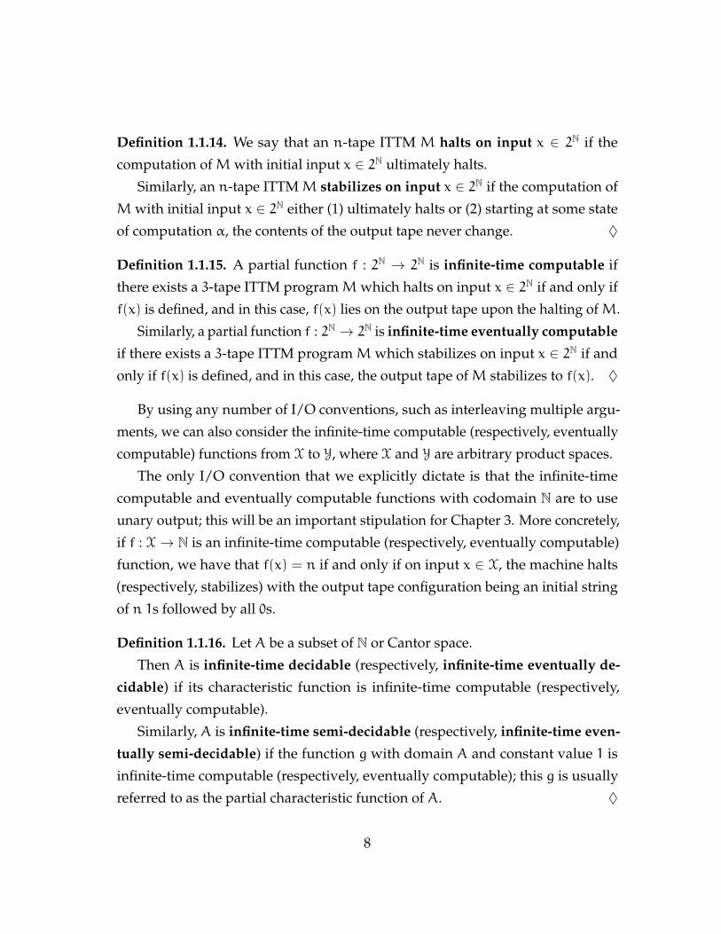
Definition 1.1.13. A standard infinite-time Turing machine with n tapes (or n-

tape ITTM)M possesses the following hardware (see Figure 1.1 on page 7 for an

illustration):

1. n (one-sidedly infinite) tapes with cells indexed by N, each of which can

store the values “0” or “1.” Two of these tapes (potentially equal to each

other) are predesignated for input and output.

2. A one-cell-wide head for reading and writing, which is superimposed over

the same cell of each tape simultaneously.

3. A finite number of states S1, S2, . . ., Sk, as well as the two special states

HALT and LIMIT .

If an ITTM is not explicitly specified as “n-tape,” it is to be assumed that

n = 3. The typical names given to the tapes in this case are INPUT ,OUTPUT , and

SCRATCH.

Before execution, M is loaded with a program consisting of finitely many

instructions, each of which has a prefix and suffix.

• The prefixes are of the form S a0a1 · · ·an−1, where S is a state ofM. (Taken

to read “If we are in state S and we are reading the bits a0, a1, . . . , an−1 on

the tapes...”)

• The suffixes are of the form a0a1 · · ·an−1 L S or a0a1 · · ·an−1 R S, where S

is a non-limit state of M. (Taken to read “... write the bits a0, a1, . . . , an−1to the tapes, move the head to the left [respectively, right], and transition to

state S.”)

6

(It is assumed thatM’s program has exactly one instruction for each possible

prefix.)

Upon execution,M acts as a finite-time Turing machine does during successor

steps of computation:

1. M consults its program to find the unique instruction with the relevant

prefix.

2. M then does as the corresponding suffix dictates. More specifically,

(a) Mwrites the bits indicated by the suffix.

(b) Mmoves its tape head in the specified direction.

(c) M either transitions to the state S from the suffix (if S 6= HALT ) or halts

(if S = HALT ).

During limit steps of computation,M does the following:

1. All cells assume the lim sup of their preceding values.

2. The tape head moves to the left-hand side of the tapes.

3. The state is changed to the LIMIT state.

♦

Remark. The contents of any tape at any stage of computation are naturally viewed

as an element of Cantor space. 4

INPUT 1 0 0 1 1 0 1 · · ·OUTPUT 1 1 1 0 1 0 0 · · ·

SCRATCH 1 0 1 0 0 0 1 · · ·

Figure 1.1: A 3-tape ITTM. Here, the tape head is superimposed over cell array 1.

There are two natural ways to define infinite-time computable functions, both

of which stem from two different types of output convention.

7

Definition 1.1.14. We say that an n-tape ITTM M halts on input x ∈ 2N if the

computation ofMwith initial input x ∈ 2N ultimately halts.

Similarly, an n-tape ITTMM stabilizes on input x ∈ 2N if the computation of

Mwith initial input x ∈ 2N either (1) ultimately halts or (2) starting at some state

of computation α, the contents of the output tape never change. ♦

Definition 1.1.15. A partial function f : 2N → 2N is infinite-time computable if

there exists a 3-tape ITTM programMwhich halts on input x ∈ 2N if and only if

f(x) is defined, and in this case, f(x) lies on the output tape upon the halting of M.

Similarly, a partial function f : 2N → 2N is infinite-time eventually computable

if there exists a 3-tape ITTM program M which stabilizes on input x ∈ 2N if and

only if f(x) is defined, and in this case, the output tape ofM stabilizes to f(x). ♦

By using any number of I/O conventions, such as interleaving multiple argu-

ments, we can also consider the infinite-time computable (respectively, eventually

computable) functions from X to Y, where X and Y are arbitrary product spaces.

The only I/O convention that we explicitly dictate is that the infinite-time

computable and eventually computable functions with codomain N are to use

unary output; this will be an important stipulation for Chapter 3. More concretely,

if f : X→ N is an infinite-time computable (respectively, eventually computable)

function, we have that f(x) = n if and only if on input x ∈ X, the machine halts

(respectively, stabilizes) with the output tape configuration being an initial string

of n 1s followed by all 0s.

Definition 1.1.16. Let A be a subset of N or Cantor space.

Then A is infinite-time decidable (respectively, infinite-time eventually de-

cidable) if its characteristic function is infinite-time computable (respectively,

eventually computable).

Similarly, A is infinite-time semi-decidable (respectively, infinite-time even-

tually semi-decidable) if the function g with domain A and constant value 1 is

infinite-time computable (respectively, eventually computable); this g is usually

referred to as the partial characteristic function of A. ♦

8

Remark. In the sequel and in the literature, partially decidable and semi-decidable

are used interchangeably. 4

For the remainder of this dissertation, we fix a Godel numbering of 3-tape

ITTM programs.

Definition 1.1.17. Let ϕp (respectively, ϕep) denote the partial function from 2N

to 2N which is infinite-time computed (respectively, eventually computed) by the

3-tape ITTM with program code p. ♦

Definition 1.1.18. Let ϕ(X,Y)p (respectively, ϕe,(X,Y)p ) denote the partial function

from X to Y which is infinite-time computed (respectively, eventually computed)

by the 3-tape ITTM with program code p. ♦

In Chapter 4, we will employ both finite-time and infinite-time computable

functions, so let us also introduce special notation for the finite-time computable

functions:

Definition 1.1.19. Let ft-ϕp denote the pth finite-time computable function. ♦

We can now state analogues of some of the central theorems of finite-time

computability; they will be extremely helpful for our purposes in particular.

Theorem 1.1.20 (smn Theorem for ITTMs; Hamkins and Lewis [HL00]). Let X be a

type 0 product space.

Then there exists a primitive recursive s : N × X → N such that for every #»n ∈ X,

y ∈ Y, and p ∈ N,

ϕ(X×Y,Z)p ( #»n, y) ' ϕ(Y,Z)

s(p, #»n)(y) and ϕe,(X×Y,Z)p ( #»n, y) ' ϕe,(Y,Z)

s(p, #»n) (y).

Theorem 1.1.21 (Universal Machines for ITTMs; Hamkins and Lewis [HL00]). Let

X,Y be product spaces. Then the mapsϕU,(X,Y) : N×X→ Y andϕU,e,(X,Y) : N×X→ Y

which are respectively given by

ϕU,(X,Y)(n, x) ' ϕ(X,Y)n (x) and ϕU,e,(X,Y)(n, x) ' ϕe,(X,Y)n (x)

are infinite-time computable and eventually computable, respectively.

9

Theorem 1.1.22 (Second Recursion Theorem for ITTMs; Hamkins and Lewis

[HL00]). Let f : N → N be total infinite-time computable (respectively, eventually

computable). Then there exists an index p ∈ N such that for every pair of product spaces

X, Y, we have that ϕ(X,Y)f(p) = ϕ

(X,Y)p (respectively, ϕe,(X,Y)f(p) = ϕ

e,(X,Y)p ).

1.1.5 Writable, Eventually Writable, and Accidentally Writable

Reals

Definition 1.1.23. Let ωCK1 be the Church-Kleene ordinal; i.e., the supremum

of the recursive ordinals (those countable ordinals which are lengths of some

well-ordering of N whose graph is finite-time decidable). ♦

Definition 1.1.24. An ITTM tape is considered blank if it is completely filled with

0s. ♦

Definition 1.1.25. A real x ∈ 2N is writable (respectively, eventually writable)

if there exists an ITTM, which, starting from blank input, ultimately halts on

(respectively, stabilizes to) output x.

Similarly, a real x ∈ 2N is accidentally writable if there exists an ITTM, which,

starting from blank input, has x on its output tape at some point in the computa-

tion.

An ordinal α is said to be writable, eventually writable, or accidentally

writable if it has a real code x which is writable, eventually writable, or acci-

dentally writable, respectively. ♦

Definition 1.1.26. Let λ, ζ, and Σ denote the supremum of the writable, eventually

writable, and accidentally writable ordinals, respectively. ♦

1.1.6 Relativized Infinite-Time Computation

Infinite-time Turing machines admit two natural notions of oracles: single real

numbers z ∈ 2N (or equivalently, subsets of N) and subsets of real A ⊆ 2N.

10

The former are handled in the same fashion as in the finite-time setting: one

appends a (read-only) ORACLE tape preloaded with z to the ITTM, and during

successor steps, the ITTM also reads a bit from the ORACLE to assess which

instruction to execute.

As for the latter, we append a blank ORACLE tape to the ITTM. During every

successor step, the oracle indicates if the current real on the ORACLE tape is an

element of A, and the tape head also reads a bit from the ORACLE tape; the ITTM

then acts accordingly. Moreover, in the course of executing a successor step, the

ITTM will also write a bit to the ORACLE tape.

Definition 1.1.27. Let A and B both be subsets of either N or Cantor space.

1. We say that A is infinite-time reducible to B and write A 6∞ B if the

characteristic function of A is B-computable. If we also know that B 66∞ A,

then we can in fact say that A <∞ B.

2. We further say that A and B have the same infinite-time degree and write

A ≡∞ B if A 6∞ B and B 6∞ A.

♦

Definition 1.1.28. Let z ∈ 2N. Then we denote the weak jump for z by

zO = {p ∈ N the ITTM program with index p and oracle z halts on blank input}.

♦

1.2 Context and Motivation

Starting with the very introduction of the infinite-time Turing machine model in

[HL00], most papers in infinitary computability have strongly emphasized set

theoretic techniques and concerns. In [Wel00a], for instance, Welch showed that

the infinite-time decidable subsets of N (i.e., reals) are precisely the reals at the

level Lλ of the constructible hierarchy. In proving this result, Welch had to employ

11

not just facts about the constructible universe, but also highly technical results

from admissibility theory.

In contrast, our results are directly inspired by natural problems and concepts

from finitary computability, and in the spirit of the classical theory, our proofs are

truly computational in character. Indeed, throughout this entire work, we take

full advantage of the infinite-time Turing machine analogues for the smn Theorem

and universal theorems (as given above), as well as closure of the infinite-time

computable (and eventually computable) functions under the partial recursive

operations, which we shall establish in Chapter 2.

1.2.1 Rado’s Busy Beaver Functions

In his seminal paper [Rad62], Rado exhibited two natural examples of functions

which are not finite-time computable, commonly denoted S and Σ. While these

“busy beaver functions” were seen to be intimately connected to the Halting Prob-

lem, their noncomputability was demonstrated in a more constructive fashion:

whereas the traditional proof of the Halting Problem relies on a proof by contradic-

tion hinging on a diagonal construction, Rado showed directly that his busy beaver

functions grew faster (in the sense of eventual domination) than any finite-time

total computable function.

Chapter 3 will be tasked with generalizing the Σ busy beaver function to

infinite-time computable and eventually computable functions. In particular, we

will see that, not only does Rado ’s eventual domination result extend nicely to our

generalizations, but the infinite-time degree of our generalizations are naturally

tied to the weak jump operator.

1.2.2 Fast-Growing Hierarchies of Finite-Time

Computable Functions

In [Grz53], Grzegorczyk stratified the primitive recursive functions into an increas-

ing family of sets of functions 〈En n < ω〉, and also formulated an associated

12

sequence of functions fn : N → N (n < ω). Sometime later, Lob and Wainer

extended this “Grzegorczyk hierarchy” into a “fast-growing hierarchy” of quickly

increasing functions fα : N→ N (α < ε0, where ε0 is the least ordinal ε such that

ε = ωε; see also [LW70] for further details). In doing so, Grzegorczyk, Lob, and

Wainer cultivated a natural method of classifying the growth rate of finite-time

computable functions.

In light of the busy beaver functions which we defined in Chapter 3, we have a

clear interest in extending the fast-growing hierarchy into the setting of infinite-

time; we do so in Chapter 4, and situate our busy beaver analogues on this new

hierarchy.

1.2.3 Self-Modifying Models of Finitary Computation

The notion of a finitary model of computation which is capable of modifying

its own instruction list has always been “on the horizon” in the computability

literature. Indeed, one of Turing’s prototypical models of computation allowed

for such self-modification (see [Tur36]).

Moreover, self-modification is more than just a mere academic novelty: many

modern programming languages, such as Python, allow for “on the fly” modi-

fication of a program’s instructions. Moreover, the modified Harvard computer

architecture which is standard for modern computers was invented to, among

other things, allow for such self-modification (see [GCC04] for more details).

With this motivation in mind, we formulate, in Chapter 5, two different notions

of self-modification for infinite-time Turing machines and make the satisfying find

that, under some reasonable and necessary assumptions, such self-modification

does not affect the intrinsic computational power of original infinite-time Turing

machine model.

13

1.3 Results and Organization

In Chapter 2, we prove several technical lemmata that greatly simplify our ar-

guments in the sequel. Among other things, we will show that the infinite-time

computable and eventually computable functions are closed under the partial

recursive operations from classical computability theory, and also introduce a

modest new model of infinite-time computation, the ITTM with FLAGS, which is

seen to computationally equivalent to the original model.

Chapter 3 formulates natural analogues Σ∞ and Σe∞ of Rado’s busy beaver

function Σ. Our core result in this chapter shows that Σ∞ and Σe∞ actually enjoy

the same sort of eventual domination property as the Σ function. After providing

some rather striking asymptotic lower bounds for Σ∞ and Σe∞, we then analyze

the infinite-time degrees thereof.

In Chapter 4, we construct a fast-growing hierarchy for all ordinals below ζ.

We then prove that certain tiers of this new hierarchy are effective in a precise

sense, and then use this effectiveness to find large initial segments of the hierarchy

which our busy beaver functions Σ∞ and Σe∞ eventually dominate.

Our last group of results lies in Chapter 5. Here, we devise two different

variants of Self-Modifying Infinite-time Turing Machines, and verify that certain

reasonable subclasses of their computable and eventually computable functions

coincide with that of the infinite-time computable and eventually computable

functions, respectively.

Lastly, Chapter 6 gives a brief summary of what we have accomplished, and

then enumerates the many possible directions for future work. By this point, we

hope the reader will agree that our computational focus opens a number of paths

to further investigation of interesting and natural questions suggested by our

results.

14

Chapter 2

Some Useful Infinite-Time Turing

Machine Tools and Constructs

Before we discuss and prove our main results, it will be very useful to formulate

and prove some versatile technical lemmata which will not only serve to streamline

all of our core arguments, but which are also of interest in their own right, both

intrinsically and with an eye towards future work.

More concretely, we will first see that, just as in the setting of finite-time

computability, the infinite-time computable and eventually computable functions

are closed under the three partial recursive operations which we summarized in

Chapter 1; this is the content of Theorems 2.1.1, 2.1.3, and 2.1.4. Not only will these

results simplify some of the proofs which arise in Chapters 3 and 5, but we will

use them to give completely programming-free proofs of the results of Chapter 4.

Secondly and lastly, we give, in Sections 2.2 and 2.3, two modest (and compu-

tationally equivalent) extensions of the ITTM model which will allow us to more

easily carry out the simulations needed for the results of Chapter 5.

15

2.1 Extending the Classical Finite-Time Operations

of Computability to the Infinite-Time Setting

Given the essential role that function composition and its multivariable analogues

play in all branches of mathematics, it is little surprise that other people have al-

ready handled the closure of infinite-time computable and eventually computable

functions under substitution; see [CH13] and [Kle07] for details.

Theorem 2.1.1 (Coskey and Hamkins, Klev). If a partial function f : X → Z is ob-

tained by substitution from infinite-time computable (respectively, eventually computable)

functions g : Yn → Z and h1 : X → Y, h2 : X → Y, . . ., hn : X → Y, then f is itself

infinite-time computable (respectively, eventually computable).

Theorem 2.1.1 and the following consequence of the Second Recursion Theorem

will be the key to establishing closure under the other two types of partial recursive

operations, as we shall see that both of these operations can be defined via suitable

choice of recursion equation.

Lemma 2.1.2. Let f : N× X→ Y be infinite-time computable (respectively, eventually

computable). Then there exists an index p ∈ N such that for all x ∈ X, ϕ(X,Y)p (x) '

f(p, x) (respectively, ϕe,(X,Y)p (x) ' f(p, x)).

Proof. The proof is identical to that employed in the finite-time setting: the sim-

plified version of the smn Theorem provides a primitive recursive k : N→ N such

that ϕ(X,Y)k(n) (x) ' f(n, x) (respectively, ϕe,(X,Y)k(n) (x) ' f(n, x)). Because k is total

computable, the Second Recursion Theorem for infinite-time computable (respec-

tively, eventually computable) functions then guarantees an index p ∈ N such that

ϕ(X,Y)p = ϕ

(X,Y)k(p) (respectively, ϕe,(X,Y)p = ϕ

e,(X,Y)k(p) ). Fixing such a p gives us the

desired conclusion.

Remark. Loosely speaking, this lemma provides rigorous justification that certain

kinds of self-referential definitions yield perfectly valid infinite-time computable

(and eventually computable) functions. 4

16

With these results established, it is straightforward to demonstrate closure

under primitive recursion.

Theorem 2.1.3. If a partial function f : N× X→ X is obtained by primitive recursion

from infinite-time computable (respectively, eventually computable) functions g : X→ X

and h : N×X×X→ X, then f is itself infinite-time computable (respectively, eventually

computable).

Proof. We will restrict our attention to proving this for infinite-time computable

functions, as the proof in the eventually computable setting carries through mutatis

mutandis.

Let f ′ : N× N× X→ X be defined thusly:

f ′(p, n, x) '

g(x) if n = 0

h(n ′, ϕ

(N×X,X)p (n ′, x), x

)if n = n ′ + 1.

Note that, by closure under substitution and the infinite-time computability of

the relevant universal function, f ′ is infinite-time computable. Now apply Lemma

2.1.2 to obtain an index p ∈ N such that ϕ(N×X,X)p = f ′(p, ·, ·).

It is now clear that f = ϕ(N×X,X)p , and hence f is infinite-time computable, as

desired.

Demonstrating closure under unbounded minimization requires only slightly

more work than was required to prove Theorem 2.1.3.

Theorem 2.1.4. If a partial function f : X→ N is obtained by unbounded minimization

from an infinite-time computable (respectively, eventually computable) partial function

g : N × X → Y, then it is itself infinite-time computable (respectively, eventually

computable).

Proof. As with the preceding proof, there is no loss of generality in only giving the

argument for infinite-time computable functions.

17

Let h ′ : N× N× X→ N be defined as follows:

h ′(p, n, x) '

0 if g(n, x) = 0

ϕ(N×X,N)p (n+ 1, x) + 1 if g(n, x) is defined and nonzero

undefined otherwise.

By closure under substitution and the infinite-time computability of the rele-

vant universal function, h ′ is infinite-time computable. Thus, we may fix an index

p ∈ N as guaranteed by Lemma 2.1.2 so that ϕe,(N×X,Y)p = h ′(p, ·, ·).We now take h = ϕ

e,(N×X,Y)p , which is readily seen to satisfy the following

recursion:

h(n, x) '

0 if g(n, x) = 0

h(n+ 1, x) + 1 if g(n, x) is defined and nonzero

undefined otherwise.

From these equations, one can easily verify that

h(n, x) = m⇔ µz (g(n+ z, x) = 0) = m,

whence f = h(0, ·) is infinite-time computable.

The following corollary justifies our main application of unbounded minimiza-

tion in the sequel.

Corollary 2.1.5. Let P(n, x) be a decidable (respectively, eventually decidable) predicate

over N× X. Then the function f : X→ N given by

f(x) := µn (P(n, x))

=

the least n such that P(n, x) holds if P(n, x) holds for some value of n

undefined otherwise

is eventually computable.

Proof. Let 1P : N × X → N denote the characteristic function of P(n, x), and let

g : N× X→ N be given by g(n, x) = |1P(n, x) − 1|. By closure under substitution,

g is infinite-time computable (respectively, eventually computable). Now simply

observe that µn (P(n, x)) = µn (g(n, x) = 0) and apply Theorem 2.1.4.

18

2.2 Employing Extra Tapes

In [HS01], Hamkins and Seabold demonstrated the curious fact that the ITTMs

with only one tape are, in some sense, not as powerful as their n-tape (for n > 2)

counterparts: while 1-tape and 3-tape ITTMs enjoy the same decidable subsets,

there are functions which are 3-tape-ITTM-computable but not 1-tape-ITTM-

computable. In fact, the 1-tape-ITTM-computable functions are not even closed

under composition!

Luckily, Hamkins and Seabold showed that this peculiar behavior is limited to

the setting of 1-tape ITTMs, as stated precisely below.

Theorem 2.2.1 (Hamkins and Seabold). Let n > 2. Then the n-tape ITTMs and 3-tape

ITTMs compute precisely the same partial functions f : X→ Y.

The upshot of Theorem 2.2.1 is that we can, in the interest of ease of imple-

mentation and/or clarity, design our infinite-time algorithms using more than just

the standard array of 3 tapes. As such, it will be helpful to have an analogue of

Theorem 2.2.1 for infinite-time eventually computable functions.

Theorem 2.2.2. Let n > 3. Then the n-tape ITTMs and 3-tape ITTMs eventually

compute precisely the same partial functions f : X→ Y.

Once we have proven Theorem 2.2.2, we shall see that it is not hard to pass to

a natural relativization thereof:

Theorem 2.2.3. Let n > 3, and z ∈ 2N. Then the n-tape ITTMs and 3-tape ITTMs

z-compute (and eventually z-compute) precisely the same partial functions f : X→ Y.

The same is true with A ⊆ 2N in place of z ∈ 2N.

To prove Theorem 2.2.2, we will first give a (proprietary) proof of 2.2.1 for

n > 3 that extends easily to the setting of infinite-time eventually computable

functions.

Proof of Theorem 2.2.1 for n > 3. Let f : X→ Y be an arbitrary partial function.

19

If f is computable via a 3-tape ITTM, it is clearly computable via an n-tape

ITTM.

Conversely, assume that f is computable via an n-tape ITTMM. Fix such an

M. We will describe a 3-tape ITTMM ′ which, upon being given an input x ∈ X,

halts precisely whenMwould, and in this event returns f(x) as output; in other

words,M ′ infinite-time-computes f.

Without loss of generality, assume the output and input tapes ofM are tapes 0

and 1, respectively.

Now letM ′ be a 3-tape ITTM. For convenience, we shall call the tapes ofM ′

the I/O tape, SCRATCH tape, and SEARCH tape, for reasons that we explain

shortly. We further stipulate thatM ′ is to possess all of the states whichM does,

as well as some additional auxiliary states that are necessary to implement the

algorithm below (for clarity’s sake, we omit the details of these new states).

Before we sketch the algorithm forM ′, it will be helpful to note that the tapes

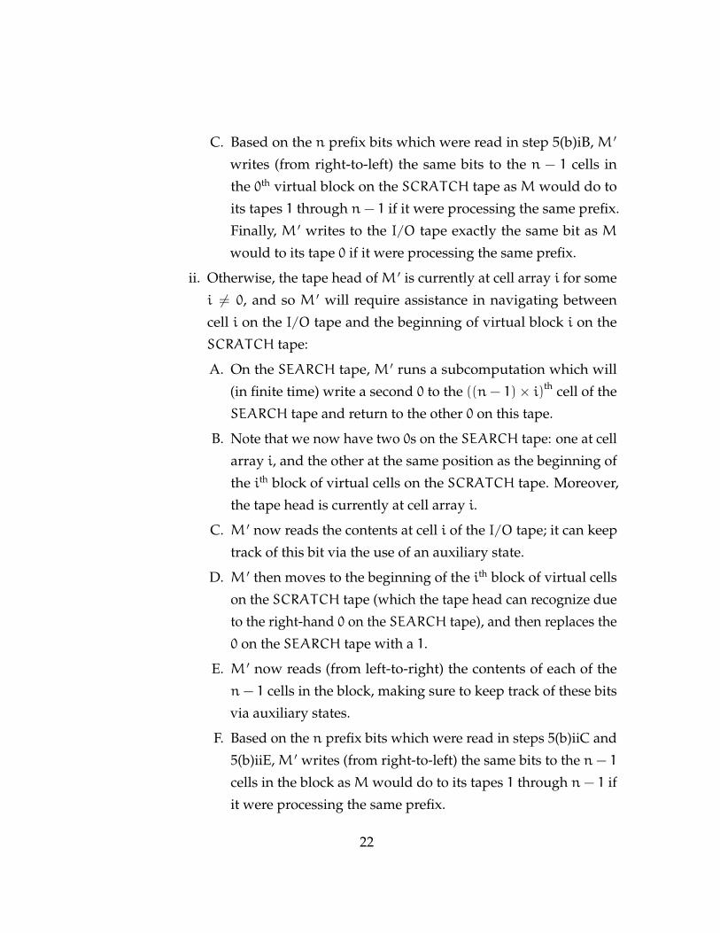
are intended to accomplish roughly the following purposes (see Figure 2.1 on page

24 for an illustration):

• The I/O tape is used to receive the initial program input, and will eventually

function exactly like the output tape (tape 0) ofM.

• The cells of the SCRATCH tape will be used to house “virtual” copies of

tapes 1 through n − 1 from M. More specifically, the block of SCRATCH

tape cells 0 through n− 2 will be used to represent cell 0 of tapes 1 through

n − 1 from M, the block of SCRATCH tape cells n − 1 through 2n − 3 will

be used to represent cell 1 of tapes 1 through n− 1 fromM, etc.

• The SEARCH tape will host a subcomputation that assists the tape head in

navigating between the I/O tape and the corresponding virtual cells on the

SCRATCH tape. More specifically, this subcomputation will, starting from a

SEARCH tape consisting of all 1s, excepting a single 0 in cell i (where i 6= 0),

write a second 0 to the ((n− 1)× i)th cell of the SEARCH tape and return to

the original 0 on said tape. We will explain the use of this subcomputation

20

in the course of describing our algorithm.

We now provide a “lower-level” sketch of what the instructions ofM ′ should

accomplish:

1. The initial input x ∈ X is passed to the I/O tape.

2. In the first ω steps of execution, M ′ transfers (i.e., deletes and copies), for

successive values of i > 0, the contents of I/O cell i to SCRATCH cell

i× (n− 1) + 1. At the same time, it also fills the SEARCH tape with 1s.

3. At this point in the computation, the I/O tape is blank, a virtual copy of

tape 1 (input tape) fromM lies on the SCRATCH tape, the SEARCH tape is

completely full of 1s, andM ′ is in the LIMIT state.

4. At this first LIMIT state,M ′ now transitions to the initial state forM.

5. For the remainder of its run-time, M ′ will repeatedly simulate successor

steps ofM, each simulation of which will only require finitely many actual

steps of computation. More precisely, if the tape head lies at cell array i at

the start of the execution of such a simulated step:

(a) Note that at the start of this step,M ′ has all 1s on its SEARCH tape.

(b) M ′ writes a 0 to the SEARCH tape and then determines if i = 0 (i.e., the

tape head is on the left-hand side). M ′ can do so by trying to move the

tape head one cell to the left. As there is currently only one 0 on the

SEARCH tape, the tape head will then be reading a 0 on the SEARCH

tape if and only if i = 0.

i. If i = 0,M ′ does the following:

A. M ′ replaces the 0 on the SEARCH tape with a 1.

B. M ′ reads the contents of the OUTPUT tape and then reads

(from left-to-right) the n− 1 bits in the 0th virtual block on the

SCRATCH tape; it can keep track of the values of these n bits

by the use of auxiliary states.

21

C. Based on the n prefix bits which were read in step 5(b)iB, M ′

writes (from right-to-left) the same bits to the n − 1 cells in

the 0th virtual block on the SCRATCH tape as M would do to

its tapes 1 through n− 1 if it were processing the same prefix.

Finally, M ′ writes to the I/O tape exactly the same bit as M

would to its tape 0 if it were processing the same prefix.

ii. Otherwise, the tape head ofM ′ is currently at cell array i for some

i 6= 0, and so M ′ will require assistance in navigating between

cell i on the I/O tape and the beginning of virtual block i on the

SCRATCH tape:

A. On the SEARCH tape, M ′ runs a subcomputation which will

(in finite time) write a second 0 to the ((n− 1)× i)th cell of the

SEARCH tape and return to the other 0 on this tape.

B. Note that we now have two 0s on the SEARCH tape: one at cell

array i, and the other at the same position as the beginning of

the ith block of virtual cells on the SCRATCH tape. Moreover,

the tape head is currently at cell array i.

C. M ′ now reads the contents at cell i of the I/O tape; it can keep

track of this bit via the use of an auxiliary state.

D. M ′ then moves to the beginning of the ith block of virtual cells

on the SCRATCH tape (which the tape head can recognize due

to the right-hand 0 on the SEARCH tape), and then replaces the

0 on the SEARCH tape with a 1.

E. M ′ now reads (from left-to-right) the contents of each of the

n− 1 cells in the block, making sure to keep track of these bits

via auxiliary states.

F. Based on the n prefix bits which were read in steps 5(b)iiC and

5(b)iiE,M ′ writes (from right-to-left) the same bits to the n− 1

cells in the block asMwould do to its tapes 1 through n− 1 if

it were processing the same prefix.

22

G. M ′moves the tape head back to cell array i (which the tape head

can recognize due to the single 0which remains on the SEARCH

tape) and writes to the I/O tape exactly whatMwould do on

its tape 0 if it were processing the prefix from steps 5(b)iiC and

5(b)iiE. It then replaces the 0 on the SEARCH tape with a 1.

(c) Note that the tape head is now back at cell array i.

(d) M ′ then moves the tape head left or right as according to whatMwould

do if it were processing the prefix from step 5(b)iB (if i = 0) or steps

5(b)iiC and 5(b)iiE (if i 6= 0).

(e) Finally,M ′ transitions to the same stateMwould if it were processing

the prefix from step 5(b)iB (if i = 0) or steps 5(b)iiC and 5(b)iiE (if i 6= 0).

6. Note that at limit stages, a 1 will have appeared unboundedly often in every

cell of the SEARCH tape, thus ensuring that all the SEARCH tape cells will

now contain a 1 at this stage of the computation. Thus, our SEARCH tape

subcomputation will function properly at all subsequent iterations of step 5.

7. If at any point M ′ enters its HALT state, it returns the contents of its I/O

tape.

Note that at the end of each simulated successor step, the contents of each cell

on the I/O and SCRATCH tapes ofM ′ are exactly what those of the corresponding

cells forMwould be at the same point in the computation. Thus, as each simulated

successor step requires only finitely many steps ofM ′ computation, everyω steps

of the computation ofM ′ (beyond the initialω steps) is a faithful rendition ofω

steps of the computation ofM; more precisely, with every passage ofω steps of

M ′ computation, the contents of the I/O tape ofM ′ are exactly what the contents

of tape 0 (output tape) ofM would be at the same moment in time. Thus, as steps

5e and 7 above ensure thatM ′ andM halt on precisely the same inputs x ∈ X, it

follows thatM ′ infinite-time-computes f(x), as desired.

The following scholium to our proof of the n > 3 case of Theorem 2.2.1 will

then immediately establish Theorem 2.2.2:

23

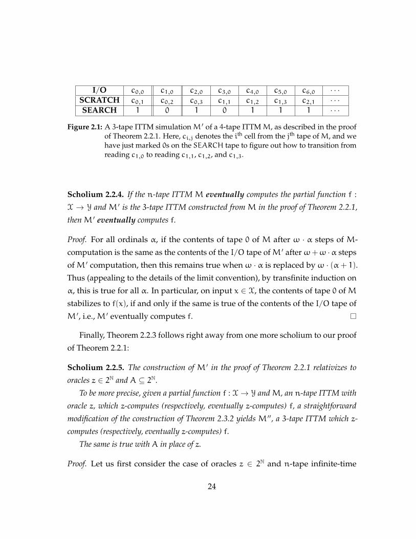
I/O c0,0 c1,0 c2,0 c3,0 c4,0 c5,0 c6,0 · · ·SCRATCH c0,1 c0,2 c0,3 c1,1 c1,2 c1,3 c2,1 · · ·SEARCH 1 0 1 0 1 1 1 · · ·

Figure 2.1: A 3-tape ITTM simulationM ′ of a 4-tape ITTMM, as described in the proofof Theorem 2.2.1. Here, ci,j denotes the ith cell from the jth tape ofM, and wehave just marked 0s on the SEARCH tape to figure out how to transition fromreading c1,0 to reading c1,1, c1,2, and c1,3.

Scholium 2.2.4. If the n-tape ITTM M eventually computes the partial function f :

X → Y and M ′ is the 3-tape ITTM constructed from M in the proof of Theorem 2.2.1,

thenM ′ eventually computes f.

Proof. For all ordinals α, if the contents of tape 0 of M after ω · α steps of M-

computation is the same as the contents of the I/O tape ofM ′ afterω+ω ·α steps

ofM ′ computation, then this remains true whenω · α is replaced byω · (α+ 1).

Thus (appealing to the details of the limit convention), by transfinite induction on

α, this is true for all α. In particular, on input x ∈ X, the contents of tape 0 of M

stabilizes to f(x), if and only if the same is true of the contents of the I/O tape of

M ′, i.e.,M ′ eventually computes f.

Finally, Theorem 2.2.3 follows right away from one more scholium to our proof

of Theorem 2.2.1:

Scholium 2.2.5. The construction of M ′ in the proof of Theorem 2.2.1 relativizes to

oracles z ∈ 2N and A ⊆ 2N.

To be more precise, given a partial function f : X→ Y andM, an n-tape ITTM with

oracle z, which z-computes (respectively, eventually z-computes) f, a straightforward

modification of the construction of Theorem 2.3.2 yields M ′′, a 3-tape ITTM which z-

computes (respectively, eventually z-computes) f.

The same is true with A in place of z.

Proof. Let us first consider the case of oracles z ∈ 2N and n-tape infinite-time

24

z-computable partial functions f : X→ Y. Fix such a z, f, and an n-tape ITTMM

which z-computes f.

LetM ′′ be the 3-tape ITTM with oracle z, which acts exactly as doesM ′ from

the proof of Theorem 2.2.1, save that at steps 5(b)iB and 5(b)iiC, M ′′ will also read

the contents at cell i of the ORACLE tape.

Based on the discussion at the end of the proof of Theorem 2.2.1, it is clear that

M ′′ will z-compute f.

Further, careful inspection of the proof of Scholium 2.2.4 reveals that if the exact

same construction is applied to an n-tape ITTM M which eventually z-computes

a partial function f : X→ Y, the resulting ITTMM ′′ will eventually z-compute f.

We now consider the case of oracles A ⊆ 2N and n-tape infinite-time A-

computable partial functions f : X → Y. Fix such a A, f, and an n-tape ITTM M

which A-computes f.

LetM ′′ be the 3-tape ITTM with oracle A, which acts exactly as doesM ′ from

the proof of Theorem 2.2.1, save that at steps 5(b)iB and 5(b)iiC, M ′′ will also read

a bit from the ORACLE tape and also check to see if the real on the ORACLE tape

lies in A. In addition, at steps 5(b)iC and 5(b)iiG, M ′′ also writes to cell i of the

ORACLE tape exactly whatMwould if it were processing the same prefix from

steps 5(b)iB (if i = 0) or 5(b)iiC and 5(b)iiE (if i 6= 0).Much as before, the discussion at the end of the proof of Theorem 2.2.1 shows

thatM ′′ will A-compute f.

A final analysis of Scholium 2.2.4 reveals that if the exact same construction

is applied to an n-tape ITTMMwhich eventually A-computes a partial function

f : X→ Y, the resulting ITTMM ′′ will eventually A-compute f.

2.3 Implementing Flags

In the setting of finite-time Turing machines, one can emulate an “if-then-else”

style of control statement by using specially designated groups of states to handle

the “then” and “else” subroutines separately.

25

Things are trickier when implementing infinite-time Turing machine programs,

as we have but one specially designated LIMIT state. Thus, if we wish to perform

two or more different kinds of subroutines during a limit stage of computation,

we must typically maintain some sort of “flag bits” on the left-hand side of the

tapes.

As this kind of bookkeeping can become prohibitively difficult to maintain,

we formulate an original extension of the ITTM model which has, as a primitive

construct, a finite collection of flag bits which do not lie on the tapes.

Definition 2.3.1. An n-tape ITTM with FLAGS M possesses exactly the same

hardware as a standard n-tape ITTM, save for the following adjustments:

• M is also assumed to have a fixed finite numberm ∈ N of “flag cells” F0, F1,

. . ., Fm−1. Like the standard tape cells, these flag cells can store 0s and 1s,

but unlike the tape cells, they can be instantaneously consulted and written

to at any point in the computation.

• All of the instruction prefixes and suffixes of M now also contain the sub-

string F0a0F1a1 · · · Fm−1am−1, where for every 0 6 i 6 m− 1, ai ∈ {0, 1}. In

a prefix, this substring intended to mean “The bits in F0, F1, . . ., Fm−1 are a0,

a1, . . ., am−1 (respectively),” while in a suffix, it means “Change the contents

of F0, F1, . . ., Fm−1 to a0, a1, . . ., am−1 (respectively).”

At successor stages, M will execute the instruction whose prefix applies to (1)

the bits which are currently being read by the tape head, (2) the bits which are

currently on the flags, and (3) the current state. The execution is carried out thusly:

1. The tape head will write the bits dictated by the suffix.

2. The contents of the flag cells will be changed to those specified in the suffix.

3. The tape head will move in the direction indicated by the suffix.

4. The current state will be changed to the one from the suffix.

Finally, upon reaching a limit stage of computation, the following occurs:

26

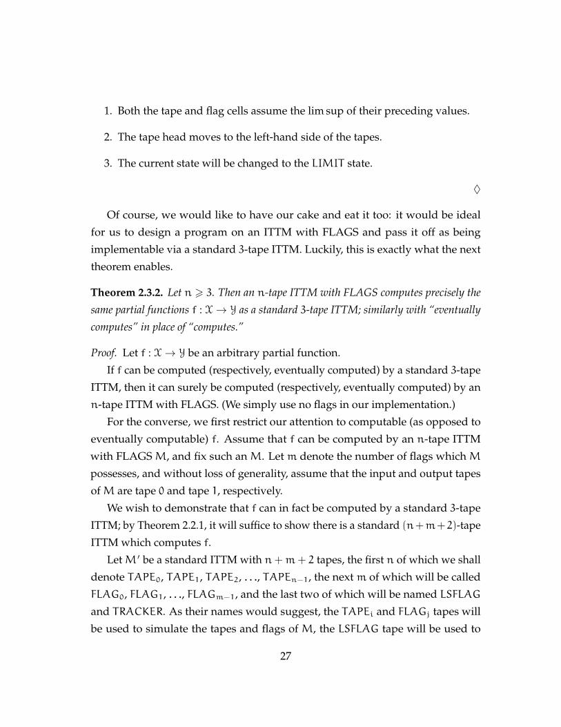
1. Both the tape and flag cells assume the lim sup of their preceding values.

2. The tape head moves to the left-hand side of the tapes.

3. The current state will be changed to the LIMIT state.

♦

Of course, we would like to have our cake and eat it too: it would be ideal

for us to design a program on an ITTM with FLAGS and pass it off as being

implementable via a standard 3-tape ITTM. Luckily, this is exactly what the next

theorem enables.

Theorem 2.3.2. Let n > 3. Then an n-tape ITTM with FLAGS computes precisely the

same partial functions f : X→ Y as a standard 3-tape ITTM; similarly with “eventually

computes” in place of “computes.”

Proof. Let f : X→ Y be an arbitrary partial function.

If f can be computed (respectively, eventually computed) by a standard 3-tape

ITTM, then it can surely be computed (respectively, eventually computed) by an

n-tape ITTM with FLAGS. (We simply use no flags in our implementation.)

For the converse, we first restrict our attention to computable (as opposed to

eventually computable) f. Assume that f can be computed by an n-tape ITTM

with FLAGS M, and fix such an M. Let m denote the number of flags which M

possesses, and without loss of generality, assume that the input and output tapes

ofM are tape 0 and tape 1, respectively.

We wish to demonstrate that f can in fact be computed by a standard 3-tape

ITTM; by Theorem 2.2.1, it will suffice to show there is a standard (n+m+2)-tape

ITTM which computes f.

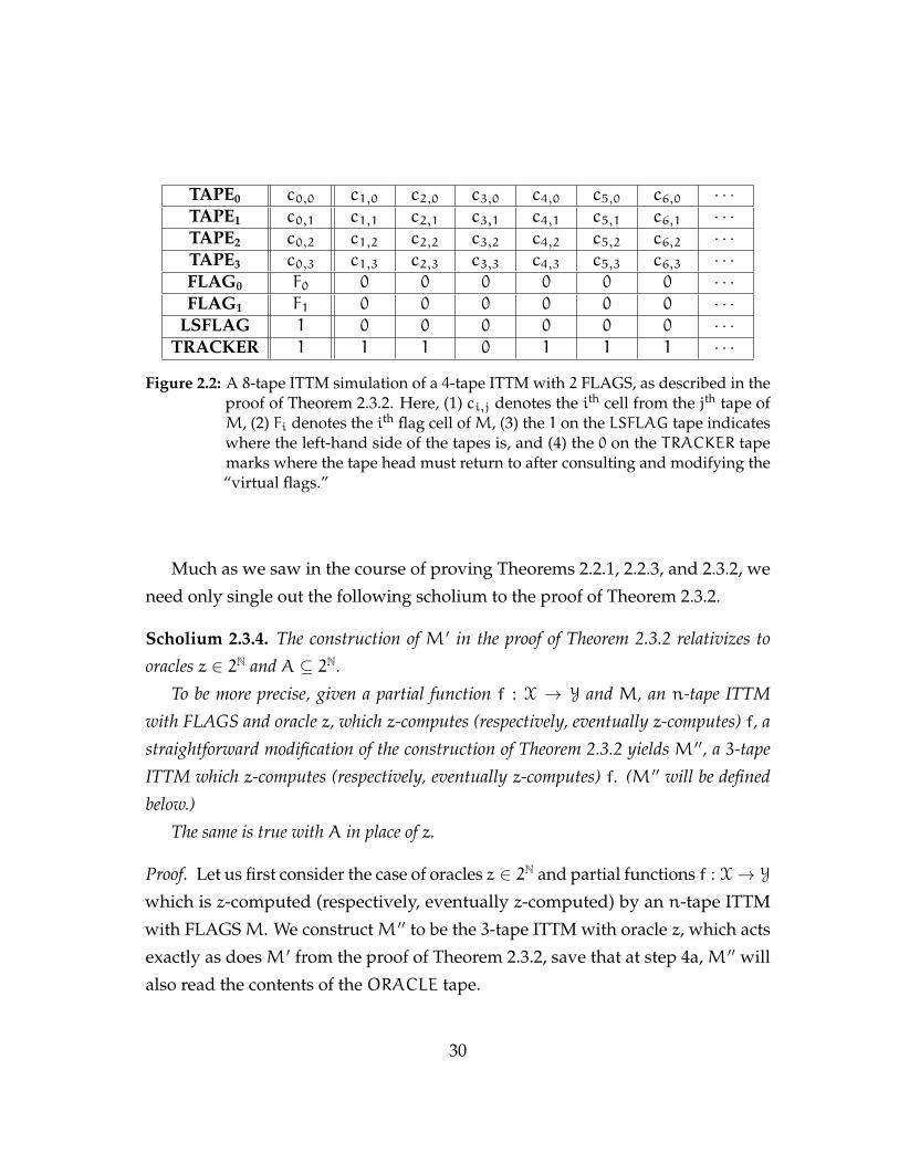
LetM ′ be a standard ITTM with n+m+ 2 tapes, the first n of which we shall

denote TAPE0, TAPE1, TAPE2, . . ., TAPEn−1, the next m of which will be called

FLAG0, FLAG1, . . ., FLAGm−1, and the last two of which will be named LSFLAG

and TRACKER. As their names would suggest, the TAPEi and FLAGj tapes will

be used to simulate the tapes and flags of M, the LSFLAG tape will be used to

27

mark the location of the left-hand side of the tapes, and the TRACKER tape will be

used to help the tape head return to the appropriate cell after a certain subroutine

in the algorithm outlined below (see Figure 2.2 on page 30 for an illustration).

We further stipulate thatM ′ has all of the states thatM does, as well as some

auxiliary states which will be employed when we wish to check or modify the

“virtual flags” on the FLAGj tapes.

Let us now indicate a “lower-level” sketch of what the instructions of M ′

should accomplish:

1. The initial input x ∈ X is passed to the TAPE0 tape andM ′ writes a 1 to the

LSFLAG tape (thus marking where the left-hand side of the tapes lies).

2. Inωmany steps,M ′ writes a 1 to every cell on the TRACKER tape, and then

enters the LIMIT state for the first time.

3. At the first visit to the LIMIT state,M ′ transitions to the initial state ofM.

4. For the remainder of the computation, M ′ repeatedly simulates successor

steps ofM (each in finitely many steps of actual computation) as follows:

(a) M ′ reads the bits on TAPE0, TAPE1, TAPE2, . . ., TAPEn−1 and writes a

0 to the TRACKER tape.

(b) Using auxiliary states to keep track of what was just read, M ′ moves

its tape head to the left-hand side of the tapes (which it can recognize

thanks to the 1 on cell 0 of the LSFLAG tape) and then read the bits on

FLAG0, FLAG1, . . ., FLAGm−1.

(c) Based on all of the bits that have been read in steps 4a and 4b, M ′

can then modify FLAG0, FLAG1, . . ., FLAGm−1 exactly as the relevant

instruction forMwould prescribe, and then move its tape head to right

until it encounters a 0 on the TRACKER tape, which it now replaces

with a 1. At this point, the tape head will then write to TAPE0, TAPE1,

TAPE2, . . ., TAPEn−1 exactly what M would do when confronted with

the prefix bits from steps 4a and 4b.

28

(d) M ′ then moves the tape head left or right as according to whatMwould

do if it were processing the prefix from steps 4a and 4b.

(e) Finally,M ′ transitions to the same stateMwould if it were processing

the prefix from steps 4a and 4b.

5. Note that at all limit stages of computation beyond the initial one, 1will have

occurred unboundedly often in all cells on the TRACKER tape, thus ensuring

that the TRACKER tape has reset to the necessary all-1s configuration needed

for successful execution of step 4.

6. If at any pointM ′ enters its HALT state, it returns the contents of its TAPE1tape.

Much as in the proof of Theorem 2.2.1, every block ofω steps of the computa-

tion ofM ′ is a faithful rendition ofω steps of the computation ofM; more precisely,

with every passage ofω steps ofM ′ computation, the contents of the TAPE1 tape

ofM ′ are exactly what the contents of tape 1 (output tape) ofMwould be at the

same moment in time. Thus, as steps 4e and 6 above ensure thatM ′ andM halt

on precisely the same inputs x ∈ X, it follows thatM ′ infinite-time-computes f(x),

as desired.

It remains to address case of eventually computable f, but this is straightfor-

ward: similar observations as those in the proof of Theorem 2.2.2 show that if f

is eventually computable by an n-tape ITTM with FLAGS M, the same kind of

ITTMM ′ as above will eventually compute f.

Just as we would hope, if we relativize Definition 2.3.1 in the natural way,

Theorem 2.3.2 then admits a nice relativization.

Theorem 2.3.3. Let n > 3, and z ∈ 2N. Then an n-tape ITTM with FLAGS z-computes

(and eventually z-computes) precisely the same partial functions f : X→ Y as a standard

3-tape ITTM.

The same is true with A ⊆ 2N in place of z ∈ 2N.

29

TAPE0 c0,0 c1,0 c2,0 c3,0 c4,0 c5,0 c6,0 · · ·TAPE1 c0,1 c1,1 c2,1 c3,1 c4,1 c5,1 c6,1 · · ·TAPE2 c0,2 c1,2 c2,2 c3,2 c4,2 c5,2 c6,2 · · ·TAPE3 c0,3 c1,3 c2,3 c3,3 c4,3 c5,3 c6,3 · · ·FLAG0 F0 0 0 0 0 0 0 · · ·FLAG1 F1 0 0 0 0 0 0 · · ·

LSFLAG 1 0 0 0 0 0 0 · · ·TRACKER 1 1 1 0 1 1 1 · · ·

Figure 2.2: A 8-tape ITTM simulation of a 4-tape ITTM with 2 FLAGS, as described in theproof of Theorem 2.3.2. Here, (1) ci,j denotes the ith cell from the jth tape ofM, (2) Fi denotes the ith flag cell ofM, (3) the 1 on the LSFLAG tape indicateswhere the left-hand side of the tapes is, and (4) the 0 on the TRACKER tapemarks where the tape head must return to after consulting and modifying the“virtual flags.”

Much as we saw in the course of proving Theorems 2.2.1, 2.2.3, and 2.3.2, we

need only single out the following scholium to the proof of Theorem 2.3.2.

Scholium 2.3.4. The construction of M ′ in the proof of Theorem 2.3.2 relativizes to

oracles z ∈ 2N and A ⊆ 2N.

To be more precise, given a partial function f : X → Y and M, an n-tape ITTM

with FLAGS and oracle z, which z-computes (respectively, eventually z-computes) f, a

straightforward modification of the construction of Theorem 2.3.2 yields M ′′, a 3-tape

ITTM which z-computes (respectively, eventually z-computes) f. (M ′′ will be defined

below.)

The same is true with A in place of z.

Proof. Let us first consider the case of oracles z ∈ 2N and partial functions f : X→ Y

which is z-computed (respectively, eventually z-computed) by an n-tape ITTM

with FLAGSM. We constructM ′′ to be the 3-tape ITTM with oracle z, which acts

exactly as doesM ′ from the proof of Theorem 2.3.2, save that at step 4a, M ′′ will

also read the contents of the ORACLE tape.

30

Reflecting on the end of the proof of Theorem 2.3.2 makes it clear thatM ′′ will

z-compute (respectively, eventually z-compute) f.

We now consider the case of oracles A ⊆ 2N and an n-tape ITTM with FLAGS

M which acts exactly as does M ′ from the proof of Theorem, 2.3.2 does, save that

at step 4a,M ′′ will also read a bit from the ORACLE tape and check to see if the

real on the ORACLE tape lies in A. In addition, at step 4c, M ′′ also writes to the

ORACLE tape exactly what M would if it were processing the prefix bits from

steps 4a and 4b.

A second and final reflection on the proof of Theorem 2.3.2 reveals that M ′′

will A-compute (respectively, eventually A-compute) f.

31

Chapter 3

A Busy Beaver Problem for

Infinite-Time Turing Machines

In this chapter, we formulate two different extensions for the Σ busy beaver

function, one to the setting of infinite-time computable functions, and the other to

that of infinite-time eventually computable functions. We will see that the analogue

of Rado’s central result in [Rad62] holds for both extensions (see Theorem 3.2.2),

and as corollaries thereto, we will be able to provide strikingly large asymptotic

lower bounds for each (via Theorems 3.2.4, 3.2.7, and 3.2.11), as well as conduct a

thorough analysis of their infinite-time degrees (as summarized in Theorems 3.3.3

and 3.3.8).

In handling all of this business, we will have our first exposure to how infinite-

time computation manifests its power in impressive ways, even when tethered to

the setting of type 0 spaces; this motif will reemerge in the course of Chapter 4.

Note. Throughout this chapter, ϕp (respectively, ϕep) shall be shorthand for ϕ(N,N)p

(respectively, ϕe,(N,N)p ). 4

32

3.1 Extending Σ to Infinite-Time Turing Machines

We first define the classical busy beaver function Σ. To that end, we make the

following auxiliary definitions.

Definition 3.1.1. For every index p ∈ N of a finite- or infinite-time Turing machine

program, we let states (p) denote its number of non-halting, non-limit states. ♦

Definition 3.1.2. Let BB-n = {p ∈ N states (p) = n and ft-ϕp(0) is defined}. ♦

Put in words, BB-n is the set of all indices of finite-time Turing machine

programs with n non-halting states which, upon starting with a blank INPUT

tape, ultimately halt with an OUTPUT tape which has (necessarily) finite number

of 1s on its left-hand side, and 0s elsewhere.

With these auxiliary definitions, we can succinctly define Σ.

Definition 3.1.3. Let Σ(n) = maxp∈BB-n

ft-ϕp(0). ♦

In other words, Σ(n) is the largest consecutive run of 1s which can appear on

the left-hand side of the OUTPUT tape (with 0s elsewhere) of some finite-time

Turing machine with index p ∈ BB-n which was executed with a blank INPUT

tape, and which has just halted.

It is also worth noting that the definition we have given here differs from Rado’s

original formulation in one aspect: Rado instead defined Σ(n) to be the largest

number of (not necessarily consecutive) 1s which can appear on an OUTPUT tape

as described in the previous paragraph. We have opted to use the definition from

the works of [Her08] and others for the sake of keeping our subsequent definitions

and related proofs concise.

We can readily extend Σ to the setting of both halting and stabilizing infinite-

time Turing machines by defining appropriate generalizations of BB-n.

Definition 3.1.4. Let

BB∞-n = {p ∈ N states (p) = n and ϕp(0) is defined} and

BBe∞-n ={p ∈ N states (p) = n andϕep(0) is defined

}.

33

♦

Viewed another way, BB∞-n (respectively, BBe∞-n) is the set of all indices of

infinite-time Turing machine programs with n non-halting, non-limit states which,

upon starting with a blank INPUT tape, ultimately halt (respectively, stabilize)

with an OUTPUT tape which has finitely many 1s on its left-hand side, and 0s

elsewhere.

Definition 3.1.5. In analogy with Definition 3.1.3, we now define

Σ∞(n) = maxp∈BB∞-n

ϕp(0) and Σe∞(n) = maxp∈BBe∞-n

ϕep(0).

♦

Remark. Note that Σ∞(n) and Σe∞(n) are necessarily finite, as since we are working

in a type 0 setting, our definitions of BB∞-n and BBe∞-n rule out indices p of

ITTMs which, upon starting with blank tape, leave infinitely many ones on the

OUTPUT tape and then halt. 4

3.2 Some Domination Results for Σ∞ and Σe∞Our aim in this section is to extend Rado’s famous domination result for Σ (stated

below) to Σ∞ and Σe∞, and then use it to establish the promised asymptotic lower

bounds of Σ∞ and Σe∞.

Theorem 3.2.1 (Rado). If f : N → N is a total finite-time computable function, then

Σ(n) >∗ f(n).

We now state and prove our first main theorem, which is an exact analogue

of Rado’s result for finite-time Turing machines. In doing so, we achieve our first

significant payoff for our work in Section 2.1.

Theorem 3.2.2. If f : N→ N is a total infinite-time computable function, then Σ∞(n) >∗f(n). Similarly, if f : N→ N is a total infinite-time eventually computable function, then

Σe∞(n) >∗ f(n).34

Proof. We will be content to prove the first half of the theorem, as the other half

may be proven mutatis mutandis.

To that end, let f : N→ N be a total infinite-time computable function. Follow-

ing Rado, we define the function F : N→ N by

F(k) =

k∑i=0

[f(i) + i2

].

This function is evidently infinite-time computable via Theorems 2.1.1 and 2.1.3,

as it can be defined by the following primitive recursion:

F(0) = f(0)

F(k+ 1) = F(k) + f(k+ 1) + (k+ 1)2.

As F is infinite-time computable, we may fix a 3-tape ITTMMwhich computes

F ◦ F. Let S denote the number of non-halting, non-limit states whichM possesses.

We devote the rest of the proof to showing that Σ∞(k+ 1+ S) >∗ f(k+ 1+ S);this clearly suffices since we can then take n = k+ 1+ S.

To do so, we first construct a family {Mk k ∈ N} of infinite-time Turing ma-

chines such that for every k ∈ N, (1)Mk possesses k+ 1+ S non-halting, non-limit

states and (2) starting from a blank INPUT tape,Mk ultimately writes the value

of F(F(k)) to its OUTPUT tape and then halts.

Given an arbitrary k ∈ N, we designMk according to the following specifica-

tions:

1. Using k states, Mk writes a single 1 to the left-hand side of the SCRATCH

tape and also writes a string of k 1s to the INPUT tape.

2. In 1 additional state,Mk can return to the left-hand side of the tapes (which

it can recognize thanks to the 1 on the SCRATCH tape) and erase the 1 on

the SCRATCH tape.

3. Finally, using S states,Mk can write the value of F(F(k)) to itsOUTPUT tape

and then halt.

35

With this construction handled, we next observe that for every k ∈ N, the

following inequalities hold:

F(k) > f(k), as F(k) =k∑i=0

[f(i) + i2

]> f(k) + k2 > f(k). (3.1)

F(k) > k2, as F(k) =k∑i=0

[f(i) + i2

]> f(k) + k2 > k2. (3.2)

F(k+ 1) > F(k), as F(k+ 1) = F(k) + f(k+ 1) + (k+ 1)2 > F(k). (3.3)

Let k ∈ N be arbitrary but fixed. Then it follows directly from the construction

ofMk that

Σ∞(k+ 1+ S) > F(F(k)). (3.4)

Moreover, as it is clear that k2 >∗ k+ 1+ S, it follows from inequality (3.2) that

F(k) >∗ k + 1 + S. Thus, as F is strictly increasing (by inequality (3.3)), we have

that

F(F(k)) >∗ F(k+ 1+ S). (3.5)

Combining (3.4) and (3.5) then yields

Σ∞(k+ 1+ S) >∗ F(k+ 1+ S). (3.6)

Thus, as F(k+ 1+ S) > f(k+ 1+ S) (by inequality (3.1)), it follows from (3.6)

that Σ∞(k+ 1+ S) >∗ f(k+ 1+ S), as we sought to verify.

Theorem 3.2.2 has the following immediate corollary.

Corollary 3.2.3. Σ∞ (respectively, Σe∞) is not infinite-time computable (respectively,

eventually computable).

The next theorem shows that the growth rate of our busy beaver functions are

interrelated in precisely the fashion we would expect.

Theorem 3.2.4. Σe∞(n) >∗ Σ∞(n) >∗ Σ(n).

36

Proof. By Theorem 3.2.2, it suffices to show that Σ (respectively, Σ∞) is infinite-time

computable (respectively, eventually computable).

In [HL00], Hamkins and Lewis describe an ITTM M which simultaneously

simulates, in everyω steps of actual computation,ω steps of each computation

ϕp(0).

This machine makes it easy to establish the infinite-time computability of Σ:

for a given n ∈ N, we executeω steps ofM and then systematically check which

computations ϕp(0) have (1) halted with unary output and (2) states (p) = n; we

then return the largest unary output among such computations.

With a little more care, M can also be used to prove that Σ∞ is infinite-time

eventually computable: given n ∈ N, we execute M and maintain a guess for

Σ∞(n) on a separate tape. Every time a computationϕp(0) halts, we check to see if

(1) its output is unary, (2) states (p) = n, and (3) its output surpasses our current

guess; if these three conditions are met, we update our guess appropriately. After

all of the members of BB∞-n have halted, our guess will have stabilized to the

correct value for Σ∞.

For the remainder of this section, we focus on finding asymptotic lower

bounds for Σ∞. Our first order of business here is to exhibit suitable choices

of Σ-pointclasses Γ such that Σ∞ dominates the entire class of Γ -recursive func-

tions.

Note. The reader who is unfamiliar with the notions of a Σ-pointclass and Γ -

recursive function need not worry, as in view of Lemma 3.2.5, we do not require

the formal definitions thereof; for the purpose of motivation, we opt to give infor-

mal definitions here and refer the still-curious reader to Moschovakis’ excellent

treatment in [Mos09].

Roughly speaking, a Σ-pointclass Γ is a pointclass which is closed under a

certain small collection of logical connectives and quantifications (including, but

not limited to, conjunction, disjunction, and ∃(n < ω)). Moreover, a total function

f : N→ N is Γ -recursive precisely when a certain effective presentation of its graph

lies in Γ . 4

37

The following lemma of Moschovakis, as stated in [Mos09], gives a useful

characterization of certain kinds of Γ -recursive functions.

Lemma 3.2.5 (Moschovakis). Let Γ be a Σ-pointclass and f : X→ N be total.

Then f is Γ -recursive if and only if Graph (f) ∈ Γ .

Definition 3.2.6. Let sD denote the Σ-pointclass of infinite-time semi-decidable

sets. ♦

Remark. That sD is a Σ-pointclass follows from the results of [HL00] and the formal

definition of Σ-pointclasses, as given in [Mos09]. 4

Theorem 3.2.7. If f : N→ N is sD-recursive, then Σ∞(n) >∗ f(n).Proof. Let f : N→ N be sD-recursive.

By Theorem 3.2.2, it suffices to demonstrate that f is infinite-time computable.

Observe that by Lemma 3.2.5, Graph (f) is infinite-time semi-decidable. Thus,

its partial characteristic function pcGraph(f)(n,m) is infinite-time computable.

Let n ∈ N be arbitrary but fixed. We wish to infinite-time-compute f(n).

In [HL00], Hamkins and Lewis describe an ITTM which can simulate the

computations pcGraph(f)(n,m) for all values of m ∈ N simultaneously. When

one of these computations halts (which will ultimately happen, as f, being sD-

recursive, is total), we simply return the corresponding value of m (which of

course equals f(n)) and halt.

Remark. This proof gives a subtle affirmation of one of the benefits of working in

type 0 spaces. Unlike in finite-time computability, one cannot in general conclude

that a function f : X → Y is infinite-time computable solely on the basis of the

semi-decidability of its graph. In fact, Hamkins and Lewis’ famous Lost Melody

Theorem exhibits a constant function whose graph is infinite-time decidable, but

which is nevertheless not infinite-time computable (see [HL00])! 4

As an easy consequence of Theorem 3.2.7, we have the following corollary.

Corollary 3.2.8. If f : N→ N is Π11-recursive, then Σ∞(n) >∗ f(n).38

Proof. Simply observe that Π11 ⊆ sD and apply Theorem 3.2.7.

The last result of this section has an amusing connection to (mathematical)

popular culture, as humorously recounted in [Ray].

During MIT’s 2007 Independent Activity Period, the philosophy department

staged a so-called “large number battle” between its faculty members Rayo and

Elga. Subject to a modest set of rules, each man in turned named progressively

larger numbers, until Elga finally conceded defeat at the hands of the following

entry of Rayo’s:

The smallest number bigger than any finite number named by

an expression in the language of first-order set theory with a googol

symbols or less.

Of course, there is nothing special about the number “googol” here; relaxing

this number gives us the following function, which has been considered exten-

sively by the online Googology community. (“Googology” is the hobbyist study

of large numbers and fast-growing functions.)

Definition 3.2.9. For every n ∈ N, let Rayo (n) denote the smallest natural number

which is not definable via a formula in first-order set theory which possesses at

most n symbols. ♦

There is little hope that Σ∞ or Σe∞ could eventually dominate Rayo; after all, it

is not too hard to see that one could express predicates such as “∃n such that n ∈N and Σ∞(n) = k” and “∃n such that n ∈ N and Σe∞(n) = k” in first-order set

theory.

The following definition will “even the score.”

Definition 3.2.10. For every n ∈ N, letWeakRayo (n) denote the smallest natural

number which is not definable via a formula in first-order arithmetic which

possesses at most n symbols. ♦

39

We now show that, while Σ∞ likely does not eventually dominate Rayo, it

does eventually dominateWeakRayo, and hence in some sense, all of first-order

arithmetic.

Theorem 3.2.11. Σ∞(n) >∗ WeakRayo (n)Proof. Because it is well-known that all arithmetically definable formulas are Π11,

we can immediately appeal to Corollary 3.2.8.

3.3 The Infinite-Time Degree of Σ∞ and Σe∞To cap off this chapter, we characterize the infinite-time degree of Σ∞ and derive

two equally intriguing possibilities for that of Σe∞.

In their paper [HL02], Hamkins and Lewis showed that the natural infinite-

time analogues of Post’s Problem had both positive and negative solutions, de-

pending upon the type of oracle being considered.

Since Graph (Σ∞) is coded by a single real, the negative solution for oracles

which are single reals is the relevant result for us:

Theorem 3.3.1 (Hamkins and Lewis). There are no reals z such that 0 <∞ z <∞ 0O.

To prove Theorem 3.3.3, we will require the following lemma, which once more

exploits the fact that we are working in a type 0 setting.

Lemma 3.3.2. Let f : N→ N. If Graph (f) is infinite-time decidable (respectively, even-

tually decidable), then f is infinite-time computable (respectively, eventually computable).

Proof. Let f : N → N have an infinite-time decidable (respectively, eventually

decidable) graph. Then by Theorem 2.1.4,

f(n) ' µm ((n,m) ∈ Graph (f))

is infinite-time computable (respectively, eventually computable).

With both of these results in hand, we can now resolve the infinite-time degree

of Σ∞.

40

Theorem 3.3.3. Graph (Σ∞) ≡∞ 0O.

Proof. First note that 0 6∞ Graph (Σ∞), as 0 is of course decidable even without

the use of Graph (Σ∞) as an oracle. Moreover, 0 <∞ Graph (Σ∞), by Lemma 3.3.2

(since Σ∞ is not infinite-time computable).

We next verify that Graph (Σ∞) 6∞ 0O. To this end, it suffices to show that

Σ∞ is infinite-time 0O-computable: given 0O as an oracle and an arbitrary n ∈ N,

we can, just as in the proof of Theorem 3.2.4, run an ITTM which simulates

each computation ϕp(0) simultaneously. Further, as 0O encodes which indices

p correspond to halting computations with states (p) = n, we can wait until all

such computations ϕp(0) have halted and return the largest unary output from

among them.

Finally, as 0 <∞ Graph (Σ∞) 6∞ 0O, we must have Graph (Σ∞) ≡∞ 0O, lest

Theorem 3.3.1 be contradicted.

In order to conduct a similar investigation for Σe∞, we first summarize Hamkins

and Lewis’ characterization of the infinite-time eventually writable and acciden-

tally writable degrees in [HL02].

Definition 3.3.4. An infinite-time degree is said to be eventually writable (re-

spectively, accidentally writable) if it has an eventually writable (respectively,

accidentally writable) representative. ♦

In [HL02], Hamkins and Lewis constructed a “backbone sequence” of eventu-

ally writable degrees 〈0Oα α < ζ〉 by defining a transfinite iteration of the weak

jump. More concretely, they set 0O0 = 0 and 0Oα+1 =(0O

α)O, and for limit δ, they

took 0Oδ to be a certain type of “effective supremum” of the preceding degrees 0Oα

(α < δ).

Using Theorem 3.3.1 and a certain continuity property of the backbone se-

quence, Hamkins and Lewis showed that they had in fact exhausted all of the

eventually writable degrees:

Theorem 3.3.5 (Hamkins and Lewis). The eventually writable infinite-time degrees

are precisely those which lie on the backbone sequence 〈0Oα α < ζ〉.

41

For an encore, Hamkins and Lewis proved that the backbone sequence misses

but one accidentally writable degree. More precisely:

Theorem 3.3.6 (Hamkins and Lewis). The accidentally writable infinite-time degrees

are well-ordered by <∞ and have order type ζ + 1. In particular, there is a unique

accidentally writable infinite-time degree which is not eventually writable.

The preceding theorem motivates the following definition.

Definition 3.3.7. Let 0Oζ denote the maximal accidentally writable infinite-time

degree. ♦

With these preliminaries handled, we can narrow down the infinite-time degree

of Σe∞ to two potential alternatives.

Theorem 3.3.8. There are two possibilities for the infinite-time degree of Graph (Σe∞):1. Graph (Σe∞) ≡∞ 0Oζ .2. Graph (Σe∞) lies in an infinite-time degree with no accidentally writable represen-

tatives.

Proof. It suffices to show that Graph (Σe∞) is not infinite-time eventually writable,

as we would then have Graph (Σe∞) ≡∞ 0Oζ (if the degree of Graph (Σe∞) is ac-

cidentally writable) or that Graph (Σe∞) lies in an infinite-time degree with no

accidentally writable representatives (if the degree of Graph (Σe∞) is not acciden-

tally writable).

Assume to the contrary that Graph (Σe∞) is in fact infinite-time eventually

writable. Then Graph (Σe∞) is infinite-time eventually decidable: given an arbi-

trary input (n,m) ∈ N× N, we simply run an ITTMM which eventually writes a

code for Graph (Σe∞), and on a separate tape, we maintain a guess as to whether

or not (n,m) ∈ Graph (Σe∞); at limit stages, this guess will be updated based on

the current contents of M’s OUTPUT tape. As M’s OUTPUT tape stabilizes to a

code for Graph (Σe∞), our guess will ultimately stabilize to the correct answer.

42

We have now arrived at a contradiction: since Graph (Σe∞) is infinite-time

eventually decidable, we have that Σe∞ is infinite-time eventually computable

(by Lemma 3.3.2), which runs afoul of Corollary 3.2.3. The conclusion is that

Graph (Σe∞) is not eventually writable.

43

Chapter 4

A Fast-Growing Hierarchy Based on

Infinite-Time Turing Machines

We develop a fast-growing hierarchy that extends through all ordinals α < ζ (see

Definition 4.3.1), and indicate tiers which our busy beaver functions Σ∞ and Σe∞eventually dominate (via Corollaries 4.3.4 and 4.3.6 to Theorems 4.3.3 and 4.3.5).

In the course of designing this hierarchy, we will find it necessary to derive

sufficiently effective systems of ordinal notations for all ordinals up to ζ. We do so

by a natural refinement of Klev’s extension of Kleene’s O to the setting of infinite-

time Turing machines (as described in [Kle09]). The ease with which we will

be able to formulate these systems speaks volumes to the power of infinite-time

Turing machines in handling such affairs.

Note. Throughout this chapter, ϕp (respectively, ϕep) will once again be used as

shorthand for ϕ(N,N)p (respectively, ϕe,(N,N)p ). 4

4.1 Review of Fast-Growing Hierarchies and Ordinal

Notation

Definition 4.1.1. Let δ be a countable limit ordinal. A fundamental sequence for δ

is a strictly increasingω-sequence of ordinals 〈 δ[n] n < ω 〉 such that limn→ω

δ[n] =

44

δ. ♦

Remark. It is an elementary fact from set theory that every countable limit ordinal

in fact possesses a fundamental sequence. 4

Definition 4.1.2. Let µ be a countable ordinal, and suppose further that fundamen-

tal sequences have been assigned to all limit ordinals δ < µ. Then the associated

fast-growing hierarchy of functions fα : N → N for all α < µ is defined by

transfinite recursion as follows:

f0(n) = n+ 1

fα+1(n) = fnα(n)

fδ(n) = fδ[n](n),

where fnα(n) denotes the n-fold iterate of fα(n). ♦

From the definition, it is clear that the primary challenge of constructing a

fast-growing hierarchy up to some countable ordinal µ is describing a uniform

method of assigning fundamental sequences for all limit ordinals δ < µ. For the

purposes of proving Theorems 4.3.3 and 4.3.5, we will also find it necessary to find

a method which is not just uniform, but also, in a suitable sense, effective.

To obtain our desired assignment of fundamental sequences, we will first

obtain an appropriate system of ordinal notations from the infinite-time analogues

of Kleene’s O.

Definition 4.1.3. Kleene’s O is the subset of N coding the least transitive binary

relation <O on N with the following properties:

1. 1 <O 2.

2. If n ∈ field (<O), then 2n ∈ field (<O).

3. For every p ∈ N: if ft-ϕp is total and ft-ϕp(n) <O ft-ϕp(n+ 1) for all n ∈ N,

then for every n ∈ N, ft-ϕp(n) <O 3 · 5p.

♦

45

This classical definition generalizes easily to the following:

Definition 4.1.4. Let F = { Fp p ∈ N } be a family of functions.

Then OF, the analogue of Kleene’s O for F, is the subset of N coding the least

transitive binary relation <OF on N with the following properties:

1. 1 <OF 2.

2. If n ∈ field (<OF), then 2n ∈ field (<OF).

3. For every p ∈ N: if N ⊆ dom (Fp), Fp[N] ⊆ N, and Fp(n) <OF Fp(n + 1) for

all n ∈ N, then for every n ∈ N, Fp(n) <OF 3 · 5p.

♦

Note. In this notation, Kleene’s O corresponds to the case where our family F is

the set of all finite-time computable functions. 4

In addition to the classical definition of Kleene’s O, we will be chiefly interested

in two of its analogues from the setting of infinite-time Turing machines, as initially

studied by Klev in [Kle07]:

Definition 4.1.5. In the sequel, O+ will denote the analogue of Kleene’s O for the

infinite-time computable functions, and similarly, O++ shall denote the analogue

of Kleene’s O for the infinite-time eventually computable functions. ♦

The next definition indicates how a notation for an ordinal α arises from an

analogue of Kleene’s O.

Definition 4.1.6. Let F = { Fp p ∈ N } be a family of functions.

We say thatn ∈ field (<OF) is an OF-notation for the ordinalα if the collection

{ k ∈ field (<OF) k <OF n } of<OF -predecessors of n is well-ordered by<OF with

order type α.

Under these circumstances, we write |n|OF = α. ♦

The following theorem shows that O, O+, and O++ are a rich source of ordinal

notations.

46

Theorem 4.1.7 (Kleene, Hamkins and Lewis, Klev). For easy reference, we collect the

following important facts about O, O+, and O++, as well as some associated ordinals:

1. O ( O+ ( O++.

2. ωCK1 < λ < ζ.

3. The relations <O, <O+ , and <O++ are rooted trees of heightωCK1 , λ, and ζ, respec-

tively. Consequently:

(a) All ordinals α < ωCK1 (respectively, α < λ, α < ζ) receive O-notations

(respectively, O+-notations, O++-notations).

(b) ωCK1 (respectively, λ, ζ) is the least ordinal to not receive an O-notation

(respectively, O+-notation, O++-notation).

4. Let F = { Fp p ∈ N } be the family of finite-time computable, infinite-time com-

putable, or infinite-time eventually computable functions. The following statements

hold for all ordinals α which receive OF-notations:

(a) α = 0 receives the unique OF-notation 1 (the root of the tree <OF).

(b) Successor ordinals α = α ′ + 1 receive OF-notations of the form 2k, where k is

any OF-notation of α ′.

(c) Finally, if δ is a limit ordinal, it receives OF-notations of the form 3 · 5p, where⟨|Fp(n)|OF n < ω

⟩is a fundamental sequence for δ.

4.2 Systems of Ordinal Notations up toωCK1 , λ, and ζ

In this section, we build up our desired system of ordinal notations “in layers” up

to heightsωCK1 , λ, and finally ζ.

While Theorem 4.1.7 indicates that O, O+, and O++ provide notations for all

ordinals up to ωCK1 , λ, and ζ, there is a fly in the ointment: as Klev explains in

[Kle07], only the finite ordinals receive unique notations. Consequently, we must

47

give some sort of uniform procedure for singling out unique notations for the

infinite ordinals; this is precisely what the following definition accomplishes.

Definition 4.2.1. The systems of Q-notations, Q+-notations, and Q++-notations are

defined as follows:

1. For every α < ωCK1 , the Q-notation for α is given by

qα = the least O-notation for α.

For q = qα, we also write |q|O = α, while if there is no α for which q = qα,

then |q|O is undefined.

2. For every α < λ, the Q+-notation for α is given by

q+α =

qα if α < ωCK1

the least O+-notation for α ifωCK1 6 α < λ.

For q = q+α , we also write |q|O+ = α, while if there is no α for which q = q+

α ,

then |q|O+ is undefined.

3. For every α < ζ, the Q++-notation for α is given by

q++α =

q+α if α < λ

the least O++-notation for α if λ 6 α < ζ..

For q = q++α , we also write |q|O++ = α, while if there is no α for which

q = q++α , then |q|O++ is undefined.

♦

We will demonstrate the effectiveness of the assignment of Q- and Q+-notations

in Theorem 4.2.6. Towards that goal, we state the following result from Hamkins

and Lewis’ [HL00], which can be proven via an elegant “double count-through”

argument.

48

Theorem 4.2.2 (Hamkins and Lewis). “x and y code isomorphic well-orderings on N”

is infinite-time decidable.

In addition, Klev established (in [Kle07]) that the relations <O and <O+ are

suitably effective for our purposes:

Theorem 4.2.3 (Klev). The real number codes for the relations <O and <O+ are writable

and eventually writable, respectively.

In a similar vein, the predicates “n ∈ field (<O)” and “n ∈ field (<O+)” are

infinite-time decidable and infinite-time eventually decidable, respectively.

The following technical lemma, concerning the rest function from Definition

1.1.5, will also be of use to us.

Lemma 4.2.4 (Hamkins and Lewis). The rest function is infinite-time computable.

Before we can finally provide the proof of Theorem 4.2.6, we first formulate

some auxiliary functions. Roughly speaking, given an arbitrary n ∈ O (respec-

tively, n ∈ O+, n ∈ O++), they return its corresponding Q-notation (respectively,

Q+-notation, Q++-notation).

Definition 4.2.5. Let qno : N→ N, qno+ : N→ N, and qno++ : N→ N be defined

as follows:

1. For every n ∈ N,

qno (n) =

q|n|Oif n has a Q-notation

undefined if n does not have a Q-notation.

2. For every n ∈ N,

qno+ (n) =

q|n|O+ if n has a Q+-notation

undefined if n does not have a Q+-notation.

49

3. For every n ∈ N,

qno++ (n) =

q|n|O++ if n has a Q++-notation

undefined if n does not have a Q++-notation.

♦

We have now covered enough preliminaries to prove Theorem 4.2.6.

Theorem 4.2.6. The Q-notations and Q+-notations, as well as the associated functions

qno and qno+, are effective in the following sense:

1. qno is infinite-time computable, and the predicate “n is a Q-notation” is partially

infinite-time decidable.

2. qno+ is infinite-time eventually computable, and the predicate “n is a Q+-notation”

is partially infinite-time eventually decidable.

Proof. Let R(x, y) be the predicate “x and y code isomorphic well-orderings on N.”

By Theorem 4.2.3, there exists an index p of an ITTM program which, upon

being given blank input, returns the code for <O and then halts; fix such a p. Then

for every n ∈ N,

qno (n) =

µo (o ∈ field (<O) and |n|O = |o|O) if n ∈ field (<O)

undefined if n 6∈ field (<O)

=

µo (o ∈ field (<O) and

R (rest (ϕp(0), n) , rest (ϕp(0), o))) if n ∈ field (<O)

undefined if n 6∈ field (<O).

Then by Theorems 2.1.1 and 2.1.4, as well as the infinite-time decidability of

R(x, y) and field (<O), qno is infinite-time computable.

To see that the Q-notations are partially infinite-time decidable, simply note

that

n is a Q-notation⇔ n = qno (n) ,

50

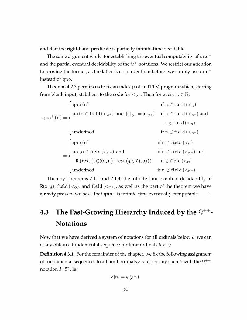
and that the right-hand predicate is partially infinite-time decidable.

The same argument works for establishing the eventual computability of qno+

and the partial eventual decidability of the Q+-notations. We restrict our attention

to proving the former, as the latter is no harder than before: we simply use qno+

instead of qno.

Theorem 4.2.3 permits us to fix an index p of an ITTM program which, starting

from blank input, stabilizes to the code for <O+ . Then for every n ∈ N,

qno+ (n) =

qno (n) if n ∈ field (<O)

µo (o ∈ field (<O+) and |n|O+ = |o|O+) if n ∈ field (<O+) and

n /∈ field (<O)

undefined if n 6∈ field (<O+)

=

qno (n) if n ∈ field (<O)

µo (o ∈ field (<O+) and if n ∈ field (<O+) and

R(rest

(ϕep(0), n

), rest

(ϕep(0), o

))) n /∈ field (<O)

undefined if n 6∈ field (<O+).

Then by Theorems 2.1.1 and 2.1.4, the infinite-time eventual decidability of

R(x, y), field (<O), and field (<O+), as well as the part of the theorem we have

already proven, we have that qno+ is infinite-time eventually computable.

4.3 The Fast-Growing Hierarchy Induced by the Q++-

Notations

Now that we have derived a system of notations for all ordinals below ζ, we can

easily obtain a fundamental sequence for limit ordinals δ < ζ:

Definition 4.3.1. For the remainder of the chapter, we fix the following assignment

of fundamental sequences to all limit ordinals δ < ζ: for any such δ with the Q++-

notation 3 · 5p, let

δ[n] = ϕep(n).

51

♦

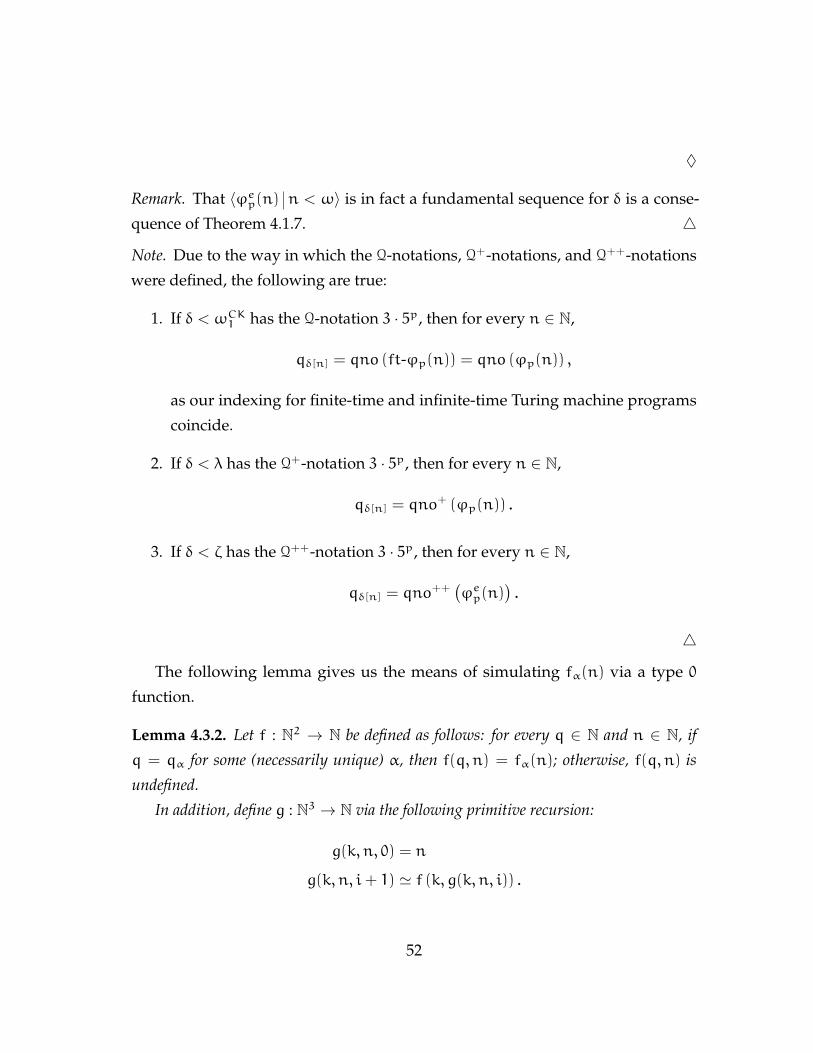
Remark. That 〈ϕep(n) n < ω〉 is in fact a fundamental sequence for δ is a conse-

quence of Theorem 4.1.7. 4

Note. Due to the way in which the Q-notations, Q+-notations, and Q++-notations

were defined, the following are true:

1. If δ < ωCK1 has the Q-notation 3 · 5p, then for every n ∈ N,

qδ[n] = qno (ft-ϕp(n)) = qno (ϕp(n)) ,

as our indexing for finite-time and infinite-time Turing machine programs

coincide.

2. If δ < λ has the Q+-notation 3 · 5p, then for every n ∈ N,

qδ[n] = qno+ (ϕp(n)) .

3. If δ < ζ has the Q++-notation 3 · 5p, then for every n ∈ N,

qδ[n] = qno++

(ϕep(n)

).

4

The following lemma gives us the means of simulating fα(n) via a type 0

function.

Lemma 4.3.2. Let f : N2 → N be defined as follows: for every q ∈ N and n ∈ N, if

q = qα for some (necessarily unique) α, then f(q, n) = fα(n); otherwise, f(q, n) is

undefined.

In addition, define g : N3 → N via the following primitive recursion:

g(k, n, 0) = n

g(k, n, i+ 1) ' f (k, g(k, n, i)) .

52

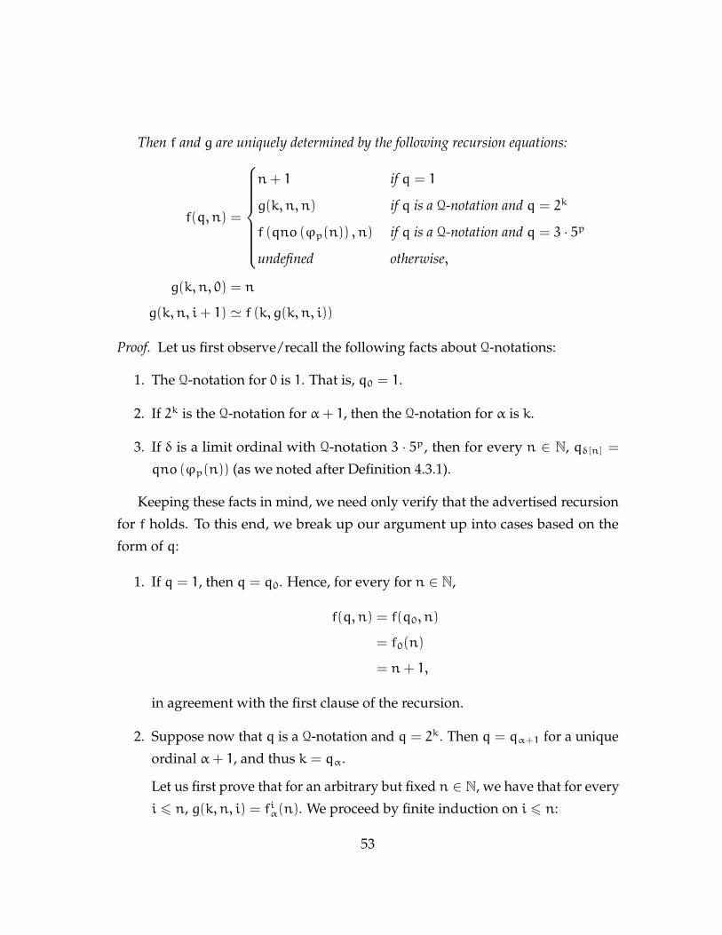
Then f and g are uniquely determined by the following recursion equations:

f(q, n) =

n+ 1 if q = 1

g(k, n, n) if q is a Q-notation and q = 2k

f (qno (ϕp(n)) , n) if q is a Q-notation and q = 3 · 5p

undefined otherwise,

g(k, n, 0) = n

g(k, n, i+ 1) ' f (k, g(k, n, i))

Proof. Let us first observe/recall the following facts about Q-notations:

1. The Q-notation for 0 is 1. That is, q0 = 1.

2. If 2k is the Q-notation for α+ 1, then the Q-notation for α is k.

3. If δ is a limit ordinal with Q-notation 3 · 5p, then for every n ∈ N, qδ[n] =

qno (ϕp(n)) (as we noted after Definition 4.3.1).

Keeping these facts in mind, we need only verify that the advertised recursion

for f holds. To this end, we break up our argument up into cases based on the

form of q:

1. If q = 1, then q = q0. Hence, for every for n ∈ N,

f(q, n) = f(q0, n)

= f0(n)

= n+ 1,

in agreement with the first clause of the recursion.

2. Suppose now that q is a Q-notation and q = 2k. Then q = qα+1 for a unique

ordinal α+ 1, and thus k = qα.

Let us first prove that for an arbitrary but fixed n ∈ N, we have that for every

i 6 n, g(k, n, i) = fiα(n). We proceed by finite induction on i 6 n:

53

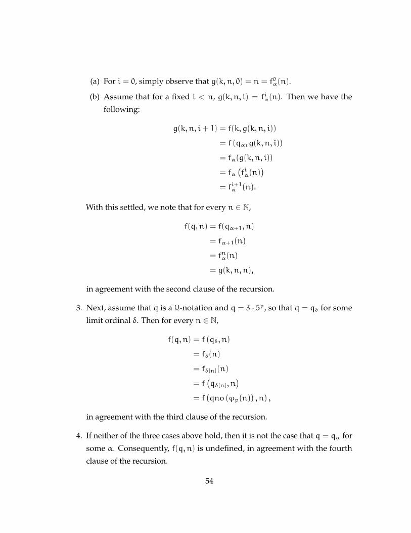
(a) For i = 0, simply observe that g(k, n, 0) = n = f0α(n).

(b) Assume that for a fixed i < n, g(k, n, i) = fiα(n). Then we have the

following:

g(k, n, i+ 1) = f(k, g(k, n, i))

= f (qα, g(k, n, i))

= fα(g(k, n, i))

= fα(fiα(n)

)= fi+1α (n).

With this settled, we note that for every n ∈ N,

f(q, n) = f(qα+1, n)

= fα+1(n)

= fnα(n)

= g(k, n, n),

in agreement with the second clause of the recursion.

3. Next, assume that q is a Q-notation and q = 3 · 5p, so that q = qδ for some

limit ordinal δ. Then for every n ∈ N,

f(q, n) = f (qδ, n)

= fδ(n)

= fδ[n](n)

= f(qδ[n], n

)= f (qno (ϕp(n)) , n) ,

in agreement with the third clause of the recursion.

4. If neither of the three cases above hold, then it is not the case that q = qα for

some α. Consequently, f(q, n) is undefined, in agreement with the fourth

clause of the recursion.

54

With this lemma established, we can at last demonstrate the infinite-time

effectiveness of our fast-growing hierarchy up to levelωCK1 .

Theorem 4.3.3. For every α < ωCK1 , fα is infinite-time computable.

As an immediate consequence of the preceding theorem, as well as Theorem

3.2.2 (our core result from Chapter 3), we can show that Σ∞ eventually dominates

a sizable portion of our fast-growing hierarchy.

Corollary 4.3.4. For every α < ωCK1 , Σ∞(n) >∗ fα(n).Proof of Theorem 4.3.3. It suffices to show that the functions f and g described in

the statement of Lemma 4.3.2 are infinite-time computable, as for a fixed α, we

would then have that fα = f(qα, ·) is infinite-time computable.

First, observe that the function g ′ : N4 → N given by the following primitive

recursion is evidently infinite-time computable via Theorems 2.1.1 and 2.1.3, as

well as the infinite-time computability of the relevant universal function:

g ′(e, k, n, 0) = n

g ′(e, k, n, i+ 1) = ϕ(N2,N)e (k, g ′(e, k, n, i)).

Moreover, the infinite-time computability of the function f ′ : N3 → N given

below follows directly from the partial infinite-time decidability of the predicate “o

is a Q-notation” (see Theorem 4.2.6), the infinite-time computability of the relevant

universal functions, and finally Theorems 2.1.1 and 2.1.3.

f ′(e, q, n) '

n+ 1 if q = 1

g ′(e, k, n, n) if q is a Q-notation and q = 2k

ϕ(N2,N)e (qno (ϕp(n)) , n) if q is a Q-notation and

q = 3 · 5p

undefined otherwise.

55

Lemma 2.1.2 assures the existence of an index e such that ϕ(N2,N)e = f ′(e, ·, ·).

Fixing such an e and taking f = ϕ(N2,N)e and g = g ′(e, ·, ·, ·) gives us infinite-time

computable functions that satisfy the recursion equations detailed in the statement

of Lemma 4.3.2, as a quick verification reveals.

The following theorem is in obvious analogy with Theorem 4.3.3.

Theorem 4.3.5. For every α < λ, fα is infinite-time eventually computable.

Proof. The argument is entirely analogous to that employed in proving Theorem

4.3.3: the statement and proof of Lemma 4.3.2 and Theorem 4.3.3 carry through

mutatis mutandis.

The preceding theorem and Theorem 3.2.2 show that Σe∞ eventually dominates

an even larger portion of our fast-growing hierarchy.

Corollary 4.3.6. For every α < λ, Σe∞(n) >∗ fα(n).

56

Chapter 5

Two Variants of Self-Modifying

Infinite-Time Turing Machines

In this chapter, we investigate self-modification for infinite-time Turing machines.

As a warm-up, we formulate, in Definition 5.1.1, a natural notion of Self-Modifying

Infinite-Time Turing Machine (SMITTM) which can modify its own instruction

list, and demonstrate that a natural family of these so-called “Class I SMITTMs” in

fact compute (and eventually compute) precisely the same functions as do ITTMs

(see Theorem 5.1.2).

In Section 5.2, we then define, via Definition 5.2.3, the collection of “Class ILT

SMITTMs,” which are not just capable of modifying their own instruction lists,

but can also (1) dynamically alter their limit convention, as well as (2) mount and

unmount new tapes mid-computation. In other words, Class ILT SMITTMs can

alter every aspect of their underlying hardware. Surprisingly, even this model of

infinitary computation admits an important and natural collection of machines

which compute (and eventually compute) precisely the same functions as the

original ITTM model (see Theorem 5.2.4). We finally devote Section 5.3 to the

development of the basic theory of the Class ILT model; among other things, we

formulate and prove analogues of the smn and universal theorems.

In a sense, this chapter is dual to Chapter 3: in that chapter, we placed a

57

resource restriction on our ITTMs (namely their number of states), and saw, via

Σ∞ and Σe∞, that even with such a restriction in place, the infinite-time computable

and eventually functions can still be quite “powerful” (in the sense of their growth

rates and infinite-time degree). This chapter, on the other hand, shows that adding

certain reasonable types of hardware to our ITTMs does not result in any additional

power.

5.1 Self-Modification of Instructions

We start by defining our first Self-Modifying Infinite-Time Turing Machine model.

Definition 5.1.1. Let n > 3, and fix a finite-time effective Godel numbering of

(n+ 1)-tape ITTM instructions. A Class I Self-Modifying Infinite-Time Turing

Machine (or Class I SMITTM)M consists of the following hardware (see Figure

5.1 on page 60 for an illustration):

• n data tapes (numbered 0 through n− 1), which are physically identical to

the tapes from the standard ITTM model. As with the standard model, two

tapes are predesignated to receive input and return output; for definiteness,

tapes 1 and 2 will handle input and output, respectively.

• A special instruction tape (numbered n), which, while also physically identi-

cal to the standard tapes, additionally subsumes the standard ITTM model’s

instructions and states. More precisely, a 1 on cell i of this tape indicates

the presence of the (n+ 1)-tape ITTM instruction with code i, while a 0 on

cell i denotes the absence thereof. (Informally, we could describe the former

situation by saying thatM has instruction i “loaded in its memory.”)

• A one-cell-wide head for reading and writing to both types of tapes simulta-

neously.

At the beginning of the computation, M is preloaded with a set of initial

commands on its instruction tape and receives input to its specially designated

data tape. In addition,M starts in state 0.

58

For successor stages of computation, M must account for the fact it may not

have exactly one relevant instruction loaded in its memory. (By a “relevant

instruction,” we mean one whose prefix matches the current state of M, as well as

what bits its tape head is currently reading.)

1. IfM has exactly one relevant instruction loaded, it simply executes that one.

2. On the other hand, if M has more than one relevant instruction loaded, it

“breaks the tie” by executing the one whose Godel number is smallest.

3. Finally, ifM has no relevant instructions loaded, it halts.

At limit stages,M behaves in a similar fashion to a standard ITTM:

1. Both the data type and instruction tape cells assume the lim sup of their

preceding values.

2. The tape head moves to the left-hand side of the tapes.

3. The current state will be changed to the LIMIT state.

♦

Note. Class I SMITTMs perform self-modification by writing a 0 or a 1 to their

instruction tapes; doing the former removes an instruction from memory, while

the latter loads one. 4

Remark. Notice how this model of computation is reminiscent of the Modified

Harvard computer architecture: while the data and instructions are located in

different portions of memory, both can be freely read and written to in tandem

(see [GCC04] for more details). 4

Let us first notice that there are surely functions which are Class-I-SMITTM-

computable but not ITTM computable: indeed, given any function f : N→ N, we

can “hard code” a lookup table for that function onto a Class I SMITTM instruction

tape.

The following theorem shows that if we restrict our attention to “reasonable”

instruction tapes, this state of affairs cannot occur.

59

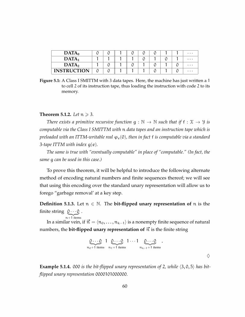
DATA0 0 0 1 0 0 0 1 1 · · ·DATA1 1 1 1 1 0 1 0 1 · · ·DATA2 1 0 1 0 1 0 1 0 · · ·

INSTRUCTION 0 0 1 1 1 0 1 0 · · ·

Figure 5.1: A Class I SMITTM with 3 data tapes. Here, the machine has just written a 1to cell 2 of its instruction tape, thus loading the instruction with code 2 to itsmemory.

Theorem 5.1.2. Let n > 3.

There exists a primitive recursive function g : N → N such that if f : X → Y is

computable via the Class I SMITTM with n data tapes and an instruction tape which is

preloaded with an ITTM-writable real ϕe(0), then in fact f is computable via a standard

3-tape ITTM with index g(e).

The same is true with “eventually computable” in place of “computable.” (In fact, the

same g can be used in this case.)

To prove this theorem, it will be helpful to introduce the following alternate

method of encoding natural numbers and finite sequences thereof; we will see

that using this encoding over the standard unary representation will allow us to

forego “garbage removal’ at a key step.

Definition 5.1.3. Let n ∈ N. The bit-flipped unary representation of n is the

finite string 0 · · · 0︸ ︷︷ ︸n+1 items

.

In a similar vein, if #»n = 〈n0, . . . , nk−1〉 is a nonempty finite sequence of natural

numbers, the bit-flipped unary representation of #»n is the finite string

0 · · · 0︸ ︷︷ ︸n0+1 items

1 0 · · · 0︸ ︷︷ ︸n1+1 items

1 · · · 1 0 · · · 0︸ ︷︷ ︸nk−1+1 items

.

♦

Example 5.1.4. 000 is the bit-flipped unary representation of 2, while 〈3, 0, 5〉 has bit-

flipped unary representation 0000101000000.

60

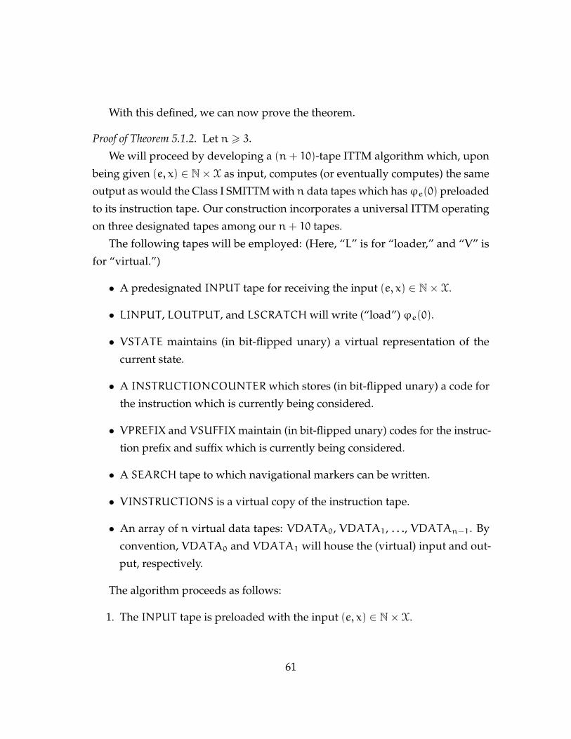
With this defined, we can now prove the theorem.

Proof of Theorem 5.1.2. Let n > 3.

We will proceed by developing a (n+ 10)-tape ITTM algorithm which, upon

being given (e, x) ∈ N× X as input, computes (or eventually computes) the same

output as would the Class I SMITTM with n data tapes which hasϕe(0) preloaded

to its instruction tape. Our construction incorporates a universal ITTM operating

on three designated tapes among our n+ 10 tapes.

The following tapes will be employed: (Here, “L” is for “loader,” and “V” is

for “virtual.”)

• A predesignated INPUT tape for receiving the input (e, x) ∈ N× X.

• LINPUT , LOUTPUT , and LSCRATCHwill write (“load”) ϕe(0).

• VSTATE maintains (in bit-flipped unary) a virtual representation of the

current state.

• A INSTRUCTIONCOUNTERwhich stores (in bit-flipped unary) a code for

the instruction which is currently being considered.

• VPREFIX and VSUFFIXmaintain (in bit-flipped unary) codes for the instruc-

tion prefix and suffix which is currently being considered.

• A SEARCH tape to which navigational markers can be written.

• VINSTRUCTIONS is a virtual copy of the instruction tape.

• An array of n virtual data tapes: VDATA0, VDATA1, . . ., VDATAn−1. By

convention, VDATA0 and VDATA1 will house the (virtual) input and out-

put, respectively.

The algorithm proceeds as follows:

1. The INPUT tape is preloaded with the input (e, x) ∈ N× X.

61

2. In ω many steps, we fill our VSTATE, VPREFIX, VSUFFIX, SEARCH, and

INSTRUCTIONCOUNTER tapes with 1s.

3. We now copy e and x to LINPUT and the VDATA0 tape, respectively.

4. The L tapes use a universal ITTM to computeϕe(0). If and when this compu-

tation is finished, we copy the contents of LOUTPUT to VINSTRUCTIONS.

5. Write out a bit-flipped unary representation for the initial VSTATE.

6. For the remainder of the run-time, we repeatedly simulate a single Class I

SMITTM step using a finite number of ITTM steps:

(a) In finitely many steps, set the INSTRUCTIONCOUNTER’s contents to

0 (in bit-flipped unary). For convenience, we let n be the contents of the

INSTRUCTIONCOUNTER.

(b) In finite time, decode n and write out bit-flipped unary representations

of its prefix and suffix to VPREFIX and VSUFFIX, respectively.

(c) Check (in finitely many steps) if instruction n is loaded (by consulting

the VINSTRUCTIONS tape) and if the current prefix bits and VSTATE

match the corresponding contents of VPREFIX.

i. If so, we...

A. write the bits indicated by the VSUFFIX to the VDATAi tapes

and VINSTRUCTIONS tape,

B. clear and then update the VSTATE (halting if necessary),

C. mark the new location for the tape head on the SEARCH tape

with a 0marker,

D. clear the VPREFIX and VSUFFIX,

E. move the tape head to the 0marker on the SEARCH tape and

replace it with a 1, and

F. go to step 6a.

ii. Otherwise, we...

62

A. clear the VPREFIX and VSUFFIX,

B. increment n, and

C. return to step 6b.

7. At limit stages, there is no need for garbage removal, as VSTATE, VPREFIX,

VSUFFIX, INSTRUCTIONCOUNTER, and SEARCH will always contain an

all-1s configuration, except for when we failed to find a relevant instruction

to execute in a previous successor step; in this case, there will be a telltale 0

on the INSTRUCTIONCOUNTER. If we detect this, we simply halt.

By Theorem 2.2.1 (respectively, Theorem 2.2.2), there exists a 3-tape ITTM

computable (respectively, eventually computable) function f : N× X→ Y which

carries out the algorithm above. We can then obtain the desired primitive recursive

g : N→ N by applying the smn Theorem to f. (Note that the smn Theorem yields the

same function g for both computable and eventually computable functions.)

Note. If we were so inclined, we could use the preceding theorem to formulate

an effective enumeration of “reasonable” Class-I-SMITTM-computable functions,

and then from there develop the corresponding smn and universal theorems, as

well as other crucial aspects of the basic theory. However, the arguments would

be entirely analogous to those we will perform for the corresponding results for

Class ILT SMITTMs in Section 5.3. 4

5.2 Passing from Class I to Class ILT SMITTMs

Our next order of business will be define the Class ILT SMITTMs, which will

be able to dynamically modify (1) their instruction list, (2) the underlying limit

convention, and (3) which tapes are mounted and unmounted.

To this end, we will first need to give a precise formulation for the instructions

such machines will process.

Definition 5.2.1. Anω-tape instruction for ITTMs consists of a finite prefix and

suffix. The prefix contains exactly one of each of the following types of strings:

63

• A finite sequence of symbols of the form IbDi0ai0Di1ai1 · · ·Dik−1aik−1 , where

i0, i2, . . ., ik−1 is a finite increasing sequence of natural numbers, b ∈ {0, 1},

and aim ∈ {0, 1} for every 0 6 m 6 k− 1.

• Exactly one of the following two types of substrings:

– Si, where i ∈ N.

– LIMIT .

On the other hand, the suffix contains exactly one of each of the following

types of strings:

• A finite sequence of symbols of the form IbDi0ai0Di1ai1 · · ·Dik−1aik−1 , where

i0, i2, . . ., ik−1 is a finite increasing sequence of natural numbers, b ∈ {0, 1},

and aim ∈ {0, 1} for every 0 6 m 6 k− 1.

• Exactly one of the substrings LS or LI.

• A substring UNMOUNTi MOUNTj, where i, j > 2.

(Note that for the sake of uniformity in our notation, we DO allow i = j; an

instruction with this kind of substring in its prefix effectively mounts and

unmounts no tapes. In addition, note that we have explicitly disallowed

the values 0 and 1 for i and j. this is to prevent unmounting the input and

output tapes.)

• Exactly one of the substrings L or R.

• Exactly one of the following two types of substrings:

– Si, where i ∈ N.

– HALT .

♦

Example 5.2.2. The following are two examples of validω-tape ITTM instructions:

64

1. I1 D10 D21 S3 → I0 D31 D50 LS UNMOUNT10 MOUNT5 L HALT . This

instruction should be interpreted as follows:

“If we are...

(a) reading a 1 on the instruction tape,

(b) reading a 0 and 1 on data tapes 1 and 2 (respectively), and

(c) currently in state 3,

then...

(a) write a 0 to the instruction tape,

(b) write a 1 and 0 on data tapes 3 and 5 respectively,

(c) switch to the lim sup convention,

(d) unmount data tape 10,

(e) mount data tape 5,

(f) move the tape head to the left, and

(g) halt the computation.”

2. I1 D10 D21 D41 LIMIT → I1 D31 D50 LI UNMOUNT2 MOUNT2 R S9,

which is interpreted thusly:

“If we are...

(a) reading a 1 on the instruction tape,

(b) reading a 0, 1, and 1 on data tapes 1, 2, and 4 (respectively), and

(c) currently in the LIMIT state,

then...

(a) write a 1 to the instruction tape,

(b) write a 1 and 0 on data tapes 3 and 5 respectively,

(c) switch to the lim inf convention,

65

(d) move the tape head to the right, and

(e) transition to state 9.”

(Note that no tape is mounted nor unmounted.)

We can now formally define the Class ILT SMITTMs.

Definition 5.2.3. Fix a finite-time effective Godel numbering ofω-tape instructions

for ITTMs. A Class ILT Self-Modifying Infinite-Time Turing Machine (or Class

ILT SMITTM)M consists of the following hardware (see Figure 5.2 on 68 for an

illustration):

• Countably many data tapes, which are physically identical to the tapes

from the standard ITTM model, and canonically labeled asDATA0,DATA1,

DATA2, . . .. As with the standard model, two tapes are predesignated to

receive input and return output; for uniformity in notation, these will be

DATA0 and DATA1, respectively.

• A special instruction tape, which functions similarly to the instruction tape

of a Class I SMITTM. More precisely, a 1 on cell i of this tape indicates the

presence of the ω-tape ITTM instruction with code i, while a 0 on cell i

denotes the absence thereof.

• A one-cell-wide head for reading and writing to both types of tapes simulta-

neously. The tape head will only be able to read and write from tapes which

are currently mounted.

At the beginning of the computation, M is preloaded with a set of initial

commands on its instruction tape, and only three data tapes (DATA0, DATA1,

and DATA2) are initially mounted. In addition, the initial input is passed to the

input tape ofM, andM starts in state 0.

For successor stages of computation, M acts like a Class I ITTM, save that

any instruction which references an unmounted tape in its prefix and/or suffix is

deemed irrelevant:

66

1. IfM has exactly one relevant instruction loaded, it simply executes that one.

2. On the other hand, if M has more than one relevant instruction loaded, it

“breaks the tie” by executing the one whose Godel number is smallest.

3. Finally, ifM has no relevant instructions loaded, it halts.

At limit stages,M behaves as follows:

1. The data and instruction tape cells are updated in one of two possible ways:

(a) If the suffix substring LS occurred unboundedly often in the instructions

which have been executed thus far, the tape cells assume the lim sup of

their preceding values.

(b) Otherwise, the tape cells assume the lim inf of their preceding values.

2. Any tapes which have been mounted unboundedly often stay mounted; all

other tapes are unmounted.

3. The tape head moves to the left-hand side of the tapes.

4. The current state is changed to the LIMIT state.

♦

We can now prove the analogue of Theorem 5.1.2 for Class ILT SMITTMs.

Theorem 5.2.4. Let n ∈ N.

There exists a primitive recursive function g : N → N such that if f : X → Y is

computable via the Class ILT SMITTM with an instruction tape which is preloaded with

an ITTM-writable real ϕe(0), then in fact f is computable via a standard 3-tape ITTM

with index g(e).

The same is true with “eventually computable” in place of “computable.” (In fact, the

same choice of g can be used in this case.)

67

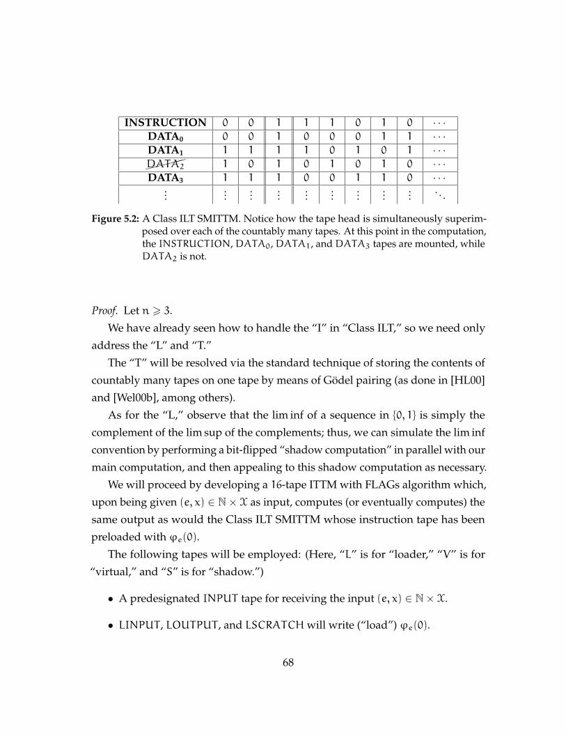
INSTRUCTION 0 0 1 1 1 0 1 0 · · ·DATA0 0 0 1 0 0 0 1 1 · · ·DATA1 1 1 1 1 0 1 0 1 · · ·�����DATA2 1 0 1 0 1 0 1 0 · · ·DATA3 1 1 1 0 0 1 1 0 · · ·

......

......

......

......

... . . .

Figure 5.2: A Class ILT SMITTM. Notice how the tape head is simultaneously superim-posed over each of the countably many tapes. At this point in the computation,the INSTRUCTION, DATA0, DATA1, and DATA3 tapes are mounted, whileDATA2 is not.

Proof. Let n > 3.

We have already seen how to handle the “I” in “Class ILT,” so we need only

address the “L” and “T.”

The “T” will be resolved via the standard technique of storing the contents of

countably many tapes on one tape by means of Godel pairing (as done in [HL00]

and [Wel00b], among others).

As for the “L,” observe that the lim inf of a sequence in {0, 1} is simply the

complement of the lim sup of the complements; thus, we can simulate the lim inf

convention by performing a bit-flipped “shadow computation” in parallel with our

main computation, and then appealing to this shadow computation as necessary.

We will proceed by developing a 16-tape ITTM with FLAGs algorithm which,

upon being given (e, x) ∈ N× X as input, computes (or eventually computes) the

same output as would the Class ILT SMITTM whose instruction tape has been

preloaded with ϕe(0).

The following tapes will be employed: (Here, “L” is for “loader,” “V” is for

“virtual,” and “S” is for “shadow.”)

• A predesignated INPUT tape for receiving the input (e, x) ∈ N× X.

• LINPUT , LOUTPUT , and LSCRATCHwill write (“load”) ϕe(0).

68

• VSTATE maintains (in bit-flipped unary) a virtual representation of the

current state.

• A INSTRUCTIONCOUNTERwhich stores (in bit-flipped unary) a code for

the instruction which is currently being considered.

• VPREFIX and VSUFFIXmaintain (in bit-flipped unary) codes for the instruc-

tion prefix and suffix which is currently being considered.

• A SEARCH tape to which navigational markers can be written.

• VINSTRUCTIONS contains a virtual copy of the instruction tape.

• S-VINSTRUCTIONS contains a bit-flipped copy of the VINSTRUCTIONS

tape.

• MOUNTSTATUS keeps track of which tapes are mounted and unmounted.

For example, a 1 in cell 4 would indicate that tape 4 is mounted.

• A VOUTPUT tape which will be used to store a virtual copy of the DATA1tape, and which will also serve as the predesignated tape for output.

• An S-VOUTPUT tape which stores a bit-flipped copy of the VOUTPUT tape.

• A VDATA tape which, via a Godel pairing, stores virtual copies of every

DATAi tape (for all i 6= 1).

• An S-VDATA tape which stores a bit-flipped copy of the VDATA tape.

In addition, we will use a LIMSUP flag to keep track of which limit convention

is currently in play.

The algorithm proceeds as follows:

1. The INPUT tape is preloaded with the input (e, x) ∈ N× X.

2. In ω many steps, we fill our VSTATE, VPREFIX, VSUFFIX, SEARCH, and

INSTRUCTIONCOUNTER tapes with 1s, and write 1s to cells 0, 1, and 2 of

ourMOUNTSTATUS tape.

69

3. We now copy e and x to LINPUT and the 0th slice of the VDATA tape,

respectively.

4. The L tapes use a universal ITTM to computeϕe(0). If and when this compu-

tation is finished, we copy the contents of LOUTPUT to VINSTRUCTIONS.

5. Write out a bit-flipped unary representation for the initial VSTATE.

6. For the remainder of the run-time, we repeatedly simulate a single Class ILT

SMITTM step using a finite number of ITTM steps:

(a) In finitely many steps, set the INSTRUCTIONCOUNTER’s contents to

0 (in bit-flipped unary). For convenience, we let n be the contents of the

INSTRUCTIONCOUNTER.

(b) In finite time, decode n and write out bit-flipped unary representations

of its prefix and suffix to VPREFIX and VSUFFIX, respectively.

(c) Check (in finitely many steps) if instruction n is loaded (by consulting

the VINSTRUCTIONS tape) and if the current prefix bits and VSTATE

match the corresponding contents of VPREFIX.

i. If so, we...

A. write the bits dictated by the VSUFFIX to the VINSTRUCTION

and VOUTPUT tapes, as well as the appropriate slices of the

VDATA tape; we simultaneously write their complements to

the corresponding shadow tapes.

B. clear and then update the VSTATE (halting if necessary),

C. turn the LIMSUP flag ON or OFF (as according to whether or

not a code for LS appears in the VSUFFIX),

D. write to the appropriate portions of theMOUNTSTATUS tape,

E. mark the new location for the tape head on the SEARCH tape

with a 0marker,

F. clear the VPREFIX and VSUFFIX,

70

G. move the tape head to the 0marker on the SEARCH tape and

replace it with a 1, and

H. go to step 6a.

ii. Otherwise, we...

A. clear the VPREFIX and VSUFFIX,

B. increment n,

C. and return to step 6b.

7. At limit stages, there is no need for garbage removal, as VSTATE, VPREFIX,

VSUFFIX, INSTRUCTIONCOUNTER, and SEARCH will always contain an

all-1s configuration, except for when we failed to find a relevant instruction

to execute in a previous successor step: in this case, there will be a telltale 0

on the INSTRUCTIONCOUNTER. If we detect this, we immediately halt.

That said, we still need to carry out the prescribed limit convention:

(a) If the LIMSUP flag is ON, we shall copy, in ω many steps, the bit-

flipped contents of the VINSTRUCTIONS, VOUTPUT , and VDATA

tapes to the corresponding shadow tapes.

(b) On the other hand, if the LIMSUP flag is OFF, we instead copy, in

ω many steps, the bit-flipped contents of the S-VINSTRUCTIONS,

S-VOUTPUT , and S-VDATA tapes to the corresponding virtual tapes.

(Thus taking the lim inf.)

By Theorems 2.2.1 (respectively, Theorem 2.2.2), there exists a 3-tape ITTM

computable (respectively, eventually computable) function f : N× X→ Y which

carries out the algorithm above. We can then obtain the desired primitive recursive

g : N→ N by applying the smn Theorem to f. (Note that the smn Theorem yields the

same function g for both computable and eventually computable functions.)

We now “work backwards” to obtain the following theorem.

71

Theorem 5.2.5. There exists a primitive recursive h : N→ N such that for every n ∈ N,

the partial functions ϕ(X,Y)n and ϕe,(X,Y)n can be computed via the Class ILT SMITTM

with an instruction tape which has been preloaded with ϕh(n)(0) on its instruction tape.

Proof. To avoid getting caught up in minutia about how our instructions are coded,

we will describe a finite-time algorithm for obtaining a total computable h(n)

from n, and then sketch why h is in fact primitive recursive.

Given an index n for a 3-tape ITTM program, we can decode n in finitely many

steps and obtain codes a0, a1, . . ., ak−1 for its instructions. We can then uniformly

convert these codes to codes b0, b1, . . ., bk−1 for the instructions for an ω-tape

ITTM program which (1) act on data tapes 0-2 exactly as instructions a0, a1, . . .,

ak−1 do to tapes 0-2 of ITTM program n and (2) completely ignore the remaining

data tapes.

We next sort these new codes in ascending order, say c0, c1, . . ., ck−1, and

then uniformly obtain an index n ′ for a 3-tape ITTM program with n non-halting,

non-limit states, which, while ignoring the contents of the INPUT and SCRATCH

tapes, moves the tape head to cell array c0 and writes a 1 to the OUTPUT tape,

moves the tape head to cell array c1 and writes another 1 to theOUTPUT tape, . . .,

moves the tape head to cell array ck−1 and writes one last 1 to the OUTPUT tape,

and then HALTs.

By construction, the Class ILT SMITTM withϕn ′(0) preloaded to its instruction

tape will compute ϕ(X,Y)n and eventually compute ϕe,(X,Y)n , and the uniformity

and effectiveness of our procedure above ensure, by the Church-Turing Thesis,

that h(n) := n ′ is a finite-time total computable function.

To see that h is primitive recursive, note first that the passage from a0, a1,

. . ., ak−1 to b0, b1, . . ., bk−1, as well as that from b0, b1, . . ., bk−1 to c0, c1, . . .,

ck−1, is primitive recursive in character: in the case of the former, we are merely

“converting” codes for ITTM instructions to their analogousω-tape instructions,

and as for the latter, sorting a finite list of integers is evidently a primitive recursive

operation. Finally, assembling the index n ′ from the codes c0, c1, . . ., ck−1 is a

primitive recursive operation, as n ′ is obtained by concatenating all of the relevant

72

instructions into a program, and such concatenation is well-known to be primitive

recursive.

5.3 Developing the Theory for Class ILT SMITTMs

We now finish the chapter by formulating, for Class ILT SMITTM computations,

natural analogues for the classical results of both finite- and infinite-time Turing

machine computations.

Theorem 5.2.4 implicitly gives us an effective enumeration of “reasonable”

Class ILT SMITTMs, which we now state formally.

Definition 5.3.1. Fix a primitive recursive g : N→ N as guaranteed by Theorem

5.2.4. For every n ∈ N and pair of product spaces X, Y, we set

ψ(X,Y)n = ϕ

(X,Y)g(n) and ψe,(X,Y)n = ϕ

e,(X,Y)g(n) .

♦

Note. In this notation, Theorem 5.2.5 can be restated more concisely:

There exists a primitive recursive h : N → N such that for every

n ∈ N and pair of product spaces X, Y,

ϕ(X,Y)n = ψ

(X,Y)h(n) and ϕe,(X,Y)n = ψ

e,(X,Y)h(n) .

4

Now that we have an effective means of switching between ϕ-codes and

ψ-codes, we can establish an smn Theorem.

Theorem 5.3.2 (smn Theorem for Class ILT SMITTMs). Let X be a type 0 product

space.

Then there exists a primitive recursive s : N × X → N such that for every #»n ∈ X,

y ∈ Y, and p ∈ N,

ψ(X×Y,Z)p ( #»n, y) ' ψ(Y,Z)

s(p, #»n)(y) and ψe,(X×Y,Z)p ( #»n, y) ' ψe,(Y,Z)

s(p, #»n) (y).

73

Proof. Fix a primitive recursive function h : N → N as guaranteed by Theorem

5.2.5. For an arbitrary #»n ∈ X, y ∈ Y, and p ∈ N,

ψ(X×Y,Z)p ( #»n, y) ' ϕ(X×Y,Z)

g(p) ( #»n, y)

' ϕ(Y,Z)s ′(g(p), #»n)(y)

' ψ(Y,Z)h(s ′(g(p), #»n))(y),

(In the third step, we obtain the primitive recursive function s ′ : N×N→ N by

invoking the smn theorem for ITTM-computable functions.)

Note further that by the smn theorem for ITTM-eventually computable functions,

the above sequence of equalities holds with ψe and ϕe in place of ψ and ϕ

(respectively), and via the same choice of s ′.

Thus, the primitive recursive function s : N × X → N given by s(p, #»n) :=

h (s ′(g(p), #»n)) is as we desire.

A similar style of argument works just as well for demonstrating the existence

of the relevant universal machines.

Theorem 5.3.3 (Universal Machines for Class ILT SMITTMs). Let X,Y be product

spaces. Then the maps ψU,(X,Y) : N × X → Y and ψU,e,(X,Y) : N × X → Y which are

respectively given by

ψU,(X,Y)(n, x) ' ψ(X,Y)n (x) and ψU,e,(X,Y)(n, x) ' ψe,(X,Y)n (x)

are Class-ILT-SMITTM-computable and Class-ILT-SMITTM-eventually computable,

respectively.

Proof. Fix a primitive recursive function g : N → N as guaranteed by Theorem

5.2.4.

For an arbitrary n ∈ N, x ∈ X, and y ∈ Y,

ψU,(X,Y)(n, x) ' ψ(X,Y)n (x)

' ϕ(X,Y)g(n) (x)

' ϕU,(X,Y)(g(n), x).

74

Now, simply observe that the final step is ITTM-computable (by the Universal

Machine Theorem for ITTM-computable functions), and hence Class-ILT-SMITTM-

computable (by Theorem 5.2.5).

A similar argument employing the Universal Machine Theorem for eventu-

ally computable ITTM functions establishes that ψU,e,(X,Y) is Class-ILT-SMITTM-

eventually computable.

We now classify the ordinals which are writable (or eventually writable) by

“reasonable” Class ILT SMITTMs. We first observe that, like their ITTM counter-

parts, such writable (or eventually writable) ordinals are closed downward:

Theorem 5.3.4 (No Gaps Theorem for Class ILT SMITTMs). If α < β and β is

writable (or eventually writable) via a Class ILT SMITTM with initial instruction tape an

ITTM-writable real, then so is α.

Proof. If a code for β, say x ∈ 2N, is writable by such a Class ILT SMITTM, then

by Theorem 5.2.4, there in fact exists an ITTM program with index p such that

ϕp(0) = x.

Let n ′ ∈ N be such that ≺x �n ′ has order type α. Then Theorem 2.1.1 yields an

ITTM-computable function f : N→ 2N which is given by f(n) := rest (ϕp(0), n ′).

Observe that f produces, from the trivial input n = 0, a code for α. By Theorem

5.2.5, f is computable via a Class ILT SMITTM whose instruction tape has been

preloaded with an ITTM-writable real. Thus, α enjoys the same writability as β.

A similar argument works just as well with β eventually writable: one simply

constructs f by instead composing rest with an ITTM-eventually computable

function which eventually writes a code for β.

With this result “in our quiver,” we can complete the our classification by

determining the relevant sumprema.

Theorem 5.3.5. λ (respectively, ζ) is the supremum of the ordinals which are writable

(respectively, eventually writable) by a Class ILT SMITTM whose instruction tape has

been preloaded with an ITTM-writable real.

75

Proof. We will restrict our attention to the case of writable ordinals, as the argu-

ment for the eventual writable ordinals carries through mutatis mutandis.

Clearly, the desired supremum can be no greater than λ, as if we could write λ

using an appropriate Class ILT SMITTM, then by Theorem 5.2.4, we could in fact

write λwith an ITTM, which is known to be impossible (see [HL00]).

On the other hand, the supremum is at least λ, as by Theorem 5.2.5, every

ITTM-writable ordinal is writable by a Class ILT SMITTM with ITTM-writable

instruction tape.

Thus, the supremum must be exactly equal to λ.

Let us now observe that the Class ILT SMITTMs can be relativized to both

oracles z ∈ 2N and A ⊆ 2N in the obvious way. To finish off this chapter, we

showcase the natural relativizations of Theorems 5.2.4 and 5.2.5.

Theorem 5.3.6. Let z ∈ 2N and A ⊆ 2N.

There exists a primitive recursive function g : N → N such that, for every z ∈ 2N

(respectively, A ⊆ 2N), if f : X → Y is computable via the Class ILT SMITTM with an

instruction tape which is preloaded with an ITTM-writable real ϕe(0) and an oracle z

(respectively, A), then in fact f is computable via a standard 3-tape ITTM with index g(e)

and an oracle z (respectively, A).

The same is true with “eventually computable” in place of “computable.” (In fact, the

same choice of g can be used in this case.)

Proof. The algorithm we outlined in the proof of Theorem 5.2.4 almost carries

through completely, save that we also need to maintain a shadow tape for the

ORACLE. In step 6c, we also need (in finite time) to read a bit from the ORACLE

tape, and for oracles A ⊆ 2N, we additionally need to assess if the current real on

the ORACLE lies in A and write a bit to the ORACLE tape. Now apply Theorem

2.3.3.

Theorem 5.3.7. Let z ∈ 2N and A ⊆ 2N.

There exists a primitive recursive h : N → N such that for every e ∈ N and z ∈ 2N

(respectively, A ⊆ 2N), the partial function ϕze : X→ Y (respectively, ϕAe : X→ Y) can

76

be z-computed (respectively A-computed) via the Class ILT SMITTM with an instruction

tape which has been preloaded with ϕh(e)(0).

Proof. The same algorithm that we employed in proving Theorem 5.2.5 works

here, save that we now deal with codes of appropriate oracle instructions.

77

Chapter 6

Conclusions and Future Work

6.1 Conclusions and Future Work Based on Chapter 3

In Chapter 3, we formulated analogues of Rado’s Σ busy beaver function for

the setting of infinite-time computability and eventual computability, namely Σ∞and Σe∞ (respectively), and showed that both possess the same natural eventual

domination property as Σ. Moreover, we also showed that Σ∞ eventually dom-

inates all sD-recursive functions f : N → N, and as a consequence thereof, all

Π11-recursive functions f : N→ N, as well asWeakRayo. Lastly, we showed that

the infinite-time degree of Graph (Σ∞) was 0O, and that that of Graph (Σe∞) was

either (1) equal to 0Oζ or (2) not accidentally writable.

Based on these results, it would be interesting to determine precisely which

Σ-pointclasses Γ are such that Σ∞ eventually dominates all Γ -recursive functions

f : N→ N. In a similar vein, we might consider defining analogues of WeakRayo

for certain fragments of second-order arithmetic, and then considering which such

analogues are eventually dominated by Σ∞.

One more natural direction for future work would be to completely settle the

infinite-time degree of Graph (Σe∞), as either of the two possibilities we specified

are extremely interesting: because [Kle07] showed that 0Oζ ≡∞ s, where s denotes

the so-called “lightface infinite-time stabilization program,” one would suspect

78

that Graph (Σe∞) ≡∞ 0Oζ , in analogy with our result that Graph (Σ∞) ≡∞ 0O. As

such, if the infinite-time degree of Graph (Σe∞) were not accidentally writable, so

that Graph (Σe∞) 6≡∞ 0Oζ , we would have a curious deviation from the typical

parallel between halting and stabilizing infinite-time computations.

6.2 Conclusions and Future Work Based on Chapter 4

In Chapter 4, we constructed a fast-growing hierarchy 〈fα α < ζ〉, and arranged

things in such a way that fα is infinite-time computable (respectively, eventually

computable) for all α < ωCK1 (respectively, α < λ); consequently, Σ∞ (respectively,

Σe∞) eventually dominates all the fα for α < ωCK1 (respectively, α < λ).

As the relations <O, <O+ , and <O++ are rooted trees of height ωCK1 , λ, and

ζ, respectively, it would be ideal if we could obtain a more “naturally effective”

version of our fast-growing hierarchy. More precisely, we would like to have fαbe finite-time computable, infinite-time computable, and infinite-time eventually

computable for α < ωCK1 , α < λ, and α < ζ, respectively. The corresponding

eventual domination results for Σ, Σ∞, and Σe∞ would surely make for a nice

parallel.

One further way that we could refine our fast-growing hierarchy would be

to find some “effective majorization” thereof: not only do we want each fα to be

appropriately computable, but we would also like to have, for all α < β < ζ, that

fβ(n) >∗ fα(n). Indeed, as Schmidt details in [Sch77], most previously defined

fast-growing hierarchies have this majorization property. Moreover, this property

would make the associated eventual domination results for Σ, Σ∞, and Σe∞ all the

more impressive.

(It is also worth noting that in [Kle07], Klev showed that O, O+, and O++ are

“computably isomorphic” to the finite-time halting problem, the lightface infinite-

time halting problem, and the lightface infinite-time stabilization problem. As

such, there is a clear parallel between the future work we have proposed in this

section with that of the previous one.)

79

6.3 Conclusions and Future Work Based on Chapter 5

In Chapter 5, we devised two variants of Self-Modifying Infinite-time Turing

Machines (SMITTMs), and showed that, provided one restricts their attention to

those SMITTMs whose instruction tapes have been preloaded with an infinite-

time writable real, the SMITTMs and ITTMs compute (and eventually compute)

precisely the same functions; we also cultivated the basic theory thereof.

Recall that in the setting of classical computability, it is generally believed that

all reasonable models of finite-time computation will compute precisely the same

functions. On the other hand, as outlined in [DHK07], there are many incom-

parable models of infinite-time computation, and thus, one naturally wonders

which model is “best.” Our work here shows that the original ITTM model is

highly robust, and as such, suggests that it might furnish the “right” model of

infinite-time computation.

To test this claim, it would be natural to figure out ways to add self-modification

to other models of infinite-time computation, and then determine if their under-

lying computational power is preserved or compromised. In particular, carrying

out this study for Koepke’s Ordinal Turing Machines (OTMs) would, depending

on the outcome, affirm or dispute Carl’s claim in [Car13] that the OTM model is

in fact “right.”

Alternatively, we could consider ways to enhance the SMITTM models in yet

more “effectiveness-preserving” ways. More specifically, it would be easier to

design SMITTM programs if we could formulate an “SMITTM with ROM”; i.e., an

SMITTM which has two separate instruction lists, one of which can be modified

in a similar fashion as for the Class I and Class ILT models, and the other of which

would be “read-only.” (In a sense, such an SMITTM would have an immutable

“operating system.”)

80

6.4 Another Avenue for Future Work

As we mentioned in Chapter 1, the µ operator is naturally thought of as being an

“unbounded search operator”: indeed, if a function g : N× X→ Y is finite-time

computable, the natural algorithm for computing µn (g(n, x) = 0) would involve

systematically attempting to compute g(0, x), g(1, x), g(2, x), . . . until and unless

a witness n ∈ N is found such that g(n, x) = 0.

In the setting of infinite-time computability, however, “unbounded” is some-

thing of a misnomer: if a function g : N × X → Y is infinite-time computable,

we can undertake the same systemic computations g(0, x), g(1, x), g(2, x), . . . as

before, and, by flashing a special flag “on” and “off” whenever we transition to a

new such computation, we can recognize, at limit stages, if we have computed

g(n, x) for all n ∈ N. Under this condition, we can return a special output config-

uration (such as 1111 · · · ) to indicate that we computed g(n, x) for all n ∈ N and

failed to find a witness n ∈ N such that g(n, x) = 0.

The preceding suggests that we should consider a “smart” µ operator which

returns either (1) the witness n ∈ N (if one exists) or (2) a special output if g(n, x)

was defined for all n ∈ N, yet no witness was found; on the other hand, if g(n, x)

is undefined for some n ∈ N, the operator is undefined.

The infinite-time algorithm we sketched above shows that the infinite-time

computable functions are closed under this operator. It would be extremely useful

to have the analogous result for the infinite-time eventually computable functions

as well. Without going into details, a “smart” µ operator would establish that

the Q- and Q+-notations from Chapter 4 are in fact infinite-time decidable and

eventually infinite-time decidable, respectively.

(It is also worth noting that Chapters 3 and 5 hint at the need for a “smart” µ

operator as well: there is a straightforward proof that Σ∞(n) >∗ WeakRayo (n)using a “smart” unbounded search through all the formulas of first-order arith-

metic with one free variable, and our ITTM simulations of the Class I and ILT

SMITTMs conducts a kind of “smart” unbounded search when trying to determine

if there are any relevant instructions loaded.)

81

Index

2N, 3

accidentally writable

ordinal, 10

real, 10

BB-n, 33

BB∞-n, 33

BBe∞-n, 33

bit-flipped unary representation

of a finite sequence of natural num-

bers, 60

of a natural number, 60

blank tape, 10

Cantor space, 3

>∗, 5

eventually writable

ordinal, 10

real, 10

fast-growing hierarchy, 45

ft-ϕp, 9

function

infinite-time computable, 8

infinite-time eventually computable,

8

partial, 4

total, 4

fundamental sequence, 44

Γ -recursive function, 37

halting computation, 8

A ≡∞ B, 11

infinite-time decidable, 8

infinite-time degree, 11

accidentally writable, 41

eventually writable, 41

infinite-time eventually decidable, 8

infinite-time eventually semi-decidable,

8

infinite-time reducible, 11

infinite-time semi-decidable, 8

A 6∞ B, 11

A <∞ B, 11

ITTM

instruction

prefix, 6

suffix, 6

82

standard, 6

with FLAGS, 26

Kleene’s O, 45

analogue in F, 46

λ, 10

µ operator, 5

O, 45

OF, 46

OF-notation, 46

O+, 46

O++, 46

|n|OF , 46

|q|O, 48

|q|O+ , 48

|q|O++ , 48

ω-tape instruction for ITTMs, 63

ωCK1 , 10

<O, 45

<OF , 46

partially decidable, 9

ϕ(X,Y)p , 9

ϕp, 9

ϕe,(X,Y)p , 9

ϕep, 9

pointclass, 3

≺x, 4

primitive recursion, 5

primitive recursive, 6

product space

pairing of points, 4

products of, 3

type 0, 3

type 1, 3

ψ(X,Y)n , 73

ψe,(X,Y)n , 73

Q-notation, 48

Q+-notation, 48

Q++-notation, 48

qno, 49

qno+, 49

qno++, 50

Rayo (n), 39

real numbers, 3

reals, 3

rest, 4

sD, 38

Σ (function), 33

Σ (ordinal), 10

Σ∞, 34

Σe∞, 34

Σ-pointclass, 37

SMITTM

Class I, 58

Class ILT, 66

stabilizing computation, 8

states (p), 33

substitution, 5

83

unbounded minimization, 5

weak jump for z, 11

zO, 11

WeakRayo (n), 39

writable

ordinal, 10

real, 10

ζ, 10

84

Bibliography

[Car13] Merlin Carl, Towards a Church-Turing-thesis for infinitary computations,

arXiv preprint arXiv:1307.6599 (2013).

[CH13] Samuel Coskey and Joel David Hamkins, Infinite time Turing machines

and an application to the hierarchy of equivalence relations on the reals, Book

chapter, ASL Lecture Notes in Logic NL volume Effective Mathematics

of the Uncountable 41 (2013).

[DHK07] Ioanna Dimitriou, Joel David Hamkins, and Peter Koepke,

BIWOC–Bonn international workshop on ordinal computability, Bonn Logic

Reports (2007).

[GCC04] James H Grosbach, Joshua M Conner, and Michael Catherwood,

Modified Harvard architecture processor having program memory space

mapped to data memory space, April 27 2004, US Patent 6,728,856.

[Grz53] Andrzej Grzegorczyk, Some classes of recursive functions, Rozprawy

Matematyczne 4 (1953), 1–45.

[Her08] Joachim Hertel, Computing the uncomputable Rado sigma function,

Mathematica Journal 11 (2008), no. 2, 270.

[HL00] Joel David Hamkins and Andrew Lewis, Infinite time Turing machines,

The Journal of Symbolic Logic 65 (2000), no. 02, 567–604.

[HL02] , Post’s problem for supertasks has both positive and negative solutions,

Archive for Mathematical Logic 41 (2002), no. 6, 507–523.

85

[HS01] Joel David Hamkins and Daniel Evan Seabold, Infinite time Turing

machines with only one tape, Mathematical Logic Quarterly 47 (2001),

no. 2, 271–287.

[Kle07] Ansten Mørch Klev, Extending Kleene’s O using infinite time Turing

machines, or how with time she grew taller and fatter, Master’s thesis,

Universiteit van Amsterdam, 2007.

[Kle09] , Infinite time extensions of Kleene’s O, Archive for Mathematical

Logic 48 (2009), no. 7, 691–703.

[LW70] Martin H Lob and Stanley S Wainer, Hierarchies of number-theoretic

functions. I, Archive for Mathematical Logic 13 (1970), no. 1, 39–51.

[Mos09] Yiannis N Moschovakis, Descriptive set theory, no. 155, American

Mathematical Society, 2009.

[Rad62] Tibor Rado, On non-computable functions, Bell System Technical Journal

41 (1962), no. 3, 877–884.

[Ray] Augustın Rayo, Big number duel,

http://web.mit.edu/arayo/www/bignums.html, Accessed:

04-01-2015.

[Rog67] Hartley Rogers, Theory of recursive functions and effective computability,

vol. 126, McGraw-Hill New York, 1967.

[Sch77] Diana Schmidt, Built-up systems of fundamental sequences and hierarchies of

number-theoretic functions, Archive for Mathematical Logic 18 (1977),

no. 1, 47–53.

[Tur36] Alan Mathison Turing, On computable numbers, with an application to the

Entscheidungsproblem, Journal of Math 58 (1936), no. 345-363, 5.

86

[Wel00a] Philip D Welch, Eventually infinite time Turing machine degrees: Infinite

time decidable reals, The Journal of Symbolic Logic 65 (2000), no. 03,

1193–1203.

[Wel00b] , The length of infinite time Turing machine computations, Bulletin of

the London Mathematical Society 32 (2000), no. 02, 129–136.

87

Vita

JAMES T. LONG III

Research interests:

Logic (especially Infinitary Computability and its applications to Set

Theory, Algebra, and Dynamical Systems)

Education:

Lehigh University, Bethlehem, Pennsylvania

Ph.D., Mathematics May 2015

Dissertation Title: Computational Topics in Infinite-Time Turing Compu-

tation

Advisor: Lee J. Stanley

Lehigh University, Bethlehem, Pennsylvania

M.S., Mathematics May 2011

Moravian College, Bethlehem, Pennsylvania

B.S., Mathematics and Computer Science December 2008

(Summa Cum Laude with an Honors Thesis in Mathematics)

Honors and Awards:

Strohl Dissertation Support Fellowship

(May 2014 - present. Funded by Lehigh University’s College of Arts

and Sciences.)

88

Honoree at the “Apple Pie with Alpha Chi” Faculty Appreciation

Event

(November 2013. Hosted by Alpha Chi Omega’s Theta Chi [Lehigh

University] Chapter.)

Strohl Graduate Summer Research Fellowship

(June 2013 - August 2013. Funded by Lehigh University’s College of

Arts and Sciences.)

Nominee for Teaching Assistant of the Year

(April 2012. Nominees from all academic departments at Lehigh

University were considered.)

Dean’s Fellowship

(August 2009 - August 2010. Funded by Lehigh University’s College

of Arts and Sciences.)

Marlyn A. Rader Memorial Prize in Mathematics

(May 2009. Awarded by Moravian College.)

Member of Pi Mu Epsilon Mathematics Honor Society

(December 2006 - December 2008. Pennsylvania Omicron [Moravian

College] Branch.)

Member of Phi Eta Sigma National Honor Society

(January 2006 - December 2008. Moravian College Branch.)

Research Projects:

Lehigh University, Bethlehem, Pennsylvania

Doctoral Research April 2012 - May 2015

Under the advisorship of Professor Lee Stanley, I explored the capa-

bilities and limitations of various models of supertask computation,

predominantly via a generalization of the classical busy beaver func-

tions and an associated fast-growing hierarchy.

89

Moravian College, Bethlehem, Pennsylvania

Undergraduate Honors Thesis January 2008 - December 2008

Under the advisorship of Professor Michael Fraboni, I derived several

topological conjugacies pertaining to a generalization of the Collatz

Conjecture, and proved numerous properties about their dynamics.

Lafayette College, Easton, Pennsylvania

REU Student May 2008 - August 2008

Under the advisorship of Professor Clifford Reiter, and alongside Chu

Yue Dong, Corey Staten, and Rytis Umbrasas, I constructed a cellular

model for visualizing predator-prey behavior in arbitrarily complex

ecosystems.

Moravian College, Bethlehem, Pennsylvania

SOAR Grant Recipient May 2007 - August 2007

Under the advisorship of Professor Benjamin Coleman, and along-

side Timothy Mills, I wrote software to visualize and perform linear

transformations upon an affine space commonly associated with the

mathematical card game SET c©.

Moravian College, Bethlehem, Pennsylvania

SOAR Grant Recipient May 2006 - August 2006

Under the advisorship of Professors Michael Fraboni and Alicia Sevilla,

and alongside Rebecca Angstadt and Kelly Latourette, I carried out

mathematical research on the Collatz Conjecture, specifically an at-

tempt to resolve the conjecture via topological conjugacy.

Teaching Experience:

Lehigh University, Bethlehem, Pennsylvania

Teaching Assistant August 2010 - May 2014

Led recitations. Conducted review sessions. Held office hours in both

90

personal office and math department help center. Graded homework,

quizzes, and exams. (Teaching evaluations available upon request.)

Lehigh University, Bethlehem, Pennsylvania

Graduate Instructor January 2013 - May 2013

Co-led entire course in Business Calculus. Co-designed syllabus, ex-

ams, and both written and online homework assignments. Primary

instructor for lecture of 50 students. Supervised one graduate teaching

assistant. (Teaching evaluations available upon request.)

Moravian College, Bethlehem, Pennsylvania

Instructor May 2012 - July 2012

Served as sole instructor for entire course in Calculus I. Designed

syllabus, exams, and written homework assignments. Delivered all

lectures. Graded all exams and homework. (Teaching evaluations

available upon request.)

Department Service:

Graduate Student Mentor

(September 2014 - present)

Graduate Student Liaison Committee

(September 2014 - present)

Graduate Student Advisory Council

(September 2014 - present. Alternate Mathematics Representative

for Lehigh University’s College of Arts and Sciences.)

Co-president for GSIMS

(April 2013 - present. Lehigh University Graduate Student Intercol-

legiate Mathematics Seminar.)

Secretary for GSIMS

(April 2012 - April 2013. Lehigh University Graduate Student Inter-

collegiate Mathematics Seminar.)

91

Graduate Student Advisory Council

(October 2011 - May 2012. Mathematics Representative for Lehigh

University’s College of Arts and Sciences.)

Peer-Reviewed Publications:

Chu Yue (Stella) Dong, James T. Long, Clifford A. Reiter, Corey Staten,

Rytis Umbrasas, A Cellular Model for Spatial Population Dynamics,

Computers & Graphics, 34 (2010) 176-181

Publications in Conference Proceedings:

James T. Long, Michael Fraboni, The Collatz Conjecture: A Conju-

gacy Approach, Midstates Conference for Undergraduate Research in

Computer Science and Mathematics, October 2008

James T. Long, Ben Coleman, A Pedagogical Aid for Seismology In-

struction, Midstates Conference for Undergraduate Research in Com-

puter Science and Mathematics, October 2008

Miscellaneous Publications:

James Long, Maria Monks, The View From Here: What REU Doing

This Summer? Math Horizons, February 2009

Invited Talks:

Conway’s Doomsday Algorithm. Epsilon Talk for Moravian College

Mathematics Society, April 2013

An Introduction to Continued Fractions. Epsilon Talk for Moravian

College Mathematics Society, February 2012

The Collatz Conjecture: Pi Mu Epsilon’s Relentless Rival. Address for

Moravian College’s Pi Mu Epsilon Induction, April 2009

92

The Collatz Conjecture: A Conjugacy Approach. Meeting of Moravian

College’s Survivors, April 2009

Episodic Cellular Automata. Exchange Program with Rutgers REU,

July 2008

Selected Contributed Talks:

(Note: Although some of these talks share a title, they all possess

distinct content.)

An Introduction to Self-Modifying Infinite-Time Turing Machines. Joint

Mathematics Meetings (AMS Session on Mathematical Logic), January

2015

A Debut for Self-Modifying Infinite-Time Turing Machines. Lehigh Uni-

versity Graduate Student Intercollegiate Mathematics Seminar, Septem-

ber 2014

A Busy Beaver Problem for Infinite-Time Turing Machines. MAA

MathFest, August 2014

Capabilities and Limitations of Infinite-Time Computation. Lehigh Uni-

versity Graduate Student Intercollegiate Mathematics Seminar, April

2014

A Busy Beaver Problem for Infinite-Time Turing Machines. Joint Math-

ematics Meetings (AMS Session on Logic and Probability), January

2014

TMs and Ordinals and (Busy) Beavers - oh my! Lehigh University

Graduate Student Intercollegiate Mathematics Seminar, September

2013

Conway’s Doomsday Algorithm. Lehigh University Graduate Student

Intercollegiate Mathematics Seminar, April 2013

93

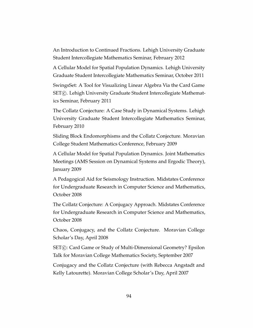
An Introduction to Continued Fractions. Lehigh University Graduate

Student Intercollegiate Mathematics Seminar, February 2012

A Cellular Model for Spatial Population Dynamics. Lehigh University

Graduate Student Intercollegiate Mathematics Seminar, October 2011

SwingsSet: A Tool for Visualizing Linear Algebra Via the Card Game

SET c©. Lehigh University Graduate Student Intercollegiate Mathemat-

ics Seminar, February 2011

The Collatz Conjecture: A Case Study in Dynamical Systems. Lehigh

University Graduate Student Intercollegiate Mathematics Seminar,

February 2010

Sliding Block Endomorphisms and the Collatz Conjecture. Moravian

College Student Mathematics Conference, February 2009

A Cellular Model for Spatial Population Dynamics. Joint Mathematics

Meetings (AMS Session on Dynamical Systems and Ergodic Theory),

January 2009

A Pedagogical Aid for Seismology Instruction. Midstates Conference

for Undergraduate Research in Computer Science and Mathematics,

October 2008

The Collatz Conjecture: A Conjugacy Approach. Midstates Conference

for Undergraduate Research in Computer Science and Mathematics,

October 2008

Chaos, Conjugacy, and the Collatz Conjecture. Moravian College

Scholar’s Day, April 2008

SET c©: Card Game or Study of Multi-Dimensional Geometry? Epsilon

Talk for Moravian College Mathematics Society, September 2007

Conjugacy and the Collatz Conjecture (with Rebecca Angstadt and

Kelly Latourette). Moravian College Scholar’s Day, April 2007

94

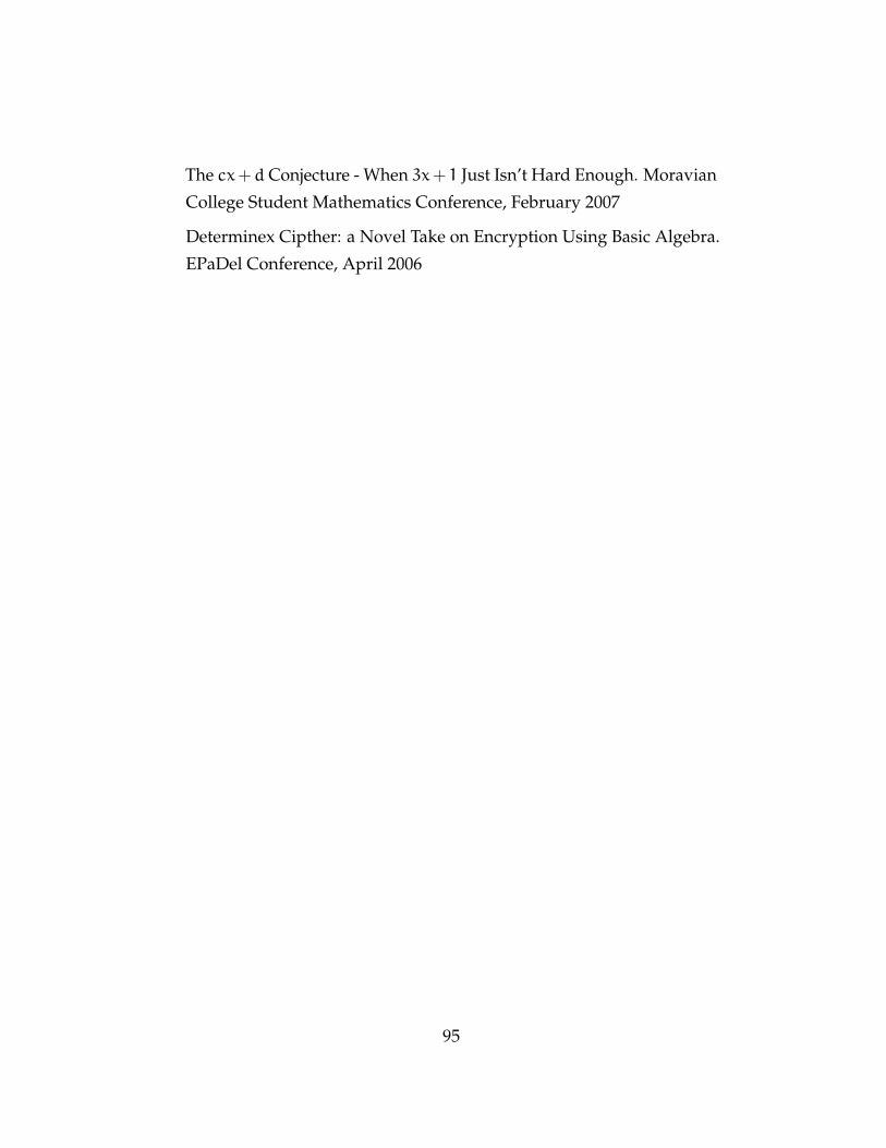
The cx+d Conjecture - When 3x+ 1 Just Isn’t Hard Enough. Moravian

College Student Mathematics Conference, February 2007

Determinex Cipther: a Novel Take on Encryption Using Basic Algebra.

EPaDel Conference, April 2006

95