Embed Size (px)
Citation preview

Carnegie Mellon University
Andrew, Chang, Eunice Choi, Diego Olalde, Kiran Thapa
21 393 - Fall 2016
Capacitated Facility Allocation withAutonomous Vehicles
1 Introduction
Valued at $62.5 billion now, who knew that Uber, when it was founded in 2009, would turn the
transportation industry upside down. Once were we told to not get into cars with strangers, now
we’re requesting rides from them. Through the Uber app, users request a trip, from their current
location to their destination, the software then sends the closest Uber driver to the user to service the
trip. The application allows users to track just where the driver is, give ratings and transfer payments
to the driver. In locations where owning a vehicle is difficult (e.g cities, college campuses etc.), Uber
thrived due to it’s convenience, and soon it became a go-to way of getting from one place to another.
With over 8 million users, and 1.1 million drivers worldwide (as of January 2016), Uber is now looking
to scrap human drivers in favor of autonomous vehicles in order to become more efficient and more
profitable. Pittsburgh is the hub of this shift in the auto industry, as Uber partners with engineers from
our very own Carnegie Mellon University, and thus naturally we chose this to be our topic of research.
As we began to discuss the developments of the self driving cars, we found ourselves wondering how
Uber would be able to coordinate the cars between users, where they would store these cars, and
just how much could they increase their revenue by and the challenges they would face. The main
challenge that we found to be of particular importance was the optimal geographical distribution of
facilities where the cars would be stores around a city to hold self driving cars in order to minimize
costs to Uber, and so we used this as our starting point.
2 Objective
Using Pittsburgh as our reference city, we wanted to create a model that would optimally locate fa-
cilities holding the autonomous vehicles in order to minimize the costs associated with storing and
operating the vehicles (dispatching, servicing trips etc.) and improve efficiency, taking into consider-
ation a multitude of real world constraints.
1

As of July 2016, Uber reported that it completed two billion rides, only six months after it completed
its’ first billion. This rapid (and increasing rate of) expansion of Uber, in only 7 years, reflects the
importance of our objective. By minimizing the costs to Uber, not only could Uber increase it’s profit
margins, but Uber would become more competitive, meaning lower fares passed on to users, (keeping
in mind that Uber has over 8 million users, a lot of money would be saved). By improving efficiency
(by minimizing the cost associated with dispatching and servicing cars as a function of distance and
time), we could save the time of Uber users, cars would be able to stay in service for much longer (due
to a slower depreciation of resources) and fewer cars would be on the road, meaning less congestion.
3 Model
3.1 Initial Model
We started off by simplifying the problem we wanted to solve to first assess if it could even be solvable;
and so we started with the very basic idea that if we had some points (i.e clients), where would we
locate a facility so that distance could be minimized. From this we would be able to define cost as a
function of distance. Doing some research into facility allocation, we came across the Uncapacitated
Facility Allocation Problem (UFAP), which very closely resembled our basic idea, and so we decided
to adapt the Uncapacitated Facility Allocation Problem to our topic. The Uncapacitated Facility
Allocation Problem locates a number (undetermined) of facilities to minimize the sum of the fixed
costs (costs associated with setting up the facility) and the variable costs (those costs associated with
serving the market demand from these facilities. This problem assumes that both client locations and
facility locations are discrete points and that client demand is concentrated at that point.
Given the following:
Variables
I : set of clients
J : set of facilities
2
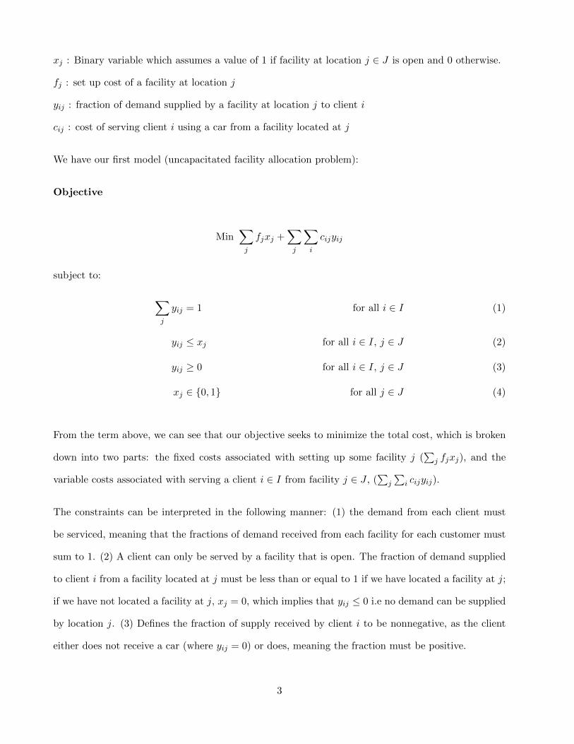
xj : Binary variable which assumes a value of 1 if facility at location j ∈ J is open and 0 otherwise.
fj : set up cost of a facility at location j
yij : fraction of demand supplied by a facility at location j to client i
cij : cost of serving client i using a car from a facility located at j
We have our first model (uncapacitated facility allocation problem):
Objective
Min∑j
fjxj +∑j
∑i
cijyij
subject to:
∑j
yij = 1 for all i ∈ I (1)
yij ≤ xj for all i ∈ I, j ∈ J (2)
yij ≥ 0 for all i ∈ I, j ∈ J (3)
xj ∈ {0, 1} for all j ∈ J (4)
From the term above, we can see that our objective seeks to minimize the total cost, which is broken
down into two parts: the fixed costs associated with setting up some facility j (∑
j fjxj), and the
variable costs associated with serving a client i ∈ I from facility j ∈ J , (∑
j
∑i cijyij).
The constraints can be interpreted in the following manner: (1) the demand from each client must
be serviced, meaning that the fractions of demand received from each facility for each customer must
sum to 1. (2) A client can only be served by a facility that is open. The fraction of demand supplied
to client i from a facility located at j must be less than or equal to 1 if we have located a facility at j;
if we have not located a facility at j, xj = 0, which implies that yij ≤ 0 i.e no demand can be supplied
by location j. (3) Defines the fraction of supply received by client i to be nonnegative, as the client
either does not receive a car (where yij = 0) or does, meaning the fraction must be positive.
3

3.2 Second Model - Capacities and Pairwise Demand
Let K denote a set of alternative facility locations, indexed by k. I denote a set of client locations,
indexed by i. This model seeks a subset of K that will satisfy the pairwise demands between all clients
i ∈ I.
This model was a good starting point as it provided a basic foundation upon which we could build
on and it helped us comprehend the components of our problem and form a general understanding,
however, it is not realistic as it does not take into account any real data or constraints such as facility
capacity, or the way dispatching would be carried out.
Variables
xkc : Binary variable which assumes a value of 1 if facility at location k ∈ K of capacity c is open and
0 otherwise.
yijk : Proportion of cars from facility K being sent to cover path from client i to client j, for i, j ∈ I.
fkc : cost of opening facility of capacity c at location k ∈ K.
lij : Demand from client i to client j, for i, j ∈ I.
dijk : distance covered by car starting at facility k ∈ K to go from i to j, for i, j ∈ I.
α : normalizing constant to represent the cost of traveling estimated distance over total time period
covered in model.
In the model it is assumed that fkc, lij and dijk are known and thus a solver would attempt to find
optimal assignment of xkc and yijk.
Objective
Minimize: ∑k,c
xkc · fkc + α ·∑k,j,i,c
(yijk · xkc · c) · dijk
4

subject to:
yijk ≤∑c
xkc for all (i, j, k) (5)
lij ≤∑k
(yijk ·∑c
cxkc) for all (i, j) (6)
∑c
xkc ≤ 1 for all k (7)
∑i,j
yijk ≤ 1 for all k (8)
yijk ∈ [0, 1], xkc ∈ {0, 1}
The objective function represents the total fixed and variable costs. Where fixed costs are determined
by summing up the total cost of opening facilities across selected locations and the variable costs are
estimated by the normalized dollar cost of the total distance covered by cars servicing client locations.
The normalization is determined by the value of α.
The constraints can be interpreted in the following way: (1) Closed facilities provide no service. (2)
Pairwise demand between every two locations is satisfied. (3) Only one facility is open per location.
(4) Each facility has maximum capacity.
This model is more appropriate than the Initial Model given that it now takes into account the
capacities, i.e facilities can only hold a limited number of cars, thus yielding a Capacitated Facility
Allocation Problem. Additionally, it more closely models the way in which Uber cars operate. Clients
requiring Uber’s service are not a facility at a fixed location, and this model attempts represent the
servicing of the pairwise flow between locations, which would represent the flow of cars between areas
of the city.
5

3.3 Final Model - Time and Excess Supply
Let K denote a set of alternative facility locations, indexed by k. I denote a set of client locations,
indexed by i, and T an ordered set of time intervals, indexed by t. This model seeks a subset of K
that will satisfy the pairwise demands between all clients I for all times T and minimize the total cost
in doing so.
Variables
nc: number of cars a facility of capacity c can hold.
xkc: binary variable indicating if facility k ∈ K of capacity c is open.
fk: unit cost of holding one car at facility k ∈ K.
Yikt: number of cars going from facility k ∈ K to client i ∈ I at time t ∈ T .
Wikt: number of cars going from client i ∈ I to facility kinK at time t ∈ T .
dik: distance between client i ∈ I and facility k ∈ K.
α : normalizing constant to represent the cost of traveling estimated distance over total time period
covered in model.
In the model it is assumed that fkc, lij and dik are known and thus a solver would attempt to find
optimal assignment of xkc, Yikt and Wikt.
Objective
Minimize:
∑k,c
nc · xkc · fk + α ·∑t
∑i,k
(Yikt +Wikt) · dik
6

subject to:
∑c
xkc ≤ 1 for all k (9)
∑k
Wikt = sit + Yikt −∑j
lijt for all (i, t) (10)
∑j
lijt ≤ sit +∑k
Yikt for all (i, t) (11)
∑ikt
Yikt =∑ikt
Wikt (12)
rkt ≤∑c
xkcnc for all (k, t) (13)
Wiktfinal≤
∑c
ncxkc for all (i, k) (14)
0 ≤Wikt for all (i, k, t) (15)
0 ≤ Yikt for all (i, k, t) (16)
Wikt ∈ Z+, Yikt ∈ Z+, xkc ∈ {0, 1}
where:
siti =
ti∑t=0
(∑k
Yikt −Wikt +∑j
ljit − lijt)
rkti =∑c
xkcnc +
ti∑t=0
∑i
(Wikt − Yikt)
The objective function represents the total cost as in the previous model. The main difference being
that in this model it takes into account the total cost across all time units, thus allowing a more
realistic simulation of how cars move throughout a city in a day to service varying demand.
Following is one possible interpretation of each of the constraints that the model presents: First notice
that sit represents the starting number of cars at client location i at time t and rkt represents the
starting number of cars at facility k at time t. (1) Only one facility is open per location. (2) At
every time unit unused cars at a location return to open facilities. (3) At every time unit the pairwise
7

demand between every two locations is satisfied. (4) All cars go back to some facility at the end of the
day. (5) At every time unit a facility can not hold more cars than its capacity. (6) At final time unit,
clients only return to open locations. (7) Non-negaive number of cars must be sent from facilities to
clients. (8) Non-negative number of cars must be sent from clients to facilities.
The model stipulates that initially, at t = 0, every facility is filled up to its capacity and every
client location is empty. Additionally, the above model only makes sense if the following ordering
assumption is made about the way the following events occur for each unit of time. For every time
t ∈ T , each facility k has an initial number of vehicles (rkt) and each client i has an initial number of
available vehicles (sit) along with a pairwise demand with every other client (lij). Once this has been
established, the cars initially available at every client location i, are used to satisfied the demand of
cars going from it, to every other client location. If at client i the demand is greater than the supply
of cars (∑
j lijt ≥ sit), then the open facilities send cars to client i (Yikt). Otherwise, if there is an
excess supply of cars (∑
j lijt ≤ sit), then excess cars are sent back to facilities (Wikt).
Besides the ordering assumption described above, the following are other important suppositions made
in the model. It is assumed that at any given time, excessive cars at some client location will return
to some facility, instead of possibly going to a nearby client location and servicing its excess demand.
In contrast to the previous model, distance is accounted as a cost only when the cars are traveling
without a client, i.e the distance of the path from a facility to a client or from a client to a facility.
The reason for this is that it is assumed millage costs are included into the service charge to riders
while the car is traveling between client locations. The model also assumes linearity of costs regarding
the cost of having one car at a given location (fk), ignoring economies of scale. It is also important
to point out that this model assumes that each unit of demand represents a distinct need for an Uber
trip, from a distinct car, thus it excludes the possibility of taking services like Uber Pool into account.
Finally there are is two important aspects of this model to notice. This first one being the value of
α, the constant that normalizes variable costs to make them yield a proper objective function value
when combined with the fixed costs. The value of α should be set to allow the comparison of the
8

cost of distance traveled to the cost of opening and maintaining a facility. For example, if we assume
that fixed costs are incurred on once per month (i.e rent), then α should be used to estimate the total
monthly cost of the total distance traveled in the model, in the subsequent sections we will cater to this
issue in more detail. The second one being the set T . When attempting to find an optimal solution
using this model it is vital to choose time units that are large enough to incorporate the sequence of
events previously described, but small enough to allow an adequate representation of the variability
of demand throughout the service period.
4 Data and Analysis
Due to the complexity of the final model, we decided to use proffesional level software in order to
find or approximate an optimal solution. It is for this reason that we decided to use Gurobi with
Python. Python is a high level yet powerful and flexible programming language that allows for rapid
and iterative program creation and Gurobi is a general purpose math programming solver. Thus, by
using Gurobi’s Python module we were able to create a smooth pipeline between coming up with
theoretical models, generating them and then testing their coherence. In the case of the particular
problem that we set up for Gurobi’s Solver, it found an optimal solution by a using branch-and-cut
algorithmm.
Before running the solver with real data, we ran it with made up data, i.e we generate a grid with
made up facility and client locations, demands between clients, as well as costs for the facilities. In
the figure below, we see a visualization of how our model provides a representation of one time unit.
The squares represent facilities and the circles represent client locations. The blue arrows represent
the supply of cars deployed from the facilities to clients, whereas the red arrows represent the cars
sent back to the facilities due to excessive supply within the client web. The black arrows represent
the pairwise supply and demand between the clients.
9

(The graphical representaiton of the model presented above was created using Python’s TK-
Inter, code is present in Appendix)
Once the model was feasible, coherent and all necessary constraints were accounted for, we were able
to move to the final part of our project, which was to determine how our model would work with real
life data that a company, like Uber, would use to make their decisions.
We proceeded to achieve one aspect of this goal by utilizing Google Map’s API to get realistic dis-
tance data that we could use within our model’s implementation. Specifically, we used Google Map’s
Distance Matrix API to extract actual driving distances between specific locations within Pittsburgh.
We used a python wrapper for the API to keep our work as streamlined as possible. In order to utilize
this real-life data within our model, we created a grid space overlay for the entire city of Pittsburgh
using the coordinates 40.4406 N, 79.9959 W as our centroid (this is the center of Pittsburgh). This
grid gave us a fair representation of how the ”nodes” within our model would be spread within the
city. The distance matrix that was provided was also an accurate representation of a distance cost
within the model. Below is an example of a small prototype 3 x 3 grid overlay above Pittsburgh with
a constant distance of 0.01 space (coordinate unit, equivalent to about 0.6 miles). The figure below
displays how our model would look when configured with Google Map’s data. We must to point out
that a realistic positioning of where the facilities and clients could be placed is not represented here,
10

but it shows that our model is capable of working with any sort of positioning, including realistic
input.
In order to make this model give a truly realistic solution, it would be necessary to know the following
data about Pittsburgh: relative cost between different areas in the city, demand of cars between each
area in the city, the cost of building a storage facility for self-driving cars, the estimated cost per mile
for a self-driving car and the availability of commercial locations to build storage space for self driving
cars. Hence due to the amount of data that we needed to gather in order to come up with a guess
estimate solution to our problem, we decided to take a different approach. We focused in using our
model to perform sensitivity analysis on the value of α. This would in turn allow us to understand
how important it would be to find an accurate representation of α when actually executing the model
to make a business decision.
The following assumptions where made during testing: all areas within Pittsburgh have the same cost
per square foot to open a facility in which to hold cars, demand from one location to another comes
from a uniform distribution between 0 and 5 for each time unit, each facility has a capacity for 100 cars
,Pittsburgh is divided in a 3 by 3 grid with 9 possible client and facility locations. This assumption
allowed the analysis of how the value of α would affect the outcome of the model.
11

Before testing we needed to figure out one additional factor, an initial sensible value for α. Currently it
is estimated that the cost per mile of driving for a car is 60 cents including gas, insurance, depreciation
and maintenance. Furthermore, alpha must account for time. The reason being that the way the model
is set up, it is running for a period of 24 time units, where each time unit represents 1 hour. Thus
the total distance calculated by the model will be the total distance traveled by cars for a period of
24 hours, but fixed costs are incurred on only once upon buying and building the facility, not every
24 hours. Hence α must also factor in this observation.
Assuming that fixed costs are only incurred upon every 4 years, or 1825 time units and that fk = 1
(i.e the cost of making a facility that holds 1 car for 5 years is 10, 000 dollars), along with the
aforementioned remarks, we choose the following value for α:
α = 0.6 ∗ 2000/10, 000 = 0.12. (Note: the value of α is rescaled by a factor of 10, 000 given that lk is
also rescaled by a factor of 10, 000 to make it 1).
Also note that the above value is just a rough initial starting point to allow for the sensitivity analysis
to get started. The table bellow shows the results of running the model with α values ranging from
0.05 to 0.55 with an interval of 0.05. We not only look at the cost that the objective function outputs
but we look at the facilities that it chooses, since the whole idea behind the model is to determine
which facility locations are ideal:
12

The results on the table seem to contradict our initial assumption that the model would be sensible
to the value of α. Note that even though the expected cost increase as α increases (this is totally
logical), the assignment of facilities does not change, in fact, the assignment of facilities was exactly
the same for all α. Do note that these tables do not include the sizes of facilities, which also remained
around the same for different α values.
This led us to believe that then reason all facilities where getting established was because otherwise
demand would not be fully satisfied, given that, if there are 9 client locations there is a total of 63
demand edges each with a maximum value of 5, which would cause a maximum demand of 315 units
of demand, or 1/3 of the total capacity. Thus we re-ran the model with very large capacities for
facilities, and the results remained the same.
In conclusion, given the above assumptions, it seems that the value of α will not affect the assignment
of facilities, but it will affect the total cost. It is also important to point out that we hypothesize that
the reason all facilities where determined to be opened by the model is that part of the assumption
was that they all had equal cost fk per car. The reason for this hypothesis is that when the model
was run with different cost per location using dummy data, only a subset of facilities was selected.
Hence, it seems that one of the primary factors to take into account when choosing facilities to locate
Uber’s self driving cars will be the cost of opening a facility in the area.
13

5 Further Improvements
Running the model with the data we had available left us with more questions than answers, thus
when considering the next steps, the obvious first choice would be to further improve the quality of the
data used to run the model. More specifically, it would be useful to work with true demand for each
time of the day and between each location. This would significantly change the assignment results for
facilities, since the flow would not be uniform like it currently is. Additionally, it would be very useful
to work with facility costs that are truly representative of the cost of opening a facility in the area,
this factor would also break the current symmetry of the nodes in the solution.
Furthermore, in the model it is assumed that cars that are not needed at one client location
will go back to the some facility, we believe that improving this assumption would highly improve the
quality of the model, given that costs of traveling to and from facilities would be further reduced.
We believe that these would be the most relevant improvements that could be made to the
current model to make it truly representative of Uber’s facility allocation problem.
14
6 References
Overview of what Facility Location Problems:
https : //optimization.mccormick.northwestern.edu/index.php/Facilitylocationproblems
Facility Location Problem Lecture:
http : //www.cs.cmu.edu/ anupamg/adv − approx/lecture4.pdf
Facility Location Problem Publication:
http : //onlinelibrary.wiley.com/doi/10.1111/j.1538− 4632.1987.tb00133.x/pdf
Springer, Chapter 2: Uncapacitated and Capacitated Facility Location Problems
7 Appendix
Code
The following code is the one used to create the mathematical model described above with Gurobi’s
Python module:
from gurobipy import *
import math
import numpy
from random import randint
#This section declares all model constant values
#Element i indicates the (x,y) location of client i
clients = [(100, 110), (120, 388), (413, 180), (500, 520)]
15

#Element i indicates the (x,y) location of facility i
facilities = [(50, 75), (50, 255), (200, 215), (400, 300),
(510, 65), (100, 450), (340, 50), (490, 350), (500, 500)]
#Element i indicates the cost of opening a facility of size 1 at location i
facilityUnitCosts = [1, 2, 4, 5, 1, 2, 1.5, 2, 3]
#Usefull values
numFacilities = len(facilities)
numClients = len(clients)
#Data structures to hold the model variables and constants
x = {}; n = {}; f = {}; y = {}; w = {}; l = {}; d = {}
#Number of possible different capacities for a facility
facilityCapacities = 30
# When multiplied by facility-capacity value, returns the number of cars that the
facility can hold. i.e
# if the capacity is 7, then the number of cars the facility can hold is
7*capacityMultiplier
capacityMultiplier = 10
#Total number of time units the model will run for
totalTime = 24
#Ratio of distance to facility cost in objective function
alpha = 0.5
#Given the index of a capacity, returns the number of cars that that a facility of that
#capacity can hold.
16

def capacity(c):
return capacityMultiplier * c
#Calculates the distance of the path a -> b
def distance((x0, y0), (x1, y1)):
dx = x0 - x1
dy = y0 - y1
return math.sqrt(dx * dx + dy * dy)
#Returns the demand of cars going from client i to client j at time t.
def demand(i, j, t):
if (t >= totalTime - 1): return 0
else: return randint(0, 100)
#START MODEL
# This function is responsible for adding all the variables and constants that will be used
# by the model
def addVariables(m):
#Variable X[k,c] binary variable which indicates if facility k of capacity c is open
for k in xrange(numFacilities):
for c in xrange(facilityCapacities):
x[(k, c)] = m.addVar(vtype=GRB.BINARY, name="X_%d,%d" % (k, c))
for c in xrange(facilityCapacities):
#Variable indicating the number of cars that a facility of capacity c can hold
n[c] = capacity(c)
17

for k in xrange(numFacilities):
#Variable f[k] cost of holding 1 car at facility k.
f[k] = facilityUnitCosts[k]
for t in xrange(totalTime):
for i in xrange(numClients):
for k in xrange(numFacilities):
#Variable Y_(i,k,t) variable indicating number of cars that facility k sends to client i
#at time t.
y[(i,k,t)] = m.addVar(lb=0, vtype=GRB.INTEGER, name="Y_%d,%d,%d" % (i,k,t))
#Variable W_(i,k,t) variable indicating number of cars that client i sends to facility k
#at time t.
w[(i,k,t)] = m.addVar(lb=0, vtype=GRB.INTEGER, name="W_%d,%d,%d" % (i,k,t))
for i in xrange(numClients):
for j in xrange(numClients):
for t in xrange(totalTime):
#Demand of cars needing to go from i to j at time t
l[(i, j, t)] = demand(i, k, t)
for i in xrange(numClients):
for k in xrange(numFacilities):
#Variable d_(i,k,j) indicates the distance of the path starting at facility k,
#going to client i
d[(i, k)] = distance(clients[i], facilities[k])
18

# This function is responsible for adding all the necessary constraints to the
# model
def addConstraints(m):
#Define two variables which will make constraints easier to understand
#Number of cars at location i at start time ti
def s(i, ti): return quicksum((y[(i,k,t)] - w[(i,k,t)])
for t in xrange(ti) for k in xrange(numFacilities)) +
quicksum((l[(j, i, t)] - l[(i, j, t)]) for t in xrange(ti)
for j in xrange(numClients))
#Number of clients at facility i start of time ti
def r(k, ti): return quicksum(n[c]*x[(k,c)]
for c in xrange(facilityCapacities)) +
quicksum((w[(i,k,t)] - y[(i,k,t)])
for t in xrange(ti) for i in xrange(numClients))
# Add constraints
for k in xrange(numFacilities):
#At most one size of a facility is open per location
m.addConstr(quicksum(x[(k,c)] for c in xrange(facilityCapacities)) <= 1)
for i in xrange(numClients):
#At final time, cars can only return to open facilities
m.addConstr(w[(i,k,totalTime - 1)] <= quicksum(n[c] * x[(k,c)] for
c in xrange(facilityCapacities)))
19

for t in xrange(totalTime):
for i in xrange(numClients):
#Excess cars at a given location go back to some facility
m.addConstr(quicksum(w[(i, k, t)] for k in xrange(numFacilities))
== (s(i, t) + quicksum(y[(i,k,t)] for k in xrange(numFacilities)) -
quicksum(l[(i,j,t)] for j in xrange(numClients))))
#Demand between all locations is satisfied
m.addConstr(quicksum(l[(i, j, t)] for j in xrange(numClients)) <=
quicksum(y[(i, k, t)] for k in xrange(numFacilities)) + s(i, t))
for t in xrange(totalTime):
for k in xrange(numFacilities):
#A facility can not send out more cars than it has at that time
m.addConstr(quicksum(y[(i, k, t)] for i in
xrange(numClients)) <= r(k, t))
#The number of cars at a facility must be less than its capacity
m.addConstr(r(k, t) <= quicksum(n[c] * x[(k,c)] for c in xrange(facilityCapacities)))
#All cars go back to some facility at the end of the day. Note that in order
for this to
be a viable constraint, we need to make the final unit of time
#have a demand of 0, such that cars can go back
m.addConstr(quicksum(y[(i, k, t)] - w[(i, k, t)] for t in xrange(totalTime)
for i
in xrange(numClients) for k in xrange(numFacilities)) == 0)
20

# This function is responsible for setting up the model and defining the objective
# function of the model
def startModel(model):
addVariables(model)
addConstraints(model)
model.setObjective(quicksum(n[c]*x[(k, c)]*f[k] for c in
xrange(facilityCapacities)
for k in xrange(numFacilities)) + alpha * quicksum(w[(i, k, t)] +
y[(i, k, t)] * d[(i, k)]
for i in xrange(numClients) for k in xrange(numFacilities)
for t in xrange(totalTime)) )
#NOTE: may need to multiply here by x[k, c]
def printResults(model):
vars = model.getVars()
for var in vars:
if(var.x != 0): print(var.varName + " = %.1f" % var.x)
def createTimeDict(d, md):
for (i, j, t) in md.keys():
var = md.get((i, j, t))
if (var != None and var.x != 0):
v = d.get(t)
if (v != None):
v.append((i, j, var.x))
else:
d[t] = [(i, j, var.x)]
21
def processResults():
facToLoc = {}; locToFac = {}
createTimeDict(facToLoc, y)
createTimeDict(locToFac, w)
return (facToLoc, locToFac)
#This function is responsible for setting up the model and invoking
#the Gurobi Optimizer on it.
# It returns tuple a, b, c, where:
# a : list of (k, c) where k is index of location and c is capactity,
#it only includes non-zero locations.
# b : dictionary (k, v) where k is the time unit and v is a list of
#tuples (x, y, z) which denote Y_(x, y, v) = z.
# c : dictionary (k, v) where k is the time unit and v is a list of
#tuples (x, y, z) which denote W_(x, y, v) = z.
def optimizeModel():
m = Model()
startModel(m)
m.ModelSense = GRB.MINIMIZE
m.optimize()
#printResults(m)
(b, c) = processResults()
a = [k for (k,l) in x if (x.get((k,l)).x != 0)]
return (a, b, c)
optimizeModel()
22

The following code used Python’s Tkinter to create an animation of the model’s results:
from Tkinter import *
from math import sqrt
import Tkinter as tk
import FacillityAllocationWithDemandsAndTime as FacAlloc
import time
facilityLocations = [(100,100),(100,300),(200,200),(200,300),(300,200),
(300,300)]
clientLocations = [(100,200),(200,100),(300,100)]
w = 40
class Facility(object):
def __init__(self, canvas, i, b, **kwargs):
self.canvas = canvas
(x0, y0) = facilityLocations[i]
self.x0 = x0
self.y0 = y0
self.color = "black" if b else "grey"
self.id = self.canvas.create_rectangle(x0, y0, x0 + w, y0 + w, outline = self.color)
self.text = self.canvas.create_text(x0 + w/2, y0 + w/2, text=str(i),
anchor = tk.CENTER, fill = self.color)
def updateText(self, newVal):
self.canvas.delete(self.text)
23

self.text = self.canvas.create_text(self.x0 + w/2, self.y0 + w/2, text=newVal,
anchor = tk.CENTER, fill = self.color)
class Client(object):
def __init__(self, canvas, i, **kwargs):
self.canvas = canvas
(x0, y0) = clientLocations[i]
self.id = self.canvas.create_oval(x0, y0, x0 + w, y0 + w)
self.x0 = x0
self.y0 = y0
self.text = self.canvas.create_text(x0 + w/2, y0 + w/2, text=str(i),
anchor = tk.CENTER)
def updateText(self, newVal):
self.canvas.delete(self.text)
self.text = self.canvas.create_text(self.x0 + w/2, self.y0 + w/2, text=newVal,
anchor = tk.CENTER)
class DemandLine(object):
def __init__(self, canvas, i, j, demand, **kwargs):
self.canvas = canvas
(x0, y0) = clientLocations[i]
(x1, y1) = clientLocations[j]
self.i = i
self.j = j
self.x0 = x0
self.x1 = x1
self.y0 = y0
24

self.y1 = y1
off = 0 if i < j else 8
if (x0 < x1):
self.id = self.canvas.create_line(x0 + w, y0 + w/2 + off, x1,
y1 + w/2 + off, **kwargs)
else:
self.id = self.canvas.create_line(x0, y0 + w/2 + off, x1 + w,
y1 + w/2 + off, **kwargs)
x_diff = x1 - x0; y_diff = y1 - y0
self.text = self.canvas.create_text(x0 + w/2+ x_diff/2,
y0+ w/2 + y_diff/2 + off, text= "", anchor = tk.CENTER)
def delete(self):
self.canvas.delete(self.id)
def updateText(self, time):
self.canvas.delete(self.text)
off = -5 if self.i < self.j else 5
x_diff = self.x1 - self.x0; y_diff = self.y1 - self.y0
val = FacAlloc.demand(self.i, self.j, time)
self.text = self.canvas.create_text(self.x0 + w/2+ x_diff/2,
self.y0+ w/2 + y_diff/2 + off, text= str(val), anchor = tk.CENTER)
class FlowLine(object):
def __init__(self, canvas, i, k, v, o, **kwargs):
self.canvas = canvas
25

(x0, y0) = clientLocations[i]
(x1, y1) = facilityLocations[k]
if (o == 1): off = 1
else: off = -1
self.id = self.canvas.create_line(x0 + w/2, y0 + w/2 + off,
x1 + w/2, y1 + w/2 + off, **kwargs)
def delete(self):
self.canvas.delete(self.id)
class App(object):
def __init__(self, master, **kwargs):
(self.xLoc, self.y, self.w) = FacAlloc.optimizeModel()
self.master = master
self.canvas = tk.Canvas(self.master, width = 600, height = 600)
self.canvas.pack()
self.time = 0
self.drawDemands()
self.createFacilities()
self.createClients()
self.canvas.pack()
self.master.after(0, self.animation)
def createFacilities(self):
self.facilities = [Facility(self.canvas, i, (1 if i in self.xLoc else 0))
for i in range(len(facilityLocations))]
26

def createClients(self):
self.clients = [Client(self.canvas, i) for i in range(len(clientLocations))]
def drawDemands(self):
self.currentDemands = [DemandLine(self.canvas, i, j, FacAlloc.demand(i, j, 0), arrow=tk.FIRST) for i in range(len(clientLocations))
for j in range(len(clientLocations)) if (i != j)]
def updateDemands(self, time):
for demand in self.currentDemands: demand.updateText(time)
def drawYIKT(self, time):
self.currentYIKT = []
if (self.y.get(time) != None):
for (i, k ,v) in self.y[time]:
self.currentYIKT.append(FlowLine(self.canvas, i, k, v, 1,
fill="blue", arrow=tk.FIRST, width = 2))
def drawWIKT(self, time):
self.currentWIKT = []
if (self.w.get(time) != None):
for (i, k , v) in self.w[time]:
self.currentWIKT.append(FlowLine(self.canvas, i, k, v, 0,
fill="red", arrow=tk.LAST, width = 2))
def animation(self):
currTime = self.time % 10
# if (time % self.step == 0):
# self.drawSIT(currTime)
27
if (currTime == 0):
self.updateDemands(self.time/10)
if (currTime == 3):
self.drawYIKT(self.time/10)
if (currTime == 6):
self.drawWIKT(self.time/10)
if (currTime == 9):
for line in self.currentYIKT:
line.delete()
for line in self.currentWIKT:
line.delete()
self.time += 1
self.master.after(300, self.animation)
root = tk.Tk()
app = App(root)
root.mainloop()
28