Marhemarical ModeNing, Vol. 7, pp. 443-448, 1986 Printed in the U.S.A. All rights reserved.

0270-0255/86 $3.00 + .oO Copyright Q 1986 Pergamon Journals Ltd.

CAPACITY REQUIREMENTS PLANNING BY STOCHASTIC LINEAR PROGRAMMING

T. C. E. CHENG

MBA Division Faculty of Business Administration Chinese University of Hong Kong

Shatin, NT, Hong Kong

Communicated by Ervin Y. Rodin

(Received January 1986)

Abstract-In this paper we formulate the problem of capacity requirements planning under uncertainty as a stochastic linear program (SLP). The objective is to minimize the total cost of underutilization, overtime production, and carrying inventory. Al- though it is desirable to achieve a stable inventory level in a production system, the stochastic nature of the demand causes inventory fluctuation over the planning ho- rizon. As a result, we incorporate in our model the deviation of the actual inventory level from the ideal inventory level as a set of chance constraints, which may be violated with a specified probability. In this way the SLP problem is transformed into an ordinary deterministic LP problem, which can be solved efficiently and cheaply on computers to obtain the optimal planning strategy.

INTRODUCTION

Effective capacity requirements planning is essential to production management since all other operation planning takes place within the framework set by the capacity plan. The primary objective of capacity requirements planning is the construction of a capacity plan for each work centre over a planning horizon to stabilize the planned lead-time (work-in- process inventory level). As unpredictable disturbances to a production system may occur from time to time which may lead to deviations of actual outcomes from planned outcomes, the planning procedure must be capable of dealing with this stochastic element in deter- mining the capacity plans for the work centres. In practice it will be extremely difficult, if not impossible, to eliminate completely the adverse effects induced by the occurrence of the random disturbances, such as exhausting of work-in-process inventory in a work centre caused by a sudden change in shipment plans. So it is assumed that management is prepared to accept a certain risk level that the undesirable disturbances will eventually take place.

Capacity plans are developed by first backward scheduling the released and planned orders by operations, then loading the work content of each operation into the work centre in which the operation will be performed in the appropriate time period, and finally totalling up the load from all operations in each time period for the individual work centres. Since this procedure is carried out without regard to the capacity limitations of the work centres, the resulting capacity plans for some of the work centres may be infeasible from a capacity point of view. Management is then required to take appropriate actions to alleviate the imbalance between capacity requirements and capacity availability by either rescheduling the master schedule so as to smooth out the loads imposed on the work centres (i.e. finite- capacity planning) or adjusting the capacity levels of the work centres from period to

443

444 T.C.E. CHENG

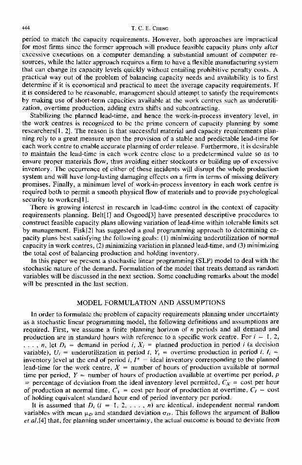
period to match the capacity requirements. However, both approaches are impractical for most firms since the former approach will produce feasible capacity plans only after excessive executions on a computer demanding a substantial amount of computer re- sources, while the latter approach requires a firm to have a flexible manufacturing system that can change its capacity levels quickly without entailing prohibitive penalty costs. A practical way out of the problem of balancing capacity needs and availability is to first determine if it is economical and practical to meet the average capacity requirements. If it is considered to be reasonable, management should attempt to satisfy the requirements by making use of short-term capacities available at the work centres such as underutili- zation, overtime production, adding extra shifts and subcontracting.

Stabilizing the planned lead-time, and hence the work-in-process inventory level, in the work centres is recognized to be the prime concern of capacity planning by some researchersil, 21. The reason is that successful material and capacity requirements plan- ning rely to a great measure upon the provision of a stable and predictable lead-time for each work centre to enable accurate planning of order release. Furthermore, it is desirable to maintain the lead-time in each work centre close to a predetermined value so as to ensure proper materials flow, thus avoiding either stockouts or building up of excessive inventory. The occurrence of either of these incidents will disrupt the whole production system and will have long-lasting damaging effects on a firm in terms of missing delivery promises. Finally, a minimum level of work-in-process inventory in each work centre is required both to permit a smooth physical flow of materials and to provide psychological security to workers[ 11.

There is growing interest in research in lead-time control in the context of capacity requirements planning. Belt[l] and Osgood[3] have presented descriptive procedures to construct feasible capacity plans allowing variation of lead-time within tolerable limits set by management. Fisk[2] has suggested a goal programming approach to determining ca- pacity plans best satisfying the following goals: (1) minimizing underutilization of normal capacity in work centres, (2) minimizing variation in planned lead-time, and (3) minimizing the total cost of balancing production and holding inventory.

In this paper we present a stochastic linear programming (SLP) model to deal with the stochastic nature of the demand. Formulation of the model that treats demand as random variables will be discussed in the next section. Some concluding remarks about the model will be presented in the last section.

MODEL FORMULATION AND ASSUMPTIONS

In order to formulate the problem of capacity requirements planning under uncertainty as a stochastic linear programming model, the following definitions and assumptions are required. First, we assume a finite planning horizon of IZ periods and all demand and production are in standard hours with reference to a specific work centre. For i = 1, 2, . . . ) n, let Di = demand in period i, Xi = planned production in period i (a decision variable), Vi = underutilization in period i, Yi = overtime production in period i, Zi = inventory level at the end of period i, Z * = ideal inventory corresponding to the planned lead-time for the work centre, X = number of hours of production available at normal time per period, Y = number of hours of production available at overtime per period, p = percentage of deviation from the ideal inventory level permitted, Cx = cost per hour of production at normal time, Cr = cost per hour of production at overtime, Cl = cost of holding equivalent standard hour end of period inventory per period.

It is assumed that Di (i = 1, 2, . . . , n) are identical, independent normal random variables with mean p,D and standard deviation (Tg. This follows the argument of Ballou et a/.[41 that, for planning under uncertainty, the actual outcome is bound to deviate from

Capacity requirements planning by stochastic linear programming 445

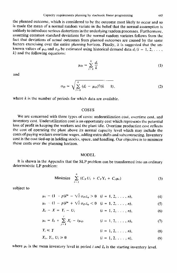
the planned outcome, which is considered to be the outcome most likely to occur and so is made the mean of a normal random variate in the belief that the normal assumption is unlikely to introduce serious distortions in the underlying random processes. Furthermore, assuming common standard deviations for the normal random variates follows from the fact that deviations of actual outcomes from planned outcomes are caused by the same factors exercising over the entire planning horizon. Finally, it is suggested that the un- known values of &, and (Tg be estimated using historical demand data di (i = 1, 2, . . . , k) and the following equations:

FD+

i= I

and

(1)

UD 1 J $, Cd - kD)'/(k - l), (2)

where k is the number of periods for which data are available.

COSTS

We are concerned with three types of costs: underutilization cost, overtime cost, and inventory cost. Underutilization cost is an opportunity cost which represents the potential loss of profit in keeping the workers and the plant idle. Overtime production cost reflects the cost of operating the plant above its normal capacity level which may include the costs of paying workers overtime wages, adding extra shifts and subcontracting. Inventory cost is the cost tied-up in holding stocks, space, and handling. Our objective is to minimize these costs over the planning horizon.

MODEL

It is shown in the Appendix that the SLP problem can be transformed into an ordinary deterministic LP problem:

Minimize $, (CX ui + CYYi + CIf-Li) (3)

subject to

pi - (1 - p)z* - vj uDZq > 0 (i = 1, 2, . . . , n), (4)

Pi - (1 - PP* + ti UDZ, < 0 (i = 1, 2, . . . , n), (5)

Xi - X = Yi - Ui (i = 1, 2, . . . , n), (6)

/k = 10 + 2 xj - ikD (i = 1, 2, . . . , n), j=l

(7)

Yi S Y (i= 1,2 ,..., n), (8)

Xi 9 Yi) Ui 2 0 (i = I, 2, . . . , n), (9)

where ki is the mean inventory level in period i and lo is the starting inventory level.

446 T. C. E. CHENG

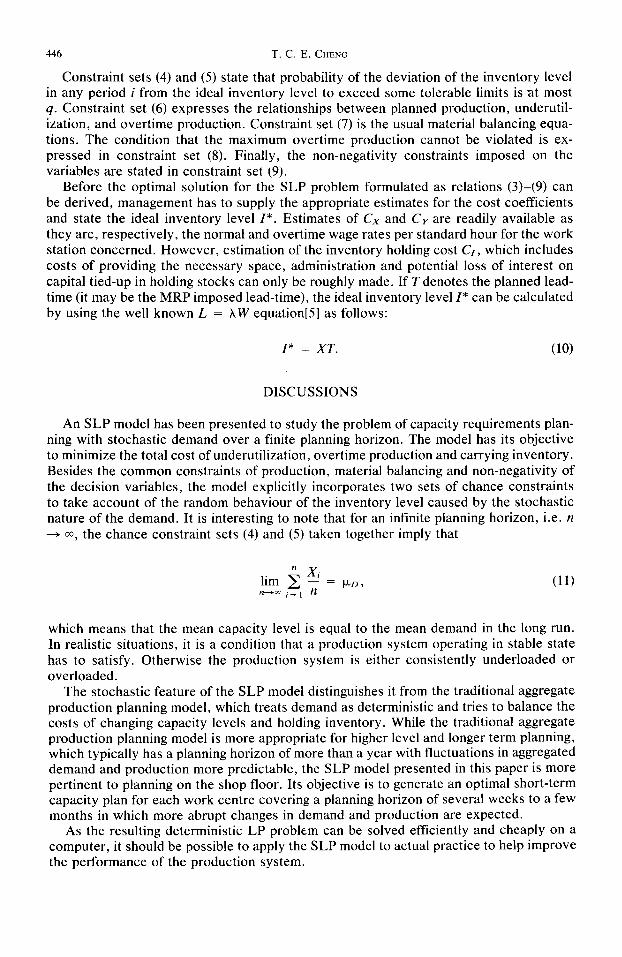
Constraint sets (4) and (5) state that probability of the deviation of the inventory level in any period i from the ideal inventory level to exceed some tolerable limits is at most 4. Constraint set (6) expresses the relationships between planned production, underutil- ization, and overtime production. Constraint set (7) is the usual material balancing equa- tions. The condition that the maximum overtime production cannot be violated is ex- pressed in constraint set (8). Finally, the non-negativity constraints imposed on the variables are stated in constraint set (9).

Before the optimal solution for the SLP problem formulated as relations (3)-(9) can be derived, management has to supply the appropriate estimates for the cost coefficients and state the ideal inventory level Z *. Estimates of CX and Cr are readily available as they are, respectively, the normal and overtime wage rates per standard hour for the work station concerned. However, estimation of the inventory holding cost C1, which includes costs of providing the necessary space, administration and potential loss of interest on capital tied-up in holding stocks can only be roughly made. If T denotes the planned lead- time (it may be the MRP imposed lead-time), the ideal inventory level Z* can be calculated by using the well known L = AW equation[5] as follows:

I* = XT. (10)

DISCUSSIONS

An SLP model has been presented to study the problem of capacity requirements plan- ning with stochastic demand over a finite planning horizon. The model has its objective to minimize the total cost of underutilization, overtime production and carrying inventory. Besides the common constraints of production, material balancing and non-negativity of the decision variables, the model explicitly incorporates two sets of chance constraints to take account of the random behaviour of the inventory level caused by the stochastic nature of the demand. It is interesting to note that for an infinite planning horizon, i.e. II + 00, the chance constraint sets (4) and (5) taken together imply that

(11)

which means that the mean capacity level is equal to the mean demand in the long run. In realistic situations, it is a condition that a production system operating in stable state has to satisfy. Otherwise the production system is either consistently underloaded or overloaded.

The stochastic feature of the SLP model distinguishes it from the traditional aggregate production planning model, which treats demand as deterministic and tries to balance the costs of changing capacity levels and holding inventory. While the traditional aggregate production planning model is more appropriate for higher level and longer term planning, which typically has a planning horizon of more than a year with fluctuations in aggregated demand and production more predictable, the SLP model presented in this paper is more pertinent to planning on the shop floor. Its objective is to generate an optimal short-term capacity plan for each work centre covering a planning horizon of several weeks to a few months in which more abrupt changes in demand and production are expected.

As the resulting deterministic LP problem can be solved efficiently and cheaply on a computer, it should be possible to apply the SLP model to actual practice to help improve the performance of the production system.

Capacity requirements planning by stochastic linear programming 447

REFERENCES

1. B. Belt, Integrating capacity planning and capacity control. Prod. & Invent. Mgmf 1, 9-16 (1976). 2. C. J. Fisk, A goal programming model for output planning. Decision Sci. 10, 593-611 (1979). 3. W. R. Osgood, How to Put the Output into Input/Output Control. Proc. 20th Annual Conf. American Prod.

& Invent. Control Sot.. Cleveland. Ohio. U.S.A. (1977). 4. D. P. Ballou, J. C. Fisk, and B. B. Ismail, Output planning for material requirements under uncertainty.

Omega 8,47-52 (1980). 5. J. D. C. Little, A proof of the queueing formula L = AW. Oper. Res. 9, 383-387 (1961).

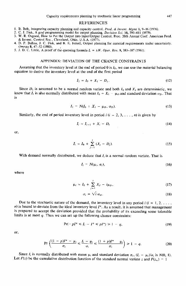
APPENDIX: DEVIATION OF THE CHANCE CONSTRAINTS

Assuming that the inventory level at the end of period 0 is lo, we can use the material balancing equation to derive the inventory level at the end of the first period

I, = lo + x1 - D,. (12)

Since D, is assumed to be a normal random variate and both I,, and Xi are deterministic, we know that I, is also normally distributed with mean lo + Xr - l&D and standard deviation UD . That is

II = N&l + xl - I*D, UD). (13)

Similarly, the end of period inventory level in period i (i = 2, 3, . . . , n) is given by

Z;=Zi_l +Xi-Di (14)

or,

Zi = lo + i (Xj - 0~). (15) j=l

With demand normally distributed, we deduce that Zi is a normal random variate. That is

where

fJ2i=IO+ iX,-ipD, (17) j=1

uj = duo,. w-9

Due to the stochastic nature of the demand, the inventory level in any period i (i = I, 2, . . . , n) is bound to deviate from the ideal inventory level I*. As a result, it is assumed that management is prepared to accept the deviation provided that the probability of its exceeding some tolerable limits is at most 4. Thus we can set up the following chance constraints:

Pr(-pZ* < Zi - I* GpZ*) 3 1 - 4, (19)

pr ( (1 - Plz* - CLi ~ Zi - Pi ~ (1 + PII* - Pi

ui ui ui > 2 I- 4. (20)

Since Zi is normally distributed with mean pi and standard deviation u;, (Zi - bi)loi is N(0, 1). Let F(z) be the cumulative distribution function of the standard normal variate z and F(z,) = 1 -

448 T.C. E. CHENG

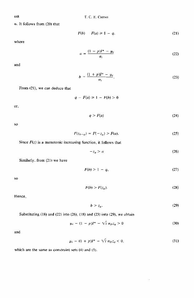
a. It follows from (20) that

F(b) - F(a) 2 1 - q,

where

a = (1 - PII* - lJ4

ui

and

b = t1 + Plz* - Pi

ui

From (21), we can deduce that

q - F(a) 2 1 - F(b) > 0

or,

4 > e)

so

F(z,-,) = F(-z,) > F(a).

Since F(z) is a monotonic increasing function, it follows that

-z, > a

Similarly, from (21) we have

SO

Hence,

F(b) > 1 - 4,

F(b) > Hz,).

b > z,.

Substituting (18) and (22) into (26), (18) and (23) into (29), we obtain

IJ-i - (1 - p)Z* - ti UDZq > 0

and

lJ,i - (1 + p)Z* + ti UDZq < 0,

which are the same as constraint sets (4) and (5).

(21)

(22)

(23)

(24)

(25)

(26)

(27)

(28)

(29)

(30)

(31)