Capillary forces and osmotic gradients in salt water - oil systems

Georg Ellila

Chemical Engineering and Biotechnology

Supervisor: Signe Kjelstrup, IKJ

Department of Chemistry

Submission date: June 2012

Norwegian University of Science and Technology

Preface

This master thesis has been carried out at The Department of Chemistry at TheNorwegian University of Science and Technology and in collaboration with StatoilASA. The report is a result of experimental work tougher with a related literaturestudy.

This is to my knowledge the first time the transport mechanisms in capillary oil-saltwater systems have been studied in detail, and therefor it was a lot of trail by errorin the beginning of the experiments. However, in the end I got quite comfortableby working with these small tubes and volumes.

There are numerous of people that have helped and supported me along my wayto and also through this thesis. In my mind, they all have a little piece in thisproject. Some more than others, but I am grateful for everything they have done.My family has always been supportive and encouraged me to do what I want, andnow I have accomplished one out of many things I want.

Signe Kjelstrup has been outstanding for me in this last year at NTNU, with herknowledge and always welcoming smile. The professor I feared to ask questions toduring the lectures in my 2nd year, has now become the person I prefer to ask forhelp. She has been curtail for me in the last year at NTNU, and for that I willalways be in grateful.

Kristian Sandengen and Statoil ASA have supported this project financially, andhave also been the creator of this project. I thank you for the support and I hopethe project can contribute to future work for Statoil and the Vista Program.

1

Abstract

This project looks at the capillary systems with salt water and oil that can be foundin porous stones in oil reservoir. The interactions between the different phases andhow salt concentration differences can move the oil. The first problem was to findhow the water migrates from one side of an oil droplet to the other due to theconcentration difference. This was discussed, but not experimentally verified. Thereason for this is the high inaccuracy of the experiments and the lack of knowledgebefore starting. However, this project gives a lot of important knowledge aboutthe problem, and good suggestions for improvements.

It was experimentally confirmed that oil is moving due to the difference in saltconcentration. From this, the diffusion coefficient was found and reported to beD = (1.08 ± 0.10) · 10−7m2

s for glass capillary tubes of radius 0, 70 mm and at60oC, calculated from the phenomenological coefficient L that was found. It wasalso confirmed that the capillary force does not contribute significantly for this sizeof the tubes, and therefore L should be independent of the radius.

The maybe most interesting result of the experiments and calculations is that thecapillary force will contribute significantly to the total force and then also themovement of the oil droplet. This does not happen before the radius of the tubeswhere under 0, 20 mm. The experiments and the estimates agreed well with theradius where the change happens.

2

Sammendrag (Norsk)

Denne masteroppgaven ble gjort for Instituttet for Kjemi ved NTNU i samarbeidmed Statoil ASA. Hensikten med forsøkene var å finne transportmekanismen forvann når det passerer olje inne i kapillarsystemer. I dette tilfellet ble det sett påoljedråper innesperret mellom vann faser med ulik natriumklorid konsentrasjon.Dette for å simulere om saltgradienter kan påvirke og forårsake bevegelse avoljedråper. Samtidig vil kapillarkrefter kunne spille en viktig rolle siden systemeneer svært små, med radius fra 0,13mm og opp til 0,70mm.

Kraften fra den osmotiske gradienten ble beregnet fra damptrykket til de ulike vannløsningene og er presentert i Tabell 5.1.1. Bidraget fra kapillarkreftene ble estimertpå bakgrunn av noen realistiske antagelser, som funksjon av menisk radiusen tiloljedråpen. Dette er presentert i Figur 5.2.1, mens den totale estimerte kraften erpresentert i Figur 5.5.2.

Det ble gjennomført flere forsøk hvor kapillarrørene var av samme type, men medulike saltkonsentrasjoner. Figur 2.1.1 viser en skisse av oppsettet med de ulikefasene indikert. Ved å la saltvannskonsentrasjonen variere kunne effekten fra denosmotiske gradienten vurderes og da også den fenomenologiske koeffisienten, seLikning 2.4.10 og Figur 5.3.1.

Det ble også gjennomført forsøk med tre forskjellige tykkelser på kapillarrørene;0,13mm, 0,26mm og 0,70mm. Dette for å kunne skille om vannet beveger seg langsmed veggene og dermed rundt oljedråpen, eller om det diffunderer igjennom. Ved åendre på rør tykkelsen og gjøre målingen av vannfluksen, vil man kunne se om den erproporsjonal med r, for bevegelse langs veggene, eller r2 for bulk diffusjon. Det varikke mulig å gi en konklusjon basert på resultatene fordi variasjonen av målingenevar svært høy og siden det burde vært gjort målinger ved flere ulike tykkelser pårørene for å gi en bedre regresjon av resultatene. Resultatet er presentert i Figur5.4.1.

For å finne ut om, eventuelt hvor mye, kapillarkreftene medvirker ble vannfluksenplottet mot radiusen. Dette skulle gi en rett linje med stigningstall 0 om ikkekapillarkreftene medvirket. Figur 5.5.1 viser dette plottet, og slik som tidligereestimert virker det som kapillarkreftene har en innvirkning når radiusen bli under0,20 mm.

Konklusjonen av prosjektet er at den osmotiske gradienten helt klart vil flyttepå oljedråper i kapillarsystemer, men også kapillarkreftene vil spille en rolle nårradiusen blir liten nok. Den nøyaktige overgangen vil nok variere litt, men bleestimert til å være rundt 0,20 mm. Andre mer praktisk relaterte spørsmål bleogså diskutert, som hvordan denne kan relateres til porøse kapillarsystemer ioljereservoar.

3

Contents1 Introduction 5

2 Theory 72.1 Description of the system . . . . . . . . . . . . . . . . . . . . . . . . 72.2 Chemical Potential . . . . . . . . . . . . . . . . . . . . . . . . . . . . 82.3 Surface tension and contact angles . . . . . . . . . . . . . . . . . . . 92.4 Driving Forces . . . . . . . . . . . . . . . . . . . . . . . . . . . . . . 152.5 Calculations . . . . . . . . . . . . . . . . . . . . . . . . . . . . . . . . 18

3 Experimental 233.1 The solutions . . . . . . . . . . . . . . . . . . . . . . . . . . . . . . . 233.2 Fluorecense effect . . . . . . . . . . . . . . . . . . . . . . . . . . . . . 233.3 Filling and measure the capillary tubes . . . . . . . . . . . . . . . . . 263.4 Accuracy and uncertainty . . . . . . . . . . . . . . . . . . . . . . . . 26

4 Observations 27

5 Results 285.1 Chemical potential . . . . . . . . . . . . . . . . . . . . . . . . . . . . 285.2 Capillary force . . . . . . . . . . . . . . . . . . . . . . . . . . . . . . 285.3 Movement of the oil droplet . . . . . . . . . . . . . . . . . . . . . . . 295.4 Transport mechanism . . . . . . . . . . . . . . . . . . . . . . . . . . 305.5 Distinguishing the two forces . . . . . . . . . . . . . . . . . . . . . . 31

6 Discussion 336.1 Theoretical estimates . . . . . . . . . . . . . . . . . . . . . . . . . . . 336.2 Does the osmotic gradient effect the oil movement? . . . . . . . . . . 346.3 What is the mechanism for the water migration? . . . . . . . . . . . 356.4 Will the capillary force contribute? . . . . . . . . . . . . . . . . . . . 36

7 Conclusion 37

8 Nomenclature 38

A Calculations of vapor pressure of water at 60oC 41

B Measurements 43

C Tabulated values for the calculations 45

4

1 Introduction

The aim of the project is to find out more about transport mechanisms and forcesin capillary salt water - oil systems. Why and how does the oil move in these smalland narrow systems?

The reason for studying these problems can easily be represented by money. Therecovery of an oil reservoir is rather low, normally from 20% up to 35% - 45% withthe use of secondary recovery1 [1]. The so called EOR2 can furthermore increasethe recovery to 60% [2]. The EOR is a general name for processes that changes thephysical and/or chemical properties in the reservoir to make it easier for the oil tocome out, and within this term is adding chemicals. One usually add chemicalsfor lowering the interfacial tension around the oil droplet, to make it move easier.This brings the problem back to this project, to find out more about the effect ofsodium chloride in the water that is in contact with the oil.

There has already been done experimental work on the effect of osmotic pressurein salt water/oil/water systems. Wen et al. [3] investigated how osmotic pressureinfluences the migration of water in double emulsion systems. In this case therewas a water bubble with low salt concentration that was almost in contact withanother high salt concentration water bubble of a greater size, just separated by ahydrophobic layer. Wen et al. observed that the low concentration bubble shrunk,meaning there was a migration of water from this bubble. This was happeninguntil the two bubbles had reached equilibrium, and the osmotic gradient was zero.By looking at the size of the bubbles before and at equilibrium together with theinitial concentrations, they could conclude that the salt does not migrate, onlywater. They also say that in equilibrium the bubbles have the same curvature.However, this is just transport through thin hydrophobic films and Wen et al.concluded that the migration is mainly via a hydrated surfactant mechanism. Thewater has no other way to leave the droplet than breaking down the film or diffusethrough according to Wen.

Cheng et al. made a study of how ions can transport through oil phase [4]. Thisagain is movement from one water droplet to another, but with an oil phase in-between. They had sodium chloride in one of the droplets and silver nitrate in theother, and observed if there was any sedimentation of silver chloride. They showedthat the thickness of the surfactant layer is critical for the transportation of ionsas micelles through the oil phase, with what seemed to be an optimum dependingon the ion that was transported. The Pauling radii was used to describe the sizeof the ions, and the large ions tended to move slower, likely because they needmore surfactants to create a micelle. They further stated that the transport rateof ions is independent of the thickness of the oil phase, with one exception whenthere is no visual oil phase between the two water droplets, just a double surfactantlayer. Then the transport was slower. The conclusion of the experiments is that

1Adding an artificial driving force when the natural pressure is too low2Enchanted oil recovery

5

there is a reverse micelle transport mechanism, where ions are surrounded by waterand then a surfactant layer is diffusing through the oil phase. The formation ofmicelles is the limiting factor for the transport, and water and/or ions do not breakthrough the surfactant layer and diffuse alone. This means that micelle formationis more important than the osmotic gradient for systems with surfactants at theinterface. Even though this is quite different from the system studied in this project,it is worth nothing that ions do not transport without being surrounded by thesurfactants, this will be assumed in the experiments for this project.

The force due to a chemical potential gradient is a strong force, so strong thatit can be used for a power plant, already done at Tofte in Norway, by the energycompany Statkraft [5]. The forces in capillary tubes are of course at a very differentmagnitude, but so are the required forces to move oil droplets as well. However, itis important to not forget the capillary forces, and at some point when the radiusis very small they will contribute. In this project I will look at both forces andseparate them by plotting the results.

This project is done on behalf of Statoil, one of the biggest actors in the oil industry,with the interest of learning more about the small and narrow systems inside theoil reservoir. Previously experiments conclude that osmotic gradients can lead tomigration of water, even through oil phase. The capillary force does not influencein these experiments, but for this project I will try to look at the magnitude of thecapillary force and the osmotic force together, to better understand how water canmigrate inside porous stones filled with oil.

6

2 Theory

The goal of the project is to answer the questions mentioned in the introduction;do osmotic gradients effect the movement? How does the water move? How willthe capillary force contribute? The upcoming subsections will go in more detailabout the physical properties and forces in a system like this, but first one has tolook at the actual case for this project.

2.1 Description of the system

To simulate the movements in a porous stone containing saltwater and oil, I havefilled capillary tubes with an organic compound and water of different salinity,Figure 2.1.1. The two phases a and e are the same water solutions, and bothare directly connected to the bulk phase around the tubes. In this way theconcentration can be assumed to be constant and the same for the two. Thehigh salinity phase in the middle, c, is also a water solution, but with higherconcentration of sodium chloride. This will create differences in chemical potentialand surface properties for c with respect to the other two water phases. The twooil droplets, b and d, separates the high salinity solution from the low. They canbe looked at as membranes that can be selective in the transport of molecules, alittle like the membranes used in osmotic power plants and fuel cells. One of thequestions for this project is how the oil phase is transported.

Figure 2.1.1: Sketch of the capillary tubes with letters assigned to the different phases

A setup like this will create forces that wish the oil droplets to move away fromeach other, assuming that the water migrates easier than the sodium chloride ionsas mention earlier. Also a capillary force could work in this direction. If one justmeasures a system like this it will be impossible to say what causes the movement.However, by doing series of experiments with small changes in the system it maybe possible to distinguish the two forces. Figure 2.1.2 shows the forces that play avital role in a system like this.

The first idea for distinguishing the two forces, has been to change the walls of thetube, which will only change the capillary forces. The weakness of this is that it

7

Figure 2.1.2: Sketch of the forces working on the droplet together with important variables thatis frequently used in this project

might change the mechanism as well. It is likely that the migration will be effectedif the walls were highly hydrophobic or hydrophilic. This is important to keep inmind when relating the results to an actual oil reservoir where the walls are madeof porous stone. Zhou et al. have studied the importance of wetting for the porousstones when it comes to oil recovery, and found it to be important [6]. However,they do not study the transport mechanism so it is impossible to say weather it isthe same for all the experiments or if it changes with different wetting conditions.

2.2 Chemical Potential

A part of the chemical potential can be compared to "a measure of the potentialthat a substance has to produce in order to alter a system" according to Atkins [7].It can be compared to other potential energies such as gravitational and electricalpotential energy that causes something to move because it is in a different energystate with a reference to something else. Mathematically it is dependent on alot of variables and therefore can be described as different partial derivatives, alldepending on what variables that are kept constant. For this project I want to varythe concentration and that is why I have chosen to define the chemical potentialfrom the Gibbs’ energy, Equation 2.2.1

µi =(∂G

∂ni

)T,P,nj 6=i

(2.2.1)

According to Atkins the Gibbs’ energy for a gas can be expressed as following,relative to the standard state at 1 bar [7].

G = nG0m +RT ln

(PvapP 0

)(2.2.2)

Where R and T are the universal gas constant and the temperature in Kelvinrespectively. Using Equation 2.2.1 and the fact that µvapor = µliquid for systemsthat are in equilibrium, one will get an equation that is more suitable for this

8

project, Equation 2.2.3. The pressure ratio can also be expressed in terms of theactivity Pvap/P 0 = ai, where Pvap is the vapor pressure for the solution and P 0

is the reference pressure, in this case for pure water. The activity is maybe morelogic to use for liquid-liquid systems, but there will always be a theoretical vaporpressure over a solution even though there is no gas phase.

µi = µoi +RT ln(ai) ⇒ ∆µi = RT ln(P2,vap

P1,vap

)(2.2.3)

The change in chemical potential, ∆µi, of the solvent when adding salt is usuallynegative and this is also the case for sodium chloride. The more one adds thelarger is the decrease in chemical potential [8]. An important thing to notice isthat the chemical potential difference depends on the temperature. This meansthat the force caused by chemical potential is getting larger just by increasingthe temperature, and the difference could be significant because it is directlyproportional to the temperature in kelvin. The temperature dependence of thepermeability is somehow still unknown and can also influence the movements.

The vapor pressure was found by calculation from the osmotic coefficients [9] [10].It should be mentioned that the osmotic coefficients were originally calculatedfrom the vapor pressure but the vapor pressure it self was not reported. Afurther description of the calculations can be found in Appendix A together withall data tabulated. Figure 2.2.1 shows the vapor pressure at different sodiumchloride concentration and Equation 2.2.4 is a regression of the plot, where c is theconcentration.

Pi,vap = 66, 664c2i − 2093, 6c1 + 19934 (2.2.4)

The plot goes all the way to the solubility limit of sodium chloride at a temperature60oC, and it is even valid for slightly over saturated solutions. This gives raise toa chemical potential difference of up to 1,62 kJ/mol, according to Equation 2.2.3.Table 5.1.1 shows the other chemical potential differences used in the experiments.

2.3 Surface tension and contact angles

A very important aspect in capillary systems is the interactions that happen atthe surface between the different phases. The systems in this project have differentsodium chloride solutions of various concentration, oil in form of octane and thewall of the capillary tube. For the individual surface tension of the liquids there aretwo main factors that contribute, namely dispersion forces and interaction forcesspecific for the different liquids, Equation 2.3.1. Another and more general namefor these forces is Lifschitz - van der Waals forces, and it includes all the forcesthat contributes to the surface tension [11].

9

Figure 2.2.1: Plot of the vapor pressure versus the sodium chloride concentration for solutions at60oC.

γ = γdisp + γsp (2.3.1)

The γsp term can for instance be due to hydrogen bonding like in the discussedsystem. For water and dilute water solutions the hydrogen bonding together withthe dispersion forces will be dominant, and other effects can be neglected. However,when the salt concentration increases also the salt ions contribute significantly tothe surface tension. Experiments show that the contribution of sodium chlorideions leads to an increase in the surface tension [12] [13].

For the octane phase it is more simple, because according to P. C. Mørk [11] thespecific forces can be neglected for non polar hydrocarbons and the total surfacetension is therefor equal to the contribution from the dispersion forces.

γsp = 0 ⇒ γoctane = γdisp (2.3.2)

Surface tension is usually measured when a liquid is in contact with a gas phase,normally air. The reason for this is that the influences to the surface tension ofthe liquid, that is caused by the air/gas, can be neglected and thereby one canmeasure surface tension for each individual substance alone. In other cases, likethis project, there is no gas phase, but rather two liquid and one solid phase. Thisis a more common systems in our everyday life, and in this case the surface tensionof a substance is then relative to what it is in contact with. Interfacial tension

10

is the term used for distinguishing between the two types of systems. Interfacialtension describes the same phenomena with the same laws of physics, but is usedfor liquid-liquid systems and will be used in this project. One rule is that theinterfacial tension will always be lower than the highest surface tension for theindividual substances in contact. Table 2.3.1 shows some of values that will be ofinterest for this project with some additional values that are useful for comparisons.It was said that for non polar hydrocarbons the surface tension was only dependenton the dispersion forces, but if an alcohol group is introduced, octanol, the surfacetension gets higher. This is most likely due to the possibility for hydrogen bonding,confirmed by the fact that it’s interfacial tension to water is lower than the surfacetension. Clearly there are some kind of bondings across the interface region thatmakes it weaker. The values in the table are for the substances at 20 ◦C, and ingeneral the surface tension decrease with increasing temperature [13].

Table 2.3.1: Tabulated values of surface tension and interfacial tension against water at 20◦C [11]

Liquid Surface Tension Interfacial Tension against[mN/m] water [mN/m]

Water 72.8 −Water solution(1.0MNaCl) 74, 4[13] −Water solution(2.7MNaCl) 77, 9[13] −

Octane 21.8 50.8Octanol 27.5 8.5Ethyleter 17.1 10.7

The interfacial tension can be estimated from Fawkes equation, 2.3.3. Thedispersion forces here contribute in a negative order to the interfacial tension whileother specific forces contribute in a positive order. This means that for instancethe hydrogen bondings in water will give raise to a high interfacial tension. Fromthe values in Table 2.3.1 it is possible to estimate how much the hydrogen bondingcontributes to the resulting interfacial tension for water-octane solutions, γdwater =22.0 mN/m and γspwater = 50.8 mN/m.

γAB = γA + γB − 2(γdA · γdB) 12 (2.3.3)

As already mentioned, water with sodium chloride ions have a higher surfacetension, and from Fawkes equation one can see that this will influence the interfacialtension between water and octane. It is worth noticing that adding sodium chloridewill change the γwater but it might change the γdwater as well. This means thechange in surface tension of water will not necessarily be the same as the change ininterfacial tension between water and another compound. It depends if the changein surface tension of water is caused by a change in the γd or γsp.

A more detailed description of the change in surface tension due to adding a solutecan be seen from the Gibbs adsorption isotherm equation. Before this is introduced,

11

it is necessary to define the surface excess, Γ. It can be looked at as a surfaceconcentration, so a two dimensional concentration on macroscopic level.

Γi = Nσi

A(2.3.4)

Where Nsigmai is the number of molecules and the denotation σ indicates that it

is on the surface, A is the surface area. The surface can be defined as the smallvolume where the concentrations are changing with respect to the bulk phase. Inthis region again one can place a plane without any volume, usually referred toas Gibbs’ dividing interface. The surface excess depends on where this plane isactually placed and is a very useful variable for describing a surface. Figure 2.3.1shows an example for a one component system with two phases, and Gibbs’ dividinginterface is defined such that Γ = 0 [14]. This is of course at a molecular level werethe distances are very small, but on a microscopic level the surface will look like aplane without any volume.

Figure 2.3.1: Ideal placement of the Gibbs dividing interface for one component system with twophases.

The surface line can be chosen freely, but for a single component system it is likelyto place it in the middle of the interfacial region. That is sometimes referred to asthe perfect surface because each of the phases have the same amount of molecules,within the interfacial region, on each side of the defined surface. For this kind ofsurface the surface excess is defined as zero, Γi = 0. Sometimes it is convenient dodefine the surface line differently and then the surface excess will be different fromzero, example Figure 2.3.2. This will be the relative adsorption, meaning that thesurface excess is relative to the other component(s) in the system, mathematicallyexpressed in Equation 2.3.5.

12

Γ(1)i ≡ Γσi − Γσ1

cαi − cβ1

cα1 − cβ1

(2.3.5)

Where the notations α, β and σ indicate the the bulk phase 1, bulk phase 2 andthe interfacial region of the system.

Figure 2.3.2: Two possible placements of the Gibbs dividing interface that makes the surfaceexcess different from 0

In this project it is a multi-component system with water, sodium chloride andoctane. When there is a solution with two components there will also be twocomponents present at the surface. Depending on how they interact with the otherphase, it might not be a continuous concentration drop in the interfacial zone forboth of the two components, an examples can be viewed in Figure 2.3.3. If therelative concentration profile in the interfacial region is different it will be impossibleto find a perfect surface line where Γi = 0 for both. This brings it back to Gibbsadsorption isotherm equation which says that the change in surface tension is alinear combination of the changes in chemical potential.

dγ = −∑

Γidµi ⇒ dγ = −Γwdµw − ΓNaCldµNaCl (2.3.6)

13

Figure 2.3.3: Example of a multicomponent system where a solute is enriched just under thesurface

The expression simplifies a lot by defining the surface so that the Γw = 0, meaningthat the surface is defined by the water concentration in the interfacial regionwithout thinking of the sodium chloride. Then taking the derivative of Equation2.2.3 and inserting it into Equation 2.3.6 gives the following equation.

Γ∗2 = − a

RT

∂γ

∂a

∣∣∣∣∣T

(2.3.7)

A very important equation which tells directly that solutes that enrich the surfacewill give a lower surface tension than the pure component and vice versa. As earliermentioned sodium chloride gives a higher surface tension, which means it does notenrich the surface. In reality there are two interfaces, one for the water and one forthe sodium chloride. It is normal for highly polar solutes such as ions to increasethe surface tension of water, while most other non-polar solutes will lower it [14].

The force due to surface tension is usually referred to as the capillary force. Forthis project I have chosen a little different approach starting out with the partialmolar pressure dependent Gibbs’ energy, Equation 2.3.8.

∂G1

∂P1= V1 (2.3.8)

In the system there will be a pressure difference from one side of the oil droplet tothe other. This is because the surface tension of the two water solutions will bedifferent and lead to different curvature of the meniscus. From Young-Laplace’sequation, 2.3.9 one can see that a different radius of the meniscus will lead to a

14

pressure difference that will be a contributing force to the movement of the oildroplet.

∆P = γiR1

+ γiR2

for R1 = R2 ∆P = 2γR

(2.3.9)

Where R is the radius of the menisci, and ∆P is the pressure difference overthe meniscus of one side of the oil droplet. A combination of Young-Laplaceequation for each of the sides, gives the pressure difference over the whole droplet.Integration of Equation 2.3.8 from one side of the meniscus to the other, and theuse of Young-Laplace equation, will give an expression of the free energy

∆G = Vm

(2γiR

)(2.3.10)

This equation will be usefull when describing how the capillary forces will contributeto the movement of the oil droplet. This will be further discussed in the upcomingsection together with the contribution from osmotic gradients.

In the end I want to introduce Young’s equation which gives a relation betweenthe surface tensions and the interfacial tension, Equation 2.3.11. It also relates thecontact angle to the different surface/interfacial tensions.

γsg − γsl = γlg cos(θ) (2.3.11)

2.4 Driving Forces

For this project I have chosen to look at the local entropy production, and definingthe local entropy production in the oil phase as the contribution from the capillaryforce. The movement is dependent on either the osmotic force, ∆µw, or thepressure difference cause by difference in interfacial tension and curvature, ∆µc,or a combination of the two. This gives two equations, but one must rememberthat the change in chemical potential and the capillary force are related. Meaningthat if one of them changes the other one will as well. The two equations bellowdescribe the local entropy production for the system

σw = Jw

(− 1T

dµwdx

)− JNaCl

(1T

dµNaCldx

)(2.4.1)

σo = Jw

(− 1T

dµcdx

)(2.4.2)

Where subscript w indicates water, o oil and c capillary force. Every sodium andchloride ion will be carrying some water molecules around due to their electrical

15

charge. This will slow down the movement and also prevent the ions from movingthrough or around the oil phase. For the project I have assumed that there is noflux of sodium chloride. This have been verified experimentally for a similar systemby Wen et al. [3]. If JNaCl is equal to 0 then the last term can be removed from theEquation 2.4.1. The entropy production defines fluxes, and their conjugate forces.And according to Onsager, the flux is proportional to the forces multiplied by aconstant [15]. Meaning that the water flux can be expressed as following

Jwater = −L 1T

(dµwdx

+ dµcdx

)(2.4.3)

Where L is the phenomenological coefficient. The total local entropy productionwill be the sum of the local entropy production equations 2.4.1 and 2.4.2 , and byintegration over the distance one will get the total irreversible entropy production.This will be the entropy production over one oil droplet.

Sirr

dt=∫ l

0σw + σodx = −Jw

1T

[µw,l − µw,h

δ+ ∆µc

δ

](2.4.4)

Where the µw,h and µw,l mean the chemical potential of water phases with highand low salinity respectively. This have been explained earlier and they can beexpressed according to the Gibbs’ equation 2.2.3.

The ∆µc is still unsolved and hard to estimate, but with use of the theory explainedin the previous section it is possible to expressed in terms of measurable variables.These kind of measurements requires apparatuses of high precision and thereby tooexpensive to use for this project. The equations can still be derived completely free.When the oil droplet is in contact with two surfaces with different surface tensions,there will be a constant difference in pressure at each side. One can look at thedifference in curvature and calculate the capillary force or simply just multiply thepressure difference with the molarity of the oil to get a force, which I have chosento call ∆µc.

∆µc = Vo[Po,h − Po,l] (2.4.5)

Where the two pressures in the oil are distinguished by h (high) and l (low) toindicate the concentrations in the surrounding solutions. Then by adding andsubtracting the pressure in the water phase, Pw, gives an equation with similaritiesto Young-Laplace equation 2.3.9.

∆µc = Vo[Po,h − Pw − Po,l + Pw] (2.4.6)

There are two pressure differences which are related to each of the curved interfacialsurfaces of the oil droplet, and therefore the Young-Laplace equation can be applied.However this equation is for spheres, tubes, droplets and other similar geometries.

16

In this project it is not the surface tension relative to the center of the curvature ofthe interfacial region, but its contribution to the movement along the walls. Thiswill be compensated by multiplying with the cosine to the contact angle, θ (seeFigure 2.1.2). So by combining Equation 2.3.9 and Equation 2.3.10 and includingthe cosine to the angle one get an equation for the capillary force.

∆µc = Vo

[2γw,h cos(θh)

rh− 2γw,l cos(θl)

rl

](2.4.7)

Where γw,i is the interfacial tension between the oil phase and the water for thedifferent concentrations, i. It can be written a little different with the use of Young’sequation 2.3.11.

∆µc = 2Vo[γo,s − γw,h,s

rh− γo,s − γw,l,s

rl

](2.4.8)

Where the last subscript s indicates that it is against the solid surface, in this caseglass. All of the surface tensions against solid are unknown, so it will be very hardto predict this force.

This brings the problem back to Equation 2.4.3, so the water flux can be expressedas following for migration from phase a to phase c. The very same situation willbe for the transport from e to c.

Ja = −L 1T

[∆µw + ∆µc

]1δb

(2.4.9)

δb is the thickness of oil droplet b. And to write the final expression including thesimplification mention earlier and the derivation done, it will gives this

Ja = −L 1T

[RT ln

(P2,vap

P1,vap

)+ 2Vo

{γo,s − γw,h,s

rh− γo,s − γw,l,s

rl

}]1δb

= −L 1T

∆µ(a→ c)δb

(2.4.10)

Looking at the final equation one can predict three different outcomes for theoil droplet depending on which direction the forces works. Letting the osmoticforce work in the positive direction, then depending on the interfacial tension thedroplet can move both ways or stand completely still. If µw = −µc there will be nomovement. To do so the Interfacial tension between the water solution and octaneneeds to be lowered when adding the solute. This can very well happen and formost compounds it will actually be true, except the one with strong ionic forces.This one will contribute in a positive way to the osmotic force and increase thetotal force.

17

The final equation can also be compared with Fick’s law J = −D dcdx . This will be

done to relate the results to a diffusion coefficient and thereby get a more practicalview of the results. The relation between the diffusion coefficient and L is rathereasy

L = DVwR

(2.4.11)

Where Vw is the concentration of pure water and D is the diffusion coefficient.

2.5 Calculations

The first and most important task is to find the transport mechanism of the water.Will the water diffuse through the oil phase or will it migrate along the wall of thetube? To distinguish the two mechanisms one needs to look at the determiningvariables for the speed of the oil droplet. Obviously the forces mentioned in theprevious subsections are important, but they are after all constant for each system.This is not completely true because the concentrations will change with time,because of the water transport, and so will the osmotic gradient and interfacialtension. However, for the calculations they are assumed to be negligible. Themovements can still differ from one capillary tube to another depending on sizeand material, and thereby lead to differences in the water flux. By comparingdifferent capillary tube systems, it is possible to answer the questions stated in thisproject.

Another factor that is important for the transport, or the speed of the oil droplet,is the length of the oil droplet together with the area or circumference. If themechanism is diffusional one have to look at the volume the water have to passthrough, while if the migration is along the walls one need to look at the area ofthe wall. The oil droplet can be assumed to have the shape of a cylinder, and thenthe volume is proportional to the radius squared, while the area of the wall is justproportional to the radius.

Flux equations and transport mechanism

The water flux is expressed as the mole change per time unit, divided by an area.In this case we want to see if the migration of water is dependent on the crosssectional area of the capillary tube or just the circumference of it, I will come backto this. The equations below show an expressions for the water flux where A is anarea. The two first ones are for each of the droplets, while the third is the totalwater flux, set to positive even though the two fluxes are in opposite directions.

Jw(a→ c) = 1A

∆naw∆t (2.5.1)

18

Jw(e→ c) = 1A

∆new∆t (2.5.2)

Jw = 1A∆t (∆n

aw + ∆new) (2.5.3)

In this case the A will be the cross sectional area of the capillary tube, πr2. Thisexpression can be set equal to the contributing forces earlier mentioned to get thewhole picture of the system.

For a more practical point of view, one can express the water flux as a volume flow,and then relate it to the actually measured speed of the oil droplet.

Jv = Jw(a→ c)Vw + Jw(e→ c)Vw (2.5.4)

Where Jv is the volume flux and Vw is molar volume. The dimensions of the volumeflux will be m3

m2s or just m/s. This means that the volume flow is directly relatedto the speed of the droplet which again can be expressed as

Jv = ∆VA∆t = ∆x

∆t = vaw + (−vew) (2.5.5)

Where ∆x is the change in distance between the droplets, which corresponds tothe sum of the movements of both droplets. The negative sign comes from the factthat the droplets are moving in the opposite direction. They will be separate waterfluxes and they can be expressed as the equations bellow as earlier mentioned.

Jw(a→ c) = −L 1T

∆µ(a→ c)δb

(2.5.6)

Jw(e→ c) = −L 1T

∆µ(e→ c)δd

(2.5.7)

In this case the two differences in chemical potential will be the same, but inopposite directions. When adding the two fluxes together it will only be thethickness of the oil droplet that differs.

Jw(a→ c) + [−Jw(e→ c)] = −L 1T

[δb + δdδbδd

]∆µ(a→ c) (2.5.8)

Instead of taking the average thickness over the two droplets one can be moreprecise and use the expression above for the thickness. The reason why I look atboth the water fluxes together is that, in some way, there is a correlation betweenthe movements of the two oil droplets. The distance between them is very small,

19

so it is likely to think the movements can influence each other a little. All themeasurements that are done will give directly a volume flux rather than the molarflux, for the molar fluxes I have assumed that it is 54,58 moles per liter of water at60o C.

The problem with this approach is that we look at the whole cross-sectional area ofthe tube no matter if the water transport is along the wall or diffusional, equation2.5.5. In reality the area where there is a transport of water will be a lot smallerif the migration happens along the wall, Figure 2.5.1 illustrates the problem.

Figure 2.5.1: The effective diffusional area for the two transport mechanisms, cross sectional cutof the capillary tube

With this in mind it is obvious that looking at a plot of the water flux against theradius will make it difficult to draw any conclusion from. However, by looking atthe amount of water passing from one side to another per time unit, V , will be alot better. This is easy to calculate and is not dependent on the radius of the tubein the same way as the water flux, Equation 2.5.9

V = πr2 ∆x∆t (2.5.9)

By plotting this volume flow against the radius of the capillary tubes for systemswith the same osmotic gradient, one should be able to distinguish if the flow isdependent on r or r2 and thereby the two different transport mechanisms. Figure2.5.2 shows an example of the plot with the two possibilities explained, withconstant osmotic force. It can of course be a mix of the two as well or otherpossibilities. If the system had any surfactant it could have been very differentagain. It is important to mention that this assumes that the capillary force isnegligible. If the capillary force contributes it will change the shape of the curvewhen it gets closer to zero.

20

Figure 2.5.2: Example graph for the two different transport mechanisms for constant force

The capillary force

The influence of the capillary force is, as mentioned earlier, very hard to distinguish.However it is possible with some assumptions. First I will describe the case wherethe transport mechanism is along the walls. Then one can look at the problem asparasitic drag, which means the drag from a fluid that is passing at the surfaceof a solid, makes to the solid. In reality it will be the friction, or usually referredto as skin friction, when the water is moving from one side to another. Since themovements are so slow it is a fair assumption that the oil phase is also standingstill. So this friction force that tries to stop the water, or pulls the wall/oil phase,should be proportional to the area of the surface it is passing.

Ff ∝ A = 2πrδ (2.5.10)

Where Ff is the force caused by the friction and δ is the thickness of the oil droplet.If the radius of the tube is changed, the area will change according to the differencein radius, r. The area of the water flux which is illustrated in Figure 2.5.1, and canmathematically be expressed as in Equation 2.5.11. Where δr is the difference inradius from the inner to the outer circumference, and r is the outer radius. Whenthe difference in radius becomes small, the curvature becomes negligible and it isgetting closer to a rectangular area as in Figure 2.5.3.

A = π[r2 − (r − δr)2] (2.5.11)

If this assumption holds and δr does not change when the radius change, one cansay that the change in water flux area when the tube size is changed is promotionalto δr, like the friction.

21

Figure 2.5.3:

A = 2πδrr ∆A = 2πδr∆r (2.5.12)

Both the change in the skin friction area and the change in the water flux areaare proportional to the change in radius. This means that the water flux will beconstant no matter the size of the tube if the capillary forces does not contribute.This will be the case if the migration is along the walls and not a bulk diffusion.For the bulk diffusion it will be the same trend, but it is a lot easier to derivate.Here the water flux area will be the same as the diffusion area, which can be lookedat as the resisting force. The length of the droplet is important for both the tworesisting forces, but by multiplying the water flux with the length of the dropletone will have fluxes that are comparable with each other, see Equation 2.4.10. Thislast thing is done for all the results to be able to compare them.

22

3 Experimental

The experiments were done at an elevated temperature, 60 ◦C, to speed upthe process. Three different types of capillary tubes with different radius wereused; 0,70 (Vitrex type 90/120), 0,26 (Blaubrand IntraMARK 10 µL) and 0,16(Blaubrand IntraMARK 1-5 µL). To make a good temperature distribution thecapillary tubes were put into glass vessels that where inside a larger water bath,and the bath itself had a continuous water flow around the vessels. In this way thewater solution had homogenous temperature distribution. Each vessel was filledwith sodium chloride solution (0,01M), and covered to avoid evaporation of waterthat could lead to change in sodium chloride concentration.

3.1 The solutions

Solutions with various salt concentrations were prepared in volumetric flask withthe desired amount of sodium chloride. There were four different concentrations;5.0M, 2.5M, 1M, 0.5M and a 0.01M for the bulk phase. The 0.01M solution wasadded to the large glass vessels and put into the water bath ready for the capillarytubes to be added. The reason doing this is, first of all, to be able to have a closedwater bath where no water can evaporate from, and at the same time have a stableand homogenous temperature distribution. It is easier to cover a vessel ratherthan the whole water bath. Another very important reason is that having all thetubes in a vessel ables you move them under a microscope to see the movementsmore accurate. This turned out to be crucial for having successful measurements.Moving the tubes individually into a separate water bath for investigations wasalmost impossible do to without getting air bubbles into the tubes.

A tiny amount of fluorescein was added to the water (about 0,0010 g per 50 mL),which seemed to be more than the saturation limit, so the excess was removed.Then they were tested under UV-light to see the fluorescence effect, Figure 3.1.1.An interesting observation was that the dissolving limit seemed to be lower at highsalt concentrations. Fluorescein was tried mixed with octane as well to see if it wassoluble in both solutions, and thereby works as a surfactant. It did not seem tobe soluble at all, and there was no fluorescence effect when exposed to UV-light,Figure 3.1.2. However, when it was solved in acetone, it gave a strong fluorescenceeffect, which indicates that the solute does not significantly effect the emissionspectrum from the fluorescein, and it confirms that it was insoluble in octane.

3.2 Fluorecense effect

Octane is an organic substance which is rather colorless and therefor hard tovisually separate from water. It is possible to distinguish the two substances ina capillary tube with the bare eye, but it is difficult especially for the very thin

23

Figure 3.1.1: Four different sodium chloride solutions with an exceed about of fluorescein added

Figure 3.1.2: Three solutions. To the left distilled water, middle sodium chloride with fluorescein,to the right octane with fluorecein

tubes. This is very important for the measurements because they need to be veryaccurate due to the small movements.

Fluorescein can be used as color for the water phase. This is a widely used syntheticorganic compound that has red crystals in its powder form. As mentioned earlierit is very important for the system to not have any surfactants because this willfor sure lead to a micelle transportation of water and salt. Fluorescein has a verylow solubility in water, but seems to be immiscible with octane. It is also a reallystrong color agent with a great fluorescence effect in UV-light. These two reasonsmake it perfect to use in this project, together with the fact that it is a veryharmless substance that is actually used in medical diagnostics. The concentrationof fluorescein needed is extremely low, and under strong UV-light it can be visiblefor concentrations down to ppm.

24

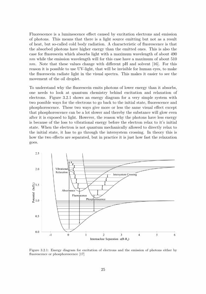
Fluorescence is a luminescence effect caused by excitation electrons and emissionof photons. This means that there is a light source emitting but not as a resultof heat, but so-called cold body radiation. A characteristic of fluorescence is thatthe absorbed photons have higher energy than the emitted ones. This is also thecase for fluorescein which absorbs light with a maximum wavelength of about 490nm while the emission wavelength will for this case have a maximum of about 510nm. Note that these values change with different pH and solvent [16]. For thisreason it is possible to use UV-light, that will be invisible for human eyes, to makethe fluorescein radiate light in the visual spectra. This makes it easier to see themovement of the oil droplet.

To understand why the fluorescein emits photons of lower energy than it absorbs,one needs to look at quantum chemistry behind excitation and relaxation ofelectrons. Figure 3.2.1 shows an energy diagram for a very simple system withtwo possible ways for the electrons to go back to the initial state, fluorescence andphosphorescence. These two ways give more or less the same visual effect exceptthat phosphorescence can be a lot slower and thereby the substance will glow evenafter it is exposed to light. However, the reason why the photons have less energyis because of the loss to vibrational energy before the electron relax to it’s initialstate. When the electron is not quantum mechanically allowed to directly relax tothe initial state, it has to go through the intersystem crossing. In theory this ishow the two effects are separated, but in practice it is just how fast the relaxationgoes.

Figure 3.2.1: Energy diagram for excitation of electrons and the emission of photons either byfluorescence or phosphorescence [17]

25

3.3 Filling and measure the capillary tubes

The apparatus itself is rather simple, capillary tubes. However the way they arefilled with different phases is more complicated. Figure 2.1.1 shows a sketch of thetube including the different phases. The challenge for this set up is to get all thephases into the capillary tube without having air bubbles. The air bubbles cancome at the interfacial regions and then a change in the interfacial contact, or thebubbles can come in the water phases and block the diffusion of water and sodiumchloride that needs to be there to keep a homogenous concentration.

The tubes were first filled by simply lowering them into the different solution incorrect order, and controlling the amount of liquid that get in by covering theother end of the tube. The capillary force was not strong enough to fill the tubecompletely, so the last water phase was injected with a syringe. This means thetube was lowered into solutions in the following order: water bulk phase (just alittle), oil phase, high salinity water phase, oil phase and water bulk phase again.The volume for each of the phases were controlled by how deep the tube werelowered. The end of the tube was turned and a syringe was moved into the smallwater bulk phase. By taking the syringe slowly out at the same time as releasingsome water made it possible to avoid air bubbles.

The tubs were put into the glass vessel in the water bath. The whole processwas done in two batches and it was always made three tubes with the samespecifications, so that the results could be compared with each other and alsoin case something went wrong. Except for the very smallest tube in the first batch.Here two of the glass tubes had incorrect phase layers, one with three oil dropletsand one with only a single. This was hard to visually observe when they weremade, but a look in the microscope discovered it. The two tubes where removed.

3.4 Accuracy and uncertainty

All the measurements were done by looking at the tubes in a microscope anddetermining the change in position relative to a marker line. A ruler was putbeside the tube as the reference. It is obvious that the uncertainty is rather highin the measurements where there are almost no change in position. However, it isvery hard to determine a specific uncertainty for all the measurements. The resultsfor volume flow and water flux are based on the average movement of the dropletover three measurements and the uncertainty is set to be the standard deviationof the three measurements. This excludes the uncertainty of the measurements,but the difference in the measurements are so high that it is covering all the otheruncertainties.

The uncertainty in the radius is varying form 0,5 to 0,6% of the volume of the tube.Least mean-square method are used for estimating the uncertainty of the radiusbased on this.

26

4 Observations

During the experiments different problems have been popping up, and the firstwas caused by various methods of filling the tubes. The injection worked well forthe largest tubes, but the syringe was too big for the smaller ones. The capillaryforce have been of great help, but it was not enough to fill the tubes. Most of thetimes there was a little room left in the tube. Also it was observed that it wasparticularly difficult to get the second oil phase into the tube, if the tube was filleda little too much it was impossible with the use of the capillary force, which wasthe only possibility found.

For the small tubes it was only one option, to fill them as much as possible andput them into the solution and then break them. Two tweezers were used to breakthe tubes. This gave a better and more precise breaking point rather than usinghands. The problem with breaking the tube is that the droplets usually moves alittle bit in the breaking process, and after they are put into the water bath it isnot possible to make any lines on the tube with a marker. However, by looking inthe microscope and measure the movement, one can compensate for the error.

The fluorescein effect was smaller than expected, and thereby not a big success. Itwas visible in the small tubes, but it requires very dark environment. Unfortunatelymy laboratory had large windows and the process of moving the tubes into adifferent room, together with the microscope, was not very good solution.

The accuracy of the measurements can always be questioned when the movementsare so small. It was also the case for this project. All measurements were done justby looking at the tubes in a microscope together with a ruler. I am sure this canbe further improved with a digital optical light microscope that can take pictures.Comparing the pictures from each measurement, can hopefully give better results.For the tubes with small movements it was crucial to know where on the markerline the measurements where done. A line with a normal thin marker would havea width of about 0, 2 − 0, 4mm, depending on if it is straight or not, and that ismore than the movement of the droplet.

Another factor that influence the accuracy is the formation of gas bubbles in thetube. The tubes in the first batch was filled with room tempered octane andwater solutions. This caused a problem because they were heated to 60oC andthereby a big change in vapor pressure that lead to formation of small bubbles. Aslong as the bubbles do not block the whole tube, there should be no problem forthe movement. But the bubbles will make the droplet larger. This will effect themovement depending on which direction the droplet expand. Luckily in this projectit was measured both sides of the droplet so it was possible to take into account thechange in size when measuring the movement, but I chose not to change thicknessof the droplet, δi, when calculating the fluxes.

27

5 Results

All the measurements that have been done are included in Appendix B, whilethe tabulated data for the calculations are in Appendix C. This includes all theexperimental data that have been used for the plots in this section. The resultspresented will be commented here, and further discussed in the next section. Avery important result of this project is the water flux equation already presentedin the theory.

Ja = −L 1T

[RT ln

(P2,vap

P1,vap

)+ 2Vo

(γw,h cos(θh)

rh− γw,l cos(θl)

rl

)]1δb

This clearly shows all the known forces contributing to the migration of water inthe capillary tubes. All the variables are in principle measurable, but the interfacialtension as a function of salt concentration is expensive and difficult to measure.

5.1 Chemical potential

The chemical potential differences over the droplets were calculated from thedifferences in vapor pressure according to Equation 2.2.3, and are presented inTable 5.1.1.

Table 5.1.1: Tabulated values of the difference in chemical potential for various sodium chlorideconcentrations against a 0,01M solution, at 60oC

c2 to c2 Pvap,2 Pvap for 0,01M ∆µ[mol/L] [kPa] [kPa] [kJ/mol]

5,0 to 0,01 11,13 19,96 1,622,5 to 0,01 15,12 19,96 0,771,0 to 0,01 17,91 19,96 0,300,5 to 0,01 18,90 19,96 0,15

5.2 Capillary force

The contribution from the capillary force can be estimated from equation 2.4.7.The problem is that there are many unknown variables in this equation. Theinterfacial tension is not known for the different sodium chloride concentrations,and neither is the contact angle. The radius of the meniscus will be the same as thetube radius if the contact angle is 0, and later is very often assumed for pure wateragainst glass. The change in interfacial tension for pure water have previously beendiscussed and the change is rather large at high salt concentrations. Figure 5.2.1shows a plot of the capillary force as a function of the radius of the meniscus withthe following conditions and assumptions:

• 25oC and 1 bar

28

• The contact angles are the same for both solutions

• The change in interfacial tension is set to be 5 mN/m (like it is for pure wateragainst 2,7M)

• The radius can be assumed to be the same as the tube radius

Figure 5.2.1: Simulated values for the capillary force as a function of the radius of the meniscusin the system under the conditions mentioned in the text.

As expected there is a large raise in the capillary force when the radius is gettingsmaller. The values are very well comparable to the one for the osmotic force,and for the small radiuses it is clear that the capillary force can influence. Theassumptions and conditions are very realistic as well.

5.3 Movement of the oil droplet

The measurements that have been taken clearly tell us that there is a movementof the oil droplets in the systems, and it is because of the osmotic gradient. Bychanging the concentrations of the sodium chloride solutions it is clear that iteffects the speed of the droplet. Figure 5.3.1 shows a plot of the water flux (overarea A) against the difference in chemical potential. Note that the capillary forceis not included in the chemical potential term, because it is not known for thedifferent solutions. If the capillary force has a significant impact on the system itwill contribute to the slope of the curve of this plot.

29

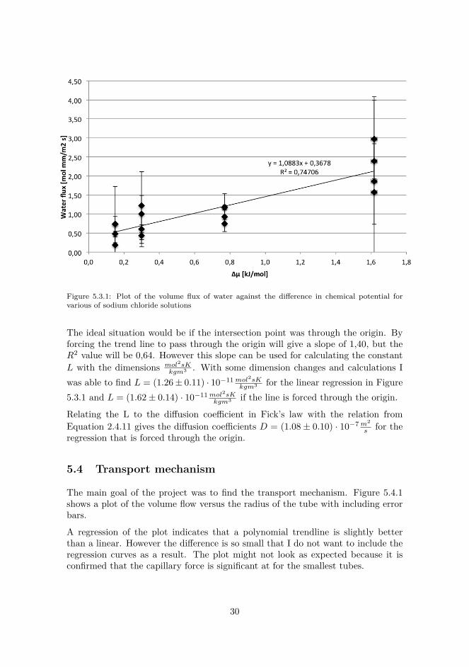
Figure 5.3.1: Plot of the volume flux of water against the difference in chemical potential forvarious of sodium chloride solutions

The ideal situation would be if the intersection point was through the origin. Byforcing the trend line to pass through the origin will give a slope of 1,40, but theR2 value will be 0,64. However this slope can be used for calculating the constantL with the dimensions mol2sK

kgm3 . With some dimension changes and calculations Iwas able to find L = (1.26± 0.11) · 10−11mol2sK

kgm3 for the linear regression in Figure5.3.1 and L = (1.62± 0.14) · 10−11mol2sK

kgm3 if the line is forced through the origin.

Relating the L to the diffusion coefficient in Fick’s law with the relation fromEquation 2.4.11 gives the diffusion coefficients D = (1.08 ± 0.10) · 10−7m2

s for theregression that is forced through the origin.

5.4 Transport mechanism

The main goal of the project was to find the transport mechanism. Figure 5.4.1shows a plot of the volume flow versus the radius of the tube with including errorbars.

A regression of the plot indicates that a polynomial trendline is slightly betterthan a linear. However the difference is so small that I do not want to include theregression curves as a result. The plot might not look as expected because it isconfirmed that the capillary force is significant at for the smallest tubes.

30

Figure 5.4.1: Plot of volume flow versus the radius for the system including error bars.

5.5 Distinguishing the two forces

To two contributing forces for the movement of the droplet are osmotic gradientand capillary force. From the experiments done it is unfortunately impossible todistinguish these two forces directly. However, as mention in the theory it can bedone with some assumptions. A plot of the water flow against the radius of thetube should give a straight line with a slope equal 0 if the capillary force does notcontribute. When or if the capillary force is large enough the line will change, mostlikely when the radius of the tube gets very small. Figure 5.2.1 shows the expectedsituation for simulated data. Figure 5.5.1 is the plot of the experimental values forthis project.

This plot shows a similar behavior as the one for the calculated values, but theincrease seems to come at even lower radiuses. This can very well be true, becausethe calculated data are based on some assumptions. It is good that the two plotshave similarities, and with more experiments it could be possible to give estimatesfor the change in interfacial tension and contact angle, which again will decide theradius of the meniscus. A plot of the theoretical total force, the capillary force andthe osmotic force together, against the radius is shown in Figure 5.5.2. This to givea better comparison to the experimental plot where both forces are included.

31

Figure 5.5.1: Plot of the water flow against the radius of the tube for the experiments

Figure 5.5.2: Plot of the total estimated force against the radius of the meniscus, with theassumptions mention earlier.

32

6 Discussion

This project has had many ups and downs and it is quite hard to find good solutionsfor all the problems. There were three main questions to start out with, and I havetried to answer them as good as possible. Sometimes it is not necessarily the resultthat makes the project good, but the knowledge of the mistakes and how to improvethe results. This is very important, and at least if one look at the accuracy of themeasurements done. At first it almost looked like a cloud of points, impossible tomake any regression or understand in any way, but that was of course and luckily,before I put in the correct formulas in excel.

6.1 Theoretical estimates

The two forces were theoretically calculated and the results were presented. Theosmotic force was calculated based on values for osmotic coefficient found byGibbard et al. [9], and are not really theoretically calculated, because they arebased on experiments. However, they are based on the assumption that the changein activity is equal the ratio of the vapor pressure, which is a pretty commonassumption. These values are for sure realistic and also used in the plots of theexperimental data.

The estimation of the capillary force is a little more vague. The conditions wereexplained in the results and I would like to verify them here.

- The first assumption is the temperature, which is 25 degrees celsius. It is knownthat the capillary force is lower at higher temperatures, so the values can beadjusted a little if one was to compare it directly with the experiments.

- The second assumption that the contact angle is the same for both sodium chlorideconcentrations is of course not completely true. The value of cosine to an angleclose to 0 does not change very much. From 0 to 10 degrees it changes from 1 to0.985, which is nothing compared to a small change in some of the other variables.Knowing that pure water has a contact angle of 0, makes this assumption quitereasonable.

- The third assumption was that the change in interfacial potential is about 5mN/mol is maybe the most questionable one. The change in interfacial tensionof pure water to a 2,7M water solution is about 5 mN/mol [13] and the change islinear with the concentration up to this value. If the trend continues over 2,7M, achange from 0,01M to 5,0M should give raise to an even larger change in surfacetension. However, I do not know if the change can apply for the interfacial tension.But looking at the estimates from Fawkes equation 2.3.3 one can see that theinterfacial tension seems to relate to the special interacting forces and not thedispersion forces. The special interacting forces for water are hydrogen bondings,which are highly polar bonds that the sodium chloride ions will interact with. Thensince the surface tension of water increases with salt concentration it is likely to

33

think that the interfacial tension does the same. I have chosen to only increase itwith 5 mN/mol, because I do not know weather the trend continues or not, so thisshould be on the safe side and cover for the assumptions. A larger change will ofcourse lead to an even larger effect from the capillary force, but it will not changethe shape of the curve and thereby not the point where it starts to increase faster.

- The fourth is not really an assumption, but it just makes it easier to comparewith the results if the statement is true. It also correlates with the assumptionthat the contact angle is close to zero.

The result of the plot is very interesting and it shows that the capillary force isexpected to contribute significantly at a radius lower than 0,2 mm. Although thereare some uncertainties involved, it still gives a quite realistic value as a start outpoint. The smallest tube used in the experimental part of this project is 0,15 mm,so one should expect the water flux of these tubes to be a littler higher.

6.2 Does the osmotic gradient effect the oil movement?

It is evident that the chemical potential difference is the reason for the movementof the oil droplet. The plot in Figure 5.3.1 has a quite good linear regression fit,with a slope that can correspond to the phenomenological coefficient, L. From theresults it does not look like the capillary force has any significant impact of thewater migration for the larges tubes, which are used for this plot. This is importantto know because the capillary force was not part of the variables in the plot andtherefor it would be participating in the slope of the curve.

There is one mysterious part of this plot, and that is the intersection point.Mathematically this means that there will be movements of the oil droplets evenwithout any concentration differences. However, I cannot see any other forces thatwould contribute to the movement, and it might just be my eager to see a changewhen I measured the movements. After all the movements were very close to zero,and it is difficult to measure the changes very accurate. A change on 1 mm couldgive quite a big impact on the results. This is something that very well can beimproved by letting the tubes stay longer or increase the temperature of the waterbath. The first option will for sure give longer distances, while the second is notcompletely sure.

The diffusion coefficient was reported, and it is reasonable compared with whatSchatzberg reported [18]. They reported diffusion coefficient to be 5, 97 · 10−5 cm2

sfor 45oC for n-hexadacane, which is about 20 times smaller than the reported resultin this report (note the difference in dimensions). If the results from Schatzbergare extrapolated to 60oC assuming a linear trend (R2 value of 0,99), it will give9, 03 · 10−5 cm2

s , and is only about 10 times smaller. It is likely to think that thesmaller octane molecules can transport water molecules faster and thereby havea higher diffusion coefficient. Water has also a higher solubility in octane than

34

hexadacane. This makes the result trustworthy and diffusion can be a very realistictransport mechanism for the water.

6.3 What is the mechanism for the water migration?

This was set as the main question for the whole project, and the results are yet notvery clear. The experiments are very narrow and only look at completely circulartubes made of glass. It will be very different in a real oil reservoir where the wallsare made of porous stone and not at all circular. If the walls are more hydrophobicmaybe it will favor a bulk diffusion. On the other side, if the walls have variousshapes and are hydrophilic it will for sure favor migration along the walls but willit open for transfer of sodium chloride ions as well? Figure 6.3.1 shows the crosssection of two possible pore shapes, not suppose to illustrate real situation, butjust as examples. A system always wants to be in the lowest energy state, and ifthe oil is not attracted to the walls it will want to form spheres to reduce the totalsurface tension. That is why it will not fill all the corners on the sketch. This shapewill leave cavities for the water to migrate, and if they are big enough it would bepossible to transport ions as well.

Figure 6.3.1: Example of the cross section of two possible pore shapes

The results of this project are difficult to draw any conclusion from. It is only threedifferent radiuses and two of them are too close to each other. It would have beendesirable to have more variation in size and more measurements, but this was theequipment given and I actually thought it would be enough. However, during a 4months project it is hard to know what the outcome will be, when each experimenttakes about 40 days. It would defiantly have been interesting to have a point in-between the radius of 0,23 and 0,70, and maybe a point larger than 0,70. Thiscould perhaps have been sufficient for drawing a conclusion, but the inaccuracywould still have been a big problem.

A linear regression gives a R2 value of 0,86 while a second degree polynomialregression gives 0,88. However, by looking at the curve it seems like the polynomialfits better for the low values. This might be because one of the points for the smallerradius is very high, and a polynomial fit allows the trendline to have a minimumand then increase again. Removing this point does not help either. Then both the

35

regressions have 0,88 in R2 value. One also needs to keep in mind that the pointsfor the smallest radius in reality are not relevant because the capillary force willcontribute and change the shape of the curve.

6.4 Will the capillary force contribute?

The theoretical estimations tells us that the capillary force should contribute forthe smallest tubes size. From the plot in Figure 5.5.1 one can see that the water fluxincreases slightly for the smallest tube and thereby it verifies the estimations done.The size of the increase is not possible to say something about. However, theseresults have some assumptions and there are only two points from the smallesttube and both with quite high uncertainty. One of the points seems to be wayhigher than expected and might not be very reliable, and one point is not much todraw conclusions from for these experiments. I have previously discussed how highthe uncertainty of the measurements can be, however it decreases with increasingconcentration difference. But this is only the uncertainty related to the actuallymeasurements. However, all the fluxes are based on the average flux over threemeasurements, and the standard deviation of the average (the one used in theplots) is in many cases as high as the numerical value for the water flux. I wouldnot have counted my life on these results, but they indicates that the capillaryforce can very well contribute.

A very good way to improve the results for this experiments will be first of all tochange the walls of the capillary tube and see the effect on the speed. This can,as mentioned earlier, change the transport mechanism because water will attractmore/less to the walls. That is why another solution might be even better. This isto plot the water flux against the differences in chemical potential like Figure 5.3.1,and for various of tube sizes. Then compare the slope of the curves, meaning the Lvalue, for the different plots. If the L is dependent on the radius of the tube, thenit will be clear that the capillary force contributes, if not the opposite of course.If the measurements are done for a large variety of tube sizes one can plot the Lagainst the radius and see at witch radius the capillary force starts to contributesignificantly. The plot will hopefully give a straight line for the large radiuses andthen starts to change when the radius is getting lower.

36

7 Conclusion

The transport mechanism of water from one side of the oil droplet to the other, wasthe first problem to solve in this project. The experimental diffusion coefficient isin the same order of magnitude as expected for bulk diffusion coefficient. However,no such estimations were possible to do for the surface diffusion, so it can very wellfit for this transport mechanism as well. The conclusion is that the water migratesbecause of the concentration difference of sodium chloride, and the experimentscan confirm that a bulk diffusion can be the mechanism, but one cannot excludethe possibility of a surface diffusion along the walls.

The capillary force was estimated with some assumptions, and the experimentalresults confirmed a similar trend. It seems like the capillary force starts tosignificantly contribute to the water migration, when the radius of the tube issmaller than 0,20 mm. This means that if the tube radius is larger than 0,20 mm,then the movement is controlled by the difference in chemical potential.

37

8 Nomenclature

Symbol Dimension Descriptionai − Activity of component i in solutionA m2 Area (of the flux)c mol/L Concentrationδ m Width of the oil dropletδr m Difference in radiusJi mol/m2s Molar flux of component iJv m3/m2s Volume flux of waterFc N Capillary forceG J/mol Gibbs’ energyGoi J/mol Gibbs’ standard energy for component iΓi mol/m2 Surface excess for component iγi mN/m Surface tension for component iγdisp mN/m Surface tension caused by dispersion forcesγsp mN/m Surface tension caused by spacial interactionsλi − Activity coefficient for component iLij − Phenomenological coefficientm mol/kg Molalityµi J/mol Chemical potential for component iµoi J/mol Chemical potential for a pure component ini mol Amount of substance iO m Three phase contact linePi Pa PressureP oi Pa Pressure for reference conditionsPvap Pa Vaporization pressureR J/molK Universial gas constantr m Radius of he meniscusρ g/mL DensitySirr J/Kmol Irreverisble entropy productionσi J/Kmolm Local entropy productionT K Temperaturet day Timeθ o Contact angleVi L/mol Molarity for the pure component iV L/s Volume flowvw m/day Speed of the dropletxi − Mol fraction∆x m Change in position of the oil droplet

38

References

[1] E. Tzimas, A. Georgakaki, C. Garcia Cortes, and S. D. Peteves. Enhancedoil recovery using carbon dioxide in the european energy system. DG JRCInstitute for Energy, Petten, The netherlands, 2005.

[2] U.S. Department of Energy. Enhanced oil recovery/co2 injection.http://www.fossil.energy.gov/programs/oilgas/eor/index.html.

[3] L. Wen and K. D. Papadopoulos. Effect of osmotic pressure on water transportin w1/o/w2 emulsions. Journal of Colloid and Interface Science, 235:398–404,2001.

[4] J. Cheng, J.-F. Chen, M. Zhao, Q. Luo, L.-X. Wen, and K. D. Papadopoulos.Transport of ions through the oil phase of w1/o/w2 double emulsions. Journalof Colloid and Interface Science, 305:175–182, 2007.

[5] Jon Brandsar and Aslak Øverås. Crown princess of norway to open the world’sfirst osmotic power plant @ONLINE, http://www.statkraft.com/presscenter/,October 2009.

[6] X. Zhou, N. R. Morrow, and S. Ma. Interrelationship of wettability, initialwater saturation, aging time, and oil recovery by spontaneous imbibition andwaterflooding. SPE Journal, 5:199–207, 2000.

[7] P. Atkins and J. Paula. Physical Chemistry. W. H Freeman and Company2010, New York-, 2010.

[8] G. Scatchard, W. J. Hammer, and S. E. Wood. Isotonic solutions. i. thechemical potential of water in aqueous solutions of sodium chloride, potassiumchloride, sulfuric acid, sucrose, urea and glycerol at 25◦. Journal of theAmerican Chemical Society, 60:3061–3070, 1938.

[9] H. F. Gibbard Jr., G. Scatchard, R. A. Rousseau, and J. L. Creek. Liquid-vapor equilibrium of aqueous sodium chloride, from 298 to 373k and from 1to 6 mol kg−1, and related properties. Journal of Chemical and EngineeringData, 19:280–287, 1974.

[10] John A. Dean. Lange’s Handbook of Chemistry. McGraw-Hill Professional,11th edition, 1967.

[11] P.C Mørk. Overflate og Kolloidkjemi, Grunnleggende prinsipper og teorier.Department of chemical process technology, NTNU, 7th edition, 2001.

[12] J. Vanhanen, A.-P. Hyvarinen, H. Lihavainen, Y. Viisanen, and M. Kulmala.Surface tensions of sodium chloride/succinic acid/water solutions. EuropeanAerosol Conference 2007, 2007.

[13] A. Horibe, S. Fukusako, and M. Yamada. Surface tension of low-temperatureaqueous solutions. International Journal og Thermophysics, 17 No. 2:483–493,1996.

39

[14] H.-J. Butt, K. Graf, and M. Kappl. Physics and Chemistry of Interfaces.WILEY-VCH Verlag GmbH & Co. KGaA, Weinheim, 1st edition, 2006.

[15] Lars Onsager. Reciprocal relations in irreversible processes. i. Physical Review,37:405–426, 1931.

[16] R. Sjöback, J. Nygren, and M. Kubista. Absorption and fluorescence propertiesof fluorescein. Spectrochimica Acta, Part A 51:L7–L21, 1995.

[17] P. Atkins, J. de Paula, and R. Froedman. Quanta, Matter, and Change Amolecular approach to physical chemistry. W.H. Freeman, New York, 2009.

[18] Paul Schatzberg. Diffusion of water through hydrocarbon liquids. Journal ofpolymer science, 10:87–92, 1965.

40

A Calculations of vapor pressure of water at 60oC

The data found were the osmotic coefficients at different molalities at 60oC. Thisneeds to be calculated to vapor pressure for different molarities. First by findingthe relationship between molalities and molarities at 60oC [10]. The tabulated datais listed in Table A.0.1 and a plot can be seen in Figure A.0.1

Table A.0.1: Tabulated values of molality and density.m[mol/kg] ρ[g/mL]0,09842 0,98340,19683 0,98760,49160 1,00290,98320 1,02241,96300 1,05883,92200 1,1295

Figure A.0.1: Plot of density versus molality at 60oC

The regression gives the following relation, where ρ is the density in g/mL and mis the molality in mol/kg

ρ = 0, 038m+ 0, 9823 (A.0.1)

The molarity was calculated and can be found together with the osmotic coefficientsin Table A.0.2. The osmotic coefficient for 60oC was estimated by interpolationbetween the values for 50oC and 75oC. The vapor pressures were calculated fromthe estimated values and plotted against the concentration in Figure 2.2.1. Thetabulated values are given in Table A.0.3.

41

Table A.0.2: Tabulated values for osmotic coefficient for different temperatures and concentra-tions.m[mol/kgl] c[mol/L] T = 323, 15K T = 348, 15K Estimated T = 333, 15K

0,10 0,10 0,9317 0,9281 0,93030,20 0,20 0,9235 0,9198 0,92200,30 0,30 0,9214 0,9179 0,92000,40 0,40 0,9219 0,9185 0,92050,50 0,50 0,9237 0,9206 0,92250,60 0,60 0,9264 0,9236 0,92530,70 0,71 0,9297 0,9271 0,92870,80 0,81 0,9335 0,9311 0,93250,90 0,91 0,9376 0,9354 0,93671,00 1,02 0,9419 0,9399 0,94111,20 1,23 0,9513 0,9496 0,95061,40 1,45 0,9614 0,9598 0,96081,50 1,56 0,9666 0,9652 0,96601,60 1,67 0,9720 0,9706 0,97141,80 1,89 0,9831 0,9816 0,98252,00 2,12 0,9946 0,9930 0,99402,50 2,69 1,0249 1,0226 1,02403,00 3,29 1,0567 1,0533 1,05533,50 3,90 1,0898 1,0847 1,08784,00 4,54 1,1238 1,1166 1,12094,50 5,19 1,1583 1,1484 1,15435,00 5,86 1,1932 1,1800 1,18795,50 6,55 1,2282 1,2110 1,22136,00 7,26 1,2631 1,2410 1,2543

Table A.0.3: Tabulated values for vapor pressure for sodium chloride solutions at differentconcentrations, 60oC.

c[mol/L] Vapor pressure [kPa]0,10 19,70,20 19,50,30 19,30,40 19,10,50 18,90,60 18,70,71 18,50,81 18,30,92 18,11,02 17,91,23 17,51,45 17,01,56 16,81,67 16,61,89 16,22,12 15,82,69 14,83,29 13,83,90 12,84,54 11,85,19 10,95,86 9,956,55 9,097,26 8,27

42

B Measurements

The experiments were done in two different batches. For each of the batches therewas in total 18 capillary tubes, six different systems and three of each. For the firstbatch the movement of the droplet was measured after 18, 27 and 42 days, whilethe second was only measured after 13 days. All the measurements can be viewedin Table B.0.4.

Table B.0.4: Tabulated values of the movements for batch one and two.* measurement was doneafter 27 daysTube id ∆x in 18 days [mm] ∆x in 9 days [mm] ∆x in 15 days [mm] ∆x in 13 days [mm]5M #1 1,33 -0,15 0,48 -5M #2 0,90 0,20 0,65 -5M #3 1,05 0,15 0,45 -5M #4 - - - 0,305M #5 - - - 0,405M #6 - - - 0,302,5M #1 0,38 0,20 0,33 -2,5M #2 0,20 0,18 0,28 -2,5M #3 - 0,33 0,28 -2,5M #4 - - - 0,152,5M #5 - - - 0,102,5M #6 - - - 0,101,0M #1 0,53 0,08 0,15 -1,0M #2 0,28 0,03 0,15 -1,0M #3 0,15 0,13 0,05 -1,0M #4 - - - 0,101,0M #5 - - - 0,101,0M #6 - - - 0,150,5M #1 0,00 0,03 0,13 -0,5M #2 0,25 0,08 0,15 -0,5M #3 0,18 0,18 -0,05 -0,5M #4 - - - 0,100,5M #5 - - - 0,050,5M #6 - - - 0,155uL #1 2,30 0,83 3,435uL #2 - - - 1,055uL #3 - - - 0,555uL #4 - - - 0,6510uL #1 0,80 0,15 0,70 -10uL #2 1,30 1,05 0,93 -10uL #3 1,38 0,18 0,98 -10uL #4 - - - 0,2010uL #5 - - - 0,5010uL #6 - - - 0,60

The corresponding thicknesses of the droplets can be seen in Table B.0.5.

43

Table B.0.5: Tabulated values of the thicknesses of the droplets for all systems, together with theaverage

Tube id δ1, left droplet [mm] δ2, right droplet [mm] Average δ [mm]5M #1 2,8 1,5 2,25M #2 4,8 2,0 3,45M #3 1,9 2,0 2,05M #4 2,9 4,0 3,55M #5 4,6 2,8 3,75M #6 4,0 2,9 3,52,5M #1 2,0 2,0 2,02,5M #2 1,9 1,5 1,72,5M #3 2,2 4,1 3,22,5M #4 3,8 3,3 3,62,5M #5 3,0 4,6 3,82,5M #6 3,2 6,7 5,01,0M #1 3,1 2,6 2,91,0M #2 1,6 1,8 1,71,0M #3 2,4 2,8 2,61,0M #4 4,6 5,7 5,21,0M #5 4,0 1,6 2,81,0M #6 3,5 6,7 5,10,5M #1 1,8 1,9 1,90,5M #2 2,8 2,3 2,60,5M #3 3,8 2,7 3,30,5M #4 5,4 1,2 3,30,5M #5 5,5 1,8 3,70,5M #6 2,3 2,4 2,45uL #1 3,2 1,4 2,35uL #2 2,2 0,9 1,65uL #3 3,0 2,8 2,95uL #4 4,2 4,1 4,210uL #1 2,1 1,4 1,810uL #2 1,7 1,0 1,410uL #3 3,0 1,5 2,310uL #4 3,7 1,6 2,710uL #5 4,6 1,0 2,810uL #6 6,7 4,0 5,4

44

C Tabulated values for the calculations

The calculated water fluxes can be observed in Table C.0.6. Note that these valuesare volume flow per area and thereby dependent on the area of the tube.

Table C.0.6: Tabulated data for the water flux for the different measurements, all at 60oC. TheA is the cross sectional area of the tubes. *Average is taken over three measurements

Tube id First meas. Jw Second Jw Third Jw Avg. Jw STDEV[mol mm [mol mm [mol mm [mol mm [mol mmm−2day−1] m−2day−1] m−2day−1] m−2day−1] m−2day−1]

5M #1 3,9 -0,9 1,7 1,6 2,45M #2 3,8 1,7 3,3 3,0 1,15M #3 3,1 0,9 1,6 1,9 1,15M #4 2,1 - -5M #5 2,9 - - 2,4* 0,55M #6 2,1 - -2,5M #1 1,14 1,2 1,2 1,2 0,042,5M #2 0,5 0,9 0,8 0,7 0,22,5M #3 - 0,9 1,4 1,2 0,32,5M #4 1,11 - -2,5M #5 0,76 - - 0,93 * 0,182,5M #6 0,91 - -1,0M #1 2,3 0,6 0,8 1,2 0,91,0M #2 0,7 0,1 0,4 0,4 0,31,0M #3 0,6 1,0 0,2 0,6 0,41,0M #4 1,1 - -1,0M #5 0,5 - - 1,0* 0,51,0M #6 1,5 - -0,5M #1 0,0 0,1 0,4 0,2 0,20,5M #2 1,0 0,6 0,7 0,7 0,20,5M #3 0,8 1,7 -0,3 0,7 1,00,5M #4 0,4 - -0,5M #5 0,3 - - 0,5* 0,20,5M #6 0,7 - -5µL #1 6,8 15 12 11,4 4,35µL #2 2,8 - -5µL #3 3,4 - - 3,9* 1,55µL #4 5,7 - -10µL #1 2,0 0,8 2,1 1,6 0,810µL #2 2,5 4,0 2,1 2,9 1,010µL #3 4,2 1,1 3,5 2,9 1,610µL #4 0,9 - -10µL #5 1,7 - - 3,0* 2,910µL #6 6,3 - -

45

Table C.0.7 shows the calculated volume flow, in this case meaning the volume ofwater per day in total, not just over a specific area.

Table C.0.7: Tabulated data for the volume flow of water for the different measurements, all at60oC. *Average is taken over three measurements

Tube id Volum flow 1 Volum flow 1 Volum flow 1 Avg. volume flow STDEV[µLm/day] [µLm/day] [µLm/day] [µLm/day] [µLm/day]

5M #1 0,24 -0,06 0,10 0,10 0,155M #2 0,26 0,12 0,23 0,20 0,085M #3 0,18 0,05 0,09 0,11 0,065M #4 0,12 - -5M #5 0,18 - - 0,14* 0,035M #6 0,12 - -2,5M #1 0,06 0,07 0,07 0,066 0,0022,5M #2 0,03 0,05 0,05 0,043 0,0122,5M #3 - 0,06 0,09 0,07 0,022,5M #4 0,06 - -2,5M #5 0,04 - - 0,055* 0,0092,5M #6 0,06 - -1,0M #1 0,13 0,04 0,04 0,07 0,051,0M #2 0,04 0,01 0,03 0,025 0,0161,0M #3 0,03 0,06 0,01 0,03 0,021,0M #4 0,06 - -1,0M #5 0,03 - - 0,06* 0,031,0M #6 0,09 - -0,5M #1 0,00 0,01 0,02 0,011 0,0120,5M #2 0,05 0,03 0,04 0,042 0,0110,5M #3 0,05 0,10 -0,02 0,04 0,060,5M #4 0,04 - -0,5M #5 0,02 - - 0,034* 0,0110,5M #6 0,04 - -5µL #1 0,020 0,045 0,036 0,0337 0,0135µL #2 0,008 - -5µL #3 0,008 - - 0,010* 0,0035µL #4 0,014 - -10µL #1 0,013 0,005 0,014 0,010 0,00510µL #2 0,016 0,026 0,014 0,019 0,00710µL #3 0,029 0,007 0,024 0,020 0,01110µL #4 0,007 - -10µL #5 0,018 - - 0,022* 0,01810µL #6 0,041 - -

46