Capital Allocation and the Market for Mutual Funds:

Inspecting the Mechanism∗

Jules H. van Binsbergen Jeong Ho (John) Kim

University of Pennsylvania and NBER Emory University

Soohun Kim

Georgia Institute of Technology

October 1, 2019

Abstract

We analyze the effects of returns to scale on capital allocation decisions in the

mutual fund market by exploiting individual heterogeneity in decreasing returns to

scale across funds. We find strong evidence that steeper decreasing returns to scale

attenuate flow sensitivity to performance and lead to smaller fund sizes. Our results

are consistent with a rational model for active management. Using the model, we argue

that a large fraction of capital allocation due to differences in decreasing returns to

scale can be plausibly attributed to investors anticipating these effects of scale.

∗We thank seminar participants at Emory University for their comments and suggestions.

1 Introduction

An important question in financial economics is whether investors effi ciently allocate capital

across financial assets. Under the standard neoclassical assumptions, investors compete

with each other for positive present value opportunities, and by doing so, remove them in

equilibrium. In the case of mutual funds, the literature has argued that decreasing returns

to scale (DRS) play a key role in equilibrating the mutual fund market (Berk and Green

(2004)). Because the percentage fee that mutual funds charge changes infrequently, the bulk

of the equilibration process operates through the size (or Assets Under Management (AUM))

of the fund. When good news about a mutual fund arrives, rational Bayesian updating will

lead investors to view the fund as a positive Net Present Value (NPV) buying opportunity

at its current size. In response, flows will go to that fund. As the fund grows, the manager

of the fund finds it increasingly harder to put the new inflows to good use, leading to a

deterioration of the performance of the fund. The flows into the fund will stop when the

fund is no longer a positive NPV investment, and the fund’s abnormal return to investors

has reverted back to zero.

In this paper we investigate this equilibrating mechanism more closely. In particular,

if the above-mentioned equilibration process is at work, we should expect to find that the

degree of decreasing returns to scale (DRS) can have implications for the flow sensitivity to

performance (FSP). While there is much evidence that an active fund’s ability to outperform

its benchmark declines as its size increases,1 there is surprisingly little empirical work devoted

to whether investors account for the adverse effects of fund scale in making their capital

allocation decisions.

We address this important question by formally deriving and empirically testing what a

rational model for active management implies about the relation between returns to scale

and flow sensitivity to performance. Using a theory model similar to that of Berk and

Green (2004), we show that steeper decreasing returns to scale attenuates flow sensitivity

to performance. In the model, investors rationally interpret high performance as evidence

of the manager’s superior skill, so good performance results in an inflow of funds. More

importantly, the magnitude of the capital response is primarily driven by the extent of

decreasing returns to scale. As a fund’s returns decrease in scale more steeply, the positive

net alpha is competed away with a smaller amount of capital inflows, making flows less

sensitive to performance.

To test this theoretical insight, one needs a source of heterogeneity in decreasing re-

1See, for example, Chen et al. (2004), Yan (2008), Ferreira et al. (2013), and Zhu (2018).

1

turns to scale. One also needs to observe investor reactions to this heterogeneity. Indeed,

we demonstrate that there is a substantial amount of heterogeneity in DRS across individ-

ual funds, with correspondingly heterogeneous flow sensitivity to performance across funds.

Our approach can be interpreted as inferring how the subjective size-performance relation,

perceived by investors in real time, is incorporated into the flow-performance relation go-

ing forward. We find that a steeper decreasing returns to scale parameter predicts a lower

sensitivity of flows to performance, consistent with the main prediction of our model.

One of the challenges in estimating the effect of decreasing returns to scale on flow

sensitivity to performance is the estimation error in fund-specific DRS. As a result, the point

estimates of the DRS-FSP relation using DRS estimates from simple fund-by-fund regressions

are likely to suffer from an errors-in-variables bias. We alleviate the errors-in-variables bias

by relating the heterogeneity in decreasing returns to scale to a set of fund characteristics. In

particular, by regressing the fund-specific DRS estimates on these characteristics, we obtain

fitted values that we use as a more robust way of obtaining cross-sectional variation. We find

the degree of DRS is stronger for higher-volatility funds, sole-managed funds, older funds, as

well as funds that have experienced outflows in the past year. Next, we show that while the

statistical significance of the DRS-FSP relation is unaffected by using characteristic-based

DRS, the point estimates become substantially more negative, suggesting that the projection

onto characteristics indeed has alleviated the errors-in-variables problem.

Next we turn to the economic significance of our estimates. In particular, we assess how

equilibrium fund size is affected by the cross-sectional variation in decreasing returns to scale

parameters. This exercise does require model assumptions. We calibrate a rational model

in the spirit of Berk and Green (2004) to compute counterfactual fund sizes. We find that

at least 49% of the cross-sectional variance of fund sizes can be related to cross-sectional

variation in decreasing returns to scale parameters. More importantly, the uncalibrated

version of our model with heterogeneous returns to scale can quantitatively reproduce capital

allocation in the version calibrated to the empirical DRS-FSP relationship. We also find

that the DRS-FSP relation estimates in the uncalibrated version tend to be substantially

more negative than those from the data. Thus, it appears that investors in the data face a

substantially harder learning problem than in our simple model, though we leave identifying

additional aspects of learning to explain this gap as a question to be explored by future

research.

Beyond implications for fund flows, steeper decreasing returns to scale has implications

for fund size in equilibrium. In the model, fund size in equilibrium is proportional to the

ratio of perceived skill over diseconomies of scale, which predicts that, all else equal, the

2

decreasing returns to scale parameter should be lower for larger funds. This prediction is

confirmed in our empirical analysis. Moreover, if investors update their beliefs about skill

as in the model, their perception of optimal size ought to converge to true optimal size as

funds grow older. Consistent with this argument, we find that estimates for the optimal size

largely explains capital allocation across older funds in the data. We measure (log) optimal

size by the average ratio of the usual net alpha that is adjusted for returns to scale over

the characteristic-based DRS. We show that older fund’s size continues to be significantly

related to our measure of its optimal size even when we control for an alternative measure

of optimal size that assumes fund scale has the same effect on performance for all funds.

Again, investors seem to account not only for the presence of decreasing returns to scale,

but also for the heterogeneity of decreasing returns to scale across funds.

Taken together, our results demonstrate that investors do account for the adverse effects

of fund scale in making their capital allocation decisions, and that the rational expectations

equilibrium does a reasonable job of approximating the observed equilibrium in the mutual

fund market. In contrast, mutual fund investors were generally deemed naive return chasers

because fund flows respond to past performance even though performance is not persistent.2

Furthermore, many papers in the mutual fund literature have documented that mutual fund

returns show little evidence of outperformance.3 While these findings led many researchers

to question the rationality of mutual fund investors, Berk and Green (2004) argue that they

are consistent with a model of how competition between rational investors determines the

net alpha in equilibrium. We contribute to this debate by presenting findings that are hard

to reconcile with anything other than the existence of rational fund flows.

2 Definitions and hypotheses

To formally derive our hypothesis, we use the notation and setup presented in Berk and

van Binsbergen (2016). Let qit denote assets under management (AUM) of fund i at time

t and let θi denote a parameter that describes the skill of the manager of fund i. At time

t, investors use the time t information set It to update their beliefs on θi resulting in the

distribution function gt (θi) implying that the expectation of θi at time t is: Z θit ≡ E [θi |It ] = θigt (θi) dθi. (1)

2See Chevalier and Ellison (1997) and Sirri and Tufano (1998), among others. 3See Jensen (1968), Malkiel (1995), Gruber (1996), Fama and French (2010), and Del Guercio and Reuter

(2013), among others.

3

We assume throughout that gt (·) is not a degenerate distribution function. Let Rnit denote

the return in excess of the risk free rate earned by investors in fund i at time t. This return

can be split up into the excess return of the manager’s benchmark, RitB , and a deviation from

the benchmark εit:

Rnit = RBit + εit. (2)

Note that qit, Rn and RB are elements of It. Let αit (q) denote investors’subjective expec-it it

tation of εi,t+1 when investing in fund i that has size q between time t and t + 1, and let it

be equal to:

αit (q) = θit − hi (q) , (3)

where hi (q) is a strictly increasing function of q that captures the decreasing returns to scale

the manager faces, which can vary by fund. In equilibrium, the size of the fund qit adjusts to

ensure that there are no positive net present value investment opportunities so αit (qit) = 0

and

θit = hi (qit) . (4)

At time t + 1, the investor observes the manager’s return outperformance, εit+1, which is a

signal that is informative about θi. The conditional distribution function of εi,t+1 at time t,

ft (εit+1), satisfies the following condition in equilibrium: Z E [εit+1 |It ] = εit+1ft (εit+1) dεit+1 = αit (qit) = 0. (5)

In other words, the manager’s return outperformance can be expressed as follows:

εit+1 = θi − hi (qit) + �it+1

= sit+1 − hi (qit) ,

where sit+1 = θi +�it+1. Our hypothesis relies on the insight that good news, that is, high sit,

implies good news about θi and bad news, low sit, implies bad news about θi. The following

lemma shows that this condition holds generally. That is, θit is a strictly increasing function

of sit.

Lemma 1 If the likelihood ratio ft (sit+1 |θi ) /ft (sit+1 |θci ) is monotone in sit+1, increasing

if θi > θci and decreasing otherwise,

∂θit+1 > 0. (6)

∂sit+1

Proof. See Milgrom (1981).

4

In addition, we assume that the costs that manager i faces in expanding the fund’s scale

is given by:

hi (q) = bih (q) , (7)

where bi > 0 is a parameter that captures the cross sectional variation in the fund’s returns to

scale technology and h (q) is a strictly increasing function of q, which essentially determines

the form of decreasing returns to scale technology that is common across all funds. Using

(7) to rewrite (4) now gives � � θit

qit = h−1 . (8) bi

The following lemma shows how the size of the fund qit depends on the information in sit or

the parameter bi.

Lemma 2 ∂qit 1 ∂θit

= (9) ∂sit bih0 (qit) ∂sit

and ∂qit h (qit)

= − . (10) ∂bi bih0 (qit)

Proof. First, note that εit does not contain information about managerial ability that is

not already contained in sit. Because rescaling the fund’s returns to scale technology (i.e.,

changing the parameter bi) does not change the signal sit, we can conclude that

∂θit = 0. (11)

∂bi

Now differentiating (8) with respect to sit, and using the fact that these signals are inde-

pendent of bi (i.e., ∂bi/∂sit = 0), gives � � ∂qit 1 ∂ θit/bi 1 ∂θit 1 ∂θit

= � � = � � = ,∂sit h0 θit/bi ∂sit bih0 θit/bi ∂sit bih0 (qit) ∂sit

where the last equality follows from (8). Similarly, differentiate (8) with respect to bi, and

use (11) to substitute for ∂θit/∂bi in this expression. Appealing, again, to (8), gives (10).

Next, let the flow of capital into mutual fund i at time t be denoted by Fit, that is,

Fit+1 ≡ log (qit+1/qit) .

5

Differentiating this expression with respect to sit+1,

∂Fit+1 1 dqit+1 1 1 ∂θit+1 = = > 0,

∂sit+1 qit+1 dsit+1 qit+1 bih0 (qit+1) ∂sit+1

where the second equality follows from (9) and the inequality follows from Lemma 1, so good

(bad) performance results in an inflow (outflow) of funds. This result is one of the important

insights from Berk and Green (2004).

Given the importance of returns to scale technology in determining the size of a fund, a

natural question to ask is, what is the implication of steeper decreasing returns to scale for

the flow-performance relation? We answer this question by computing the derivative of the

flow-performance sensitivity with respect to bi: � � � � ∂ ∂Fit+1 ∂ 1 1 ∂θit+1

= ∂bi ∂sit+1 ∂bi qit+1 bih0 (qit+1) ∂sit+1

∂qit+1qit+1h0 (qit+1) + (bih

0 (qit+1) + qit+1bih00 (qit+1))∂bi ∂θit+1 = − 22qit+1 (bih

0 (qit+1)) ∂sit+1� � qit+1h

0 (qit+1) − h (qit+1) 1 + qit+1h00(qit+1)

h0(qit+1) ∂θit+1 = − 2 , (12)

q2 ∂sit+1it+1 (bih0 (qit+1))

where the first equality follows from (11) because when θit+1 is solely a function of the history � � ∂ ∂θit+1of realized signals and is not a function of bi then = 0 and the last equality follows ∂bi ∂sit+1

from (10). What (12) combined with Lemma 1 tells us is that steeper decreasing returns to

scale must lead to a smaller flow of funds response to performance if and only if � � qit+1h

00 (qit+1) qit+1h

0 (qit+1) − h (qit+1) 1 + > 0. (13) h0 (qit+1)

Unfortunately, the left hand side of Equation 13 is not easy to sign without further assump-

tions. To assess whether this condition holds, we rely on the second-order approximation to

the decreasing returns to scale technology:

h (q) ' h0 + h1 log (q) + h2 log (q)2 , (14)

where hi for i = {0, 1, 2} are the coeffi cients in the second-order approximation. This approx-

imation nests exactly specifying the technology as logarithmic, most commonly considered

in empirical studies, if we set h1 > 0 and h0 = h2 = 0. Going forward, we set h0 = 0.

This assumption is without loss of generality, because we can rewrite the skill parameter as

6

θ0 i = θi − bih0, which, in turn, renders h0 0 = 0. The following proposition shows that, under

approximation (14), condition (13) holds generally. That is, steeper decreasing returns to

scale leads to a weaker flow response to performance. We take this as our main hypothesis

that we will take to the data.

Proposition 3 Under approximation (14), the derivative of the flow-performance sensitivity

with respect to the decreasing returns to scale parameter is negative, that is, � � ∂ ∂Fit+1

< 0. ∂bi ∂sit+1

Proof. Under approximation (14), the left-hand side of (13) is then given by: !2h2−(h1+2h2 log(qit+1))� 2� qit+1h1 + 2h2 log (qit+1) − h1 log (qit+1) + h2 log (qit+1) 1 + h1+2h2 log(qit+1)

qit+1 � 2� 2h2 = h1 + 2h2 log (qit+1) − h1 log (qit+1) + h2 log (qit+1)

h1 + 2h2 log (qit+1)� � (h1 + 2h2 log (qit+1))

2 − 2 h1 log (qit+1) + h2 log (qit+1)2 h2

= h1 + 2h2 log (qit+1)

(h1 + h2 log (qit+1))2 + h22 log (qit+1)

2

= . h1 + 2h2 log (qit+1)

The numerator of this expression is the sum of two squares, so it is positive. Note that the

denominator can be rewritten as the product of qit+1 and h0 (qit+1) under the given approx-

imation. Recall that h (q) is a strictly increasing function of q, reflecting the fact that all

mutual funds must face decreasing returns to scale in equilibrium. Requiring that, under the

approximation, h0 (qit+1) > 0 is also ensured, this means that the denominator is positive as

well. It then follows immediately that condition (13) holds, which completes the proof.

3 Data

Our data come from CRSP and Morningstar. We require that funds appear in both CRSP

and Morningstar, which allows us to validate data accuracy across the two databases. We

merge CRSP and Morningstar based on funds’tickers, CUSIPs, and names. We then com-

pare assets and returns across the two sources in an effort to check the accuracy of each

match following Berk and van Binsbergen (2015). We refer the readers to the data appen-

dices of that paper for the details. Our mutual fund data set contains 3,066 actively managed

domestic equity-only mutual funds in the United States between 1979 and 2014.

7

We use Morningstar Category to categorize funds into nine groups corresponding to

Morningstar’s 3×3 stylebox (large value, mid-cap growth, etc.). We also use keywords in the

Primary Prospectus Benchmark variable in Morningstar to exclude bond funds, international

funds, target funds, real estate funds, sector funds, and other non-equity funds. We drop

funds identified by CRSP or Morningstar as index funds, in addition to funds whose name

contains “index.”We also drop any fund observations before the fund’s (inflation-adjusted)

AUM reaches $5 million.

We now define the key variables used in our empirical analysis: fund performance, fund

size, and fund flows. Summary statistics are in Table 1.

3.1 Fund Performance

We take two approaches to measuring fund performance. First, we use the standard risk-

based approach. The recent literature finds that investors use the CAPM in making their

capital allocation decisions (Berk and van Binsbergen (2016)), and hence we adopt the

CAPM. In this case the risk adjustment Rit CAPM is given by:

RCAPM MKTt,it = βit

where MKTt is the realized excess return on the market portfolio and βit is the market beta

of fund i. We estimate βit by regressing the fund’s excess return to investors onto the market

portfolio over the sixty months prior to month t. Because we need historical data of suffi cient

length to produce reliable beta estimates, we require a fund to have at least two years of

track record to estimate the fund’s betas from the rolling window regressions.

Second, we follow Berk and van Binsbergen (2015) by taking the set of passively managed

index funds offered by Vanguard as the alternative investment opportunity set.4 We then

define the Vanguard benchmark as the closest portfolio in that set to the mutual fund. Let

Rj t denote the excess return earned by investors in the j’th Vanguard index fund at time t.

Then the Vanguard benchmark return for fund i is given by:

n(t)X Vanguard βj RjR = t ,it i

j=1

where n (t) is the total number of index funds offered by Vanguard at time t and βji is obtained

from the appropriate linear projection of active mutual fund i onto the set of Vanguard index

4See Table 1 of that paper for the list of Vanguard Index Funds used to calculate the Vanguard benchmark.

8

funds. As pointed out by Berk and van Binsbergen (2015), by using Vanguard funds as the

benchmark, we ensure that this alternative investment opportunity set was marketed and

tradable at the time. Again, we require a minimum of 24 months of data to estimate βji ’s

necessary for defining the Vanguard benchmark for fund i.

αCAPM Vanguard Our measures of fund performance are then b and αb , the realized return for it it Vanguard αCAPM the fund in month t less RCAPM and R . The average of b is +1.5 bp per month, it it it

Vanguard whereas the average αbit is −1.4 bp per month.

3.2 Fund Size and Flows

We adjust all AUM numbers by inflation by expressing all numbers in January 1, 2000

dollars. Adjusting AUM by inflation reflects the notion that the fund’s real (rather than

nominal) size is relevant for capturing decreasing returns to scale in active management.

That is, lagged real AUM corresponds to qit−1 in the previous section. There is considerable

dispersion in real AUM: the inner-quartile range is from $45 million to $618 million.

We calculate flows for fund i in month t as:

AUMit − AUMit−1 (1 + Rit)Fit = ,

AUMit−1 (1 + Rit)

where AUMit is the (nominal) AUM of fund i at the end of month t, and Rit is the total

return of fund i in month t.5 So flows represent the change in the fund’s net assets not

attributable to its return gains or losses. The flow of fund data contains some implausible

outliers, so we winsorize flows at its 1st and 99th percentiles. Median Fit is −0.2% per

month.

4 Methodology

Our analysis relies on a theoretical link between decreasing returns to scale and flow sensi-

tivity to returns. We discuss how we estimate each part in the following sections.

5Note that we use AUMit−1 (1 + Rit) in the denominator rather than AUMit−1, which is typically used in much of the existing literature on fund flows. Unfortunately, this definition distorts the flow for very large negative returns. For example, liquidition of a fund, i.e., AUMit = 0, implies a flow of − (1 + Rit). Our measure of the flow of funds is equal to, and correctly so, −1 in this case. Regardless, our findings are unaffected by using the more common definition of the flow.

9

4.1 Fund-Specific Decreasing Returns to Scale (DRS)

Empirically, we assume that the net alpha that manager i generates by actively managing

money is given by:

αit = ai − bi log (qit−1) + �it, (15)

where ai is the fund fixed effect, bi captures the size effect, which can vary by fund, and qit−1

is the dollar size of the fund.

The simple regression model in equation (15) corresponds to the model in Section 2.

This model further assumes the form of the fund’s decreasing returns to scale technology is

logarithmic, which is often used to empirically analyze the nature of returns to scale due to

severe skewness in dollar fund size.

We depart from much of the literature describing the size-performance relation by taking

the size-performance relation to vary across funds. Indeed, the effect of scale on a fund’s

performance is unlikely to be constant across funds. For example, a fund’s returns should

be decreasing in scale more steeply for those that have to invest in small and illiquid stocks,

which are likely to face lower liquidity.

Given that it is not clear a priori why and how the size-performance relation depends

on which fund characteristics, we prefer to estimate fund-specific a and b parameters in our

main analysis. For each fund i at time t, we run the time-series regression of αiτ on log (qiτ −1)

using sixty months of its data before time t. Estimating b fund by fund leads to imprecise

estimates especially for funds with short track records, so we require at least three years of

data to estimate fund-specific returns to scale of a mutual fund. dThe estimate of bi, DRSitm , is obtained from (15) using sixty months of the data for fund

i prior to time t, where the alpha can be estimated under model m ∈ {CAPM, Vanguard}. Intuitively, these estimates represent, for investors who use model m in making capital

allocation decisions, their perception of the effect of size on performance for fund i at time

t based on information prior to time t. dPanel A of Figure 1 shows how the cross-sectional distribution of DRSit using the CAPM

alpha varies over time. For each month in 1991 through 2014, the figure plots the average as

well as the percentiles of the estimated fund-specific b parameters across all funds operating

in that month. The plot shows considerable heterogeneity in decreasing returns to scale

across funds. For example, the interquartile range is more than 3 times larger than the

estimates’ cross-sectional median in a typical month; in fact, this ratio can be almost as

large as 22 in some months. We find that, for the average fund, one percent increase in fund

size is typically associated with a sizeable decrease in fund performance of about 0.9 basis

10

points (bp) per month. This evidence suggests that the subjective size-performance relation,

perceived by investors in real time, provides an ideal identifying variation in the extent of

decreasing returns to scale. dPanel B of Figure 1 shows the time evolution of DRSit when we take Vanguard index

funds as the alternative investment opportunity set. Similar to our main measure in Panel A,

the alternative measure exhibits a clear heterogeneity in diseconomies of scale across funds,

though these estimates typically indicate milder decreasing returns to scale.

4.2 Fund-Specific Flow Sensitivity to Performance (FSP)

We estimate the fund-specific flow sensitivities to past performance by estimating the fol-

lowing regression fund by fund:

Fit = ci + γiPit−1 + υit, (16)

where Pit−1 is annual alpha for the year leading to month t − 1, computed by compounding

the monthly alphas as follows:

t−1Y � � Pit−1 = 1 + Ris

n − RB − 1.is s=t−12

This regression is consistent with empirical evidence that investors do not respond immedi-

ately. For example, Berk and van Binsbergen (2016) and Barber, Huang, and Odean (2016)

show that flows respond to recent returns, as well as distant returns. Parameter γi > 0

captures the positive time-series relation between performance and fund flows, which can

vary by fund. Again, this is where we depart from much of the literature describing the

flow-performance relation.

At time t, we calculate the fund’s flow sensitivity to performance by estimating (16) d m using its data over the subsequent 5 years. For fund i, let F SP it be the estimated flow-

performance regression coeffi cient of that model, where the performance can be estimated

under model m ∈ {CAPM, Vanguard}. To avoid using imprecise estimates, we require these

coeffi cient estimates to be obtained from at least three years of data. For the average fund,

we observe that an increase of 1% in the monthly CAPM alpha is associated with an increase

of 1.3% in monthly flows next month. dFigure 2 displays the evolution of the distribution of F SP it by plotting the average as

well as the percentiles of the estimated flow sensitivities to performance at each point of

time. Panel A shows the results using the CAPM alpha, and Panel B shows the results when

11

net alpha is computed using Vanguard index funds as benchmark portfolios. Note that the

results are very similar across the two panels, manifesting considerable heterogeneity in the

flow-performance relation across funds. More importantly, Figure 2 shows that while both dthe mean and median F SP it do not exhibit any obvious trend, these are certainly time

varying. As the red dashed lines in the figure make clear, the distribution has remained

roughly the same over our sample period, conditional on the median.

5 Results

5.1 DRS and Flow Sensitivity to Performance

To investigate whether investors pay attention to the fund’s decreasing returns to scale

technology in making their capital allocation decisions, we run panel regressions of fund i’s dflow sensitivity to performance going forward in month t, F SP it, on the fund’s returns to dscale estimated as of the previous month-end, DRSit. We test the null hypothesis that the d 6slope on DRSit is zero. We consider two approaches: plain OLS and OLS with fixed effects

(OLS FE), as detailed below. We report the results in Table 2.7 In Panel A, we report the

results using the CAPM as the benchmark; in Panel B, we use Vanguard index funds as the

benchmark.

We show results based on raw estimates in the first three columns. Across these three

columns, we gradually saturate with month and fund fixed effects to focus on variation com-

ing from the market equilibrating mechanism beyond differences in sensitivity across funds

and over time. The fund fixed effects absorb the cross-sectional variation in flow/performance

sensitivity that is due to differences in investor clientele across funds, while the time fixed

effects soak up any variation in flow/performance sensitivity due to investor attention alloca-

tion over time. Indeed, there is evidence of clientele differences because some investors tend

to update faster than others,8 and Figure 2 shows how the average as well as the median of

flow-performance dynamics vary considerably over time.

In the first column, we include no fixed effects to include all variation in flow sensitivities. dConsistent with the main prediction of our model, the estimated coeffi cient on DRSit is

6Surely, not only the independent variable, but the dependent variable are measured imprecisely. The measurement error in DRSit will bias the OLS estimator toward zero. While the measurement error in F SPit will not induce bias in the OLS coeffi cients, it will render their variance larger. For now, we do not worry, as the errors-in-variables problem will work against us from finding a statistically significant relation that the model predicts.

7Table 2 reports the double clustered (by fund and time) t-statistics. 8See Berk and Tonks (2007).

12

significantly negative using the CAPM benchmark. This finding is unaffected by controlling

for month and/or fund fixed effects. In the second column, we include month fixed effects. dThe third column further adds fixed effects for funds. The negative coeffi cients on DRSit in the CAPM-adjusted result are highly statistically significant, with t-statistic that are dsmaller than −3. While the estimated coeffi cient on DRSit using the Vanguard benchmark

in column 1 is marginally insignificant (with t-statistic of −1.6), including month and/or

fund fixed effects in this case causes the t-statistics to grow substantially in magnitude.

Thus, the estimates in the next two columns of Panel B are significantly negative at the 10%

and 5% confidence levels, respectively.

The last two columns in Table 2 repeat this exercise with percentile ranks in each month d dbased on DRSit and F SP it. In this case, we do not use month fixed effects, as percentile

ranks already soak up any time variation in the flow-performance relation. In column 4 of deach panel, the estimated plain OLS coeffi cient on DRSit is significantly negative at the 1%

confidence level. We then allow for differences in clientele across funds by adding fund fixed

effects (see column 5 of Table 2). Again, the evidence for our main prediction becomes only dstronger: the estimated coeffi cients on DRSit roughly double, while the t-statistic more than

double to −7.8 in Panel A and to −6.9 in Panel B.

To summarize, we find a strong negative relation between decreasing returns to scale and

flow sensitivity to performance. This relation, which is statistically significant, is consistent

with the presence of investors rationally accounting for the adverse effects of fund scale in

making their capital allocation decisions. Unfortunately, these coeffi cient values are not easily

interpretable in economic terms, as they represent the effect of one regression coeffi cient on

another regression coeffi cient. In Section 5.4.1, we propose a way of assessing the economic

magnitude of such relation by computing counterfactual fund sizes.

5.2 DRS and Fund Size in Equilibrium

While the main implication of our model is that steeper decreasing returns to scale attenu-

ate flow sensitivity to performance, another immediate implication is that steeper decreasing

returns to scale shrink fund size. Recall that fund size in equilibrium is proportional to the

ratio of perceived skill over diseconomies of scale (see equation (8)). Are large funds char-

acterized by relatively flat decreasing returns to scale technology? To address this question,

we run panel regressions of fund i’s log real AUM in month t on the fund’s returns to scale destimated as of the previous month-end, DRSit. We test the null hypothesis that the slope

13

d 9on DRSit is zero. We consider two approaches: plain OLS and OLS with fixed effects

(OLS FE), as detailed below. We report the results in Table 4.10 In Panel A, we report the

results using the CAPM as the benchmark; in Panel B, we use Vanguard index funds as the

benchmark.

Across the first three columns, we gradually saturate with month and fund fixed effects

to focus on variation coming from the market equilibrating mechanism beyond differences in

size across funds and over time. The fund fixed effects absorb the cross-sectional variation

in fund size due to differences in investors’perception of skill across funds, while the time

fixed effects soak up any variation in fund size due to the arrival of news that commonly

affect fund performance.

In the first column, we include no fixed effects to include all variation in fund sizes. dConsistent with the above prediction of our model, the estimated coeffi cients on DRSit are

significantly negative. This finding is unaffected by using the CAPM or the Vanguard bench-

mark, as well as controlling for month and/or fund fixed effects. In the second column, we

include month fixed effects. The third column further adds fixed effects for funds. The neg-dative coeffi cients on DRSit in the CAPM-adjusted result are highly statistically significant, dwith t-statistic that are smaller than −2.33. The estimated coeffi cient on DRSit using the

Vanguard benchmark in column 1 is marginally significant, with t-statistic of −1.8. However, including month and/or fund fixed effects in this case cause the t-statistics to grow substan-

tially in magnitude, so the estimate in column 2 (3) of Panel B are significantly negative at

the 5% (1%) confidence level. Finally, the last column in Table 4 shows that these findings

are unaffected by further including controls that are plausibly correlated with the fund size:

family size, fund age, and turnover.

5.3 Determinants of Returns to Scale

In this subsection, we investigate what drives heterogeneity in returns to scale by analyzing

how it depends on fund characteristics. We explore a number of characteristics that seem

relevant a priori for heterogeneity in returns to scale: volatility, a multi-manager indicator,

a redemption indicator, fund age, and risk exposures.11

9Again, the independent variable is measured imprecisely. The measurement error in DRSit will bias the OLS estimator toward zero. We will address the estimation error in scale effects in Section 5.4. 10 Table 4 reports the double clustered (by fund and time) t-statistics. 11 We also explore whether high-turnover funds exhibit steeper decreasing returns to scale and whether there

is a weaker negative size-performance relation for funds with a significant degree of international exposure in unreported results. We find a negative relation between returns to scale and international exposure, although the relation is mostly statistically insignificant. The relation between returns to scale and turnover is usually insignificant and flips to negative when we add other fund characteristics. More importantly, our results in Tables 5 and 6 are unaffected by including these characteristics as controls. All of these results are available

14

The first characteristic, Std (Alpha), is the standard deviation of a fund’s alphas, which

we calculate over the prior 1 year. The second characteristic, 1 (MultiMgr), is a dummy

variable that is equal to one if the fund is managed by many managers. About 56% of our

funds are multi-manager funds. The third characteristic, 1 (Outflows), is an indicator for

whether the fund experienced outflows over the prior 1 year. The fourth characteristic we

examine is fund age, measured by the natural logarithm of years since the fund’s first offer

date (from CRSP) or, if missing, since the fund’s inception date (from Morningstar). As is

common in the mutual fund literature, we measure the riskiness of the mutual fund using

its risk exposures to the factors identified by Fama and French (1995) and Carhart (1997).12

Why do we expect these characteristics to affect how scale impacts performance? The-

oretically, a fund’s portfolio can be interpreted as a combination of investing in the passive

benchmark and investing in the actively managed portfolio that is independent of the bench-

mark returns. Since the cost of managing benchmark exposure is relatively small, the costs

of operating the fund are primarily determined by the amount of funds under active man-

agement. A reasonable hypothesis is funds that manage a greater proportion of their assets

actively are likely to face larger trading costs and, thus, steeper decreasing returns to scale.

These behaviors manifest themselves as higher volatility of benchmark-adjusted returns.

Funds experiencing investor outflows might also exhibit steeper decreasing returns to

scale. The reason is that funds experiencing redemptions are forced to decrease existing

positions, which creates price pressure against these mutual funds.13 On the other hand,

younger funds might exhibit milder decreasing returns to scale. This hypothesis is motivated

by Chevalier and Ellison (1999), who find that younger managers hold less risky and more

conventional portfolios because they are more likely to be fired for bad performance. In

turn, it suggests that younger funds tend to be less aggressive in their trading, perhaps

due to fund managers’ career concerns. Such incentives, if present, would mitigate the

performance erosion associated with fund size. In addition, the division of labor within a

fund might alleviate the negative impact of size on performance, so it is the fund’s assets

under management on a per-manager basis that matters for capturing decreasing returns

to scale. If so, a multi-manager fund would be able to deploy capital more easily and,

consequently, exhibit milder decreasing returns to scale.

Surely, the extent of decreasing returns to scale is likely to be affected by the stock

characteristics chosen by the funds. For example, Carhart (1997) finds that funds with high

upon request. 12 We estimate these risk exposures by regressing the fund’s return on the factors over the prior sixty

months. 13 See Coval and Stafford (2007).

15

past performance repeat their abnormal performance not because fund managers successfully

follow momentum strategies, but probably because some mutual funds accidentally end up

holding last year’s winners. In turn, these funds capture short-term momentum effect in

stock returns virtually without transaction costs. This logic suggests that momentum funds

are likely to exhibit steeper decreasing returns to scale. In analyzing the dependence of

returns to scale on fund characteristics, we thus control for the contribution of fund style

and risk using the loadings on the four Fama-French-Carhart factors.

We examine these hypotheses by running panel regressions of the scale effect computed dusing only fund i’s observations prior to month t − 1, DRSit, on the fund’s characteristics

at the end of the previous month. Table 5 shows the estimation results.14 Panel A reports

the results using the CAPM as the benchmark; Panel B uses Vanguard index funds as the dbenchmark. In both panels, we find significant relations between DRS and three character-

istics: volatility (column 1), the multi-manager indicator (column 2), and the redemption

indicator (column 3). We also find that the slope on fund age is positive (column 4). This

result is marginally significant for the CAPM (with t-statistic of 1.63 in Panel A of Table 5),

but it is statistically significant using the Vanguard benchmark. These results lend strong

support to the narrative from the previous paragraphs.

When all four fund characteristics are added at the same time (column 5), the estimated

slopes on volatility, multi-manager indicator, and redemption indicator are robust, indicating

steeper decreasing returns to scale for higher-volatility funds, sole-manager funds, and funds

experiencing outflows. Finally, fund age continues to enter with a positive slope, as in column

4, and it now does so significantly regardless of how one defines the benchmark, indicating

that decreasing returns to scale are more pronounced for old funds. To summarize, the same

conclusions continue to hold when we jointly assess the dependence of returns to scale on

fund characteristics.

5.4 Characteristic-Based DRS

We have estimated fund-specific b parameter based on a rolling estimation window. As noted

earlier, estimating b fund by fund leads to imprecise estimates especially for funds with short dtrack records. Instead of using the coeffi cient estimates DRS as before, we use the estimates dfrom column 5 of Table 6 to obtain an economically interpretable component of DRS based

on fund characteristics. This implementation choice assumes that all the funds with the

same fund characteristics share the same b value. While ignoring variation might potentially

lead to inaccuracy in quantifying fund-specific b, this method actually seems to increase the

14 Standard errors of these regressions are two-way clustered by fund and time.

16

accuracy of the b estimate by dramatically reducing estimation errors. While 27% (30%) of dthe funds in our sample end up with negative DRS using the CAPM (Vanguard benchmark),

less than 1% and 2% of their predicted values based on fund characteristics, denoted by gDRS, are negative using the CAPM and Vanguard benchmark, respectively. These results

seem sensible since, theoretically, all mutual funds must face decreasing returns to scale in

equilibrium. gFigure 3 shows how the cross-sectional distributions of DRSit varies over time. Panel A

shows the results using the CAPM alpha, and Panel B shows the results when net alpha is

computed using the Vanguard benchmark. While these distributions are naturally tighter dthan those of DRSit, they remain quite disperse, confirming the presence of considerable

heterogeneity in DRS. Interestingly, the cross-sectional distributions over our sample period dare stable, net of time-series variation in median DRS, which themselves are similar to those

in Figure 1.

To assess the robustness of our results regarding the effect of returns to scale on capital dflows and sizes, we replace DRS and rerun the regressions in Tables 2 and 3, whose DRS by g results are tabulated in Tables 5 and 6, respectively. When we rerun our analysis in Table 2

with characteristic-based DRS, we obtain similar and even stronger results indicating that gsteeper decreasing returns to scale attenuates flow sensitivity. Table 5 shows that DRS

has significantly negative slopes throughout, but the coeffi cients’estimated values become

substantially more negative than in Table 2: the estimated coeffi cients based on raw estimates

are more than 7 times larger (compare the first three columns of Tables 2 and 5).

The results from Table 3 are also very similar when capital flows are replaced with log real gsize: the slopes on DRS are significantly negative in Table 6, except for the first two columns

in Panel B before controlling for fund fixed effects. These estimates of the size-DRS relation

are likely to suffer from an omitted-variable bias; in equilibrium, the size of a fund is driven

not only by its decreasing returns to scale technology, but also by its raw skill. Consistent gwith this argument, we find that the slopes on DRS turn significant (in the last two columns

in Panel B) after controlling for fund fixed effects. Again, the coeffi cients’estimates values

become substantially more negative than in Table 3: the estimated coeffi cients in regressions

with fund fixed effects are typically more than 30 times larger.

To summarize, when we conduct the analysis using cleaner measures of decreasing returns

to scale, our conclusions on the effects of decreasing returns to scale on capital allocation donly become stronger. These results suggest that the attenuation bias due to using DRS to

conduct the analysis is quite severe, so we assess the economic magnitude of the DRS-FSP grelation estimated using DRS in the following subsection.

17

5.4.1 Simulation Exercise

In this section, we use our model to ask how much capital is allocated the way it is because

of these differences in decreasing returns to scale. Specifically, we compute counterfactual

fund sizes by assuming the investors believe a priori that returns are decreasing in scale at

the same (average) rate for all funds.

Two factors fully determine the magnitude of capital response to performance in a rational

model – the degree of decreasing returns to scale, and the prior and posterior beliefs about

managerial skill. This means that, for a given value of b in equation (15), the prior uncertainty

about a, σ0, can be inferred from the flow-performance relation, as long as investors update

their posteriors with the history of returns as Bayesians.

We simulate benchmark-adjusted fund returns from equation (15). It is straightforward

to show that the mean of investors’posteriors will satisfy the following recursion:

σ2

θit = θit−1 + i0 rit,σ2 + tσ2

i0

where θi0 is the mean of the initial prior. Using (8), we compute fund size as follows: � � θit

qit = exp . bi

We begin by tying down the model parameters that can be set directly. Following Berk

and Green (2004), we set Std(ε) = 20% per year, or 5.77% per month. Investors’prior on

a fund’s ability is that θi is normally distributed with mean θ0 and standard deviation σ02 .

Since investors are assumed to have rational expectations, this is also the distribution from

which we draw each fund’s skill. We shall also assume that funds shut down the first time

θit < θ, where we set θ = 0.15 These parameter values are summarized in the top panel of

Table 3. It is straightforward to see that the only remaining parameters that we need to set

for simulating data are b, θ0 and σ0.

The empirical distribution of b is generally well approximated by a geometric distribution,

from which we draw b randomly. In that case, assuming that θ0 is independent of b gives

rise to distributions of fund size considerably more disperse than in our actual sample.

Specifically, the simulated fund sizes tend to be too big for funds whose returns decrease in

15 Intuitively, managers incur fixed costs of operation each period. These costs can be, for example, overhead, back-offi ce expenses, and the opportunity cost of the manager’s time. Managers will optimally choose to exit when they cannot cover their fixed costs.

18

scale more gradually, while the simulated fund sizes tend to be too small for those that exhibit

steeper decreasing returns to scale. In turn, we model prior mean as a quadratic function

of b. Our approach is to fit the parameters governing this function such that the simulated

mean and standard deviation of log fund size essentially match the empirical benchmark

values of 5.12 and 1.89, respectively.16 The prior mean as a function of b that we use in our

simulation analysis is plotted in Panel A of Figure 4.

Recall from Table 5 that steeper decreasing returns to scale imply less flow sensitivity to

performance. For example, as shown in column 3 of Panel A,

dF SP = 0.117 − 2.40 × DRS. (17)

We consider five plausible values of b: 0.00357, 0.00531, 0.00770, 0.0106, and 0.0140. These

values correspond to the 10th, 25th, 50th, 75th, and 90th percentiles of fund-specific b

estimates, respectively. For each value of b, we construct 2,500 samples of simulated panel

data for 100 funds over 100 months. In each sample, we estimate the flow-performance

sensitivity by running the following regression:

log (qit/qit−1) = c + γrit + υit.

Given b, we set σ0 so that the median of the γ estimates across simulated samples matches

the flow-performance relation implied by (17). Panel B of Table 7 contains the values of σ0

for all five values of b that resulted from this process. Panel B of Figure 4 also plots the

prior uncertainty as a function of b that we use in our simulation analysis. Column 3 shows

the target flow-performance sensitivities computed using (17), while the resulting median of

the γ estimates across simulated samples are reported in the last column of Panel B. Note

that the relation between flow and performance in the model is a close match to the target

relation.

Matching the flow-performance sensitivities for funds at different levels of decreasing

returns to scale requires the distribution of skills across these funds to be quite different

than the skill distribution for funds whose returns decrease with fund size at a median rate.

Panel C of Table 7 shows the median of the γ estimates across simulated samples for each b,

but using the counterfactual value of σ0 = 0.162% per month instead of its calibrated value.

16 Note that there generally exist multiple ways prior mean as a function of b for which the simulated mean and standard deviation of log fund size can match the empirical benchmark values. To pick a single function, we impose the additional constraint that the simulated mean of log fund size is decreasing in b. This constraint is motivated by empirical evidence presented earlier in Section 5.2: steeper decreasing returns to scale shrink fund size.

19

If we assume that prior uncertainty is constant across different levels of decreasing returns to

scale, the model produces much smaller (larger) flow sensitivities to performance for funds

that exhibit relatively steeper (flatter) decreasing returns to scale than those implied by (17).

To quantitatively assess the role of heterogeneity in returns to scale in capital allocation,

and to assess the economic magnitude of equation (17), we must construct a counterfac-

tual. We construct two counterfactuals. We construct the first counterfactual by assuming

investors who learn about skill based on distorted beliefs that the fund exhibits median

decreasing returns to scale and its skill is drawn from a normal distribution with the corre-

spondingly calibrated standard deviation. Specifically, the first set of counterfactual investors

assume that b = 0.00770 and σ0 = 0.162% per month. We then construct the other counter-

factual by assuming investors who learn about skill based on distorted beliefs that the fund’s

skill is drawn from a distribution corresponding to those facing median decreasing returns

to scale, i.e., they assume that σ0 = 0.162% per month. The second set of counterfactual

investors differ from the first set in that they know the true b. Then, updating investors’

beliefs with the history of its returns under the counterfactual assumptions, we compute

what the size of the fund would have been.

We construct 2,500 samples of simulated panel data for 10, 000 funds over 100 months.

To simulate a given sample, we first draw each fund’s DRS bi randomly from a geometric

distribution consistent with the distribution of fund-specific b estimates, while we draw the

fund’s skill θi from a normal distribution with mean θ0 (bi) and standard deviation σ0 (bi).

Next, we draw the random values of εit, building up the panel data of rit and qit. For

every i and t, we compute the fund’s size under the counterfactual, qitC , as detailed above.

Finally, for each sample, we calculate the R-squared from a regression of log (qit) on log(qitC )

to check the goodness of fit by counterfactuals. Under the first counterfactual, 1 minus the

R-squared can be interpreted as the fraction of capital allocation explained by individual

heterogeneity in decreasing returns to scale, coupled with difference between the empirical

and model DRS-FSP relations. On the other hand, 1 minus the R-squared under the second

counterfactual can be interpreted as the fraction of capital allocation explained solely by this

difference between the empirical and model DRS-FSP relations.

We report the results in Table 8. Panel A reports the results from our first counterfac-

tual; Panel B focuses on the second counterfactual. The first two rows in each panel show� � summary statistics of the coeffi cient estimates from the regression of log (qit) on log qit

C

across simulated samples; the last row shows summary statistics of the R-squared from this

regression across simulated samples.

Even under the first counterfactual where investors believe that all funds are subject to

20

the same decreasing returns to scale technology and their skills are drawn from the same

distribution, the counterfactually computed fund sizes explain about 51% of the variation

of simulated fund sizes. Perhaps surprisingly, counterfactual sizes are negatively related to

actual sizes. This is because a fund whose returns decrease in scale more steeply (gradually)

is typically small (big) in equilibrium, but its counterfactual size tend to be bigger (smaller),

as investors underestimate (overestimate) the effects of scale on performance under the first

counterfactual. Thus, the counterfactuals ignoring heterogeneity in DRS are very different

than the actual size. In this sense, we can interpret 1 minus the R-squared as a lower bound

on the role of heterogeneity in returns to scale on capital allocation: at least 49% of the

cross-sectional variance of fund sizes can be related to cross-sectional variation in decreasing

returns to scale parameters, which is economically significant.

Under the second counterfactual, investors account for heterogeneity in returns to scale.

These counterfactual investors differ from the actual investors in that they ignore how the

distribution of skill changes across different levels of b. Not only do the counterfactually

computed fund sizes explain almost completely the variation in simulated fund sizes, they

are quantitatively very similar to the actual sizes, i.e., log (dqit) = 0.0006 + 0.9999 log � qitC � ≈� �

log qitC . Thus, the uncalibrated version of our model with heterogeneous returns to scale

does a great job at explaining capital allocation in the fully calibrated version. On the other

hand, recall that conditional on higher (lower) b, the uncalibrated model produces much

smaller (larger) flow sensitivities to performance (see Panel C of Table 7), indicating a much

stronger DRS-FSP relation than in the data. In this sense, the DRS-FSP relation estimated

in the uncalibrated model puts a theoretical upper bound on its magnitude to be found in

the data, which allows us assess the economic magnitude of equation (17). Panel C of Table

8 shows summary statistics of the DRS-FSP relations in both the fully calibrated model and

the uncalibrated model.

As expected, the DRS-FSP relation estimates in the fully calibrated model tend to be

closely related to those in the data: −2.6, compared to −2.4 in the data (column 3 of Panel

A of Table 5). On the other hand, the DRS-FSP relation estimates in the uncalibrated

version tend to be substantially more negative, about −11.2. Thus, it appears that the magnitude of the DRS-FSP relation estimates from the data is much smaller than what the

model predicts. While this confirms how severe the errors-in-variables problem, it might also

suggest that our simple model does not fully capture how investors react to the effects of

scale. For example, investors in our simple model know precisely the fund-specific effects of

scale, but investors in the data might be learning about returns to scale, which would help

21

explain the small magnitude of empirical DRS-FSP relation estimates.17 We leave bridging

this gap to future research.

To summarize, Table 8 shows that a significant fraction of how capital is allocated in

equilibrium is explained because of investor response to differences in decreasing returns to

scale. While fund sizes in the data are quantitatively consistent with what our simple model

predicts they should be, the magnitude of empirical DRS-FSP relation estimates are much

smaller than were our simple model to hold perfectly in the data.

5.5 DRS and Optimal Fund Size

Thus far, we have used heterogeneity in decreasing returns to scale across funds and over

time to test whether investors respond to the adverse effects of fund scale in making their

capital allocation decisions. If investors update their beliefs about skill as in the model, their

perception of optimal size ought to converge to true optimal size over a fund’s lifetime. This

idea predicts that the sizes of older funds should be more closely related to their optimal sizes

based on the model than those of younger funds are. In this section, we test this prediction

and find empirical support for it.

We estimate fund-specific a and b parameters to compute the optimal fund size qi ∗ . Using

the b estimates based on fund characteristics, the parameter a for fund i can be estimated

as: Ti1 X� � bai = αbit + bbit log (qit−1) ,

Ti t=1

where αbit is the risk-adjusted net return, and Ti is the number of observations for fund

i. We exponentiate the average value of the ratios bai/bbit over a fund’s lifetime to get an

estimate for qi ∗ , qbi ∗ . Of course, if investors ignore heterogeneity in decreasing returns to scale,

our measure of optimal fund size might be irrelevant. To allow for investor learning about

optimal fund size based on a simple return model, we construct an alternative measure of

optimal log fund size, assuming that fund size has the same effect on performance for all

funds. Using a recursive demeaning procedure of Zhu (2018), we estimate the average fund-18 level decreasing returns to scale parameter in our sample, denoted by bbRD2. Measuring

performance using the CAPM, the estimated coeffi cient is statistically significant, indicating

17 For formal models that relate capital allocation to learning about returns to scale, see Pastor and Stambaugh (2012) and Kim (2017). 18 Pástor, Stambaugh, and Taylor (2015) analyze the nature of returns to scale by developing a recursive

demeaning procedure. They find coeffi cients indicative of decreasing returns to scale both at the fund level and at the industry level, though only the latter is statistically significant. Zhu (2018) improves upon the empirical strategy in PST (by using more recent fund sizes as the instrument) and establishes strong evidence of fund-level diseconomies of scale.

22

that an 1% increase in fund size is associated with a decrease in the fund’s CAPM alpha of

0.0042% per month, or 5.1 bp per year.19 We can then estimate the parameter a for fund i

as: 1 XTi � � baiRD2 = αbit + bbRD2 log (qit−1) . Ti t=1 � �

∗ 20 The alternative measure of optimal fund size qbiRD2 is calculated as exp baiRD2/bbRD2 .

To test the above prediction, we examine how the relation between log real AUM and our

measures of optimal fund size depends on fund age. Specifically, we assign funds to one of

three samples based on fund age: [0, 5], (5, 10], and > 10 years. In each age-sorted sample,

we run panel regressions of fund i’s log real AUM in month t on the fund’s log optimal fund ∗size estimate, log (qbi ). We report the results in the first three columns of Table 9.21 In Panel

A, we report the results using the CAPM as the benchmark; in Panel B, we use Vanguard

index funds as the benchmark.

Across all age-sorted samples, the estimated coeffi cients on log (qbi ∗) are positive, with t-

statistics of more than 13 using the CAPM as the benchmark and t-statistics around 8 using

the Vanguard benchmark. More importantly, the coeffi cient values increases over a typical

fund’s lifetime, indicating that this positive relation between the fund’s size and its optimal

size is stronger for older funds. As the fund ages, investors learn about its optimal size, so

a fund’s optimal size has a larger effect that that fund’s equilibrium size if it is older. In

addition, the R2 of the regressions are consistent. The R2 in the > 10 sample is the highest

and is monotonically declining in samples of younger funds, which is not surprising since a

reasonable measure of optimal size ought to explain more of the variation in fund size in

samples of older funds.

In columns 4 through 6, we run the multiple regression of log (qit) on both log (qbi ∗) and

log (qb∗ ) in all three age-sorted samples. We consider two null hypotheses: that the slope iRD2 ∗ ∗coeffi cient on log (qbi ) is zero, and that the slope on log (qbiRD2). We find that the slope on

our main measure of optimal fund size is positive and significant in the > 10 sample, but its

significance disappears in samples of younger funds. The slope on the alternative measure is

positive and significant across all age-sorted samples.

The significantly positive coeffi cient on log (qbi ∗) in the multiple regression reveals in-

vestors do recognize that there is heterogeneity in decreasing returns to scale, conditional on

19 Using Vanguard index funds as benchmarks, the coeffi cient estimate is again statistically significant, indicating that an 1% increase in fund size is associated with a decrease in fund performance of 0.0013%, or 1.5 bp per year. 20 To remove some implausible outliers, we winsorize these estimates at their 1st and 99th percentiles. 21 Table 9 reports the double clustered (by fund and time) standard errors.

23

log (qb∗ ). On the other hand, a significantly larger coeffi cient on log (qb∗ ), and the much iRD2 iRD2

larger R2 from the multiple regressions, suggests that this simpler version of optimal size

better explains sizes in equilibrium. Our results offer the following narrative. Investors want

to account for heterogeneity in decreasing returns to scale, but estimating b fund by fund

leads to imprecise estimates especially for young funds, which renders the estimation error

in qi ∗ severe. To reduce the estimation error, investors seem to ignore fund-level variation

in b for young funds, which allows them to use cross-sectional information in quantifying ∗ ∗ ∗fund-specific qi . In particular, the investors only use the qbi estimate (together with qbiRD2)

in making their capital allocation decisions when a fund grows old enough such that the

estimation error in its optimal size based on fund-specific b is relatively modest.

∗ ∗Consistent with this idea, we find that the log (qbiRD2) estimates are informative of log (qbi ). Figure 5 plots the main measure of optimal fund size log (qbi ∗) versus the alternative measure

∗ ∗ ∗of optimal fund size log (qbiRD2). The circles represent pairs of (log (qbiRD2) , log (qbi )). The red line depicts the identity line. If the two measures of optimal fund size coincide, the

red line would fit the data perfectly. We see that log (qbi ∗) tends to move nearly one-for-∗ one with log (qbiRD2), so this estimator is a reasonable way to measure a fund’s optimal

size that also circumvents the need to address the estimation error in decreasing returns to

scale. However, the two quantities generally do differ: the R-squared from a cross-sectional

regression of log (qbi ∗) on log (qb∗ ) is 0.55 using the CAPM and only 0.14 if we use the iRD2

Vanguard benchmark. Therefore, qb∗ alone does not suffi ce in capturing optimal size, iRD2

which leads investors to directly estimate qbi ∗ for funds with suffi ciently long track records.

In short, the estimates of optimal size largely explains capital allocation to older funds.

Both measures of optimal fund size matter, which is consistent with our narrative that in-

vestors account for not only the presence of decreasing returns to scale, but the heterogeneity

of decreasing returns to scale.

6 Conclusion

The main contribution of this paper is to provide and verify predictions unique to a rational

model for active management: the role of decreasing returns to scale in equilibrating the

market for mutual funds. Not only do we find that steeper decreasing returns to scale

attenuate flow sensitivity to performance, we also find that differences in decreasing returns to

scale across funds are quantitatively important for explaining capital allocation in the market

for mutual funds. Interestingly, the magnitude of empirical DRS-FSP relation estimates are

much smaller than were our simple model to hold perfectly in the data. Bridging this gap

24

by using more accurate measurements of a fund’s returns to scale or flow sensitivity, or

by considering new aspects of learning about the parameters governing fund returns, is an

important area for future research. Overall, our results strongly support that, as a group,

investors in the mutual fund market are sophisticated.

25

References

[1] BARBER, B. M., X. HUANG, AND T. ODEAN (2016): “Which Factors Matter to

Investors? Evidence from Mutual Fund Flows,” Review of Financial Studies, 29(10),

2600—2642.

[2] BERK, J. B., AND R. C. GREEN (2004): “Mutual Fund Flows and Performance in

Rational Markets,”Journal of Political Economy, 112(6), 1269—1295.

[3] BERK, J. B., AND I. TONKS (2007): “Return Persistence and Fund Flows in the

Worst Performing Mutual Funds,”Working Paper, 13042, National Bureau of Economic

Research.

[4] BERK, J. B., AND J. H. VAN BINSBERGEN (2015): “Measuring Skill in the Mutual

Fund Industry,”Journal of Financial Economics, 118(1), 1—20.

[5] BERK, J. B., AND J. H. VAN BINSBERGEN (2016): “Assessing Asset Pricing Models

using Revealed Preference,”Journal of Financial Economics, 119(1), 1—23.

[6] CARHART, M. M. (1997): “On Persistence in Mutual Fund Performance,”Journal of

Finance, 52(1), 57—82.

[7] CHEN, J., H. HONG, M. HONG, AND J. D. KUBIK (2004): “Does Fund Size Erode

Mutual Fund Performance? The Role of Liquidity and Organization,” American Eco-

nomic Review, 94(5), 1276—1302.

[8] CHEVALIER, J., AND G. ELLISON (1997): “Risk Taking by Mutual Funds as a

Response to Incentives,”Journal of Political Economy, 105(6), 1167—1200.

[9] CHEVALIER, J., AND G. ELLISON (1999): “Career Concerns of Mutual Fund Man-

agers,”Quarterly Journal of Economics, 114(2), 389—432.

[10] DEL GUERCIO, D., AND J. REUTER (2013): “Mutual Fund Performance and the

Incentive to Generate Alpha,”Journal of Finance, 69(4), 1673—1704.

[11] FAMA, E. F., AND K. R. FRENCH (2010): “Luck versus Skill in the Cross-Section of

Mutual Fund Returns,”Journal of Finance, 65(5), 1915—1947.

[12] FERREIRA, M. A., A. KESWANI, A. F. MIGUEL, AND S. B. RAMOS (2012): “The

Determinants of Mutual Fund Performance: A Cross-Country Study,” Review of Fi-

nance, 17(2), 483—525.

26

[13] GRUBER, M. J. (1996): “Another Puzzle: The Growth in Actively Managed Mutual

Funds,”Journal of Finance, 51(3), 783—810.

[14] JENSEN, M. C. (1968): “The Performance of Mutual Funds in the Period 1945—1964,”

Journal of Finance, 23(2), 389—416.

[15] KIM, J. H. (2017): “Why Has Active Asset Management Grown?” Working Paper,

Emory University.

[16] MALKIEL, B. G. (1995): “Returns from Investing in Equity Mutual Funds 1971 to

1991,”Journal of Finance, 50(2), 549—572.

,[17] PÁSTOR, L., AND R. F. STAMBAUGH (2012): “On the Size of the Active Manage-

ment Industry,”Journal of Political Economy, 120(4), 740—781.

,[18] PÁSTOR, L., R. F. STAMBAUGH, AND L. A. TAYLOR (2015): “Scale and Skill in

Active Management,”Journal of Financial Economics, 116(1), 23—45.

[19] SIRRI, E. R., AND P. TUFANO (1998): “Costly Search and Mutual Fund Flows,”

Journal of Finance, 53(5), 1589—1622.

[20] ZHU, M. (2018): “Informative Fund Size, Managerial Skill, and Investor Rationality,”

Journal of Financial Economics, 130(1), 114—134.

27

Table 1: Summary Statistics

This table shows summary statistics for our sample of active equity mutual funds from 1979— 2014. The unit of observation is the fund/month. All returns are in units of fraction per month. Net return is the return received by investors. Net alpha equals net return minus the return on benchmark portfolio, calculated using the CAPM or using a set of Vanguard index funds. Fund size is the fund’s total AUM aggregated across share classes, adjusted by inflation. The numbers are reported in Y2000 $ millions per month. Flow is the monthly change in the fund’s net assets not attributable to its return gains or losses. Turnover is in units of fraction per year. Volatility is the standard deviation of a fund’s alphas, calculated over the prior 1 year. Fund age is the number of years since the fund’s first offer date (from CRSP) or, if missing, since the fund’s inception date (from Morningstar). # of managers is dthe number of managers managing the fund in a given month. DRSit is the fund’s returns gto scale estimated as of the previous month-end; DRSit is the economically interpretable d dcomponent of DRSit based on fund characteristics. F SP it is the fund’s flow sensitivity to performance going forward.

Panel A: Fund-Level Variables Percentiles

# of obs. Mean Stdev. 25% 50% 75% Net return 424, 793 0.0079 0.0497 −0.0193 0.0123 0.0387 Net alpha (CAPM Risk Adj.) 354, 427 0.0001 0.0209 −0.0105 −0.0002 0.0104 Net alpha (Vanguard Benchmark) 420, 163 −0.0001 0.0155 −0.0083 −0.0001 0.0080 Fund size (in 2000 $millions) 421, 701 995 4008 45 163 616 Flows 421, 697 0.0049 0.0529 −0.0143 −0.0021 0.0145 Turnover 402, 907 0.8317 0.7027 0.34 0.64 1.1 Volatility (CAPM Risk Adj.) 322, 939 0.0188 0.0115 0.0106 0.0158 0.0239 Volatility (Vanguard Benchmark) 387, 197 0.0142 0.0082 0.0086 0.0122 0.0177 Fund age (years) 423, 871 13.44 13.38 4.58 9.28 16.77 # of managers 404, 551 2.36 2.12 1 2 3

Panel B: Estimated DRS and FSP Percentiles

# of obs. Mean Stdev. 25% 50% 75% dDRS (CAPM Risk Adj.) 252, 434 0.0084 0.0165 −0.0002 0.0052 0.0137 gDRS (CAPM Risk Adj.) 247, 989 0.0084 0.0044 0.0053 0.0077 0.0106 dDRS (Vanguard Benchmark) 300, 963 0.0044 0.0109 −0.0008 0.0028 0.0081 gDRS (Vanguard Benchmark) 294, 815 0.0044 0.0024 0.0028 0.0043 0.0059 dF SP (CAPM Risk Adj.) 266, 376 0.1045 0.1910 0.0140 0.0756 0.1694 dF SP (Vanguard Benchmark) 293, 895 0.1487 0.2898 0.0171 0.1094 0.2499

28

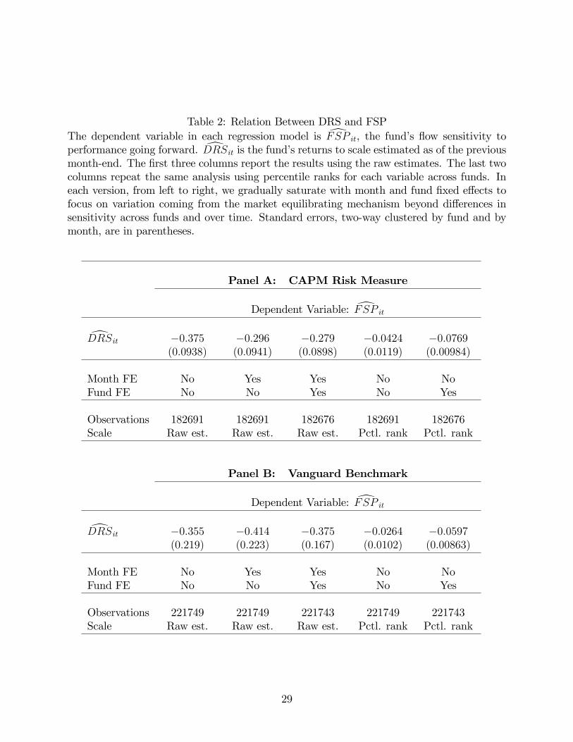
Table 2: Relation Between DRS and FSP dThe dependent variable in each regression model is F SP it, the fund’s flow sensitivity to dperformance going forward. DRSit is the fund’s returns to scale estimated as of the previous month-end. The first three columns report the results using the raw estimates. The last two columns repeat the same analysis using percentile ranks for each variable across funds. In each version, from left to right, we gradually saturate with month and fund fixed effects to focus on variation coming from the market equilibrating mechanism beyond differences in sensitivity across funds and over time. Standard errors, two-way clustered by fund and by month, are in parentheses.

Panel A: CAPM Risk Measure

dDependent Variable: F SP it

dDRSit −0.375 (0.0938)

−0.296 (0.0941)

−0.279 (0.0898)

−0.0424 (0.0119)

−0.0769 (0.00984)

Month FE Fund FE

No No

Yes No

Yes Yes

No No

No Yes

Observations Scale

182691 Raw est.

182691 Raw est.

182676 Raw est.

182691 Pctl. rank

182676 Pctl. rank

Panel B: Vanguard Benchmark

dDependent Variable: F SP it

dDRSit −0.355 (0.219)

−0.414 (0.223)

−0.375 (0.167)

−0.0264 (0.0102)

−0.0597 (0.00863)

Month FE Fund FE

No No

Yes No

Yes Yes

No No

No Yes

Observations Scale

221749 Raw est.

221749 Raw est.

221743 Raw est.

221749 Pctl. rank

221743 Pctl. rank

29

Table 3: Relation Between DRS and Size The dependent variable in each regression model is the fund’s log real AUM in $ millions d(base year is 2000). DRSit is the fund’s returns to scale estimated as of the previous month-end. Across the first three columns, we gradually saturate with month and fund fixed effects to focus on variation coming from the market equilibrating mechanism beyond differences in size across funds and over time. The last column repeats the same analysis by further including controls that are plausibly correlated with the fund size: family size, fund age, and turnover. Standard errors, two-way clustered by fund and by month, are in parentheses.

Panel A: CAPM Risk Measure

Dependent Variable: Log Real AUM

dDRSit −3.86 (1.65)

−5.23 (1.68)

−1.30 (0.558)

−1.12 (0.447)

Month FE Fund FE Controls

No No No

Yes No No

Yes Yes No

Yes Yes Yes

Observations 252420 252420 252411 247054

Panel B: Vanguard Benchmark

Dependent Variable: Log Real AUM

dDRSit −3.97 (2.20)

−5.36 (2.22)

−2.34 (0.755)

−2.66 (0.611)

Month FE Fund FE Controls

No No No

Yes No No

Yes Yes No

Yes Yes Yes

Observations 300947 300947 300936 294412

30

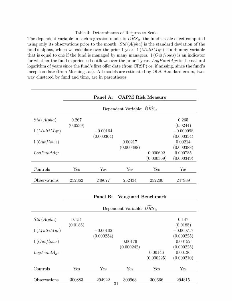
Table 4: Determinants of Returns to Scale dThe dependent variable in each regression model is DRSit, the fund’s scale effect computed using only its observations prior to the month. Std (Alpha) is the standard deviation of the fund’s alphas, which we calculate over the prior 1 year. 1 (MultiMgr) is a dummy variable that is equal to one if the fund is managed by many managers. 1 (Outflows) is an indicator for whether the fund experienced outflows over the prior 1 year. LogF undAge is the natural logarithm of years since the fund’s first offer date (from CRSP) or, if missing, since the fund’s inception date (from Morningstar). All models are estimated by OLS. Standard errors, two-way clustered by fund and time, are in parentheses.

Panel A: CAPM Risk Measure

dDependent Variable: DRSit

Std (Alpha)

1 (MultiMgr)

1 (Outflows)

LogF undAge

0.267 (0.0239)

−0.00164 (0.000364)

0.00217 (0.000398)

0.000602 (0.000369)

0.265 (0.0244) −0.000998 (0.000354) 0.00214 (0.000388) 0.000785 (0.000349)

Controls Yes Yes Yes Yes Yes

Observations 252362 248077 252434 252200 247989

Panel B: Vanguard Benchmark

dDependent Variable: DRSit

Std (Alpha)

1 (MultiMgr)

1 (Outflows)

LogF undAge

0.154 (0.0185)

−0.00102 (0.000234)

0.00179 (0.000242)

0.00146 (0.000225)

0.147 (0.0185) −0.000717 (0.000225) 0.00152 (0.000225) 0.00136 (0.000210)

Controls Yes Yes Yes Yes Yes

Observations 300883 294922 31

300963 300666 294815

Table 5: Relation Between DRS and FSP dThis table is the same as Table 2 but replaces DRSit by their predicted values based on fund gcharacteristics, DRSit.

Panel A: CAPM Risk Measure

dDependent Variable: F SP it

gDRSit −2.95 (0.568)

−2.28 (0.657)

−2.37 (0.596)

−0.0536 (0.0152)

−0.0854 (0.0148)

Month FE Fund FE

No No

Yes No

Yes Yes

No No

No Yes

Observations Scale

178624 Raw est.

178624 Raw est.

178612 Raw est.

178624 Pctl. rank

178612 Pctl. rank

Panel B: Vanguard Benchmark

dDependent Variable: F SP it

gDRSit −7.83 (1.84)

−6.88 (1.89)

−3.39 (1.99)

−0.0546 (0.0133)

−0.0404 (0.0134)

Month FE Fund FE

No No

Yes No

Yes Yes

No No

No Yes

Observations Scale

216044 Raw est.

216044 Raw est.

216040 Raw est.

216044 Pctl. rank

216040 Pctl. rank

32

Table 6: Relation Between DRS and Size dThis table is the same as Table 3 but replaces DRSit by their predicted values based on fund gcharacteristics, DRSit.

Panel A: CAPM Risk Measure

Dependent Variable: Log Real AUM

dDRSit −44.1 (8.10)

−63.3 (9.08)

−49.0 (3.83)

−36.4 (3.29)

Month FE Fund FE Controls

No No No

Yes No No

Yes Yes No

Yes Yes Yes

Observations 247975 247975 247965 243079

Panel B: Vanguard Benchmark

Dependent Variable: Log Real AUM

dDRSit −16.7 (14.9)

−16.1 (15.7)

−88.7 (7.10)

−75.5 (5.91)

Month FE Fund FE Controls

No No No

Yes No No

Yes Yes No

Yes Yes Yes

Observations 294,799 294,799 294,790 288,867

33

Table 7: Calibration The top panel summarizes the model parameters that we set directly and their parameter values. Then, for each value of b, we construct 2,500 samples of simulated panel data for 100 funds over 100 months. In each sample, we estimate the flow-performance sensitivity γ. Given b, we set σ0 so that the median of the γ estimates across simulated samples matches the flow-performance relation implied by the regression model in column 3 of Panel A of dTable 5 (i.e., F SP = 0.117 − 2.40 × DRS). Panel B contains the values of σ0 that resulted from this process for five plausible values of b: 0.00357, 0.00531, 0.00770, 0.0106, and 0.0140. These values correspond to the 10th, 25th, 50th, 75th, and 90th percentiles of fund-specific b estimates, respectively. Column 3 shows the target flow-performance sensitivities computed dusing F SP = 0.117 − 2.40 × DRS, while the resulting median of the γ estimates across simulated samples are reported in the last column. Panel C repeats the same analysis for each b, but using the counterfactual value of σ0 = 0.162% per month.

Panel A: Parameter Values Variable Symbol Value Return standard deviation σ 5.77% Exit mean θ 0%

Panel B: Calibration Parameter set Calibrated parameter F SP Decreasing returns to scale (b) Prior standard deviation (σ0) Target Model 0.00357 0.00116 0.109 0.110 0.00531 0.00139 0.105 0.107 0.00770 0.00162 0.099 0.099 0.01065 0.00186 0.092 0.093 0.01396 0.00204 0.084 0.084

Panel C: Counterfactual Parameter set Counterfactual parameter F SP Decreasing returns to scale (b) Prior standard deviation (σ0) Target Model 0.00357 0.00162 0.109 0.213 0.00531 0.00162 0.105 0.143 0.00770 0.00162 0.099 0.099 0.01065 0.00162 0.092 0.071 0.01396 0.00162 0.084 0.054

34

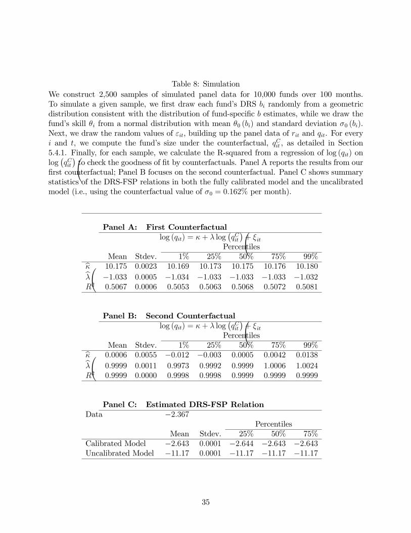
Table 8: Simulation We construct 2,500 samples of simulated panel data for 10,000 funds over 100 months. To simulate a given sample, we first draw each fund’s DRS bi randomly from a geometric distribution consistent with the distribution of fund-specific b estimates, while we draw the fund’s skill θi from a normal distribution with mean θ0 (bi) and standard deviation σ0 (bi). Next, we draw the random values of εit, building up the panel data of rit and qit. For every i and t, we compute the fund’s size under the counterfactual, qit

C , as detailed in Section 5.4.1. Finally, for each sample, we calculate the R-squared from a regression of log (qit) on � � log qit

C to check the goodness of fit by counterfactuals. Panel A reports the results from our first counterfactual; Panel B focuses on the second counterfactual. Panel C shows summary statistics of the DRS-FSP relations in both the fully calibrated model and the uncalibrated model (i.e., using the counterfactual value of σ0 = 0.162% per month).

Panel A: First Counterfactual� � log (qit) = κ + λ log qC

it + ξit Percentiles

Mean Stdev. 1% 25% 50% 75% 99% b 10.175 0.0023 10.169 10.173 10.175 10.176 10.180κ bλ −1.033 0.0005 −1.034 −1.033 −1.033 −1.033 −1.032 R2 0.5067 0.0006 0.5053 0.5063 0.5068 0.5072 0.5081

Panel B: Second Counterfactual� � log (qit) = κ + λ log qC

it + ξit Percentiles

Mean Stdev. 1% 25% 50% 75% 99% b 0.0006 −0.012 0.0005 0.0138κ 0.0055 −0.003 0.0042 bλ 0.9999 0.0011 0.9973 0.9992 0.9999 1.0006 1.0024 R2 0.9999 0.0000 0.9998 0.9998 0.9999 0.9999 0.9999

Panel C: Estimated DRS-FSP Relation Data −2.367

Percentiles Mean Stdev. 25% 50% 75%

Calibrated Model −2.643 0.0001 −2.644 −2.643 −2.643 Uncalibrated Model −11.17 0.0001 −11.17 −11.17 −11.17

35

Table 9: Relation Between Optimal Size and Fund Size

The dependent variable in each regression model is the fund’s log real AUM in $ millions (base year is 2000). qb∗ is an estimate for the optimal fund size; qb∗ is an alternative i iRD2

measure of optimal fund size, assuming that fund size has the same effect on performance for all funds. We assign funds to one of three samples based on fund age: [0, 5], (5, 10], and > 10 years. Columns 1—3 show the results from running panel regressions of log real AUM on the fund’s log optimal fund size estimate in each age-sorted sample. The last three columns

∗ ∗show the results from running multiple regressions of log (qit) on both log (qbi ) and log (qbiRD2) in all three age-sorted samples. The double clustered (by fund and time) standard errors are in parentheses.

Panel A: CAPM Risk Measure

Dependent Variable: Log Real AUM

log (qbi ∗) 0.218 0.364 0.430 −0.0189 0.00599 0.0474 (0.0158) (0.0208) (0.0330) (0.0148) (0.0110) (0.00942)

log (qb∗ ) 0.497 0.762 0.916iRD2

(0.0230) (0.0166) (0.0143)

R2 0.146 0.354 0.428 0.308 0.665 0.824

Observations 64718 105288 196233 64718 105288 196233 Fund ages [0, 5] yr. (5, 10] yr. > 10 yr. [0, 5] yr. (5, 10] yr. > 10 yr.

Panel B: Vanguard Benchmark

Dependent Variable: Log Real AUM

∗log (bq )i ∗log (bq )iRD2

0.0546 (0.00655)

0.0745 (0.00906)

0.132 (0.0166)

0.0147 (0.00472) 0.273 (0.0111)

0.0126 (0.00423) 0.484 (0.0113)

0.0251 (0.00514) 0.692 (0.0128)

R2 0.0497 0.0721 0.134 0.248 0.510 0.699

Observations Fund ages

75870 [0, 5] yr.

110319 (5, 10] yr.

196467 > 10 yr.

75870 [0, 5] yr.

110319 (5, 10] yr.

196467 > 10 yr.

36

Mean

25th pctl.

Median

75th pctl.

­.01

0.0

1.0

2.0

3D

RS 

(bp 

per l

og fu

nd A

UM

)

1990 1995 2000 2005 2010 2015Year

Panel A: CAPM risk measure

Mean

25th pctl.

Median

75th pctl.

­.01

­.005

0.0

05.0

1.0

15D

RS 

(bp 

per l

og fu

nd A

UM

)

1990 1995 2000 2005 2010 2015Year

Panel B: Vanguard Benchmark

Figure 1: Distribution of fund-specific decreasing returns to scale over time: The figure plots each month’s mean and percentiles of estimated size effect on performance across all funds operating during that month. Panel A estimates DRS using the CAPM alpha to measure fund performance. Panel B estimates DRS when we take Vanguard index funds as the alternative investment opportunity set.

37

Mean

25th pctl.

Median

75th pctl.

0.0

5.1

.15

.2.2

5FS

P (%

 per

 % a

nnua

l alp

ha)

1990 1995 2000 2005 2010 2015Year

Panel A: CAPM risk measure

Mean

25th pctl.

Median

75th pctl.

0.1

.2.3

FSP 

(% p

er %

 ann

ual a

lpha

)

1990 1995 2000 2005 2010 2015Year

Panel B: Vanguard Benchmark

Figure 2: Distribution of fund-specific flow sensitivity to performance over time: The figure plots each month’s mean and percentiles of estimated flow sensitivity to per-formance across all funds operating during that month. Panel A estimates FSP using the CAPM alpha to measure fund performance. Panel B estimates FSP when net alpha is computed using Vanguard index funds as benchmark portfolios.

38

Mean

25th pctl.

Median

75th pctl.

.005

.01

.015

.02

Cha

ract

eris

tic­b

ased

 DR

S (b

p pe

r log

 fund

 AU

M)

1990 1995 2000 2005 2010 2015Year

Panel A: CAPM risk measure

Mean

25th pctl.

Median

75th pctl.

.002

.004

.006

.008

Cha

ract

eris

tic­b

ased

 DR

S (b

p pe

r log

 fund

 AU

M)

1990 1995 2000 2005 2010 2015Year

Panel B: Vanguard Benchmark

Figure 3: Cross-sectional distribution of characteristic-based DRS over time: This dfigure is the same as Figure 1 but measures size effect on performance not by DRSit, but by gtheir predicted values based on fund characteristics, DRSit.

39

0 0.005 0.01 0.015 0.02 0.025 b

0

0.05

0.1

0.15

0(b)

Panel A: Prior mean as a function of DRS

0 0.005 0.01 0.015 0.02 0.025 b

0.5

1

1.5

2

2.5

0(b)

10­3 Panel B: Prior uncertainty as a function of DRS

Figure 4: Priors, conditional on the fund’s decreasing returns to scale parameter b: Panel A plots the prior mean (θ0) as a function of b that we use in our simulation analysis. Panel B plots the prior uncertainty (σ0) as a function of b that we use in our simulation analysis. Given b, σ0 is calibrated so that the median of the FSP (flow sensitivity to performance) estimates across simulated samples matches the flow-performance relation implied by the regression model in column 3 of Panel A of Table 5. Our approach is to calibrate the prior uncertainty for 100 disperse values of b, fitting a quadratic polynomial to the data, (b, σ0), that resulted from this process to extrapolate the prior uncertainty, conditional on other values of b, that we use in our simulation analysis.

40

02

46

810

Opt

imal

 Log

 Siz

e Ba

sed 

on F

und­

Spec

ific 

DR

S

0 2 4 6 8 10Optimal Log Size Assuming the Same DRS Value

Panel A: CAPM risk measure­5

05

10O

ptim

al L

og S

ize 

Base

d on

 Fun

d­Sp

ecifi

c D

RS

­5 0 5 10Optimal Log Size Assuming the Same DRS Value

Panel B: Vanguard Benchmark

Figure 5: Relation between two measures of optimal fund size: The figure plots the main measure of optimal fund size, log (qbi ∗), versus the alternative measure of optimal fund

∗ ∗size, log (qbiRD2). We compute the optimal fund size, qbi , by estimating fund-specific a and b parameters. We construct an alternative measure of optimal log fund size, ignoring the fact that there is individual heterogeneity in decreasing returns to scale. The circles represent pairs of (log (qb∗ ) , log (qb∗)). The red line depicts the identity line. iRD2 i

41