Embed Size (px)
Citation preview
Review of Economic Studies (2012) 00, 1–40 0034-6527/12/00000001$02.00
c© 2012 The Review of Economic Studies Limited
Capital Flows to Developing Countries:The Allocation Puzzle1
PIERRE-OLIVIER GOURINCHAS
University of California Berkeley, SciencesPo, NBER & CEPRE-mail: [email protected]
OLIVIER JEANNE
Johns Hopkins University, NBER, CEPR & Peterson InstituteE-mail: [email protected]
First version received June 2009; final version accepted August 2012 (Eds.)
The textbook neoclassical growth model predicts that countries with fasterproductivity growth should invest more and attract more foreign capital. We show thatthe allocation of capital flows across developing countries is the opposite of this prediction:capital does not flow more to countries that invest and grow more. We call this puzzlethe “allocation puzzle.” Using a wedge analysis, we find that the pattern of capital flows isdriven by national saving: the allocation puzzle is a saving puzzle. Further disaggregation ofcapital flows reveals that the allocation puzzle is also related to the pattern of accumulationof international reserves. The solution to the “allocation puzzle”, thus, lies at the nexusbetween growth, saving and international reserve accumulation. We conclude with adiscussion of some possible avenues for research.
1. INTRODUCTION
The role of international capital flows in economic development raises important openquestions. In particular, the question asked by Robert Lucas twenty years ago—why solittle capital flows from rich to poor countries—received renewed interest in recent yearsas capital has been flowing “upstream” from developing countries to the U.S. since 2000.1
This paper takes a fresh look at the pattern of net capital flows to developingcountries through the lenses of the neoclassical growth model. We show that there isa significant discrepancy between the predictions of the textbook neoclassical growthmodel and the distribution of capital flows across developing countries observed in thedata. The basic framework predicts that countries that enjoy higher productivity growthshould receive more net capital inflows. We look at net capital inflows for a large sampleof non-OECD countries over the period 1980-2000 and find that this is not true. In factthe cross-country correlation between productivity growth and net capital inflows is often
1. We would like to thank our editor and referees at the Review, Philippe Bacchetta, ChrisCarroll, Francesco Caselli, Kerstin Gerling, Peter Henry, Sebnem Kalemli-Ozcan, Pete Klenow, AlbertoMartin, Romain Ranciere, Assaf Razin, Damiano Sandri, Federico Sturzenegger for useful commentsand especially Chang-Tai Hsieh and Chad Jones for insightful discussions. We also thank variousseminar participants. A first draft of this paper was completed while the second author was visitingthe Department of Economics of Princeton University, whose hospitality is gratefully acknowledged.Pierre-Olivier Gourinchas thanks the NSF (grants SES-0519217 and SES-0519242) and the ICG (GrantRA-2009-11-002) for financial support.
1. See Lucas (1990) for the seminal article and Prasad et al. (2007) on the upstream flows ofcapital.
1
2 REVIEW OF ECONOMIC STUDIES
AGO
ARG
BEN
BGD
BOL
BRA
BWA
CHL
CHN
CIV
CMR
COG
COL
CRICYP
DOMECU
EGYETH
FJI
GAB
GHAGTM
HKG
HND
HTI
IDN IND
IRN
ISR
JAM
JOR KEN
LKA
MARMEX
MLI
MOZ
MUS
MWI
MYS
NER
NGA
NPL
PAK
PAN
PER
PHLPNG
PRYRWA
SEN
SGP
SLV
SYR
TGO
THA
TTO
TUN
TUR
TWN
TZA
UGA
URY
VEN
ZAF KOR
MDG
−1
0−
50
51
01
5C
ap
ita
l In
flo
ws (
pe
rce
nt
of
GD
P)
−4 −2 0 2 4 6Productivity Growth (%)
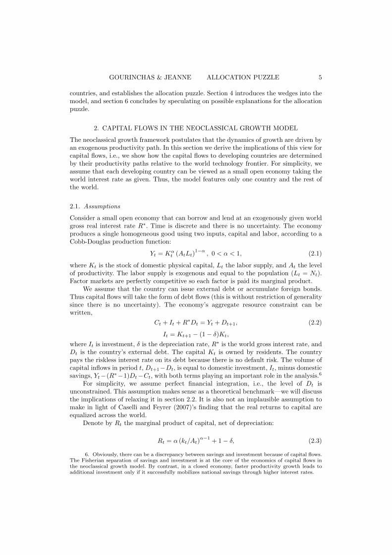
Figure 1
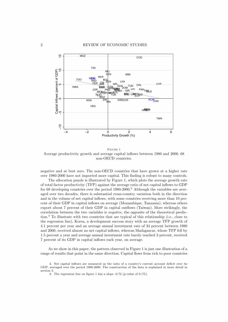
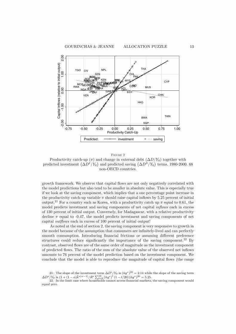
Average productivity growth and average capital inflows between 1980 and 2000. 68non-OECD countries.
negative and at best zero. The non-OECD countries that have grown at a higher rateover 1980-2000 have not imported more capital. This finding is robust to many controls.
The allocation puzzle is illustrated by Figure 1, which plots the average growth rateof total factor productivity (TFP) against the average ratio of net capital inflows to GDPfor 68 developing countries over the period 1980-2000.2 Although the variables are aver-aged over two decades, there is substantial cross-country variation both in the directionand in the volume of net capital inflows, with some countries receiving more than 10 per-cent of their GDP in capital inflows on average (Mozambique, Tanzania), whereas othersexport about 7 percent of their GDP in capital outflows (Taiwan). More strikingly, thecorrelation between the two variables is negative, the opposite of the theoretical predic-tion.3 To illustrate with two countries that are typical of this relationship (i.e., close tothe regression line), Korea, a development success story with an average TFP growth of4.1 percent per year and an average annual investment rate of 34 percent between 1980and 2000, received almost no net capital inflows, whereas Madagascar, whose TFP fell by1.5 percent a year and average annual investment rate barely reached 3 percent, received7 percent of its GDP in capital inflows each year, on average.
As we show in this paper, the pattern observed in Figure 1 is just one illustration of arange of results that point in the same direction. Capital flows from rich to poor countries
2. Net capital inflows are measured as the ratio of a country’s current account deficit over itsGDP, averaged over the period 1980-2000. The construction of the data is explained in more detail insection 3.
3. The regression line on figure 1 has a slope -0.72 (p-value of 0.1%).
GOURINCHAS & JEANNE ALLOCATION PUZZLE 3
are not only low (as argued by Lucas (1990)), but their allocation across developingcountries is negatively correlated or uncorrelated with the predictions of the standardtextbook model. This is the “allocation puzzle.”
We provide a more detailed characterization of the allocation puzzle by looking atdifferent breakdowns (decompositions) of capital flows. First, we delineate the respectiveroles of investment and saving. We augment the neoclassical growth model with two“wedges”: one wedge that distorts investment decisions, and one wedge that distortssaving decisions. It is then possible, for each country in our sample, to estimate thesaving and investment wedges that are required to explain the observed levels of savingsand investment (and therefore of net capital flows). We find that the investment wedgecannot, by itself, explain the allocation puzzle, and that solving the allocation puzzlerequires a saving wedge that is strongly negatively correlated with productivity growth.That is, the allocation puzzle is a saving puzzle.
We then look at a decomposition of international capital flows into public andprivate flows similar to Aguiar and Amador (2011). We confirm that paper’s findingthat the allocation puzzle is mostly a feature of public flows, and in addition find thatthe accumulation of international reserves plays a role in generating the puzzle. However,we do not find robust evidence that private flows conform to the predictions of theory.
What can explain this puzzling allocation of capital flows across developingcountries? Our wedge analysis shows that the explanation must involve the relationshipbetween savings and growth, and our flow decomposition suggests that reserveaccumulation plays an important role. This suggests to us that the solution to theallocation puzzle should be looked for at the nexus between growth, saving, and reserveaccumulation. Why do countries that grow more also accumulate more reserves, andwhy is this reserve accumulation not offset by capital inflows to the private sector? Wediscuss possible explanations at the end of the paper—some of which were developedsince the first version of this paper was circulated. No attempt is made to discriminateempirically between these explanations —the objective of the last section of the paperbeing to propose a road map for future research rather than to establish new results.
This paper lies at the confluence of different lines of literature. First, it is related tothe literature on the determinants of capital inflows to developing countries, and on theirrole in economic development. Aizenman et al. (2007) construct a self-financing ratioindicating what would have been the counterfactual stock of capital in the absence ofcapital inflows. They find that 90 percent of the stock of capital in developing countries isself-financed, and that countries with higher self-financing ratios grew faster in the 1990s.Prasad et al. (2007) also document a negative cross-country correlation between the ratioof capital inflows to GDP and growth, and discuss possible explanations for this finding.Manzocchi and Martin (1997) empirically test an equation for capital inflows derived froman open-economy growth model on cross-section data for 33 developing countries—andfind relatively weak support.
The paper is also related to the literature on savings, growth, and investment.That literature has established a positive correlation between savings and growth, apuzzling fact from the point of view of the permanent income hypothesis since high-growth countries should borrow abroad against future income to finance a higher levelof consumption (Carroll and Summers (1991), Carroll and Weil (1994)). Starting withFeldstein and Horioka (1980), the literature has also established a strongly positivecorrelation between savings and investment. The allocation puzzle presented in this paperis related to both puzzles, but it is stronger. Our finding is that the difference betweensavings and investment (capital outflows) is positively correlated with productivity
4 REVIEW OF ECONOMIC STUDIES
growth.This paper is also related to the literature on the relationship between growth and the
current account in developing countries. Emerging market business cycles exhibit countercyclical current accounts, i.e., the current account balance tends to decrease when growthpicks up (see Aguiar and Gopinath (2007)). We show in this paper that the cross-countrycorrelation between growth and the current account is the opposite. Because of the verylow frequency at which we look at the data, a more natural benchmark of comparison isthe literature on transitional growth dynamics pioneered by Mankiw et al. (1992). Kingand Rebelo (1993b) also examine transition dynamics in a variety of neoclassical growthmodels. Unlike these papers, we allow countries to catch-up or fall behind relative to theworld technology frontier and focus on the implications of the theory for internationalcapital flows.
Our wedge analysis is similar to Chari et al. (2007)’s “business cycle accounting.”Those authors show that a large class of dynamic stochastic general equilibrium modelsare observationally equivalent to a benchmark real business cycle model with correlated“wedges” in their first-order conditions. The main difference is that while Chari et al.(2007) look at real business fluctuations, we focus here on long-term growth. In a moreclosely related contribution, Chari et al. (1996) show that a neoclassical growth modelwith investment distortions does fairly well in accounting for the observed distributionof income and the patterns of investment across countries.
Finally, this paper belongs to a small set of contributions that look at theimplications of the recent “development accounting” literature for internationaleconomics. Development accounting has implications for the behavior of capitalflows that have not been systematically explored in the literature (by contrast withinvestment, whose relationship with productivity is well understood and documented).Two conclusions from this literature are especially relevant for our analysis. First, asubstantial share of the cross-country inequality in income per capita comes from cross-country differences in TFP —see Hall and Jones (1999) and the subsequent literatureon development accounting reviewed in Caselli (2005). The economic take-off of a poorcountry, therefore, results from a convergence of its TFP toward the level of advancedeconomies. Second, developing countries are able to accumulate the level of productivecapital that is warranted by their level of TFP. Caselli and Feyrer (2007) show that thereturn to capital, once properly measured in a development accounting framework, isvery similar in advanced and developing countries.4 If we accept these conclusions, thenan open economy version of the basic neoclassical growth model should be a reasonabletheoretical benchmark to think about the behavior of capital flows toward developingcountries. The present paper is the first, to our knowledge, to quantify the level of capitalflows to developing countries in a calibrated open economy growth model and compareit with the data.5
The paper is structured as follows. Section 2 presents the model that we use topredict the volume and allocation of capital flows to developing countries. Section 3 thencalibrates the model using Penn World Table (PWT) data on a large sample of developing
4. Caselli and Feyrer (2007) consider a neoclassical growth framework similar to the model usedhere but do not look at the channels through which the returns to capital are equalized. By contrast, welook at the capital flows that are required to equalize those returns in the neoclassical framework.
5. In Gourinchas and Jeanne (2006) we use a development accounting framework similar to thatin this paper to quantify the welfare gains from capital mobility, and find them to be relatively small.We do not compare the predictions of the model with the observed capital flows to developing countriesas we do here.
GOURINCHAS & JEANNE ALLOCATION PUZZLE 5
countries, and establishes the allocation puzzle. Section 4 introduces the wedges into themodel, and section 6 concludes by speculating on possible explanations for the allocationpuzzle.
2. CAPITAL FLOWS IN THE NEOCLASSICAL GROWTH MODEL
The neoclassical growth framework postulates that the dynamics of growth are driven byan exogenous productivity path. In this section we derive the implications of this view forcapital flows, i.e., we show how the capital flows to developing countries are determinedby their productivity paths relative to the world technology frontier. For simplicity, weassume that each developing country can be viewed as a small open economy taking theworld interest rate as given. Thus, the model features only one country and the rest ofthe world.
2.1. Assumptions
Consider a small open economy that can borrow and lend at an exogenously given worldgross real interest rate R∗. Time is discrete and there is no uncertainty. The economyproduces a single homogeneous good using two inputs, capital and labor, according to aCobb-Douglas production function:
Yt = Kαt (AtLt)
1−α, 0 < α < 1, (2.1)
where Kt is the stock of domestic physical capital, Lt the labor supply, and At the levelof productivity. The labor supply is exogenous and equal to the population (Lt = Nt).Factor markets are perfectly competitive so each factor is paid its marginal product.
We assume that the country can issue external debt or accumulate foreign bonds.Thus capital flows will take the form of debt flows (this is without restriction of generalitysince there is no uncertainty). The economy’s aggregate resource constraint can bewritten,
Ct + It +R∗Dt = Yt +Dt+1, (2.2)
It = Kt+1 − (1− δ)Kt,
where It is investment, δ is the depreciation rate, R∗ is the world gross interest rate, andDt is the country’s external debt. The capital Kt is owned by residents. The countrypays the riskless interest rate on its debt because there is no default risk. The volume ofcapital inflows in period t, Dt+1−Dt, is equal to domestic investment, It, minus domesticsavings, Yt−(R∗−1)Dt−Ct, with both terms playing an important role in the analysis.6
For simplicity, we assume perfect financial integration, i.e., the level of Dt isunconstrained. This assumption makes sense as a theoretical benchmark—we will discussthe implications of relaxing it in section 2.2. It is also not an implausible assumption tomake in light of Caselli and Feyrer (2007)’s finding that the real returns to capital areequalized across the world.
Denote by Rt the marginal product of capital, net of depreciation:
Rt = α (kt/At)α−1
+ 1− δ, (2.3)
6. Obviously, there can be a discrepancy between savings and investment because of capital flows.The Fisherian separation of savings and investment is at the core of the economics of capital flows inthe neoclassical growth model. By contrast, in a closed economy, faster productivity growth leads toadditional investment only if it successfully mobilizes national savings through higher interest rates.
6 REVIEW OF ECONOMIC STUDIES
where kt denotes capital per capita and more generally, lower case variables arenormalized by population. Capital mobility implies that the private return on domesticcapital and the world real interest rate are equal: Rt = R∗. Substituting this into theexpression for the gross return on capital (2.3), we obtain that the capital stock perefficient unit of labor k = kt/At is constant and equal to:
kt = k∗ ≡(
α
R∗ + δ − 1
)1/1−α
, (2.4)
where ‘tilde-variables’ denote per capita variables in efficiency units: k = K/AN .The country has an exogenous, deterministic productivity path (At)
∞t=0, which is
bounded from above by the world productivity frontier,
At ≤ A∗t = A∗0g∗t.
The world productivity frontier reflects the advancement of knowledge, which is notcountry specific, and is assumed to grow at a constant rate g∗.
Domestic productivity could grow at a rate that is higher or lower than g∗ for afinite period of time. In order to describe how domestic productivity evolves relative tothe world frontier, it is convenient to define πt as the gap between domestic productivityand the productivity in the absence of technological catch-up,
πt ≡At
A0g∗t− 1.
We assume that π = limt→∞ πt is well defined. Domestic productivity convergesto a fraction of the world frontier, and the limit π measures the country’s long-run technological catch-up relative to that frontier. If π = 0, the country’s long-runproductivity remains unchanged relative to the world frontier. If π > 0, the countrycatches up relative to the frontier, and if π < 0, the country falls further behind. Thecountry’s productivity growth rate always converges to g∗.7
Next, we need to make some assumptions about the determination of domesticconsumption and savings. Here, we adopt the textbook Cass-Ramsey model extendedto accommodate a growing population. The population Nt grows at an exogenous rate n:Nt = ntN0. Like in Barro and Sala-i-Martin (1995) we assume that the population canbe viewed as a continuum of identical families whose representative member maximizesthe welfare function:
Ut =
∞∑s=0
βs Nt+s u (ct+s) , (2.5)
where u (c) ≡(c1−γ − 1
)/ (1− γ) is a constant relative risk aversion (CRRA) utility
function with coefficient γ > 0. The number of families is normalized to 1, so that perfamily and aggregate variables are the same.
The budget constraint of the representative family is given by:
Ct +Kt+1 = R∗(Kt −Dt) +Dt+1 +Ntwt, (2.6)
where wt is the wage, equal to the marginal product of labor (1− α) kαt A1−αt .
7. That countries have the same growth rate in the long run is a standard assumption, oftenjustified by the fact that no country should have a share of world GDP converging to 0 or 100 percent.Models of idea flows such as Parente and Prescott (2000) or Eaton and Kortum (1999) imply a commonlong-run growth rate of productivity.
GOURINCHAS & JEANNE ALLOCATION PUZZLE 7
The representative resident maximizes the welfare function (2.5) subject to thebudget constraint (2.6). The Euler equation for the small open economy is,
c−γt = βR∗c−γt+1. (2.7)
We assume that the world interest factor is given by,
R∗ = g∗γ/β. (2.8)
Equation (2.8) holds if the rest of the world is composed of advanced economies thathave the same preferences as the small economy under consideration, and have alreadyachieved their steady state. This is a natural assumption to make, given that we lookat the impact on capital flows of cross-country differences in productivity, rather thanpreferences.
A country is characterized by an initial capital stock per capita k0, debt per capitad0, population growth rate n, and a productivity path {At}∞t=0. We assume that allcountries are financially open at time t = 0 and use the model to estimate the size andthe direction of capital flows from t = 0 onward.
2.2. Productivity and capital flows
We compare the predictions of the model with the data observed over a finite period oftime denoted [0, T ]. We abstract from unobserved future developments in productivityby assuming that all countries have the same productivity growth rate, g∗, after time T .We further assume that the path for the ratio πt/π is the same for all countries and isgiven by:
πt = πf(t), (2.9)
where f(·) is common across countries and satisfies f(t) ≤ 1 and f(t) = 1 for t ≥ T . Thisassumption allows us to characterize the productivity differences between countries witha single parameter, the long-run productivity catch-up coefficient π.
Next, we need to define an appropriate measure of capital inflows during the timeinterval [0, T ]. A natural measure, in our model, is the change in external debt between0 and T normalized by initial GDP,
∆D
Y0=DT −D0
Y0. (2.10)
The normalization by initial GDP ensures that the measure is comparable acrosscountries of different sizes.8
The following proposition characterizes how the direction and volume of capital flowsdepend on the exogenous parameters of the model.
8. Capital inflows could be measured in different ways, for example as the average ratio of netcapital inflows to GDP (like in Figure 1) or as the change in the ratio of net foreign liabilities to GDP.In Gourinchas and Jeanne (2007) we show that the predictions of the model are qualitatively the samefor the three measures of capital flows. Moreover, we show that if the allocation puzzle is observed withmeasure (2.10) then it must also hold with the two other measures. This is another reason to use measure(2.10) as a benchmark when we look at the data.
8 REVIEW OF ECONOMIC STUDIES
Proposition 1. Under assumptions (2.1), (2.2), (2.5), (2.8) and (2.9), the ratioof cumulated net capital inflows to initial output between t = 0 and t = T is given by:
∆D
Y0=
∆Dc/Y0︷ ︸︸ ︷k∗ − k0
y0(ng∗)
T+
∆Dt/Y0︷ ︸︸ ︷d0
y0
[(ng∗)
T − 1]
(2.11)
+
∆Di/Y0︷ ︸︸ ︷πk∗
y0(ng∗)
T+
∆Ds/Y0︷ ︸︸ ︷π
w
R∗y0(ng∗)
TT−1∑t=0
(ng∗
R∗
)t[1− f(t)] .
Net capital inflows are increasing in the productivity catch-up parameter (π),decreasing in the initial level of capital (k0) and, when trend growth is positive (ng∗ > 1),increasing in the initial level of debt (d0).
Proof. See appendix A
Equation (2.11) implies that a country without capital scarcity (k0 = k∗), withoutinitial debt (d0 = 0) and without productivity catch-up (π = 0) has no net capital flows.Consider now each term on the right-hand side of equation (2.11) in turn.
The first term, ∆Dc/Y0, results from the initial level of capital scarcity k∗ − k0.Under financial integration, and in the absence of financial frictions or adjustment costof capital, the country instantly borrows and invests the amount k∗ − k0. We call thisterm the convergence term.
The second term, ∆Dt/Y0, reflects the impact of initial debt. In the absence ofproductivity catch-up the economy follows a balanced growth path in which externaldebt remains a constant fraction of output. The cumulated debt inflows that are requiredto keep the debt-to-output ratio constant are equal to ∆Dt and increase with the debt-to-output ratio when trend growth is positive (ng∗ > 1). We call this term the trendterm.
The third and fourth terms in (2.11) reflect the impact of the productivity catch-up.The third term, ∆Di/Y0, represents the external borrowing that goes toward financingdomestic investment. To see this, observe that since capital per efficient unit of laborremains constant at k∗, capital per capita k = kA needs to increase more when thereis a productivity catch-up. Without productivity catch-up, capital at time T would bek∗NTA0g
∗T . Instead, it is k∗NTAT . The difference, πk∗NTA0g∗T , normalized by output
y0A0N0, is equal to ∆Di/Y0. This is the investment term.Finally, the fourth term, ∆Ds/Y0, represents the change in external debt brought
about by changes in domestic saving. It is proportional to normalized labor income (herethe wage w) and to the long-run productivity catch-up π. Faster relative productiv-ity growth implies higher future income, leading to an increase in consumption and adecrease in savings. Since current income is unchanged, the representative domestic con-sumer borrows on the international markets. This is the saving term.
The proposition immediately implies the following corollary.
Corollary 1. Under the assumptions of proposition 1,
GOURINCHAS & JEANNE ALLOCATION PUZZLE 9
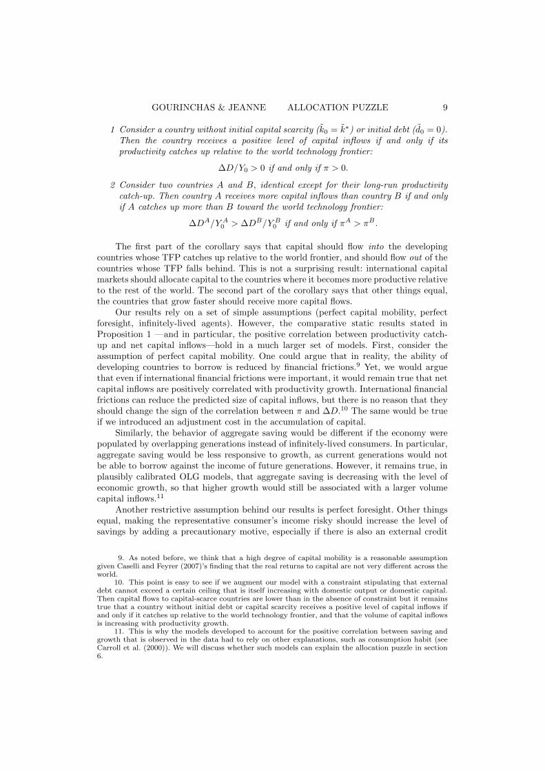
1 Consider a country without initial capital scarcity (k0 = k∗) or initial debt (d0 = 0).Then the country receives a positive level of capital inflows if and only if itsproductivity catches up relative to the world technology frontier:
∆D/Y0 > 0 if and only if π > 0.
2 Consider two countries A and B, identical except for their long-run productivitycatch-up. Then country A receives more capital inflows than country B if and onlyif A catches up more than B toward the world technology frontier:
∆DA/Y A0 > ∆DB/Y B0 if and only if πA > πB .
The first part of the corollary says that capital should flow into the developingcountries whose TFP catches up relative to the world frontier, and should flow out of thecountries whose TFP falls behind. This is not a surprising result: international capitalmarkets should allocate capital to the countries where it becomes more productive relativeto the rest of the world. The second part of the corollary says that other things equal,the countries that grow faster should receive more capital flows.
Our results rely on a set of simple assumptions (perfect capital mobility, perfectforesight, infinitely-lived agents). However, the comparative static results stated inProposition 1 —and in particular, the positive correlation between productivity catch-up and net capital inflows—hold in a much larger set of models. First, consider theassumption of perfect capital mobility. One could argue that in reality, the ability ofdeveloping countries to borrow is reduced by financial frictions.9 Yet, we would arguethat even if international financial frictions were important, it would remain true that netcapital inflows are positively correlated with productivity growth. International financialfrictions can reduce the predicted size of capital inflows, but there is no reason that theyshould change the sign of the correlation between π and ∆D.10 The same would be trueif we introduced an adjustment cost in the accumulation of capital.
Similarly, the behavior of aggregate saving would be different if the economy werepopulated by overlapping generations instead of infinitely-lived consumers. In particular,aggregate saving would be less responsive to growth, as current generations would notbe able to borrow against the income of future generations. However, it remains true, inplausibly calibrated OLG models, that aggregate saving is decreasing with the level ofeconomic growth, so that higher growth would still be associated with a larger volumecapital inflows.11
Another restrictive assumption behind our results is perfect foresight. Other thingsequal, making the representative consumer’s income risky should increase the level ofsavings by adding a precautionary motive, especially if there is also an external credit
9. As noted before, we think that a high degree of capital mobility is a reasonable assumptiongiven Caselli and Feyrer (2007)’s finding that the real returns to capital are not very different across theworld.
10. This point is easy to see if we augment our model with a constraint stipulating that externaldebt cannot exceed a certain ceiling that is itself increasing with domestic output or domestic capital.Then capital flows to capital-scarce countries are lower than in the absence of constraint but it remainstrue that a country without initial debt or capital scarcity receives a positive level of capital inflows ifand only if it catches up relative to the world technology frontier, and that the volume of capital inflowsis increasing with productivity growth.
11. This is why the models developed to account for the positive correlation between saving andgrowth that is observed in the data had to rely on other explanations, such as consumption habit (seeCarroll et al. (2000)). We will discuss whether such models can explain the allocation puzzle in section6.
10 REVIEW OF ECONOMIC STUDIES
constraint. This would not change the fact, however, that the representative household iswilling to borrow against future income, and so the model would still predict a negative(positive) correlation between saving (capital inflows) and expected trend growth.12
Thus, the neoclassical growth framework makes a very robust prediction for the signof the correlation between productivity growth and capital inflows. Countries that growat a higher rate should receive more capital inflows. We now proceed to look at thiscorrelation in the data.
3. THE ALLOCATION PUZZLE
Do developing countries with faster productivity growth, larger initial capital scarcity, orlarger initial debt level receive more capital flows? We answer this question by comparing,for each country in our sample, the model predictions with observed net capital flows.
3.1. Calibrating the model
The benchmark calibration of the model follows the development accounting literature(see Caselli (2005)). We set the depreciation rate of physical capital δ to 0.06 and thecapital share α to 0.3. Differences across countries arise from differences in initial capitalk0, in the growth rate of working-age population n and in the productivity catch-upterm π. The productivity catch-up is measured relative to a world productivity frontier.We assume that the world productivity frontier corresponds to the U.S. total factorproductivity, so that g∗ = 1.017, the observed growth of U.S. total factor productivitybetween 1980 and 2000.
The calibration of the model requires also an estimate of the world interest rateR∗. In anticipation of the next section of the model, we obtain R∗ by setting β = 0.96and assuming log preferences (γ = 1). Our choice of the discount factor is consistentwith the estimates of Gourinchas and Parker (2002). Our assumption of log-preferencesis rather conservative, given the uncertainty about whether the intertemporal elasticityof substitution is larger or smaller than one. Under these assumptions, equation (2.8)implies a world interest rate equal to R∗ = 1.017/0.96 = 1.0594. This seems a reasonablenumber. For instance, Caselli and Feyrer (2007) report an average marginal return tocapital of 6.9 percent for poor countries, with a standard deviation of 3.7 percent. Wediscuss alternate calibrations in section 3.3. Lastly, for simplicity we assume that theproductivity catch-up function f(.) follows a piecewise linear path: f(t) = min (t/T, 1).
3.2. Measuring productivity growth and capital flows
We focus on the period 1980-2000. This choice of period is motivated by twoconsiderations. First, we want a period where countries were financially open. Indicatorsof financial openness show a sharp increase starting in the late 1980s and early 1990s.For instance, the Chinn and Ito (2008) index indicates an average increase in financialopenness from -0.38 in 1980 to 0 in 2000 for the countries in our sample.13 Second, wewant as long a sample as possible, since the focus is on long-term capital flows. Resultsover shorter periods may be disproportionately affected by a financial crisis in some
12. Things could be different if higher growth is associated with higher risk—we will come back tothat point in section 6.
13. The index runs from -2.6 (most closed) to 2.6 (most open) with mean 0.
GOURINCHAS & JEANNE ALLOCATION PUZZLE 11
countries or by fluctuations in the world business cycle. Our final sample consists of 68developing countries: 65 non-OECD countries, as well as Korea, Mexico and Turkey.14
We measure productivity growth following the method that has become standardin the development accounting literature. First we estimate n for each country as theannual growth rate of the working-age population.15 The other country-specific data arethe paths for output, capital and productivity. Those data come from Version 6.1 ofthe Penn World Tables (Heston et al. (2004)). The capital stock Kt is constructed withthe perpetual inventory method from time series data on real investment (also from thePenn World Tables).16 From equation (2.1), we obtain the level of productivity At as
(yt/kαt )
1/(1−α), and the level of capital stock per efficient unit of labor kt as (kt/yt)
1/(1−α).
The productivity catch-up parameter, π, is then measured as A2000/(g∗20A1980)−1, where
At is obtained as the trend component of the Hodrick-Prescott filter of At.17
We then construct, for each country, the volume of capital inflows between 1980 and2000 in terms of initial GDP,
∆D
Y0=D2000 −D1980
Y1980.
The estimate of the initial net external debt in U.S. dollar (D0) is obtained fromLane and Milesi-Ferretti (2007)’s External Wealth of Nations Mark II database (EWN),as the difference between (the opposite of) the reported net international investmentposition (NIIP) and the errors and omissions (EO) cumulated between 1970 and 1980.We measure net capital inflows in current U.S. dollars using IMF’s International FinancialStatistics data on current account deficits, keeping with the usual practice that considerserrors and omissions as unreported capital flows. We need an appropriate price indexto convert both measures into constant international dollars, the unit used in the PennWorld Tables for real variables such as output and capital stocks. In principle, the tradeand current account balances should be deflated by the price of traded goods, but thePenn World Tables do not report this price index. We use instead the price of investmentgoods which is reported in the Penn World Tables. This seems to be a good proxy becauseinvestment goods are mostly tradable—as suggested by the fact that their price variesless across countries than that of consumption goods. The PPP adjustment tends toreduce the estimated size of capital flows relative to output in poor countries, becausethose countries have a lower price of output (see Hsieh and Klenow (2007)). Appendix Bprovides additional details.
One advantage of our PPP-adjusted estimates of cumulated capital flows is thatthey can be compared to the measures of output or capital accumulation used in thedevelopment accounting literature. The allocation puzzle, however, does not hinge on
14. We will sometimes refer to the countries in our sample simply as non-OECD countries. For asmall set of countries, the sample period starts later and/or end earlier, due to data availability. The listof countries and sample period are reported in appendix C.
15. Working-age population (typically ages 15-64) is constructed using United Nations data onWorld Population Prospects.
16. See Caselli (2005) for details. Following standard practice, we set initial capital to I/ (gi + δ)where I is the initial investment level from the Penn World Tables and gi is the rate of growth of realinvestment for the first 10 years of available data.
17. We set the smoothing parameter to 1600. With annual data, this filters out more than 70percent of cycles of periodicity lower than 32 years ensuring a very smooth trend productivity. See Kingand Rebelo (1993a).
12 REVIEW OF ECONOMIC STUDIES
the particular assumptions that we make in constructing those estimates. We tried otherdeflators, which did not affect the thrust of our results.18
3.3. Correlation between productivity growth and capital flows
Table 1 presents estimates for the productivity catch-up parameters and capital flows forthe whole sample as well as regional and income groups. The estimates of π reported incolumn (1) show that there is no overall productivity catch-up with advanced countries:π is slightly negative on average. Thus we should not expect a lot of capital to flowfrom advanced to developing countries. Yet, closer inspection reveals an interestinggeographical pattern. There was a sizeable productivity catch-up in Asia (π = 0.19),while Latin America and Africa fell behind (π = −0.24 and −0.17 respectively).19 Sowhile we should not expect substantial capital inflows into developing countries as awhole, we should expect international capital to flow out of Africa and Latin America,and into Asia.
This does not seem to be the case in the data. Column (2) of Table 1 reports observednet capital inflows as a fraction of initial output, ∆D/Y0. Africa received slightly lessthan 40 percent of its initial output in capital flows. Similarly, capital flows to LatinAmerica amounted to 37 percent of its initial output, in spite of a significant relativeproductivity decline. By contrast, Asia, whose productivity grew at the highest rate,borrowed over that period only 11 percent of its initial output.
The same pattern is evident if we group countries by income levels rather thanregions. According to Table 1, poorer countries experienced lower productivity catch-upand so should export more capital according to Corollary 1. Observed capital inflows runin the exact opposite direction: actual capital flows decrease with income per capita, from56 percent of output for low income countries to -58 percent for high-income non-OECDcountries.
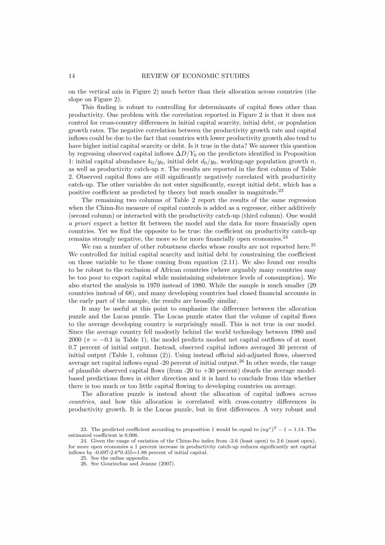
Figure 2 gives a broader cross-country perspective on the discrepancy between themodel predictions and the data by plotting observed capital inflows against observedproductivity catch-up for the full country sample, together with the relationship thatshould have been observed (according to the model) based on the investment term∆Di/Y0 (solid line with triangles) and the saving term ∆Ds/Y0 (dashed line withcircles). The model predictions are computed assuming that there is no initial debt orcapital scarcity (d0 = 0 and k0 = k∗) and using the average growth rate of working-age population in our sample: n = 1.0214. Under these assumptions, predicted total netinflows is the sum of the investment and saving terms in equation (2.11) where each termis linear in the productivity catch-up coefficient.
One observes immediately that most countries are located in the ‘wrong’ quadrantof the figure, with negative productivity catch-up but positive capital inflows. Indeed,the empirical correlation between productivity catch-up and capital inflows is negativeand statistically significant at the 1 percent level.20
In addition to confirming, with different measures, the basic correlation alreadyshown in Figure 1, Figure 2 compares the data to the prediction of the basic neoclassical
18. For instance, results are similar when using the price of output as a deflator. See the onlineappendix.
19. This pattern does not apply uniformly to all countries within a region. For instance, π = −0.34for the Philippines, 0.28 for Chile and 0.47 for Botswana.
20. The slope of the regression line in figure 2 is -0.68 with a s.e. of 0.18 (p-value smaller than0.01).
GOURINCHAS & JEANNE ALLOCATION PUZZLE 13
KOR
TWN
BGD
HKG
PNG
CHN
IDNPHL
SGP
LKA
PAK
FJI INDTUR
MYS
THANPL
BOL
PAN
VEN
HTI
COLPRYCRIMEXSLVTTO
PER
ARG
URYBRAGTM DOM
JAM
HNDECU
CHL
ISRBEN
NGA
MOZ
TGO
TZAJOR
CIV
MAR MUSIRN
MLI
COG
SYRZAF
NER MWIGHA
RWA
AGOSEN
KEN
MDG UGA
BWA
TUN CYP
ETHGAB EGY
CMR
-2.0
0-1
.00
0.00
1.00
2.00
Capi
tal I
nflow
s (re
lativ
e to
initia
l out
put)
-0.75 -0.50 -0.25 0.00 0.25 0.50 0.75 1.00Productivity Catch-Up
Predicted: investment saving
Figure 2
Productivity catch-up (π) and change in external debt (∆D/Y0) together withpredicted investment
(∆DI/Y0
)and predicted saving
(∆DS/Y0
)terms. 1980-2000. 68
non-OECD countries.
growth framework. We observe that capital flows are not only negatively correlated withthe model predictions but also tend to be smaller in absolute value. This is especially trueif we look at the saving component, which implies that a one percentage point increase inthe productivity catch-up variable π should raise capital inflows by 5.25 percent of initialoutput.21 For a country such as Korea, with a productivity catch up π equal to 0.61, themodel predicts investment and saving components of net capital inflows each in excessof 130 percent of initial output. Conversely, for Madagascar, with a relative productivitydecline π equal to -0.47, the model predicts investment and saving components of netcapital outflows each in excess of 100 percent of initial output!
As noted at the end of section 2, the saving component is very responsive to growth inthe model because of the assumption that consumers are infinitely-lived and can perfectlysmooth consumption. Introducing financial frictions or assuming different preferencestructures could reduce significantly the importance of the saving component.22 Bycontrast, observed flows are of the same order of magnitude as the investment componentof predicted flows. The ratio of the sum of the absolute value of the observed net inflowsamounts to 76 percent of the model prediction based on the investment component. Weconclude that the model is able to reproduce the magnitude of capital flows (the range
21. The slope of the investment term ∆Di/Y0 is (ng∗)20 = 2.14 while the slope of the saving term
∆Ds/Y0 is (1 + (1 − α)k∗(α−1)/R∗ ∑19t=0 (ng∗)t (1 − t/20) (ng∗)20 = 5.25.
22. In the limit case where households cannot access financial markets, the saving component wouldequal zero.
14 REVIEW OF ECONOMIC STUDIES
on the vertical axis in Figure 2) much better than their allocation across countries (theslope on Figure 2).
This finding is robust to controlling for determinants of capital flows other thanproductivity. One problem with the correlation reported in Figure 2 is that it does notcontrol for cross-country differences in initial capital scarcity, initial debt, or populationgrowth rates. The negative correlation between the productivity growth rate and capitalinflows could be due to the fact that countries with lower productivity growth also tend tohave higher initial capital scarcity or debt. Is it true in the data? We answer this questionby regressing observed capital inflows ∆D/Y0 on the predictors identified in Proposition1: initial capital abundance k0/y0, initial debt d0/y0, working-age population growth n,as well as productivity catch-up π. The results are reported in the first column of Table2. Observed capital flows are still significantly negatively correlated with productivitycatch-up. The other variables do not enter significantly, except initial debt, which has apositive coefficient as predicted by theory but much smaller in magnitude.23
The remaining two columns of Table 2 report the results of the same regressionwhen the Chinn-Ito measure of capital controls is added as a regressor, either additively(second column) or interacted with the productivity catch-up (third column). One woulda priori expect a better fit between the model and the data for more financially opencountries. Yet we find the opposite to be true: the coefficient on productivity catch-upremains strongly negative, the more so for more financially open economies.24
We ran a number of other robustness checks whose results are not reported here.25
We controlled for initial capital scarcity and initial debt by constraining the coefficienton those variable to be those coming from equation (2.11). We also found our resultsto be robust to the exclusion of African countries (where arguably many countries maybe too poor to export capital while maintaining subsistence levels of consumption). Wealso started the analysis in 1970 instead of 1980. While the sample is much smaller (29countries instead of 68), and many developing countries had closed financial accounts inthe early part of the sample, the results are broadly similar.
It may be useful at this point to emphasize the difference between the allocationpuzzle and the Lucas puzzle. The Lucas puzzle states that the volume of capital flowsto the average developing country is surprisingly small. This is not true in our model.Since the average country fell modestly behind the world technology between 1980 and2000 (π = −0.1 in Table 1), the model predicts modest net capital outflows of at most0.7 percent of initial output. Instead, observed capital inflows averaged 30 percent ofinitial output (Table 1, column (2)). Using instead official aid-adjusted flows, observedaverage net capital inflows equal -20 percent of initial output.26 In other words, the rangeof plausible observed capital flows (from -20 to +30 percent) dwarfs the average model-based predictions flows in either direction and it is hard to conclude from this whetherthere is too much or too little capital flowing to developing countries on average.
The allocation puzzle is instead about the allocation of capital inflows acrosscountries, and how this allocation is correlated with cross-country differences inproductivity growth. It is the Lucas puzzle, but in first differences. A very robust and
23. The predicted coefficient according to proposition 1 would be equal to (ng∗)T − 1 = 1.14. Theestimated coefficient is 0.006.
24. Given the range of variation of the Chinn-Ito index from -2.6 (least open) to 2.6 (most open),for more open economies a 1 percent increase in productivity catch-up reduces significantly net capitalinflows by -0.697-2.6*0.455=1.88 percent of initial capital.
25. See the online appendix.26. See Gourinchas and Jeanne (2007).
GOURINCHAS & JEANNE ALLOCATION PUZZLE 15
intuitive prediction of the neoclassical growth framework is that countries that havehigher productivity growth over long periods of time should receive more capital inflowsthan countries with lower productivity growth. We find that this is not the case in thedata.27
4. WEDGES
Net capital inflows are the difference between investment and savings. Is the allocationpuzzle driven more by the behavior of investment or by that of savings? We answer thisquestion by introducing in the model two wedges, one that affect capital accumulationand one that affects savings decisions. By construction, it is possible to determine, for eachcountry, the levels of the wedges that are required so as to achieve a perfect match withthe data. We should not interpret these wedges as an explanation for the allocation puzzle,but rather as a diagnosis tool that points to the first-order conditions that exhibit thelargest discrepancies with the data—and may then guide us toward the type of changesto the model that may explain the puzzle.
The first wedge that we introduce into the model distorts investment decisions: weassume that investors receive only a fraction (1− τk) of the gross return to capital Rt. Wecall τk the ‘capital wedge’. It can be interpreted as a tax on gross capital income, or as theresult of other distortions—credit market imperfections, expropriation risk, bureaucracy,bribery, and corruption—that would also introduce a ‘wedge’ between social and privatereturns to physical capital.28 With perfect capital mobility, capital accumulation willadjust so that the wedge adjusted return (1− τk)Rt equals the world interest rate R∗.
We introduce our second wedge into the budget constraint of the representativefamily:
Ct +Kt+1 = (1− τs)(Rt(1− τk)Kt −R∗Dt) +Dt+1 +Nt(wt + zt), (4.12)
where τs is the “saving wedge” and zt is a lump-sum transfer. When positive, this wedgefunctions like a tax on capital income that increases current consumption relative tofuture consumption. The Euler equation for the small open economy becomes c−γt =βR∗(1 − τs)c−γt+1. In order to focus solely on the distortion induced by the wedges, weassume that the revenue per capita that they generate, zt = τkRtkt + τsR
∗(kt − dt), isrebated to households in a lump-sum fashion. Lastly, we assume that τs = 0 for t ≥ T , inorder to ensure that the small open economy ends up with the same consumption growthrate as the rest of the world.
The model with wedges can be solved in closed form (see the online appendix fordetails). The model-predicted level of net capital inflows ∆D/Y0 is now also a function
of the wedges, D(k0, d0, π, τk, τs
). Moreover, because of perfect capital mobility, there
is a Fisherian separability between the two wedges, in the sense that the capital wedge
27. We focus on non-OECD countries because the main motivation of the paper is related to therole of international capital flows in economic development, and because this country group exhibitsconsiderable heterogeneity in productivity growth. Running the same type of exercise with OECDcountries yields different result (see the online appendix). We do find that the allocation puzzle inthe weak form applies also to OECD countries: there is little to no correlation between capital flowsand productivity growth. However, this result is not very robust. First, noise and mis-measurement aremore likely to be an issue are for advanced economies because of the smaller cross-country differences inproductivity growth. Second, we find that increased financial openness significantly raises the impact ofproductivity growth on capital inflows for these countries, in line with theory.
28. This capital wedge could also come from inefficiencies in producing investment goods that affectthe relative price of capital goods as in Hsieh and Klenow (2007).
16 REVIEW OF ECONOMIC STUDIES
required to explain the observed investment rate can be computed independently of thesaving wedge required to explain the observed level of savings. We now turn to thecalibration of the wedges, starting with the capital wedge.
4.1. The capital wedge
Our approach is to calibrate the capital wedge so as to match exactly the investmentrates observed in the data, using the same calibration as in section 2. The capital wedgeτk can be estimated to match the observed investment rates, as shown in the followingproposition.
Proposition 2. Given an initial capital stock k0, productivity catch-up π, andcapital wedge τk, the average investment-output ratio between t = 0 and t = T − 1 can bedecomposed into the following three terms:
ik =1
T
k∗(τk)− k0
kα0+π
Tk∗ (τk)
1−αg∗n+ k∗ (τk)
1−α(g∗n+ δ − 1), (4.13)
where k∗(τk) =(
αR∗/(1−τk)+δ−1
)1/1−αis the level of capital per efficient unit of labor.
Proof. See appendix A.
Equation (4.13) has a simple interpretation. The first term on the right-hand sidecorresponds to the investment at time t = 0 that is required to put capital at itsequilibrium level. This is the convergence component. The second term reflects theadditional investment required by the productivity catch-up. The last term correspondsto the investment required to offset capital depreciation, adjusted for productivity andpopulation growth. We call this term the trend component.
Equation (4.13) implicitly determines the capital wedge τk as a function of theobserved average investment rate ik, productivity catch-up π and population growthn. Appendix C reports the values of ik, π, n and τk for each country in our sample.Everything else equal, our calibration approach assigns high capital wedges to countrieswith low average investment rates.
Table 3 reports information on the investment rate, the capital wedge, and thedecomposition of the observed investment rate ik into the three components of equation(4.13). First, as is well known, investment rates vary widely across regions. They also varywith income levels, increasing from 8.5 percent for low income countries to 28.5 percentfor high-income non-OECD countries. Table 3 indicates that most of the variation inthe investment rate is accounted for by the trend component, which itself is stronglycorrelated with the capital wedge τk (reported in column (5)). To a first order ofapproximation, countries with a high investment rate are those that maintain a highcapital-to-output ratio because of a low distortion on capital accumulation.
The convergence and productivity growth components (columns (2) and (3)) accountfor a relatively small share of the investment rates on average. The small contributionof the convergence component is explained by the fact that the initial capital gap wasrelatively small on average at the beginning of the sample period (k0/k
∗ = 0.98). Butthis average masks significant regional disparities between Asia and Latin America, which
GOURINCHAS & JEANNE ALLOCATION PUZZLE 17
AGO
ARG
BEN
BGDBOL
BRA
BWA
CHLCHN
CIV CMR
COG
COL
CRI
CYP
DOM
ECU
EGY
ETH
FJI
GAB
GHAGTM
HKG
HND
HTI
IDN
IND
IRNISRJAM
JOR
KEN
KOR
LKA
MAR
MDG
MEX
MLI
MOZ
MUSMWI
MYS
NERNGA
NPL
PAK
PANPER
PHL
PNG
PRY
RWA
SEN
SGP
SLV
SYR
TGO
THA
TTOTUN
TURTWN
TZA
UGA
URY
VEN
ZAF
01
02
03
04
05
0
Capital W
edge (
%)
−.75 −.5 −.25 0 .25 .5 .75 1
Productivity Catch−Up
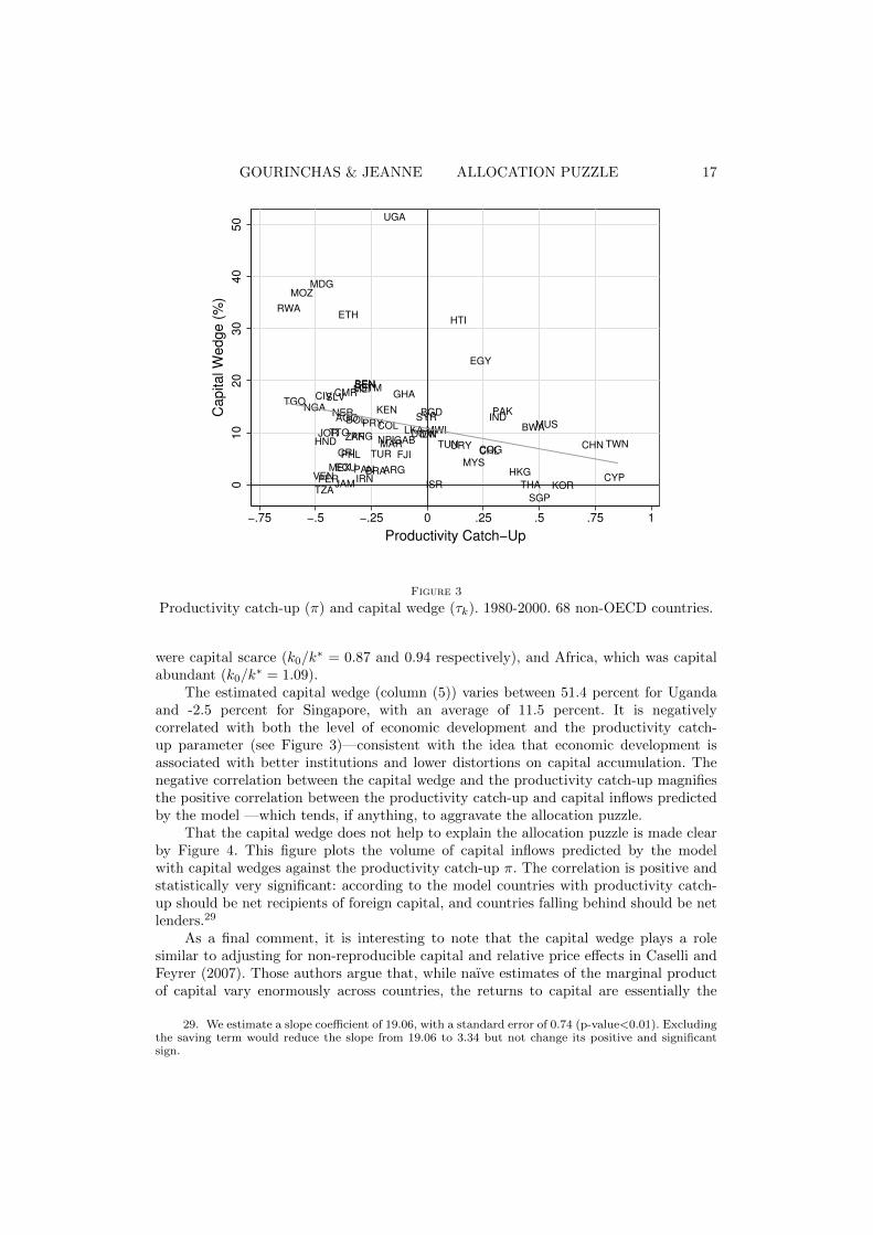
Figure 3
Productivity catch-up (π) and capital wedge (τk). 1980-2000. 68 non-OECD countries.
were capital scarce (k0/k∗ = 0.87 and 0.94 respectively), and Africa, which was capital
abundant (k0/k∗ = 1.09).
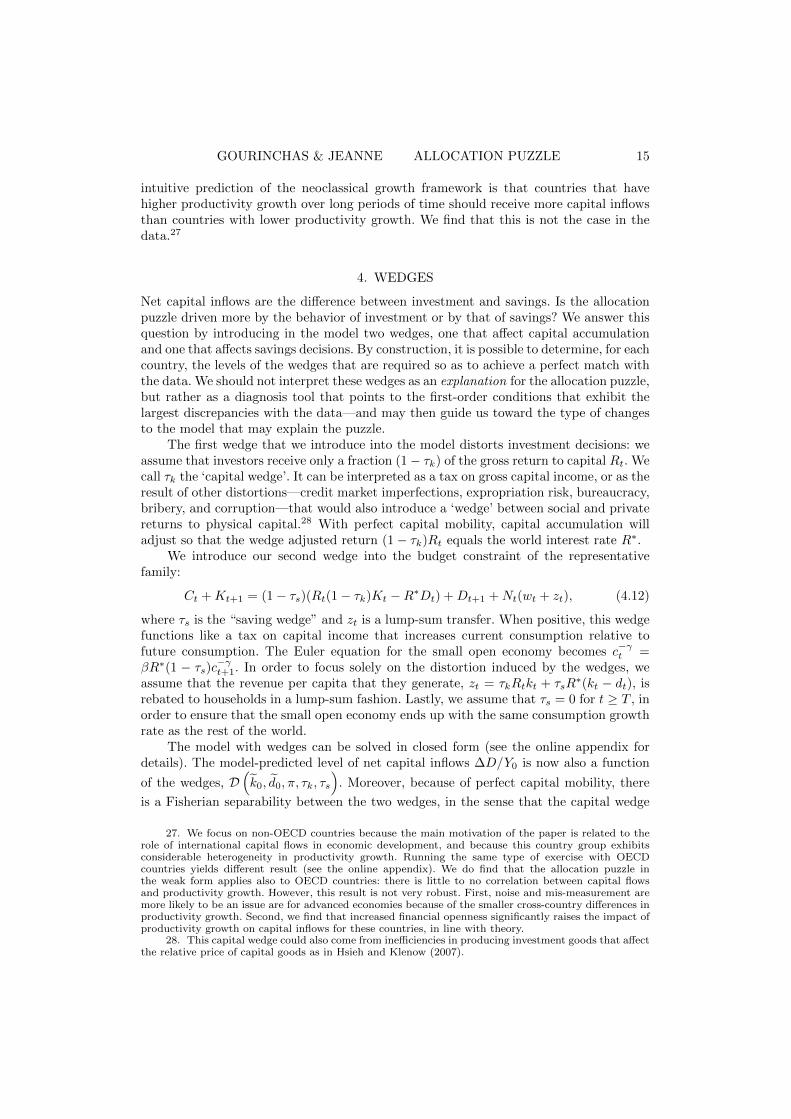
The estimated capital wedge (column (5)) varies between 51.4 percent for Ugandaand -2.5 percent for Singapore, with an average of 11.5 percent. It is negativelycorrelated with both the level of economic development and the productivity catch-up parameter (see Figure 3)—consistent with the idea that economic development isassociated with better institutions and lower distortions on capital accumulation. Thenegative correlation between the capital wedge and the productivity catch-up magnifiesthe positive correlation between the productivity catch-up and capital inflows predictedby the model —which tends, if anything, to aggravate the allocation puzzle.
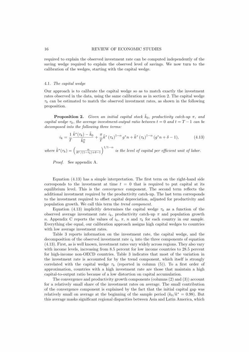
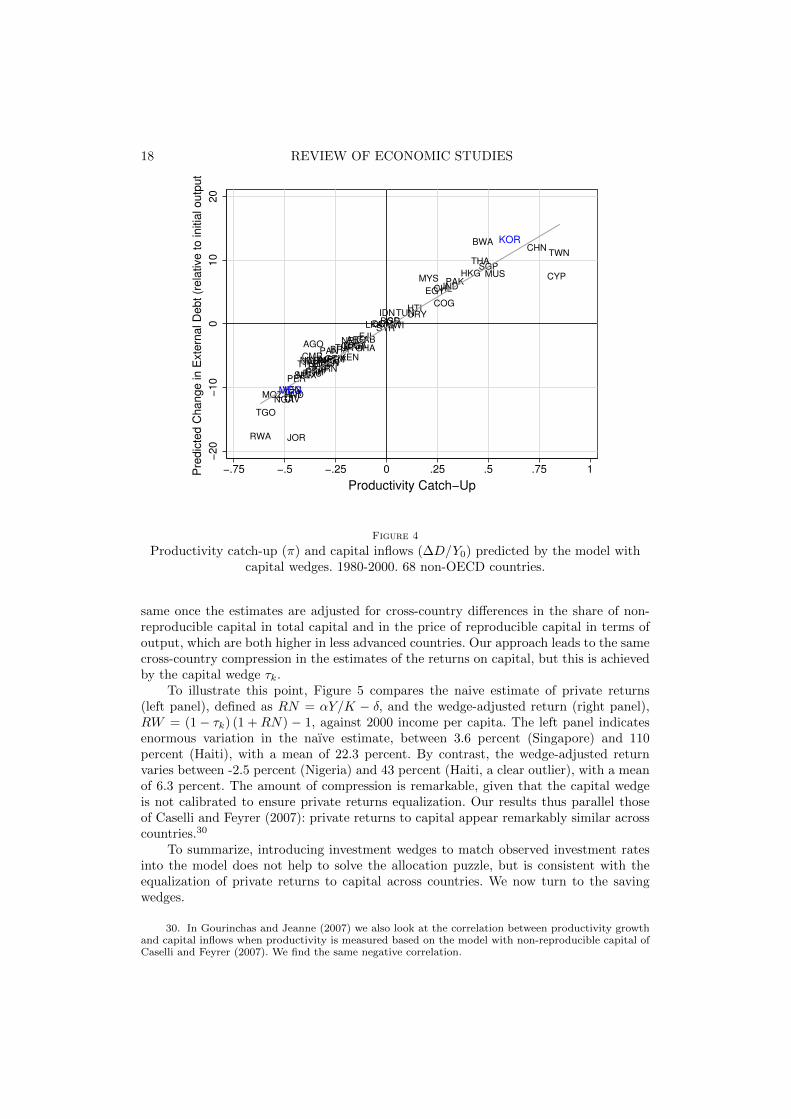
That the capital wedge does not help to explain the allocation puzzle is made clearby Figure 4. This figure plots the volume of capital inflows predicted by the modelwith capital wedges against the productivity catch-up π. The correlation is positive andstatistically very significant: according to the model countries with productivity catch-up should be net recipients of foreign capital, and countries falling behind should be netlenders.29
As a final comment, it is interesting to note that the capital wedge plays a rolesimilar to adjusting for non-reproducible capital and relative price effects in Caselli andFeyrer (2007). Those authors argue that, while naıve estimates of the marginal productof capital vary enormously across countries, the returns to capital are essentially the
29. We estimate a slope coefficient of 19.06, with a standard error of 0.74 (p-value<0.01). Excludingthe saving term would reduce the slope from 19.06 to 3.34 but not change its positive and significantsign.
18 REVIEW OF ECONOMIC STUDIES
AGO ARG
BEN
BGD
BOL
BRA
BWA
CHL
CHN
CIV
CMR
COG
COL
CRI
CYP
DOM
ECU
EGY
ETH
FJIGABGHA
GTM
HKG
HND
HTIIDN
IND
IRN
ISR
JAM
JOR
KEN
LKA
MAR
MEX
MLI
MOZ
MUS
MWI
MYS
NER
NGA
NPL
PAK
PAN
PER
PHLPNGPRY
RWA
SEN
SGP
SLV
SYR
TGO
THA
TTO
TUN
TUR
TWN
TZA
UGA
URY
VEN
ZAF
KOR
MDG
−2
0−
10
01
02
0
Pre
dic
ted
Ch
an
ge
in
Exte
rna
l D
eb
t (r
ela
tive
to
in
itia
l o
utp
ut)
−.75 −.5 −.25 0 .25 .5 .75 1
Productivity Catch−Up
Figure 4
Productivity catch-up (π) and capital inflows (∆D/Y0) predicted by the model withcapital wedges. 1980-2000. 68 non-OECD countries.
same once the estimates are adjusted for cross-country differences in the share of non-reproducible capital in total capital and in the price of reproducible capital in terms ofoutput, which are both higher in less advanced countries. Our approach leads to the samecross-country compression in the estimates of the returns on capital, but this is achievedby the capital wedge τk.
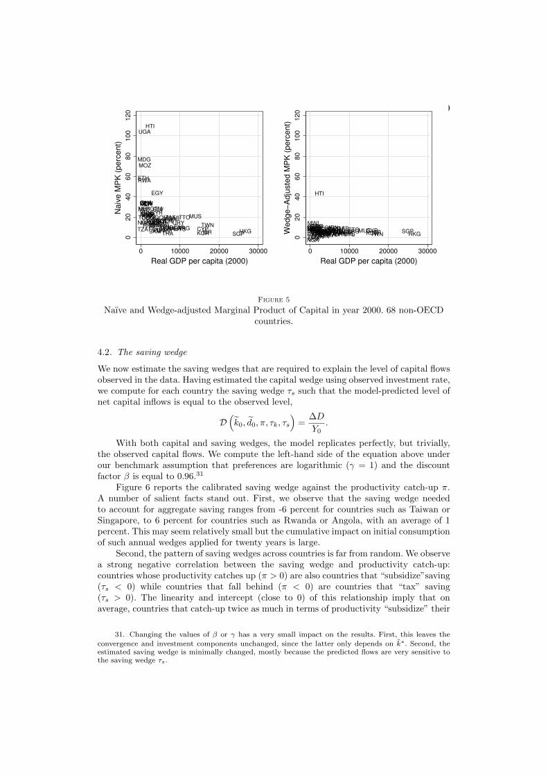
To illustrate this point, Figure 5 compares the naive estimate of private returns(left panel), defined as RN = αY/K − δ, and the wedge-adjusted return (right panel),RW = (1− τk) (1 +RN) − 1, against 2000 income per capita. The left panel indicatesenormous variation in the naıve estimate, between 3.6 percent (Singapore) and 110percent (Haiti), with a mean of 22.3 percent. By contrast, the wedge-adjusted returnvaries between -2.5 percent (Nigeria) and 43 percent (Haiti, a clear outlier), with a meanof 6.3 percent. The amount of compression is remarkable, given that the capital wedgeis not calibrated to ensure private returns equalization. Our results thus parallel thoseof Caselli and Feyrer (2007): private returns to capital appear remarkably similar acrosscountries.30
To summarize, introducing investment wedges to match observed investment ratesinto the model does not help to solve the allocation puzzle, but is consistent with theequalization of private returns to capital across countries. We now turn to the savingwedges.
30. In Gourinchas and Jeanne (2007) we also look at the correlation between productivity growthand capital inflows when productivity is measured based on the model with non-reproducible capital ofCaselli and Feyrer (2007). We find the same negative correlation.
GOURINCHAS & JEANNE ALLOCATION PUZZLE 19
AGO
ARG
BEN
BGDBOL
BRA
BWA
CHLCHN
CIV
CMRCOG COL
CRICYP
DOM
ECU
EGY
ETH
FJIGAB
GHAGTM
HKGHND
HTI
IDN
IND
IRNISRJAM
JOR
KEN
KOR
LKAMAR
MDG
MEX
MLI
MOZ
MUS
MWI
MYS
NER
NGANPL
PAK
PANPERPHL
PNGPRY
RWA
SEN
SGP
SLVSYR
TGO
THA
TTOTUNTUR TWN
TZA
UGA
URYVEN
ZAF
020
40
60
80
100
120
Naiv
e M
PK
(perc
ent)
0 10000 20000 30000
Real GDP per capita (2000)
AGO ARGBENBGDBOL BRABWACHLCHNCIV
CMR
COG
COLCRI CYPDOMECUEGY
ETH FJI GABGHAGTM HKGHND
HTI
IDNIND
IRNISRJAM
JORKEN KORLKAMAR
MDGMEX
MLIMOZ MUS
MWI
MYS
NER
NGA
NPLPAK PANPERPHLPNGPRYRWA
SEN SGPSLVSYR
TGOTHA
TTOTUNTUR TWN
TZA
UGA
URYVENZAF
020
40
60
80
100
120
Wed
ge−
Adju
ste
d M
PK
(perc
en
t)
0 10000 20000 30000
Real GDP per capita (2000)
Figure 5
Naıve and Wedge-adjusted Marginal Product of Capital in year 2000. 68 non-OECDcountries.
4.2. The saving wedge
We now estimate the saving wedges that are required to explain the level of capital flowsobserved in the data. Having estimated the capital wedge using observed investment rate,we compute for each country the saving wedge τs such that the model-predicted level ofnet capital inflows is equal to the observed level,
D(k0, d0, π, τk, τs
)=
∆D
Y0.
With both capital and saving wedges, the model replicates perfectly, but trivially,the observed capital flows. We compute the left-hand side of the equation above underour benchmark assumption that preferences are logarithmic (γ = 1) and the discountfactor β is equal to 0.96.31
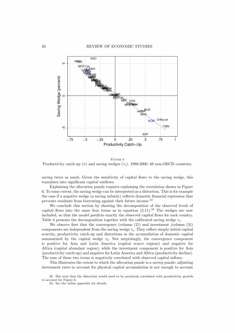
Figure 6 reports the calibrated saving wedge against the productivity catch-up π.A number of salient facts stand out. First, we observe that the saving wedge neededto account for aggregate saving ranges from -6 percent for countries such as Taiwan orSingapore, to 6 percent for countries such as Rwanda or Angola, with an average of 1percent. This may seem relatively small but the cumulative impact on initial consumptionof such annual wedges applied for twenty years is large.
Second, the pattern of saving wedges across countries is far from random. We observea strong negative correlation between the saving wedge and productivity catch-up:countries whose productivity catches up (π > 0) are also countries that “subsidize”saving(τs < 0) while countries that fall behind (π < 0) are countries that “tax” saving(τs > 0). The linearity and intercept (close to 0) of this relationship imply that onaverage, countries that catch-up twice as much in terms of productivity “subsidize” their
31. Changing the values of β or γ has a very small impact on the results. First, this leaves the
convergence and investment components unchanged, since the latter only depends on k∗. Second, theestimated saving wedge is minimally changed, mostly because the predicted flows are very sensitive tothe saving wedge τs.
20 REVIEW OF ECONOMIC STUDIES
AGO
ARG
BEN
BGD
BOL
BRA
BWA
CHL
CHN
CIV
CMR
COG
COL
CRI
CYP
DOM
ECU
EGY
ETH
FJIGABGHA
GTM
HKG
HND
HTIIDN
IND
IRN
ISR
JAMJOR
KEN
LKA
MAR
MEX
MLI
MOZ
MUS
MWI
MYS
NERNGA
NPL
PAK
PAN
PER
PHLPNG
PRY
RWA
SEN
SGP
SLV
SYR
TGO
THA
TTO
TUN
TUR
TWN
TZA
UGA
URY
VEN
ZAF
KOR
MDG
−5
05
Savin
g W
edge (
perc
ent)
−.75 −.5 −.25 0 .25 .5 .75 1
Productivity Catch−Up
Figure 6
Productivity catch-up (π) and saving wedges (τs). 1980-2000. 68 non-OECD countries.
saving twice as much. Given the sensitivity of capital flows to the saving wedge, thistranslates into significant capital outflows.
Explaining the allocation puzzle requires explaining the correlation shown in Figure6. To some extent, the saving wedge can be interpreted as a distortion. This is for examplethe case if a negative wedge (a saving subsidy) reflects domestic financial repression thatprevents residents from borrowing against their future income.32
We conclude this section by showing the decomposition of the observed levels ofcapital flows into the same four terms as in equation (2.11).33 The wedges are nowincluded, so that the model predicts exactly the observed capital flows for each country.Table 4 presents the decomposition together with the calibrated saving wedge τs.
We observe first that the convergence (column (2)) and investment (column (3))components are independent from the saving wedge τs. They reflect simply initial capitalscarcity, productivity catch-up and distortions in the accumulation of domestic capitalsummarized by the capital wedge τk. Not surprisingly, the convergence componentis positive for Asia and Latin America (capital scarce regions) and negative forAfrica (capital abundant region), while the investment component is positive for Asia(productivity catch-up) and negative for Latin America and Africa (productivity decline).The sum of these two terms is negatively correlated with observed capital inflows.
This illustrates the extent to which the allocation puzzle is a saving puzzle: adjustinginvestment rates to account for physical capital accumulation is not enough to account
32. But note that the distortion would need to be positively correlated with productivity growthto account for Figure 6.
33. See the online appendix for details.
GOURINCHAS & JEANNE ALLOCATION PUZZLE 21
for patterns of capital flows across countries. The saving wedge is essential to account forthe observed pattern of net capital flows across developing countries. Our wedge analysisindicates that Asia subsidizes saving (τs = −1.14 percent) whereas Latin America andAfrica tax savings similarly (τs = 1.83 and 1.79 percent respectively). Similarly, thesaving wedge decreases with the level of development.
5. PUBLIC VS. PRIVATE FLOWS
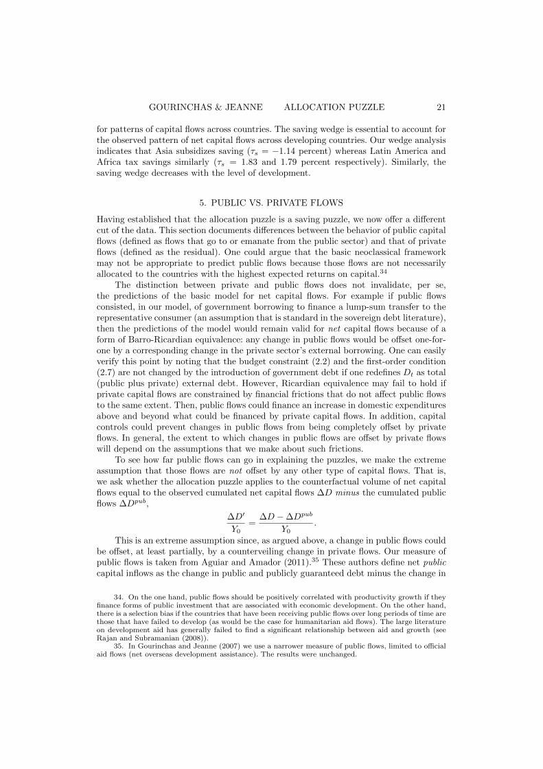
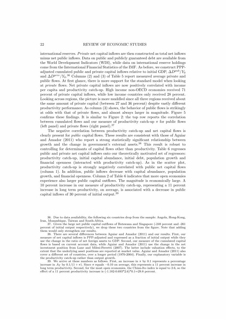
Having established that the allocation puzzle is a saving puzzle, we now offer a differentcut of the data. This section documents differences between the behavior of public capitalflows (defined as flows that go to or emanate from the public sector) and that of privateflows (defined as the residual). One could argue that the basic neoclassical frameworkmay not be appropriate to predict public flows because those flows are not necessarilyallocated to the countries with the highest expected returns on capital.34
The distinction between private and public flows does not invalidate, per se,the predictions of the basic model for net capital flows. For example if public flowsconsisted, in our model, of government borrowing to finance a lump-sum transfer to therepresentative consumer (an assumption that is standard in the sovereign debt literature),then the predictions of the model would remain valid for net capital flows because of aform of Barro-Ricardian equivalence: any change in public flows would be offset one-for-one by a corresponding change in the private sector’s external borrowing. One can easilyverify this point by noting that the budget constraint (2.2) and the first-order condition(2.7) are not changed by the introduction of government debt if one redefines Dt as total(public plus private) external debt. However, Ricardian equivalence may fail to hold ifprivate capital flows are constrained by financial frictions that do not affect public flowsto the same extent. Then, public flows could finance an increase in domestic expendituresabove and beyond what could be financed by private capital flows. In addition, capitalcontrols could prevent changes in public flows from being completely offset by privateflows. In general, the extent to which changes in public flows are offset by private flowswill depend on the assumptions that we make about such frictions.
To see how far public flows can go in explaining the puzzles, we make the extremeassumption that those flows are not offset by any other type of capital flows. That is,we ask whether the allocation puzzle applies to the counterfactual volume of net capitalflows equal to the observed cumulated net capital flows ∆D minus the cumulated publicflows ∆Dpub,
∆D′
Y0=
∆D −∆Dpub
Y0.
This is an extreme assumption since, as argued above, a change in public flows couldbe offset, at least partially, by a counterveiling change in private flows. Our measure ofpublic flows is taken from Aguiar and Amador (2011).35 These authors define net publiccapital inflows as the change in public and publicly guaranteed debt minus the change in
34. On the one hand, public flows should be positively correlated with productivity growth if theyfinance forms of public investment that are associated with economic development. On the other hand,there is a selection bias if the countries that have been receiving public flows over long periods of time arethose that have failed to develop (as would be the case for humanitarian aid flows). The large literatureon development aid has generally failed to find a significant relationship between aid and growth (seeRajan and Subramanian (2008)).
35. In Gourinchas and Jeanne (2007) we use a narrower measure of public flows, limited to officialaid flows (net overseas development assistance). The results were unchanged.
22 REVIEW OF ECONOMIC STUDIES
international reserves. Private net capital inflows are then constructed as total net inflowsminus net public inflows. Data on public and publicly guaranteed debt are available fromthe World Development Indicators (WDI), while data on international reserve holdingscome from the International Financial Statistics of the IMF. As before, we construct PPP-adjusted cumulated public and private capital inflows relative to initial GDP, ∆Dpub/Y0
and ∆Dpriv/Y0.36 Columns (2) and (3) of Table 5 report measured average private andpublic flows. At first glance, there is more support for the standard model when lookingat private flows. Net private capital inflows are now positively correlated with incomeper capita and productivity catch-up. High income non-OECD economies received 71percent of private capital inflows, while low income countries only received 28 percent.Looking across regions, the picture is more muddled since all three regions received aboutthe same amount of private capital (between 27 and 36 percent) despite vastly differentproductivity performance. As column (3) shows, the behavior of public flows is strikinglyat odds with that of private flows, and almost always larger in magnitude. Figure 5confirms these findings. It is similar to Figure 2: the top row reports the correlationbetween cumulated flows and our measure of productivity catch-up π for public flows(left panel) and private flows (right panel).37
The negative correlation between productivity catch-up and net capital flows isclearly present for public capital flows. These results are consistent with those of Aguiarand Amador (2011) who report a strong statistically significant relationship betweengrowth and the change in government’s external assets.38 This result is robust tocontrolling for determinants of capital flows other than productivity. Table 6 regressespublic and private net capital inflows onto our theoretically motivated set of regressors:productivity catch-up, initial capital abundance, initial debt, population growth andfinancial openness (interacted with productivity catch-up). As in the scatter plot,productivity catch-up is strongly negatively correlated with public net capital flows(column 1). In addition, public inflows decrease with capital abundance, populationgrowth, and financial openness. Column 2 of Table 6 indicates that more open economiesexperience also larger public capital outflows. The magnitude is economically large. A10 percent increase in our measure of productivity catch-up, representing a 11 percentincrease in long term productivity, on average, is associated with a decrease in publiccapital inflows of 30 percent of initial output.39
36. Due to data availability, the following six countries drop from the sample: Angola, Hong-Kong,Iran, Mozambique, Taiwan and South-Africa.
37. Given the large net public capital outflows of Botswana and Singapore (-248 percent and -261percent of initial output respectively), we drop these two countries from the figure. Note that addingthem would only strengthen our results.
38. There are several differences between Aguiar and Amador (2011) and our results. First, ourmeasure of net capital inflows is PPP-adjusted and expressed as a fraction of initial output while theyuse the change in the ratio of net foreign assets to GDP. Second, our measure of the cumulated capitalflows is based on current account data, while Aguiar and Amador (2011) use the change in the netinvestment position from Lane and Milesi-Ferretti (2007). The latter include valuation effects, to theextent that the underlying asset positions are reported at market value. Aguiar and Amador (2011) alsocover a different set of countries, over a longer period (1970-2004). Finally, our explanatory variable isthe productivity catch-up rather than output growth.
39. We arrive at these numbers as follows. First, an increase in π by 0.1 represents a percentageincrease in AT by 0.1/(1 + π). Since π equals −0.10 on average, this represents a 11 percent increase inlong term productivity. Second, for the most open economies, the Chinn-Ito index is equal to 2.6, so theeffect of a 11 percent productivity increase is (-1.182-0.693*2.6)*0.1=29.8 percent.
GOURINCHAS & JEANNE ALLOCATION PUZZLE 23
CHNTHA
IND
FJI
TUR LKAPNG
NPL
PHLIDN
MYS
BGD
PAK
KOR
SLV
PRYPAN
MEXJAM
PER URYVEN
ECU
DOM
HND
CRIHTI
BRA
COLARG
CHL
BOLGTM
TTOSEN
CYPMUS
CMRETH
COG
CIVTGO
TUNKEN
BENJOR
MWI
GAB
MAR SYR
MDGRWA
UGA
EGY
NERGHA
ISR
NGA
TZA
MLI
-1-.5
0.5
1Pu
blic
Capi
tal I
nflow
s (re
lativ
e to
initia
l out
put)
-0.75 -0.50 -0.25 0.00 0.25 0.50 0.75 1.00Productivity Catch-Up
(a) Net Public Capital Inflows
CHN
THA
IND
FJI
TURLKA
PNG
NPL
PHL
IDN
MYS
BGD
SGP
PAKKOR
SLV
PRY
PAN
MEX
JAM
PER
URY
VEN
ECUDOMHND
CRI
HTIBRA
COL
ARG
CHL
BOL
GTM
TTO
SENCYP
MUS
CMR
ETH
COG
CIVTGO
TUNKEN
BEN
JORMWI
GAB
MAR
SYR
BWA
MDGRWAUGA
EGY
NER
GHA
ISR
NGA
TZA
MLI
-.50
.51
1.5
Priva
te C
apita
l Infl
ows
(rela
tive
to in
itial o
utpu
t)
-0.75 -0.50 -0.25 0.00 0.25 0.50 0.75 1.00Productivity Catch-Up
(b) Net Private Capital Inflows
CHN
THA
IND
FJI
TUR
LKA
PNG
NPL
PHL
IDN
MYS
BGD
HKGSGP
PAK
KOR
SLV
PRY
PAN
MEXJAM
PER
URYVEN
ECU
DOM
HND
CRI HTI
BRA
COLARG
CHL
BOL
GTMTTO
SEN
CYP
MUS
CMR
ETH
COG
CIVTGO
TUN
KEN
BEN
JOR
MWI
GAB
MAR
SYR
BWA
MDG
RWA
UGA
IRN EGY
NER
GHA
ISR
NGA
TZA
MLI
0.2
.4.6
.8PP
G C
apita
l Infl
ows
(rela
tive
to in
itial o
utpu
t)
-0.75 -0.50 -0.25 0.00 0.25 0.50 0.75 1.00Productivity Catch-Up
(c) Net Publicly and Publicly Guaranteed CapitalInflows
CHN
THA
INDFJI
TUR
LKAPNG
NPL
PHL
IDN
MYS
BGD PAK
KOR
SLV
PRY
PANMEXJAMPERURY
VENECU
DOM
HND
CRI
HTIBRACOLARG
CHL
BOLGTM
TTO
SEN
CYP
MUS
CMRETH COG
CIVTGO TUNKEN
BEN
JOR
MWIGAB
MAR
SYRMDG
RWA
UGAEGY
NER GHA
ISR
NGA
TZA MLI
-.8-.6
-.4-.2
0.2
-Offi
cial R
eser
ve A
ccum
ulat
ion
(rela
tive
to in
itial o
utpu
t)
-0.75 -0.50 -0.25 0.00 0.25 0.50 0.75 1.00Productivity Catch-Up
(d) (opposite of) International Reserves Flows
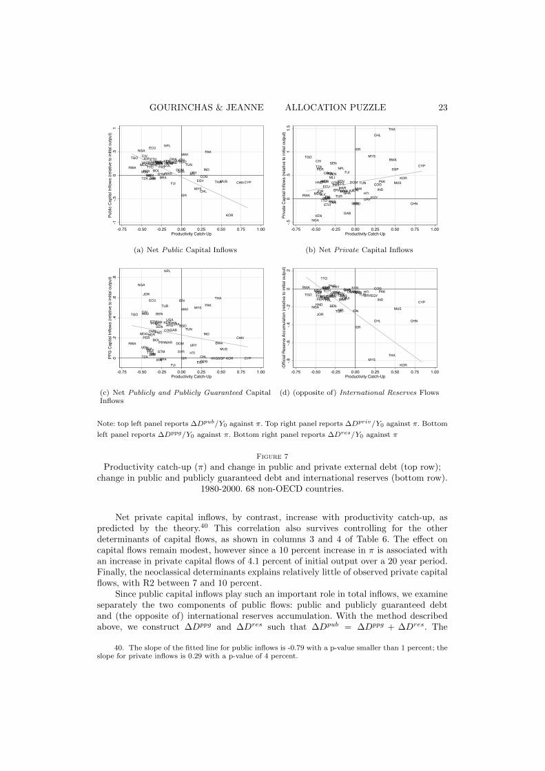
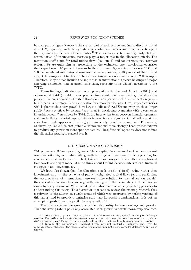
Note: top left panel reports ∆Dpub/Y0 against π. Top right panel reports ∆Dpriv/Y0 against π. Bottom
left panel reports ∆Dppg/Y0 against π. Bottom right panel reports ∆Dres/Y0 against π
Figure 7
Productivity catch-up (π) and change in public and private external debt (top row);change in public and publicly guaranteed debt and international reserves (bottom row).
1980-2000. 68 non-OECD countries.
Net private capital inflows, by contrast, increase with productivity catch-up, aspredicted by the theory.40 This correlation also survives controlling for the otherdeterminants of capital flows, as shown in columns 3 and 4 of Table 6. The effect oncapital flows remain modest, however since a 10 percent increase in π is associated withan increase in private capital flows of 4.1 percent of initial output over a 20 year period.Finally, the neoclassical determinants explains relatively little of observed private capitalflows, with R2 between 7 and 10 percent.
Since public capital inflows play such an important role in total inflows, we examineseparately the two components of public flows: public and publicly guaranteed debtand (the opposite of) international reserves accumulation. With the method describedabove, we construct ∆Dppg and ∆Dres such that ∆Dpub = ∆Dppg + ∆Dres. The
40. The slope of the fitted line for public inflows is -0.79 with a p-value smaller than 1 percent; theslope for private inflows is 0.29 with a p-value of 4 percent.
24 REVIEW OF ECONOMIC STUDIES
bottom part of figure 5 reports the scatter plot of each component (normalized by initialoutput Y0) against productivity catch-up π while columns 5 and 6 of Table 6 reportthe regression coefficients with covariates.41 The results indicate unambiguously that theaccumulation of international reserves plays a major role in the allocation puzzle. Theregression coefficients for total public flows (column 2) and for international reserves(column 6) are quite similar. According to the estimates, open developing countriesthat experience a 10 percent increase in their productivity catch-up between 1980 and2000 accumulated international reserves accounting for about 30 percent of their initialoutput. It is important to observe that these estimates are obtained on a pre-2000 sample.Therefore, they do not include the rapid rise in international reserve holdings of majoremerging economies that occurred since then, especially after China’s accession to theWTO.
These findings indicate that, as emphasized by Aguiar and Amador (2011) andAlfaro et al. (2011), public flows play an important role in explaining the allocationpuzzle. The consideration of public flows does not per se resolve the allocation puzzlebut it leads us to reformulate the question in a more precise way. First, why do countrieswith higher productivity growth have larger public outflows? Second, why are those largerpublic flows not offset by private flows, even in developing economies with a very openfinancial account? As shown by Table 2, the interaction term between financial opennessand productivity on total capital inflows is negative and significant, indicating that theallocation puzzle applies more strongly to financially more open economies. The reason,as shown by Table 6, is that public outflows respond more strongly than private inflowsto productivity growth in more open economies. Thus, financial openness does not reducethe allocation puzzle, it exacerbates it.
6. DISCUSSION AND CONCLUSION
This paper establishes a puzzling stylized fact: capital does not tend to flow more towardcountries with higher productivity growth and higher investment. This is puzzling forneoclassical models of growth—in fact, this makes one wonder if the textbook neoclassicalframework is the right model at all to think about the link between international financialintegration and development.
We have also shown that the allocation puzzle is related to (i) saving rather thaninvestment, and (ii) the behavior of publicly originated capital flows (and in particular,the accumulation of international reserves). The solution to the “allocation puzzle”thus lies at the nexus of between growth, saving and the accumulation of net foreignassets by the government. We conclude with a discussion of some possible approaches tounderstanding this nexus. This discussion is meant to review the existing research thatis relevant to the allocation puzzle (some of which was motivated by earlier versions ofthis paper) and to provide a tentative road map for possible explanations. It is not anattempt to push forward a particular explanation.42
The first angle on the question is the relationship between savings and growth.That the saving rate is positively associated with growth is a well-known empirical fact.
41. As for the top panels of figure 5, we exclude Botswana and Singapore from the plot of foreignreserves. Our estimates indicate that reserve accumulation for these two countries amounted to about-260 percent of their 1980 output. Once again, adding them back would only strengthen our results.
42. Indeed, the explanations reviewed below are not mutually exclusive, and may becomplementary. Moreover, the most relevant explanation may not be the same for different countries orregions.
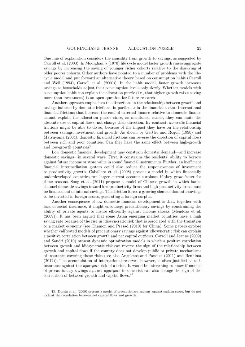
GOURINCHAS & JEANNE ALLOCATION PUZZLE 25
One line of explanation considers the causality from growth to savings, as suggested byCarroll et al. (2000). In Modigliani’s (1970) life cycle model faster growth raises aggregatesavings by increasing the saving of younger richer cohorts relative to the dissaving ofolder poorer cohorts. Other authors have pointed to a number of problems with the life-cycle model and put forward an alternative theory based on consumption habit (Carrolland Weil (1994), Carroll et al. (2000)). In the habit model, faster growth increasessavings as households adjust their consumption levels only slowly. Whether models withconsumption habit can explain the allocation puzzle (i.e., that higher growth raises savingmore than investment) is an open question for future research.
Another approach emphasizes the distortions in the relationship between growth andsavings induced by domestic frictions, in particular in the financial sector. Internationalfinancial frictions that increase the cost of external finance relative to domestic financecannot explain the allocation puzzle since, as mentioned earlier, they can mute theabsolute size of capital flows, not change their direction. By contrast, domestic financialfrictions might be able to do so, because of the impact they have on the relationshipbetween savings, investment and growth. As shown by Gertler and Rogoff (1990) andMatsuyama (2004), domestic financial frictions can reverse the direction of capital flowsbetween rich and poor countries. Can they have the same effect between high-growthand low-growth countries?
Low domestic financial development may constrain domestic demand—and increasedomestic savings—in several ways. First, it constrains the residents’ ability to borrowagainst future income or store value in sound financial instruments. Further, an inefficientfinancial intermediation system could also reduce the responsiveness of investmentto productivity growth. Caballero et al. (2008) present a model in which financiallyunderdeveloped countries run larger current account surpluses if they grow faster forthese reasons. Song et al. (2011) propose a model of Chinese growth in which bankschannel domestic savings toward low-productivity firms and high-productivity firms mustbe financed out of internal savings. This friction forces a growing share of domestic savingsto be invested in foreign assets, generating a foreign surplus.
Another consequence of low domestic financial development is that, together withlack of social insurance, it might encourage precautionary savings by constraining theability of private agents to insure efficiently against income shocks (Mendoza et al.(2009)). It has been argued that some Asian emerging market countries have a highsaving rate because of the rise in idiosyncratic risk that is associated with the transitionto a market economy (see Chamon and Prasad (2010) for China). Some papers explorewhether calibrated models of precautionary savings against idiosyncratic risk can explaina positive correlation between growth and net capital outflows. Carroll and Jeanne (2009)and Sandri (2010) present dynamic optimization models in which a positive correlationbetween growth and idiosyncratic risk can reverse the sign of the relationship betweengrowth and capital flows if the country does not develop public or private mechanismsof insurance covering those risks (see also Angeletos and Panousi (2011) and Benhima(2012)). The accumulation of international reserves, however, is often justified as self-insurance against the aggregate risk of a crisis. It would be interesting to know if modelsof precautionary savings against aggregate income risk can also change the sign of thecorrelation of between growth and capital flows.43
43. Durdu et al. (2009) present a model of precautionary savings against sudden stops, but do notlook at the correlation between net capital flows and growth.

26 REVIEW OF ECONOMIC STUDIES
Causality could also run in the opposite direction, from savings to growth. This isthe case in many closed-economy models of endogenous growth, but this feature does noteasily survive perfect capital mobility, which makes domestic savings a small componentof the global savings pool. For domestic savings to increase growth in the open economy,there must be a friction that prevents domestic savings and foreign savings from beingperfect substitutes. Aghion et al. (2006) present an example of a model with thosefeatures.44
One common feature—and a limitation—of the models discussed above is that theydo not give a meaningful and distinct role to the government, and thus do not speak tothe fact that the allocation puzzle seems to reflect the behavior of public capital flows.The only way that these models can incorporate that fact is by claiming that the public orprivate nature of the flows is inessential: that the international reserves accumulated bythe government, for example, corresponds to a stock of foreign wealth that the privatesector wishes to accumulate anyway. We now turn to lines of explanations in whichgovernment policies are instead central to the allocation puzzle.
One line of explanation is related to the “Bretton Woods 2” view of the internationalmonetary system developed by Dooley et al. (2004a). This view has not received a full-fledged theoretical treatment but could be applied to the allocation puzzle as follows.Countries with a take-off in their tradable sector (such as China) tend to resist the realappreciation of their currency through various policies, most notably the accumulationof foreign assets by the public sector combined with restrictions on capital inflows.45 Theallocation puzzle, thus, would come from the fact that developing countries with highergrowth in the tradable sector would tend to have higher trade surpluses and so (as amatter of accounting) larger net capital outflows.
In addition, Dooley et al. (2004b) surmise that the accumulation of internationalreserves can also be interpreted as a form of collateral for the FDI flows to China.This point is formalized by Aguiar and Amador (2011) in the context of a model withan interaction between political economy and contracting frictions. In their model, thedomestic government has limited commitment so that foreign investors fear expropriation(on their capital holdings) and default (on their sovereign debt holdings). In the self-enforcing equilibrium of the model, growth requires that governments pay down theirdebt, thus reducing their external liabilities. Their model generates, along the transitionpath of a developing economy, the negative correlation between net public capital inflowsand growth that we document in this paper.
These contributions are interesting but rely, implicitly or explicitly, on theassumption that the government can control the volume of net capital flows. This isnot true in the frictionless neoclassical model, because the accumulation of reservesby the government should be offset one-for-one by higher capital inflows. This mustbe prevented by frictions, either natural (low financial development) or policy-induced(capital controls). In Aguiar and Amador (2011), for example, the domestic voters haveno access to international capital markets. The question, then, is how to reconcile thisline of explanation with our finding that the allocation puzzle is in fact stronger for thecountries that are financially more integrated.
44. In their model domestic savings matters for innovation because it fosters the involvement ofdomestic intermediaries with a superior monitoring technology. However, the model does not includeinvestment in productive physical capital, and thus does not provide a realistic framework to study theallocation puzzle.
45. In addition, causality could run from real undervaluation to growth, as argued by Rodrik (2008).

GOURINCHAS & JEANNE ALLOCATION PUZZLE 27
To conclude, there is no shortage of candidates but the main explanation(s) for theallocation puzzle remains in our view an open question. It seems important to know moreabout the underlying cause of this puzzle if one wants to understand how internationalfinancial integration helps economic development.
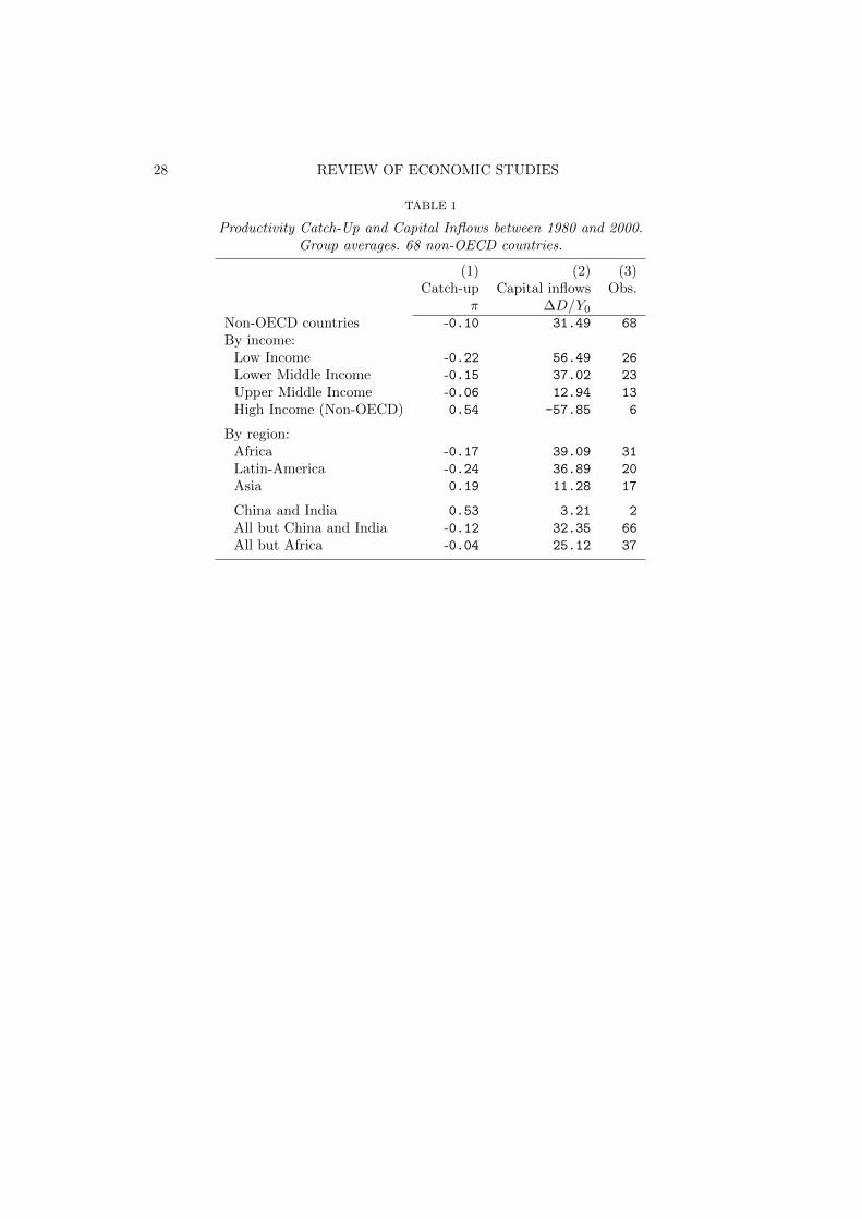
28 REVIEW OF ECONOMIC STUDIES
TABLE 1
Productivity Catch-Up and Capital Inflows between 1980 and 2000.Group averages. 68 non-OECD countries.
(1) (2) (3)Catch-up Capital inflows Obs.
π ∆D/Y0
Non-OECD countries -0.10 31.49 68
By income:Low Income -0.22 56.49 26
Lower Middle Income -0.15 37.02 23
Upper Middle Income -0.06 12.94 13
High Income (Non-OECD) 0.54 -57.85 6
By region:Africa -0.17 39.09 31
Latin-America -0.24 36.89 20
Asia 0.19 11.28 17
China and India 0.53 3.21 2
All but China and India -0.12 32.35 66
All but Africa -0.04 25.12 37
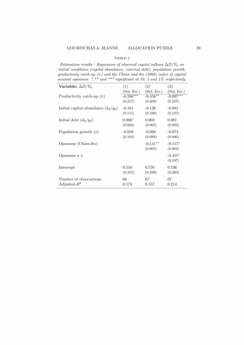
GOURINCHAS & JEANNE ALLOCATION PUZZLE 29
TABLE 2
Estimation results : Regression of observed capital inflows ∆D/Y0 oninitial conditions (capital abundance, external debt), population growth,productivity catch-up (π) and the Chinn and Ito (2008) index of capitalaccount openness. *,** and *** significant at 10, 5 and 1% respectively.
Variable: ∆D/Y0 (1) (2) (3)(Std. Err.) (Std. Err.) (Std. Err.)
Productivity catch-up (π) -0.586∗∗∗ -0.456∗∗ -0.697∗∗∗
(0.217) (0.209) (0.227)
Initial capital abundance (k0/y0) -0.161 -0.126 -0.081(0.115) (0.109) (0.107)
Initial debt (d0/y0) 0.006∗ 0.004 0.001(0.003) (0.003) (0.003)
Population growth (n) -0.058 -0.098 -0.073(0.104) (0.099) (0.096)
Openness (Chinn-Ito) -0.141∗∗ -0.115∗
(0.063) (0.062)
Openness x π -0.455∗
(0.197)
Intercept 0.516 0.576 0.536(0.315) (0.299) (0.289)
Number of observations 68 67 67Adjusted-R2 0.174 0.157 0.214
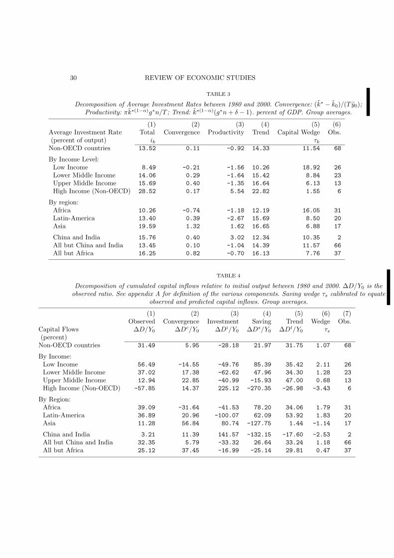
30 REVIEW OF ECONOMIC STUDIES
TABLE 3
Decomposition of Average Investment Rates between 1980 and 2000. Convergence: (k∗ − k0)/(T y0);Productivity: πk∗(1−α)g∗n/T ; Trend: k∗(1−α)(g∗n+ δ − 1). percent of GDP. Group averages.
(1) (2) (3) (4) (5) (6)Average Investment Rate Total Convergence Productivity Trend Capital Wedge Obs.(percent of output) ik τk
Non-OECD countries 13.52 0.11 -0.92 14.33 11.54 68
By Income Level:Low Income 8.49 -0.21 -1.56 10.26 18.92 26
Lower Middle Income 14.06 0.29 -1.64 15.42 8.84 23
Upper Middle Income 15.69 0.40 -1.35 16.64 6.13 13
High Income (Non-OECD) 28.52 0.17 5.54 22.82 1.55 6
By region:Africa 10.26 -0.74 -1.18 12.19 16.05 31
Latin-America 13.40 0.39 -2.67 15.69 8.50 20
Asia 19.59 1.32 1.62 16.65 6.88 17
China and India 15.76 0.40 3.02 12.34 10.35 2
All but China and India 13.45 0.10 -1.04 14.39 11.57 66
All but Africa 16.25 0.82 -0.70 16.13 7.76 37
TABLE 4
Decomposition of cumulated capital inflows relative to initial output between 1980 and 2000. ∆D/Y0 is theobserved ratio. See appendix A for definition of the various components. Saving wedge τs calibrated to equate
observed and predicted capital inflows. Group averages.
(1) (2) (3) (4) (5) (6) (7)Observed Convergence Investment Saving Trend Wedge Obs.
Capital Flows ∆D/Y0 ∆Dc/Y0 ∆Di/Y0 ∆Ds/Y0 ∆Dt/Y0 τs(percent)
Non-OECD countries 31.49 5.95 -28.18 21.97 31.75 1.07 68
By Income:Low Income 56.49 -14.55 -49.76 85.39 35.42 2.11 26
Lower Middle Income 37.02 17.38 -62.62 47.96 34.30 1.28 23
Upper Middle Income 12.94 22.85 -40.99 -15.93 47.00 0.68 13
High Income (Non-OECD) -57.85 14.37 225.12 -270.35 -26.98 -3.43 6
By Region:Africa 39.09 -31.64 -41.53 78.20 34.06 1.79 31
Latin-America 36.89 20.96 -100.07 62.09 53.92 1.83 20
Asia 11.28 56.84 80.74 -127.75 1.44 -1.14 17
China and India 3.21 11.39 141.57 -132.15 -17.60 -2.53 2
All but China and India 32.35 5.79 -33.32 26.64 33.24 1.18 66
All but Africa 25.12 37.45 -16.99 -25.14 29.81 0.47 37
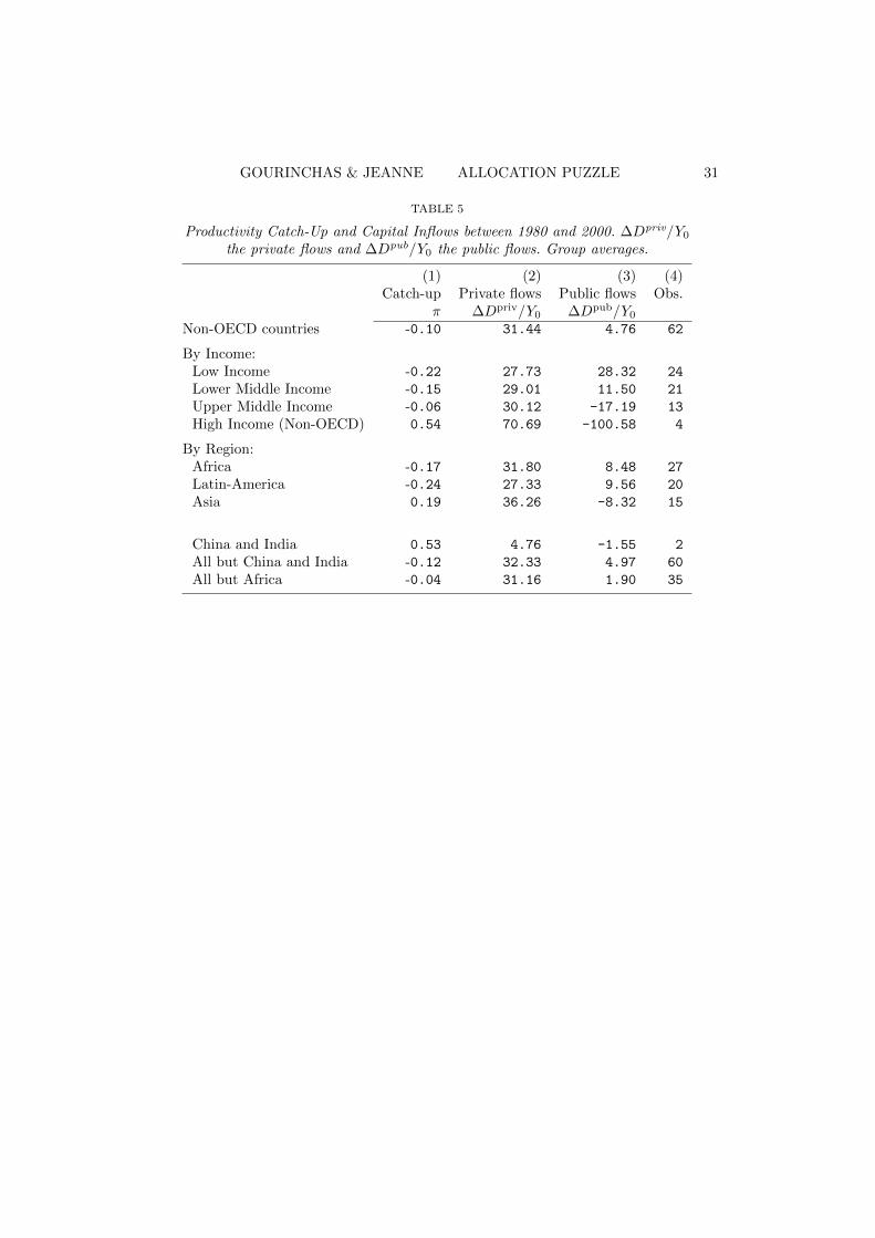
GOURINCHAS & JEANNE ALLOCATION PUZZLE 31
TABLE 5
Productivity Catch-Up and Capital Inflows between 1980 and 2000. ∆Dpriv/Y0
the private flows and ∆Dpub/Y0 the public flows. Group averages.
(1) (2) (3) (4)Catch-up Private flows Public flows Obs.
π ∆Dpriv/Y0 ∆Dpub/Y0
Non-OECD countries -0.10 31.44 4.76 62
By Income:Low Income -0.22 27.73 28.32 24
Lower Middle Income -0.15 29.01 11.50 21
Upper Middle Income -0.06 30.12 -17.19 13
High Income (Non-OECD) 0.54 70.69 -100.58 4
By Region:Africa -0.17 31.80 8.48 27
Latin-America -0.24 27.33 9.56 20
Asia 0.19 36.26 -8.32 15
China and India 0.53 4.76 -1.55 2
All but China and India -0.12 32.33 4.97 60
All but Africa -0.04 31.16 1.90 35
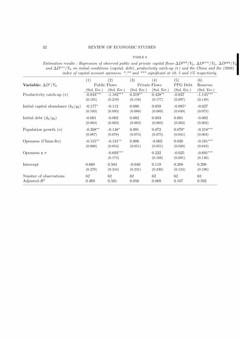
32 REVIEW OF ECONOMIC STUDIES
TABLE 6
Estimation results : Regression of observed public and private capital flows ∆Dpub/Y0, ∆Dpriv/Y0, ∆Dppg/Y0
and ∆Dres/Y0 on initial conditions (capital, debt), productivity catch-up (π) and the Chinn and Ito (2008)index of capital account openness. *,** and *** significant at 10, 5 and 1% respectively.
(1) (2) (3) (4) (5) (6)Variable: ∆Di/Y0 Public Flows Private Flows PPG Debt Reserves
(Std. Err.) (Std. Err.) (Std. Err.) (Std. Err.) (Std. Err.) (Std. Err.)
Productivity catch-up (π) -0.843∗∗∗ -1.182∗∗∗ 0.319∗∗ 0.428∗∗ -0.037 -1.145∗∗∗
(0.185) (0.219) (0.158) (0.177) (0.097) (0.149)
Initial capital abundance (k0/y0) -0.177∗ -0.112 0.080 0.059 -0.085∗ -0.027(0.103) (0.093) (0.088) (0.089) (0.049) (0.075)
Initial debt (d0/y0) -0.001 -0.002 0.002 0.003 0.001 -0.002(0.003) (0.003) (0.003) (0.003) (0.002) (0.002)
Population growth (n) -0.208∗∗ -0.148∗ 0.091 0.072 0.070∗ -0.218∗∗∗
(0.087) (0.078) (0.074) (0.075) (0.041) (0.063)
Openness (Chinn-Ito) -0.155∗∗ -0.131∗∗ 0.006 -0.002 0.030 -0.161∗∗∗
(0.060) (0.054) (0.051) (0.051) (0.028) (0.043)
Openness x π -0.693∗∗∗ 0.222 -0.025 -0.691∗∗∗
(0.174) (0.166) (0.091) (0.140)
Intercept 0.668 0.504 -0.040 0.119 0.208 0.298(0.270) (0.244) (0.231) (0.230) (0.124) (0.196)
Number of observations 62 62 62 62 62 62Adjusted-R2 0.369 0.501 0.056 0.069 0.107 0.592
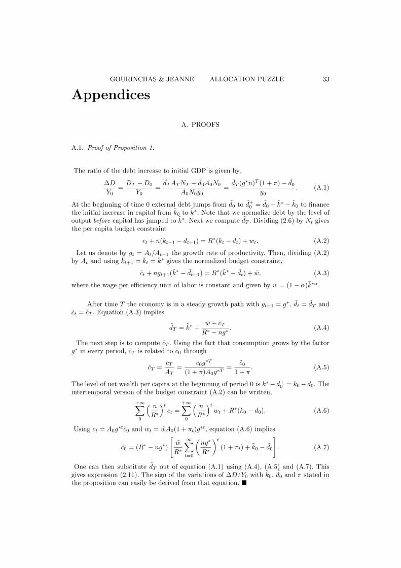
GOURINCHAS & JEANNE ALLOCATION PUZZLE 33
Appendices
A. PROOFS
A.1. Proof of Proposition 1.
The ratio of the debt increase to initial GDP is given by,
∆D
Y0=DT −D0
Y0=dTATNT − d0A0N0
A0N0y0=dT (g∗n)T (1 + π)− d0
y0. (A.1)
At the beginning of time 0 external debt jumps from d0 to d+0 = d0 + k∗ − k0 to finance
the initial increase in capital from k0 to k∗. Note that we normalize debt by the level ofoutput before capital has jumped to k∗. Next we compute dT . Dividing (2.6) by Nt givesthe per capita budget constraint
ct + n(kt+1 − dt+1) = R∗(kt − dt) + wt. (A.2)
Let us denote by gt = At/At−1 the growth rate of productivity. Then, dividing (A.2)by At and using kt+1 = kt = k∗ gives the normalized budget constraint,
ct + ngt+1(k∗ − dt+1) = R∗(k∗ − dt) + w, (A.3)
where the wage per efficiency unit of labor is constant and given by w = (1− α)k∗α.
After time T the economy is in a steady growth path with gt+1 = g∗, dt = dT andct = cT . Equation (A.3) implies
dT = k∗ +w − cTR∗ − ng∗
. (A.4)
The next step is to compute cT . Using the fact that consumption grows by the factorg∗ in every period, cT is related to c0 through
cT =cTAT
=c0g∗T
(1 + π)A0g∗T=
c01 + π
. (A.5)
The level of net wealth per capita at the beginning of period 0 is k∗− d+0 = k0− d0. The
intertemporal version of the budget constraint (A.2) can be written,
+∞∑0
( n
R∗
)tct =
+∞∑0
( n
R∗
)twt +R∗(k0 − d0). (A.6)
Using ct = A0g∗tc0 and wt = wA0(1 + πt)g
∗t, equation (A.6) implies
c0 = (R∗ − ng∗)
[w
R∗
∞∑t=0
(ng∗
R∗
)t(1 + πt) + k0 − d0
]. (A.7)
One can then substitute dT out of equation (A.1) using (A.4), (A.5) and (A.7). Thisgives expression (2.11). The sign of the variations of ∆D/Y0 with k0, d0 and π stated inthe proposition can easily be derived from that equation. �
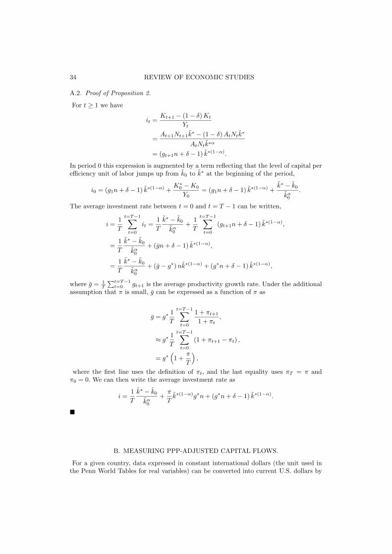
34 REVIEW OF ECONOMIC STUDIES
A.2. Proof of Proposition 2.
For t ≥ 1 we have
it =Kt+1 − (1− δ)Kt
Yt
=At+1Nt+1k
∗ − (1− δ)AtNtk∗
AtNtk∗α
= (gt+1n+ δ − 1) k∗(1−α).
In period 0 this expression is augmented by a term reflecting that the level of capital perefficiency unit of labor jumps up from k0 to k∗ at the beginning of the period,
i0 = (g1n+ δ − 1) k∗(1−α) +K∗0 −K0
Y0= (g1n+ δ − 1) k∗(1−α) +
k∗ − k0
kα0.
The average investment rate between t = 0 and t = T − 1 can be written,
i =1
T
t=T−1∑t=0
it =1
T
k∗ − k0
kα0+
1
T
t=T−1∑t=0
(gt+1n+ δ − 1) k∗(1−α),
=1
T
k∗ − k0
kα0+ (gn+ δ − 1) k∗(1−α),
=1
T
k∗ − k0
kα0+ (g − g∗)nk∗(1−α) + (g∗n+ δ − 1) k∗(1−α),
where g = 1T
∑t=T−1t=0 gt+1 is the average productivity growth rate. Under the additional
assumption that π is small, g can be expressed as a function of π as
g = g∗1
T
t=T−1∑t=0
1 + πt+1
1 + πt,
≈ g∗ 1
T
t=T−1∑t=0
(1 + πt+1 − πt) ,
= g∗(
1 +π
T
),
where the first line uses the definition of πt, and the last equality uses πT = π andπ0 = 0. We can then write the average investment rate as
i =1
T
k∗ − k0
kα0+π
Tk∗(1−α)g∗n+ (g∗n+ δ − 1) k∗(1−α).
�
B. MEASURING PPP-ADJUSTED CAPITAL FLOWS.
For a given country, data expressed in constant international dollars (the unit used inthe Penn World Tables for real variables) can be converted into current U.S. dollars by
GOURINCHAS & JEANNE ALLOCATION PUZZLE 35
multiplying them by the deflator,
Qt = PtCGDPtRGDPt
,
where CGDPt (RGDPt) is domestic GDP expressed in current (constant) internationaldollar and Pt is a price deflator. The ratio CGDP/RGDP operates the conversionfrom constant international dollar into current international dollar, and P operatesthe conversion from current international dollar into current U.S. dollar. We define thedeflator P as the price of investment goods reported in the Penn World Tables, for reasonsexplained in section 3. Multiplying a variable in constant international dollar, X, by thedeflator Q gives its value in terms of current U.S. dollars, X$ = QX.
The deflator Q can be used to obtain PPP-adjusted estimates of the observedcumulated capital inflows ∆D. To do this, we start from the external accumulationequation (in current US dollars): D$
T = D$0 −
∑T−1t=0 CA$
t ,46 and use the formulas
DT = D$T /QT and D0 = D$
0/Q0 to obtain:
∆D =
(1
QT− 1
Q0
)D$
0 −T−1∑t=0
CA$t
QT. (B.1)
The estimate of the initial net external debt in U.S. dollar (D$0) is obtained from
Lane and Milesi-Ferretti (2007)’s External Wealth of Nations Mark II database (EWN),as the difference between (the opposite of) the reported net international investmentposition (NIIP) and the errors and omissions (EO) cumulated between 1970 and 1980.47
The same approach is used to construct estimates of the initial debt output ratio d0/y0,which we need to compute the right-hand-side of (2.11).
46. Alternatively, one could use Lane and Milesi-Ferretti (2007)’s estimate of the net externalposition in year 2000. The difference between the two estimates lies in the treatment of valuation effectsdue to asset price and currency movements. The size and relative importance of these valuation effectshas increased over time. We do not attempt to incorporate these effects in this paper.
47. In keeping with usual practice, we interpret errors and omissions as unreported capital inflows.
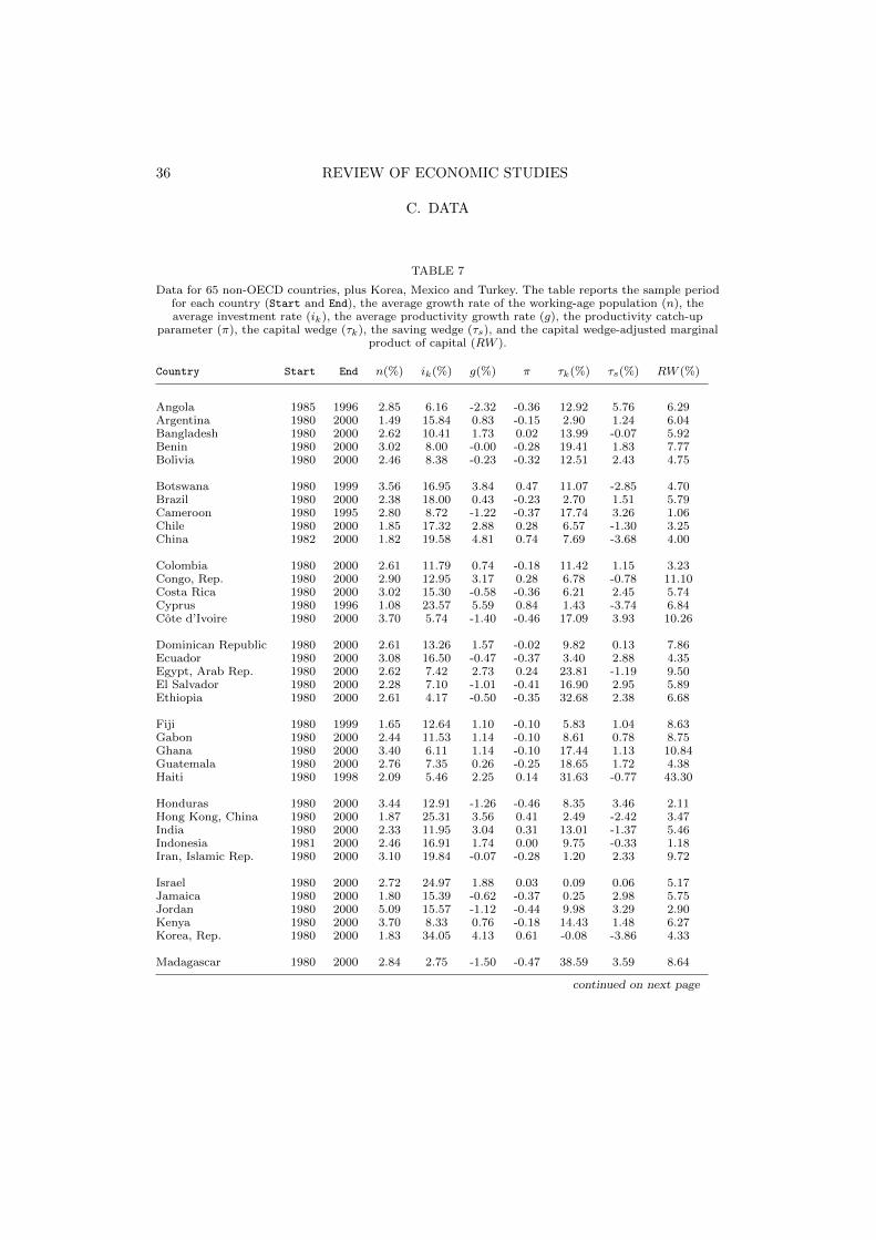
36 REVIEW OF ECONOMIC STUDIES
C. DATA
TABLE 7
Data for 65 non-OECD countries, plus Korea, Mexico and Turkey. The table reports the sample periodfor each country (Start and End), the average growth rate of the working-age population (n), theaverage investment rate (ik), the average productivity growth rate (g), the productivity catch-up
parameter (π), the capital wedge (τk), the saving wedge (τs), and the capital wedge-adjusted marginalproduct of capital (RW ).
Country Start End n(%) ik(%) g(%) π τk(%) τs(%) RW (%)
Angola 1985 1996 2.85 6.16 -2.32 -0.36 12.92 5.76 6.29Argentina 1980 2000 1.49 15.84 0.83 -0.15 2.90 1.24 6.04Bangladesh 1980 2000 2.62 10.41 1.73 0.02 13.99 -0.07 5.92Benin 1980 2000 3.02 8.00 -0.00 -0.28 19.41 1.83 7.77Bolivia 1980 2000 2.46 8.38 -0.23 -0.32 12.51 2.43 4.75
Botswana 1980 1999 3.56 16.95 3.84 0.47 11.07 -2.85 4.70Brazil 1980 2000 2.38 18.00 0.43 -0.23 2.70 1.51 5.79Cameroon 1980 1995 2.80 8.72 -1.22 -0.37 17.74 3.26 1.06Chile 1980 2000 1.85 17.32 2.88 0.28 6.57 -1.30 3.25China 1982 2000 1.82 19.58 4.81 0.74 7.69 -3.68 4.00
Colombia 1980 2000 2.61 11.79 0.74 -0.18 11.42 1.15 3.23Congo, Rep. 1980 2000 2.90 12.95 3.17 0.28 6.78 -0.78 11.10Costa Rica 1980 2000 3.02 15.30 -0.58 -0.36 6.21 2.45 5.74Cyprus 1980 1996 1.08 23.57 5.59 0.84 1.43 -3.74 6.84Cote d’Ivoire 1980 2000 3.70 5.74 -1.40 -0.46 17.09 3.93 10.26
Dominican Republic 1980 2000 2.61 13.26 1.57 -0.02 9.82 0.13 7.86Ecuador 1980 2000 3.08 16.50 -0.47 -0.37 3.40 2.88 4.35Egypt, Arab Rep. 1980 2000 2.62 7.42 2.73 0.24 23.81 -1.19 9.50El Salvador 1980 2000 2.28 7.10 -1.01 -0.41 16.90 2.95 5.89Ethiopia 1980 2000 2.61 4.17 -0.50 -0.35 32.68 2.38 6.68
Fiji 1980 1999 1.65 12.64 1.10 -0.10 5.83 1.04 8.63Gabon 1980 2000 2.44 11.53 1.14 -0.10 8.61 0.78 8.75Ghana 1980 2000 3.40 6.11 1.14 -0.10 17.44 1.13 10.84Guatemala 1980 2000 2.76 7.35 0.26 -0.25 18.65 1.72 4.38Haiti 1980 1998 2.09 5.46 2.25 0.14 31.63 -0.77 43.30
Honduras 1980 2000 3.44 12.91 -1.26 -0.46 8.35 3.46 2.11Hong Kong, China 1980 2000 1.87 25.31 3.56 0.41 2.49 -2.42 3.47India 1980 2000 2.33 11.95 3.04 0.31 13.01 -1.37 5.46Indonesia 1981 2000 2.46 16.91 1.74 0.00 9.75 -0.33 1.18Iran, Islamic Rep. 1980 2000 3.10 19.84 -0.07 -0.28 1.20 2.33 9.72
Israel 1980 2000 2.72 24.97 1.88 0.03 0.09 0.06 5.17Jamaica 1980 2000 1.80 15.39 -0.62 -0.37 0.25 2.98 5.75Jordan 1980 2000 5.09 15.57 -1.12 -0.44 9.98 3.29 2.90Kenya 1980 2000 3.70 8.33 0.76 -0.18 14.43 1.48 6.27Korea, Rep. 1980 2000 1.83 34.05 4.13 0.61 -0.08 -3.86 4.33
Madagascar 1980 2000 2.84 2.75 -1.50 -0.47 38.59 3.59 8.64
continued on next page
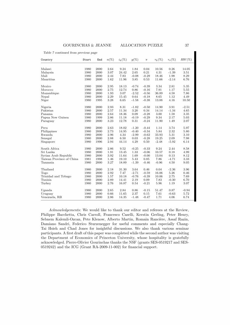
GOURINCHAS & JEANNE ALLOCATION PUZZLE 37
Table 7 continued from previous page
Country Start End n(%) ik(%) g(%) π τk(%) τs(%) RW (%)
Malawi 1980 2000 2.64 9.24 1.84 0.04 10.56 0.26 14.05Malaysia 1980 2000 3.07 24.42 2.65 0.21 4.31 -1.39 3.51Mali 1980 2000 2.44 7.83 -0.08 -0.29 18.46 1.98 8.29Mauritius 1980 2000 1.62 11.96 3.85 0.53 11.66 -2.14 6.76
Mexico 1980 2000 2.95 18.13 -0.74 -0.39 3.34 2.81 5.35Morocco 1980 2000 2.75 12.74 0.86 -0.16 7.91 1.17 5.55Mozambique 1980 2000 1.93 3.07 -2.52 -0.56 36.89 4.58 7.86Nepal 1980 2000 2.29 15.45 0.64 -0.18 8.65 1.12 4.49Niger 1980 1995 3.28 6.65 -1.58 -0.38 13.88 4.16 10.50
Nigeria 1980 2000 2.93 8.31 -1.82 -0.50 14.90 3.91 -2.51Pakistan 1980 2000 2.57 11.34 3.20 0.34 14.14 -1.34 4.65Panama 1980 2000 2.64 18.36 0.09 -0.28 3.00 1.58 3.35Papua New Guinea 1980 1999 2.86 11.18 -0.19 -0.29 9.34 2.17 5.03Paraguay 1980 2000 3.23 12.78 0.31 -0.24 11.90 1.49 2.07
Peru 1980 2000 2.63 18.02 -1.20 -0.44 1.14 3.74 5.97Philippines 1980 2000 2.73 14.95 -0.40 -0.34 5.84 2.32 5.80Rwanda 1980 2000 2.96 4.34 -2.99 -0.62 33.93 5.31 3.10Senegal 1980 2000 2.88 6.50 0.03 -0.28 19.25 2.09 7.98Singapore 1980 1996 2.94 44.14 4.29 0.50 -2.48 -5.92 6.14
South Africa 1980 2000 2.86 9.52 -0.25 -0.33 9.24 2.44 8.58Sri Lanka 1980 2000 1.91 13.45 1.33 -0.06 10.57 0.18 4.99Syrian Arab Republic 1980 2000 3.92 11.64 1.69 -0.00 13.04 0.13 8.12Taiwan Province of China 1981 1998 1.46 19.10 5.43 0.85 7.86 -4.71 3.33Tanzania 1980 2000 3.27 18.89 -1.39 -0.46 -0.96 4.50 9.05
Thailand 1980 2000 2.18 31.30 3.64 0.46 0.04 -2.36 3.96Togo 1980 2000 2.92 7.47 -2.71 -0.59 16.06 5.26 0.46Trinidad and Tobago 1980 2000 1.57 10.18 -0.76 -0.39 10.06 2.75 7.69Tunisia 1980 2000 2.89 14.41 2.19 0.09 7.83 -0.30 6.70Turkey 1980 2000 2.76 16.87 0.54 -0.21 5.96 1.19 3.07
Uganda 1980 2000 2.65 2.84 0.86 -0.15 51.47 0.87 -0.94Uruguay 1980 2000 0.66 11.65 2.37 0.15 7.61 -0.63 5.72Venezuela, RB 1980 2000 2.86 14.35 -1.48 -0.47 1.71 4.06 6.74
Acknowledgements: We would like to thank our editor and referees at the Review,Philippe Bacchetta, Chris Carroll, Francesco Caselli, Kerstin Gerling, Peter Henry,Sebnem Kalemli-Ozcan, Pete Klenow, Alberto Martin, Romain Ranciere, Assaf Razin,Damiano Sandri, Federico Sturzenegger for useful comments and especially Chang-Tai Hsieh and Chad Jones for insightful discussions. We also thank various seminarparticipants. A first draft of this paper was completed while the second author was visitingthe Department of Economics of Princeton University, whose hospitality is gratefullyacknowledged. Pierre-Olivier Gourinchas thanks the NSF (grants SES-0519217 and SES-0519242) and the ICG (Grant RA-2009-11-002) for financial support.
38 REVIEW OF ECONOMIC STUDIES
REFERENCES
Aghion, P., D. Comin, and P. Howitt (2006, June). When does domestic saving matterfor economic growth? Working Paper 12275, NBER.
Aguiar, M. and M. Amador (2011). Growth in the shadow of expropriation. QuarterlyJournal of Economics 126, 651–697.
Aguiar, M. and G. Gopinath (2007, February). Emerging market business cycles: Thecycle is the trend. Journal of Political Economy 115 (1), 69–102.
Aizenman, J., B. Pinto, and A. Radziwill (2007). Sources for financing domestic capital- is foreign saving a viable option for developing countries? Journal of InternationalMoney and Finance 26 (5), 682–702.
Alfaro, L., S. Kalemli-Ozcan, and V. Volosovych (2011, Aug). Sovereigns, upstreamcapital flows and global imbalances. NBER Working Papers 17396, NBER.
Angeletos, G.-M. and V. Panousi (2011, May). Financial integration, entrepreneurial riskand global dynamics. Journal of Economic Theory 146 (3), 863–896.
Barro, R. J. and X. Sala-i-Martin (1995). Economic Growth. New-York: McGraw Hill.Benhima, K. (2012). A reappraisal of the allocation puzzle through the portfolio
approach. Journal of International Economics -(0), –.Caballero, R. J., E. Farhi, and P.-O. Gourinchas (2008, March). An equilibrium model of
“global imbalances” and low interest rates. American Economic Review 98 (1), 358–93.Carroll, C. and O. Jeanne (2009, Aug). A tractable model of precautionary reserves or
net foreign assets. Manuscript, Johns Hopkins University.Carroll, C. D., J. Overland, and D. N. Weil (2000, June). Saving and growth with habit
formation. American Economic Review 90 (3), 341–355.Carroll, C. D. and L. H. Summers (1991). Consumption growth parallels income growth:
Some new evidence. In B. Bernheim and J. B. Shoven (Eds.), National Savings andEconomic Performance. Chicago University Press.
Carroll, C. D. and D. N. Weil (1994, June). Saving and growth: A reinterpretation. InCarnegie-Rochester Series on Public Policy, pp. 133–192.
Caselli, F. (2005). Accounting for cross-country income differences. In P. Aghion andS. N. Durlauf (Eds.), Handbook of Economic Growth, Volume 1, Part 1, pp. 679 – 741.Elsevier.
Caselli, F. and J. Feyrer (2007, May). The marginal product of capital. Quarterly Journalof Economics 122 (2), 535–568.
Chamon, M. D. and E. S. Prasad (2010, January). Why are saving rates of urbanhouseholds in china rising? American Economic Journal: Macroeconomics 2 (1), 93–130.
Chari, V. V., P. J. Kehoe, and E. R. McGrattan (1996, January). The poverty of nations:A quantitative exploration. NBER Working Paper 5414, National Bureau of EconomicResearch.
Chari, V. V., P. J. Kehoe, and E. R. McGrattan (2007, 05). Business cycle accounting.Econometrica 75 (3), 781–836.
Chinn, M. D. and H. Ito (2008, September). A new measure of financial openness. Journalof Comparative Policy Analysis 10, 309–322.
Dooley, M., D. Folkerts-Landau, and P. Garber (2004a). The revived bretton woodssystem. International Journal of Finance & Economics 9 (4), 307–313.
Dooley, M., D. Folkerts-Landau, and P. M. Garber (2004b). The us current accountdeficit and economic development: Collateral for a total return swap. NBER WorkingPapers 10727, National Bureau of Economic Research, Inc.
GOURINCHAS & JEANNE ALLOCATION PUZZLE 39
Durdu, C. B., E. G. Mendoza, and M. E. Terrones (2009). Precautionary demand forforeign assets in sudden stop economies: an assessment of the new merchantilism.Journal of Development Economics 89, 194 – 209.
Eaton, J. and S. Kortum (1999, August). International technology diffusion: Theory andmeasurement. International Economic Review 40 (3), 537–70.
Feldstein, M. and C. Horioka (1980, June). Domestic saving and international capitalflows. Economic Journal 90 (358), 314–29.
Gertler, M. J. and K. Rogoff (1990). North-south lending and endogenous domesticcapital market inefficiencies. Journal of Monetary Economics 26 (2), 245–266.
Gourinchas, P.-O. and O. Jeanne (2006). The elusive gains from international financialintegration. Review of Economic Studies 73 (3), 715–741.
Gourinchas, P.-O. and O. Jeanne (2007, November). Capital flows to developingcountries: the allocation puzzle. NBER Working Papers 13602, National Bureau ofEconomic Research.
Gourinchas, P.-O. and J. A. Parker (2002, January). Consumption over the life cycle.Econometrica 70 (1), 47–89.
Hall, R. and C. Jones (1999). Why do some countries produce so much more output perworker than others? Quarterly Journal of Economics 114 (1), 83–116.
Heston, A., R. Summers, and B. Aten (2004, October). Penn world table version 6.1.Center for International Comparisons at the University of Pennsylvania (CICUP).
Hsieh, C.-T. and P. J. Klenow (2007, June). Relative prices and relative prosperity.American Economic Review 97 (3), 562–585.
King, R. and S. Rebelo (1993a). Low frequency filtering and real business cycles. Journalof Economics Dynamics and Control 17, 207–231.
King, R. and S. Rebelo (1993b, September). Transitional dynamics and economic growthin the neoclassical model. American Economic Review 83 (4), 908–31.
Lane, P. and G. M. Milesi-Ferretti (2007). The external wealth of nations mark ii:Revised and extended estimates of foreign assets and liabilities,1970-2004. Journal ofInternational Economics 73 (2), 223–250.
Lucas, R. E. J. (1990). Why doesn’t capital flow from rich to poor countries? AmericanEconomic Review 80, 92–96.
Mankiw, N. G., D. Romer, and D. Weil (1992). A contribution to the empirics of economicgrowth. Quarterly Journal of Economics 107 (2), 407–38.
Manzocchi, S. and P. Martin (1997). Are capital flows consistent with the neoclassicalgrowth model? evidence from a cross-section of developing countries. EconomieInternationale 72, 7–24.
Matsuyama, K. (2004). Financial market globalization, symmetry-breaking, andendogenous inequality of nations. Econometrica 72 (3), 853–884.
Mendoza, E. G., V. Quadrini, and J.-V. Rıos-Rull (2009, 06). Financial integration,financial development, and global imbalances. Journal of Political Economy 117 (3),371–416.
Modigliani, F. (1970). The life cycle hypothesis of savings and intercountry differencesin the savings ratio. In J. V. M. FG. Scott and W. Eltis (Eds.), Induction, Growth andTrade. Essays in Honor of Sir Roy Harrod, pp. 197–225. Oxford: Clarendon Press.
Parente, S. and E. Prescott (2000). Barriers to Riches. Cambridge, MA: MIT Press.Prasad, E., R. Rajan, and A. Subramanian (2007, Spring). Foreign capital and economic
growth. Brookings Papers on Economic Activity 1, 153–230.Rajan, R. G. and A. Subramanian (2008, 06). Aid and growth: What does the cross-
country evidence really show? The Review of Economics and Statistics 90 (4), 643–665.

40 REVIEW OF ECONOMIC STUDIES
Rodrik, D. (2008). The real exchange rate and economic growth. Brookings Papers onEconomic Activity 39 (2 (Fall)), 365–439.
Sandri, D. (2010, February). Growth and capital flows with risky entrepreneurship. IMFWorking Papers 10/37, International Monetary Fund.
Song, Z., K. Storesletten, and F. Zilibotti (2011). Growing like china. The AmericanEconomic Review 101 (1), 196–233.