Capital Structure Arbitrage with a Non-Gaussian Pricing Model

Market CDS Rates vs Our Model

When markets differ from model predictions, will they converge? How do we profit from convergence?

Our Theoretical CDS Model:

• Theoretical CDS Rates via Options market:– Stock Default = -95%– q-Alpha model to obtain default probabilities

→ numerically differentiate deep OTM puts from the option price surface

– Bootstrap CDS curve from implied default probabilities

Strategy 1: Basic Threshold Strategy

• If (theoretic – market) > α then go long $10M notional CDS and short a delta neutral call option hedge.

• If (theoretic – market) < α do the opposite

• Every day, check for daily convergence, and take profits

if abs(theoretic – market) < ε

• Stop loss if the trade diverges by β

• In case of stop-loss, then flag the name and don’t trade again for T time.

• Our data set: 100 companies over 2 years

Strategy 1 (cumulative P/L)

• (.01,.02,90,.0025)trade trigger level = .01 $

stop loss level = .02

Kick-out period = 90

Convergence level= .0025 days

• (.02,.05,30,.005)

most parameter

combinations produced

losses

Theoretical vs. Market CDS rates

Some converge Eastman Kodak Halliburton

Market Theoretic

CD

S spread

Days

Theoretical vs. Market CDS rates

Some diverge Dow Chemical Sprint Nextel

Market Theoretic

CD

S spread

Days

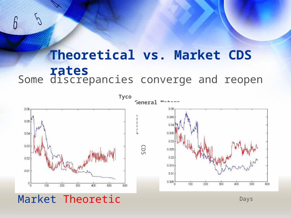
Theoretical vs. Market CDS rates

Some discrepancies converge and reopen Tyco General Motors

Market Theoretic

CD

S spread

Days

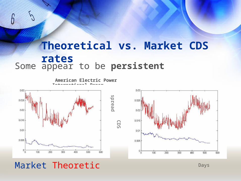
Theoretical vs. Market CDS rates

Some appear to be persistent American Electric Power International Paper

Market Theoretic

CD

S spread

Days

Caveats

• This is a convergence trading strategy• Spread may widen further, producing losses• Discrepancies may be from:

- Model or parameter misspecification

- Unperceived systematic risk factors

- Inherent liquidity differences

- “Genuine” mispricings

• NO guarantee that the difference will dissipate over a reasonable horizon

Strategy 1

• Many parameter combinations produce losses

• Many discrepancies do not converge

• We take on all openings & too many bad trades.

• Stop-loss is the dominating trade

• Maybe the biggest discrepancies are more likely to have genuine mispricings which converge?

Strategy 2: Rank and Hold

1. Rebalancing period length = T.

2. At each T, trade the top 10% discrepancies.

3. Take profits daily

4. At the end of T close everything, go back to 1.

→ We only trade egregious differences

→ We capture partial convergence during each holding period

Strategy 2 (cumulative P/L)

• H = 30

Flat regions meanno trades 10^4 $

• H = 60

Days

15 different combinations

gave positive P/L

Strategy 3: Active Holding Period

1. Interval length = I, Holding period = H

2. In strategy 2, we are idle during the holding periods but here we form new portfolios at every I.

3. At each I, close out the positions from t-H and form a new portfolio. Take profits daily.

Strategy 3 (cumulative P/L)

• (interval, hold) = (15,45) 10^4 $

Days

• (10,120)

Strategy 3 (cumulative P/L)

• (50,150)

10^4 $

• (40,160) Days

For combs tried cumP/L was positive Results seem more Volatile in the intervalLength than in H

Strategy 4: Capture the Momentum

In previous strategies we saw that wide differences may become wider.

Use a different ranking criteria: convergence momentum.

Similar to strategy 3, but compute and rank the rates of spread convergence during a lookback/formation period for each company

Strategy 4 (cumulative P/L)

• (15,30,60) interval = 15 10^4$

formation = 30

hold = 60

Days

• (15, 60,90)

Areas for Further Analysis 1. Margin effects.

2. Maximum draw-downs effect

3. Sharpe ratios analysis

4. Transaction costs

5. Out-of-sample testing

6. Leverage cycle strategies

7. Check constrained mean, long term time-averaged variance decay. Statistical arbitrage?

More of an instinct than science?

Appendix: Default Probabilities

• Monte Carlo is best, but too slow. Instead:

• We have formulas for option prices under q-alpha dynamics.

• The option surface implies the S distribution:

dP/dK = exp(-rT)Q{ST<K}

• Default probabilities computed by numerically differentiating deep OTM puts.