Embed Size (px)
Citation preview
1Journal of Insurance Issues, 2012, 35 (1): 1–43.Copyright © 2012 by the Western Risk and Insurance Association.All rights reserved.
Capital Structure in the Property‐Liability Insurance Industry:Tests of the Tradeoff and Pecking Order Theories
Jiang Cheng1 and Mary A. Weiss2
Abstract: This study examines whether property‐liability insurers have an optimumcapital structure by testing the tradeoff and pecking order theories for this industry.Capital structure is measured with the net premiums written to surplus ratio, andalternatively, with the liability to asset ratio. The results indicate that the tradeofftheory dominates the pecking order theory in explaining property‐liability insurercapital structure. Further, mutual and stock insurers appear to have different targetcapital structures, as agency theory suggests. Finally, mutual and stock insurers do notadjust at different speeds to their optimal capital structure. [Key words: Risk‐basedcapital, tradeoff theory, pecking order theory]
INTRODUCTION
tudies of firm capital structure are the subject of mainstream researchin the finance field (e.g., Shyam‐Sunder and Myers, 1999; Baker and
Wurgler, 2002; Fama and French, 2002; Welch, 2004; and Leary and Roberts,2005; Huang and Ritter, 2009; Leary and Roberts, 2010; Ovtchinnikov, 2010;among others). Two common theories to explain capital structure are thetradeoff theory and the pecking order theory.3 According to the tradeofftheory, firms “trade off” the benefits of holding capital (e.g., reduced
1Jiang Cheng, Ph.D. is assistant professor of Finance and Accounting at Shanghai Jiao TongUniversity, Shanghai, China. email: [email protected] A. Weiss, Ph.D. is Deaver Professor of Risk, Insurance & Healthcare Management atTemple University, Philadelphia, U.S.A., email: [email protected] appreciate valuable comments from David J. Cummins, Elyas Elyasiani, and seminarparticipants at the ARIA 2008 and the SRIA 2008 annual meetings. All errors are ours.
S
2 CHENG AND WEISS
chance of insolvency) with the costs of holding capital, including agencycosts, in arriving at an optimal or target capital level. Under the (modified)pecking order theory (Donaldson, 1961), firms finance their investmentswith the cheapest forms of capital, starting with internal capital and endingup with equity capital (as a last resort). Under this theory, a firm’s actualcapital structure depends on past profitability and prior investments.
In contrast to the finance literature on capital structure, there has beenrelatively little recent research on determinants of insurer capital structure.Some underwriting cycle theories focus on the relative “stickiness” ofcapital in the property‐liability insurance industry due to asymmetricinformation about such factors as the adequacy of loss reserves betweencapital providers and insurer managers (e.g., Winter, 1994; Cummins andDanzon, 1997; and Harrington and Niehaus, 2002). Other underwritingcycle theories posit that insurers have an optimal capital structure (e.g.,Cagle and Harrington, 1995; and Cummins and Danzon, 1997). Cumminsand Nini (2002) investigate whether insurers were overcapitalized in the1990s. But there has been no systematic test of mainstream finance theoriesabout capital structure such as the tradeoff and pecking order theories.
To better understand property‐liability insurer capital structure ingeneral, this research tests the tradeoff and pecking order theories in thisindustry. Tests of the tradeoff theory will indicate whether insurers havean optimal capital structure. On the other hand, the pecking order theoryposits no optimal capital structure. Instead, well‐financed insurers wouldhave an incentive to stockpile capital (as financial slack), and capitalizationwould not stabilize at some optimal levels as under the tradeoff theory.Thus, the pecking order and tradeoff theories can be tested by studying theresponse of well‐capitalized insurers to changes in relative capital levels.
Under the tradeoff theory, firms take actions to return to optimumcapital levels when deviations occur. However, adjusting capital structureis costly, and this may affect the speed at which firms return to optimumcapitalization. Therefore, in this research, a partial adjustment regressionmodel is estimated. This model allows us to determine whether an optimalcapital structure exists and thus whether the tradeoff or pecking ordertheory is supported. The partial adjustment model also allows us to esti‐mate the speed at which firms move toward their optimum or target, if anoptimum exists. Further, previous literature indicates that the speed with
3Other theories exist that are based on the market value of the firm (e.g., market timinghypothesis (Baker and Wurgler, 2002) and the inertia theory (Welch, 2004)). These theorieslikely have more limited applicability in the property‐liability insurance industry wheremany firms are not publicly traded (e.g., mutual insurers). Further, many publicly heldinsurers are part of a holding company, rather than traded individually.
RBC STRUCTURE 3
which firms return to their optimal capital structure varies by the degreeof undercapitalization, and tests for this are conducted in this research aswell (Lemmon and Zender, 2004; and Flannery and Rangan, 2006).
The sample period of this study is 1994 to 2003. Capital structure ismeasured using the net premiums written to surplus ratio, and, alternately,with the liability to asset ratio. Previous insurance literature employsleverage ratios such as these as a proxy for an insurer’s capitalization (e.g.,Cummins and Doherty, 2002; Cummins and Nini, 2002; and Harringtonand Niehaus, 2002); the finance literature also uses broad book leverageratios. Insurers are segmented into different categories based on their Risk‐based capital ratios to determine whether the financial strength of theinsurer affects adjustment speed. As a robustness measure, capital struc‐ture is measured also with the RBC ratio. The RBC ratio considers aninsurer’s surplus relative to the insurer’s risk, including underwriting risk.The advantage of this measure is that, unlike simple book measures ofleverage, it considers an insurer’s surplus level relative to the insurer’s risk,including underwriting, investment, and credit risk.4
This research is important for a number of reasons. This is the firststudy to directly test the tradeoff and pecking order theories in the prop‐erty‐liability insurance industry. Previously, these theories have beentested mainly in studies of non‐financial, unregulated industries. Also, thisresearch sheds light on the applicability of different underwriting cycletheories, such as the capacity constraint theory and other underwritingcycle theories that posit insurers have an optimal capital structure. That is,if insurers have an optimal capital structure, this would be consistent withthe tradeoff theory.
By way of preview, our results indicate that insurers do appear to havean optimal or target capital structure, and that some less well‐capitalizedinsurers move toward their target leverage ratios at different adjustmentspeeds. Well‐capitalized insurers with RBC ratios comfortably above theminimum requirement close about 20–30 percent of the gap between theirtarget and actual leverage ratio in one year. While the tradeoff theorydominates the pecking order theory, evidence exists that insurers’ capitalstructures are sensitive to financing deficits. The latter suggests that pastfinancing deficits affect the benefit‐cost tradeoff of holding capital. Finally,the results overall indicate that mutual and stock insurers have different
4Although the RBC ratio has been criticized in some previous studies as a measure ofrequired capital for an insurer (Cummins, Harrington, and Klein, 1995), it is the only ratioavailable that specifically incorporates the risk of an insurer. Further, an insurer may incurregulatory and other costs (such as loss of business) if it fails to meet RBC requirements,making the RBC ratio an important metric for insurers.

4 CHENG AND WEISS
target capital structures but differences in the speed of adjustment to theoptimal capital structure are mostly insignificant and not large in size.
The remainder of this paper is organized as follows. The next sectionbriefly summarizes the main capital structure theories tested, the tradeoffand pecking order theories, as they relate to the property‐liability insur‐ance industry specifically. The hypotheses are presented in the succeedingsection. The next section describes the capital structure measures used inthe study, the partial adjustment model, and factors expected to be associ‐ated with capital structure. This is followed by discussion of the data. Thesucceeding sections contain the results and the conclusion, respectively.
CAPITAL STRUCTURE THEORIES
The primary capital structure theories tested in this research are thetradeoff and pecking order theories. In this subsection, both of thesetheories are described. The discussion of these theories provides the back‐ground for the development of the hypotheses in the next section.
Tradeoff Theory
Under the tradeoff theory, market or regulatory forces are assumed todrive insurers to hold capital so as to maintain an acceptable insolvencyrisk. Then firms must balance the benefits against the costs of holdingcapital to achieve the optimal insolvency risk.5 Three main benefits areassociated with holding capital. First, insurance customers are sensitive tothe insolvency risk of an insurer, so an insurer may lose business if itsinsolvency risk becomes too high. Second, insurers with lower insolvencyrisk (“safer insurers”) can charge higher prices than insurers with higherinsolvency risk (Cummins and Danzon, 1997). Finally, insurers avoidfinancial distress costs by maintaining adequate capital levels. Financialdistress costs consist of costs such as direct and indirect bankruptcy costs,reputation losses, loss of valuable employees, and loss of investment inrelationship‐specific assets (e.g., investments in distribution systems orprivate information gained about customers).
But holding capital is costly. Insurers are subject to the costs of moralhazard and adverse selection in their claims settlement and underwritingactivities. Capital invested in an insurer is subject to double taxation, andother market imperfections can make holding capital costly (Cummins and
5Insurer capital is subject to fluctuation no matter how perfect contract design, underwrit‐ing, and the claims settlement processes of an insurer are, hence an insolvency risk isassumed to exist.

RBC STRUCTURE 5
Grace, 1994). Several different types of agency costs may affect capitalholding costs for insurers because of market frictions among policyholders,owners, and managers. The arguments concerning the balancing of bene‐fits and costs of holding capital have led some researchers to conclude thatinsurers have an optimal capital structure (e.g., Cagle and Harrington, 1995and Cummins and Danzon, 1997). The benefits and costs of holding capitalparticularly for property‐liability insurers are discussed below.
According to the general agency theory literature, managers areassumed to be risk‐averse, and as a result may be reluctant to take onpositive net present value (NPV) projects with high risk/variation that areexpected to increase firm value. Further, if managers do not have a fullownership stake, they may not exert their full effort because they do notreap the full rewards of their effort. And managers may behave in otherways that do not add value to the firm (e.g., excessive consumption ofperquisites, empire building). The possibility for opportunistic behaviorwould be enhanced for insurers that write long‐tail lines of insurance,because there is a longer time lag between receipt of cash premiums andpayout of losses. These agency costs may make capital more costly to holdfor these insurers.
Further, agency costs, and therefore capital structure, may also varyby organizational form. An inherent owner–policyholder conflict exists forinsurers whereby owners have an incentive to increase the risk of the firmto the detriment of policyholders. When policyholders are aware of thisconflict, the effect, in theory, is incorporated in price (i.e., a lower price mustbe charged). To mitigate the effect on price, owners can commit higherlevels of capital to the firm, and thus capital is less costly to hold as a result.The owner–policyholder conflict should not be a factor for mutual firms,because the owners and policyholders are the same.
Also, the manager–owner conflict may affect stock versus mutualinsurers differently because the owners of a mutual (the policyholders) donot exert much effective control over managers (Mayers and Smith, 1992and 2005; and Mayers, Shivdasani, and Smith, 1997). This would makecapital more costly to hold for mutual insurers, everything else held equal.
On the other hand, mutuals have less access to capital markets, makingraising capital more difficult and costly for them (e.g., Harrington andNiehaus, 2002). Hence for a mutual, holding capital may be less costly thanthe alternative of raising capital when capital is needed. Mutuals mightfind it less costly to hold capital than stocks, according to this argument.
In summary, inherent differences in the owner–policyholder conflictand owner–manager conflict in mutual versus stock insurers and the factthat mutuals may find it more difficult to raise capital may result indifferent optimal capital structures for stock versus mutual insurers. On

6 CHENG AND WEISS
the other hand, mutual and stock insurers should experience similar capitalholding costs with respect to adverse selection and moral hazard, doubletaxation and costs associated with other market imperfections.6
According to the tradeoff theory, not only is holding capital costly butso is adjusting capital structure.7 One primary reason capital adjustment iscostly is the existence of information asymmetries between managers andinvestors (Myers and Majluf, 1984). In the property‐liability insuranceindustry, this problem is particularly applicable due to informationalasymmetries about the adequacy of loss reserve levels. Loss reserves arethe single largest liability for property‐liability insurers, accounting for 56percent of total industry liabilities in 2005 (Best’s Aggregates & AveragesProperty/Casualty, 2006). Managers are much more knowledgeable aboutloss reserve levels and might manipulate loss reserves (Weiss, 1985; Petroni,1992; and Gaver and Paterson, 2004). Thus the adequacy of prices, lossreserves, and the risk of the firm are more difficult for investors to deter‐mine in this industry compared to some others. As a result, raising equitycapital for insurers is likely to be more costly compared to firms in mostother industries, and an insurer may not always be at its optimal capitallevel if increasing capital is costly in the short term.
Pecking Order Theory
The pecking order theory also is based on informational asymmetriesbetween equity providers and firm managers. According to this theory,informational asymmetries between firms and investors imply that exter‐nal capital is likely to be more costly than internal capital (Myers, 1984;Froot, Scharfstein, and Stein, 1993). Therefore, firms prefer to use internalcapital first in financing investments. If external financing is required,firms’ next choice will be safe debt. Equity issuance is a last resort forinvestment financing because it is the most costly (Myers and Majluf, 1984).An optimal capital level does not exist under this theory, as firms prefer toaccumulate financial slack for future investment purposes. According tothis theory, current capital levels will be directly related to the net changesin the firm’s external and internal cash flows (i.e., the financing deficit).8Support for this theory can be found in underwriting cycle theory. Under
6Some arguments explaining the mutual form of organization stress the shared nature oflosses associated with the mutual form of organization (e.g., Thistle and Ligon, 2005). Underthese theories, mutuals may be less subject to adverse selection and moral hazard as a result.7The static tradeoff theory of capital structure assumes that the cost of adjusting an insurer’scapital structure is zero. In dynamic versions of the model, the optimum is characterized asan optimal interval, and active revisions in the firm’s capital structure occur when the end‐points of the interval are violated (Fisher, Heinkel, and Zechner, 1989).
RBC STRUCTURE 7
the capacity constraint theory, capital does not flow freely into and outof the property‐liability insurance industry (Winter, 1994). Insurers antici‐pate that correlation among losses will lead to loss shocks that depletecapital. Thus in periods of excess capacity (when the industry is flush withcapital), insurers will hold on to capital. Also, because internal capital ischeaper than external capital, firms prefer to raise capital through retainedearnings.
Because the property‐liability insurance industry consists of mutualversus stock insurers, and stock insurers have easier access to equitymarkets, the implication of the pecking order theory may be different forstock and mutual insurers. More specifically, stock insurers may be lessreliant on financial slack than are mutuals.
Hypotheses
The pecking order theory predicts that a typical insurer does not havea target capital ratio, while the tradeoff theory indicates that an optimaltarget capital level based on a benefit‐cost tradeoff exists. Thus the firsthypothesis is concerned with whether the tradeoff theory is supported:
Hypothesis 1: The tradeoff theory dominates the pecking order theory inexplaining insurer behavior over the sample period.
The sample period of 1994 to 2003 is especially interesting to study,since the imposition of new RBC requirements in 1994 may have changedthe regulatory costs associated with holding capital (and thus, the optimalcapital level).
Lemmon and Zender (2004) argue that undercapitalized firms have nochoice but to improve capitalization, because they cannot borrow furtherin the market. With respect to property‐liability insurers, undercapitalizedinsurers would have an incentive to improve their capital position regard‐less of whether the pecking order theory or tradeoff theory is more impor‐tant. Thus, the pecking order theory and tradeoff theory have the sameprediction for undercapitalized insurers. Therefore, Hypothesis 1 is testedfor well‐capitalized property‐liability insurers. Intuitively, Hypothesis 1 istested with a regression model that determines the extent to which changesin capital at t+1 are related to capital at time t and the financing deficit.9The pecking order theory would be supported if the economic significance
8The financing deficit is defined by Frank and Goyal (2003) as external cash outflow (i.e., thesum of dividend payments, investments, and change in working capital) net of internal cashflow divided by total assets. 9Of course, other firm characteristics are controlled for in the regression model.
8 CHENG AND WEISS
of the financing deficit variable outweighed the importance of capital inthe model.
The discussion in the previous section indicates that the higher cost ofraising capital should lead mutuals to hold more capital, while agency costsassociated with the owner–policyholder conflict and manager–owner con‐flict should reduce the costs of holding capital for stock insurers. Therefore,under the tradeoff theory, if the benefits and costs of holding capital varyby organizational form, then the target capital level would be different forstocks and mutuals. Thus Hypothesis 1a states,
Hypothesis 1a: Mutual and stock insurers do not have the same target capitallevel.
Harrington and Niehaus (2002) find evidence that capital‐to‐liability ratiosare relatively higher for mutuals than for stock insurers.
Further, since mutuals have less access to capital markets, mutualswould be expected to adjust more slowly to their target capital level,leading to Hypothesis 1b,
Hypothesis 1b: Mutual insurers adjust more slowly to their target capitallevel than stock insurers.
This hypothesis was supported by Harrington and Niehaus (2002).Agency costs associated with the manager–owner conflict should
affect the cost of holding capital for firms writing predominantly long‐taillines, per the discussion in the previous section. This leads to Hypothesis1c:
Hypothesis 1c: Insurers writing relatively more long‐tail lines have lowertarget capital levels.
Under the pecking order theory, the financing deficit is the most importantdeterminant of a firm’s capital structure. However, it is possible that thefinancing deficit is a consideration in determining optimal capital structureunder the tradeoff theory.10 That is, the relative costs of using internal cashflows for funding versus external sources may be one of the factors thatinsurers “trade off” in determining capital structure (Frank and Goyal,2003, p. 219). For example, more‐profitable insurers in the industry mightrely more on internal capital to finance investments because it is cheaper(pecking order theory), while still maintaining a target capital level
10Froot (2007) argues that insurers can invest more aggressively with a high level of capitalalthough the deadweight costs of holding capital must be considered. He also indicates thatthe insurer might hold more capital if there were product‐market imperfections besides cap‐ital‐market imperfections.
RBC STRUCTURE 9
(tradeoff theory). The discussion in the preceding section indicates thatmutual firms should find it relatively more difficult to raise capital whenfinancing deficits (e.g., underwriting losses) occur, leading to Hypothesis1d:
Hypothesis 1d: Mutual firms’ capital levels are more sensitive to financingdeficits than stock insurers.
In their study of unregulated, non‐financial firms, Flannery and Ran‐gan (2006) found evidence that firms with relatively low capital levels movetoward their targets more quickly than those with a high capital level. Thissuggests that deviations from target levels are more costly for under‐capitalized firms. If this were also true in the property‐liability insuranceindustry, then less well‐capitalized insurers would be expected to improvetheir capital position at a greater speed than well‐capitalized insurers. Thusthe second hypothesis states,
Hypothesis 2: Insurers in varying financial condition adjust toward theirtarget capital level at different speeds, with less well‐capitalized insurersadjusting more quickly to their target capital level than well‐capitalizedinsurers.
METHODOLOGY
In this section, the selection of the capital structure variables andcategorization of insurers into well‐capitalized versus less well‐capitalizedare discussed, followed by a description of the partial adjustment modelused to test the pecking order and tradeoff theories. Finally, factorsexpected to be associated with capital structure that are used in the partialadjustment model are explained.
Capital Level Measure
Ideally the measure of capitalization used to test the capital structuretheories should reflect important characteristics and the risk of the insurer.The best readily available candidates for measuring capital levels are thenet premiums written to surplus ratio and the liability to assets ratio(Cummins and Doherty, 2002; Cummins and Nini, 2002; and Harringtonand Niehaus, 2002).
To test hypotheses regarding adjustment speed for firms in varyingfinancial condition, insurers must be classified as well‐capitalized versusless well‐capitalized. This is achieved by means of the RBC ratio. The RBCratio is defined as the ratio of an insurer’s total adjusted capital to risk‐based capital. More specifically, an insurer is categorized into one of five
10 CHENG AND WEISS
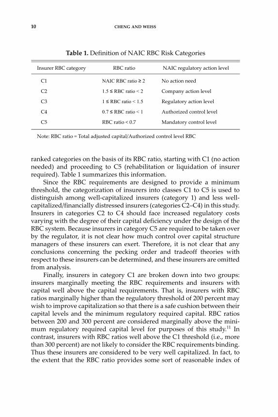
ranked categories on the basis of its RBC ratio, starting with C1 (no actionneeded) and proceeding to C5 (rehabilitation or liquidation of insurerrequired). Table 1 summarizes this information.
Since the RBC requirements are designed to provide a minimumthreshold, the categorization of insurers into classes C1 to C5 is used todistinguish among well‐capitalized insurers (category 1) and less well‐capitalized/financially distressed insurers (categories C2–C4) in this study.Insurers in categories C2 to C4 should face increased regulatory costsvarying with the degree of their capital deficiency under the design of theRBC system. Because insurers in category C5 are required to be taken overby the regulator, it is not clear how much control over capital structuremanagers of these insurers can exert. Therefore, it is not clear that anyconclusions concerning the pecking order and tradeoff theories withrespect to these insurers can be determined, and these insurers are omittedfrom analysis.
Finally, insurers in category C1 are broken down into two groups:insurers marginally meeting the RBC requirements and insurers withcapital well above the capital requirements. That is, insurers with RBCratios marginally higher than the regulatory threshold of 200 percent maywish to improve capitalization so that there is a safe cushion between theircapital levels and the minimum regulatory required capital. RBC ratiosbetween 200 and 300 percent are considered marginally above the mini‐mum regulatory required capital level for purposes of this study.11 Incontrast, insurers with RBC ratios well above the C1 threshold (i.e., morethan 300 percent) are not likely to consider the RBC requirements binding.Thus these insurers are considered to be very well capitalized. In fact, tothe extent that the RBC ratio provides some sort of reasonable index of
Table 1. Definition of NAIC RBC Risk Categories
Insurer RBC category RBC ratio NAIC regulatory action level
C1 NAIC RBC ratio ≥ 2 No action need
C2 1.5 ≤ RBC ratio < 2 Company action level
C3 1 ≤ RBC ratio < 1.5 Regulatory action level
C4 0.7 ≤ RBC ratio < 1 Authorized control level
C5 RBC ratio < 0.7 Mandatory control level
Note: RBC ratio = Total adjusted capital/Authorized control level RBC
RBC STRUCTURE 11
adequate capitalization, insurers with the highest RBC ratios could facepressure to reduce their ratios.12
Partial Adjustment Model Specification and Estimation
A partial adjustment model is used to determine whether firms behaveas if they have a target capital structure and the speed at which firms adjustto their target capital structure (assuming they have a target capital struc‐ture). The partial adjustment model allows for the existence of adjustmentcosts that may prevent an insurer from returning immediately to the targetcapital structure. Instead, return to the target capital structure may requireseveral periods.
The optimal capital structure is not directly observable, and it is likelyto differ across individual insurers and/or over time. To allow for this, thefollowing general target capital structure equation is estimated:
(Capital ratio)*i,t+1 = βXit, (1)
where (Capital ratio)*i,t+1 is the measure of target capital structure (i.e.,leverage ratio) for insurer i in year t+1, Xit is a vector of insurer character‐istics related to costs and benefits of operating at that capital structure, andβ represents a vector of coefficients.13 A standard partial adjustment modelis given by
(Capital ratio)i,t+1 – (Capital ratio)i,t =
δ[(Capital ratio)*i,t+1 – (Capital ratio)i,t] + εi,t+1. (2)
11Initially, insurers in the bottom 10 percent of the C1 sample were considered to be margin‐ally above the threshold; however, the RBC ratio at this observation (3.46909) was shared bymany other insurers both above and below the 10 percent cutoff level (i.e., a total of 788insurers had this RBC ratio). The next smallest RBC ratio after 3.46909 was 2.96125. There‐fore, this RBC ratio (rounded to three) was used to find insurers marginally above thethreshold. As a robustness test, the sample of insurers with RBC ratios lower than 3.46909(or 11.5 percent of the C1 sample) were considered to be marginally above the threshold,and analysis was conducted with this sample. However, the results were not significantlychanged when this subsample was used. 12Although the RBC ratio has been criticized in some previous studies as a measure ofrequired capital for an insurer (Cummins, Harrington, and Klein, 1995), it is the only ratioavailable that specifically incorporates the risk of an insurer. Further, an insurer may incurregulatory and other costs (such as loss of business) if it fails to meet RBC requirements,making the RBC ratio an important metric for insurers. 13There is no stochastic disturbance term εit in equation (1). If (Capital ratio)*i,t+1 is truly anequilibrium relation, an error term is not required. On the other hand, the adjustment mech‐anism can be imperfect, in which case an error term should be added.
12 CHENG AND WEISS
Equation (2) indicates that the actual change in the capital ratio in anygiven time period t+1 is some fraction δ of the desired change for thatperiod. If δ = 1, then the insurer adjusts to the desired capital ratioinstantaneously in the same period. However, if δ = 0, then the actualcapital ratio at time t+1 is the same as that observed in the previous timeperiod t so that nothing has changed. Typically, δ is expected to lie betweenthese two extremes since the individual insurer is likely to close a propor‐tion δ of the gap between its actual and its desired capital ratio, if thetradeoff theory applies.
After substituting equation (1) into equation (2) and doing somerearranging, the model becomes:
(Capital ratio)i,t+1 = (δβ)Xit + (1–δ) (Capital ratio)i,t + εi,t+1. (3)
Equation (3) implies that (1) insurers have target capital ratios, which areequal to βXit (from equation (1)); (2) insurers take steps to close the gapbetween the target and existing capital ratio within each time period; and(3) the short‐run adjustment speed δ is the same for all insurers and givenby 1 minus the estimated coefficient of (Capital ratio)i,t.14 Hypothesis 1would be partly supported if the coefficient for (Capital ratio)i,t is signifi‐cant and less than one.15
Testing Speed of Adjustment. To test some hypotheses, a distinctionbetween mutual and stock insurers is required or a distinction betweeninsurers in different financial condition (i.e., different RBC categories) mustbe made. The discussion illustrating how these hypotheses will be testedis framed in terms of the hypotheses concerning stock versus mutualinsurers. However, the methodology used to distinguish between insurersin varying financial condition is analogous to that used for distinguishingstock versus mutual insurers.
The partial adjustment models for stock and mutual insurers areassumed to be:
(Capital ratio)Si,t+1 = (δSβS)XSit + (1 – δS) (Capital ratio)Sit + εSi,t+1 (4a)
14The equation also implies that the long‐run impact of firm characteristics on the leverageratio is given by the estimated coefficients of Xit divided by δ.15The way the problem of mechanical mean reversion in the leverage ratio is dealt with issimilar to Flannery and Rangan (2006). That is, the sample is sorted into several categoriesby RBC ratio as well as by organizational form. This approach at least partly deals with anymechanical mean reversion problem that may exist (Chen and Zhao, 2007).
RBC STRUCTURE 13
(Capital ratio)Mi,t+1 = (δMβM)XMit + (1 – δM) (Capital ratio)Mit + εMi,t+1, (4b)
where S and M represent stock and mutual insurers, respectively. To allowfor the possibility that mutual and stock insurers have different adjustmentspeeds as well as different capital structure, the following pooled modelcan be estimated:
(Capital ratio)Ai,t+1 = DS[ (δSβS)XSit + (1 – δS) (Capital ratio)Sit] +
DM [ (δMβM)XMit + (1 – δM) (Capital ratio)Mit] + εAi,t+1, (5)
where A represents a stock or mutual insurer and DM (DS) is a dummyvariable equal to one if the insurer is a mutual (stock) insurer.
If βS ≠ βM, this would indicate that mutuals’ target capital ratios aredifferent from stock insurers, supporting Hypothesis 1a. Further, the indi‐vidual coefficients for each Xi can be compared across stock and mutualinsurers to determine what causes any difference in capital structure,assuming a difference is found. Finally, if δS is significantly different fromδM , then this would signify that mutuals adjust toward their capitalstructure at a different speed than stock insurers. In particular, if δS > δM,then mutuals adjust more slowly toward their optimal capital structurethan stock insurers, supporting Hypothesis 1b.
To test Hypothesis 2, Equation (5) is modified as follows:
(Capital ratio)Bi,t+1 = DCn[ (δCnβCn)XCnit + (1 – δCn) (Capital ratio)Cnit] +
DCp [ (δCpβCp)XCpit + (1 – δCp) (Capital ratio)Cpit] + εBi,t+1, (6)
where Cn and Cp refer to insurers with specific RBC ratio ranges definedin terms of categories n and p, respectively. The subscript B applies toinsurers in categories Cn and Cp (i.e., a pooled sample of insurers incategories Cn and Cp). Also, Cp refers to a category of insurers with RBCratios less than that for insurers in Cn (i.e., insurers in Cp have lower relativecapitalization). Note that equation (6), like equation (5), allows all coeffi‐cients for the Cn variables to vary from those for Cp.
If insurers in varying financial condition adjust toward their targetcapital level at different speeds, then the coefficient for (Capital Ratio)Cnitwould be significantly different from for (Capital Ratio)Cpit, and Hypothe‐sis 2 is supported. In particular, if insurers that are less well‐capitalizedadjust toward their target capital structure more quickly, then δCp > δCn, andHypothesis 2 would be supported. Equation (6) is estimated for the follow‐ing samples of insurers: (a) insurers with RBC ratio > 3 versus insurers with2 ≤ RBC ratio ≤ 3; (b) insurers with 2 ≤ RBC ratio ≤ 3 versus insurers in RBC
14 CHENG AND WEISS
category C2; and (c) insurers in category C2 versus insurers in categoriesC3–C4.
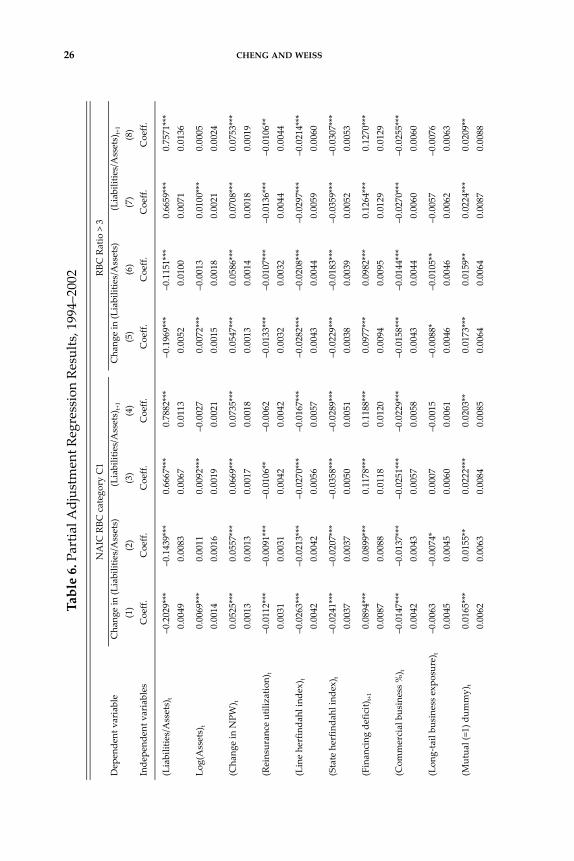
Testing Dominance of Tradeoff Theory. As indicated previously,under the pecking order theory, the financing deficit is the primary factorin explaining contemporaneous changes in a firm’s capital structure. Thusto test this theory, the relationship between changes in an insurer’s capitalstructure (i.e., leverage ratio) and the financing deficit must be determinedin relation to other factors associated with the tradeoff theory:
∆(Capital ratio)i,t+1 = (δβ)Xit – δ(Capital ratio)i,t +
λ(Financing deficit)i,t+1 + εi,t+1, (7)
where ∆(Capital ratio)i,t+1 = (Capital ratio)i,t+1 – (Capital ratio)i,t and the othervariables are defined as before (Flannery and Rangan, 2006). The coefficientλ is expected to be positive and significant under the pecking order theory,if a leverage ratio is used as the dependent variable. Furthermore, theeconomic impact of this variable should far outweigh the effect of thelagged capital ratio on ∆(Capital ratio)i,t+1. That is, the effect of the otherexplanatory variables in the equation should decrease significantly inimportance so that the change in the capital ratio (or leverage ratio) isexplained primarily by the financing deficit (Frank and Goyal, 2002). If thelatter occurs, then the pecking order theory would dominate the tradeofftheory. Otherwise, Hypothesis 1 would be supported. For reasonsexplained earlier, equation (7) is estimated for relatively well capitalizedinsurers (i.e., insurers in category C1).
To determine whether the tradeoff or pecking order theory is relativelymore important for stock versus mutual insurers, the change in the capitalratio from equation (5) is estimated:
∆(Capital ratio)Ai,t+1 = [(Capital ratio)Ai,t+1 – (Capital ratio)Ait] =
DS[(δSβS)XSit – δS(Capital ratio)Sit + λS(Financing deficit)Si,t+1] +
DM[(δMβM)XMit – δM(Capital ratio)Mit +
λM(Financing deficit)Mi,t+1] + εAi,t+1. (8)
A positive coefficient for the financing deficit variable would meanthat an insurer’s level of capitalization (leverage) increases directly withfinancing deficits.16 Thus, if the coefficients λS and λM are positive and
16Recall that the financing deficit is scaled net cash outflow. Thus, if the financing deficit isgreater than zero, then the firm’s cash position has deteriorated.

RBC STRUCTURE 15
significant and also outweigh the importance of the other variables in thechange in leverage ratio equations, the pecking order theory would besupported. If ??? the absolute value of ? λM exceeds that of λS, this wouldindicate that changes in mutual insurers’ leverage ratios are more sensitiveto mutuals’ financing deficits, supporting Hypothesis 1d. Finally, if thecoefficient λS(λM) only is significant, and its economic impact outweighsthe other regression variables, this would signify that the pecking ordertheory is dominant for stock (mutual) insurers only, contradicting (sup‐porting) Hypothesis 1d.
Estimation Techniques
We first estimate pooled regression models based on equations (3), (5),(6), (7), and (8) using OLS, a firm fixed effects model, and a firm randomeffects model for all regressions.17 Time dummy variables are included inthe regressions to control for any time‐varying influences on capital struc‐ture (e.g., regulatory environment change, catastrophe risk shocks, andmacroeconomic environment changes). Finally, because inclusion of alagged dependent variable can result in correlation between this variableand the error term, models using two‐stage‐least‐squares are estimated aswell.18 Consistent with prior research, the data are winsorized (at the 5thand 95th percentile), to eliminate extreme observations (see, e.g., Flanneryand Rangan, 2006). Nonlinear wald tests are performed to determinewhether the individual coefficients comprising βS are different from βM.19
Determinants of Target Capital Structure
Before equation (3) can be estimated, the determinants of capitalstructure (Xit), must be specified. The hypotheses provide some guidanceon the variables that should be included in Xit. Hypothesis 1c indicates thatinsurers writing relatively more long‐tail lines of business should havelower target capital levels. Therefore, a long‐tail lines variable defined as(total loss reserves)/(total losses incurred) is included in the regression
17The partial adjustment model satisfies the assumptions of the classical linear regressionmodel, and OLS estimation will yield consistent estimates (Gujarati, 2003: 677). Flanneryand Rangan (2006) suggest that a panel regression with unobserved (fixed) effects is moreappropriate if firms have relatively stable, unobserved variables affecting their leverage tar‐gets.18 STATA’s software for two‐stage‐least squares is used in the estimation, and the standarderror of the coefficient for the endogenous regression variable is adjusted as part of the two‐stage least squares routine. See Davidson and MacKinnon (1993: 209–224).19 That is, the coefficients estimated are δSβS and δMβM. Thus a wald test is conducted todetermine whether δSβS/δS = δMβM/δM.
16 CHENG AND WEISS
(Cummins and Nini, 2002). Hypothesis 1c is supported if the coefficient forthis variable is negative.
Prior literature indicates that additional factors are associated withinsurer capital structure. Insurers that are more diversified are expected torequire less relative capital to operate. Size is sometimes associated withdiversification because larger insurers, in theory, should be able to achievea better spread of risk than smaller insurers. Therefore size, defined as thelogarithm of assets, is included in the regression model, and its expectedsign is positive. Insurers might also diversify risk by writing across manydifferent product lines and/or across different geographic areas. Therefore,herfindahl indices for product mix and geographic spread are included inthe model. The expected signs for the herfindahl index variables arenegative. That is, decreases in product mix and geographic spreads areassociated with increases in the herfindahl index and less diversification.Less diversification would be associated with higher capital requirements(i.e., lower leverage). Reinsurance usage is associated with increased diver‐sification, since through reinsurance insurers can obtain a better spread ofrisks (Cummins and Nini, 2002). Reinsurance usage is measured as theratio of ceded loss reserves to the sum of direct loss reserves and assumedloss reserves. Reinsurance usage is expected to be positively related toleverage.
Growth opportunities are expected to be related to capital structure.Firms with growth opportunities should prefer to finance these with thecheapest form of capital, internal capital. Further, asymmetries betweenmanagers and investors are also likely to make financing new investmentsthrough internal capital to be preferred (Myers and Majluf, 1984). Thus,firms with more growth opportunities are expected to hold relatively morecapital, everything else equal. Growth opportunities are measured as thechange in direct net premiums written. However, insurers experience anequity penalty when writing new business. That is, prepaid acquisitionexpenses (an asset under GAAP accounting) are not recognized as an assetin statutory accounting. Instead, prepaid acquisition expenses effectivelyact to reduce underwriting income and, hence, surplus or equity. Therefore,the sign of the growth variable is difficult to predict.
As mentioned earlier, the financing deficit can be a factor consideredunder the tradeoff theory. That is, it is possible that a significant andpositive coefficient might be found for the leverage ratios, but that the netexternal and internal cash flows still play a role in determining capitalstructure. (That is, the financing deficit could be just one of several factorsconsidered by a firm in setting target capital structure.) Therefore, thefinancing deficit variable is included when estimating equation (5), and itsexpected sign is positive for the reasons discussed earlier.20 Commercial

RBC STRUCTURE 17
business is sometimes considered to be more volatile than personal linesof business (such as personal auto); thus the percent of business written incommercial lines is included in the model. The expected sign for thisvariable is negative.
A dummy variable representing group affiliation is included in themodels. Group insurers might have an advantage by being able todiversify risks within the group (through intra‐group reinsurance) andoperate with relatively lower capital levels. On the other hand, insurerswithin a group might be more likely to obtain capital infusions from theirparent company when capital levels are deficient. Therefore, the sign forthis variable is difficult to predict a priori. Finally, a dummy variableequal to one for insurers that are neither mutuals nor stocks (and zerootherwise) is included in the model. We have no priors on the sign ofthis variable.
DATA
Individual insurer data are used in this study because RBC standardsapply to individual insurers and state regulators focus more on individualinsurers’ insolvency propensities than that of groups (Cummins, Har‐rington, and Klein, 1995). Data were obtained primarily from individualinsurers’ Annual Statements filed with the NAIC. The sample insurersconsist of insurers included in the NAIC’s RBC database; this databaseexcludes certain specialty insurers and insurers that did not file a statementwith the NAIC.21 All insurers with negative assets, surplus, and net premi‐ums written are excluded.22 Further, data for two consecutive years were
20Prior studies have also considered whether firms’ capital adequacy is related to past prof‐itability and to cash flow (e.g., Harrington and Niehaus, 2002; Rajan and Zingales, 1995; andBaker and Wurgler, 2001). 21Insurers excluded from the NAIC filing requirements are typically reinsurers, small sin‐gle‐state companies, or small companies with exotic organizational forms such as TexasLloyds or reciprocals (Cummins, Grace, and Phillips, 1999). Professional reinsurers areexcluded. Following Weiss and Chung (2004), an insurer is classified as a professional rein‐surer if the proportion of its property‐liability nonproportional reinsurance premiumsassumed from nonaffiliates exceeds 70 percent of its total reinsurance assumed. This isbased on the criterion that professional reinsurers will not rely extensively on intra‐grouptransactions. Any insurers classified by the NAIC as “U.S. branch of alien insurer” areexcluded from the sample. 22Insolvent insurers are not included in the study since these insurers are already under thecontrol of the regulator through the liquidation or rehabilitation process and consequentlydo not make independent business decisions. Their data also are typically unavailable in theNAIC Annual Statement database.
18 CHENG AND WEISS
required for each sample insurer; hence observations that did not meet thiscriterion were eliminated from the sample.23 The final sample has 17,393firm‐year observations.24
RESULTS
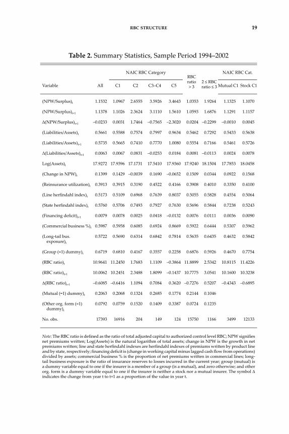
Summary statistics for the samples analyzed in this research arepresented in Table 2. Means for the entire sample and by NAIC categori‐zation are provided as well as means for stock and mutual insurers incategory C1. Insurers in categories C3 and C4 are combined into onesample because there were too few observations to analyze categories C3and C4 separately.
As expected, insurers in category C1 have much lower leverage ratiosthan insurers in the other NAIC categories. Asset size (expressed in loga‐rithms), percent of business in commercial lines, and the long‐tail linesvariables do not appear to vary substantially among the different samples,however (except for category C5). Mutuals have significantly lower ratiosof liabilities to assets than stocks do and this is consistent with Harringtonand Niehaus (2002).25 Change in net premiums written varies substantiallyamong the samples, and it is highest for insurers in categories C1 and C3–C4. The herfindahl indices for lines of business and state geographic spreadalso vary among the categories, with higher indices observed for insurersin the lower‐rated NAIC categories. Membership in an insurance group islower for insurers in lower‐rated RBC categories.
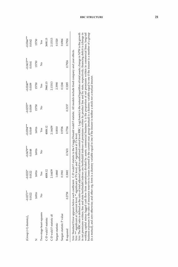
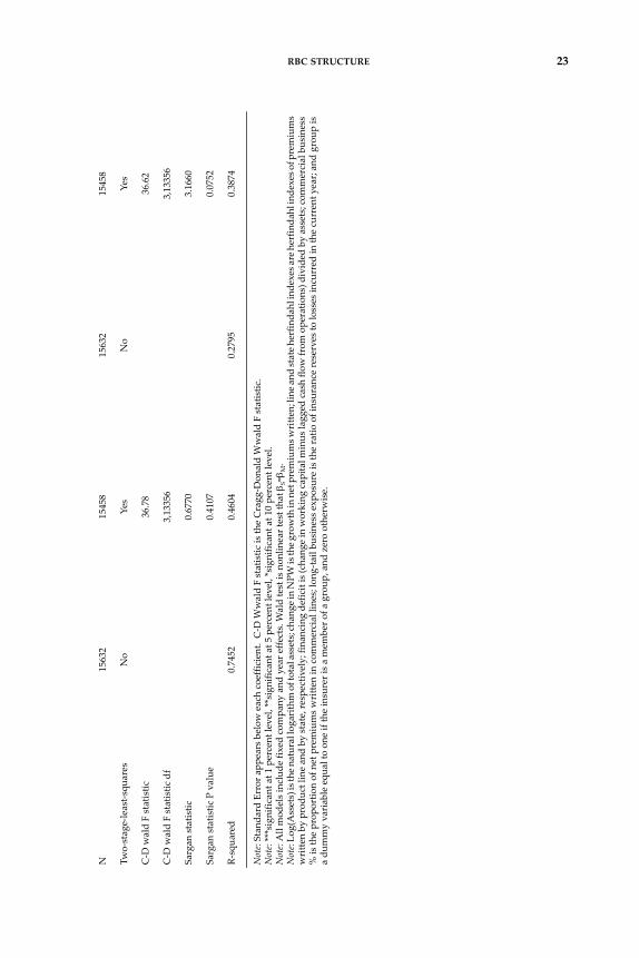
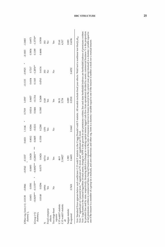
In the remainder of this section, tests of the specific hypotheses arediscussed. The hypotheses tests are based on the results of partial adjust‐ment model regressions on various (sub)samples of the data. The regres‐sion results are presented in Tables 3 through 8, with Tables 3 through 5providing results for regressions in which NPW/Surplus is used as theleverage ratio and Tables 6 through 8 providing results for regressions inwhich Liabilities/Assets is used as the dependent variable.
Panel data methods are used in estimation for all cases where adequatenumbers of observations for the same insurer over time are included in the
23For example, the leverage ratios for two consecutive years are used in equation (3), and tocompute the change in net premiums written, two consecutive years of data are needed.24The numbers of observations in the final sample for 1994 through 2003, by year, are 1590,1799, 1800, 1798, 1798, 1723, 1698, 1730, 1727, and 1730, respectively.25Harrington and Niehaus (2002) argue that mutuals have higher ex ante target capital ratiosthan stock insurers. Mutuals also have a higher ratio of NPW to Surplus, but the differenceis not significant at conventional significance levels. The latter is not consistent with Har‐rington and Niehaus (2002).
RBC STRUCTURE 19
Table 2. Summary Statistics, Sample Period 1994–2002
Variable
NAIC RBC CategoryRBC ratio> 3
2 ≤ RBCratio ≤ 3
NAIC RBC Cat.
All C1 C2 C3–C4 C5 Mutual C1 Stock C1
(NPW/Surplus)t 1.1532 1.0967 2.6555 3.5926 3.4643 1.0353 1.9264 1.1325 1.1070
(NPW/Surplus)t+1 1.1378 1.1026 2.3624 3.1110 1.5610 1.0593 1.6876 1.1291 1.1157
∆(NPW/Surplus)t+1 –0.0233 0.0031 1.7464 –0.7565 –2.3020 0.0204 –0.2299 –0.0010 0.0045
(Liabilities/Assets)t 0.5661 0.5588 0.7574 0.7997 0.9634 0.5462 0.7292 0.5433 0.5638
(Liabilities/Assets)t+1 0.5735 0.5665 0.7410 0.7770 1.0080 0.5554 0.7166 0.5461 0.5726
∆(Liabilities/Assets)t+1 0.0063 0.0067 0.0831 –0.0253 0.0184 0.0081 –0.0113 0.0024 0.0078
Log(Assets)t 17.9272 17.9396 17.1731 17.5410 17.9360 17.9240 18.1504 17.7853 18.0458
(Change in NPW)t 0.1399 0.1429 –0.0039 0.1690 –0.0652 0.1509 0.0344 0.0922 0.1568
(Reinsurance utilization)t 0.3913 0.3915 0.3190 0.4522 0.4166 0.3908 0.4010 0.3350 0.4100
(Line herfindahl index)t 0.5173 0.5109 0.6968 0.7639 0.8037 0.5055 0.5828 0.4554 0.5064
(State herfindahl index)t 0.5760 0.5706 0.7493 0.7927 0.7630 0.5696 0.5844 0.7238 0.5243
(Financing deficit)t+1 0.0079 0.0078 0.0025 0.0418 –0.0132 0.0076 0.0111 0.0036 0.0090
(Commercial business %)t 0.5987 0.5958 0.6085 0.6924 0.8669 0.5922 0.6444 0.5307 0.5962
(Long‐tail bus. exposure)t
0.5722 0.5690 0.6314 0.6842 0.7814 0.5635 0.6435 0.4632 0.5842
(Group (=1) dummy)t 0.6719 0.6810 0.4167 0.3557 0.2258 0.6876 0.5926 0.4670 0.7754
(RBC ratio)t 10.9641 11.2450 1.7683 1.1109 –0.3864 11.8899 2.5342 10.8115 11.4226
(RBC ratio)t+1 10.0062 10.2451 2.3488 1.8099 –0.1437 10.7775 3.0541 10.1600 10.3238
∆(RBC ratio)t+1 –0.6085 –0.6416 1.1094 0.7084 0.3620 –0.7276 0.5207 –0.4343 –0.6895
(Mutual (=1) dummy)t 0.2063 0.2068 0.1324 0.2685 0.1774 0.2144 0.1046
(Other org. form (=1) dummy)t
0.0792 0.0759 0.1520 0.1409 0.3387 0.0724 0.1235
No. obs. 17393 16916 204 149 124 15750 1166 3499 12133
Note: The RBC ratio is defined as the ratio of total adjusted capital to authorized control level RBC; NPW signifiesnet premiums written; Log(Assets) is the natural logarithm of total assets; change in NPW is the growth in netpremiums written; line and state herfindahl indexes are herfindahl indexes of premiums written by product lineand by state, respectively; financing deficit is (change in working capital minus lagged cash flow from operations)divided by assets; commercial business % is the proportion of net premiums written in commercial lines; long‐tail business exposure is the ratio of insurance reserves to losses incurred in the current year; group (mutual) isa dummy variable equal to one if the insurer is a member of a group (is a mutual), and zero otherwise; and otherorg. form is a dummy variable equal to one if the insurer is neither a stock nor a mutual insurer. The symbol Δindicates the change from year t to t+1 as a proportion of the value in year t.

20 CHENG AND WEISSTable 3. Partia
l Adjustm
ent R
egression Re
sults, 1994–2002
NAIC RBC category C1
RBC ra
tio > 3
Dep
ende
nt variable
Cha
nge in N
PW/Surplus
(NPW
/Surplus) t+
1Cha
nge in N
PW/Surplus
(NPW
/Surplus) t+
1
Inde
pend
ent v
ariables
(1)
Coeff.
(2)
Coeff.
(3)
Coeff.
(4)
Coeff.
(5)
Coeff.
(6)
Coeff.
(7)
Coeff.
(8)
Coeff.
(NPW
/Surplus) t
–0.2549***
–0.2170***
0.6504***
0.7168***
–0.1883***
–0.1728***
0.7010***
0.7525***
0.0055
0.0092
0.0067
0.0112
0.0055
0.0091
0.0072
0.0117
Log(Assets)
t0.0737***
0.0660***
0.0797***
0.0662***
0.0525***
0.0492***
0.0687***
0.0580***
0.0072
0.0073
0.0087
0.0090
0.0066
0.0067
0.0085
0.0087
(Cha
nge in N
PW) t
0.5169***
0.5308***
0.6376***
0.6619***
0.4835***
0.4881***
0.6080***
0.6235***
0.0068
0.0073
0.0083
0.0089
0.0060
0.0064
0.0078
0.0083
(Reinsuran
ce utilization)
t–0.1153***
–0.0968***
–0.1247***
–0.0923***
–0.0944***
–0.0872***
–0.1093***
–0.0854***
0.0165
0.0169
0.0202
0.0207
0.0147
0.0151
0.0190
0.0195
(Line herfinda
hl in
dex)
t–0.1190***
–0.1051***
–0.1611***
–0.1368***
–0.1081***
–0.1025***
–0.1577***
–0.1393***
0.0220
0.0222
0.0268
0.0271
0.0196
0.0198
0.0254
0.0257
(State herfin
dahl in
dex)
t–0.0893***
–0.0789***
–0.1420***
–0.1238***
–0.0554***
–0.0510***
–0.1138***
–0.0995***
0.0196
0.0198
0.0239
0.0242
0.0174
0.0175
0.0224
0.0226
(Finan
cing deficit)
t+1
0.1497***
0.1390***
0.1882***
0.1694***
0.1482***
0.1441***
0.1948***
0.1812***
0.0463
0.0464
0.0565
0.0568
0.0428
0.0429
0.0554
0.0555
(Com
mercial business %) t
–0.0751***
–0.0647***
–0.1063***
–0.0882***
–0.0473**
–0.0438**
–0.0855***
–0.0739***
0.0225
0.0226
0.0275
0.0277
0.0199
0.0199
0.0257
0.0258
(Lon
g‐tail bu
siness
expo
sure) t
–0.1985***
–0.1871***
–0.2173***
–0.1928***
–0.1542***
–0.1496***
–0.1863***
–0.1711***
0.0236
0.0238
0.0288
0.0291
0.0209
0.0210
0.0270
0.0272
(Mutua
l (=1) d
ummy)
t0.0719**
0.0665**
0.0774*
0.0680*
0.0873***
0.0854***
0.0817**
0.0756**
0.0330
0.0331
0.0403
0.0404
0.0290
0.0291
0.0375
0.0377
(Other org. form (=
1)
dummy)
t –0.0010
0.0035
–0.0291
–0.0212
0.0437
0.0463
–0.0361
–0.0275
0.0374
0.0375
0.0457
0.0458
0.0331
0.0331
0.0427
0.0428
RBC STRUCTURE 21
(Group (=
1) dum
my)
t–0.0271**
–0.0222*
–0.0479***
–0.0394***
–0.0255**
–0.0240**
–0.0415***
–0.0366***
0.0122
0.0122
0.0148
0.0149
0.0109
0.0109
0.0141
0.0142
N16916
16916
16916
16916
15750
15750
15750
15750
Two‐stage‐least‐s
quares
No
Yes
No
Yes
No
Yes
No
Yes
C‐D w
ald F statistic
4008.12
4008.12
3960.15
3690.15
C‐D w
ald F statistic df
2.14439
2.14439
2.13313
2.13313
Sargan statistic
1.6860
0.0010
2.3590
0.1520
Sargan statistic P value
0.1941
0.9706
0.1246
0.6966
R‐squa
red
0.2758
0.3002
0.7431
0.7704
0.3157
0.3285
0.7924
0.7924
Note: Stan
dard Error app
ears below each coefficient. C‐D w
ald F statistic is th
e Cragg‐D
onald wald F statistic. A
ll mod
els includ
e fix
ed com
pany and year e
ffects.
Note: *** signific
ant a
t 1 percent level, ** significan
t at 5
% level, an
d * signific
ant a
t 1% level.
Note: Th
e RB
C ra
tio is defined as the ra
tio of total adjusted capital to au
thorized co
ntrol level RBC
; Log
(Assets) is th
e na
tural log
arith
m of total assets; ch
ange in NPW
is th
e grow
thin net premiums writte
n; line and state herfin
dahl in
dexes are herfinda
hl in
dexes of premiums writte
n by produ
ct line and by state, re
spectiv
ely; fina
ncing de
ficit is (cha
nge in
working cap
ital m
inus la
gged cash flo
w from ope
ratio
ns) d
ivided by assets; com
mercial business % is th
e prop
ortio
n of net premiums writte
n in com
mercial lines; lo
ng‐ta
ilbu
siness exp
osure is th
e ratio of insuran
ce re
serves to lo
sses in
curred in th
e current y
ear; grou
p (m
utua
l) is a dum
my variable equ
al to one if th
e insurer is a mem
ber o
f a group
(is a m
utua
l), and zero otherw
ise; and other org. form is a dum
my variable equ
al to one if th
e insurer is n
either a stock nor a m
utua
l insurer.
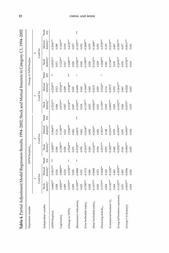
22 CHENG AND WEISSTable 4. Partia
l Adjustm
ent M
odel Regression Re
sults, 1994–2002; Stock and M
utua
l Insurers in Category C1, 1994–2002
Dep
ende
nt variable
(NPW
/Surplus) t+
1Cha
nge in N
PW/Surplus
12
34
Coeff for
Coeff for
Coeff for
Coeff for
Inde
pend
ent v
ariable
Stock
dummy*
Mutua
ldu
mmy*
Wald
test
Stock
dummy*
Mutua
ldu
mmy*
Wald
test
Stock
dummy*
Mutua
ldu
mmy*
Wald
test
Stock
dummy*
Mutua
ldu
mmy*
Wald
test
(NPW
/Surplus) t
0.6482***
0.7017***
***
0.4209***
0.3969***
–0.2532***
–0.2245***
**–0.4935***
–0.5546***
0.008
0.016
0.084
0.116
0.006
0.013
0.071
0.098
Log(Assets)
t0.0843***
0.0806***
0.1308***
0.1382***
0.0733***
0.0744***
0.1223***
0.1362***
0.009
0.010
0.020
0.021
0.007
0.009
0.017
0.018
(Cha
nge in N
PW) t
0.6370***
0.6728***
**0.5564***
0.5240***
0.5138***
0.5748***
***
0.4285***
0.4136***
0.009
0.026
0.031
0.062
0.007
0.022
0.026
0.053
(Reinsuran
ce utilization)
t–0.1509***
–0.0089
**–0.2729***
–0.0915
***
–0.1292***
–0.0459
*–0.2582***
–0.1355***
***
0.022
0.051
0.050
0.062
0.018
0.042
0.042
0.052
(Line herfinda
hl in
dex)
t–0.1585***
–0.1112
–0.2431***
–0.2164**
–0.1105***
–0.1669**
–0.1999***
–0.2808***
0.028
0.080
0.043
0.092
0.023
0.065
0.036
0.078
(State herfin
dahl in
dex)
t–0.1477***
–0.0908
–0.2126***
–0.2016**
–0.0943***
–0.0215
–0.1632***
–0.1408**
0.025
0.072
0.034
0.084
0.021
0.059
0.029
0.070
(Finan
cing deficit)
t+1
0.1773***
0.3430**
0.2571***
0.3817**
0.1195**
0.3322**
*0.2040***
0.3739***
0.064
0.142
0.072
0.148
0.052
0.116
0.061
0.125
(Com
mercial business %
) t–0.1143***
–0.1242**
–0.1807***
–0.2311***
–0.0833***
–0.0972*
–0.1534***
–0.2134***
0.064
0.063
0.042
0.079
0.025
0.052
0.035
0.067
(Lon
g‐tail bu
siness exp
osure)
t–0.1143***
–0.3078***
–0.2782***
–0.3976***
–0.1912***
–0.2616***
–0.2670***
–0.3587***
0.031
0.081
0.041
0.091
0.026
0.067
0.035
0.077
(Group (=
1) dum
my)
t–0.0633***
–0.0396
–0.0965***
–0.0933**
–0.0373**
–0.0228
–0.0724***
–0.0811***
0.019
0.028
0.023
0.036
0.015
0.023
0.019
0.031
RBC STRUCTURE 23
N15632
15458
15632
15458
Two‐stage‐least‐s
quares
No
Yes
No
Yes
C‐D wald F statistic
36.78
36.62
C‐D wald F statistic df
3,13356
3,13356
Sargan statistic
0.6770
3.1660
Sargan statistic P value
0.4107
0.0752
R‐squa
red
0.7452
0.4604
0.2795
0.3874
Note: Stan
dard Error app
ears below each coefficient. C‐D W
wald F statistic is th
e Cragg‐D
onald Wwald F statistic.
Note: ***significan
t at 1 percent level, **sign
ificant at 5 percent level, *significan
t at 1
0 pe
rcent level.
Note: All mod
els includ
e fix
ed com
pany and year e
ffects. Wald test is non
linear test tha
t βS=
β M.
Note: Lo
g(Assets) is th
e natural logarithm of total assets; chan
ge in NPW
is th
e growth in net premiums w
ritte
n; line and state h
erfin
dahl inde
xes a
re herfin
dahl inde
xes o
f premiums
writte
n by produ
ct line and by state, re
spectiv
ely; fina
ncing de
ficit is (cha
nge in working cap
ital m
inus lagg
ed cash flo
w from ope
ratio
ns) d
ivided by assets; com
mercial business
% is th
e prop
ortio
n of net premiums writte
n in com
mercial lines; lo
ng‐ta
il bu
siness exp
osure is th
e ratio of insuran
ce re
serves to lo
sses in
curred in th
e current y
ear; an
d grou
p is
a du
mmy variable equ
al to one if th
e insurer is a mem
ber o
f a group
, and zero otherw
ise.
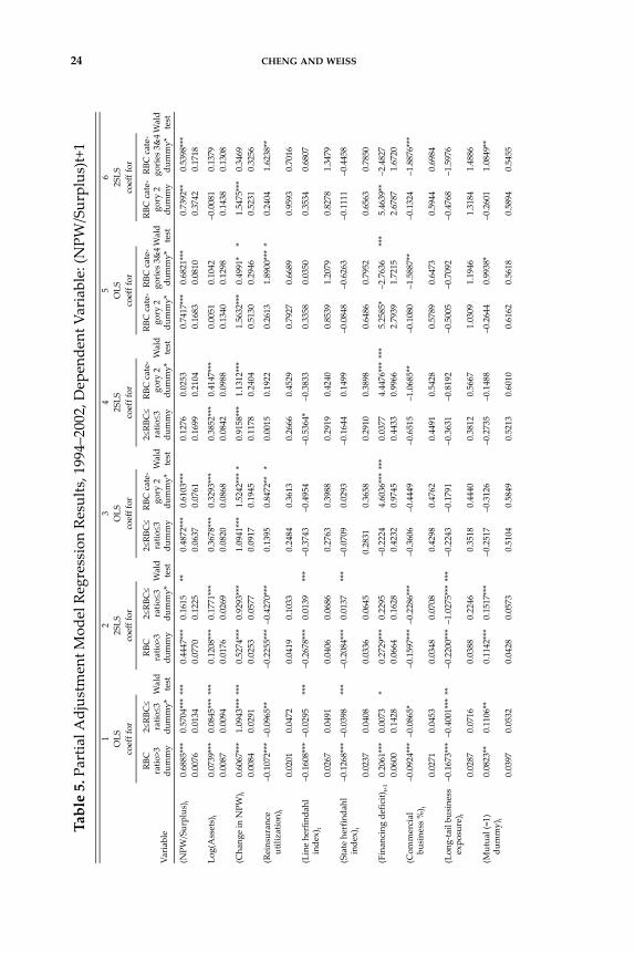
24 CHENG AND WEISSTable 5. Partia
l Adjustm
ent M
odel Regression Results, 1994–2002, D
epende
nt Variable: (N
PW/Surplus)t+
1
12
34
56
OLS
2SLS
OLS
2SLS
OLS
2SLS
coeff for
coeff for
coeff for
coeff for
coeff for
coeff for
RBC
ratio
>3du
mmy
2≤RB
C≤
ratio
≤3du
mmy*
Wald
test
RBC
ratio
>3
dummy
2≤RB
C≤
ratio
≤3
dummy*
Wald
test
2≤RB
C≤
ratio
≤3
dummy
RBC cate‐
gory 2
dummy*
Wald
test
2≤RB
C≤
ratio
≤3du
mmy
RBC cate‐
gory 2
dummy*
Wald
test
RBC cate‐
gory 2
dummy*
RBC cate‐
gories 3&4
dummy*
Wald
test
RBC cate‐
gory 2
dummy
RBC cate‐
gories 3&4
dummy*
Wald
test
Variable
(NPW
/Surplus) t
0.6885***
0.5704******
0.4447***
0.1615
**0.4872***
0.6103***
0.1276
0.0253
0.7417***
0.6821***
0.7392**
0.5398***
0.0076
0.0134
0.0770
0.1225
0.0637
0.0761
0.1699
0.2104
0.1683
0.0810
0.3742
0.1718
Log(Assets)
t0.0739***
0.0845******
0.1208***
0.1771***
0.3678***
0.3293***
0.3852***
0.4147***
0.0051
0.1042
–0.0081
0.1379
0.0087
0.0094
0.0176
0.0269
0.0820
0.0868
0.0842
0.0988
0.1340
0.1298
0.1438
0.1308
(Cha
nge in N
PW) t
0.6067***
1.0943******
0.5274***
0.9293***
1.0941***
1.5242****
0.9158***
1.1312***
1.5632***
0.4991*
*1.5475***
0.3469
0.0084
0.0291
0.0253
0.0577
0.0917
0.1945
0.1178
0.2404
0.5130
0.2946
0.5231
0.3256
(Reinsuran
ce
utilizatio
n)t
–0.1072***
–0.0965**
–0.2255***
–0.4270***
0.1395
0.8472**
*0.0015
0.1922
0.2613
1.8900****
0.2404
1.6238**
0.0201
0.0472
0.0419
0.1033
0.2484
0.3613
0.2666
0.4529
0.7927
0.6689
0.9593
0.7016
(Line herfinda
hl
inde
x)t
–0.1608***
–0.0295
***
–0.2678***
0.0139
***
–0.3743
–0.4954
–0.5364*
–0.3833
0.3358
0.0350
0.3534
0.6807
0.0267
0.0491
0.0406
0.0686
0.2763
0.3988
0.2919
0.4240
0.8539
1.2079
0.8278
1.3479
(State herfin
dahl
inde
x)t
–0.1268***
–0.0398
***
–0.2084***
0.0137
***
–0.0709
0.0293
–0.1644
0.1499
–0.0848
–0.6263
–0.1111
–0.4458
0.0237
0.0408
0.0336
0.0645
0.2831
0.3658
0.2910
0.3898
0.6486
0.7952
0.6563
0.7850
(Finan
cing deficit)
t+1
0.2061***
0.0073
*0.2729***
0.2295
–0.2224
4.6036******
0.0377
4.4476******
5.2585*
–2.7636
***
5.4639**
–2.4827
0.0600
0.1428
0.0664
0.1628
0.4232
0.9745
0.4433
0.9966
2.7939
1.7215
2.6787
1.6720
(Com
mercial
business %
) t–0.0924***
–0.0865*
–0.1597***
–0.2286***
–0.3606
–0.4449
–0.6515
–1.0685**
–0.1080
–1.5887**
–0.1324
–1.8876***
0.0271
0.0453
0.0348
0.0708
0.4298
0.4762
0.4491
0.5428
0.5789
0.6473
0.5944
0.6984
(Lon
g‐tail bu
siness
expo
sure) t
–0.1673***
–0.4001***
**–0.2200***
–1.0275***
***
–0.2243
–0.1791
–0.3631
–0.8192
–0.5005
–0.7092
–0.4768
–1.5976
0.0287
0.0716
0.0388
0.2246
0.3518
0.4440
0.3812
0.5667
1.0309
1.1946
1.3184
1.4886
(Mutua
l (=1)
dummy)
t
0.0823**
0.1106**
0.1142***
0.1517***
–0.2517
–0.3126
–0.2735
–0.1488
–0.2644
0.9938*
–0.2601
1.0849**
0.0397
0.0532
0.0428
0.0573
0.5104
0.5849
0.5213
0.6010
0.6162
0.5618
0.5894
0.5455
RBC STRUCTURE 25
(Other org. form (=1)
dummy ) t
–0.0138
–0.0846
–0.0542
–0.1037
*0.6021
1.1146
*0.7519
1.0397
–0.1133
–0.9525
*–0.1003
–1.0483
0.0451
0.0581
0.0493
0.0628
0.8012
0.8266
0.8214
0.8457
0.6104
0.7217
0.5834
0.6973
(Group (=
1)
dummy)
t
–0.0439***
–0.1155***
*–0.0692***
–0.2001***
***
0.0405
–0.0211
0.0466
–0.1316
0.1165
–1.2876**
0.1189
–1.3774**
0.0148
0.0296
0.0175
0.0424
0.1530
0.2280
0.1585
0.2408
0.4763
0.6134
0.4684
0.5938
N16916
16714
1370
1120
353
353
Fixed compa
ny
effects
Yes
Yes
Yes
Yes
No
No
Two‐stage‐least
squa
res
No
Yes
No
Yes
No
Yes
C‐D wald F statistic
46.9
38.31
23.41
C‐D wald F statistic
df3,14427
3,734
4,317
Sargan statistic
1.983
0.089
0.001
R‐squa
red
0.7601
0.4603
0.1662
0.2518
0.4252
0.4196
Note: Stan
dard Error app
ears below each coefficient. C‐D wald F statistic is th
e Cragg‐D
onald wald F statistic. A
ll mod
els includ
e fix
ed year e
ffects. W
ald test is non
linear test tha
t βS=
β M.
Note: *** significan
t at 1 percent level, ** signific
ant a
t 5% level, an
d * significan
t at 1% level.
Note: Lo
g(Assets) is th
e na
tural log
arith
m of total assets; chan
ge in N
PW is th
e grow
th in net premiums w
ritte
n; line and state herfin
dahl in
dexes a
re herfin
dahl in
dexes o
f premiums writte
n by produ
ct line and by state, re
spectiv
ely; fina
ncing de
ficit is (cha
nge in working cap
ital m
inus lagg
ed cash flo
w from ope
ratio
ns) d
ivided by assets; com
mercial business % is th
e prop
ortio
n of net premiums w
ritte
n in com
mercial lines; lo
ng‐ta
il bu
siness exp
osure is th
e ratio of insuran
ce re
serves to lo
sses in
curred in th
e current y
ear; grou
p (m
utua
l) is a dum
my variable equ
al to
one if the insurer is a m
ember o
f a group (is a m
utua
l), and zero otherw
ise; and other org. form is a dum
my variable equ
al to one if th
e insurer is n
either a stock no
r a m
utua
l insurer.
26 CHENG AND WEISSTable 6. Partia
l Adjustm
ent R
egression Re
sults, 1994–2002
NAIC RBC category C1
RBC Ratio > 3
Dep
ende
nt variable
Cha
nge in (L
iabilities/Assets)
(Liabilities/Assets)
t+1
Cha
nge in (L
iabilities/Assets)
(Liabilities/Assets)
t+1
(1)
(2)
(3)
(4)
(5)
(6)
(7)
(8)
Inde
pend
ent v
ariables
Coeff.
Coeff.
Coeff.
Coeff.
Coeff.
Coeff.
Coeff.
Coeff.
(Liabilities/Assets)
t –0.2029***
–0.1439***
0.6667***
0.7882***
–0.1969***
–0.1151***
0.6659***
0.7571***
0.0049
0.0083
0.0067
0.0113
0.0052
0.0100
0.0071
0.0136
Log(Assets)
t0.0069***
0.0011
0.0092***
–0.0027
0.0072***
–0.0013
0.0100***
0.0005
0.0014
0.0016
0.0019
0.0021
0.0015
0.0018
0.0021
0.0024
(Cha
nge in N
PW) t
0.0525***
0.0557***
0.0669***
0.0735***
0.0547***
0.0586***
0.0708***
0.0753***
0.0013
0.0013
0.0017
0.0018
0.0013
0.0014
0.0018
0.0019
(Reinsuran
ce utilization)
t–0.0112***
–0.0091***
–0.0106**
–0.0062
–0.0133***
–0.0107***
–0.0136***
–0.0106**
0.0031
0.0031
0.0042
0.0042
0.0032
0.0032
0.0044
0.0044
(Line herfinda
hl in
dex)
t–0.0263***
–0.0213***
–0.0270***
–0.0167***
–0.0282***
–0.0208***
–0.0297***
–0.0214***
0.0042
0.0042
0.0056
0.0057
0.0043
0.0044
0.0059
0.0060
(State herfin
dahl in
dex)
t–0.0241***
–0.0207***
–0.0358***
–0.0289***
–0.0229***
–0.0183***
–0.0359***
–0.0307***
0.0037
0.0037
0.0050
0.0051
0.0038
0.0039
0.0052
0.0053
(Finan
cing deficit)
t+1
0.0894***
0.0899***
0.1178***
0.1188***
0.0977***
0.0982***
0.1264***
0.1270***
0.0087
0.0088
0.0118
0.0120
0.0094
0.0095
0.0129
0.0129
(Com
mercial business %) t
–0.0147***
–0.0137***
–0.0251***
–0.0229***
–0.0158***
–0.0144***
–0.0270***
–0.0255***
0.0042
0.0043
0.0057
0.0058
0.0043
0.0044
0.0060
0.0060
(Lon
g‐tail bu
siness exp
osure)
t–0.0063
–0.0074*
0.0007
–0.0015
–0.0088*
–0.0105**
–0.0057
–0.0076
0.0045
0.0045
0.0060
0.0061
0.0046
0.0046
0.0062
0.0063
(Mutua
l (=1) d
ummy)
t0.0165***
0.0155**
0.0222***
0.0203**
0.0173***
0.0159**
0.0224***
0.0209**
0.0062
0.0063
0.0084
0.0085
0.0064
0.0064
0.0087
0.0088

RBC STRUCTURE 27
(Other org. form (=
1) dum
my ) t
–0.0035
–0.0029
–0.0094
–0.0083
–0.0029
–0.0020
–0.0111
–0.0101
0.0071
0.0071
0.0096
0.0097
0.0072
0.0073
0.0099
0.0100
(Group (=
1) dum
my)
t–0.0003
0.0007
–0.0007
0.0014
–0.0006
0.0007
–0.0008
0.0006
0.0023
0.0023
0.0031
0.0031
0.0024
0.0024
0.0033
0.0033
N16916
16916
16916
16916
15750
15750
15750
15750
Two‐stage‐Le
ast‐s
quares
No
Yes
No
Yes
No
Yes
No
Yes
C‐D wald F statistic
4008.75
4008.75
2509.99
2509.99
C‐D wald F statistic df
2,14439
2,14439
2,133313
2,13313
Sargan statistic
0.6370
0.2220
0.4230
0.0440
Sargan statistic P value
0.4248
0.6372
0.5155
0.8342
R‐squ
ared
0.1527
0.1947
0.8214
0.8471
0.1563
0.2153
0.8173
0.8414
Note: Stan
dard Error app
ears below each coeffic
ient. C‐D wald F Sstatistic is th
e Cragg‐D
onald wald F statistic. A
ll mod
els includ
e fix
ed com
pany and year e
ffects.
Note: *** significan
t at 1 percent level, ** signific
ant a
t 5% level, an
d * s
ignific
ant a
t 1% level.
Note: Th
e RB
C ra
tio is defined as the ra
tio of total adjusted capital to au
thorized co
ntrol level RBC
; Log
(Assets) is th
e na
tural log
arith
m of total assets; ch
ange in NPW
is th
e grow
th in net premiums writte
n; line and state H
erfin
dahl in
dexes are herfinda
hl in
dexes of premiums writte
n by produ
ct line and by state, respe
ctively;
finan
cing deficit is (cha
nge in working cap
ital m
inus lagg
ed cash flo
w from ope
ratio
ns) d
ivided by assets; com
mercial business % is th
e prop
ortio
n of net premiums
writte
n in com
mercial lines; lo
ng‐ta
il bu
siness exp
osure is th
e ratio of insuran
ce re
serves to lo
sses in
curred in th
e current y
ear; grou
p (m
utua
l) is a dum
my variable
equa
l to on
e if the insurer is a mem
ber o
f a group (is a mutua
l), and zero otherw
ise; and other org. form is a dum
my variable equ
al to one if th
e insurer is neith
er a
stock no
r a m
utua
l insurer.

28 CHENG AND WEISSTable 7. Partia
l Adjustm
ent M
odel Regression Re
sults, 1994–2002;
Stock an
d Mutua
l Insurers in Category C1, 1994–2002
Dep
ende
nt variable
(Liabilities/Assets)
t+1
Cha
nge in Liabilities/Assets
12
34
Coeff for
Coeff for
Coeff for
Coeff for
Variable
Stock
dummy*
Mutua
ldu
mmy*
Wald
test
Stock
dummy*
Mutua
ldu
mmy*
Wald
test
Stock
dummy*
Mutua
ldu
mmy*
Wald
test
Stock
dummy*
Mutua
ldu
mmy*
Wald
test
(Liabilities/Assets)
t 0.6610***
0.7272***
***
0.6583***
0.6174***
–0.2051***
–0.1806***
*–0.2463***
–0.2998***
0.007
0.018
0.046
0.087
0.005
0.013
0.034
0.066
Log(Assets )t
0.0110***
0.0089***
0.0111**
0.0131**
0.0075***
0.0077***
0.0115***
0.0145***
0.002
0.002
0.005
0.005
0.001
0.002
0.004
0.004
(Cha
nge in N
PW) t
0.0674***
0.0630***
**0.0672***
0.0562***
0.0521***
0.0576***
0.0498***
0.0504***
0.002
0.005
0.003
0.007
0.001
0.004
0.002
0.006
(Reinsuran
ce utilization)
t–0.0120***
–0.0042
–0.0121**
–0.0038
–0.0133***
0.0017
*–0.0151***
0.0024
**0.005
0.011
0.005
0.011
0.003
0.008
0.004
0.008
(Line herfinda
hl in
dex)
t–0.0246***
–0.0190
–0.0250***
–0.0264
–0.0244***
–0.0302**
–0.0281***
–0.0374***
0.006
0.017
0.007
0.018
0.004
0.012
0.005
0.013
(State herfin
dahl in
dex)
t–0.0381***
–0.0128
–0.0385***
–0.0198
–0.0244***
–0.0170
–0.0270***
–0.0243**
0.005
0.015
0.006
0.016
0.004
0.011
0.004
0.012
(Finan
cing deficit)
t+1
0.1246***
0.0958***
0.1254***
0.0890***
0.0975***
0.0622***
0.0983***
0.0556**
*0.013
0.030
0.013
0.030
0.010
0.022
0.010
0.022
(Com
mercial business %) t
–0.0288***
–0.0439***
–0.0288***
–0.0468***
–0.0137***
–0.0405***
***
–0.0145***
–0.0435***
***
0.007
0.013
0.007
0.013
0.005
0.010
0.005
0.010
(Lon
g‐tail bu
siness
expo
sure) t
0.0024
0.0021
0.0014
0.0107
–0.0059
–0.0014
–0.0059
0.0069
0.007
0.017
0.007
0.018
0.005
0.013
0.005
0.014
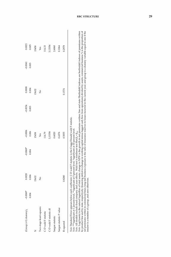
RBC STRUCTURE 29
(Group (=
1) dum
my)
t–0.0069*
0.0020
–0.0069*
–0.0006
–0.0034
0.0008
–0.0041
0.0021
0.004
0.006
0.004
0.006
0.003
0.004
0.003
0.005
N15632
15458
15632
15458
Two‐stage‐least‐s
quares
No
Yes
No
Yes
C‐D wald F statistic
114.79
114.33
C‐D wald F statistic df
3,13356
3,13356
Sargan statistic
0.6020
2.6060
Sargan statistic P value
0.4376
0.1064
R‐squa
red
0.8280
0.5055
0.1574
0.2978
Note: Stan
dard Error app
ears below each coefficient. C‐D wald F statistic is th
e Cragg‐D
onald wald F statistic.
Note: ***signific
ant a
t 1 percent level, **sign
ificant at 5 percent level, *significan
t at 1
0 pe
rcent level.
Note: All mod
els includ
e fix
ed com
pany and year e
ffects. W
ald test is non
linear test tha
t βS =
β M.
Note: Lo
g(Assets) is th
e na
tural log
arith
m of total assets; chan
ge in N
PW is th
e grow
th in net premiums writte
n; line and state H
erfin
dahl in
dexes are herfinda
hl in
dexes of premiums writte
nby produ
ct line and by state, re
spectiv
ely; fina
ncing de
ficit is (cha
nge in working cap
ital m
inus lagg
ed cash flo
w from ope
ratio
ns) d
ivided by assets; com
mercial business % is th
e prop
ortio
n of
net p
remiums w
ritte
n in com
mercial lines; lo
ng‐ta
il bu
siness exp
osure is th
e ratio of insuran
ce re
serves to lo
sses in
curred in th
e current y
ear; an
d grou
p is a dum
my variable equ
al to one if th
einsurer is a m
ember o
f a group
, and zero otherw
ise.
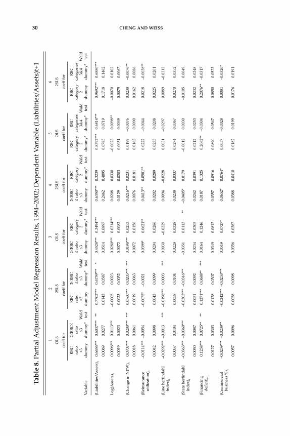
30 CHENG AND WEISSTable 8. Partia
l Adjustm
ent M
odel Regression Results, 1994–2002; D
epende
nt Variable (Liabilities/Assets)t+1
1
23
45
6OLS
2SLS
OLS
2SLS
OLS
2SLS
coeff for
coeff for
coeff for
coeff for
coeff for
coeff for
Variable
RBC
ratio >3
dummy
2≤RB
C≤
ratio ≤3
dummy*
Wald
test
RBC
ratio >3
dummy
2≤RB
C≤ratio
≤3du
mmy*
Wald
test
2≤RB
C≤ ratio
≤3du
mmy
RBC
catego
ry
2du
mmy*
Wald
test
2≤RB
C≤ ratio
≤3du
mmy
RBC
catego
ry
2du
mmy*
Wald
test
RBC
catego
ry
2du
mmy*
RBC
catego
ries
3&4
dummy*
Wald
test
RBC
catego
ry
2du
mmy
RBC
catego
ries
3&4
dummy*
Wald
test
(Liabilities/Assets)
t 0.6656***
0.6037***
**0.7702***
0.6759***
*0.4528***
0.3494***
0.6350***
0.3239
0.8392***
0.6814***
0.9692***
0.6880***
0.0069
0.0277
0.0143
0.0587
0.0514
0.0897
0.2462
0.4095
0.0785
0.0719
0.1718
0.1462
Log(Assets)
t0.0096***
0.0113***
–0.0005
0.0023
0.0280***
0.0314***
0.0208
0.0330
–0.0023
0.0098**
–0.0070
0.0102
0.0019
0.0023
0.0023
0.0032
0.0072
0.0082
0.0129
0.0203
0.0051
0.0049
0.0075
0.0067
(Cha
nge in N
PW) t
0.0707***
0.0200***
***
0.0760***
0.0205***
***
0.0198***
0.0253
0.0216***
0.0231
0.0199
–0.0076
0.0238
–0.0076**
0.0018
0.0061
0.0019
0.0063
0.0072
0.0156
0.0076
0.0181
0.0163
0.0090
0.0162
0.0086
(Reinsuran
ce
utilizatio
n)t
–0.0114***
–0.0054
–0.0075*
–0.0021
0.0399*
0.0621**
0.0413**
0.0581**
0.0222
–0.0044
0.0218
–0.0038**
0.0042
0.0098
0.0043
0.0099
0.0204
0.0286
0.0202
0.0289
0.0235
0.0208
0.0225
0.0201
(Line herfinda
hl
inde
x)t
–0.0292***
–0.0013
***
–0.0198***
0.0003
***
0.0030
–0.0229
0.0094
–0.0228
0.0031
–0.0297
0.0089
–0.0313
0.0057
0.0104
0.0058
0.0104
0.0228
0.0328
0.0238
0.0337
0.0274
0.0367
0.0270
0.0352
(State herfin
dahl
inde
x)t
–0.0363***
–0.0360***
–0.0303***
–0.0316***
–0.0351
0.0113
**–0.0405*
0.0179
–0.0012
0.0030
–0.0105
0.0049
0.0050
0.0087
0.0051
0.0092
0.0234
0.0305
0.0242
0.0391
0.0212
0.0253
0.0232
0.0248
(Finan
cing
defic
it)t+1
0.1258***
0.0725**
**0.1271***
0.0688**
***
0.0164
0.1246
0.0187
0.1325
0.2062**
–0.0304
0.2076**
–0.0317
0.0127
0.0303
0.0128
0.0307
0.0349
0.0812
0.0357
0.0916
0.0890
0.0547
0.0850
0.0523
(Com
mercial
business %
) t–0.0259***
–0.0239**
–0.0242***
–0.0253***
0.0519
0.0727*
0.0652*
0.0764*
0.0057
–0.0328
0.0081
–0.0320*
0.0057
0.0096
0.0058
0.0098
0.0356
0.0387
0.0388
0.0410
0.0182
0.0199
0.0176
0.0191
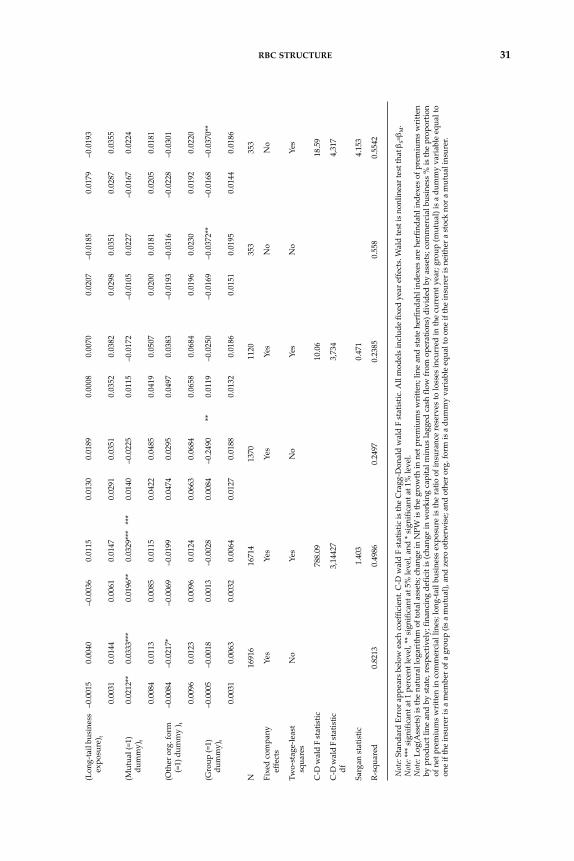
RBC STRUCTURE 31
(Lon
g‐tail bu
siness
expo
sure) t
–0.0015
0.0040
–0.0036
0.0115
0.0130
0.0189
0.0008
0.0070
0.0207
–0.0185
0.0179
–0.0193
0.0031
0.0144
0.0061
0.0147
0.0291
0.0351
0.0352
0.0382
0.0298
0.0351
0.0287
0.0355
(Mutua
l (=1)
dummy)
t
0.0212**
0.0333***
0.0196**
0.0329***
***
0.0140
–0.0225
0.0115
–0.0172
–0.0105
0.0227
–0.0167
0.0224
0.0084
0.0113
0.0085
0.0115
0.0422
0.0485
0.0419
0.0507
0.0200
0.0181
0.0205
0.0181
(Other org. form
(=1) dum
my ) t
–0.0084
–0.0217*
–0.0069
–0.0199
0.0474
0.0295
0.0497
0.0383
–0.0193
–0.0316
–0.0228
–0.0301
0.0096
0.0123
0.0096
0.0124
0.0663
0.0684
0.0658
0.0684
0.0196
0.0230
0.0192
0.0220
(Group (=
1)
dummy)
t
–0.0005
–0.0018
0.0013
–0.0028
0.0084
–0.2490
**0.0119
–0.0250
–0.0169
–0.0372**
–0.0168
–0.0370**
0.0031
0.0063
0.0032
0.0064
0.0127
0.0188
0.0132
0.0186
0.0151
0.0195
0.0144
0.0186
N16916
16714
1370
1120
353
353
Fixed compa
ny
effects
Yes
Yes
Yes
Yes
No
No
Two‐stage‐least
squa
res
No
Yes
No
Yes
No
Yes
C‐D wald F statistic
788.09
10.06
18.59
C‐D wald F statistic
df3,14427
3,734
4,317
Sargan statistic
1.403
0.471
4.153
R‐squa
red
0.8213
0.4986
0.2497
0.2385
0.558
0.5542
Note: Stan
dard Error app
ears below each coefficient. C‐D wald F statistic is th
e Cragg‐D
onald wald F statistic. A
ll mod
els includ
e fix
ed year e
ffects. W
ald test is non
linear test tha
t βS=
β M.
Note: *** significan
t at 1 percent level, ** signific
ant a
t 5% level, an
d * significan
t at 1% level.
Note: Lo
g(Assets) is th
e na
tural log
arith
m of total assets; cha
nge in N
PW is th
e grow
th in net premiums writte
n; line and state herfin
dahl in
dexes are herfinda
hl in
dexes of premiums writte
nby produ
ct line and by state, re
spectiv
ely; fina
ncing de
ficit is (cha
nge in w
orking cap
ital m
inus lagg
ed cash flo
w from ope
ratio
ns) d
ivided by assets; com
mercial business % is th
e prop
ortio
nof net premiums writte
n in com
mercial lines; lo
ng‐ta
il bu
siness exp
osure is th
e ratio of insuran
ce re
serves to lo
sses in
curred in th
e current y
ear; grou
p (m
utua
l) is a dum
my variable equ
al to
one if the insurer is a m
ember o
f a group (is a m
utua
l), and zero otherw
ise; and other org. form is a dum
my variable equ
al to one if th
e insurer is n
either a stock no
r a m
utua
l insurer.
32 CHENG AND WEISS
sample.26 Hausman tests indicated that fixed company effects were favoredover random effects in the panel data models. Fixed time effects areincluded in each model. OLS and instrumental variables (2SLS) models areprovided in each table for comparison purposes. In the instrumentalvariables models, the Cragg‐Donald partial F statistics (weak instrumentstest) are provided as well as the Sargan statistics (test of the validity of theinstruments). The results of these two tests indicate that the instrumentsused are valid (i.e., the Sargan statistics are insignificant at the 5 percentlevel or better), and that they pass the weak instruments test, with limitedexceptions.27
Relative Importance of Tradeoff and Pecking Order Theory
Hypothesis 1 states that the tradeoff theory dominates the peckingorder theory in explaining insurer capital structure. For reasons explainedearlier, this hypothesis is tested using well‐capitalized insurers, defined inthis study as insurers in category C1. Regressions using the change in(NPW/Surplus) and change in (Liabilities/Assets) (eq. (7)) and (NPW/Surplus)t+1 and (Liabilities/Assets)t+1 (eq. (3)) are used to test this hypothe‐sis, and the regression results are presented in Tables 3 and 6. Results areincluded also for insurers that have RBC ratios significantly above the C1threshold level (i.e., RBC ratios > 3).
The results for the models in Table 3 using (NPW/Surplus)t+1 as thedependent variable (columns 3–4 and 7–8) support the tradeoff theory inthat the coefficients for the lagged (NPW/Surplus) are positive and signif‐icant for all models. The adjustment speed associated with the 2SLS coef‐ficients for categories C1 and for insurers with an RBC ratio > 3 imply thatinsurers adjust toward their optimal target ratio at a rate of approximately25 to 35 percent per year (i.e., δ ranges from 1–0.7525 to 1–0.6504). However,the coefficients for the financing deficit variables are positive and signifi‐cant, suggesting that financial slack is related to capital structure also.
To determine whether the tradeoff theory is dominant, regressionresults with the change in (NPW/Surplus) as the dependent variable andthe lagged (NPW/Surplus) and financing deficit variables as independentvariables are evaluated. (See columns 1–2 and 5–6 in Table 3.) Note that the
26Panel methods are used for insurers with RBC ratios > 3 and for insurers with 2 ≤ RBC ratio≤ 3. In the other samples, insurers had a tendency to move into a different category from oneyear to the next, so that panel data methods could not be used.27The exceptions are in Tables 5 and 8 when comparisons of insurers in categories C2 andC3–C4 are made. Therefore, separate regressions are run for insurers in categories C2 andC3–C4, and a comparison of the coefficients of the leverage ratios is made. The results donot change.

RBC STRUCTURE 33
sign and significance of the coefficient for (NPW/Surplus)t is still negativeand significant at better than the 1 percent level in the change in (NPW/Surplus) equations in Table 3,28 but the implied adjustment speed issmaller, varying from 17.28 to 25.49 percent across the different categoriesshown. However, the positive and significant coefficients for the financingdeficit variable in Table 3 are consistent with the pecking order theory.
The economic impact of the (NPW/Surplus) and financing deficitvariables in the change in (NPW/Surplus) regressions are used to deter‐mine the relative importance of the pecking order and tradeoff theories.29The economic impact of a one‐standard‐deviation change in the (NPW/Surplus) and financing deficit variables in the 2SLS results for insurers incategory C1 (with RBC ratios > 3) are 38.9 (38.8) and 2.3 (3.8) percents,respectively. Results are similar when the OLS coefficients are used. Thusan increase of one standard deviation in (NPW/Surplus) would have asignificantly larger effect on the change in (NPW/Surplus) than an increaseof one standard deviation for the financing deficit variable. On balance,then, it appears that the tradeoff theory is more important than the peckingorder theory, since the financing deficit variable does not wipe out the effectof the other variables in the ∆(Capital ratio)i,t+1 equations. Thus Hypothesis1 is supported in the (NPW/Surplus) regressions.
Table 6 has the same models as in Table 3 except that the leverage ratiois (Liabilities/Assets). Hypothesis 1 is supported by the results in Table 6since the coefficients for lagged (Liabilities/Assets) are positive and signif‐icant in the (Liabilities/Assets)t+1 models and negative and significant in thechange in (Liabilities/Assets) models. The speed of adjustment impliedfrom the (Liabilities/Assets)t+1 models ranges from (1–.6667) to (1–.7882),according to Table 6. The speed of adjustment appears to be somewhatlower in the change in (Liabilities/Assets) equation, ranging from 11.59 to20.29 percents.
The coefficients for both the financing deficit and lagged (Liabilities/Assets) variables are significant in the change in (Liabilities/Assets) regres‐
28Recall that in the change in leverage ratio equation (eq. (7)), (leverage ratio)t is subtracted.29The economic significance of (NPW/Surplus) in the equations is determined by finding theeffect of a one‐standard‐deviation change in the target (NPW/Surplus) ratio and the finan‐cial slack variable on the fitted value of the change in (NPW/Surplus) (i.e., predicted∆(NPW/Surplus))t+1). The target (NPW/Surplus) is found using equation (1). The economicimpact of a one‐standard‐deviation change in (NPW/Surplus) is computed as (coefficient forlagged (NPW/Surplus) * standard deviation of target (NPW/Surplus))/(standard deviationof the fitted value for change in (NPW/Surplus)); and the economic impact of the financingdeficit variable is found by calculating (coefficient for financing deficit * standard deviationof financing deficit variable)/(standard deviation of fitted value for change in the target(NPW/Surplus)). This approach is used in Flannery and Rangan (2006) as well.
34 CHENG AND WEISS
sions, and the economic impact of a one‐standard‐deviation change in the(Liabilities/Assets) and financing deficit variables are 47.8 (49.1) and 9.5(12.1) percents, respectively, for insurers in category C1 (with RBC ratio >3). Thus, like the results in Table 3, the dominance of the tradeoff theoryover the pecking order theory is supported.
Mutual versus Stock Insurer Results
Hypothesis 1a indicates that mutual and stock insurers do not havethe same target capital level. This hypothesis is tested by comparing thecoefficients of the independent variables (βM and βS) interacted with thestock and mutual dummies by means of a nonlinear wald test. The overallregression results are presented in Table 4.30 The coefficients for the inter‐action of the stock dummy and the independent variables are shown in onecolumn for each equation (i.e., DS[ (δSβS)XSit + (1 – δS) (Capital ratio)Sit]) andthe coefficients for the interaction of the mutual dummy with the indepen‐dent variables are shown in the adjacent column (i.e., DM [ (δMβM)XMit + (1– δM) (Capital ratio)Mit]). The sample of insurers in category C1 is used forthis test, because the RBC ratio adjustment speed should be affected if theinsurer is experiencing financial distress, and stocks are more likely tobecome insolvent (Cummins, Harrington, and Klein, 1995; Cummins,Grace, and Phillips, 1999).
Recall that if any of the coefficients for the mutual interaction dummyvariables XM are significantly different from the stock interaction terms (i.e.,elements of βS not equal to βM), it would signify that the target RBC ratiovaries between stock and mutual insurers with respect to that factor. Thenonlinear wald test results in Table 4 indicate that the coefficients for(NPW/Surplus)t are significantly different for stocks versus mutuals in allresults except for 2SLS results for (NPW/Surplus)t+1. According to the waldtests in Table 4, the coefficients for (Reinsurance utilization)t are signifi‐cantly different between stock and mutual insurers in all models, while thecoefficients (Change in NPW)t are significantly different between stocksand mutuals in some models. Overall, these results support Hypothesis 1a,which states that mutual and stock insurers do not have the same targetcapital level. This is consistent with Harrington and Niehaus (2002), whofind evidence that capital to liability ratios differ between stock and mutualinsurers.31
30Evidence to support this hypothesis can also be found in Tables 3 and 6. The coefficientsfor the mutual dummy variables are positive and significant in the (NPW/Surplus)t+1 and(Liabilities/Assets)t+1 regressions in Tables 3 and 6. 31However, Harrington and Niehaus (2002) find that mutual insurers hold more capital thanstock insurers.
RBC STRUCTURE 35
Two of the four models reported in Table 7 indicate that mutuals havesignificantly different (Liabilities/Assets) than stock insurers because waldtests indicate significant differences in some βM compared to βS in thesemodels (i.e., models 1 and 3). Also, the coefficients for (Reinsurance Utili‐zation)t and (Commercial business %)t are significantly different for stockversus mutuals in the results in Table 7 for change in (Liabilities/Assets).Thus, overall, the results in Table 7 mostly support the hypothesis ofdifferent target leverage ratios for stocks versus mutuals.
Hypothesis 1b indicates that mutuals adjust toward their target lever‐age ratio more slowly than stock insurers. Hypothesis 1b would be sup‐ported if the coefficient for (NPW/Surplus)t is larger and significantlydifferent than for stock insurers in Table 4. The 2SLS results in models 2and 4 in Table 4 indicate that the adjustment speed for mutual insurers andstock insurers are not significantly different, since the wald test result isnot significant. Significant differences in the coefficients for (NPW/Sur‐plus)t in the OLS results exist, however. The OLS results in columns 1 and3 indicate that mutuals’ adjustment speed is slower than for stocks,although the differences are not large. For example, in model 1, the adjust‐ment speeds for mutual versus stock insurers are, respectively, (1–.7017)and (1–.6482), while the adjustment speed is 22.45 and 25.32 percents,respectively, in model 3 in Table 5. The OLS results are consistent withHarrington and Niehaus (2002). Thus, limited evidence exists that mutualsadjust their capital structure more slowly than stock insurers.
The OLS regressions in model 1 in Table 7 indicate that mutuals adjustsignificantly more slowly to the target (Liabilities/Assets) level than stockinsurers, with adjustment speeds of (1–.7272) for mutuals versus (1–.6610)for stock insurers. As in Table 4, no significant differences exist in adjust‐ment speeds in the 2SLS models in Table 7 in columns 2 and 4. Thus, onceagain, only limited evidence exists that mutuals adjust their capital struc‐ture more slowly than stock insurers.
Hypothesis 1d states that mutuals should be more sensitive to financ‐ing deficits than stock insurers. If mutuals are more sensitive to financingdeficits, then the coefficient for the financing deficit variable interactedwith the mutual dummy variable should be significantly larger in thechange in (NPW/Surplus) equations in Table 4. The results in the changein (NPW/Surplus) regressions in Table 4 (models 3 and 4) indicate that thefinancing deficit is positively related to the change in (NPW/Surplus)t+1, asexpected. However, the wald test for differences in the coefficients for stockand mutual insurers indicates that the differences in the coefficientsbetween stock and mutual insurers are not significant except in one case,where it is significant at the 10 percent level.32 Thus, Hypothesis 1d is notsupported.33, 34
36 CHENG AND WEISS
The results in Table 7 do not support Hypothesis 1d, either, since thewald tests for differences in the coefficients of the stock and dummyinteractions with the financing deficit variable are insignificant except inone case. The exception occurs in the 2SLS results for model 4, where thewald test statistic is significant at the 10 percent level. But the coefficientfor the interaction of the mutual dummy variable with the financing deficitvariable is smaller than the interaction for the stock dummy variable,contrary to Hypothesis 1d.
Long-Tail Business and Capital Structure
Hypothesis 1c indicates that insurers that write relatively more long‐tail lines have lower target capital levels. The results in Tables 3 and 4 showthat the coefficients for the long‐tail business exposure variable, (Long‐TailBusiness Exposure), in the (NPW/Surplus) regressions are significant andnegative in all models, as expected. Thus, insurers with more long‐tailbusiness exposure appear to operate with lower (NPW/Surplus). However,the same results do not hold for the (Liabilities/Assets) results. That is, inTables 6 and 7, the coefficients for the (Long‐Tail Business Exposure)variable are generally not significant. Therefore, mixed results exist forHypothesis 1c.
Financial Condition and Speed of Adjustment
To determine whether insurers in relatively worse financial conditionadjust towards their optimal capital RBC ratios at faster speeds, equation(6) is estimated for several samples of insurers. The results are presentedin Table 5 for (NPW/Surplus) and in Table 8 for (Liabilities/Assets). Ifinsurers in relatively worse financial condition adjust more quicklytowards their target capital ratio, then the coefficients for the interaction ofthe Cp dummy with the lagged (NPW/Surplus) or lagged (Liabilities/Assets) should be significantly larger than the coefficients for the Cndummy variable interacted with the lagged (NPW/Surplus) or lagged(Liabilities/Assets).
32In contrast, Harrington and Niehaus (2002) find that mutuals’ capital ratios are more sensi‐tive to earnings than those for stocks.33Note that the coefficients for the lagged (NPW/Surplus) and financing deficit variables aresignificant in the change in (NPW/Surplus) ratios in Table 4. The economic impacts corre‐sponding to these coefficients indicate that the tradeoff theory dominates over the peckingorder theory, adding more support to the results in Table 3 and Hypothesis 1.34We also estimate the partial adjustment models separately for stock insurers and mutualinsurers rather than pooling all observations together by adding a mutual dummy. Resultsdo not change materially.

RBC STRUCTURE 37
The results in Table 5 support Hypothesis 2 for insurers with RBCratios > 3 compared to insurers with 2 ≤ RBC ratio ≤ 3, since the wald teststatistics are significant for NPW/Surplus. The implied adjustment speedfor insurers with 2 ≤ RBC ratio ≤ 3 is one (because the coefficient for (NPW/Surplus)t is not significant) in the 2SLS results, which is larger than theimplied adjustment speed for insurers with RBC ratios > 3 (i.e., 1–0.4447 inthe 2SLS results). The same results hold for the OLS results in model 1.Thus, insurers with RBC ratios > 3 are found to have a slower adjustmentspeed than insurers with 2 ≤ RBC ratio ≤ 3, supporting Hypothesis 2.
The 2SLS results for insurers with 2 ≤ RBC ratio ≤ 3 compared toinsurers in category 2 in model 4 indicate that there is no significantdifference in adjustment speed for insurers in these categories and thatthese insurers adjust to the optimal RBC ratio within one period (since thecoefficients for (NPW/Surplus)t are not significant in model 4). Further, theremaining results in Table 5 do not support Hypothesis 2, because there isno significant difference in adjustment speeds between insurers in catego‐ries 2 and categories 3–4 (according to wald tests) and because the adjust‐ment speeds implied by these models are smaller than for insurers withRBC ratios greater than 3 (for the 2SLS results). Perhaps this is an indicationthat by the time an insurer reaches categories 3–4, it is so financiallyimpaired that its ability to significantly improve their capital position ishampered.
The OLS and 2SLS results in models 1 and 2 in Table 8 supportHypothesis 2. That is, the adjustment speed for insurers with 2 ≤ RBC ratio≤ 3 is approximately 0.32 (i.e., 1–.6759), compared to 0.23 (i.e., 1–.7702) inthe 2SLS results for insurers with RBC ratios > 3, and the difference issignificant at the 10 percent level, according to the wald test. No significantdifferences exist between the adjustment speeds among insurers in adja‐cent NAIC categories, as indicated by the wald test for the remainingmodels in Table 8.
Overall, then, Hypothesis 2 holds for insurers with RBC ratios > 3compared to insurers with RBC ratios 2 ≤ RBC ratio ≤ 3. Insurers incategories indicating that they are impaired (C2–C4), do not, overall, adjustto their optimal capital ratio more quickly than the previous impairmentcategory (e.g., C2 versus C3–C4), according to wald tests. Thus somesupport exists in favor of Hypothesis 2.
Other Results
The results with respect to the other regression coefficients are mostlyas expected. For ease of reference, the results for the sample in Table 3 arediscussed here, and differences from other regression results are just brieflynoted.
38 CHENG AND WEISS
The coefficients for the diversification variables, line herfindahl indexand state geographic herfindahl index, are negative and significant in allmodels in Table 3, as expected. (NPW/Surplus)t+1 is positively related tosize (proxied by the logarithm of assets), also as expected. The percent ofbusiness written in commercial lines is negatively and significantly relatedto (NPW/Surplus)t+1, as expected, while the coefficient for the groupdummy variable is negative and significant as well. The coefficient for thegrowth opportunities variable is positive and significant in Table 3. Recallthat there were no priors on the sign of the group and growth opportunitiesvariable. The coefficient for reinsurance usage is unexpectedly negativeand significant. The latter implies that insurers relying more on reinsurancehave lower leverage ratios, and the reason for this is not clear. The coeffi‐cient for the dummy for non‐stock, non‐mutual organizational form is notsignificant.
The findings discussed above are also consistent with the results inTables 4 through 8, except that fewer coefficients are significant in the Table5 and 8 results for less well‐capitalized insurers (in models 3 to 6). (But thelatter models have a smaller number of observations as well.)
Robustness Tests
Partial adjustment regressions using the RBC ratio as the dependentvariable were also performed as a robustness test. This section brieflysummarizes the findings related to these regressions. For the sake ofbrevity, the RBC ratio results are not shown; however, they are availablefrom the authors. Note that the dependent variables used in the robustnesstests are defined as adjusted capital to authorized control level RBC; hencethe expected sign for many of the regression coefficients (e.g., the financingdeficit and long‐tail business exposure variables) are the opposite of thosefor the leverage ratio analysis.
The results for the models using (RBC ratio)t+1 as the dependentvariable support the tradeoff theory in that the coefficients for the laggedRBC ratio are positive and significant for all models. Further, the sign andsignificance of the coefficient for (RBC ratio)t remains positive and signif‐icant at better than the 1 percent level in the change in RBC ratio equations.However, negative and significant coefficients for the financing deficitvariable also exist and this is consistent with the pecking order theory. Theeconomic impact of the coefficients for the RBC ratio and financing deficitvariables are 50.5 (55.75) and 2.7 (3.2) percent in the 2SLS results for insurersin category C1 (with RBC ratio > 3), respectively. (The results are similarwhen the OLS coefficients are used.) Thus the tradeoff theory is supported,consistent with Hypothesis 1.
RBC STRUCTURE 39
Nonlinear wald test results indicate the coefficients for (RBC ratio)t aresignificantly different for stocks versus mutuals in both the OLS and 2SLSresults, and so are the coefficients for Log(Assets)t, (Reinsurance Utiliza‐tion)t and (Change in NPW)t in the OLS results. These results supportHypothesis 1a, which states that mutual and stock insurers do not have thesame target capital level.
Hypothesis 1b is supported if the coefficient for (RBC ratio)t is largerfor mutual insurers and significantly different from that for stock insurers.The 2SLS results indicate that the adjustment speed for mutual insurers (1–0.6707) is smaller than for stock insurers (1–0.3010), and the difference issignificant at the 10% level. This is also consistent with Harrington andNiehaus (2002), who argue that mutuals adjust more slowly towards theirlong‐run targets. Thus, these results provide some support for Hypothesis1b, in contrast to the leverage ratio results. If mutuals are more sensitive tofinancing deficits, then the coefficient for the financing deficit variableinteracted with the mutual dummy variable should be significantly morenegative in the change in RBC ratio equations. The wald test for thedifferences in the coefficients for stock and mutual insurers indicates thatthe differences in the coefficients between stock and mutual insurers arenot significant, hence Hypothesis 1d is not supported. Further, the coeffi‐cients for the long‐tail business exposure variable in the (RBC ratio)t+1regressions are not generally significant. Thus Hypothesis 1c is notsupported.
Insurers with RBC ratios > 3 have a slower adjustment speed thaninsurers with 2 ≤ RBC ratio ≤ 3, but the wald statistic indicates there is nosignificant difference in adjustment speed for insurers in these categories,contradicting Hypothesis 2. Adjustment speeds for insurers with 2 ≤ RBCratio ≤ 3 compared to insurers in category C2 indicate that the adjustmentspeed is 1 for insurers in both categories (because the coefficients for thelagged RBC ratio and the interaction of the Cp and Cn dummies with thelagged RBC ratio are not significantly different from zero). The remainingresults indicate that the adjustment speed is 1 for insurers in category Cn.Overall, then, the results using the RBC ratio provide limited support forHypothesis 2.
Robustness Tests Conclusion. In conclusion, the robustness testresults are overall consistent with the leverage ratio analysis. More specif‐ically, the RBC ratio results and the leverage ratio results support Hypoth‐eses 1, 1a, and 1b. Hypothesis 2 is partly in the RBC ratio analysis, and inthe leverage ratio analysis. In addition, the RBC ratio results and theleverage ratio results do not support Hypotheses 1c and 1d.

40 CHENG AND WEISS
CONCLUSION
Capital structure in financial firms such as property‐liability insurersis intrinsically linked to the financial health and solvency of these institu‐tions. This research assesses whether insurers have target leverage ratiosin mind when determining capital structure. The opposing view is thatinsurers do not have a target capital structure and that well‐capitalizedinsurers act to stockpile capital for purposes of financing future investmentopportunities.
The question of whether firms have an optimal capital structure versuswhether they stockpile capital is well researched in non‐financial, non‐regulated industries but is much less well understood in financial institu‐tions such as property‐liability insurers. For example, the insurance under‐writing cycle literature contains support for the existence of optimalinsurer capital structure. However, other underwriting cycle theories alsoexist that suggest that insurer capital structure is “sticky” so that insurershold on to seemingly excess capital at times (e.g., when market conditionsare good), which would seem to belie the existence of an optimal capitalstructure.
The finance literature contains well‐formulated hypotheses aboutdeterminants of firm capital structure that could encompass optimal cap‐ital structure explanations for insurer behavior as well as stockpilingcapital behavior. More specifically, the tradeoff theory suggests that firmshave an optimal capital structure that is determined by trading off thebenefits and costs of holding capital (such as the agency costs so frequentlymentioned in underwriting cycle literature). On the other hand, the peck‐ing order theory indicates that firms do not have an optimal capitalstructure and that well‐capitalized firms will stockpile capital.
In this research, the tradeoff and pecking order theories are tested inthe property‐liability insurance industry. The sample period for the study,1994–2003, coincides with the institution of RBC requirements in thisindustry. The imposition of these new requirements could have changedthe cost‐benefit tradeoff of holding capital for insurers, making this timeperiod an especially interesting one for examining industry capital struc‐ture. A partial adjustment model is estimated to determine whether firmshave an optimal capital structure and how quickly firms adjust to theoptimum when deviations from the optimum occur.
The results of this research indicate that the tradeoff theory dominatesthe pecking order theory for property‐liability insurers. Further, the speedof adjustment towards the optimum tends to be faster for insurers that aremarginally less well capitalized (2 ≤ RBC ratio ≤ 3) compared to very wellcapitalized insurers (RBC ratio > 3). The latter is consistent with the idea

RBC STRUCTURE 41
that capital holding costs might be higher for less well capitalized firms,providing them an incentive to adjust toward the optimum more quickly.The results also indicate that mutual and stock insurers do not have thesame target capital structure, consistent with various agency theoryarguments.
However, mutuals do not appear to rely relatively more on financialslack to replace depleted capital. The latter is somewhat surprising, giventhe often touted statement that mutuals have less access to capital marketsthan do stock insurers. Perhaps innovative financial products such as CATbonds and other derivative products (in addition to surplus notes) mayhave lessened the importance of accessing capital markets by issuing stock.Also, research indicates that investor uncertainty about an insurer’s finan‐cial health (e.g., the adequacy of loss reserves) may mean that stock insurersneed to boost capital (through retained earnings) before going to the capitalmarkets for funds after an adverse capital shock (Cummins and Danzon,1997). This would mean that building up capital from past profitability isvery important for stock and mutual insurers.
REFERENCES
Baker, M, and J Wurgler (2002) Market Timing and Capital Structure, Journal ofFinance 57, 1–32.
Cagle, J, and S Harrington (1995) Insurance Supply with Capacity Constraints andEndogenous Insolvency Risk, Journal of Risk and Uncertainty 11, 219–232.
Chen, L, and X Zhao (2007) Mechanical Mean Reversion of Leverage Ratios,Economics Letters 95, 223–229.
Cummins, JD, and PM Danzon (1997) Price, Financial Quality and Capital Flowsin Insurance Markets, Journal of Financial Intermediation 6, 3–38.
Cummins, JD, and NA Doherty (2002) Capitalization of the Property‐LiabilityInsurance Industry: Overview, Journal of Financial Services Research 21, 5–14.
Cummins, JD, and MF Grace (1994) Tax Management and Investment Strategies ofProperty‐Liability Insurers, Journal of Banking and Finance 18, 43–72.
Cummins, JD, MF Grace, and RD Phillips (1999) Regulatory Solvency Prediction inProperty‐Liability Insurance: Risk‐Based Capital, Audit Ratios, and Cash FlowSimulation, Journal of Risk and Insurance 66, 417–458.
Cummins, JD, SE Harrington, and RW Klein (1995) Insolvency Experience, Risk‐based Capital, and Prompt Corrective Action in Property‐Liability Insurance,Journal of Banking and Finance 19, 511–527.
Cummins, JD, and GP Nini (2002) Optimal Capital Utilization by Financial Firms:Evidence from the Property‐Liability Insurance Industry, Journal of FinancialServices Research 21, 15–53.
Davidson, R, and JG MacKinnon (1993) Estimation and Inference in Econometrics. NewYork: Oxford University Press.
42 CHENG AND WEISS
Donaldson, G (1961) Corporate Debt Capacity: A Study of Corporate Debt Policyand the Determination of Corporate Debt Capacity. Harvard Business School,Division of Research, Harvard University.
Fama, EF, and KR French (2002) Testing Tradeoff and Pecking Order Predictionsabout Dividends and Debt, The Review of Financial Studies 15, 1–33.
Fisher, E, R Heinkel, and J Zechner (1989) Dynamic Capital Structure Choice:Theory and Tests, Journal of Finance 44, 19–40.
Flannery, MJ, and KP Rangan (2006) Partial Adjustment toward Target CapitalStructures, Journal of Financial Economics 79, 469–506.
Frank, M, and V Goyal (2003) Testing the Pecking Order Theory of Capital Struc‐ture, Journal of Financial Economics 67, 217–248.
Froot, KA (2007) Risk Management, Capital Budgeting, and Capital StructurePolicy for Insurers and Reinsurers, Journal of Risk and Insurance 74, 273–299.
Froot, KA, DD Scharfstein, and JC Stein (1993) Risk Management: CoordinatingCorporate Investment and Financing Policies, Journal of Finance 48, 1629–1658.
Gaver, JJ, and JS Paterson (2004) Do Insurers Manipulate Loss Reserves to MaskSolvency Problems? Journals of Accounting and Economics 37, 393–416.
Gujarati, DN (2003) Basic Econometrics, 4th edition, international edition, NewYork: McGraw‐Hill Higher Education.
Harrington, SE, and G Niehaus (2002) Capital Structure Decisions in the InsuranceIndustry: Stocks versus Mutuals, Journal of Financial Services Research 21, 145–163.
Huang, R, and J Ritter (2009) Testing Theories of Capital Structure and Estimatingthe Speed of Adjustment, Journal of Financial and Quantitative Analysis 44, 237–271.
Leary, MT, and MR Roberts (2005) Do Firms Rebalance Their Capital Structures?Journal of Finance 60, 2575–2619.
Leary, MT, and MR Roberts (2010) The Pecking Order, Debt Capacity, and Infor‐mation Asymmetry, Journal of Financial Economics 95, 332–355.
Lemmon, M, and J Zender (2004) Debt Capacity and Tests of Capital StructureTheories, University of Utah and University of Colorado Working Paper.
Mayers, D, and CW Smith, Jr. (1992) Executive Compensation in the Life InsuranceIndustry, The Journal of Business 65, 51–74.
Mayers, D, and CW Smith, Jr. (2005) Agency Problems and the Corporate Charter,Journal of Law, Economics, and Organization 21, 417–440.
Mayers, D, A Shivdasani, and CW Smith, Jr. (1997) Board Composition and Corpo‐rate Control: Evidence from the Insurance Industry, The Journal of Business 70,33–62.
Myers, S (1984) The Capital Structure Puzzle, Journal of Finance 39, 575–592.Myers, SC, and NS Majluf (1984) Corporate Financing and Investment Decisions
When Firms Have Information That Investors Do Not Have, Journal of FinancialEconomics 13, 187–221.
Ovtchinnikov, AV (2010) Capital Structure Decisions: Evidence from DeregulatedIndustries, Journal of Financial Economics 95, 249–274.
Petroni, KR (1992) Optimistic Reporting in the Property‐Casualty Insurance Indus‐try, Journal of Accounting and Economics 15, 485–508.
RBC STRUCTURE 43
Rajan, RG, and L Zingales (1995) What Do We Know about Capital Structure? SomeEvidence from International Data, Journal of Finance 50, 1421–1460.
Shyam‐Sunder, L, and SC Myers (1999) Testing Static Trade‐off against Pecking‐Order Models of Capital Structure, Journal of Financial Economics 51, 219–244.
Thistle, PD, and JA Ligon (2005) The Formation of Mutual Insurers in Markets withAdverse Selection, Journal of Business 78, 529–555.
Weiss, M (1985) A Multivariate Analysis of Loss Reserving Estimates in Property‐Liability Insurers, The Journal of Risk and Insurance 52, No. 2, 199–221.
Weiss, MA, and JH Chung (2004) U.S. Reinsurance Prices, Financial Quality andGlobal Capacity, Journal of Risk and Insurance 71, 437–467.
Welch, I (2004) Capital Structure and Stock Returns, Journal of Political Economy 112,106–131.
Winter, RA (1994) The Dynamics of Competitive Insurance Markets, Journal ofFinancial Intermediation 3, 379–415.